Design of fractional-order PIλDμ controllers with an improved differential evolution

$Page 1: Design of fractional-order PIλDμ controllers with an improved differential evolution$
ARTICLE IN PRESS

Engineering Applications of Artificial Intelligence 22 (2009) 343–350

Contents lists available at ScienceDirect

Engineering Applications of Artificial Intelligence

0952-19

doi:10.1

� Corr

E-m

swagata

sambar

journal homepage: www.elsevier.com/locate/engappai

Design of fractional-order PIlDm controllers with an improveddifferential evolution

Arijit Biswas a, Swagatam Das a,�, Ajith Abraham b, Sambarta Dasgupta a

a Department of Electronics and Telecommunication Engineering, Jadavpur University, Kolkata, Indiab Norwegian University of Science and Technology, Norway

a r t i c l e i n f o

Article history:

Received 21 April 2008

Accepted 4 June 2008Available online 2 September 2008

Keywords:

Differential evolution

Fractional calculus

PID controllers

Fractional-order controllers

Evolutionary algorithms

76/$ - see front matter & 2008 Elsevier Ltd. A

016/j.engappai.2008.06.003

esponding author. Tel.: +9133 2528 2717.

ail addresses: [email protected] (A. B

[email protected] (S. Das), ajith.abraham@

[email protected] (S. Dasgupta).

a b s t r a c t

Differential evolution (DE) has recently emerged as a simple yet very powerful technique for real

parameter optimization. This article describes an application of DE to the design of fractional-order

proportional–integral–derivative (FOPID) controllers involving fractional-order integrator and frac-

tional-order differentiator. FOPID controllers’ parameters are composed of the proportionality constant,

integral constant, derivative constant, derivative order and integral order, and its design is more

complex than that of conventional integer-order proportional–integral–derivative (PID) controller. Here

the controller synthesis is based on user-specified peak overshoot and rise time and has been

formulated as a single objective optimization problem. In order to digitally realize the fractional-order

closed-loop transfer function of the designed plant, Tustin operator-based continuous fraction

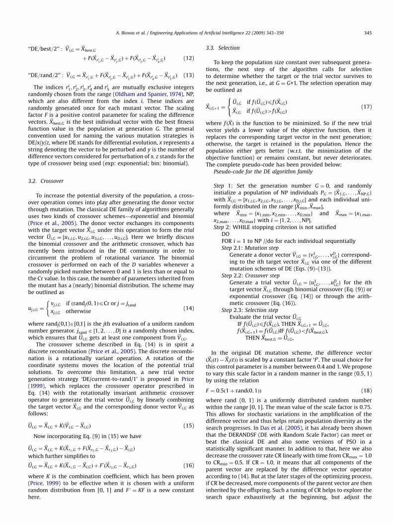
expansion (CFE) scheme was used in this work. Several simulation examples as well as comparisons

of DE with two other state-of-the-art optimization techniques (Particle Swarm Optimization and binary

Genetic Algorithm) over the same problems demonstrate the superiority of the proposed approach

especially for actuating fractional-order plants. The proposed technique may serve as an efficient

alternative for the design of next-generation fractional-order controllers.

& 2008 Elsevier Ltd. All rights reserved.

1. Introduction

Fractional-order dynamic systems and controllers, which arebased on fractional-order calculus (Oldham and Spanier, 1974;Lubich, 1986; Miller and Ross, 1993), have been gaining attentionin several research communities since the last few years(Oustaloup, 1981; Chengbin and Hori, 2004). In Podlubny(1999b), it was advocated that fractional-order calculus wouldplay a major role in a smart mechatronic system. Podlubnyproposed the concept of the fractional-order PIlDm controllers anddemonstrated the effectiveness of such controllers for actuatingthe responses of fractional-order systems in 1999. A few recentworks in this direction as well as schemes for digital andhardware realizations of such systems can be traced in Chenet al. (2004), Nakagawa and Sorimachi (1992) and Chen et al.(2005). Vinagre et al. (2000) proposed a frequency domainapproach based on expected crossover frequency and phasemargin for the same controller design. Petras came up with a

ll rights reserved.

iswas),

ieee.org (A. Abraham),

method based on the pole distribution of the characteristicequation in the complex plane (Petras, 1999). Dorcak et al.(2001) proposed a state-space design approach based on feedbackpole placement. The fractional controller can also be synthesizedby cascading a proper fractional unit to an integer-order controller(Chengbin and Hori, 2004).

Proportional–integral–derivative (PID) controllers have beenused for several decades in industries for process controlapplications. The reason for their wide popularity lies in thesimplicity of design and good performance including lowpercentage overshoot and small settling time for slow processplants (Astrom and Hagglund, 1995). In fractional-order propor-tional–integral–derivative (FOPID) controller, I and D operationsare usually of fractional order; therefore, besides setting theproportional, derivative and integral constants Kp, Td, Ti we havetwo more parameters: the order of fractional integration l andthat of fractional derivative m. Finding an optimal set of values forKp, Ti, Td, l and m to meet the user specifications for a given processplant calls for real parameter optimization in five-dimensionalhyperspace.

Differential evolution (DE) (Price et al., 2005; Storn and Price,1997) has recently become quite popular as a simple and efficientscheme for global optimization over continuous spaces. It hasreportedly outperformed many types of evolutionary algorithms

www.sciencedirect.com/science/journal/eaai

www.elsevier.com/locate/engappai

dx.doi.org/10.1016/j.engappai.2008.06.003

mailto:[email protected]




ARTICLE IN PRESS

A. Biswas et al. / Engineering Applications of Artificial Intelligence 22 (2009) 343–350344

and search heuristics like PSO when tested over both benchmarksand real-world problems (Vesterstrøm and Thomson, 2004). Inthis work, a state-of-the-art version of DE has been used forfinding the optimal values of Kp, Ti, Td, l and m. The design methodfocuses on optimum placing of the dominant closed-loop polesand incorporate the constraints thus obtained using DE algorithm.The optimization-based design process has been tested foractuating the response of four process plants of which two areof integer order and two are of fractional order. The performanceof the DE-based PIlDm controller has been compared with twoother fractional-order controllers designed with the state-of-the-art versions of two recent swarm intelligence-based techniqueswell known as the Hierarchical Particle Swarm Optimizer withTime Varying Acceleration Coefficients (HPSO-TVAC) (Ratnaweeraand Halgamuge, 2004) and the genetic algorithm (Holland, 1975;Cao et al., 2005). Such comparison reflects the superiority of theproposed method in terms of quality of the final solution,convergence speed and robustness.

The rest of the paper is organized as follows. Section 2describes the rudiments of fractional calculus and fractional-ordercontrol systems. Section 3 provides a brief overview of the DEfamily of algorithms and describes a recent state-of-the-artversion of DE called DE/rand/either–or, which was used, in thisspecific task. Section 4 demonstrates how the DE can be applied tothe PIlDm controller design problem when formulated as anoptimization task. Simulation strategies and experimental resultshave been presented and discussed in Section 5 and finally thepaper is concluded with a discussion on future research issues inSection 6.

2. Fractional-order systems: a brief overview

Fractional calculus is a branch of mathematical analysis thatstudies the possibility of taking real number power of thedifferential operator and integration operator. From a purelymathematical point of view, there are several ways to definefractional-order derivatives and integrals. The generalized differ-integrator operator may be put forward as

aDqt f ðtÞ ¼

dqf ðtÞ

½dðt � aÞ�q(1)

where q represents the real order of the differintegral (an n

is used in some literature to denote an integer order), t is theparameter for which the differintegral is taken and a isthe lower limit. Unless otherwise stated, the lower limit willbe 0 and left out of the notation. Caputo used a popular definitionused to compute differintegral in 1960s. The definition forCaputo’s fractional derivative of order l with respect to thevariable t and with the starting point t ¼ 0 goes as follows(Caputo, 1967, 1969):

0Dlt yðtÞ ¼

1

Gð1� dÞ

Z t

0

yðmþ1ÞðtÞdtðt � tÞd

ðg ¼ mþ d; m 2 Z; 0odp1Þ

(2)

where G(Z) is Euler’s gamma function. If go0, then we have afractional integral of order �g given as

0I�gt yðtÞ ¼ 0Dgt yðtÞ ¼

1

Gð�gÞ

Z t

0

yðtÞdtðt � tÞ1þg

ðgo0Þ (3)

One distinct advantage of using Caputo’s definition is that itonly allows for consideration of easily interpretable initialconditions but it is also bounded, which means the derivative ofa constant is equal to zero. In time domain, a fractional-order

system is governed by an n-term inhomogeneous fractional-orderdifferential equation (FDE):

anDbn yðtÞ þ an�1Dbn�1 yðtÞ þ � � � þ a1Db1 yðtÞ þ a0Db0 yðtÞ ¼ uðtÞ (4)

where Dl� 0Dl

t is the Caputo’s fractional derivative of order l.Converting to frequency domain, the fractional-order transferfunction of such a system may be obtained through the Laplacetransform function as follows:

GnðsÞ ¼1

ansbn þ an�1sbn�1 þ � � � þ a1sb1 þ a0sb0(5)

where bk (k ¼ 0, 1, y, n) is an arbitrary real number,bn4bn�14?4b14b040 and ak (k ¼ 0, 1, y, n) is an arbitraryconstant. Finally, we would like to mention here that the Laplacetransform of the fractional derivative might be given asZ 1

0e�stDgyðtÞdt ¼ sgYðsÞ �

Xm

k¼0

sg�k�1yðkÞðyÞ (6)

For go0 (i.e., for the case of a fractional integral) the sum in theright-hand side must be omitted.

3. The DE algorithm and its modification

Like any other evolutionary algorithm, DE starts with apopulation of NP D-dimensional parameter vectors representingthe candidate solutions. We shall denote subsequent generationsin DE by G ¼ 0, 1, y, Gmax. Since the parameter vectors are likelyto be changed over different generations, we may adopt thefollowing notation for representing the ith vector of the popula-tion at the current generation as

~Xi;G ¼ ½x1;i;G; x2;i;G; x3;i;G; . . . ; xD;i;G� (7)

The initial population (at G ¼ 0) should better cover the entiresearch space as much as possible by uniformly randomizingindividuals within the search space constrained by the prescribedminimum and maximum bounds: ~Xmin ¼ fx1;min; x2;min; . . . ; xD;ming

and ~Xmax ¼ fx1;max; x2;max; . . . ; xD;maxg. Hence we may initialize thejth component of the ith vector as

xj;i;0 ¼ xj;min þ randjð0;1Þðxj;max � xj;minÞ (8)

where randj(0,1) is the jth instantiation of a uniformly distributedrandom number lying between 0 and 1. Following steps are takennext: mutation, crossover and selection, which are explainedbelow.

3.1. Mutation

After initialization, DE creates a donor vector ~Vi;G correspond-ing to each population member or target vector ~Xi;G in the currentgeneration through mutation. It is the method of creating thisdonor vector, which differentiates between the various DEschemes. For example, five most frequently referred mutationstrategies implemented in the public-domain DE codes availableonline at http://www.icsi.berkeley.edu/�storn/code.html arelisted below:

‘‘DE=rand=1’’ : ~Vi;G ¼~Xri

1;G þ Fð~Xri

2;G �

~Xri3;GÞ (9)

‘‘DE=best=1’’ : ~Vi;G ¼~Xbest;G þ Fð~Xri

1;G �

~Xri2;GÞ (10)

‘‘DE=target-to-best=1’’ : ~Vi;G ¼~Xi;G

þ Fð~Xbest;G �~Xi;GÞ

þ Fð~Xri1;G �

~Xri2;GÞ (11)

http://www.icsi.berkeley.edu/~storn/code.html

http://www.icsi.berkeley.edu/~storn/code.html

ARTICLE IN PRESS

A. Biswas et al. / Engineering Applications of Artificial Intelligence 22 (2009) 343–350 345

‘‘DE=best=2’’ : ~Vi;G ¼~Xbest;G

þ Fð~Xri1;G �

~Xri2;GÞ þ Fð~Xri

3;G �

~Xri4;GÞ (12)

‘‘DE=rand=2’’ : ~Vi;G ¼~Xri

1;G þ Fð~Xri

2;G �

~Xri3;GÞ þ Fð~Xri

4;G �

~Xri5;GÞ (13)

The indices ri1; r

i2; r

i3; r

i4 and ri

5 are mutually exclusive integersrandomly chosen from the range (Oldham and Spanier, 1974), NP,which are also different from the index i. These indices arerandomly generated once for each mutant vector. The scalingfactor F is a positive control parameter for scaling the differencevectors. ~Xbest;G is the best individual vector with the best fitnessfunction value in the population at generation G. The generalconvention used for naming the various mutation strategies isDE/x/y/z, where DE stands for differential evolution, x represents astring denoting the vector to be perturbed and y is the number ofdifference vectors considered for perturbation of x. z stands for thetype of crossover being used (exp: exponential; bin: binomial).

3.2. Crossover

To increase the potential diversity of the population, a cross-over operation comes into play after generating the donor vectorthrough mutation. The classical DE family of algorithms generallyuses two kinds of crossover schemes—exponential and binomial

(Price et al., 2005). The donor vector exchanges its componentswith the target vector ~Xi;G under this operation to form the trial

vector ~Ui;G ¼ ½u1;i;G;u2;i;G;u3;i;G; . . . ;uD;i;G�. Here we briefly discussthe binomial crossover and the arithmetic crossover, which hasrecently been introduced in the DE community in order tocircumvent the problem of rotational variance. The binomialcrossover is performed on each of the D variables whenever arandomly picked number between 0 and 1 is less than or equal tothe Cr value. In this case, the number of parameters inherited fromthe mutant has a (nearly) binomial distribution. The scheme maybe outlined as

uj;i;G ¼vj;i;G if ðrandjð0;1ÞpCr or j ¼ jrand

xj;i;G otherwise

((14)

where randj(0,1)A[0,1] is the jth evaluation of a uniform randomnumber generator. jrand 2 ½1;2; . . . ;D� is a randomly chosen index,which ensures that ~Ui;G gets at least one component from ~Vi;G.

The crossover scheme described in Eq. (14) is in spirit adiscrete recombination (Price et al., 2005). The discrete recombi-nation is a rotationally variant operation. A rotation of thecoordinate systems moves the location of the potential trialsolutions. To overcome this limitation, a new trial vectorgeneration strategy ‘DE/current-to-rand/1’ is proposed in Price(1999), which replaces the crossover operator prescribed inEq. (14) with the rotationally invariant arithmetic crossoveroperator to generate the trial vector ~Ui;G by linearly combiningthe target vector ~Xi;G and the corresponding donor vector ~Vi;G asfollows:

~Ui;G ¼~Xi;G þ Kð~Vi;G �

~Xi;GÞ (15)

Now incorporating Eq. (9) in (15) we have

~Ui;G ¼~Xi;G þ Kð~Xr1 ;G þ Fð~Xr2 ;G �

~Xr3 ;GÞ �~Xi;GÞ

which further simplifies to

~Ui;G ¼~Xi;G þ Kð~Xr1 ;G �

~Xi;GÞ þ F 0ð~Xr2 ;G �~Xr3 ;GÞ (16)

where K is the combination coefficient, which has been proven(Price, 1999) to be effective when it is chosen with a uniformrandom distribution from [0, 1] and F 0 ¼ KF is a new constanthere.

3.3. Selection

To keep the population size constant over subsequent genera-tions, the next step of the algorithm calls for selection

to determine whether the target or the trial vector survives tothe next generation, i.e., at G ¼ G+1. The selection operation maybe outlined as

~Xi;Gþ1 ¼

~Ui;G if f ð~Ui;GÞpf ð~Xi;GÞ

~Xi;G if f ð~Ui;GÞ4f ð~Xi;GÞ

8<: (17)

where f ð~XÞ is the function to be minimized. So if the new trialvector yields a lower value of the objective function, then itreplaces the corresponding target vector in the next generation;otherwise, the target is retained in the population. Hence thepopulation either gets better (w.r.t. the minimization of theobjective function) or remains constant, but never deteriorates.The complete pseudo-code has been provided below:

Pseudo-code for the DE algorithm family

Step 1: Set the generation number G ¼ 0, and randomlyinitialize a population of NP individuals PG ¼ f

~X1;G; . . . ; ~XNP;Gg

with ~Xi;G ¼ ½x1;i;G; x2;i;G; x3;i;G; . . . ; xD;i;G� and each individual uni-formly distributed in the range ½~Xmin; ~Xmax�,where ~Xmin ¼ fx1;min; x2;min; . . . ; xD;ming and ~Xmax ¼ fx1;max;

x2;max; . . . ; xD;maxg with i ¼ ½1;2; . . . ;NP�.Step 2: WHILE stopping criterion is not satisfied

DOFOR i ¼ 1 to NP //do for each individual sequentiallyStep 2.1: Mutation step

Generate a donor vector ~Vi;G ¼ fv1i;G; . . . ; v

Di;Gg correspond-

ing to the ith target vector ~Xi;G via one of the differentmutation schemes of DE (Eqs. (9)–(13)).

Step 2.2: Crossover step

Generate a trial vector ~Ui;G ¼ fu1i;G; . . . ;u

Di;Gg for the ith

target vector ~Xi;G through binomial crossover (Eq. (9)) orexponential crossover (Eq. (14)) or through the arith-metic crossover (Eq. (16)).

Step 2.3: Selection step

Evaluate the trial vector ~Ui;G

IF f ð~Ui;GÞpf ð~Xi;GÞ, THEN ~Xi;Gþ1 ¼~Ui;G,

f ð~Xi;Gþ1Þ ¼ f ð~Ui;GÞIF f ð~Ui;GÞof ð~Xbest;GÞ,THEN ~Xbest;G ¼

~Ui;G,

In the original DE mutation scheme, the difference vectorð~XiðtÞ � ~XjðtÞÞ is scaled by a constant factor ‘F’. The usual choice forthis control parameter is a number between 0.4 and 1. We proposeto vary this scale factor in a random manner in the range (0.5, 1)by using the relation

F ¼ 0:5ð1þ randð0;1ÞÞ (18)

where rand (0, 1) is a uniformly distributed random numberwithin the range [0, 1]. The mean value of the scale factor is 0.75.This allows for stochastic variations in the amplification of thedifference vector and thus helps retain population diversity as thesearch progresses. In Das et al. (2005), it has already been shownthat the DERANDSF (DE with Random Scale Factor) can meet orbeat the classical DE and also some versions of PSO in astatistically significant manner. In addition to that, here we alsodecrease the crossover rate CR linearly with time from CRmax ¼ 1.0to CRmin ¼ 0.5. If CR ¼ 1.0, it means that all components of theparent vector are replaced by the difference vector operatoraccording to (14). But at the later stages of the optimizing process,if CR be decreased, more components of the parent vector are theninherited by the offspring. Such a tuning of CR helps to explore thesearch space exhaustively at the beginning, but adjust the

ARTICLE IN PRESS


movements of trial solutions finely during the later stages ofsearch, so that they can explore the interior of a relatively smallspace in which the suspected global optimum lies. The timevariation of CR may be expressed in the form of the followingequation:

CR ¼ ðCRmax � CRminÞGmax � G

Gmax

� �þ CRmin (19)

where CRmax and CRmin are the maximum and minimum values ofcrossover rate CR, G is the current generation number and Gmax isthe maximum number of allowable generations. After performinga series of experiments we find that the DE/rand/1/bin scheme(Eq. (9)) equipped with these modifications can outperform allother classical DE variants for the controller design probleminvestigated here. We exclude the detailed comparison results inorder to save space.

�

4. The DE-based design of fractional PIkDl controllers

4.1. The FOPID controller

A PID controller is a generic control loop feedback mechanismwidely used in industrial control systems. The PID controllerattempts to correct the error between a measured process variableand a desired set point by calculating and then outputting acorrective action that can adjust the process accordingly. Aninteger-order PID controller has the following transfer function:

GcðsÞ ¼ Kp þ Kis�1 þ Kds (20)

The PID controller calculation (algorithm) involves threeseparate parameters: the proportional (Kp), the integral (Ki) andderivative (Kd) time constants. The proportional gain determinesthe reaction to the current error, the integral determines thereaction based on the sum of recent errors and the derivativedetermines the reaction to the rate at which the error has beenchanging. The weighted sum of these three actions is used toadjust the process via a control element such as the position of acontrol valve or the power supply of a heating element. The blockdiagram of a generic closed-loop control system involving the PIDcontroller has been shown in Fig. 1.

The real objects or processes that we want to control aregenerally fractional (for example, the voltage–current relation of asemi-infinite lossy RC line). However, for many of them thefractionality is very low. In general, the integer-order approxima-tion of the fractional systems can cause significant differencesbetween mathematical model and real system. The main reasonfor using integer-order models was the absence of solutionmethods for FDEs. PID controllers belong to dominating industrialcontrollers and therefore are objects of steady effort for improve-ments of their quality and robustness. One of the possibilities to

Fig. 1. A generic closed-loop process-control system with PID controller.

improve PID controllers is to use fractional-order controllers withnon-integer derivation and integration parts.

Following the works of Podlubny (1999b), we may go for ageneralization of the PID controller, which can be called the PIlDm

controller because of involving an integrator of order l and adifferentiator of order m. The continuous transfer function of sucha controller has the form

GcðsÞ ¼ Kp þ Tis�l þ Tdsm ðl;m40Þ (21)

The output response of the PIlDm controller in time domain maybe given as

uðtÞ ¼ KpeðtÞ þ KiD�leðtÞ þ KdDmeðtÞ (22)

where l ¼ +1, m ¼ +1 implies normal PID controller, for l ¼ 0,m ¼ +1, we get a normal PD controller, l ¼ +1, m ¼ 0 impliesnormal PI controller and l ¼ 0, m ¼ 0 implies a proportional gain.All these classical types of PID controllers are the special cases ofthe fractional PIlDm controller. As can be perceived from Fig. 2, theFOPID controller generalizes the integer-order PID controller andexpands it from point to plane. This expansion adds moreflexibility to controller design and we can control our real-worldprocesses more accurately.

4.2. Formulation of the objective function

The design approach presented here is based on the root locusmethod (dominant roots method) of synthesizing integral PIDcontrollers (Astrom and Hagglund, 1995). As in the traditional rootlocus method, based on the user specifications of peak overshootMp and rise time trise (or requirements of stability and dampinglevels), we find out the damping ratio x and the un-dampednatural frequency o0 of the closed-loop system to be designed.Then dominant poles will be

p1;2 ¼ �xo0 � jo0

ffiffiffiffiffiffiffiffiffiffiffiffiffiffi1� x2

q¼ �x� jy ðsayÞ (23)

Let the closed-loop transfer function be

CðsÞ

RðsÞ¼

GðsÞ

1þ GðsÞHðsÞ(24)

where the transfer function of the process to be controlled is Gp(s)and that of the controller is Gc(s) ¼ U(s)/E(s) and G(s) ¼ Gc(s)Gp(s).We assume unity feedback gain, i.e., H(s) ¼ 1. From Eq. (24) the

(0, 1)PI

(0, 0)P

(1, 1)PID

(1, 0)PD �

Fig. 2. Generalization of the FOPID controller: from point to plane.

ARTICLE IN PRESS


characteristics equation of the closed-loop system is

1þ GðsÞHðsÞ ¼ 0) 1þ GpðsÞGcðsÞ � 1 ¼ 0 (25)

Now the dominant poles of the system are the zeros of thischaracteristics equation, so they will obviously satisfy theequation. Thus from (25) we get

1þ ½Kp þ Kið�xþ jyÞ�l þ Kdð�xþ jyÞm�Gpð�xþ jyÞ ¼ 0 (26)

This equation has total five unknowns, Kp, Ki, Kd, l and m. Let R

be the real part of the complex expression (26), I the imaginarypart of the complex expression (26) and c the phase an-gle ¼ tan�1(I/R).

Now we define the following objective function:

JðKp;Ki;Kd; l;mÞ ¼ jIj2 þ jRj2 þ c�� 2 (27)

Our goal is to find out an optimal solution set {Kp, Ki, Kd, l, m} forwhich J ¼ 0. Here the above function has been minimized withmodified DE/rand/1/bin algorithm.

4.3. Vector representation in DE

The solution space of Eq. (27) is five-dimensional, the fivedimensions being {Kp, Ki, Kd, l, m}. So each parameter vector in DEhas five components, i.e., the jth population member at Gthgeneration may be given as

~Xj;G ¼ ðKp;Ki;Kd;l;mÞT (28)

From the practical consideration of the PID controller design(Astrom and Hagglund, 1995), we fixed the following numericalranges for each parameter:

1pKpp1000

0pl; dp1

1pTi; Tdp500 (29)

5. Experimental results

5.1. Problem instances

We have tested the proposed method on three specificinstances of the design problem. All the design examples followthe basic framework detailed in Section 4. The first probleminvolves the speed control of a DC motor. First, the uncompen-sated motor can only rotate at 0.1 rad/s with an input voltage of1 V (this was obtained when the open-loop response is simulated).Since the most basic requirement of a motor is that it shouldrotate at the desired speed, the steady-state error of the motorspeed should be less than 1%. The other performance requirementis that the motor must accelerate to its steady-state speed as soon

Table 1Description of the problem instances considered

Problem number Process plant transfer function Gp(s)

I k

ðJsþ bÞðLsþ RÞ þ k2, J ¼ 0.01, b ¼ 0.1, k ¼ 0.01, R ¼ 1, L ¼ 0.5

II s2

50sþ 400III 1

0:8s2:2 þ 0:5s0:9 þ 1IV 1

0:9s0:3 þ 0:6s0:8 þ 1(hypothetical plant)

as it turns on. In this case, we want it to have a settling time of 2 s.Since a speed faster than the reference may damage theequipment, we want to have an overshoot of less than 5%. Thesecond problem also involves a second-order (integer) plant,which is to be controlled for obtaining a peak overshoot MP ¼ 30%and rise time trise ¼ 0.3 s in the closed-loop response.

The third and fourth problem instances involve fractional-order plants. The third one is taken from Podlubny’s seminalpaper on fractional controllers (Podlubny, 1999b). In some cases areal system is better described by such FDEs (Podlubny, 1999a)and from this consideration, it is important to investigate thecontrolling mechanism of such systems through FOPID-typecontrollers. Table 1 summarizes all the test problems along withthe corresponding user specifications.

5.2. Digital realization of the FOPID controller

For a fractional-order differentiator/integrator sr, where r is areal number, its discretization is a key step in digital implementa-tion. Furthermore for control applications, the obtained approx-imate discrete time rational transfer function should be stable andof minimum phase. Continuous fraction expansion (CFE) by Tustinrule enjoys all those desirable properties. By using this method,the discrete transfer function approximating fractional-orderoperators can be expressed as

D�rðzÞ ¼ ðwðz�1ÞÞ

�r¼

2

T

� ��r

CFE1� z�1

1þ z�1

� ��r !

p;q

¼2

T

� ��r Ppðz�1Þ

Qqðz�1Þ(30)

where T is the sampling period and Pp and Qq are polynomials ofdegree p and q, respectively, in the variable z�1. The generalexpression for numerator Pp(z�1) and denominator Qqðz

�1Þ ofD�rðzÞ is given below for p ¼ q ¼ 1,3,5.In this work we have used the Tustin-rule-based CFE where the

sampling time is T ¼ 0.001 s and the order of the approximatemodel is 5 (Table 2).

5.3. Competitor algorithms and parametric set-up

The proposed design method has been extensively comparedwith two state-of-the-art design methods for FOPID controllersbased on the binary GA (Holland, 1975; Cao et al., 2005) and arecently proposed extension of the canonical PSO namely self-organizing HPSO-TVAC (Ratnaweera and Halgamuge, 2004). TheGA-based scheme was proposed by Cao et al. (2005) and uses a50-bit binary string to encode five parameters of the FOPIDcontroller. The fitness functions in Cao’s method employ theintegral of the squared error and absolute error signal value and

Users specification

Maximum overshoot (%) Rise time (s) Steady-state error (%)

5 0.5 4

20 0.1 Not specified

10 0.2 3

5 0.3 3

ARTICLE IN PRESS

Table 2Expressions for numerator and denominator polynomials in the CFE

p ¼ q Pp(Z�1) (k ¼ 1) and Qq(Z�1) (k ¼ 0)

1 ð�1Þkz�1r þ 1

3 ð�1Þkðr3 � 4rÞz�3 þ ð6r2 � 9Þz�2 þ ð�1Þk15z�1r þ 15

5 ð�1Þkðr5 � 20r3 þ 64rÞz�5 þ ð�195r2 þ 15r4 þ 225Þz�4

þ ð�1Þkð105r3 � 735rÞz�3 þ ð420r2 � 1050Þz�2 þ ð�1Þk945z�1r þ 945

Table 3Parameter settings for the different algorithms

HPSO-TVAC Modified DE

Parameter Value Parameter

Pop_size 40 Pop_size

Inertia weight 0.794 CRmax

C1 Linearly varying 0.35-2.4 CRmin

C2 Linearly varying 2.4-0.35 Scale factor F

Vmax 3.00

Re-initialization

velocity

Linearly decaying from Vmax to

0.1Vmax

0 0.5 1 1.5 2 2.5 3 3.50

0.2

0.4

0.6

0.8

1

1.2

1.4

Uncontrolled ResponseFOPID Using MOdified DEInteger PID controllerFOPID Using HPSO-TVACFOPID Using Binary GA

0 2 4 6 8 10 12 14 16 180

0.2

0.4

0.6

0.8

1

1.2

1.4

Uncontrolled ResponseFOPID Using Modified DEInteger PID controllerFOPID Using HPSO-TVACFOPID Using Binary GA

Fig. 3. Unit step response of the closed-loop systems for the test problems: (a) Design Pr

Problem III (fractional-order plant), (d) Design Problem IV (fractional-order plant).


are typically borrowed from the realm of optimal control (Stengel,1994). The HPSO-TVAC algorithm on the other hand uses the sameparticle representation scheme as well as objective function asthat used for the modified DE. Table 3 shows the parametric set-up for these algorithms. We choose the standard set ofparameters, equipped with which the algorithms have beenshown to be at the peak of their performance (over benchmarkfunctions) in the existing literature (Ratnaweera and Halgamuge,2004; Cao et al., 2005; Das et al., 2005). No hand tuning ofparameters has been allowed in any case to make the comparisonfair enough.

Binary GA (Vesterstrøm and Thomson, 2004)

Value Parameter Value

10D Initial Pop_size 50

1.0 No. of bits per gene 50

0.5 Mutation probability 0.01

Uniformly distributed

random number

between 0.5 and 1.0

with mean value 0.75

Uniform crossover

probability

0.6

0 0.2 0.4 0.6 0.8 1 1.20

0.2

0.4

0.6

0.8

1

1.2

1.4

Uncontrolled ResponseFOPID Using Modified DEInteger PID controllerFOPID Using HPSO-TVACFOPID Using Binary GA

0 0.5 1 1.5 2 2.50

0.2

0.4

0.6

0.8

1

1.2

1.4

Uncontrolled ResponseFOPID Using Modified DEInteger PID ControllerFOPID Using HPSO-TVACFOPID Using Binary GA

oblem I (integer-order plant), (b) Design Problem II (integer-order plant), (c) Design

ARTICLE IN PRESS


5.4. Simulation strategy

We run three population-based optimization algorithmsnamely HPSO-TVAC, a modified DE and the binary encoded GAsuggested in Holland (1975) and Cao et al. (2005) over four designproblems according to the user specifications summarized inTable 1. All the algorithms have been developed from scratch in

Table 4The FOPID controller transfer functions as found with modified DE for four test

problems

Process plant transfer function Gp(s) Controller transfer function Gc(s)

k

ðJsþ bÞðLsþ RÞ þ k2, J ¼ 0.01, b ¼ 0.1,

k ¼ 0.01, R ¼ 1, L ¼ 0.5

36:762þ 221:852s�0:668 þ 40:719s0:824

s2

50sþ 400

0:349þ 19:287s�0:949 þ 1:009s0:322

1

0:8s2:2 þ 0:5s0:9 þ 121:22þ 1:37s�0:92 þ 12:05s0:93

1

0:9s0:3 þ 0:6s0:8 þ 1(Hypothetical plant)

1:72þ 41:524s�0:668 þ 1:59s0:824

Table 5Summary of the performance of closed-loop system under different PID controllers aga

Process

plant

Different controllers used Unit step response obtained

Maximum overshoot

(%)7standard

deviation (%)

I Fractional controller using DE 3.117(0.31)

Integer PID controller using DE 4.237(0.34)

Fractional controller using PSO 3.917(0.41)

Fractional controller using GA 6.317(0.87)

II Fractional controller using DE 18.157(0.77)


Fractional controller using PSO 267(0.95)

Fractional controller using GA 327(1.02)

III Fractional controller using DE 7.697(0.23)




IV Fractional controller using DE 1.937(0.089)




0 1 2 3 4 5 6 7 8 9 1010-6

10-4

10-2

100

102

104

No of FEs

Improved DEHPSO-TVACBinary GA

Obj

ectiv

e fu

nctio

n va

lue

(in lo

g sc

ale)

Obj

ectiv

e fu

nctio

n va

lue

(in lo

g sc

ale)

x 104

Fig. 4. Convergence characteristics for an integer and a fra

Visual C++ platform on a Pentium IV, 2.2 GHz PC, with 512 KBcache and 2 GB of main memory in Windows Server 2003environment. The graphs and figures have been obtained usingMATLAB 6.5. Twenty-five independent runs (with different seedsfor the random number generator) were carried out for each of thealgorithms and each run was continued up to 105 functionevaluations (FEs). In case of DE since D ¼ 5, NP ¼ 50 and thisapproximately corresponds to a Gmax ¼ 2000 for 105 FEs. In whatfollows, we report the results for the median run of eachalgorithm (when the runs for a single algorithm have been rankedaccording to their final accuracy).

5.5. Results

Fig. 3 shows the dynamic response characteristics of theclosed-loop systems for design problems I–IV as specified inTable 1. The integer-order PID controller as marked in Fig. 3 wasobtained by minimizing the same objective function (in Eq. (27))in three dimensions, taking l ¼ m ¼ 1. Table 4 provides the FOPIDcontroller transfer functions for four test problems as found with

inst the unit step

Final objective function

values obtainedRise time (s)7standard

deviation (s)

Steady-state error

(%)7standard

deviation (%)

0.3957(0.051) 3.57(0.010) 0.007(0.0000)

0.1017(0.007) 0.17(0.001) 0.007(0.0000)

0.8227(0.091) 1.97(0.021) 0.00017(0.0000)

0.6957(0.088) 2.17(0.056) 0.03127(0.0025)

0.07277(0.001) 07(0.000) 0.007(0.0000)

0.006677(0.001) 0.17(0.001) 0.007(0.0000)

0.1257(0.009) 1.07(0.012) 0.00017(0.0000)

0.1387(0.011) 1.37(0.034) 0.06327(0.0041)

0.0237(0.001) 0.97(0.023) 0.007(0.0000)

0.6517(0.034) 0.47(0.021) 0.007(0.0000)

0.6467(0.056) 1.17(0.071) 0.00017(0.0000)

0.6257(0.077) 1.37(0.081) 0.07117(0.0021)

0.2187(0.015) 1.67(0.034) 0.007(0.0000)

0.4357(0.078) 0.27(0.010) 0.007(0.0000)

0.9827(0.101) 0.17(0.009) 0.00017(0.0000)

1.3127(0.313) 0.37(0.013) 0.05227(0.0037)

Improved DEHPSO-TVACBinary GA

0 1 2 3 4 5 6 7 8 9 10No of FEs

10-6

10-4

10-2

100

102

104

x 104

ctional plant: (a) Integer plant I, (b) Fractional plant I.

ARTICLE IN PRESS


modified DE. Table 5 reports the maximum overshoot (in %), risetime (in s) and steady-state error (in %) for the unit step responseof each closed-loop system under the competitor PID controllersconsidered here. All entries in this table are the mean of the 25independent runs of the modified DE, the HPSO-TVAC and thebinary GA algorithm and come with the respective standarddeviations as well. Convergence characteristics, i.e., how theobjective function value decreases with the number of FEs, areshown in Fig. 4 for one integer-order plant and one fractional-order plant. The graphs indicate that the DE-based method couldfind better solutions consuming lesser amount of computationaltime.

It is noted that for the given common performance criteria onpeak overshoot MP, rise time trise (s), and steady-state error es, thefractional-order controller achieves better results than its integercounterpart in general for the fractional-order plants III and IV.The DE-based FOPID controller provides results closest to thethree user specifications as listed in Table 1 in each case.

6. Discussion and conclusions

An intelligent optimization method for designing FOPIDcontrollers based on the DE is presented in this paper. Fractionalcalculus can provide novel and higher performance extension forFOPID controllers. However, the difficulties of designing FOPIDcontrollers increase, because FOPID controllers also take intoaccount the derivative order and integral order in comparisonwith traditional PID controllers. To design the parameters of theFOPID controllers efficiently, the DE/rand/1/bin algorithm ismodified with respect to its scale factor F and crossover rate CR.The proposed method has been shown to outperform a state-of-the-art version of the PSO algorithm and a binary GA-basedmethod especially for the fractional-order plants. The proposedscheme of fractional PID controller design will thus find extensivecommercial application in the next-generation controller design.

References

Astrom, K., Hagglund, T., 1995. PID Controllers; Theory, Design and Tuning.Instrument Society of America, Research Triangle Park.

Cao, J., Liang, J., Cao, B., 2005. Optimization of fractional order PID controllers basedon genetic algorithms. In: Proceedings of the International Conference onMachine Learning and Cybernetics, Guangzhou, 18–21 August.

Caputo, M., 1967. Linear model of dissipation whose Q is almost frequencyindependent—II. Geophysical Journal of the Royal Astronomical Society 13,529–539.

Caputo, M., 1969. Elasticita e Dissipacione. Zanichelli, Bologna.Chengbin, Ma., Hori, Y., 2004. The application of fractional order PID controller for

robust two-inertia speed control. In: Proceedings of the 4th InternationalPower Electronics and Motion Control Conference, Xi’an, August.

Chen, Y.Q., Xue, D., Dou, H., 2004. Fractional calculus and biomimetic control. In:Proceedings of the First IEEE International Conference on Robotics andBiomimetics (RoBio04), Shengyang, China, August. IEEE.

Chen, Y.Q., Ahn, H., Xue, D., 2005. Robust controllability of interval fractional orderlinear time invariant systems. In: Proceedings of the ASME 2005 InternationalDesign Engineering Technical Conferences & Computers and Information inEngineering Conference, Paper # DETC2005-84744, Long Beach, CA, September24–28, pp. 1–9.

Das, S., Konar, A., Chakraborty, U.K., 2005. Two improved differential evolutionschemes for faster global search. In: ACM-SIGEVO Proceedings of GECCO,Washington, DC, June, pp. 991–998.

Dorcak, L., Petras, I., Kostial, I., Terpak, J., 2001. State-space controller design for thefractional-order regulated system. In: Proceedings of the ICCC’2001, Krynica,pp. 15–20.

Holland, J.H., 1975. Adaptation in Natural and Artificial Systems. University ofMichigan Press, Ann Harbor.

Lubich, C.H., 1986. Discretized fractional calculus. SIAM Journal on MathematicalAnalysis 17 (3), 704–719.

Miller, K.S., Ross, B., 1993. An Introduction to the Fractional Calculus and FractionalDifferential Equations. Wiley, New York.

Nakagawa, M., Sorimachi, K., 1992. Basic characteristics of a fractance device. IEICETransactions on Fundamentals E75-A (12), 1814–1819.

Oldham, K.B., Spanier, J., 1974. The Fractional Calculus. Academic Press, New York.Oustaloup, A., 1981. Fractional order sinusoidal oscillators: optimization and their

use in highly linear FM modulators. IEEE Transactions on Circuits and Systems28 (10), 1007–1009.

Petras, I., 1999. The fractional order controllers: methods for their synthesis andapplication. Journal of Electrical Engineering 50 (9–10), 284–288.

Podlubny, I., 1999a. Fractional Differential Equations. Academic Press, San Diego,Boston, New York, London, Tokyo, Toronto, p. 368.

Podlubny, I., 1999b. Fractional-order systems and PIlDm controllers. IEEE Transac-tions on Automatic Control 44 (1), 208–213.

Price, K., 1999. An introduction to differential evolution. In: Corne, D., Dorigo, M.,Glover, V. (Eds.), New Ideas in Optimization. McGraw-Hill, UK,pp. 79–108.

Price, K., Storn, R., Lampinen, J., 2005. Differential Evolution—A Practical Approachto Global Optimization. Springer, New York.

Ratnaweera, A., Halgamuge, K.S., 2004. Self organizing hierarchical particle swarmoptimizer with time-varying acceleration coefficients. IEEE Transactions onEvolutionary Computation 8 (3), 240–254.

Stengel, R.F., 1994. Optimal Control and Estimation. Dover Publications, New York.Storn, R., Price, K., 1997. Differential evolution—a simple and efficient heuristic for

global optimization over continuous spaces. Journal of Global Optimization 11(4), 341–359.

Vesterstrøm, J., Thomson, R., 2004. A comparative study of differential evolution,particle swarm optimization, and evolutionary algorithms on numericalbenchmark problems. In: Proceedings of the Sixth Congress on EvolutionaryComputation (CEC-2004). IEEE Press, New York, July 6–9.

Vinagre, B.M., Podlubny, I., Dorcak, L., Feliu, V., 2000. On fractional PID controllers:a frequency domain approach. In: Proceedings of IFAC Workshop on DigitalControl-PID’00, Terrassa, Spain.

Documents

Design of fractional-order PIλDμ controllers with an improved differential evolution