Embed Size (px)
Citation preview

Technical University of Munich
Department of Civil, Geo and Environmental Engineering
Chair of Computational Modeling and Simulation
Design Optimization in Early Project Stages A Generative Design Approach to Project Development
Master Thesis
for the Master of Science Program Civil Engineering
Author: Jacqueline Rohrmann
Matriculation number:
Supervisors: Prof. Dr.-Ing. André Borrmann
Simon Vilgertshofer
Date of issue: 15th March 2019
Date of submission: 15th September 2019

Abstract II
Generative design uses the principles of evolution to improve design options iteratively.
It adapts the three operators of selection, crossover, and mutation to generate solu-
tions and evaluate them on design goals.
This study focuses on the potential this method holds for early project stages in the
AEC industry. The goal is to produce a basic model of a project and optimize it in the
aspects relevant to early project development.
To realize this goal, a design concept consisting of variables and constraints has to be
developed. A set of relevant design metrics must be identified to evaluate design op-
tions and determine the direction of the optimization.
This approach is tested on a specific type of Siemens Real Estate office buildings.
Seven variables and eight objectives are identified. A population of 120 solutions is
assessed by the genetic algorithm NSGA-II over 50 generations.
The results include 14 different design options with their parameter values as well as
their individual scoring in each objective. The solutions can easily be compared to each
other based on the provided metrics.
When a well-defined vision of the design and a set of relevant evaluation measures
exist, generative design can provide profitable solutions. It can help optimize a project
and find the right geometry to fulfill non-geometric goals. However, some aspects that
might be trivial to the human designer, but hard to translate into calculatable scores,
will be elaborate to implement.
Keywords: Generative design, optimization, NSGA-II, architecture, project develop-
ment, genetic algorithm, Refinery, multi-objective optimization
Abstract

Zusammenfassung III
Generatives Design ist eine digitale Entwurfsmethodik, die sich die Prinzipien der Evo-
lution zunutze macht. In einem iterativen Prozess werden verschiedene Entwurfsopti-
onen verglichen und verbessert. Dabei werden die drei evolutionären Operatoren Se-
lektion, Rekombination und Mutation angewendet, um neue Lösungsvorschläge zu ge-
nerieren und anschließend auszuwerten.
Diese Studie beschäftigt sich mit dem Potential dieser Methodik für die Projektentwick-
lung in der Bauindustrie. Das Ziel ist es, ein Bauklötzchenmodell eines Projekts zu
erzeugen und dieses im Hinblick auf die relevanten Aspekte der frühen Projektphasen
zu optimieren.
Dafür wird ein abstraktes Design-Konzept benötigt, das die Entwurfsidee mit Hilfe von
Randbedingungen und variablen Eigenschaften beschreibt. Außerdem müssen die
Merkmale festgelegt werden, in denen die Entwurfsoptionen bewertet werden, da
diese die Richtung der Optimierung bestimmen.
Dieser Ansatz wird an einem bestimmten Gebäudetypus von Siemens Real Estate
Bürogebäuden getestet. Dabei werden sieben Entwurfsvariablen und acht Bewer-
tungskategorien festgelegt. Mit dem genetischen Algorithmus NSGA-II wird eine Po-
pulation mit 120 Individuen über 50 Generation optimiert.
Das Ergebnis besteht aus 14 verschiedene Entwurfsoptionen mit den jeweiligen Ei-
genschaften und Merkmalen. Die Ergebnisse lassen sich durch die vorhandene Be-
wertung gut miteinander vergleichen.
Es zeigt sich, dass durch generatives Design nützliche Entwürfe entstehen können,
wenn die Entwurfsvision präzise definiert ist und die Beurteilungsparameter behutsam
gewählt werden. Generatives Design kann dabei helfen, ein Projekt zu optimieren und
die richtige Geometrie im Bezug auf nicht-geometrische Ziele zu finden. Manche As-
pekte, die ein menschlicher Designer automatisch einhält, sind jedoch schwer in mess-
bare Merkmale zu überführen und daher aufwendig in der Implementierung.
Schlüsselwörter: Generative Gestaltung, Optimierung, NSGA-II, Architektur, Projekt-
entwicklung, genetischer Algorithmus, Refinery, Pareto-Optimierung
Zusammenfassung
Table of Content IV
List of Abbreviations and Symbols VI
1 Introduction 7
1.1 Introduction ...................................................................................................7
1.2 Motivation .....................................................................................................9
1.3 Structure ..................................................................................................... 10
2 Generative Design 11
2.1 Background ................................................................................................. 11
2.2 Multi-Objective Optimization ....................................................................... 14
2.3 Genetic Algorithms ...................................................................................... 15
2.4 NSGA-II ...................................................................................................... 18
2.4.1 Fast Nondominated Sorting ........................................................................ 19
2.4.2 Crowding Distance Computation and Operator .......................................... 22
2.4.3 Main loop .................................................................................................... 23
2.4.4 Tournament selection ................................................................................. 24
2.4.5 Crossover and Mutation .............................................................................. 25
2.4.6 Summary .................................................................................................... 28
3 Methodology 29
3.1 Project Development ................................................................................... 29
3.2 Siemens Real Estate Construction Excellence ........................................... 30
3.3 Parametric Model ........................................................................................ 32
3.4 Design Goals .............................................................................................. 39
3.5 Evolution ..................................................................................................... 44
4 Verification 45
4.1 Arithmetic Verification ................................................................................. 45
4.2 Brute Force Verification .............................................................................. 49
5 Implementation 53
5.1 Dynamo ...................................................................................................... 55
5.1.1 Generate ..................................................................................................... 56
Table of Content

Table of Content V
5.1.2 Evaluate ...................................................................................................... 61
5.2 Refinery ...................................................................................................... 64
5.2.1 Punishment Methods .................................................................................. 64
5.2.2 Population Size, Number of Generations and other NSGA-II settings ........ 69
5.2.3 Presentation of Results ............................................................................... 72
6 Experiments 73
6.1 Set-Up ......................................................................................................... 73
6.2 Limitations and Assumptions ...................................................................... 74
6.3 Results ........................................................................................................ 78
6.4 Interview with Siemens ............................................................................... 83
7 Discussion and Outlook 85
References 88
List of Figures 91
List of Tables 96
Appendix A 97
Appendix B 98
List of Abbreviations and Symbols VI
AI Artificial intelligence
ANN Artificial neural networks
BIM Building information modeling
ConEx Siemens Real Estate Construction Excellence
CSV Comma-separated values
EA Evolutionary algorithm
GA Genetic algorithm
GUI Graphical user interface
MOO Multi-objective optimization
NSGA-II Nondominated sorting genetic algorithm
SRE Siemens Real Estate
wp workplace
List of Abbreviations and Symbols

Introduction 7
1.1 Introduction
With the continuous research and public debate on artificial intelligence, it appears
compelling to introduce the computer into the design process as well. Its creativity is
untouched by convention or tradition, so when we give it the freedom to experiment,
unexpected structures might emerge.
As humans, when we are faced with the task to arrange a floorplan, we are immediately
drawn to rectangular shapes. An algorithm, however, has no idea how rooms usually
look like and only respects the constraints we set. So, if the only constraint given is a
list of rooms with desired sizes, it will start experimenting by assembling different
shapes. We can influence the direction of these experiments by setting a goal for the
algorithm, such as minimizing material.
On the right, the layout of an elementary school can
be seen. Joel Simon used this rather traditional floor-
plan and converted it to a room program with size in-
formation for every room as well as adjacency re-
quirements, such as the cafeteria must be placed next
to the kitchen (Simon, 2017). These requirements
were handed to a genetic algorithm (GA) for optimiza-
tion. The goal of the study was set to minimize traffic
flow between classrooms.
1 Introduction
Figure 1 Original floorplan of a school in Maine, USA (Simon, 2017)
Introduction 8
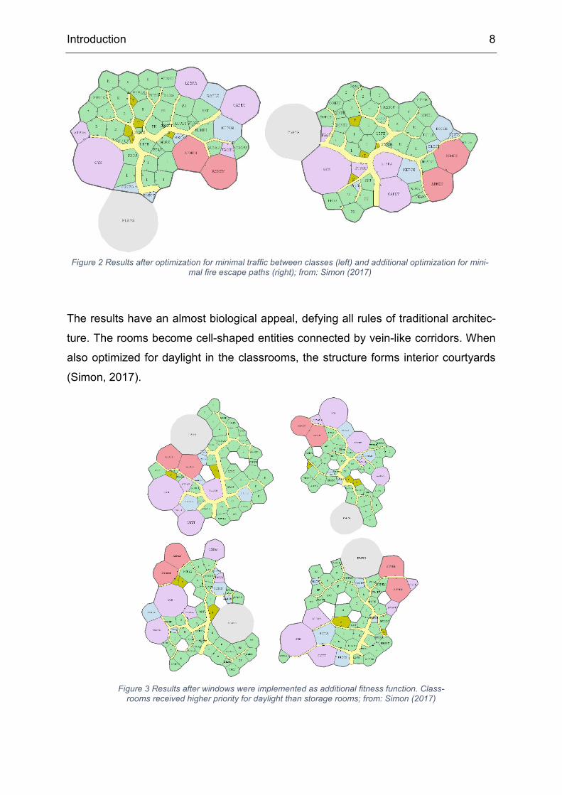
The results have an almost biological appeal, defying all rules of traditional architec-
ture. The rooms become cell-shaped entities connected by vein-like corridors. When
also optimized for daylight in the classrooms, the structure forms interior courtyards
(Simon, 2017).
Figure 2 Results after optimization for minimal traffic between classes (left) and additional optimization for mini-mal fire escape paths (right); from: Simon (2017)
Figure 3 Results after windows were implemented as additional fitness function. Class-rooms received higher priority for daylight than storage rooms; from: Simon (2017)
Introduction 9
Needless to say, these constructs would be expensive in production as well as imprac-
tical in use. However, the experiment can be an inspiration to what effect artificial in-
telligence can have on the design process. At least, it can be a reminder of the bound-
aries we set our creativity as we proceed in age and academic education.
It also highlights the importance of setting clear constraints when working with gener-
ative design. The computer has no inherent understanding of the problem it is faced
with. It can only apply the rules we teach it. Therefore, developing an abstract concept
of the design is the first step in a generative design study. The concept consists of a
set of geometric and arithmetic rules, that limit the space of possibilities just enough
so the results can be useful in the eye of the human designer but leaving enough room
for the algorithm to find unexpectedly positive solutions.
In this study, a respective design concept is developed and optimized in a generative
design workflow. The design problem at hand consists of finding the right position, size,
layout, and desk configuration for a Siemens office building on a pre-defined site. As it
involves meta-elements such as position of the building on-site as well as micro-enti-
ties like a single desk, it is hard for a human designer to regard all aspects simultane-
ously. Experimentation shall determine whether generative design can provide a fruitful
solving mechanism to this problem.
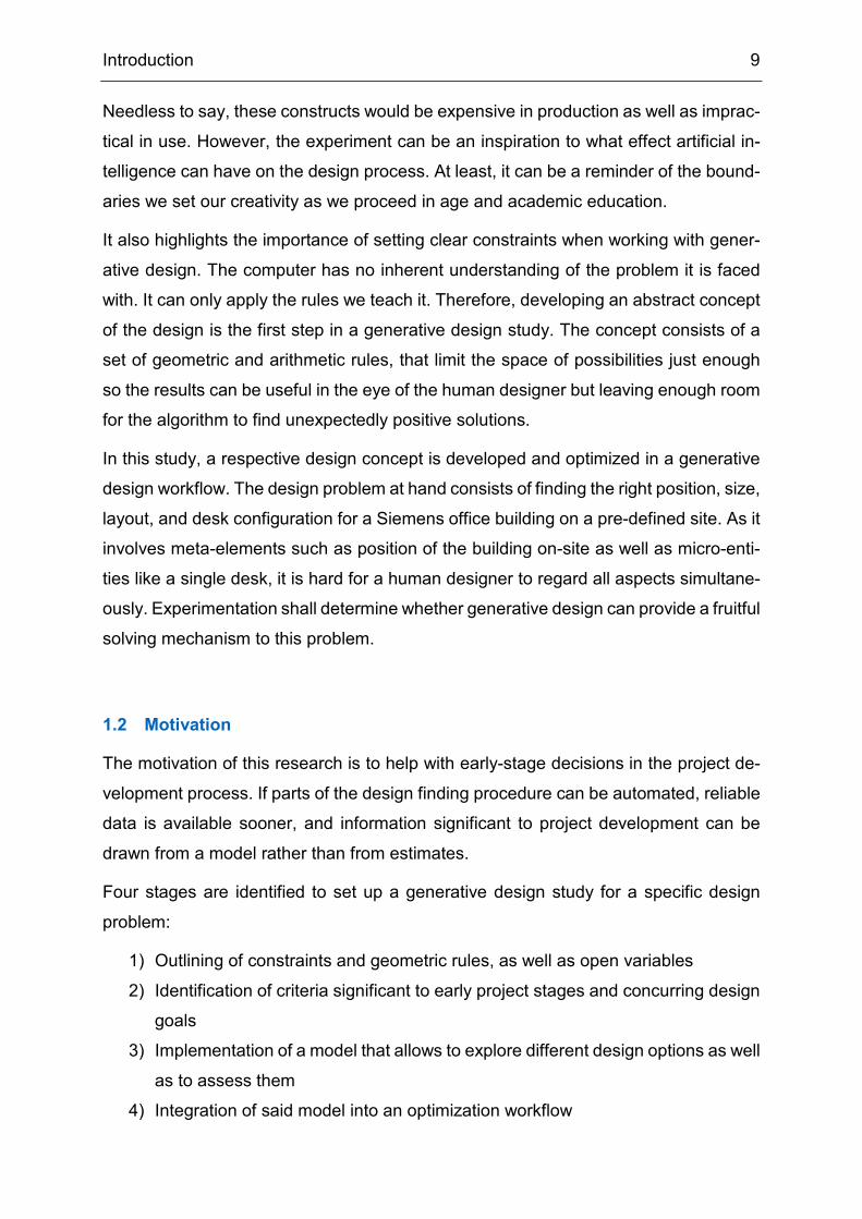
1.2 Motivation
The motivation of this research is to help with early-stage decisions in the project de-
velopment process. If parts of the design finding procedure can be automated, reliable
data is available sooner, and information significant to project development can be
drawn from a model rather than from estimates.
Four stages are identified to set up a generative design study for a specific design
problem:
1) Outlining of constraints and geometric rules, as well as open variables
2) Identification of criteria significant to early project stages and concurring design
goals
3) Implementation of a model that allows to explore different design options as well
as to assess them
4) Integration of said model into an optimization workflow
Introduction 10
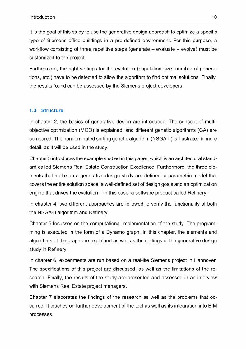
It is the goal of this study to use the generative design approach to optimize a specific
type of Siemens office buildings in a pre-defined environment. For this purpose, a
workflow consisting of three repetitive steps (generate – evaluate – evolve) must be
customized to the project.
Furthermore, the right settings for the evolution (population size, number of genera-
tions, etc.) have to be detected to allow the algorithm to find optimal solutions. Finally,
the results found can be assessed by the Siemens project developers.
1.3 Structure
In chapter 2, the basics of generative design are introduced. The concept of multi-
objective optimization (MOO) is explained, and different genetic algorithms (GA) are
compared. The nondominated sorting genetic algorithm (NSGA-II) is illustrated in more
detail, as it will be used in the study.
Chapter 3 introduces the example studied in this paper, which is an architectural stand-
ard called Siemens Real Estate Construction Excellence. Furthermore, the three ele-
ments that make up a generative design study are defined: a parametric model that
covers the entire solution space, a well-defined set of design goals and an optimization
engine that drives the evolution – in this case, a software product called Refinery.
In chapter 4, two different approaches are followed to verify the functionality of both
the NSGA-II algorithm and Refinery.
Chapter 5 focusses on the computational implementation of the study. The program-
ming is executed in the form of a Dynamo graph. In this chapter, the elements and
algorithms of the graph are explained as well as the settings of the generative design
study in Refinery.
In chapter 6, experiments are run based on a real-life Siemens project in Hannover.
The specifications of this project are discussed, as well as the limitations of the re-
search. Finally, the results of the study are presented and assessed in an interview
with Siemens Real Estate project managers.
Chapter 7 elaborates the findings of the research as well as the problems that oc-
curred. It touches on further development of the tool as well as its integration into BIM
processes.
Generative Design 11
2.1 Background
Design problems are multidimensional by nature (Nagy, 2017a). They consist of a
complex network of non-linear functions, of which the solution is supposed to satisfy a
multitude of goals like function, appearance, economic value, socio-political percep-
tion, etc. Since the time frame of a design process is usually limited, a human designer
cannot possibly explore the entire design space but can only test and improve a minor
amount of designs before deciding on a final solution.
With the advancement of artificial intelligence (AI) arises the idea of a symbiosis be-
tween the human designer and the power of a computer. While the computer has the
computational capacities to produce copious quantities of design solution, the human
designer possesses the intuition and experience to decide what makes a good design.
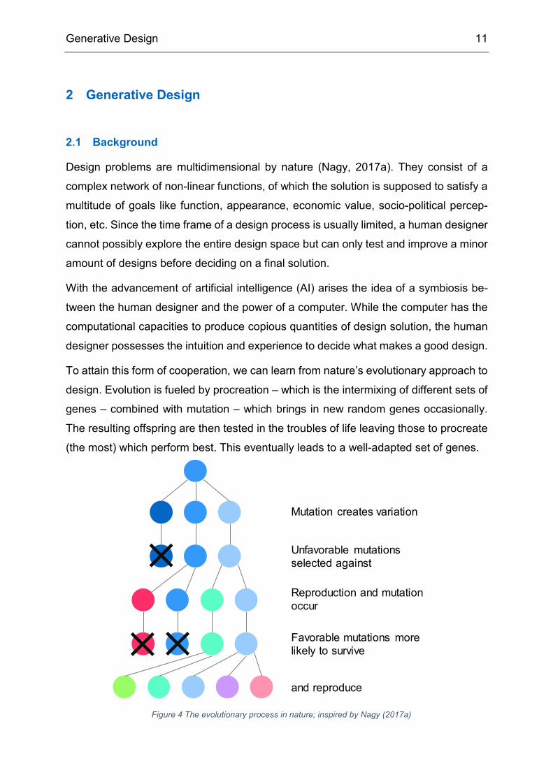
To attain this form of cooperation, we can learn from nature’s evolutionary approach to
design. Evolution is fueled by procreation – which is the intermixing of different sets of
genes – combined with mutation – which brings in new random genes occasionally.
The resulting offspring are then tested in the troubles of life leaving those to procreate
(the most) which perform best. This eventually leads to a well-adapted set of genes.
2 Generative Design
Figure 4 The evolutionary process in nature; inspired by Nagy (2017a)
Mutation creates variation
Unfavorable mutations selected against
Reproduction and mutation occur
Favorable mutations more likely to survive
and reproduce
Generative Design 12
Generative design mimics this process. It is able to “learn from designs it has analyzed,
and apply that knowledge to generate new, better performing designs” (Nagy, 2017b).
Its ability to learn makes this technology part of the larger framework of artificial intelli-
gence. However, it does not make use of artificial neural networks (ANN), but falls into
the category of metaheuristics – or “search algorithms” (Nagy, 2017b). The search
algorithm that is used in most generative design studies is called genetic algorithm
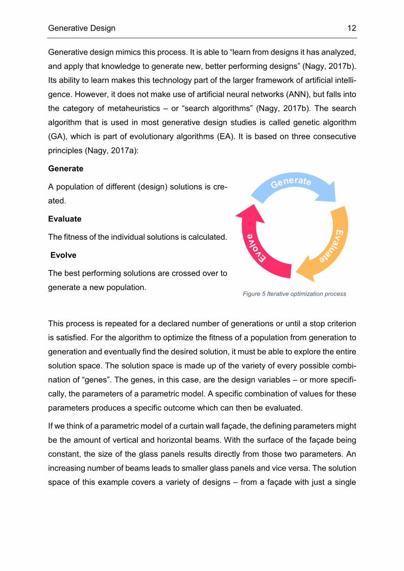
(GA), which is part of evolutionary algorithms (EA). It is based on three consecutive
principles (Nagy, 2017a):
Generate
A population of different (design) solutions is cre-
ated.
Evaluate
The fitness of the individual solutions is calculated.
Evolve
The best performing solutions are crossed over to
generate a new population.
This process is repeated for a declared number of generations or until a stop criterion
is satisfied. For the algorithm to optimize the fitness of a population from generation to
generation and eventually find the desired solution, it must be able to explore the entire
solution space. The solution space is made up of the variety of every possible combi-
nation of “genes”. The genes, in this case, are the design variables – or more specifi-
cally, the parameters of a parametric model. A specific combination of values for these
parameters produces a specific outcome which can then be evaluated.
If we think of a parametric model of a curtain wall façade, the defining parameters might
be the amount of vertical and horizontal beams. With the surface of the façade being
constant, the size of the glass panels results directly from those two parameters. An
increasing number of beams leads to smaller glass panels and vice versa. The solution
space of this example covers a variety of designs – from a façade with just a single
Figure 5 Iterative optimization process
Generative Design 13
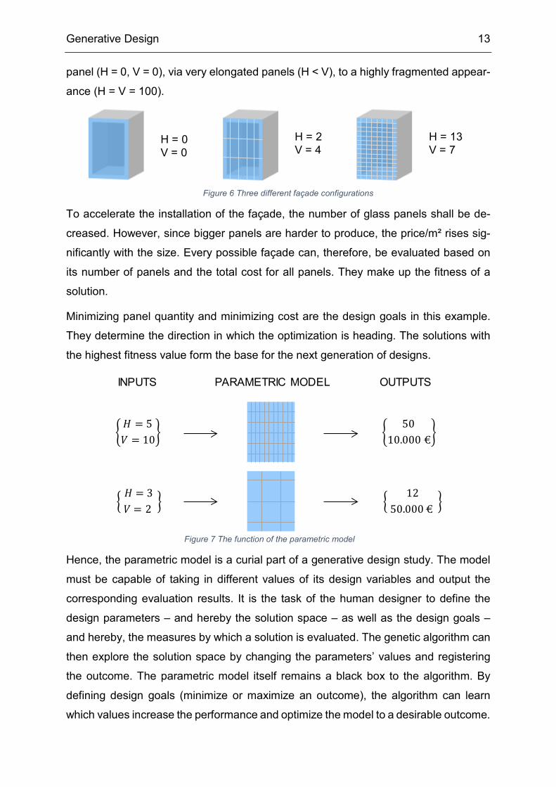
panel (H = 0, V = 0), via very elongated panels (H < V), to a highly fragmented appear-
ance (H = V = 100).
To accelerate the installation of the façade, the number of glass panels shall be de-
creased. However, since bigger panels are harder to produce, the price/m² rises sig-
nificantly with the size. Every possible façade can, therefore, be evaluated based on
its number of panels and the total cost for all panels. They make up the fitness of a
solution.
Minimizing panel quantity and minimizing cost are the design goals in this example.
They determine the direction in which the optimization is heading. The solutions with
the highest fitness value form the base for the next generation of designs.
Hence, the parametric model is a curial part of a generative design study. The model
must be capable of taking in different values of its design variables and output the
corresponding evaluation results. It is the task of the human designer to define the
design parameters – and hereby the solution space – as well as the design goals –
and hereby, the measures by which a solution is evaluated. The genetic algorithm can
then explore the solution space by changing the parameters’ values and registering
the outcome. The parametric model itself remains a black box to the algorithm. By
defining design goals (minimize or maximize an outcome), the algorithm can learn
which values increase the performance and optimize the model to a desirable outcome.
Figure 6 Three different façade configurations
Figure 7 The function of the parametric model
H = 0V = 0
H = 2V = 4
H = 13V = 7
INPUTS PARAMETRIC MODEL OUTPUTS
𝐻 = 5𝑉𝑉 = 10
𝐻 = 3 𝑉𝑉 = 2
5010.000 €
12
50.000 €
Generative Design 14
2.2 Multi-Objective Optimization
The complexity of the design process usually arises from the multitude of criteria that
are to be satisfied but contradict each other in nature. For example, maximizing the
comfort of an apartment leads to an increased floor area, but at the same time, mini-
mizing rent leads to a decreasing floor area.
Finding optimal decisions in the presence of two or more conflicting goals is called
multi-objective optimization (MOO). “For a nontrivial multi-objective optimization prob-
lem, no single solution exists that simultaneously optimizes each objective” (Multi-
objective optimization, 2019). A trade-off situation occurs, in which no objective func-
tion can be increased in value without reducing at least one of the other objective val-
ues. Hence, there cannot be one single solution to satisfy all objectives, but instead,
several Pareto optimal solutions exist. A solution is called Pareto optimal or nondomi-
nated when none of its objective values can be improved without decreasing some of
its other values. Therefore, no solution exists that performs better in all of the objec-
tives.
From a mathematical perspective, a MOO-problem can be described as:
min�𝑓𝑓1(𝑥𝑥),𝑓𝑓2(𝑥𝑥), … ,𝑓𝑓𝑘𝑘(𝑥𝑥)�;
𝑠𝑠, 𝑡𝑡, 𝑥𝑥 ∈ 𝑋𝑋;
(Miettinen, 1999)
The functions 𝑓𝑓1 to 𝑓𝑓𝑘𝑘 represent objective functions, with 𝑘𝑘 being the number of objec-
tives. A vector of input data 𝑋𝑋 describes every possible design in the system. 𝑋𝑋 is
usually limited by some constraint functions. Maximizing a particular objective function
can be achieved by minimizing its negative. “An element 𝑥𝑥∗ ∈ X is called a feasible
solution or a feasible decision. A vector 𝑧𝑧∗ ∶= 𝑓𝑓(𝑥𝑥∗) ∈ 𝑅𝑅𝑘𝑘 for a feasible solution 𝑥𝑥∗ is
called an objective vector or an outcome “ (Multi-objective optimization, 2019).
Generative Design 15
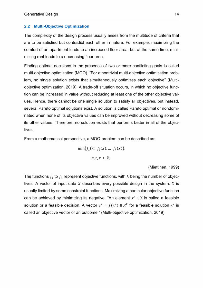
The goal of a MOO is to find a set of nondominated solutions. A solution 𝑥𝑥1 ∈ X domi-
nates another solution, if
1. 𝑓𝑓𝑖𝑖(𝑥𝑥1) ≤ 𝑓𝑓𝑖𝑖(𝑥𝑥2) 𝑓𝑓𝑓𝑓𝑓𝑓 𝑎𝑎𝑎𝑎𝑎𝑎 𝑖𝑖𝑖𝑖𝑖𝑖𝑖𝑖𝑖𝑖𝑖𝑖𝑠𝑠 𝑖𝑖 ∈ {1, 2, … ,𝑘𝑘} and
2. 𝑓𝑓𝑗𝑗(𝑥𝑥1) < 𝑓𝑓𝑗𝑗(𝑥𝑥2) 𝑓𝑓𝑓𝑓𝑓𝑓 𝑎𝑎𝑡𝑡 𝑎𝑎𝑖𝑖𝑎𝑎𝑠𝑠𝑡𝑡 𝑓𝑓𝑖𝑖 𝑖𝑖𝑖𝑖𝑖𝑖𝑖𝑖𝑥𝑥 𝑗𝑗 ∈ {1, 2, … , 𝑘𝑘}. (Miettinen, 1999)
All solutions not dominated by any other solution form the Pareto frontier. It is the goal
of generative design to deliver a diverse set of solutions converging near the Pareto
frontier. This enables a human decision-maker to pick a favorable design solution
knowing that it cannot be optimized further.
2.3 Genetic Algorithms
Genetic algorithms (GA) are used for solving multi-objective optimization (MOO) prob-
lems. The first-ever GA was proposed by John Holland in his book “Adaptation in Nat-
ural and Artificial Systems” (1975).
“It is possible to give genetic processes an algorithmic formulation that
makes them available as control procedures in a wide variety of situa-
tions. By using an appropriate production (rule-based) language, it is even
possible to construct sophisticated models of cognition wherein the ge-
netic algorithm, applied to the productions, provides the system with the
means of learning from experience.”
John Holland (Holland, 1984).
Figure 8 “Point C is not on the Pareto frontier because it is dominated by both point A and point B. Points A and B are not strictly dominated by any other, and hence lie on the frontier” (Dréo, 2006); inspired by Dréo (2006)
A
B
C
f1(A) > f2(A)
f1(B) < f2(B)
Pareto front
f1
f2
Generative Design 16
Holland translated the principles of evolution into a computational algorithm. His model
proved to “search the space of chromosomes in a way much more subtle than a ‘ran-
dom search with preservation of the best ‘” (Holland, 1984).
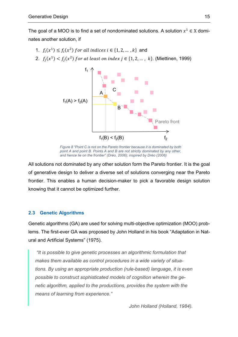
In general, the workflow of a GA can be described as follows:
An initial population of individuals is created randomly. They form the parent population
of the first generation. Then the fitness of each individual is calculated. If the fitness
value of one of the solutions satisfies a stop criterion, the algorithm ends. If not, the
evolutionary principles of selection, breeding, and mutation are applied. Two individu-
als of the first generation are selected to mate, meaning their chromosomes get
crossed over to form a new individual – the children population of the first generation.
Then mutation is randomly applied to the children to bring in random fresh, possibly
fitter DNA.
Afterward, the fitness of the individuals in the children population is calculated. To-
gether with the parent population, all individuals of the first generation get sorted by
their achieved fitness level. The process of ranking the children population together
with the parent population is called elitism. It ensures the preservation of previously
found good solutions. The highest-ranking individuals form the next generation in the
optimization process.
Figure 9 Basic model of a genetic algorithm (GA); inspired by Nagy, 2017b
Generate initial population
Calculate fitness of individuals
Roulette selection of parents
Crossover to produce children
Mutation of children
Calculate fitness of children
New generation by “Elitism”
Satisfy stop
criterion
Start
End
Generative Design 17
Since the early model developed by Holland, different variations of the genetic algo-
rithms (GA) or evolutionary algorithms (EA) have been proposed. They vary mostly in
the way they rank and select solutions for the new parent population.
Early GAs with low computational complexity but no elitism are (Samuelson Hong,
2012):
• VEGA (Vector evaluated GA) (Schaffer, 1985)
• MOGA (Multi-objective GA) (Fonseca & Fleming, 1993)
• NPGA (Niched Pareto GA) (Horn, Nafpliotis & Goldberg, 1994)
They either fail to provide a diverse set of solution or converge to the Pareto frontier
very slowly. Elitism, however, has shown to speed up the performance of a GA while
preserving good solutions once they are found (Deb, Pratap, Agarwal, & Meyarivan,
2002). In the following three commonly known elitist GAs are discussed (Samuelson
Hong, 2012).
PAES – Pareto Archived Evolution Strategy (Knowles & Corne, 1999)
The PAES is the simplest of the three. It keeps a population size of 1 and uses local
search to optimize the solution. Previously found solutions are stored in a reference
archive against which candidate solutions are compared by Pareto dominance
(Knowles & Corne, 1999).
While it ensures the preservation of previously found solutions, the lack of population
size slows down the system, and the overall performance is based on the size of the
searched neighborhood (Samuelson Hong, 2012).
SPEA – Strength Pareto Evolutionary Algorithm (Zitzler & Thiele, 1999)
SPEA uses an external archive as well as a population size that is usually bigger than
the size of the archive (Brownlee, 2015). It ranks solutions based on a combination of
domination and estimation of density of the Pareto front. However, these calculations
are computationally expensive (Samuelson Hong, 2012).
NSGA – Nondominated Sorting GA (Srinivas & Deb, 1994)
NSGA uses fast nondominated sorting to compute the domination rank of a solution
and crowding-distance computation to achieve a diverse set of solutions. Initially, the
algorithm lacked elitism and had a computational complexity of O(MN³) for M objec-
Generative Design 18
tives and N population size, making the algorithm cubically more expensive with in-
creasing population size. However, a new version of the algorithm was introduced in
2000 called NSGA-II. It has a computational complexity of O(MN²) and is elitist as the
parents and the offspring are combined before ranking. NSGA-II gained much appre-
ciation and is widely used in optimization problems (Samuelson Hong, 2012) (Garcia
& Trinh, 2019) (Machairas, Tsangarassoulis, & Kleo, 2014).
Different MOO problems require different solution strategies. In the design problem at
hand, it is very important to provide a diverse set of solutions, so that a human decision-
maker can choose a design favorite based on his or her subjective preferences.
NSGA-II has proven to outperform PAES and SPEA in its ability to find a diverse set
of solutions (Deb, Pratap, Agarwal, & Meyarivan, 2002). This is also the case when
compared to the improved version SPEA2 (Zitzler, Laumanns, & Thiele, 2001). SPEA2
shows less clustering, but NSGA-II provides a broader spread of solutions, i.e., “found
solutions closer to the outlying edges of the Pareto-optimal front” (Kunkle, 2005).
Therefore, it is chosen for the study at hand and explained in more detail in the follow-
ing chapter.
2.4 NSGA-II
Any algorithm striving to solve a MOO problem can be rated by its capability to accom-
plish the following goals (Chiandussi, Codegone, Ferrero, & Varesio, 2012):
• its preservation of previously found nondominated points
• its progress toward the Pareto front (convergence rate)
• the diversity of points on the Pareto front it provides
• its ability to provide the human decision-maker with an appropriately sized num-
ber of solution points for selection
NSGA-II uses three characteristic properties to enhance its optimization – a fast non-
dominated sorting approach, a fast crowded distance estimation procedure, and a sim-
ple crowded-comparison operator (Yusoff, Ngadiman, & Zain, 2011). The algorithm
sorts a population into hierarchic sub-populations based on their rank of Pareto domi-
nance. Within a group, the similarity of solutions is measured to maintain diversity. Deb
et al. (2002) state that in several different test problems “NSGA-II was able to maintain
Generative Design 19
a better spread of solutions and converge better in the obtained nondominated front
comparted to […] PAES and SPEA” (Deb et al., 2002).
A closer look into the elements that make up NSGA-II is given in the following chapter
concluded by an overview of the entire workflow.
2.4.1 Fast Nondominated Sorting
A crucial question concerning MOO problems is: In the face of multiple objectives, how
do you compare one solution to another? How can the overall fitness of a solution be
calculated so that the solutions of a population can be ranked amongst each other?
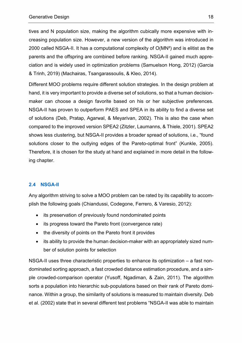
The NSGA-II uses a fast procedure of sorting solutions into groups. Every solution p
receives a domination count np “the number of solutions which dominate the solution
p” and Sp “a set of solutions that the solution p dominates” (Deb et al., 2002). This
involves O(MN²) comparisons (Deb et al., 2002).
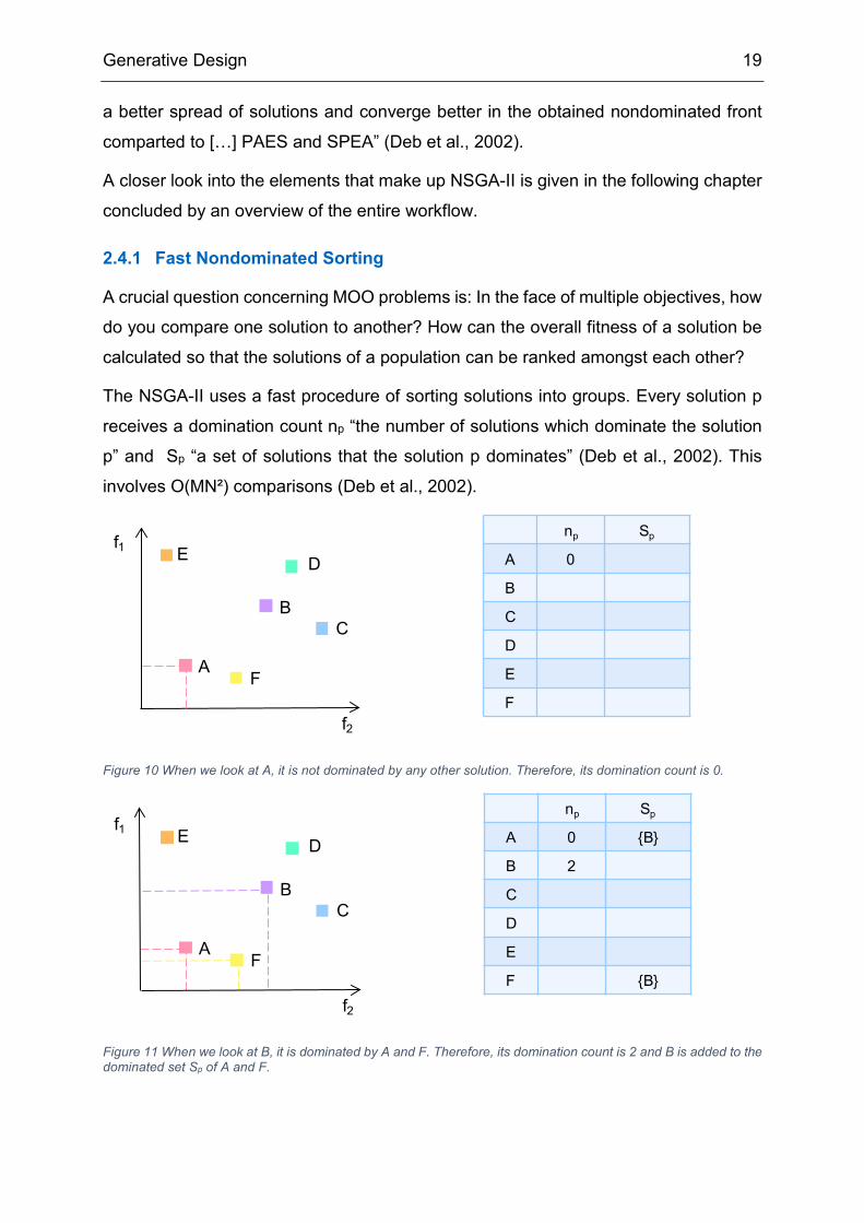
Figure 10 When we look at A, it is not dominated by any other solution. Therefore, its domination count is 0.
Figure 11 When we look at B, it is dominated by A and F. Therefore, its domination count is 2 and B is added to the dominated set Sp of A and F.
A
BC
f1
f2
E
F
D
np Sp
A 0
B
C
D
E
F
A
BC
f1
f2
E
F
D
np Sp
A 0 {B}
B 2
C
D
E
F {B}
Generative Design 20
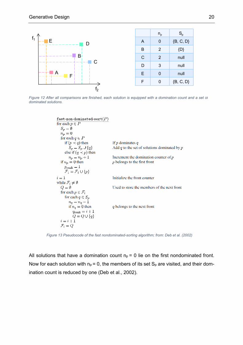
All solutions that have a domination count np = 0 lie on the first nondominated front. Now for each solution with np = 0, the members of its set Sp are visited, and their dom-
ination count is reduced by one (Deb et al., 2002).
A
BC
f1
f2
E
F
D
np Sp
A 0 {B, C, D}
B 2 {D}
C 2 null
D 3 null
E 0 null
F 0 {B, C, D}
Figure 12 After all comparisons are finished, each solution is equipped with a domination count and a set of dominated solutions.
Figure 13 Pseudocode of the fast nondominated-sorting algorithm; from: Deb et al. (2002)

Generative Design 21
Afterward, all solutions with np = 0 are grouped as the second nondominated front. Now
the members in the sets of these solutions are visited. This process is continued until
all solutions are grouped into fronts (Deb et al., 2002).
Figure 14 In the first step, all solutions with a domination count of 0 are grouped into the first front. The members of their dominated sets Sp receive a reduction of 1 in their domination count
Figure 15 In the second step, this process repeated with the solutions that now have a domination count of 0.
Figure 16 This process is repeated until all solutions are sorted into fronts.
np Sp
A 0 {B, C, D}
B 2 {D}
C 2 null
D 3 null
E 0 null
F 0 {B, C, D}
np Sp
A - -
B 0 {D}
C 0 null
D 1 null
E - -
F - -
np Sp
A - -
B - -
C - -
D 0 null
E - -
F - -
np Sp
A - -
B 0 {D}
C 0 null
D 1 null
E - -
F - -
A
BC
f1
f2
E
F
D
1st front
2nd front
3rd front
Generative Design 22
2.4.2 Crowding Distance Computation and Operator
As earlier mentioned, it is desired that, along with convergence to the Pareto optimal
front, the algorithm also maintains a level of variety in its solutions. This helps to avoid
convergence to local minima and offers a diverse set of options to the human decision-
maker. This means – when at the same fitness level – a solution from a less crowded
region is preferred to a solution in a crammed region. To estimate the density of a
solution’s neighborhood, the NSGA-II established the crowding distance computation.
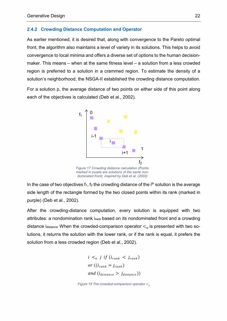
For a solution p, the average distance of two points on either side of this point along
each of the objectives is calculated (Deb et al., 2002).
In the case of two objectives f1, f2 the crowding distance of the ith solution is the average
side length of the rectangle formed by the two closed points within its rank (marked in
purple) (Deb et al., 2002).
After the crowding-distance computation, every solution is equipped with two
attributes: a nondomination rank irank based on its nondominated front and a crowding
distance idistance. When the crowded-comparison operator <𝑛𝑛 is presented with two so-
lutions, it returns the solution with the lower rank, or if the rank is equal, it prefers the
solution from a less crowded region (Deb et al., 2002).
Figure 17 Crowding distance calculation (Points marked in purple are solutions of the same non-dominated front); inspired by Deb et al. (2002)
𝑖𝑖 <𝑖𝑖 𝑗𝑗 𝑖𝑖𝑓𝑓 (𝑖𝑖𝑓𝑓𝑎𝑎𝑖𝑖𝑘𝑘 < 𝑗𝑗𝑓𝑓𝑎𝑎𝑖𝑖𝑘𝑘)
𝑓𝑓𝑓𝑓 ((𝑖𝑖𝑓𝑓𝑎𝑎𝑖𝑖𝑘𝑘 = 𝑗𝑗𝑓𝑓𝑎𝑎𝑖𝑖𝑘𝑘)
𝑎𝑎𝑖𝑖𝑖𝑖 (𝑖𝑖𝑖𝑖𝑖𝑖𝑠𝑠𝑡𝑡𝑎𝑎𝑖𝑖𝑖𝑖𝑖𝑖 > 𝑗𝑗𝑖𝑖𝑖𝑖𝑠𝑠𝑡𝑡𝑎𝑎𝑖𝑖𝑖𝑖𝑖𝑖))
Figure 18 The crowded-comparison operator <𝑖𝑖
i-1
f1
f2
i
0
1i+1
Generative Design 23
2.4.3 Main loop
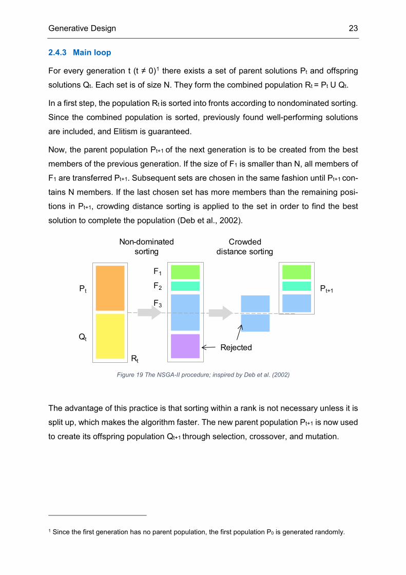
For every generation t (t ≠ 0)1 there exists a set of parent solutions Pt and offspring
solutions Qt. Each set is of size N. They form the combined population Rt = Pt U Qt.
In a first step, the population Rt is sorted into fronts according to nondominated sorting.
Since the combined population is sorted, previously found well-performing solutions
are included, and Elitism is guaranteed.
Now, the parent population Pt+1 of the next generation is to be created from the best
members of the previous generation. If the size of F1 is smaller than N, all members of
F1 are transferred Pt+1. Subsequent sets are chosen in the same fashion until Pt+1 con-
tains N members. If the last chosen set has more members than the remaining posi-
tions in Pt+1, crowding distance sorting is applied to the set in order to find the best
solution to complete the population (Deb et al., 2002).
The advantage of this practice is that sorting within a rank is not necessary unless it is
split up, which makes the algorithm faster. The new parent population Pt+1 is now used
to create its offspring population Qt+1 through selection, crossover, and mutation.
1 Since the first generation has no parent population, the first population P0 is generated randomly.
Non-dominated sorting
Crowded distance sorting
Pt
Qt
Rt
F1
F2
F3
Pt+1
Rejected
Figure 19 The NSGA-II procedure; inspired by Deb et al. (2002)

Generative Design 24
2.4.4 Tournament selection
In the selection process members of a parent population are chosen to be inserted into
a mating pool. The solutions in the mating pool are used to generate offspring. Better
solutions are to procreate more than lower-performing solutions in hopes of creating
offspring with higher fitness. The selection pressure describes the “degree to which the
better individuals are favored” (Sivanandam & Deepa, 2008). The selection pressure
pushes the GA to improve the population fitness. Therefore, a higher selection pres-
sure accelerates the convergence rate to the Pareto front. However, when the selec-
tion pressure is too high, the GA might prematurely converge to a local minimum.
To select solutions for mating, tournaments are held among the members of a parent
population. How these tournaments are executed, determines the selection pressure.
The procedure used in NSGA-II is called binary tournament selection. Two individuals
are randomly chosen and compete against each other. The winner gets determined
through the crowding distance operator, which means the solution with the lower dom-
ination rank irank wins unless the competitors have the same rank in which case the
solution with lower crowding distance idistance wins (Deb et al., 2002).
A copy of the winner enters the mating pool. The original solution is still available for
tournament, which means better solutions have a higher chance of entering the mating
pool several times. Consequently, it will produce more offspring (Sivanandam &
Deepa, 2008). The tournaments get repeated until the mating pool is filled. For in-
stance, a binary tournament for a population of 6 solutions {A, B, C, D, E, F} (in order
of fitness) could look like this:
Generative Design 25
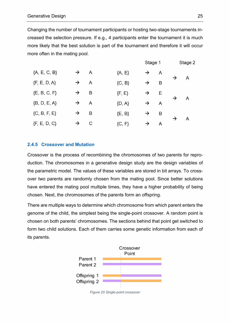
Changing the number of tournament participants or hosting two-stage tournaments in-
creased the selection pressure. If e.g., 4 participants enter the tournament it is much
more likely that the best solution is part of the tournament and therefore it will occur
more often in the mating pool.
2.4.5 Crossover and Mutation
Crossover is the process of recombining the chromosomes of two parents for repro-
duction. The chromosomes in a generative design study are the design variables of
the parametric model. The values of these variables are stored in bit arrays. To cross-
over two parents are randomly chosen from the mating pool. Since better solutions
have entered the mating pool multiple times, they have a higher probability of being
chosen. Next, the chromosomes of the parents form an offspring.
There are multiple ways to determine which chromosome from which parent enters the
genome of the child, the simplest being the single-point crossover. A random point is
chosen on both parents’ chromosomes. The sections behind that point get switched to
form two child solutions. Each of them carries some genetic information from each of
its parents.
Figure 20 Single-point crossover
Parent 1Parent 2
Offspring 1Offspring 2
Crossover Point
Generative Design 26
This form of crossover can be performed with more than one point, in which case it is
called two-point or multi-point crossover (Sivanandam & Deepa, 2008).
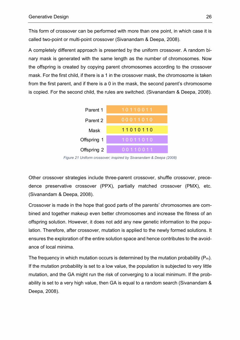
A completely different approach is presented by the uniform crossover. A random bi-
nary mask is generated with the same length as the number of chromosomes. Now
the offspring is created by copying parent chromosomes according to the crossover
mask. For the first child, if there is a 1 in the crossover mask, the chromosome is taken
from the first parent, and if there is a 0 in the mask, the second parent’s chromosome
is copied. For the second child, the rules are switched. (Sivanandam & Deepa, 2008).
Other crossover strategies include three-parent crossover, shuffle crossover, prece-
dence preservative crossover (PPX), partially matched crossover (PMX), etc.
(Sivanandam & Deepa, 2008).
Crossover is made in the hope that good parts of the parents’ chromosomes are com-
bined and together makeup even better chromosomes and increase the fitness of an
offspring solution. However, it does not add any new genetic information to the popu-
lation. Therefore, after crossover, mutation is applied to the newly formed solutions. It
ensures the exploration of the entire solution space and hence contributes to the avoid-
ance of local minima.
The frequency in which mutation occurs is determined by the mutation probability (Pm).
If the mutation probability is set to a low value, the population is subjected to very little
mutation, and the GA might run the risk of converging to a local minimum. If the prob-
ability is set to a very high value, then GA is equal to a random search (Sivanandam &
Deepa, 2008).
Figure 21 Uniform crossover; inspired by Sivanandam & Deepa (2008)
1 0 1 1 0 0 1 1Parent 1
Parent 2
Offspring 1
Offspring 2
0 0 0 1 1 0 1 0
1 1 0 1 0 1 1 0
1 0 0 1 1 0 1 0
0 0 1 1 0 0 1 1
Mask
Generative Design 27
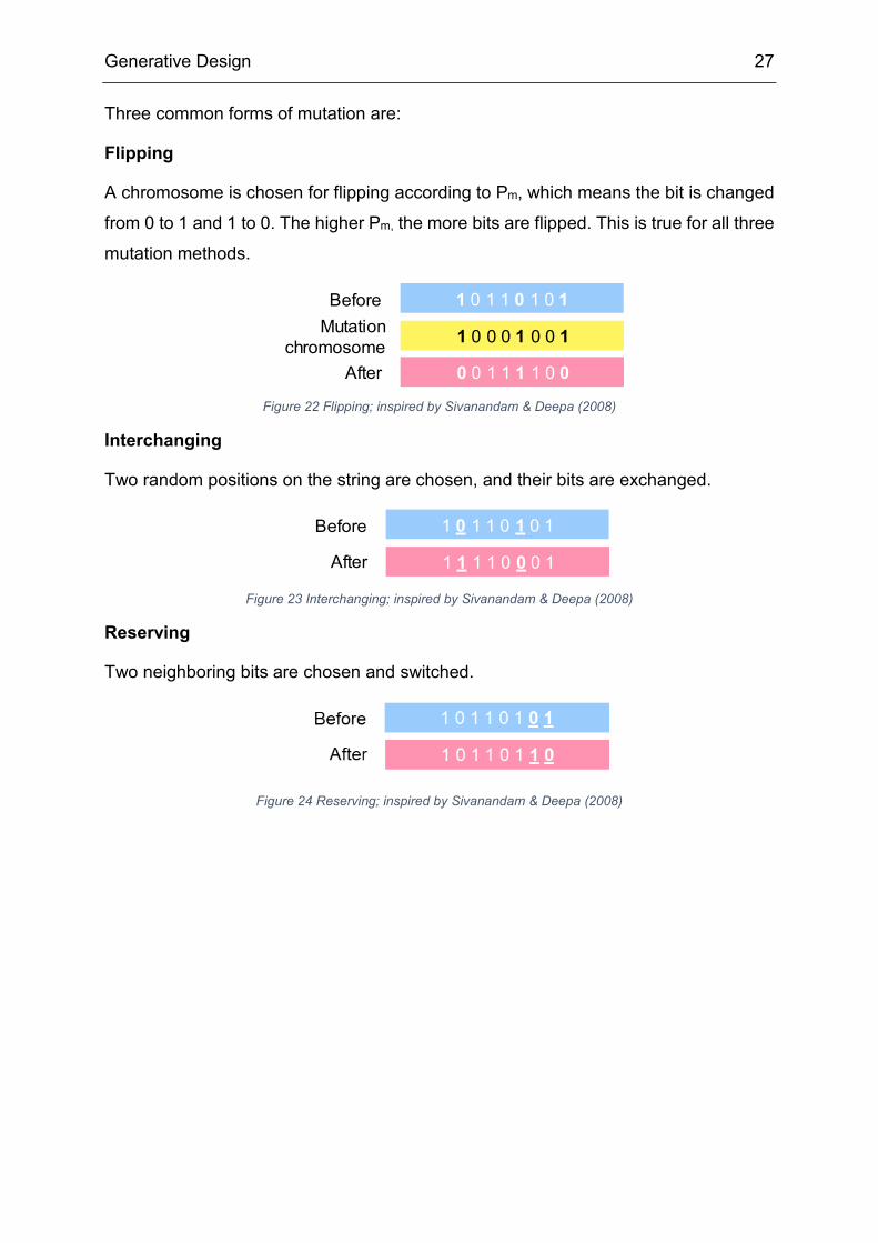
Three common forms of mutation are:
Flipping
A chromosome is chosen for flipping according to Pm, which means the bit is changed
from 0 to 1 and 1 to 0. The higher Pm, the more bits are flipped. This is true for all three
mutation methods.
Interchanging
Two random positions on the string are chosen, and their bits are exchanged.
Reserving
Two neighboring bits are chosen and switched.
Before
After
1 0 1 1 0 1 0 1
1 0 0 0 1 0 0 1
0 0 1 1 1 1 0 0
Mutation chromosome
Before
After
1 0 1 1 0 1 0 1
1 1 1 1 0 0 0 1
Figure 22 Flipping; inspired by Sivanandam & Deepa (2008)
Figure 23 Interchanging; inspired by Sivanandam & Deepa (2008)
Figure 24 Reserving; inspired by Sivanandam & Deepa (2008)

Generative Design 28
2.4.6 Summary
Gen
erat
ion
Rt
cons
istin
g of
pa
rent
pop
ulat
ion
Pta
nd o
ffspr
ing
popu
latio
n Q
t
Pt
Qt
Rt
F 3i-1
i
i+1
f 1
f 2
Indi
vidu
als
F 1F 2F 4
F 4F 1 F 2 F 3
Rt+
1 Pt+
1
13
56
15
Pt+
1
Qt+
1
Rt+
1
Indi
vidu
als
of b
oth
popu
latio
ns a
re
sorte
d in
to fr
onts
ac
cord
ing
to n
on-
dom
inat
ed s
ortin
g
Par
ent p
opul
atio
n of
the
next
ge
nera
tion
is fi
lled
up w
ith fr
onts
.In
cas
e of
a fr
ont
need
ed to
be
split
, cr
owde
d di
stan
ce s
ortin
g is
use
d to
de
term
ine
rank
with
in fr
ont
Tour
nam
ent
sele
ctio
n,
cros
sove
r an
d m
utat
ion
crea
tes
the
new
offs
prin
g po
pula
tion
Par
ents
Offs
prin
g
Mut
atio
n
Methodology 29
3.1 Project Development
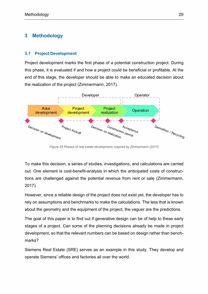
Project development marks the first phase of a potential construction project. During
this phase, it is evaluated if and how a project could be beneficial or profitable. At the
end of this stage, the developer should be able to make an educated decision about
the realization of the project (Zimmermann, 2017).
To make this decision, a series of studies, investigations, and calculations are carried
out. One element is cost-benefit-analysis in which the anticipated costs of construc-
tions are challenged against the potential revenue from rent or sale (Zimmermann,
2017).
However, since a reliable design of the project does not exist yet, the developer has to
rely on assumptions and benchmarks to make the calculations. The less that is known
about the geometry and the equipment of the project, the vaguer are the predictions.
The goal of this paper is to find out if generative design can be of help to these early
stages of a project. Can some of the planning decisions already be made in project
development, so that the relevant numbers can be based on design rather than bench-
marks?
Siemens Real Estate (SRE) serves as an example in this study. They develop and
operate Siemens’ offices and factories all over the world.
3 Methodology
Figure 25 Phases of real estate development; inspired by Zimmermann (2017)
Area development
Project development
Project realization Operation
Developer Operator

Methodology 30
Siemens Real Estate (SRE) is responsible for all of Siemens’ real estate
activities – managing the company’s real estate portfolio, optimizing the
utilization of space, and overseeing the operation of its real estate hold-
ings including all real-estate-related services, as well as having responsi-
bility for leasing and disposing of real estate assets and implementing all
construction projects Siemens-wide.
Siemens Real Estate Website (Siemens, 2019)
The focus of the research is to develop a generative design tool that delivers and opti-
mizes the design of an SRE office building for a specific project. The generated model
should deliver the relevant information for project development and should be opti-
mized to the requirements of both Siemens and specific project conditions.
3.2 Siemens Real Estate Construction Excellence
The Siemens Real Estate Construction Excellence (ConEx) is a technical and archi-
tectural standard developed by SRE.
“Construction Excellence […] is a strategic approach to provide market-ready office
buildings, which are suitable for Siemens and/or other users. Those buildings incorpo-
rate Construction Excellence Standards and Siemens’ branding features.”
(Construction Excellence Office EMEA „Design Principles“, 2015).
It describes the elements that compose a Siemens office building from a single work-
place to complex ventilation systems. Its modular approach is adaptive to different cli-
mate zones, market levels, site conditions, and market-typical office typology.
Methodology 31
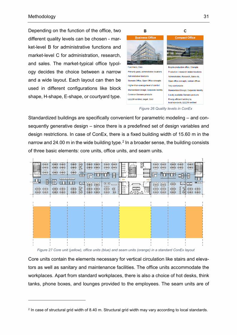
Depending on the function of the office, two
different quality levels can be chosen - mar-
ket-level B for administrative functions and
market-level C for administration, research,
and sales. The market-typical office typol-
ogy decides the choice between a narrow
and a wide layout. Each layout can then be
used in different configurations like block
shape, H-shape, E-shape, or courtyard type.
Standardized buildings are specifically convenient for parametric modeling – and con-
sequently generative design – since there is a predefined set of design variables and
design restrictions. In case of ConEx, there is a fixed building width of 15.60 m in the
narrow and 24.00 m in the wide building type.2 In a broader sense, the building consists
of three basic elements: core units, office units, and seam units.
Core units contain the elements necessary for vertical circulation like stairs and eleva-
tors as well as sanitary and maintenance facilities. The office units accommodate the
workplaces. Apart from standard workplaces, there is also a choice of hot desks, think
tanks, phone boxes, and lounges provided to the employees. The seam units are of
2 In case of structural grid width of 8.40 m. Structural grid width may vary according to local standards.
Figure 26 Quality levels in ConEx
Figure 27 Core unit (yellow), office units (blue) and seam units (orange) in a standard ConEx layout
Methodology 32
the same dimensions as the office units but contain fewer workplaces as they include
a second pair of stairways.
For reasons of fire safety and building services, a sequence of four consecutive office
units must be followed by either a core or a seam unit.
Analogous to ConEx, only the implementation of the block-shaped office is described
in detail in this generative design study. The implementation of other configurations is
discussed in Chapter 7 Discussion and Outlook.
3.3 Parametric Model
“Parametric models used in design are composed of a variety of modules
that combine computation with geometric operations, none of which are
easily differentiable.”
Danil Nagy (The problem of learning, 2017)
As illustrated in 2.1, the parametric model lies at the heart of a generative design study.
Its parameters represent the design variables which ultimately serve as inputs for the
GA. The goal of the optimization ultimately is to find a set of parameter values that
produce the best possible design performance.
The parameters with their individual value range dictate the size of the explorable de-
sign space. They are chosen and defined by the human designer shifting his task from
developing a single object to describing an abstract multidimensional concept (Nagy,
2017c). The parameters should be picked with care since too many inputs might lead
to a design space too big to explore, while too few inputs could exclude a potential
optimum.
In the case of Siemens, two different kinds of inputs must be differentiated: parameters
with fixed values and parameters with variable values. The fixed parameters contain
all the project-specific information. These are:
• Number of employees scheduled to be accommodated in the new office building
(Integer)
• Outline of the property on which the building is developed (Polyline)
• Site entry points, e.g., from parking lot or public streets (Points by coordinates)
• Ground floor height (Double)

Methodology 33
• Regular floor height, usually 3.6 m (Double)
• Grid width, usually 1.2 or 1.35 m (Double)
The parameters that describe design variables serve as input parameters to the GA.
Their value can be changed by the algorithm to generate different designs and explore
the solution space.
The parametric model is implemented in Dynamo, which is a visual programming tool
for design. For that reason, it is best to describe the variables in the order of their
appearance in the script.
Looking at the blank site, the first thing to be determined is the position and the orien-
tation of the building. This is described by a total of four parameters:
• Start Point X-Coordinate (double, range: 0 to 1, step: 0.01)
• Start Point Y-Coordinate (double, range: 0 to 1, step: 0.01)
The start point is described in relation to a bounding
box surrounding the site. At (0/0) the start point
would be located at the lower left corner of the
bounding box (min point), and at (1/1) it lies on the
upper right corner of the bounding box (max point).
• Orientation U-value (double, range: -1 to 1,
step: 0.1)
• Orientation V-value (double, range: -1 to 1,
step: 0.1)
Figure 28 The site polyline defined by corner points in form of coordinates
0 1
1
y
0x
Figure 29 Determination of the start point according to a virtual bounding box
Methodology 34
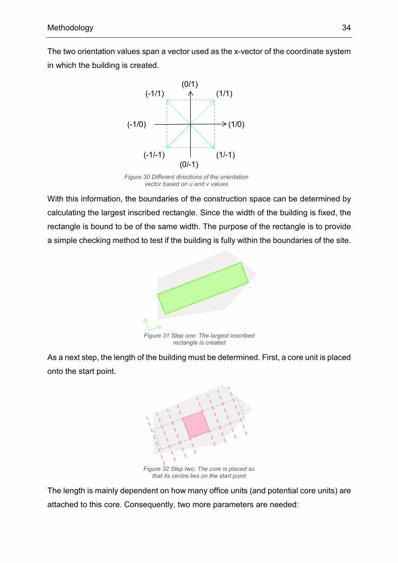
The two orientation values span a vector used as the x-vector of the coordinate system
in which the building is created.
With this information, the boundaries of the construction space can be determined by
calculating the largest inscribed rectangle. Since the width of the building is fixed, the
rectangle is bound to be of the same width. The purpose of the rectangle is to provide
a simple checking method to test if the building is fully within the boundaries of the site.
As a next step, the length of the building must be determined. First, a core unit is placed
onto the start point.
The length is mainly dependent on how many office units (and potential core units) are
attached to this core. Consequently, two more parameters are needed:
Figure 30 Different directions of the orientation vector based on u and v values
Figure 31 Step one: The largest inscribed rectangle is created
Figure 32 Step two: The core is placed so that its centre lies on the start point
(1/0)
(1/1)(0/1)
(-1/1)
(-1/0)
(1/-1)(0/-1)
(-1/-1)
Methodology 35
• Number of units left (integer, range: 2 to ~10, step: 1)
• Number of units right (integer, range: 2 to ~ 10, step: 1)
The upper range limit should be set in accordance with the size of the property. If it is
impossible to fit a building with 20 office units into the site, then the range should be
narrowed to avoid having an unnecessarily big design space.
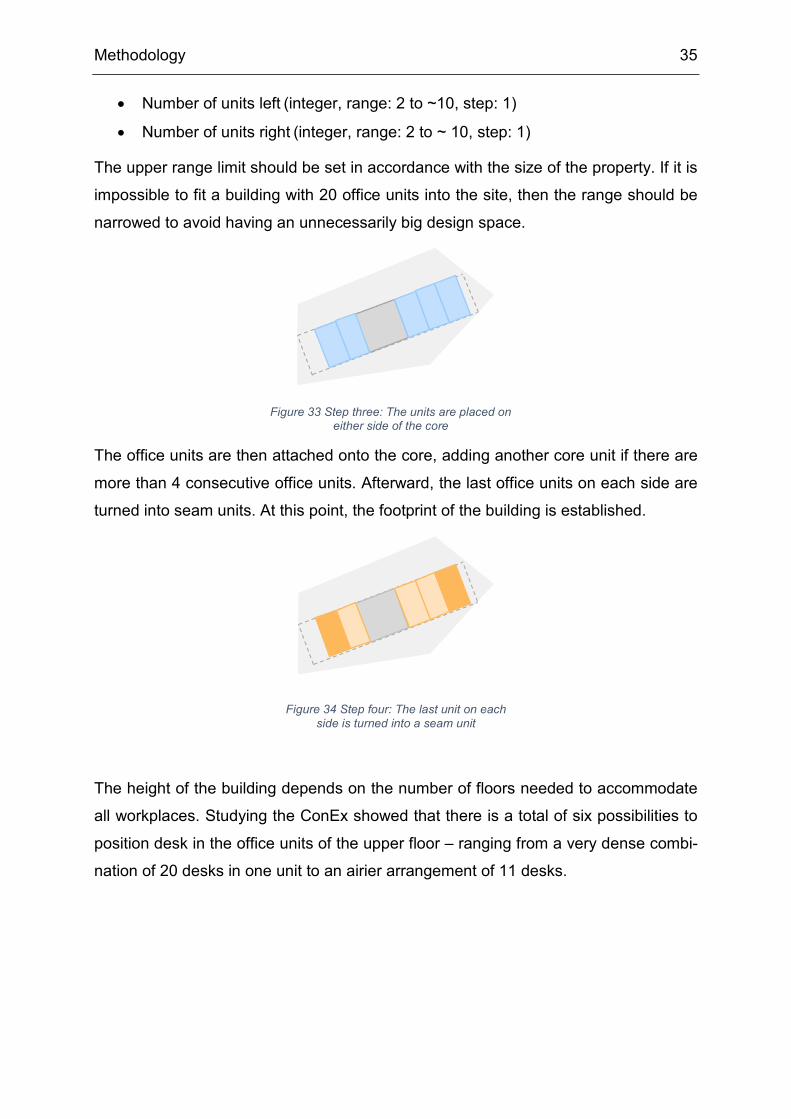
The office units are then attached onto the core, adding another core unit if there are
more than 4 consecutive office units. Afterward, the last office units on each side are
turned into seam units. At this point, the footprint of the building is established.
The height of the building depends on the number of floors needed to accommodate
all workplaces. Studying the ConEx showed that there is a total of six possibilities to
position desk in the office units of the upper floor – ranging from a very dense combi-
nation of 20 desks in one unit to an airier arrangement of 11 desks.
Figure 33 Step three: The units are placed on either side of the core
Figure 34 Step four: The last unit on each side is turned into a seam unit
Methodology 36
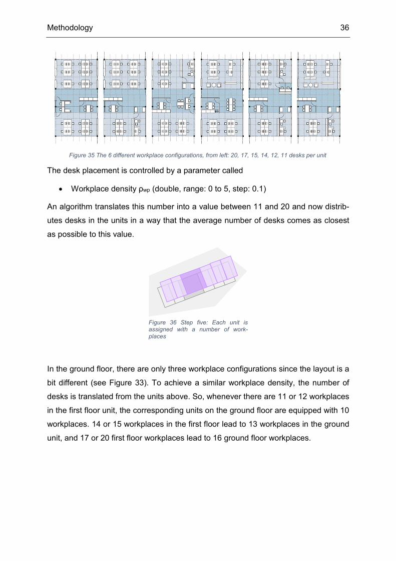
The desk placement is controlled by a parameter called
• Workplace density ρwp (double, range: 0 to 5, step: 0.1)
An algorithm translates this number into a value between 11 and 20 and now distrib-
utes desks in the units in a way that the average number of desks comes as closest
as possible to this value.
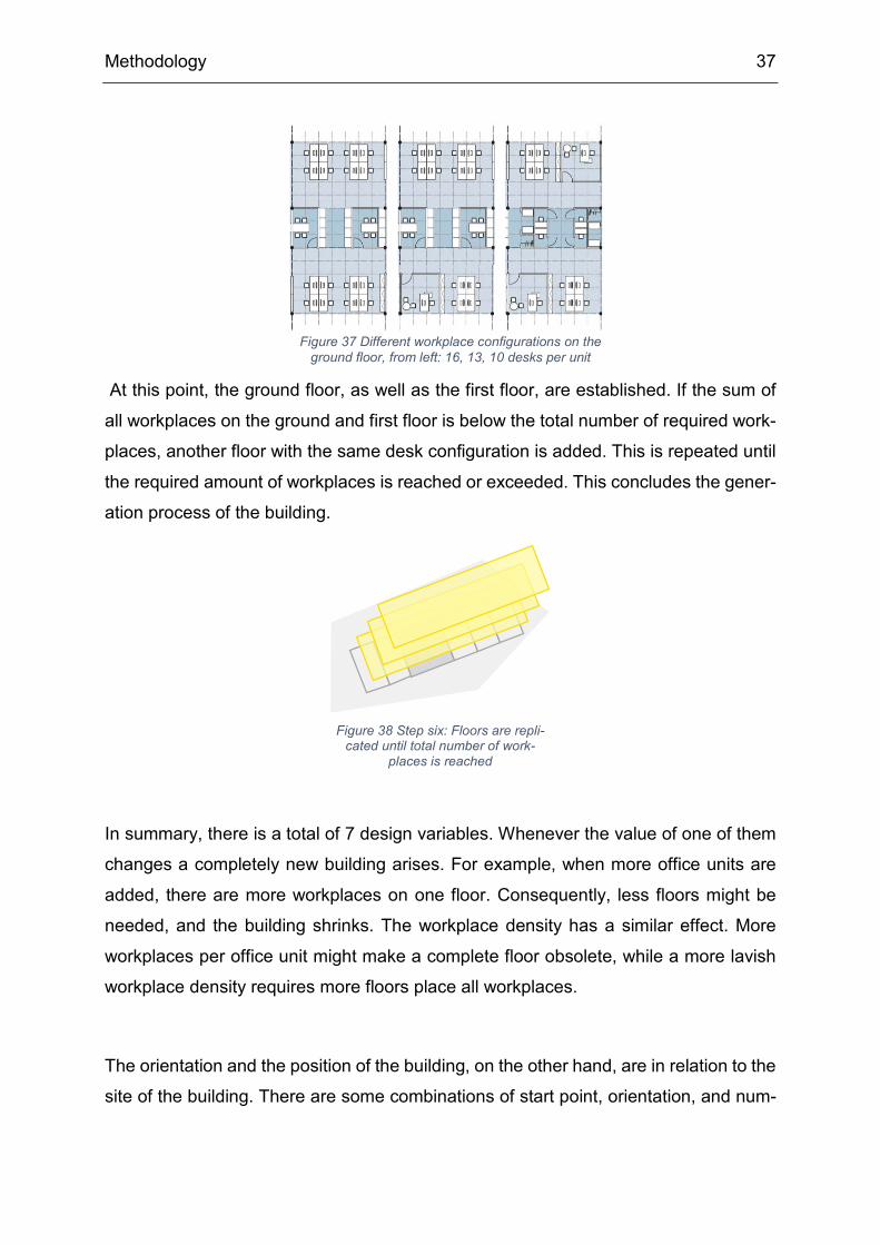
In the ground floor, there are only three workplace configurations since the layout is a
bit different (see Figure 33). To achieve a similar workplace density, the number of
desks is translated from the units above. So, whenever there are 11 or 12 workplaces
in the first floor unit, the corresponding units on the ground floor are equipped with 10
workplaces. 14 or 15 workplaces in the first floor lead to 13 workplaces in the ground
unit, and 17 or 20 first floor workplaces lead to 16 ground floor workplaces.
Figure 35 The 6 different workplace configurations, from left: 20, 17, 15, 14, 12, 11 desks per unit
Figure 36 Step five: Each unit is assigned with a number of work-places
Methodology 37
At this point, the ground floor, as well as the first floor, are established. If the sum of
all workplaces on the ground and first floor is below the total number of required work-
places, another floor with the same desk configuration is added. This is repeated until
the required amount of workplaces is reached or exceeded. This concludes the gener-
ation process of the building.
In summary, there is a total of 7 design variables. Whenever the value of one of them
changes a completely new building arises. For example, when more office units are
added, there are more workplaces on one floor. Consequently, less floors might be
needed, and the building shrinks. The workplace density has a similar effect. More
workplaces per office unit might make a complete floor obsolete, while a more lavish
workplace density requires more floors place all workplaces.
The orientation and the position of the building, on the other hand, are in relation to the
site of the building. There are some combinations of start point, orientation, and num-
Figure 38 Step six: Floors are repli-cated until total number of work-
places is reached
Figure 37 Different workplace configurations on the ground floor, from left: 16, 13, 10 desks per unit

Methodology 38
ber of slices that will lead to invalid designs since the resulting building would be (par-
tially) outside of the property. In these cases, the design will be marked with a bad
value in the evaluation phase to teach the algorithm where to position the building.
Figure 39 Three versions of a model with different parameter values; left: workplace density set to a very low value, hence more floors have to be installed to accommodate all employees; centre: workplace density set to a very low value, some upper floors become obsolete since workplaces are more densely arranged; right: increased number of units on the right, number of floors sinks even more, but model becomes invalid because it exceed the borders of the site

Methodology 39
3.4 Design Goals
The design goals describe what makes a good design. These measures can be sub-
jective to the human decision-maker like aesthetics or comfort, or rational like profit or
the hours of daylight inside of the building. Once the design goals are decided, they
must be paired with indicators that are quantitatively measurable. This allows for the
designs to be compared amongst each other on an objective level.
Together with the project development team of Siemens, 8 design goals were identi-
fied.
1) Comfort Indicator: rentable area/workplace
Calculation: according to ConEx, 8% of floor space is consumed by construction. Of
the remaining area, technical-functional space and vertical traffic space cannot be
rented. Since it is known exactly how much space is consumed by these functions, the
remaining rentable area can be precisely calculated for the different units.
Therefore, rentable area/workplace Ar,w is calculated as:
𝐴𝐴𝑓𝑓,𝑤𝑤 = (48.576 ∗ 𝑖𝑖𝑖𝑖 + 120.5568 ∗ 𝑖𝑖𝑓𝑓 + 98.9568 ∗ 𝑖𝑖𝑠𝑠) ∗ 𝑓𝑓
𝑤𝑤𝑡𝑡𝑓𝑓𝑡𝑡𝑎𝑎𝑎𝑎 ;
nc = number of core units = 1, unless nunit,left or nunit,right < 4;
no = number of office units = (nunit,left -1) + (nunit,right -1);
ns = number of seam units = 2;
f = number of floors;
wtotal = total number of workplaces on all floors (not to be confused with wrequired);
Objective: Maximize – the more rentable area per workplace, the more comfortable for
the working employee
Core unit Office unit Seam unit
total floor area 243.36 131.04 131.04
net floor area 223.8912 120.5568 120.5568
rentable area 48.576 120.5568 98.9568
Table 1 Rentable area in each kind of unit

Methodology 40
2) Functionality
Indicator: meeting area/workplace
Calculation: the meeting rooms are located on the ground floor of the building and
preferable in one bulk on one side of the main core. So, it is assumed that the meeting
rooms are all positioned in the right units on the ground floor. To calculate the meeting
area, the horizontal traffic space must be subtracted from the rentable area. The meet-
ing area/workplace Am,w is calculated as:
𝐴𝐴𝑚𝑚.𝑤𝑤 = (𝑎𝑎𝑚𝑚,𝑟𝑟𝑟𝑟𝑟𝑟𝑟𝑟𝑟𝑟𝑟𝑟𝑟𝑟 ∗ (𝑖𝑖𝑟𝑟𝑛𝑛𝑖𝑖𝑢𝑢,𝑟𝑟𝑖𝑖𝑟𝑟ℎ𝑢𝑢 − 1) + 𝑎𝑎𝑚𝑚,𝑠𝑠𝑟𝑟𝑟𝑟𝑚𝑚)
𝑤𝑤𝑢𝑢𝑡𝑡𝑢𝑢𝑟𝑟𝑟𝑟 ;
am,regular = Meeting area in regular unit = 95.357 m² ;
am,seam = Meeting area in seam unit = 77.357 m² ;
wtotal = total number of workplaces on all floors
Objective: Maximize – the more meeting area / workplace, the more likely there is a
meeting room available when needed
3) Soil sealing
Indicator: footprint
Calculation:
𝐴𝐴𝑓𝑓𝑡𝑡𝑡𝑡𝑢𝑢 = 𝑎𝑎 ∗ 𝑤𝑤 ;
l = length of all units combined;
w = 15,6 m/ 24,00 m;
Objective: Minimize – the smaller the footprint, the less invasive in terms of soil sealing

Methodology 41
4) Cost
Indicator: façade area (because it has the highest price/m² in construction and contrib-
utes to the operating costs in terms of heat loss)
Calculation:
𝐴𝐴𝑓𝑓𝑟𝑟𝑓𝑓𝑟𝑟𝑓𝑓𝑟𝑟 = 2 ∗ 𝑎𝑎 ∗ ℎ + 2 ∗ 𝑤𝑤 ∗ ℎ ;
l = length of all units combined;
w = 15,6 m;
h = hground floor + (f - 1) * hupper floor ;
Objective: Minimize – the less façade area, the lower the construction as well as oper-
ating cost
5) Energy consumption
Indicator: form factor (surface to volume ratio)
Calculation:
𝐹𝐹𝑓𝑓𝑡𝑡𝑟𝑟𝑚𝑚 =2 ∗ 𝑎𝑎 ∗ ℎ + 2 ∗ 𝑤𝑤 ∗ ℎ + 𝑎𝑎 ∗ 𝑤𝑤
𝑎𝑎 ∗ 𝑤𝑤 ∗ ℎ ;
l = length of all units combined;
w = 15,6 m;
h = hground floor + (f - 1) * hupper floor ;
Objective: Minimize – the smaller the form factor, the less energy is consumed by the
building
6) Daylight exploitation
Indicator: orientation in relation to east-west axis
Calculation: the orientation value a ranging from 0 to 1 is used to describe the “east-
west-ness” of the building. At 0 the building is directed from north to south, at 1 the
building is directed from east to west.
Methodology 42
The orientation value a is calculated as:
𝑎𝑎 = 𝑥𝑥
90;
𝑥𝑥 = |90 − 𝛼𝛼| ;
𝛼𝛼 = 𝑖𝑖𝑓𝑓𝑠𝑠−1 �𝑢𝑢 ∗ 𝑣𝑣
|𝑢𝑢| ∗ |𝑣𝑣|� ;
𝑢𝑢 = �10� ;
𝑣𝑣 = 𝑣𝑣𝑖𝑖𝑖𝑖𝑡𝑡𝑓𝑓𝑓𝑓 𝑖𝑖𝑖𝑖𝑡𝑡𝑖𝑖𝑓𝑓𝑑𝑑𝑖𝑖𝑖𝑖𝑖𝑖𝑖𝑖 𝑏𝑏𝑏𝑏 𝑓𝑓𝑓𝑓𝑖𝑖𝑖𝑖𝑖𝑖𝑡𝑡𝑎𝑎𝑡𝑡𝑖𝑖𝑓𝑓𝑖𝑖 𝑓𝑓𝑓𝑓 𝑏𝑏𝑢𝑢𝑖𝑖𝑎𝑎𝑖𝑖𝑖𝑖𝑖𝑖𝑏𝑏 = �𝑓𝑓𝑓𝑓𝑖𝑖𝑖𝑖𝑖𝑖𝑡𝑡𝑎𝑎𝑡𝑡𝑖𝑖𝑓𝑓𝑖𝑖 𝑢𝑢𝑓𝑓𝑓𝑓𝑖𝑖𝑖𝑖𝑖𝑖𝑡𝑡𝑎𝑎𝑡𝑡𝑖𝑖𝑓𝑓𝑖𝑖 𝑣𝑣
� ;
Objective: maximize for W-E-orientation, minimize for N-S-orientation (the objective
varies depending on the latitudinal position)
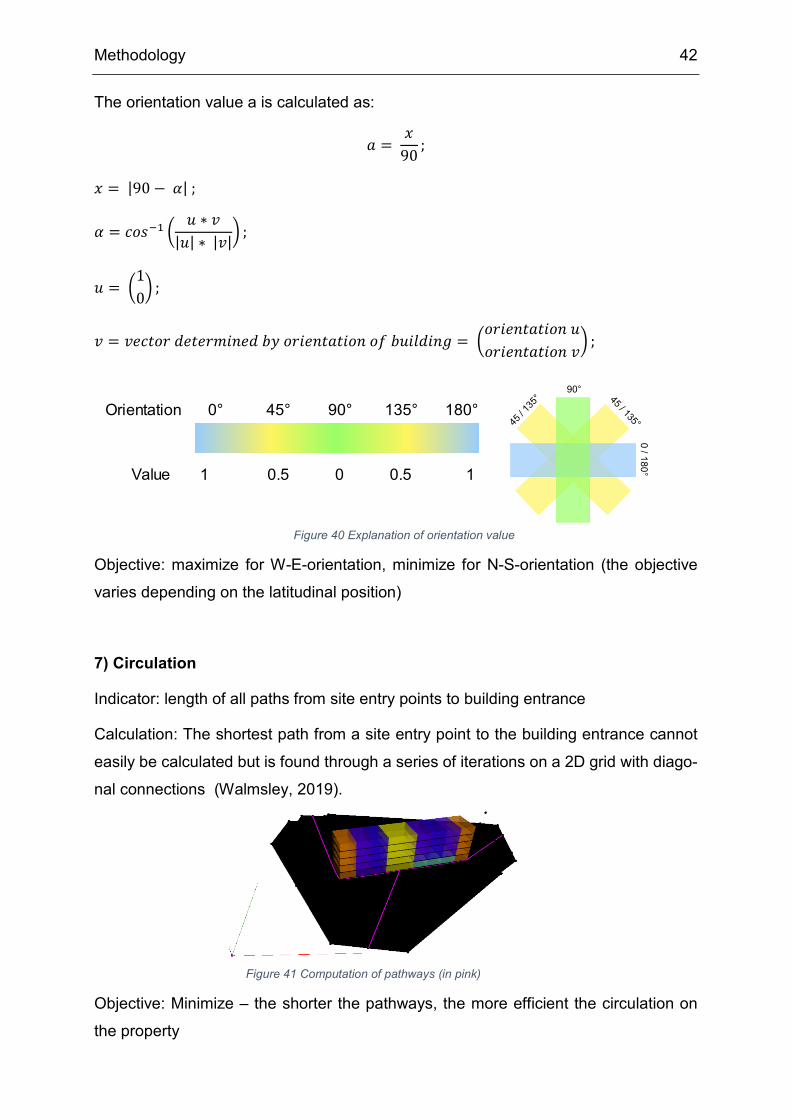
7) Circulation
Indicator: length of all paths from site entry points to building entrance
Calculation: The shortest path from a site entry point to the building entrance cannot
easily be calculated but is found through a series of iterations on a 2D grid with diago-
nal connections (Walmsley, 2019).
Objective: Minimize – the shorter the pathways, the more efficient the circulation on
the property
Figure 40 Explanation of orientation value
Figure 41 Computation of pathways (in pink)
90°
0 / 180°
90°45°0° 135° 180°Orientation
Value 00.51 0.5 1

Methodology 43
8) Workplace accuracy
Indicator: excess workplaces
Calculation:
𝑤𝑤𝑟𝑟𝑒𝑒𝑓𝑓𝑟𝑟𝑠𝑠𝑠𝑠 = 𝑤𝑤𝑢𝑢𝑡𝑡𝑢𝑢𝑟𝑟𝑟𝑟 − 𝑤𝑤𝑟𝑟𝑟𝑟𝑟𝑟𝑟𝑟𝑖𝑖𝑟𝑟𝑟𝑟𝑓𝑓
Objective: Minimize – the fewer excess workplaces, the more accurate to the demand
Methodology 44
3.5 Evolution
To carry out the optimization study, the Dynamo graph was paired with a generative
design tool called Refinery. The design variables of the parametric model serve as
inputs in its optimization algorithm. Refinery docks onto these parameters and changes
their values. It registers the corresponding outcomes and can thereby learn what input
values generate a good design. To optimize the designs, Refinery makes use of
NSGA-II. The number of generations and the population size is defined by the user.
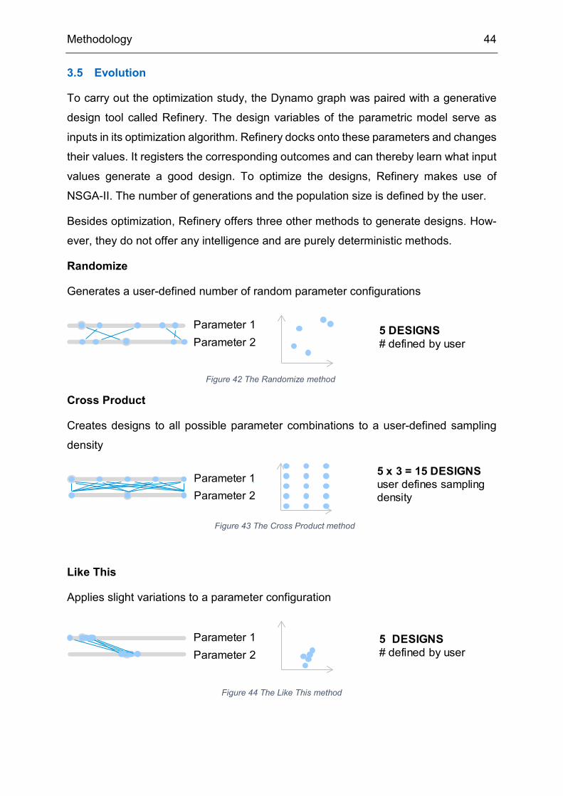
Besides optimization, Refinery offers three other methods to generate designs. How-
ever, they do not offer any intelligence and are purely deterministic methods.
Randomize
Generates a user-defined number of random parameter configurations
Cross Product
Creates designs to all possible parameter combinations to a user-defined sampling
density
Like This
Applies slight variations to a parameter configuration
Figure 44 The Like This method
Parameter 1 5 DESIGNS# defined by userParameter 2
5 x 3 = 15 DESIGNSuser defines sampling density
Parameter 1Parameter 2
Parameter 1Parameter 2
5 DESIGNS# defined by user
Figure 42 The Randomize method
Figure 43 The Cross Product method
Verification 45
4.1 Arithmetic Verification
In order to prove that the Genetic Algorithm (GA) is capable of finding the best solution,
it is tested on a smaller example. A model that resembles a simple trade-off situation
is set up. In this case, it is possible to calculate the optimum of the example, because
the design is composed of a single differentiable function. The result found through
calculation can then be compared to results found through optimization by the GA.
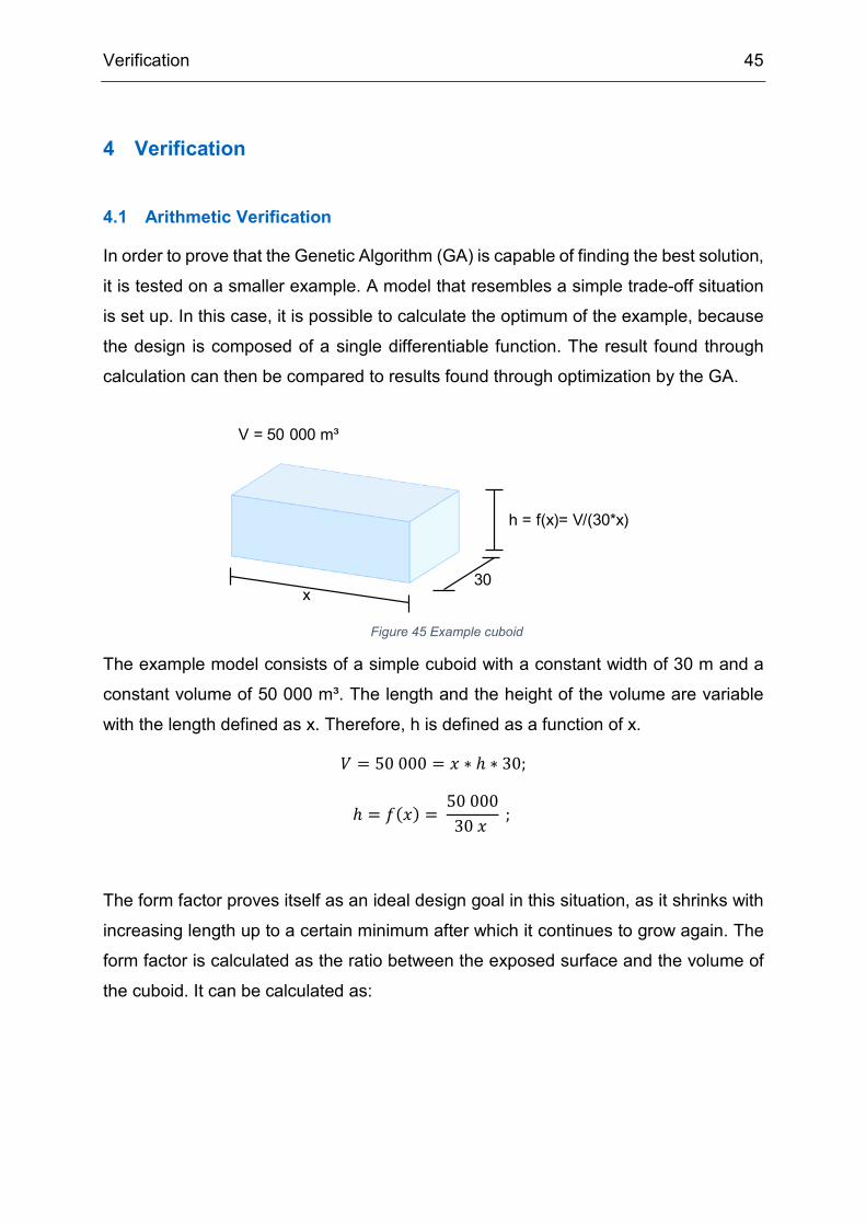
The example model consists of a simple cuboid with a constant width of 30 m and a
constant volume of 50 000 m³. The length and the height of the volume are variable
with the length defined as x. Therefore, h is defined as a function of x.
𝑉𝑉 = 50 000 = 𝑥𝑥 ∗ ℎ ∗ 30;
ℎ = 𝑓𝑓(𝑥𝑥) = 50 00030 𝑥𝑥
;
The form factor proves itself as an ideal design goal in this situation, as it shrinks with
increasing length up to a certain minimum after which it continues to grow again. The
form factor is calculated as the ratio between the exposed surface and the volume of
the cuboid. It can be calculated as:
4 Verification
Figure 45 Example cuboid
x30
h = f(x)= V/(30*x)
V = 50 000 m³
Verification 46
𝐹𝐹𝑓𝑓𝑓𝑓𝑑𝑑 𝑓𝑓𝑎𝑎𝑖𝑖𝑡𝑡𝑓𝑓𝑓𝑓 = 𝑏𝑏(𝑥𝑥) = 2𝑥𝑥ℎ + 2 ∗ 30ℎ + 30𝑥𝑥
𝑉𝑉;
𝑏𝑏(𝑥𝑥) = 2𝑥𝑥ℎ + 60ℎ + 30𝑥𝑥
50 000 ;
= 2𝑥𝑥 �50 000
30𝑥𝑥 � + 60 �50 00030𝑥𝑥 � + 30𝑥𝑥
50 000;
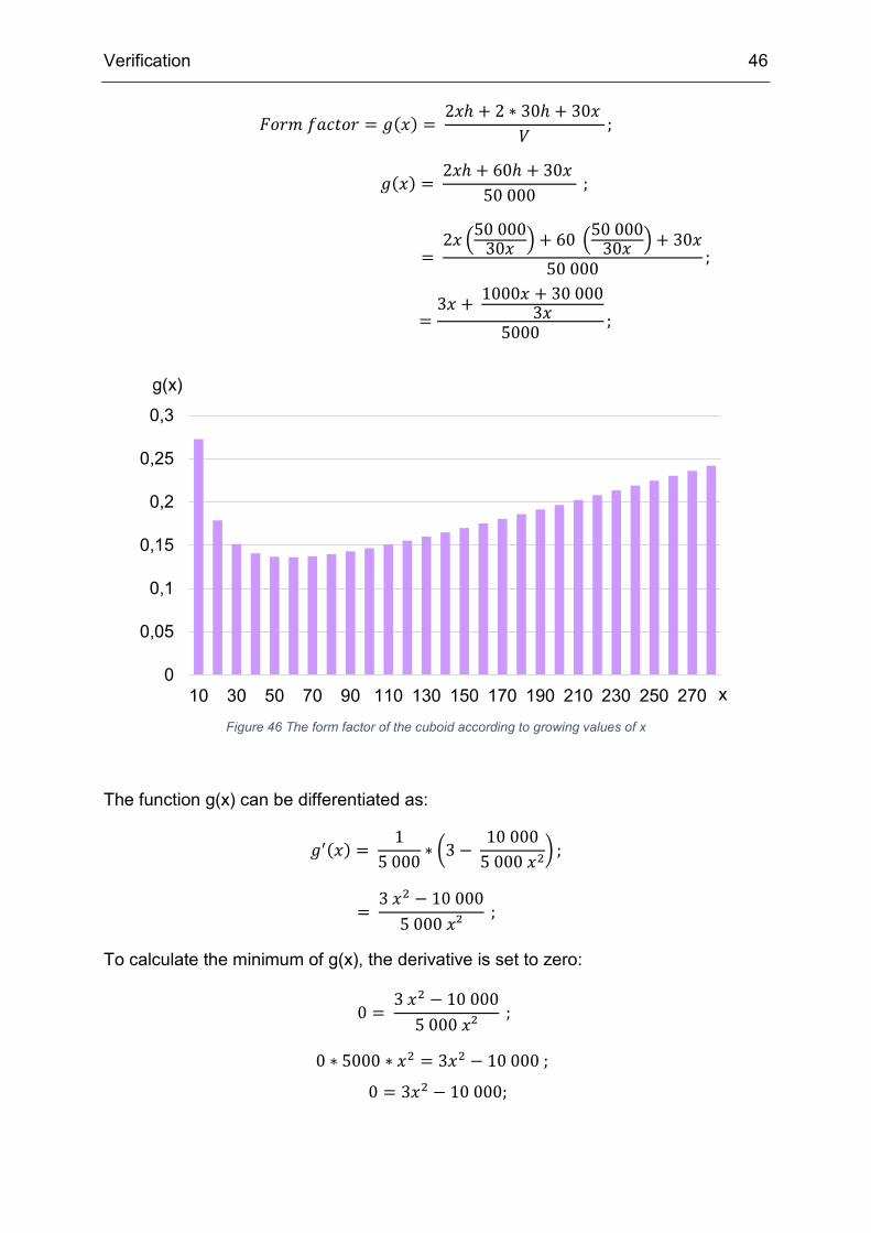
=3𝑥𝑥 + 1000𝑥𝑥 + 30 000
3𝑥𝑥5000
;
The function g(x) can be differentiated as:
𝑏𝑏′(𝑥𝑥) = 1
5 000∗ �3 −
10 0005 000 𝑥𝑥2
� ;
= 3 𝑥𝑥2 − 10 000
5 000 𝑥𝑥² ;
To calculate the minimum of g(x), the derivative is set to zero:
0 = 3 𝑥𝑥2 − 10 000
5 000 𝑥𝑥² ;
0 ∗ 5000 ∗ 𝑥𝑥2 = 3𝑥𝑥2 − 10 000 ;
0 = 3𝑥𝑥2 − 10 000;
Figure 46 The form factor of the cuboid according to growing values of x
0
0,05
0,1
0,15
0,2
0,25
0,3
10 30 50 70 90 110 130 150 170 190 210 230 250 270
g(x)
x
Verification 47
𝑥𝑥2 = 10 000
3 ;
𝑥𝑥 = ±�10 000
3 ;
𝑥𝑥1 = 57.735 = 𝑑𝑑𝑖𝑖𝑖𝑖 ;
( 𝑥𝑥2 = − 57.735 ) ;
𝑏𝑏(57,735) = 0.136 ;
The minimum of g(x) can be found at x = 57.735 with a form factor of 0.136.
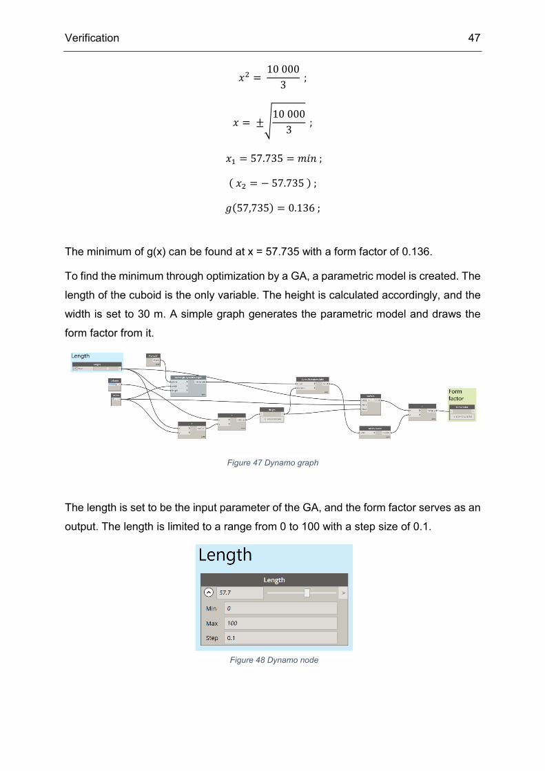
To find the minimum through optimization by a GA, a parametric model is created. The
length of the cuboid is the only variable. The height is calculated accordingly, and the
width is set to 30 m. A simple graph generates the parametric model and draws the
form factor from it.
Figure 47 Dynamo graph
The length is set to be the input parameter of the GA, and the form factor serves as an
output. The length is limited to a range from 0 to 100 with a step size of 0.1.
Figure 48 Dynamo node
Verification 48
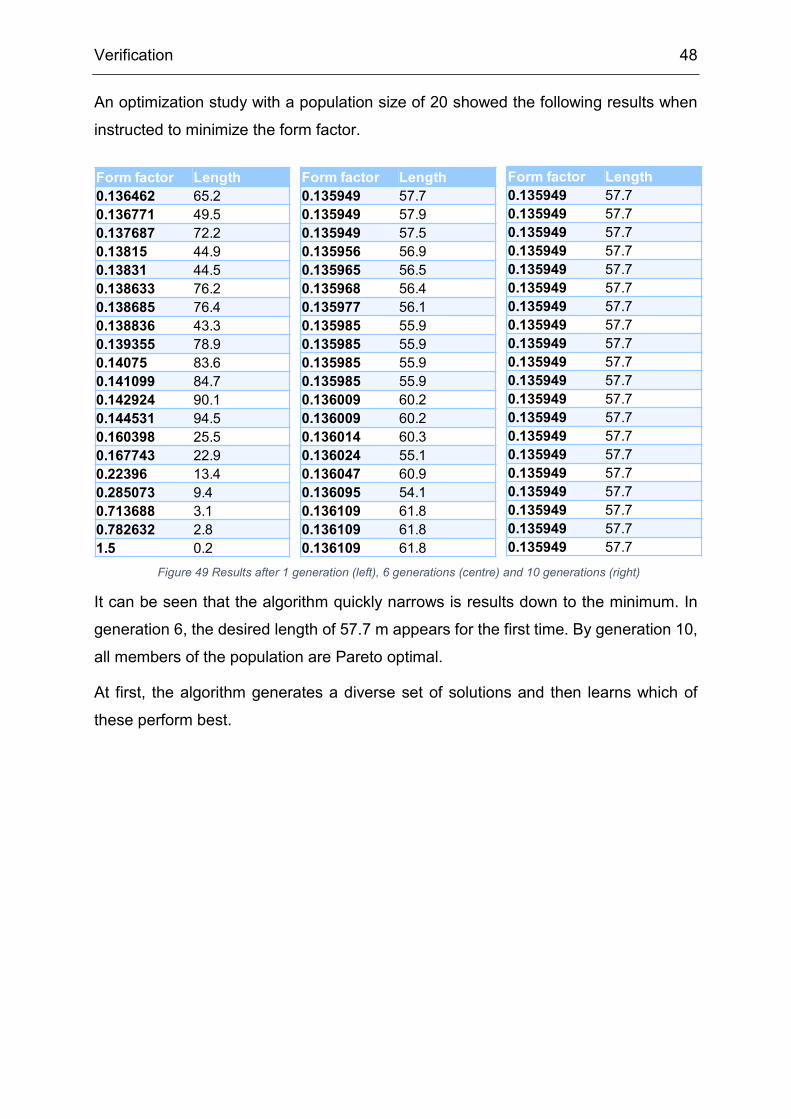
An optimization study with a population size of 20 showed the following results when
instructed to minimize the form factor.
It can be seen that the algorithm quickly narrows is results down to the minimum. In
generation 6, the desired length of 57.7 m appears for the first time. By generation 10,
all members of the population are Pareto optimal.
At first, the algorithm generates a diverse set of solutions and then learns which of
these perform best.
Figure 49 Results after 1 generation (left), 6 generations (centre) and 10 generations (right)
Form factor Length0.136462 65.20.136771 49.50.137687 72.20.13815 44.90.13831 44.50.138633 76.20.138685 76.40.138836 43.30.139355 78.90.14075 83.60.141099 84.70.142924 90.10.144531 94.50.160398 25.50.167743 22.90.22396 13.40.285073 9.40.713688 3.10.782632 2.81.5 0.2
Form factor Length0.135949 57.70.135949 57.90.135949 57.50.135956 56.90.135965 56.50.135968 56.40.135977 56.10.135985 55.90.135985 55.90.135985 55.90.135985 55.90.136009 60.20.136009 60.20.136014 60.30.136024 55.10.136047 60.90.136095 54.10.136109 61.80.136109 61.80.136109 61.8
Form factor Length0.135949 57.70.135949 57.70.135949 57.70.135949 57.70.135949 57.70.135949 57.70.135949 57.70.135949 57.70.135949 57.70.135949 57.70.135949 57.70.135949 57.70.135949 57.70.135949 57.70.135949 57.70.135949 57.70.135949 57.70.135949 57.70.135949 57.70.135949 57.7
Verification 49
4.2 Brute Force Verification
A different approach to verify the results found by the GA would be to generate all
possible solutions in the design space. In the last example, there was only one perfect
solution. However, in design, there is usually a set of Pareto optimal solutions. If the
entire design space is generated, it can be determined if the GA finds all of these so-
lutions. Therefore, a more complex model is needed with functions that are not easily
differentiable.
The cuboid in the second example is fixed in its dimensions with x = 57.7 m. Instead,
by introducing site boundaries, the placement of the cuboid is evaluated. Three varia-
bles are installed:
• Position x
• Position y
• Orientation α
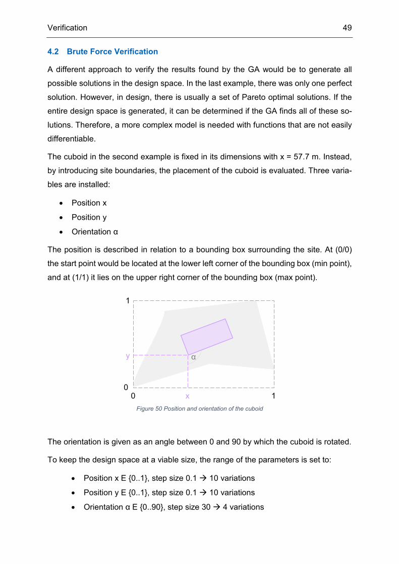
The position is described in relation to a bounding box surrounding the site. At (0/0)
the start point would be located at the lower left corner of the bounding box (min point),
and at (1/1) it lies on the upper right corner of the bounding box (max point).
The orientation is given as an angle between 0 and 90 by which the cuboid is rotated.
To keep the design space at a viable size, the range of the parameters is set to:
• Position x E {0..1}, step size 0.1 10 variations
• Position y E {0..1}, step size 0.1 10 variations
• Orientation α E {0..90}, step size 30 4 variations
Figure 50 Position and orientation of the cuboid 0
01
1
y
x
α
Verification 50
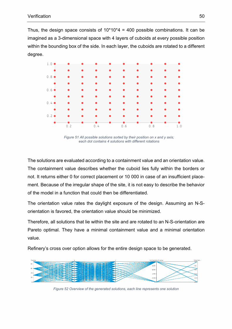
Thus, the design space consists of 10*10*4 = 400 possible combinations. It can be
imagined as a 3-dimensional space with 4 layers of cuboids at every possible position
within the bounding box of the side. In each layer, the cuboids are rotated to a different
degree.
The solutions are evaluated according to a containment value and an orientation value.
The containment value describes whether the cuboid lies fully within the borders or
not. It returns either 0 for correct placement or 10 000 in case of an insufficient place-
ment. Because of the irregular shape of the site, it is not easy to describe the behavior
of the model in a function that could then be differentiated.
The orientation value rates the daylight exposure of the design. Assuming an N-S-
orientation is favored, the orientation value should be minimized.
Therefore, all solutions that lie within the site and are rotated to an N-S-orientation are
Pareto optimal. They have a minimal containment value and a minimal orientation
value.
Refinery’s cross over option allows for the entire design space to be generated.
Figure 51 All possible solutions sorted by their position on x and y axis; each dot contains 4 solutions with different rotations
Figure 52 Overview of the generated solutions, each line represents one solution
Verification 51
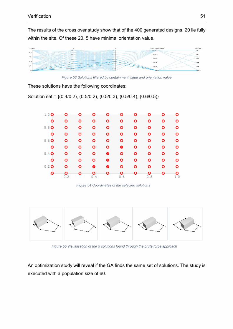
The results of the cross over study show that of the 400 generated designs, 20 lie fully
within the site. Of these 20, 5 have minimal orientation value.
These solutions have the following coordinates:
Solution set = {(0.4/0.2), (0.5/0.2), (0.5/0.3), (0.5/0.4), (0.6/0.5)}
An optimization study will reveal if the GA finds the same set of solutions. The study is
executed with a population size of 60.
Figure 53 Solutions filtered by containment value and orientation value
Figure 54 Coordinates of the selected solutions
Figure 55 Visualisation of the 5 solutions found through the brute force approach

Verification 52
After 6 generations it returns a set of 5 solutions. They match exactly the Pareto optimal
designs found in the brute force approach. Thus, the GA did not only find all the desired
solutions, but it also only needed to generate 360 designs to do so. This is a reduction
of 10% compared to the brute force approach.
It should also be noticed that the actual number of different designs created is much
smaller than 360 since well-performing solutions are passed on through the genera-
tions. Hence the GA found the solution by exploring only a fraction of the design space.
With a larger design space, the effect can be expected to rise significantly.
Figure 57 Visualisation of the 5 solutions found in the optimization study
Figure 56 Solutions found in the optimization study
Implementation 53
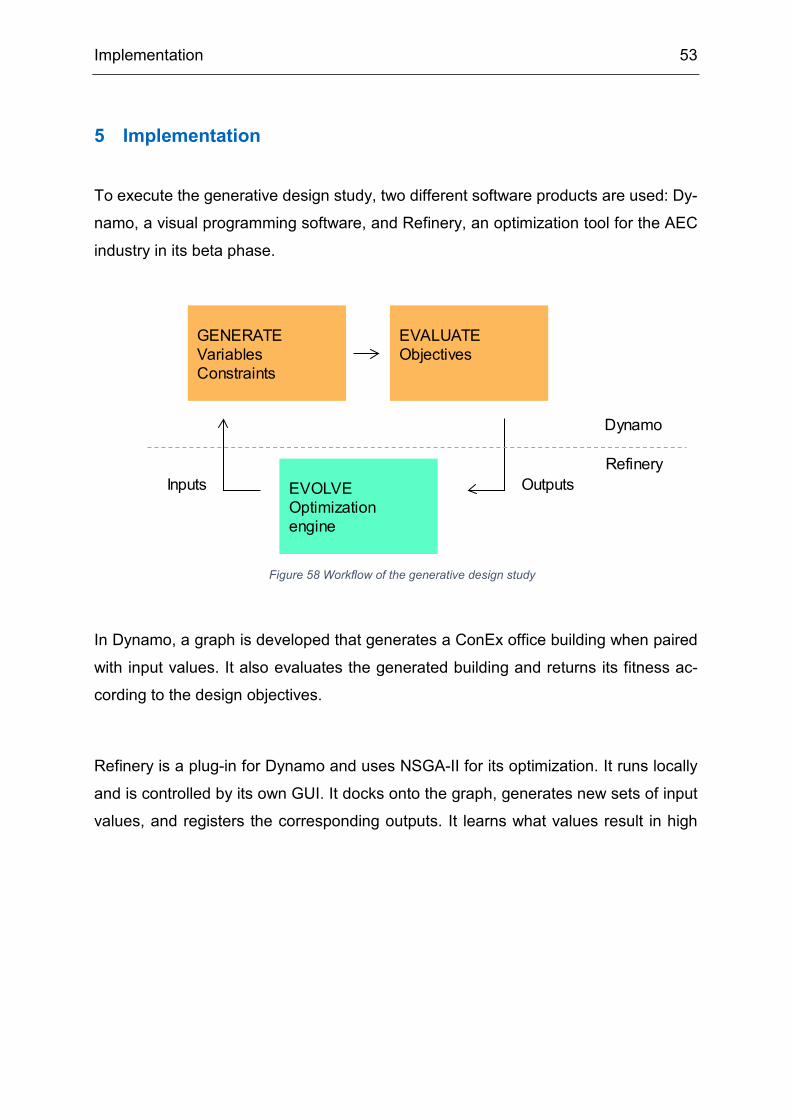
To execute the generative design study, two different software products are used: Dy-
namo, a visual programming software, and Refinery, an optimization tool for the AEC
industry in its beta phase.
In Dynamo, a graph is developed that generates a ConEx office building when paired
with input values. It also evaluates the generated building and returns its fitness ac-
cording to the design objectives.
Refinery is a plug-in for Dynamo and uses NSGA-II for its optimization. It runs locally
and is controlled by its own GUI. It docks onto the graph, generates new sets of input
values, and registers the corresponding outputs. It learns what values result in high
5 Implementation
Figure 58 Workflow of the generative design study
GENERATEVariablesConstraints
EVALUATEObjectives
EVOLVEOptimization engine
Inputs Outputs
Dynamo
Refinery
Implementation 54
performing solutions and optimizes the designs in that direction through crossover and
mutation.
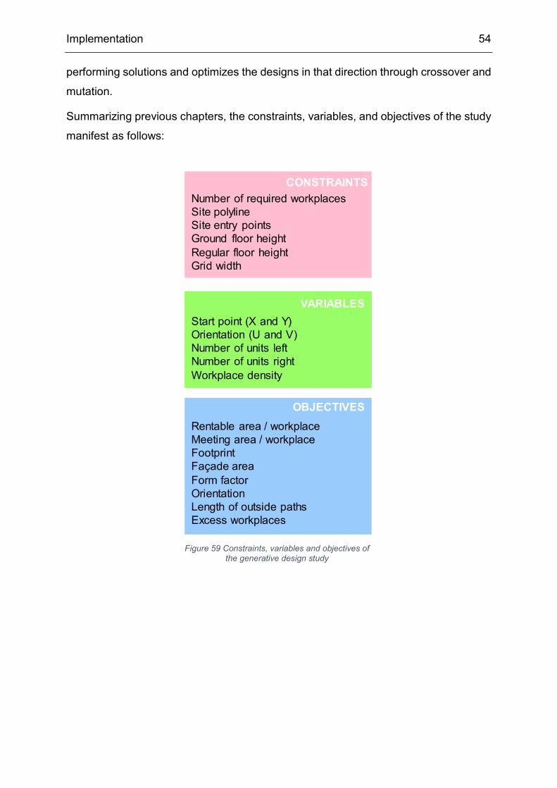
Summarizing previous chapters, the constraints, variables, and objectives of the study
manifest as follows:
Figure 59 Constraints, variables and objectives of the generative design study
Number of required workplacesSite polylineSite entry pointsGround floor heightRegular floor heightGrid width
CONSTRAINTS
Start point (X and Y)Orientation (U and V)Number of units leftNumber of units rightWorkplace density
VARIABLES
Rentable area / workplaceMeeting area / workplaceFootprintFaçade areaForm factorOrientationLength of outside pathsExcess workplaces
OBJECTIVES
Start point (X and Y)Orientation (U and V)Number of units leftNumber of units rightWorkplace density
VARIABLES
Implementation 55
5.1 Dynamo
In visual programming, textual commands are replaced with graphical elements. These
can be combined and manipulated to execute a desired task. In Dynamo, the graphical
elements are called nodes. “Each node performs an operation - sometimes that may
be as simple as storing a number, or it may be a more complex action such as creating
or querying geometry” (The Dynamo Primer, 2018).
Dynamo comes with a choice of pre-installed node libraries. To add further functional-
ity, it offers three options:
• Install more libraries – Nodes developed by other users can be downloaded
and installed through the package manager
• Create custom nodes – In case of a repetitive task, several nodes can be
combined to form a custom node
• Run external script – There are multiple ways to run a textual script in Dy-
namo, the easiest being through a Python node. It allows writing a set of
commands directly in Dynamo as well as process information within the
graph
Dynamo’s node syntax is very convenient for creating visual objects, but it does not
allow recursion and looping. Therefore, combining it with a textual scripting language
like Python facilitates more complex operations.
In the case of the ConEx design problem, a graph must be implemented that produces
a parametric model which is able to explore the entire solution space as well as meas-
ure a solution’s performance. The following two chapters will explain how the graph is
designed to fulfill this task. The graph consists of a total of 380 nodes and 536 connec-
tions. Therefore, the description will only focus on the most important aspects and al-
gorithms of the graph.

Implementation 56
5.1.1 Generate
The workflow to generate a design solution consists of three algorithms and two tests.
A color scheme structures the nodes according to their function. Red marks con-
straints, green indicates variables. Nodes that execute a certain command are sorted
into grey groups, and tests are highlighted in orange.
Largest Inscribed Rectangle
From the start point and the orientation vector, the largest inscribed rectangle can be
created. It marks the area in which the building can spread. It will help to determine
whether the building is placed fully within the borders of the property.
First, the start position is determined. It is defined
in relation to a bounding box surrounding the site
by two variables x, y. Their values vary between
0 and 1.
Start Point
Is rectangle within site?
Orien-tation
# units right
# units left
Workplace density
Create largest inscribed rectangle
Calculate coordinates for
units
Replicate floor until total wp ≥ required wp
Project data
Are all slizeswithin rectangle?
Figure 60 Implementation of the parametric model
Figure 61 The start point is positioned in relation to the bounding box
00
1
1
x
y

Implementation 57
The two orientation variables u and v
span a vector that serves as the x-vector
of the coordinate system, that the building
is built in. To create a rectangle of the
right width, two points are found that are
half the building’s width away from the
start point in positive and negative y-di-
rection.
From these points, vectors are shot in both
positive and negative x-direction until they in-
tersect with the property outline. From the four
intersection points, the two that lie closest to
the start position are chosen and mirrored
onto the opposite vector line so that a rectan-
gle is formed.
After the largest inscribed rectangle is found, a test is carried out to check whether the
rectangle lies fully inside the boundaries of the sit. Through irregular site shapes, there
is a chance that the rectangle includes an area that does not belong to the site. Or if
the start point itself lies outside the site, the algorithm will not be able to form a rectan-
gle at all. In both cases, the test will be marked as failed.
Figure 62 The width of the rectangle is created
Figure 63 The rectangle is closed
Figure 64 Failed construction of the rectangle
vu
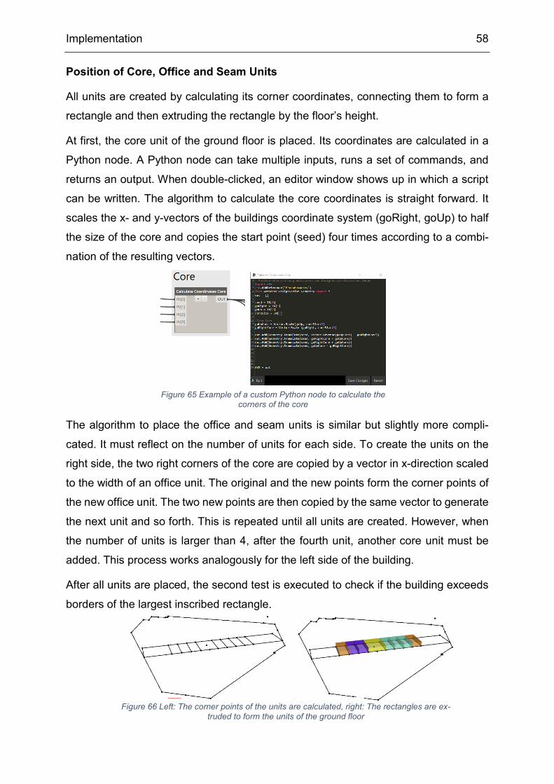
Implementation 58
Position of Core, Office and Seam Units
All units are created by calculating its corner coordinates, connecting them to form a
rectangle and then extruding the rectangle by the floor’s height.
At first, the core unit of the ground floor is placed. Its coordinates are calculated in a
Python node. A Python node can take multiple inputs, runs a set of commands, and
returns an output. When double-clicked, an editor window shows up in which a script
can be written. The algorithm to calculate the core coordinates is straight forward. It
scales the x- and y-vectors of the buildings coordinate system (goRight, goUp) to half
the size of the core and copies the start point (seed) four times according to a combi-
nation of the resulting vectors.
The algorithm to place the office and seam units is similar but slightly more compli-
cated. It must reflect on the number of units for each side. To create the units on the
right side, the two right corners of the core are copied by a vector in x-direction scaled
to the width of an office unit. The original and the new points form the corner points of
the new office unit. The two new points are then copied by the same vector to generate
the next unit and so forth. This is repeated until all units are created. However, when
the number of units is larger than 4, after the fourth unit, another core unit must be
added. This process works analogously for the left side of the building.
After all units are placed, the second test is executed to check if the building exceeds
borders of the largest inscribed rectangle.
Figure 65 Example of a custom Python node to calculate the corners of the core
Figure 66 Left: The corner points of the units are calculated, right: The rectangles are ex-truded to form the units of the ground floor
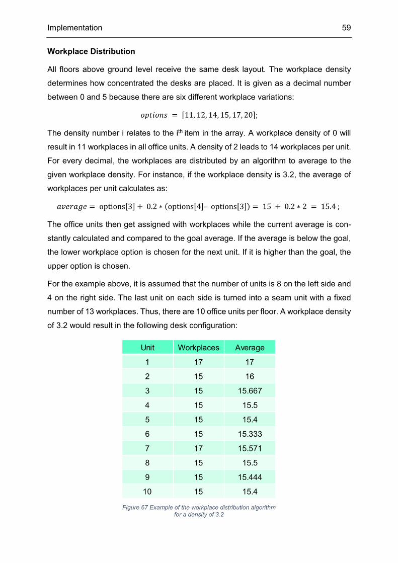
Implementation 59
Workplace Distribution
All floors above ground level receive the same desk layout. The workplace density
determines how concentrated the desks are placed. It is given as a decimal number
between 0 and 5 because there are six different workplace variations:
𝑓𝑓𝑜𝑜𝑡𝑡𝑖𝑖𝑓𝑓𝑖𝑖𝑠𝑠 = [11, 12, 14, 15, 17, 20];
The density number i relates to the ith item in the array. A workplace density of 0 will
result in 11 workplaces in all office units. A density of 2 leads to 14 workplaces per unit.
For every decimal, the workplaces are distributed by an algorithm to average to the
given workplace density. For instance, if the workplace density is 3.2, the average of
workplaces per unit calculates as:
𝑎𝑎𝑣𝑣𝑖𝑖𝑓𝑓𝑎𝑎𝑏𝑏𝑖𝑖 = options[3] + 0.2 ∗ (options[4]– options[3]) = 15 + 0.2 ∗ 2 = 15.4 ;
The office units then get assigned with workplaces while the current average is con-
stantly calculated and compared to the goal average. If the average is below the goal,
the lower workplace option is chosen for the next unit. If it is higher than the goal, the
upper option is chosen.
For the example above, it is assumed that the number of units is 8 on the left side and
4 on the right side. The last unit on each side is turned into a seam unit with a fixed
number of 13 workplaces. Thus, there are 10 office units per floor. A workplace density
of 3.2 would result in the following desk configuration:
Figure 67 Example of the workplace distribution algorithm for a density of 3.2
Unit Workplaces Average
1 17 17
2 15 16
3 15 15.667
4 15 15.5
5 15 15.4
6 15 15.333
7 17 15.571
8 15 15.5
9 15 15.444
10 15 15.4

Implementation 60
Since the layout of the ground floor is different from the upper floors, there are only
three workplace configurations:
𝑓𝑓𝑜𝑜𝑡𝑡𝑖𝑖𝑓𝑓𝑖𝑖𝑠𝑠 = [10, 13, 16];
To achieve a similar workplace density, the number of desks is translated from the
units above. So, whenever there are 11 or 12 workplaces in the first floor unit, the
corresponding units on the ground floor are equipped with 10 workplaces. 14 or 15
workplaces in the first floor lead to 13 workplaces in the ground unit, and 17 or 20 first
floor workplaces lead to 16 ground floor workplaces. It should be kept in mind that on
the ground floor only the units on the left side are equipped with workplaces since the
units on the right are turned into meeting rooms.
In the above example, this would lead to the following workplace distribution in the 7
office units of the ground floor: [16, 13, 13, 13, 13, 13, 16]. The seam units on the
ground floor hold 8 workplaces.
Consequently, there are 180 workplaces on the first floor and 105 workplaces on the
ground floor. This results in a current total of 285 workplaces.
The first floor is replicated until the total number of required workplaces is reached.
Assuming the building is developed to contain 600 workplaces, this adds two more
floors to the building resulting in a total of 645 workplaces.
All units are colored according to their function. Cores appear yellow, and seam units
are depicted in orange. The color of office units varies according to the number of
workplaces they accommodate from pink to blue. Office units with meeting rooms ap-
pear in turquoise.
This concludes the generation process for the different design solutions.
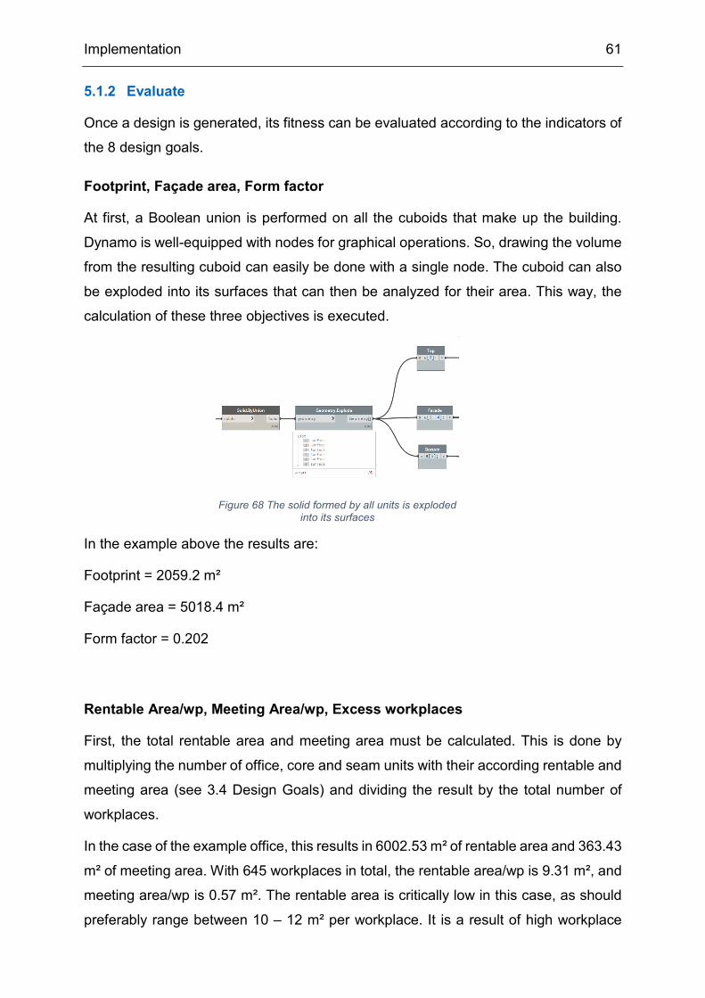
Implementation 61
5.1.2 Evaluate
Once a design is generated, its fitness can be evaluated according to the indicators of
the 8 design goals.
Footprint, Façade area, Form factor
At first, a Boolean union is performed on all the cuboids that make up the building.
Dynamo is well-equipped with nodes for graphical operations. So, drawing the volume
from the resulting cuboid can easily be done with a single node. The cuboid can also
be exploded into its surfaces that can then be analyzed for their area. This way, the
calculation of these three objectives is executed.
In the example above the results are:
Footprint = 2059.2 m²
Façade area = 5018.4 m²
Form factor = 0.202
Rentable Area/wp, Meeting Area/wp, Excess workplaces
First, the total rentable area and meeting area must be calculated. This is done by
multiplying the number of office, core and seam units with their according rentable and
meeting area (see 3.4 Design Goals) and dividing the result by the total number of
workplaces.
In the case of the example office, this results in 6002.53 m² of rentable area and 363.43
m² of meeting area. With 645 workplaces in total, the rentable area/wp is 9.31 m², and
meeting area/wp is 0.57 m². The rentable area is critically low in this case, as should
preferably range between 10 – 12 m² per workplace. It is a result of high workplace
Figure 68 The solid formed by all units is exploded into its surfaces

Implementation 62
density. When the workplace density is changed to 0.6, for instance, the rentable
area/wp rises to 11.83 m². However, since another floor has to be added to accommo-
date all workplaces, the façade area rises to 6081.12 m².
Circulation
To implement pathfinding, custom nodes from a package called Space Analysis were
used. They work with a SpaceLattice object, which is a 2D grid with diagonal connec-
tions. The building is set to be a barrier on the grid, which means paths have to go
around it. An object called PathField allows for multiple routes to one endpoint to be
calculated at the cost of a single calculation. The site entry points act as the start points
to these routes.
Figure 69 When the workplace density is changed to a lower value more floors are needed
Figure 71 Custom nodes from the Space Analysis package
Figure 70 Path finding in Dynamo
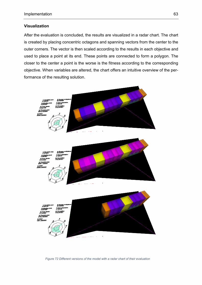
Implementation 63
Visualization
After the evaluation is concluded, the results are visualized in a radar chart. The chart
is created by placing concentric octagons and spanning vectors from the center to the
outer corners. The vector is then scaled according to the results in each objective and
used to place a point at its end. These points are connected to form a polygon. The
closer to the center a point is the worse is the fitness according to the corresponding
objective. When variables are altered, the chart offers an intuitive overview of the per-
formance of the resulting solution.
Figure 72 Different versions of the model with a radar chart of their evaluation
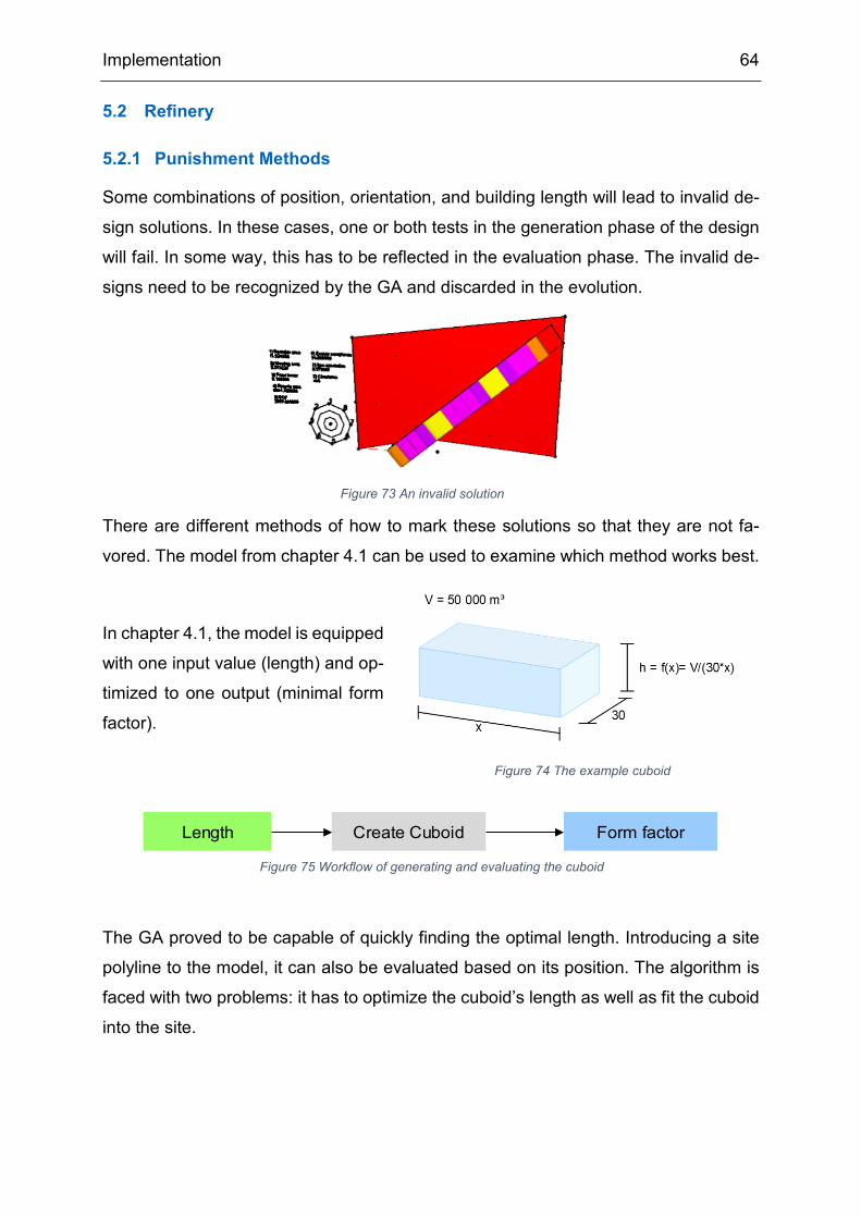
Implementation 64
5.2 Refinery
5.2.1 Punishment Methods
Some combinations of position, orientation, and building length will lead to invalid de-
sign solutions. In these cases, one or both tests in the generation phase of the design
will fail. In some way, this has to be reflected in the evaluation phase. The invalid de-
signs need to be recognized by the GA and discarded in the evolution.
There are different methods of how to mark these solutions so that they are not fa-
vored. The model from chapter 4.1 can be used to examine which method works best.
In chapter 4.1, the model is equipped
with one input value (length) and op-
timized to one output (minimal form
factor).
The GA proved to be capable of quickly finding the optimal length. Introducing a site
polyline to the model, it can also be evaluated based on its position. The algorithm is
faced with two problems: it has to optimize the cuboid’s length as well as fit the cuboid
into the site.
Figure 73 An invalid solution
Figure 74 The example cuboid
Figure 75 Workflow of generating and evaluating the cuboid
Length Create Cuboid Form factor
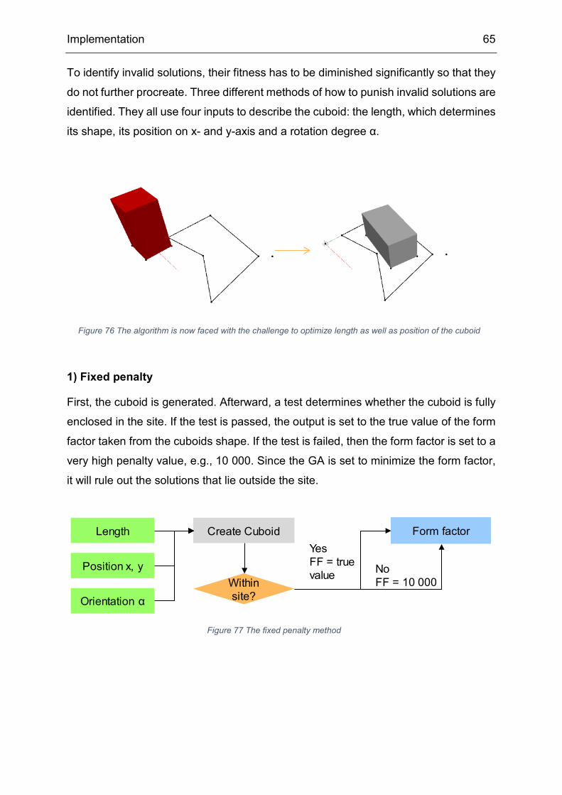
Implementation 65
To identify invalid solutions, their fitness has to be diminished significantly so that they
do not further procreate. Three different methods of how to punish invalid solutions are
identified. They all use four inputs to describe the cuboid: the length, which determines
its shape, its position on x- and y-axis and a rotation degree α.
1) Fixed penalty
First, the cuboid is generated. Afterward, a test determines whether the cuboid is fully
enclosed in the site. If the test is passed, the output is set to the true value of the form
factor taken from the cuboids shape. If the test is failed, then the form factor is set to a
very high penalty value, e.g., 10 000. Since the GA is set to minimize the form factor,
it will rule out the solutions that lie outside the site.
Figure 76 The algorithm is now faced with the challenge to optimize length as well as position of the cuboid
Figure 77 The fixed penalty method
Length Create Cuboid Form factor
Position x, y
Orientation αWithin site?
Yes FF = true value No
FF = 10 000
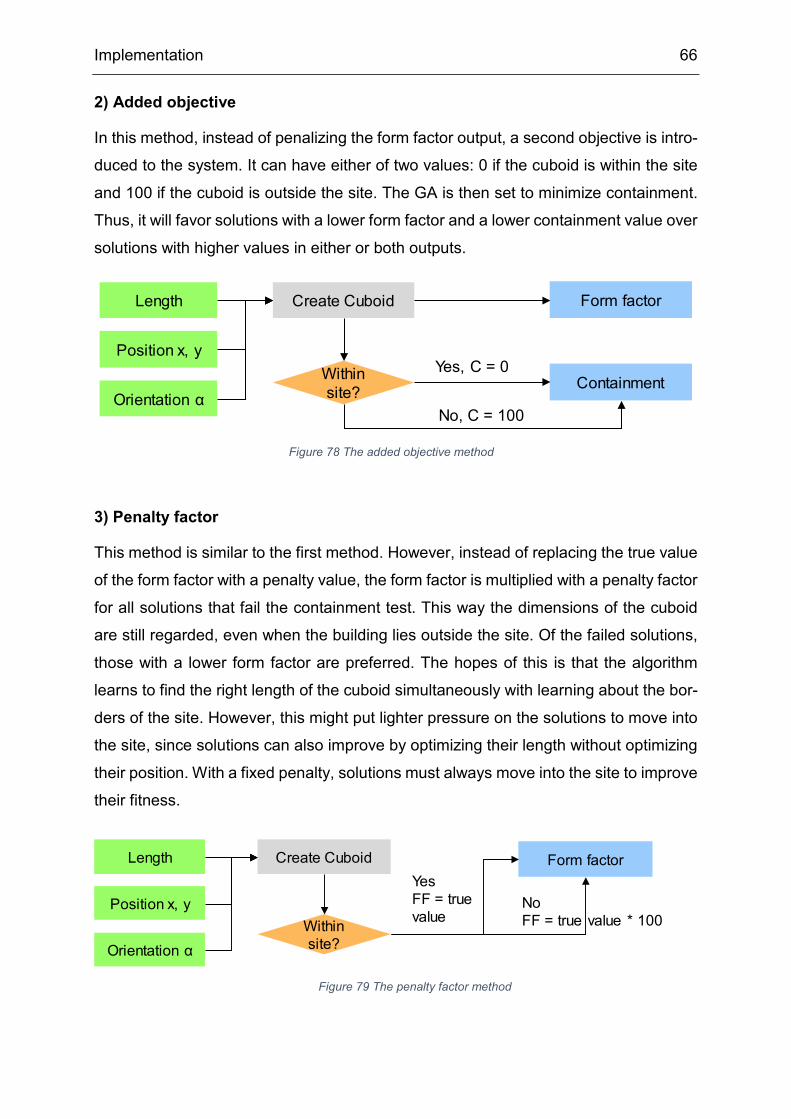
Implementation 66
2) Added objective
In this method, instead of penalizing the form factor output, a second objective is intro-
duced to the system. It can have either of two values: 0 if the cuboid is within the site
and 100 if the cuboid is outside the site. The GA is then set to minimize containment.
Thus, it will favor solutions with a lower form factor and a lower containment value over
solutions with higher values in either or both outputs.
3) Penalty factor
This method is similar to the first method. However, instead of replacing the true value
of the form factor with a penalty value, the form factor is multiplied with a penalty factor
for all solutions that fail the containment test. This way the dimensions of the cuboid
are still regarded, even when the building lies outside the site. Of the failed solutions,
those with a lower form factor are preferred. The hopes of this is that the algorithm
learns to find the right length of the cuboid simultaneously with learning about the bor-
ders of the site. However, this might put lighter pressure on the solutions to move into
the site, since solutions can also improve by optimizing their length without optimizing
their position. With a fixed penalty, solutions must always move into the site to improve
their fitness.
Figure 78 The added objective method
Figure 79 The penalty factor method
Length Create Cuboid Form factor
Position x, y
Orientation αWithin site? Containment
Yes, C = 0
No, C = 100
Length Create Cuboid Form factor
Position x, y
Orientation αWithin site?
Yes FF = true value
NoFF = true value * 100

Implementation 67
For each of the method, a graph is implemented, and a generative design study is
carried out in Refinery. They are compared by the number of generations it takes until
all members of a population of a) 20 and b) 100 are within the site and have the optimal
length of 57.7 m (minimal form factor, see Chapter 4 Verification).
For the basic script with no regards to the site the GA takes
a) 9 generations
b) 8 generations
to optimize the design to minimal form factor.
The results for the three different punishment methods are:
1) Fixed penalty
a) 71 generations
b) 16 generations
2) Second objective
a) 15 generations
b) 12 generations
3) Penalty factor
a) 26 generations
b) 17 generations
Figure 80 Number of generations each method needed to optimize its solutions
0
10
20
30
40
50
60
70
80
Basic script Fixed penalty Second objective Penalty factor
a) p = 20 b) p = 100
Implementation 68
The best performance is achieved by the second method. Even with a small population
size, it was able to optimize the entire population within a low number of generations
by introducing a second objective. However, translating the effect to the ConEx study
might be difficult, since there are eight design goals. Introducing a containment objec-
tive might not add the same kind of pressure on the optimization. The fixed penalty-
method performed bad for the small population size because the algorithm cannot de-
tect any changes in the output values unless there is a design within the site. Therefore,
when none of the solutions lie within the site in the first generations, it cannot learn
anything about which length produces a good form factor. It depends on the randomi-
zation of the first generation and the mutation afterward how fast the designs find its
way into the site. With a larger population size the chances of a valid solution within
the first generations rise, and then the algorithm performs decently because the selec-
tion pressure is quite high as the output of the valid solutions is so significantly lower
compared to invalid solutions.
The penalty factor method performs better than the fixed penalty method for a smaller
population size because of its ability to simultaneously learn about sizes and site limits.
However, its performance does not increase significantly when introduced to a bigger
population size. This might be due to the selection pressure not being high enough.
Depending on the value of the penalty factor itself, it can happen that an invalid solution
with a low form factor is favored over a solution within the site but with a high form
factor.
A clear decision as to which method suits the ConEx optimization problem best is hard
to draw from these results. Further experiments on the actual problem are needed to
answer the questions:
- Does introducing a single objective concerning containment add enough signif-
icance to the position to cancel out invalid solutions?
- Does introducing a fixed penalty add too much pressure to the system, making
it impossible for the GA to learn?
- Does a penalty factor put enough pressure on the GA to favor solutions within
the site?
The goal is to rule out the invalid solutions as soon as they occur so that the optimiza-
tion can focus mainly on improving good solutions.

Implementation 69
Therefore, the three punishment methods are tested on the ConEx optimization graph
in a short run of 5 generations to see which method is able to remove invalid solutions
as quickly as possible. The three optimizations start with the same set of solutions for
the first population. It consists of 200 solutions, of which only 6 are valid (3%). After 5
generations, it is counted how well the solutions propagated. The results are as follows:
1) Fixed penalty: 127/200 (63.5%)
2) Added objective: 14/200 (7%)
3) Penalty factor: 163/200 (81.5%)
The results of the second method increased to 28/200 (14%) when the containment
output was duplicated four times, so it would have a bigger weight on the evolution
compared to the other 8 objectives. However, it can be seen that the factoring method
performed best at removing invalid solutions. When comparing the quality of the valid
solutions, the overall fitness of the penalty factor method population was slightly higher
than the population of the fixed penalty method. Therefore, the penalty factor method
was chosen for the ConEx optimization. Fine-tuning the factors can improve the effects
of the method even further. A penalty factor of 100 for objectives that are supposed to
be minimized and -100 for objectives to be maximized proved to enhance performance.
5.2.2 Population Size, Number of Generations and other NSGA-II settings
When Refinery is installed in Dynamo, it adds the functionality to define nodes in the
graph as inputs and outputs of the optimization.
Figure 81 Inputs and outputs in the Dynamo user interface
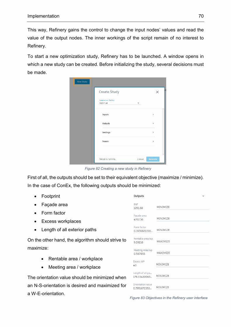
Implementation 70
This way, Refinery gains the control to change the input nodes’ values and read the
value of the output nodes. The inner workings of the script remain of no interest to
Refinery.
To start a new optimization study, Refinery has to be launched. A window opens in
which a new study can be created. Before initializing the study, several decisions must
be made.
First of all, the outputs should be set to their equivalent objective (maximize / minimize).
In the case of ConEx, the following outputs should be minimized:
• Footprint
• Façade area
• Form factor
• Excess workplaces
• Length of all exterior paths
On the other hand, the algorithm should strive to
maximize:
• Rentable area / workplace
• Meeting area / workplace
The orientation value should be minimized when
an N-S-orientation is desired and maximized for
a W-E-orientation.
Figure 82 Creating a new study in Refinery
Figure 83 Objectives in the Refinery user interface
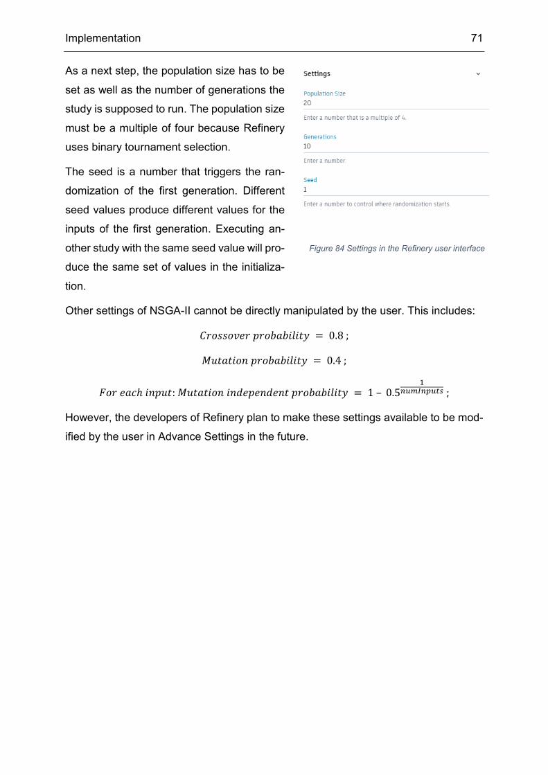
Implementation 71
As a next step, the population size has to be
set as well as the number of generations the
study is supposed to run. The population size
must be a multiple of four because Refinery
uses binary tournament selection.
The seed is a number that triggers the ran-
domization of the first generation. Different
seed values produce different values for the
inputs of the first generation. Executing an-
other study with the same seed value will pro-
duce the same set of values in the initializa-
tion.
Other settings of NSGA-II cannot be directly manipulated by the user. This includes:
𝐶𝐶𝑓𝑓𝑓𝑓𝑠𝑠𝑠𝑠𝑓𝑓𝑣𝑣𝑖𝑖𝑓𝑓 𝑜𝑜𝑓𝑓𝑓𝑓𝑏𝑏𝑎𝑎𝑏𝑏𝑖𝑖𝑎𝑎𝑖𝑖𝑡𝑡𝑏𝑏 = 0.8 ;
𝑀𝑀𝑢𝑢𝑡𝑡𝑎𝑎𝑡𝑡𝑖𝑖𝑓𝑓𝑖𝑖 𝑜𝑜𝑓𝑓𝑓𝑓𝑏𝑏𝑎𝑎𝑏𝑏𝑖𝑖𝑎𝑎𝑖𝑖𝑡𝑡𝑏𝑏 = 0.4 ;
𝐹𝐹𝑓𝑓𝑓𝑓 𝑖𝑖𝑎𝑎𝑖𝑖ℎ 𝑖𝑖𝑖𝑖𝑜𝑜𝑢𝑢𝑡𝑡: 𝑀𝑀𝑢𝑢𝑡𝑡𝑎𝑎𝑡𝑡𝑖𝑖𝑓𝑓𝑖𝑖 𝑖𝑖𝑖𝑖𝑖𝑖𝑖𝑖𝑜𝑜𝑖𝑖𝑖𝑖𝑖𝑖𝑖𝑖𝑖𝑖𝑡𝑡 𝑜𝑜𝑓𝑓𝑓𝑓𝑏𝑏𝑎𝑎𝑏𝑏𝑖𝑖𝑎𝑎𝑖𝑖𝑡𝑡𝑏𝑏 = 1 – 0.51
𝑛𝑛𝑟𝑟𝑚𝑚𝑛𝑛𝑛𝑛𝑛𝑛𝑟𝑟𝑢𝑢𝑠𝑠 ;
However, the developers of Refinery plan to make these settings available to be mod-
ified by the user in Advance Settings in the future.
Figure 84 Settings in the Refinery user interface
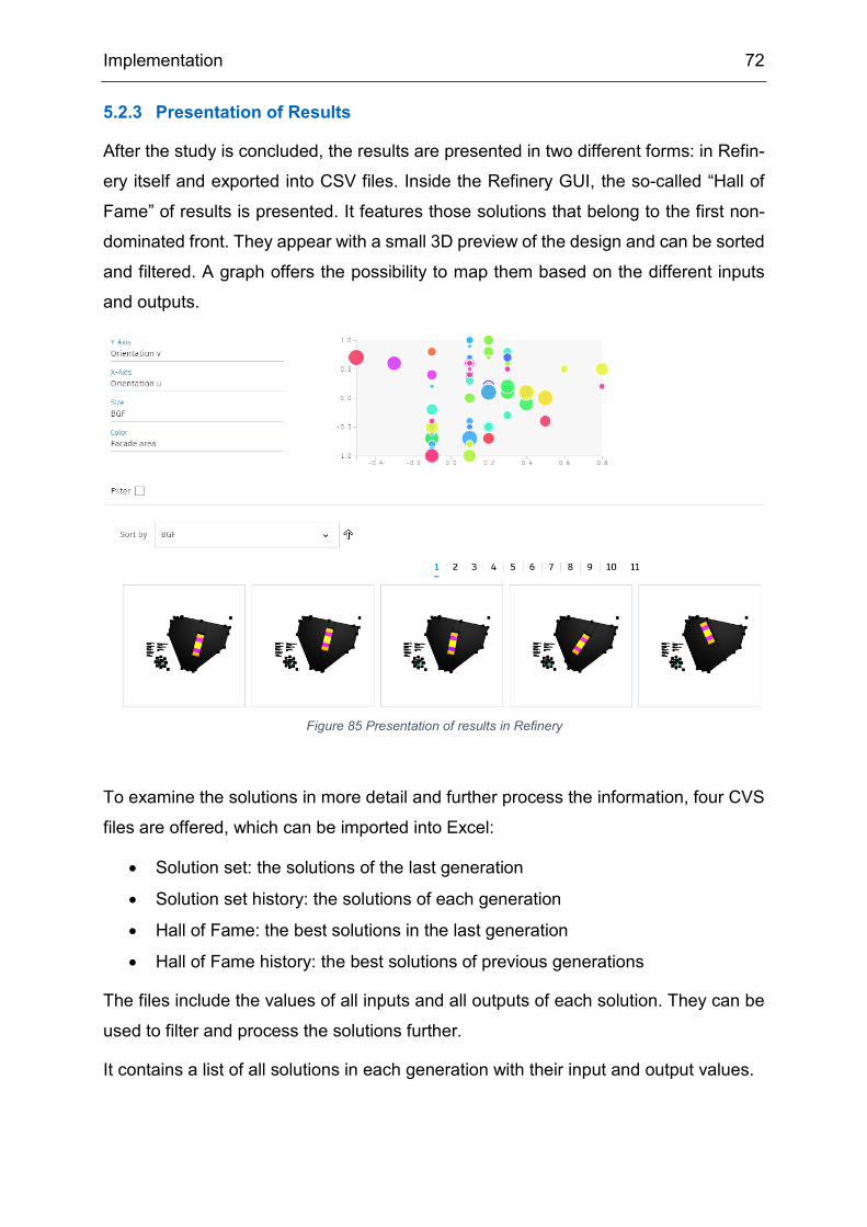
Implementation 72
5.2.3 Presentation of Results
After the study is concluded, the results are presented in two different forms: in Refin-
ery itself and exported into CSV files. Inside the Refinery GUI, the so-called “Hall of
Fame” of results is presented. It features those solutions that belong to the first non-
dominated front. They appear with a small 3D preview of the design and can be sorted
and filtered. A graph offers the possibility to map them based on the different inputs
and outputs.
To examine the solutions in more detail and further process the information, four CVS
files are offered, which can be imported into Excel:
• Solution set: the solutions of the last generation
• Solution set history: the solutions of each generation
• Hall of Fame: the best solutions in the last generation
• Hall of Fame history: the best solutions of previous generations
The files include the values of all inputs and all outputs of each solution. They can be
used to filter and process the solutions further.
It contains a list of all solutions in each generation with their input and output values.
Figure 85 Presentation of results in Refinery
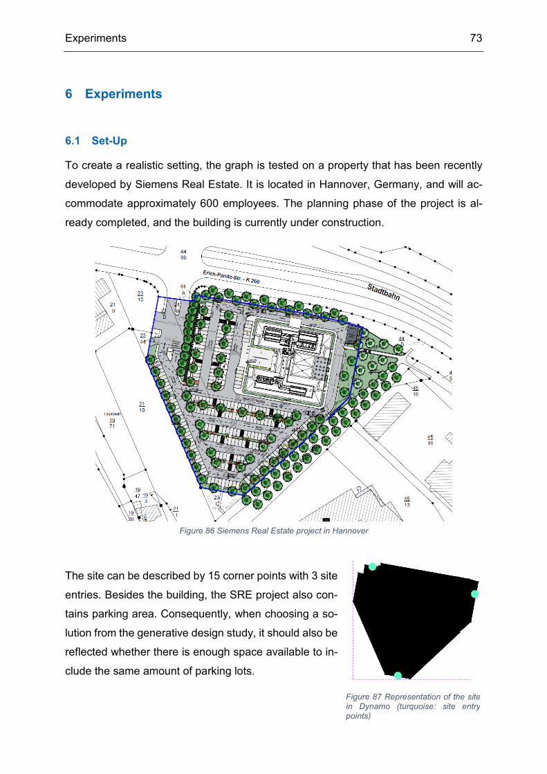
Experiments 73
6.1 Set-Up
To create a realistic setting, the graph is tested on a property that has been recently
developed by Siemens Real Estate. It is located in Hannover, Germany, and will ac-
commodate approximately 600 employees. The planning phase of the project is al-
ready completed, and the building is currently under construction.
The site can be described by 15 corner points with 3 site
entries. Besides the building, the SRE project also con-
tains parking area. Consequently, when choosing a so-
lution from the generative design study, it should also be
reflected whether there is enough space available to in-
clude the same amount of parking lots.
6 Experiments
Figure 86 Siemens Real Estate project in Hannover
Figure 87 Representation of the site in Dynamo (turquoise: site entry points)
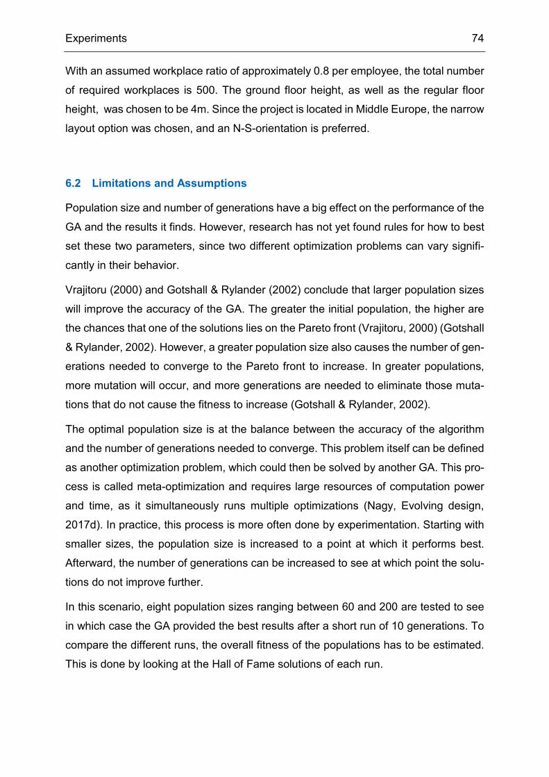
Experiments 74
With an assumed workplace ratio of approximately 0.8 per employee, the total number
of required workplaces is 500. The ground floor height, as well as the regular floor
height, was chosen to be 4m. Since the project is located in Middle Europe, the narrow
layout option was chosen, and an N-S-orientation is preferred.
6.2 Limitations and Assumptions
Population size and number of generations have a big effect on the performance of the
GA and the results it finds. However, research has not yet found rules for how to best
set these two parameters, since two different optimization problems can vary signifi-
cantly in their behavior.
Vrajitoru (2000) and Gotshall & Rylander (2002) conclude that larger population sizes
will improve the accuracy of the GA. The greater the initial population, the higher are
the chances that one of the solutions lies on the Pareto front (Vrajitoru, 2000) (Gotshall
& Rylander, 2002). However, a greater population size also causes the number of gen-
erations needed to converge to the Pareto front to increase. In greater populations,
more mutation will occur, and more generations are needed to eliminate those muta-
tions that do not cause the fitness to increase (Gotshall & Rylander, 2002).
The optimal population size is at the balance between the accuracy of the algorithm
and the number of generations needed to converge. This problem itself can be defined
as another optimization problem, which could then be solved by another GA. This pro-
cess is called meta-optimization and requires large resources of computation power
and time, as it simultaneously runs multiple optimizations (Nagy, Evolving design,
2017d). In practice, this process is more often done by experimentation. Starting with
smaller sizes, the population size is increased to a point at which it performs best.
Afterward, the number of generations can be increased to see at which point the solu-
tions do not improve further.
In this scenario, eight population sizes ranging between 60 and 200 are tested to see
in which case the GA provided the best results after a short run of 10 generations. To
compare the different runs, the overall fitness of the populations has to be estimated.
This is done by looking at the Hall of Fame solutions of each run.
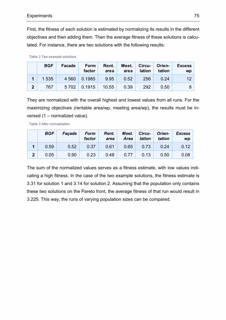
Experiments 75
First, the fitness of each solution is estimated by normalizing its results in the different
objectives and then adding them. Then the average fitness of these solutions is calcu-
lated. For instance, there are two solutions with the following results:
They are normalized with the overall highest and lowest values from all runs. For the
maximizing objectives (rentable area/wp, meeting area/wp), the results must be in-
versed (1 – normalized value).
The sum of the normalized values serves as a fitness estimate, with low values indi-
cating a high fitness. In the case of the two example solutions, the fitness estimate is
3.31 for solution 1 and 3.14 for solution 2. Assuming that the population only contains
these two solutions on the Pareto front, the average fitness of that run would result in
3.225. This way, the runs of varying population sizes can be compared.
BGF Facade Form factor
Rent. area
Meet. area
Circu-lation
Orien-tation
Excess wp
1 1 535 4 560 0.1985 9.95 0.52 256 0.24 12
2 767 5 702 0.1915 10.55 0.39 292 0.50 8
BGF Façade Form factor
Rent. area
Meet. Area
Circu-lation
Orien-tation
Excess wp
1 0.59 0.52 0.37 0.61 0.65 0.73 0.24 0.12
2 0.05 0.90 0.23 0.48 0.77 0.13 0.50 0.08
Table 2 Two example solutions
Table 3 After normalization
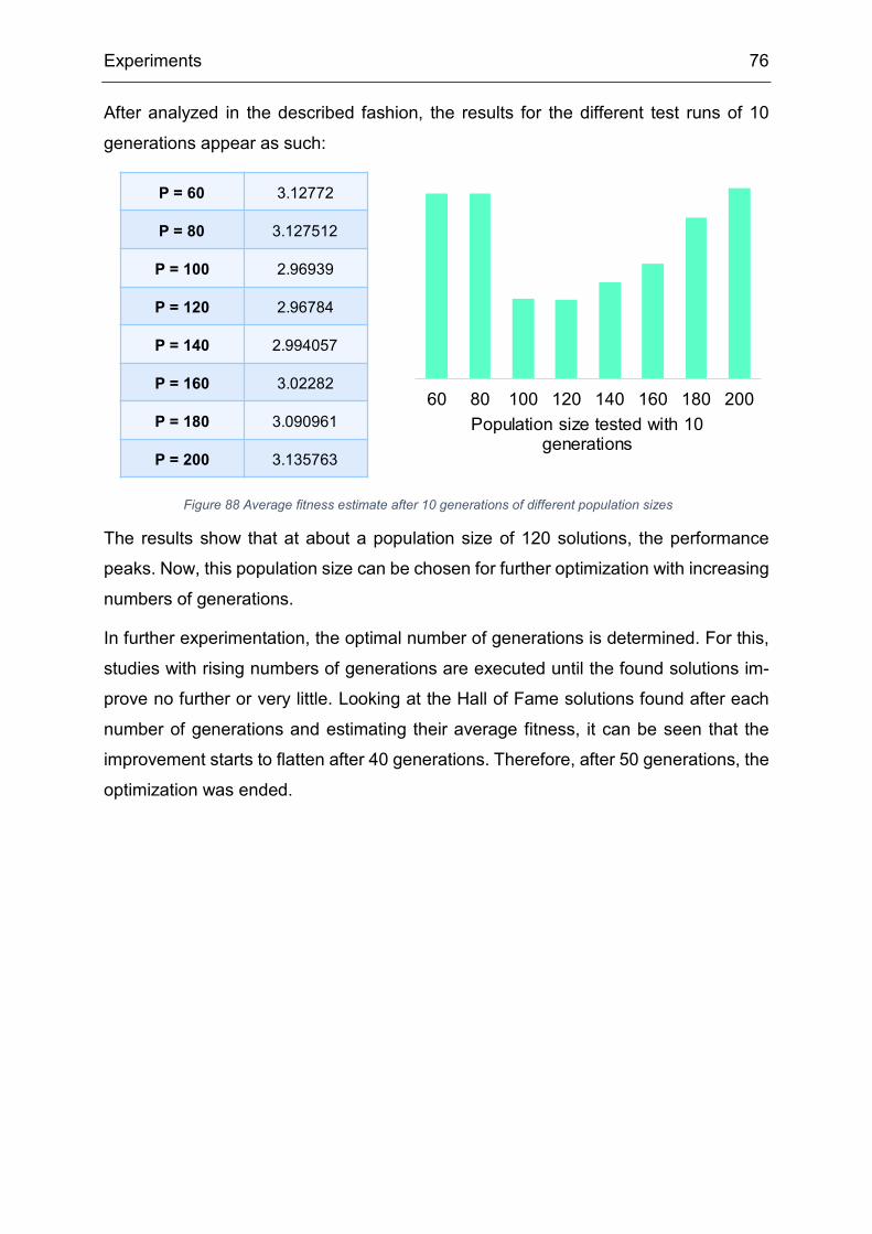
Experiments 76
After analyzed in the described fashion, the results for the different test runs of 10
generations appear as such:
The results show that at about a population size of 120 solutions, the performance
peaks. Now, this population size can be chosen for further optimization with increasing
numbers of generations.
In further experimentation, the optimal number of generations is determined. For this,
studies with rising numbers of generations are executed until the found solutions im-
prove no further or very little. Looking at the Hall of Fame solutions found after each
number of generations and estimating their average fitness, it can be seen that the
improvement starts to flatten after 40 generations. Therefore, after 50 generations, the
optimization was ended.
Figure 88 Average fitness estimate after 10 generations of different population sizes
60 80 100 120 140 160 180 200Population size tested with 10
generations
P = 60 3.12772
P = 80 3.127512
P = 100 2.96939
P = 120 2.96784
P = 140 2.994057
P = 160 3.02282
P = 180 3.090961
P = 200 3.135763

Experiments 77
As Refinery runs locally, its performance can be influenced by the power of the ma-
chine it is used on. In that case, time might also play a role in setting the population
size and number of generations. If the optimization time needs to be reduced, it is
recommended to reduce the number of generations rather than diminishing the popu-
lation size. Research has shown that larger populations tend to improve the effective-
ness more than a high number of generations (Vrajitoru, 2000).
2.52.62.72.82.9
33.13.23.33.4
1 3 5 7 9 11 13 15 17 19 21 23 25 27 29 31 33 35 37 39 41 43 45 47 49
Figure 89 Average fitness estimate after increasing numbers of generations

Experiments 78
6.3 Results
After 50 generations and with a population size of 120 solutions, the algorithm presents
14 design options that lie on the Pareto front 3 (for details, see Appendix A).
Contrary to the chosen design in Hannover, the GA favors a position on the left side of
the property. It seems to be ideal as it allows for an N-S-orientation as well as short
paths to the entrance of the building.
3 After the removal of duplicates
Figure 90 Results found in the optimization; for details see Appendix A
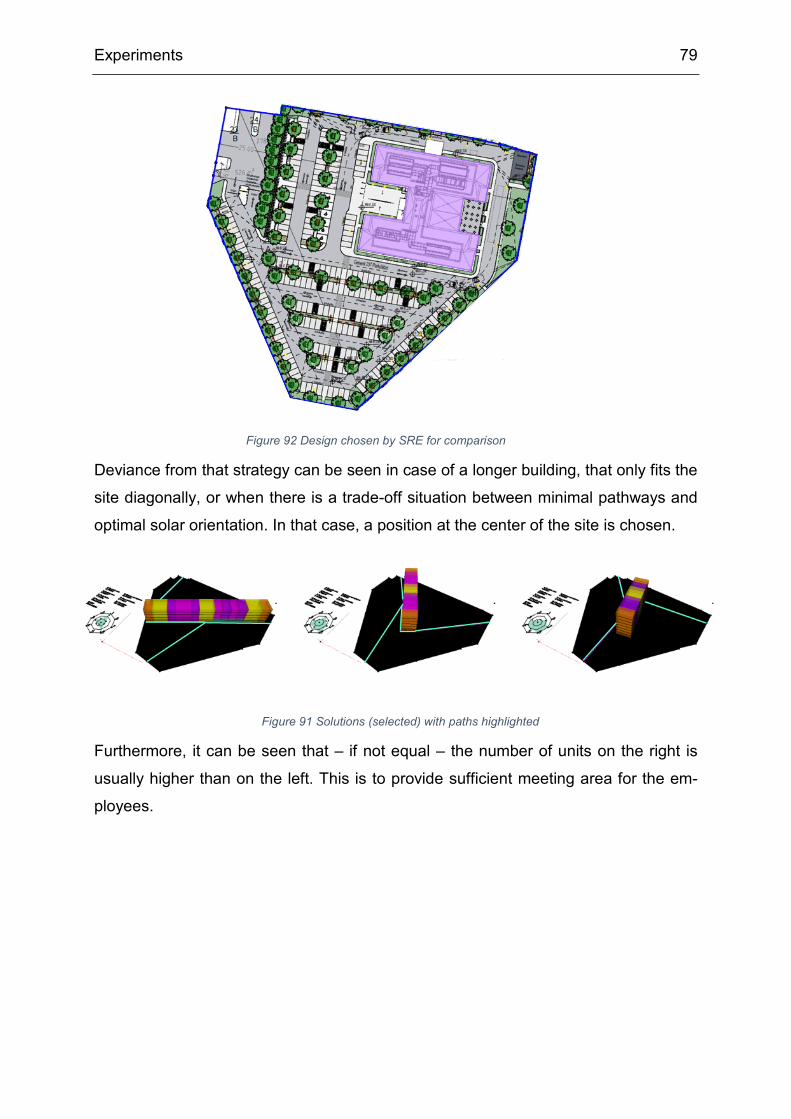
Experiments 79
Deviance from that strategy can be seen in case of a longer building, that only fits the
site diagonally, or when there is a trade-off situation between minimal pathways and
optimal solar orientation. In that case, a position at the center of the site is chosen.
Furthermore, it can be seen that – if not equal – the number of units on the right is
usually higher than on the left. This is to provide sufficient meeting area for the em-
ployees.
Figure 92 Design chosen by SRE for comparison
Figure 91 Solutions (selected) with paths highlighted
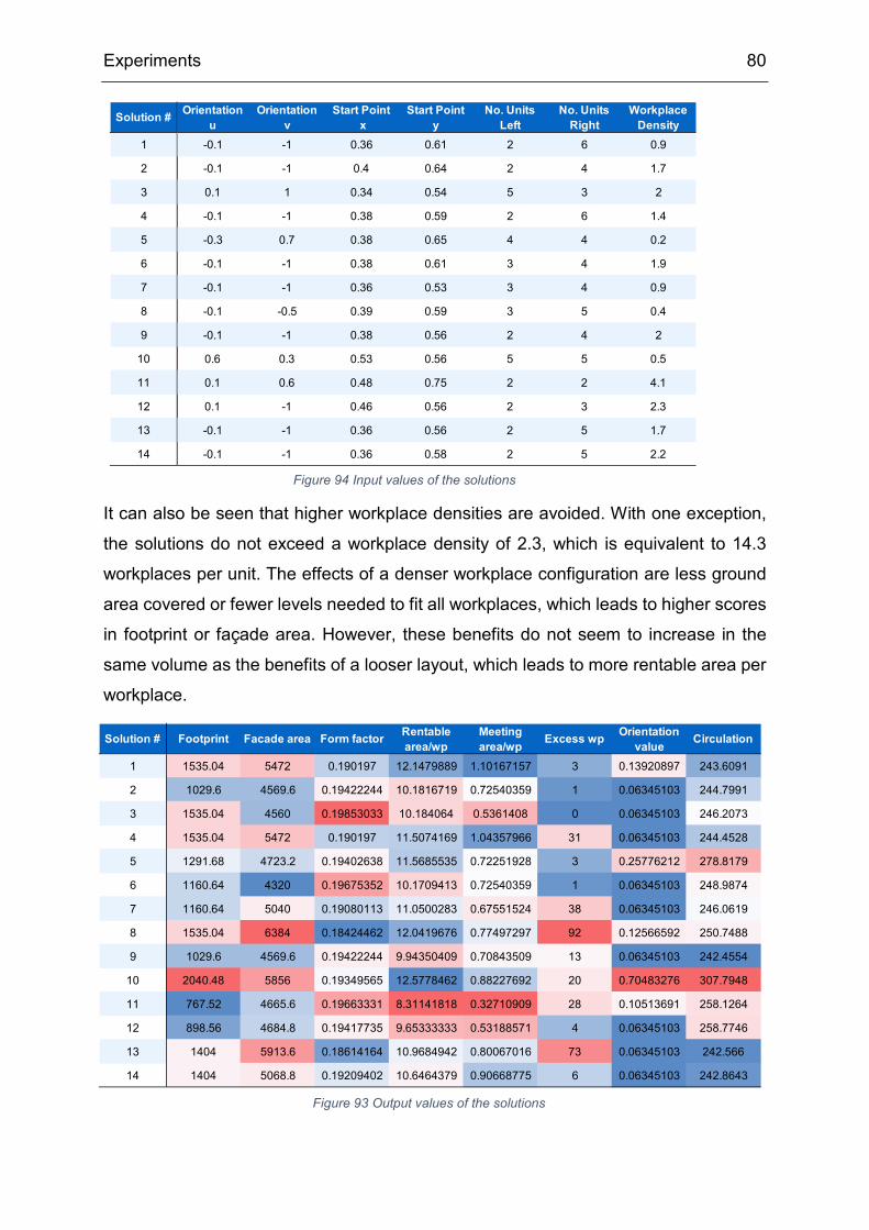
Experiments 80
It can also be seen that higher workplace densities are avoided. With one exception,
the solutions do not exceed a workplace density of 2.3, which is equivalent to 14.3
workplaces per unit. The effects of a denser workplace configuration are less ground
area covered or fewer levels needed to fit all workplaces, which leads to higher scores
in footprint or façade area. However, these benefits do not seem to increase in the
same volume as the benefits of a looser layout, which leads to more rentable area per
workplace.
Figure 94 Input values of the solutions
Figure 93 Output values of the solutions
Solution # Footprint Facade area Form factor Rentable area/wp
Meeting area/wp Excess wp Orientation
value Circulation
1 1535.04 5472 0.190197 12.1479889 1.10167157 3 0.13920897 243.6091
2 1029.6 4569.6 0.19422244 10.1816719 0.72540359 1 0.06345103 244.7991
3 1535.04 4560 0.19853033 10.184064 0.5361408 0 0.06345103 246.2073
4 1535.04 5472 0.190197 11.5074169 1.04357966 31 0.06345103 244.4528
5 1291.68 4723.2 0.19402638 11.5685535 0.72251928 3 0.25776212 278.8179
6 1160.64 4320 0.19675352 10.1709413 0.72540359 1 0.06345103 248.9874
7 1160.64 5040 0.19080113 11.0500283 0.67551524 38 0.06345103 246.0619
8 1535.04 6384 0.18424462 12.0419676 0.77497297 92 0.12566592 250.7488
9 1029.6 4569.6 0.19422244 9.94350409 0.70843509 13 0.06345103 242.4554
10 2040.48 5856 0.19349565 12.5778462 0.88227692 20 0.70483276 307.7948
11 767.52 4665.6 0.19663331 8.31141818 0.32710909 28 0.10513691 258.1264
12 898.56 4684.8 0.19417735 9.65333333 0.53188571 4 0.06345103 258.7746
13 1404 5913.6 0.18614164 10.9684942 0.80067016 73 0.06345103 242.566
14 1404 5068.8 0.19209402 10.6464379 0.90668775 6 0.06345103 242.8643
Solution #
1
2
3
4
5
6
7
8
9
10
11
12
13
14
Orientation u
Orientation v
Start Point x
Start Point y
No. Units Left
No. Units Right
Workplace Density
-0.1 -1 0.36 0.61 2 6 0.9
-0.1 -1 0.4 0.64 2 4 1.7
0.1 1 0.34 0.54 5 3 2
-0.1 -1 0.38 0.59 2 6 1.4
-0.3 0.7 0.38 0.65 4 4 0.2
-0.1 -1 0.38 0.61 3 4 1.9
-0.1 -1 0.36 0.53 3 4 0.9
-0.1 -0.5 0.39 0.59 3 5 0.4
-0.1 -1 0.38 0.56 2 4 2
0.6 0.3 0.53 0.56 5 5 0.5
0.1 0.6 0.48 0.75 2 2 4.1
0.1 -1 0.46 0.56 2 3 2.3
-0.1 -1 0.36 0.56 2 5 1.7
-0.1 -1 0.36 0.58 2 5 2.2
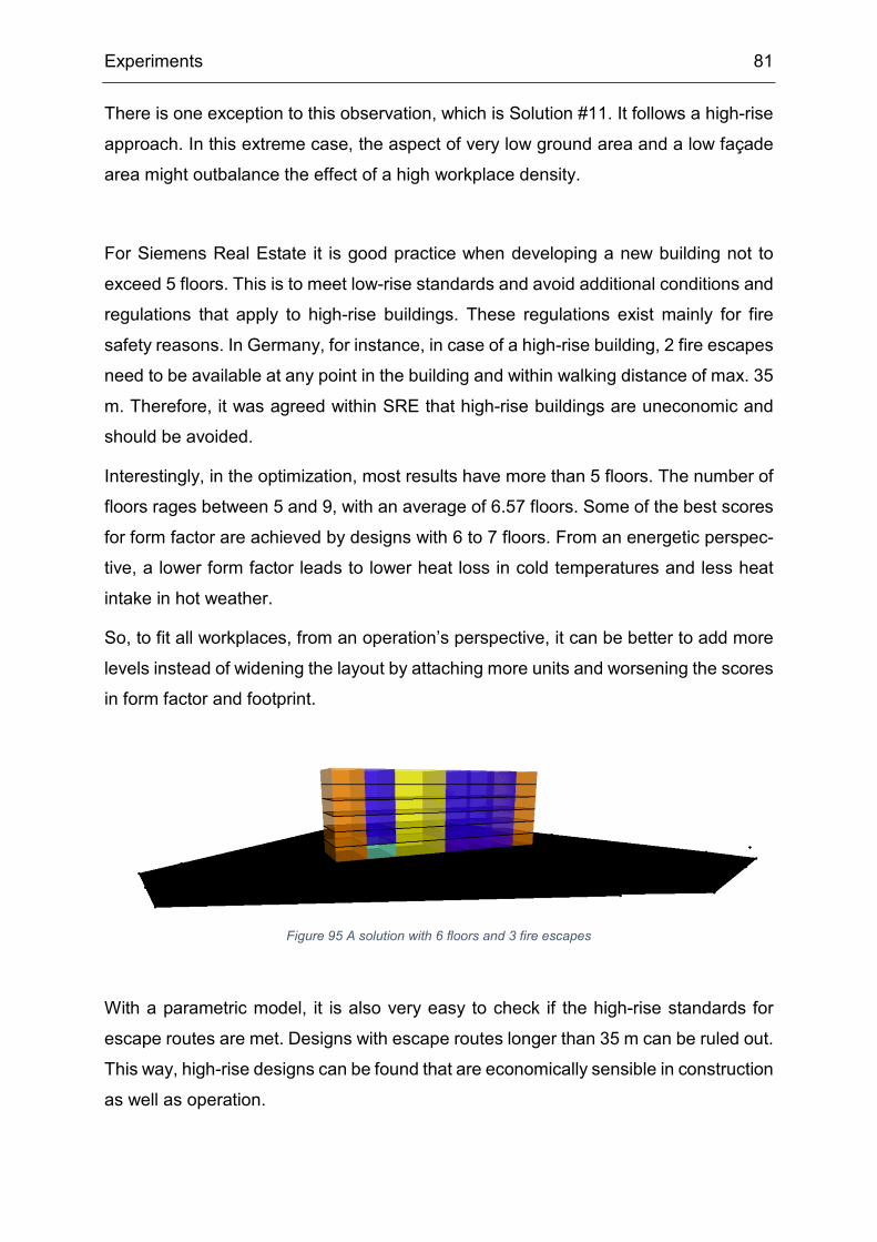
Experiments 81
There is one exception to this observation, which is Solution #11. It follows a high-rise
approach. In this extreme case, the aspect of very low ground area and a low façade
area might outbalance the effect of a high workplace density.
For Siemens Real Estate it is good practice when developing a new building not to
exceed 5 floors. This is to meet low-rise standards and avoid additional conditions and
regulations that apply to high-rise buildings. These regulations exist mainly for fire
safety reasons. In Germany, for instance, in case of a high-rise building, 2 fire escapes
need to be available at any point in the building and within walking distance of max. 35
m. Therefore, it was agreed within SRE that high-rise buildings are uneconomic and
should be avoided.
Interestingly, in the optimization, most results have more than 5 floors. The number of
floors rages between 5 and 9, with an average of 6.57 floors. Some of the best scores
for form factor are achieved by designs with 6 to 7 floors. From an energetic perspec-
tive, a lower form factor leads to lower heat loss in cold temperatures and less heat
intake in hot weather.
So, to fit all workplaces, from an operation’s perspective, it can be better to add more
levels instead of widening the layout by attaching more units and worsening the scores
in form factor and footprint.
With a parametric model, it is also very easy to check if the high-rise standards for
escape routes are met. Designs with escape routes longer than 35 m can be ruled out.
This way, high-rise designs can be found that are economically sensible in construction
as well as operation.
Figure 95 A solution with 6 floors and 3 fire escapes

Experiments 82
The 5-floor-limit might serve as an example of a rule that makes sense in traditional
design but becomes obsolete in the face of optimization. It is a rule of thumb that was
put in place to avoid high-rise regulations. However, sometimes, high-rise regulations
might be met without creating higher costs. So, limiting the building height to a maxi-
mum of 5 floors might unnecessarily narrow the solution space with some optima lying
outside the searchable space.
Experiments 83
6.4 Interview with Siemens
Six SRE project managers are interviewed on the findings of the experiment as well as
the generative design process in general. The results were presented to them as in
Appendix A. All answers can be found in Appendix B.
In general, the generative design is perceived well. It is viewed as a good approach to
achieve an objective and data-driven basis for decision making. The interviewees like
that advantages and disadvantages of different design/layout options are presented
and think it will prevent manipulation of the decision process by personal, internal, or
political interests. In comparison to a human, the computer is able to look at a much
higher number of designs. However, one interviewee stresses that it cannot be the
single source of truth. “The human touch, emotional evaluation, and inclusion of non-
tangible soft facts” still need to play a role in the evaluation. But the advantage of gen-
erative design would be that potential options would not be ruled out by “the human
nature of pre-selection and early limitation of ideas.” One interviewee states that he
“would expect this to lead to better-designed buildings as we get better at defining and
quantifying soft facts to define ‘a good indoor / outdoor environment.’”
Most interviewees agree that generative design would be beneficial for SRE. Their
standardized buildings and office modules form “a perfect basis” for generative design,
once the other configurations are implemented and rules are refined. It is seen as an
additional base for discussion and decision making and “can lead to being more effi-
cient, effective, and faster.”
One interviewee, however, has a more pessimistic view on the implementation of gen-
erative design in SRE. New processes would need to be implemented, and the educa-
tion, tools are resources are not available. Also, the parameters would need to be re-
adjusted for each project, which is seen as a hurdle.
Another point of criticism is that the set of evaluation parameters is incomprehensive
and seems arbitrary. There is a wish to include objectives like site topology, local code
requirements, and surrounding landscape and buildings.
The size of the solution set, however, is perceived as pleasant. They enjoy the possi-
bility of choice and agree the last decision should always be made by humans. The
generative design process provides a solid base upon which soft criteria can lead to a
preferred option. One suggests “it would be better to review – say max. 10 – solutions,
pick three and then run an optimization process – possibly with altered parameters or

Experiments 84
an altered weigh of the parameters. This way, people and computer could complement
each other in this iterative process”.
The Hannover experiment shows “what possibilities algorithms can offer in the early
project phase.” However, it is hard to compare the solutions to the actual design in
Hannover. One interviewee explains: “The chosen design was an H formed building.
A direct comparison would be quite difficult also because not all ConEx specification
were followed. I cannot say why but I assume there were good reasons for the deci-
sion”.
Discussion and Outlook 85
Having a clear concept of the constraints, variables, and design measures is crucial to
the success of a generative design study. In case of standardized buildings like the
Siemens Real Estate Construction Excellence, this concept already exists and only
needs to be broken down into parameters which is particularly adjuvant to a generative
design study.
When this kind of concept does not exist, it lies in the hands of the architect to be able
to abstract his vision into a set of variables and constraints, as well as carefully select
a set of objectives.
It is crucial to the outcome of the study to know exactly what objectives the design
should be optimized to. There is a virtually limitless amount of measures that a design
can be evaluated by – functional, energetic, sustainable, financial. Some might even
not be possible to asses, such as beauty or emotional stimulus. But knowing which
ones are most important to the stakeholders is key. In case of Siemens Real Estate,
there has been a well-defined process in place for how designs coming from different
architects are compared which this study could build on. But other institutions might
have to evaluate and analyze their workflows before being able to use generative de-
sign for their purposes.
Furthermore, some aspects of the design evaluation might seem trivial to the human
designer but are hard to translate into calculatable scores. For example, it is easy for
a human to solve geometric operations like placing a rectangle inside another shape if
both shapes are visually available. However, since a computer lacks this form of per-
ception, it proved difficult to implement this capacity into the system. A lot of focus was
spent on teaching the algorithm how to produce designs that lie within the site as illus-
trated in Chapter 5.2. Other aspects like beauty are even harder to implement as they
are highly subjective and hard to translate into abstract rules.
Personally, the effect of the computer taking over part of one’s work was perceived as
liberating by the researcher. Setting up the parametric model allowed for creativity,
combined with the certainty that the best versions of the parametric model would then
be found by the algorithm shifted focus on the former. In a real-life scenario, with less
7 Discussion and Outlook
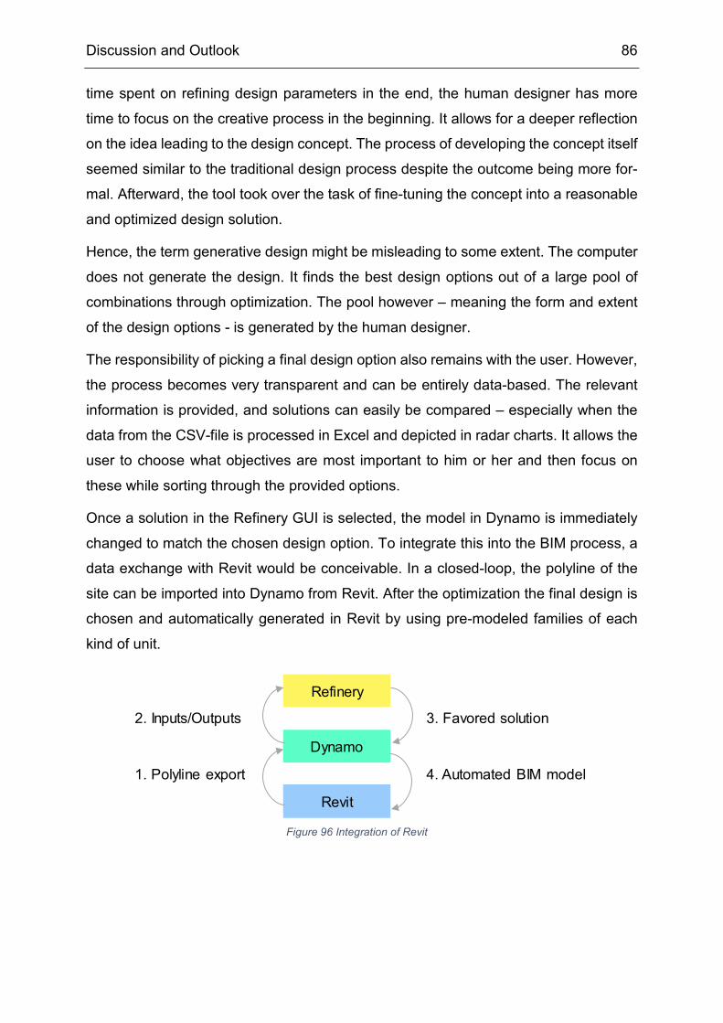
Discussion and Outlook 86
time spent on refining design parameters in the end, the human designer has more
time to focus on the creative process in the beginning. It allows for a deeper reflection
on the idea leading to the design concept. The process of developing the concept itself
seemed similar to the traditional design process despite the outcome being more for-
mal. Afterward, the tool took over the task of fine-tuning the concept into a reasonable
and optimized design solution.
Hence, the term generative design might be misleading to some extent. The computer
does not generate the design. It finds the best design options out of a large pool of
combinations through optimization. The pool however – meaning the form and extent
of the design options - is generated by the human designer.
The responsibility of picking a final design option also remains with the user. However,
the process becomes very transparent and can be entirely data-based. The relevant
information is provided, and solutions can easily be compared – especially when the
data from the CSV-file is processed in Excel and depicted in radar charts. It allows the
user to choose what objectives are most important to him or her and then focus on
these while sorting through the provided options.
Once a solution in the Refinery GUI is selected, the model in Dynamo is immediately
changed to match the chosen design option. To integrate this into the BIM process, a
data exchange with Revit would be conceivable. In a closed-loop, the polyline of the
site can be imported into Dynamo from Revit. After the optimization the final design is
chosen and automatically generated in Revit by using pre-modeled families of each
kind of unit.
Figure 96 Integration of Revit
Revit
Dynamo
Refinery
1. Polyline export
2. Inputs/Outputs
4. Automated BIM model
3. Favored solution

Discussion and Outlook 87
To further develop the parametric model for the purposes of Siemens Real Estate,
more building configurations like H-shape, L-shape, etc. could be implemented along
with an option for the wide layout.
Furthermore, the inclusion of more objectives might make the findings more compre-
hensive. The topology of the site, as well as the area surrounding the site, also plays
a significant role in design finding. Corresponding objectives can easily be added to
the evaluation. However, this would require the existence of an adequate environmen-
tal model.
References 88
Brownlee, J. (2015). Strength Pareto Evolutionary Algorithm. (Clever Algorithms:
Nature-Inspired Programming Recipes) Retrieved from
http://www.cleveralgorithms.com/nature-inspired/evolution/spea.html
Chiandussi, G., Codegone, M., Ferrero, S., & Varesio, F. (2012). Comparison of multi-
objective optimization methodologies for engineering applications. Computers
and Mathemtics with Applications.
Construction Excellence Office EMEA „Design Principles“. (2015). Siemens AG.
Dash, S., & Subudhi, B. (2016). Development of Novel Multi-Objective Based Model
for Protein Structural Class Prediction. In Handbook of Research on
Computational Intelligence Applications in Bioinformatics (S. 91-94). IGI Global.
Deb, K., Pratap, A., Agarwal, S., & Meyarivan, T. (2002). A Fast and Elitist
Multiobjective Genetic Algorithm: NSGA II. IEEE Transactions On Evulationary
Computation, Vol. 6.
Dréo, J. (2006, May 6). Multi-objective optimization. Retrieved from Wikipedia:
https://en.wikipedia.org/wiki/Multi-
objective_optimization#/media/File:Front_pareto.svg
Garcia, S., & Trinh, C. T. (2019). Comparison of Multi-Objective Evolutionary
Algorithms to Solve the Modular Cell Design Problem for Novel Biocatalysis.
MDPI.
Gotshall, S. P., & Rylander, B. (2002). Optimal Population Size and the Genetic
Algorithm.
Holland, J. H. (1984). Genetic Algorithms and Adaptation. New York: Plenum Press.
Knowles, J., & Corne, D. (1999). The Pareto archived evolution strategy: a new
baseline algorithm for Pareto multiobjective optimisation. IEEE.
Krishnapriya, S., & Rahiman, K. (2016). A Survey On Non Dominated Sorting Genetic
Algorithm II And Its Applications. International Journal Of Research In Computer
Applications And Robotics.
Kunkle, D. (2005). A Summary and Comparison of MOEA Algorithms.
References

References 89
Machairas, V., Tsangarassoulis, A., & Kleo, A. (2014). Algorithms for optimization of
building design: A review. Renewable and Sustainable Energy Reviews.
Miettinen, K. (1999). Nonlinear Multiobjective Optimization. Springer Science &
Business Media. Retrieved from https://en.wikipedia.org/wiki/Multi-
objective_optimization
Miller, B. L., & Goldberg, D. E. (1995). Genetic Algorithms, Tournament Selection and
the Effects of Noise. Complex Systems.
Multi-objective optimization. (2019, August 30). (Wikipedia) Retrieved from
https://en.wikipedia.org/wiki/NSGA-II
Nagy, D. (2017, March 20). Design optimization. (Medium) Retrieved from
https://medium.com/generative-design/design-optimization-2ec2ba3b40f7
Nagy, D. (2017a, January 24). Learning from Nature. (Medium) Retrieved from
https://medium.com/generative-design/learning-from-nature-fe5b7290e3de
Nagy, D. (2017b, January 23). The problem of learning. (Medium) Retrieved from
https://medium.com/generative-design/generative-design-introduction-
64fb2db38e1
Nagy, D. (2017c, January 24). The design space. (Medium) Retrieved from
https://medium.com/generative-design/step-1-generate-6bf73fb3a004
Nagy, D. (2017d, January 26). Evolving design. (Medium) Retrieved from
https://medium.com/generative-design/evolving-design-b0941a17b759
Samuelson Hong, W.-C. (2012). Multi Objective Optimization using GA. In Principal
Concepts in Applied Evolutionary Computation : Emerging Trends (S. 145 -
147). IGI Global.
Shea, K., Aish, R., & Gourtovia, M. (2004). Towards integrated performance-driven
generative design tools. Elsevier.
Siemens. (2019, August 30). Retrieved from Siemens Real Estate:
https://new.siemens.com/global/en/company/about/businesses/real-
estate.html
Simon, J. (2017). Evolving Floorplans. Retrieved from
http://www.joelsimon.net/evo_floorplans.html
Sivanandam, S., & Deepa, S. (2008). Introduction to Genetic Algoritms. Springer.

References 90
Stasiuk, D. (2018). Design Modeling Terminology. Proving Ground.
The Dynamo Primer. (2018). (Autodesk) Retrieved from
https://primer.dynamobim.org/03_Anatomy-of-a-Dynamo-Definition/3-
1_dynamo_nodes.html
Vrajitoru, D. (2000). Large Population or Many Generations for Genetic Algorithms?
Implications in Information Retrieval.
Walmsley, K. (2019, March 26). The Space Analysis package for Dynamo and Refinery
is now available! (Through the Interface) Retrieved from
https://www.keanw.com/2019/03/the-space-analysis-package-for-dynamo-
and-refinery-is-now-available.html
Yusoff, Y., Ngadiman, M. S., & Zain, A. M. (2011). Overview of NSGA-II for Optimizing
Machining Process. Elsevier Ltd. Selection.
Zimmermann, P. D. (2017). Schlüsselfertiger Hoch- und Ingenieurbau. Lehrstuhl für
Bauprozessmanagement und Immobilienentwicklung, TU München.
References 91
Figure 1 Original floorplan of a school in Maine, USA (Simon, 2017) ......................... 7
Figure 2 Results after optimization for minimal traffic between classes (left) and additional optimization for minimal fire escape paths (right); from: Simon (2017) ..................................................................................... 8
Figure 3 Results after windows were implemented as additional fitness function. Classrooms received higher priority for daylight than storage rooms; from: Simon (2017) ............................................................................ 8
Figure 4 The evolutionary process in nature; inspired by Nagy (2017a) ................... 11
Figure 5 Iterative optimization process ..................................................................... 12
Figure 6 Three different façade configurations ......................................................... 13
Figure 7 The function of the parametric model ......................................................... 13
Figure 8 “Point C is not on the Pareto frontier because it is dominated by both point A and point B. Points A and B are not strictly dominated by any other, and hence lie on the frontier” (Dréo, 2006); inspired by Dréo (2006) ........................................................................................................ 15
Figure 9 Basic model of a genetic algorithm (GA); inspired by Nagy, 2017b ............ 16
Figure 10 When we look at A, it is not dominated by any other solution. Therefore, its domination count is 0. ..................................................................... 19
Figure 11 When we look at B, it is dominated by A and F. Therefore, its domination count is 2 and B is added to the dominated set Sp of A and F......... 19
Figure 12 After all comparisons are finished, each solution is equipped with a domination count and a set of dominated solutions......................... 20
Figure 13 Pseudocode of the fast nondominated-sorting algorithm; from: Deb et al. (2002) .............................................................................................. 20
Figure 14 In the first step, all solutions with a domination count of 0 are grouped into the first front. The members of their dominated sets Sp receive a reduction of 1 in their domination count ........................................... 21
Figure 15 In the second step, this process repeated with the solutions that now have a domination count of 0. ..................................................................... 21
Figure 16 This process is repeated until all solutions are sorted into fronts.............. 21
List of Figures

References 92
Figure 17 Crowding distance calculation (Points marked in purple are solutions of the same nondominated front); inspired by Deb et al. (2002) ................ 22
Figure 18 The crowded-comparison operator < 𝑖𝑖 .................................................... 22
Figure 19 The NSGA-II procedure; inspired by Deb et al. (2002) ............................. 23
Figure 20 Single-point crossover .............................................................................. 25
Figure 21 Uniform crossover; inspired by Sivanandam & Deepa (2008) .................. 26
Figure 22 Flipping; inspired by Sivanandam & Deepa (2008) ................................... 27
Figure 23 Interchanging; inspired by Sivanandam & Deepa (2008) ......................... 27
Figure 24 Reserving; inspired by Sivanandam & Deepa (2008) ............................... 27
Figure 25 Phases of real estate development; inspired by Zimmermann (2017) ...... 29
Figure 26 Quality levels in ConEx ............................................................................. 31
Figure 27 Core unit (yellow), office units (blue) and seam units (orange) in a standard ConEx layout ................................................................................... 31
Figure 28 The site polyline defined by corner points in form of coordinates ............. 33
Figure 29 Determination of the start point according to a virtual bounding box ....... 33
Figure 30 Different directions of the orientation vector based on u and v values ...... 34
Figure 31 Step one: The largest inscribed rectangle is created ................................ 34
Figure 32 Step two: The core is placed so that its centre lies on the start point ....... 34
Figure 33 Step three: The units are placed on either side of the core ...................... 35
Figure 34 Step four: The last unit on each side is turned into a seam unit ............... 35
Figure 35 The 6 different workplace configurations, from left: 20, 17, 15, 14, 12, 11 desks per unit .................................................................................. 36
Figure 36 Step five: Each unit is assigned with a number of workplaces ................ 36
Figure 37 Different workplace configurations on the ground floor, from left: 16, 13, 10 desks per unit .................................................................................. 37
Figure 38 Step six: Floors are replicated until total number of workplaces is reached ........................................................................................................ 37
Figure 39 Three versions of a model with different parameter values; left: workplace density set to a very low value, hence more floors have to be installed to accommodate all employees; centre: workplace density set to a very low value, some upper floors become obsolete since workplaces are more densely arranged; right: increased number of units on the right,

References 93
number of floors sinks even more, but model becomes invalid because it exceed the borders of the site ...................................................... 38
Figure 40 Explanation of orientation value................................................................ 42
Figure 41 Computation of pathways (in pink) ........................................................... 42
Figure 42 The Randomize method ........................................................................... 44
Figure 43 The Cross Product method ....................................................................... 44
Figure 44 The Like This method ............................................................................... 44
Figure 45 Example cuboid ........................................................................................ 45
Figure 46 The form factor of the cuboid according to growing values of x ................ 46
Figure 47 Dynamo graph .......................................................................................... 47
Figure 48 Dynamo node ........................................................................................... 47
Figure 49 Results after 1 generation (left), 6 generations (centre) and 10 generations (right) ............................................................................................... 48
Figure 50 Position and orientation of the cuboid ....................................................... 49
Figure 51 All possible solutions sorted by their position on x and y axis; each dot contains 4 solutions with different rotations ..................................... 50
Figure 52 Overview of the generated solutions, each line represents one solution .. 50
Figure 53 Solutions filtered by containment value and orientation value .................. 51
Figure 54 Coordinates of the selected solutions ....................................................... 51
Figure 55 Visualisation of the 5 solutions found through the brute force approach .. 51
Figure 56 Solutions found in the optimization study ................................................. 52
Figure 57 Visualisation of the 5 solutions found in the optimization study ................ 52
Figure 58 Workflow of the generative design study .................................................. 53
Figure 59 Constraints, variables and objectives of the generative design study ....... 54
Figure 60 Implementation of the parametric model .................................................. 56
Figure 61 The start point is positioned in relation to the bounding box ..................... 56
Figure 62 The width of the rectangle is created ........................................................ 57
Figure 63 The rectangle is closed ............................................................................. 57
Figure 64 Failed construction of the rectangle .......................................................... 57
Figure 65 Example of a custom Python node to calculate the corners of the core ... 58
References 94
Figure 66 Left: The corner points of the units are calculated, right: The rectangles are extruded to form the units of the ground floor .................................. 58
Figure 67 Example of the workplace distribution algorithm for a density of 3.2 ........ 59
Figure 68 The solid formed by all units is exploded into its surfaces ........................ 61
Figure 69 When the workplace density is changed to a lower value more floors are needed ............................................................................................ 62
Figure 70 Path finding in Dynamo ............................................................................ 62
Figure 71 Custom nodes from the Space Analysis package .................................... 62
Figure 72 Different versions of the model with a radar chart of their evaluation ....... 63
Figure 73 An invalid solution ..................................................................................... 64
Figure 74 The example cuboid ................................................................................. 64
Figure 75 Workflow of generating and evaluating the cuboid ................................... 64
Figure 76 The algorithm is now faced with the challenge to optimize length as well as position of the cuboid ...................................................................... 65
Figure 77 The fixed penalty method ......................................................................... 65
Figure 78 The added objective method .................................................................... 66
Figure 79 The penalty factor method ........................................................................ 66
Figure 80 Number of generations each method needed to optimize its solutions ..... 67
Figure 81 Inputs and outputs in the Dynamo user interface ..................................... 69
Figure 82 Creating a new study in Refinery .............................................................. 70
Figure 83 Objectives in the Refinery user interface .................................................. 70
Figure 84 Settings in the Refinery user interface ...................................................... 71
Figure 85 Presentation of results in Refinery ............................................................ 72
Figure 86 Siemens Real Estate project in Hannover ................................................ 73
Figure 87 Representation of the site in Dynamo (turquoise: site entry points) .......... 73
Figure 88 Average fitness estimate after 10 generations of different population sizes ........................................................................................................ 76
Figure 89 Average fitness estimate after increasing numbers of generations .......... 77
Figure 90 Results found in the optimization; for details see Appendix A .................. 78
Figure 91 Solutions (selected) with paths highlighted ............................................... 79
Figure 92 Design chosen by SRE for comparison .................................................... 79

References 95
Figure 93 Output values of the solutions .................................................................. 80
Figure 94 Input values of the solutions ..................................................................... 80
Figure 95 A solution with 6 floors and 3 fire escapes ............................................... 81
Figure 96 Integration of Revit ................................................................................... 86

References 96
Table 1 Rentable area in each kind of unit ............................................................... 39
Table 2 Two example solutions ................................................................................ 75
Table 3 After normalization ....................................................................................... 75
List of Tables

References 97
Appendix A

Ove
rvie
w o
f res
ults
Ove
rvie
w o
f res
ults
Solu
tion
#Fo
otpr
int
Faca
de a
rea
Form
fact
orR
enta
ble
area
/wp
Mee
ting
area
/wp
Exce
ss w
pO
rient
atio
n va
lue
Circ
ulat
ion
Orie
ntat
ion
uO
rient
atio
n v
Star
t Poi
nt x
Star
t Poi
nt
yN
o. U
nits
Lef
tN
o. U
nits
Rig
htW
orkp
lace
D
ensi
ty1
1535
.04
5472
0.19
0196
998
12.1
4798
887
1.10
1671
571
30.
1392
0897
524
3.60
91-0
.1-1
0.36
0.61
26
0.9
210
29.6
4569
.60.
1942
2244
410
.181
6718
60.
7254
0359
31
0.06
3451
035
244.
7991
-0.1
-10.
40.
642
41.
7
315
35.0
445
600.
1985
3033
110
.184
064
0.53
6140
80
0.06
3451
035
246.
2073
0.1
10.
340.
545
32
415
35.0
454
720.
1901
9699
811
.507
4169
51.
0435
7966
131
0.06
3451
035
244.
4528
-0.1
-10.
380.
592
61.
4
512
91.6
847
23.2
0.19
4026
384
11.5
6855
348
0.72
2519
284
30.
2577
6211
827
8.81
79-0
.30.
70.
380.
654
40.
2
611
60.6
443
200.
1967
5351
510
.170
9413
20.
7254
0359
31
0.06
3451
035
248.
9874
-0.1
-10.
380.
613
41.
9
711
60.6
450
400.
1908
0113
411
.050
0282
50.
6755
1524
238
0.06
3451
035
246.
0619
-0.1
-10.
360.
533
40.
9
815
35.0
463
840.
1842
4461
712
.041
9675
70.
7749
7297
392
0.12
5665
916
250.
7488
-0.1
-0.5
0.39
0.59
35
0.4
910
29.6
4569
.60.
1942
2244
49.
9435
0409
40.
7084
3508
813
0.06
3451
035
242.
4554
-0.1
-10.
380.
562
42
1020
40.4
858
560.
1934
9564
812
.577
8461
50.
8822
7692
320
0.70
4832
765
307.
7948
0.6
0.3
0.53
0.56
55
0.5
1176
7.52
4665
.60.
1966
3331
28.
3114
1818
20.
3271
0909
128
0.10
5136
913
258.
1264
0.1
0.6
0.48
0.75
22
4.1
1289
8.56
4684
.80.
1941
7735
9.65
3333
333
0.53
1885
714
40.
0634
5103
525
8.77
460.
1-1
0.46
0.56
23
2.3
1314
0459
13.6
0.18
6141
636
10.9
6849
424
0.80
0670
157
730.
0634
5103
524
2.56
6-0
.1-1
0.36
0.56
25
1.7
1414
0450
68.8
0.19
2094
017
10.6
4643
794
0.90
6687
747
60.
0634
5103
524
2.86
43-0
.1-1
0.36
0.58
25
2.2
For m
ore
deta
iled
info
rmat
ion
on e
ach
solu
tion
plea
se c
lick
on th
e re
spec
tive
#
1V
ery
good
resu
lt2
Goo
d re
sult
3O
k re
sult
4P
oor r
esul
t5
Ver
y po
or re
sult
Page
1

Overview of results
Solution #1
Variable Input11 Orientation u -0.112 Orientation v -113 Start Point x 0.3614 Start Point y 0.6115 No. Units Left 216 No. Units Right 617 Workplace Density 0.9
Item Result2 Footprint 1535.043 Facade area 54724 Form factor 0.1901975 Rentable area/wp 12.14798896 Meeting Area/wp 1.101671577 Excess WP 38 Orientation value 0.139208979 Circulation 243.6091
Model output
Input variables
Results radar chart
Graphical overview of result
Footprint
Facade area
Form factor
Rentablearea/wp
MeetingArea/wp
Excess WP
Orientationvalue
Circulation
Page 2

Overview of results
Solution #2
Variable Input11 Orientation u -0.112 Orientation v -113 Start Point x 0.414 Start Point y 0.6415 No. Units Left 216 No. Units Right 417 Workplace Density 1.7
Item Result2 Footprint 1029.63 Facade area 4569.64 Form factor 0.194222445 Rentable area/wp 10.18167196 Meeting Area/wp 0.725403597 Excess WP 18 Orientation value 0.063451039 Circulation 244.7991
Input variables
Model output Results radar chart
Graphical overview of result
Footprint
Facade area
Form factor
Rentablearea/wp
MeetingArea/wp
Excess WP
Orientationvalue
Circulation
Page 3

Overview of results
Solution #3
Variable Input11 Orientation u 0.112 Orientation v 113 Start Point x 0.3414 Start Point y 0.5415 No. Units Left 516 No. Units Right 317 Workplace Density 2
Item Result2 Footprint 1535.043 Facade area 45604 Form factor 0.198530335 Rentable area/wp 10.1840646 Meeting Area/wp 0.53614087 Excess WP 08 Orientation value 0.063451039 Circulation 246.2073
Input variables
Model output Results radar chart
Graphical overview of result
Footprint
Facade area
Form factor
Rentablearea/wp
MeetingArea/wp
Excess WP
Orientationvalue
Circulation
Page 4

Overview of results
Solution #4
Variable Input11 Orientation u -0.112 Orientation v -113 Start Point x 0.3814 Start Point y 0.5915 No. Units Left 216 No. Units Right 617 Workplace Density 1.4
Item Result2 Footprint 1535.043 Facade area 54724 Form factor 0.1901975 Rentable area/wp 11.50741696 Meeting Area/wp 1.043579667 Excess WP 318 Orientation value 0.063451039 Circulation 244.4528
Input variables
Model output Results radar chart
Graphical overview of result
Footprint
Facade area
Form factor
Rentablearea/wp
MeetingArea/wp
Excess WP
Orientationvalue
Circulation
Page 5
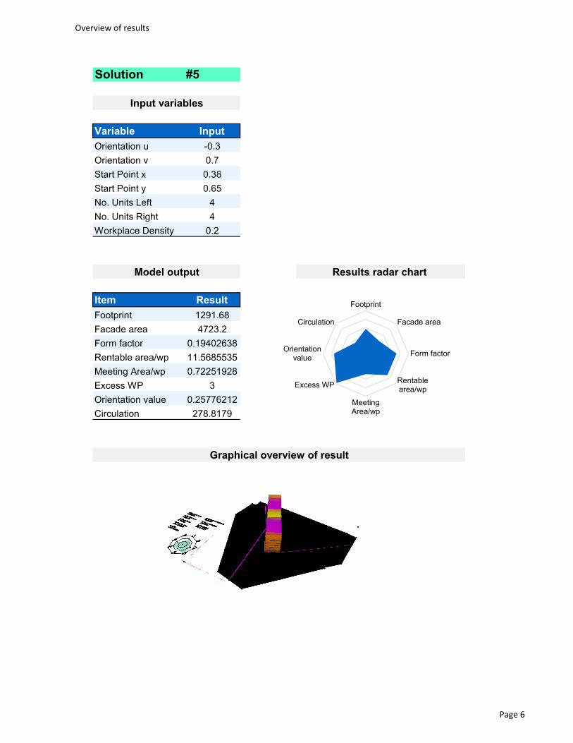
Overview of results
Solution #5
Variable Input11 Orientation u -0.312 Orientation v 0.713 Start Point x 0.3814 Start Point y 0.6515 No. Units Left 416 No. Units Right 417 Workplace Density 0.2
Item Result2 Footprint 1291.683 Facade area 4723.24 Form factor 0.194026385 Rentable area/wp 11.56855356 Meeting Area/wp 0.722519287 Excess WP 38 Orientation value 0.257762129 Circulation 278.8179
Input variables
Model output Results radar chart
Graphical overview of result
Footprint
Facade area
Form factor
Rentablearea/wp
MeetingArea/wp
Excess WP
Orientationvalue
Circulation
Page 6

Overview of results
Solution #6
Variable Input11 Orientation u -0.112 Orientation v -113 Start Point x 0.3814 Start Point y 0.6115 No. Units Left 316 No. Units Right 417 Workplace Density 1.9
Item Result2 Footprint 1160.643 Facade area 43204 Form factor 0.196753525 Rentable area/wp 10.17094136 Meeting Area/wp 0.725403597 Excess WP 18 Orientation value 0.063451039 Circulation 248.9874
Input variables
Model output Results radar chart
Graphical overview of result
Footprint
Facade area
Form factor
Rentablearea/wp
MeetingArea/wp
Excess WP
Orientationvalue
Circulation
Page 7

Overview of results
Solution #7
Variable Input11 Orientation u -0.112 Orientation v -113 Start Point x 0.3614 Start Point y 0.5315 No. Units Left 316 No. Units Right 417 Workplace Density 0.9
Item Result2 Footprint 1160.643 Facade area 50404 Form factor 0.190801135 Rentable area/wp 11.05002836 Meeting Area/wp 0.675515247 Excess WP 388 Orientation value 0.063451039 Circulation 246.0619
Input variables
Model output Results radar chart
Graphical overview of result
Footprint
Facade area
Form factor
Rentablearea/wp
MeetingArea/wp
Excess WP
Orientationvalue
Circulation
Page 8
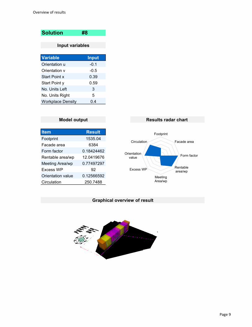
Overview of results
Solution #8
Variable Input11 Orientation u -0.112 Orientation v -0.513 Start Point x 0.3914 Start Point y 0.5915 No. Units Left 316 No. Units Right 517 Workplace Density 0.4
Item Result2 Footprint 1535.043 Facade area 63844 Form factor 0.184244625 Rentable area/wp 12.04196766 Meeting Area/wp 0.774972977 Excess WP 928 Orientation value 0.125665929 Circulation 250.7488
Input variables
Model output Results radar chart
Graphical overview of result
Footprint
Facade area
Form factor
Rentablearea/wp
MeetingArea/wp
Excess WP
Orientationvalue
Circulation
Page 9

Overview of results
Solution #9
Variable Input11 Orientation u -0.112 Orientation v -113 Start Point x 0.3814 Start Point y 0.5615 No. Units Left 216 No. Units Right 417 Workplace Density 2
Item Result2 Footprint 1029.63 Facade area 4569.64 Form factor 0.194222445 Rentable area/wp 9.943504096 Meeting Area/wp 0.708435097 Excess WP 138 Orientation value 0.063451039 Circulation 242.4554
Input variables
Model output Results radar chart
Graphical overview of result
Footprint
Facade area
Form factor
Rentablearea/wp
MeetingArea/wp
Excess WP
Orientationvalue
Circulation
Page 10
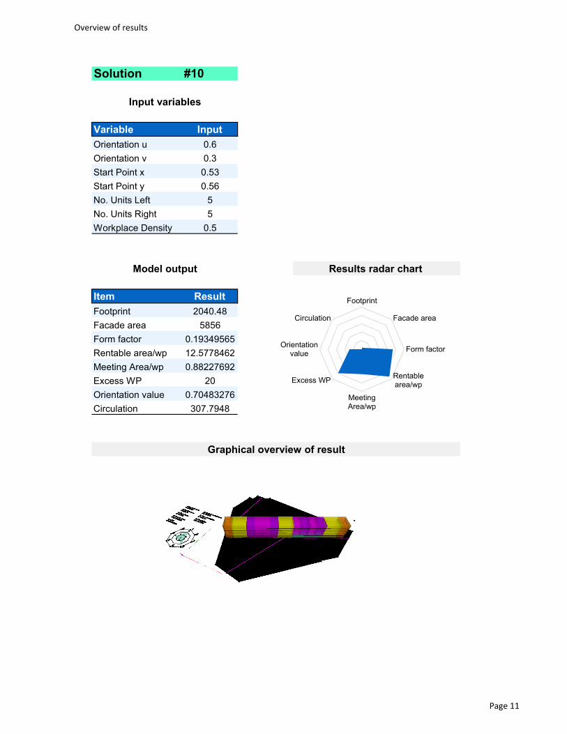
Overview of results
Solution #10
Variable Input11 Orientation u 0.612 Orientation v 0.313 Start Point x 0.5314 Start Point y 0.5615 No. Units Left 516 No. Units Right 517 Workplace Density 0.5
Item Result2 Footprint 2040.483 Facade area 58564 Form factor 0.193495655 Rentable area/wp 12.57784626 Meeting Area/wp 0.882276927 Excess WP 208 Orientation value 0.704832769 Circulation 307.7948
Input variables
Model output Results radar chart
Graphical overview of result
Footprint
Facade area
Form factor
Rentablearea/wp
MeetingArea/wp
Excess WP
Orientationvalue
Circulation
Page 11
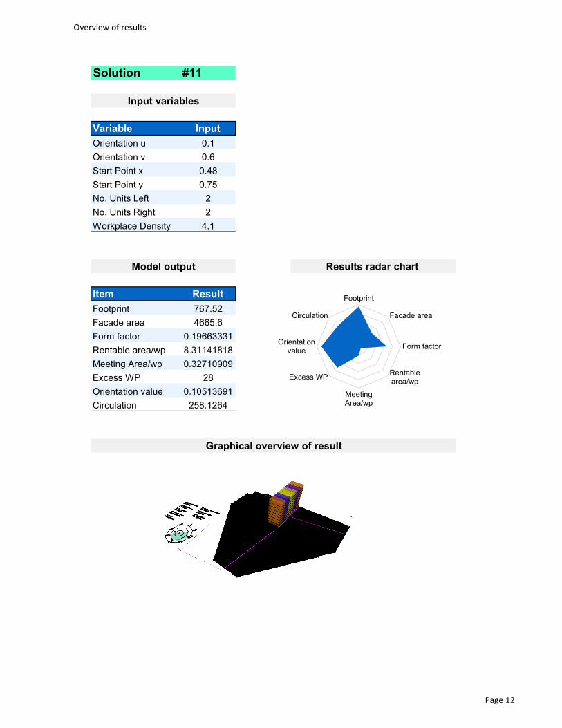
Overview of results
Solution #11
Variable Input11 Orientation u 0.112 Orientation v 0.613 Start Point x 0.4814 Start Point y 0.7515 No. Units Left 216 No. Units Right 217 Workplace Density 4.1
Item Result2 Footprint 767.523 Facade area 4665.64 Form factor 0.196633315 Rentable area/wp 8.311418186 Meeting Area/wp 0.327109097 Excess WP 288 Orientation value 0.105136919 Circulation 258.1264
Input variables
Model output Results radar chart
Graphical overview of result
Footprint
Facade area
Form factor
Rentablearea/wp
MeetingArea/wp
Excess WP
Orientationvalue
Circulation
Page 12
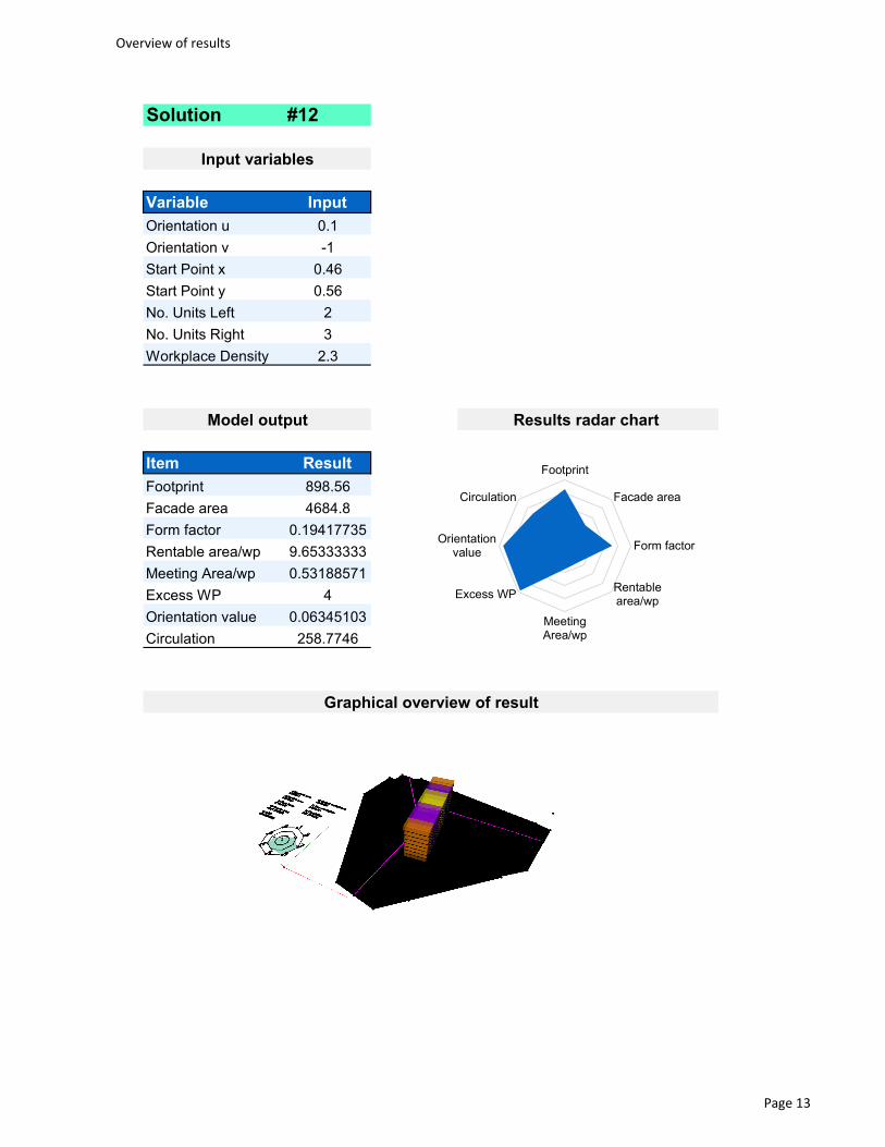
Overview of results
Solution #12
Variable Input11 Orientation u 0.112 Orientation v -113 Start Point x 0.4614 Start Point y 0.5615 No. Units Left 216 No. Units Right 317 Workplace Density 2.3
Item Result2 Footprint 898.563 Facade area 4684.84 Form factor 0.194177355 Rentable area/wp 9.653333336 Meeting Area/wp 0.531885717 Excess WP 48 Orientation value 0.063451039 Circulation 258.7746
Input variables
Model output Results radar chart
Graphical overview of result
Footprint
Facade area
Form factor
Rentablearea/wp
MeetingArea/wp
Excess WP
Orientationvalue
Circulation
Page 13
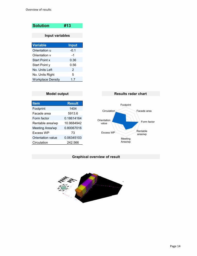
Overview of results
Solution #13
Variable Input11 Orientation u -0.112 Orientation v -113 Start Point x 0.3614 Start Point y 0.5615 No. Units Left 216 No. Units Right 517 Workplace Density 1.7
Item Result2 Footprint 14043 Facade area 5913.64 Form factor 0.186141645 Rentable area/wp 10.96849426 Meeting Area/wp 0.800670167 Excess WP 738 Orientation value 0.063451039 Circulation 242.566
Input variables
Model output Results radar chart
Graphical overview of result
Footprint
Facade area
Form factor
Rentablearea/wp
MeetingArea/wp
Excess WP
Orientationvalue
Circulation
Page 14
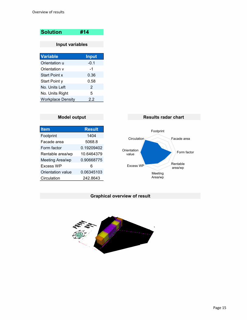
Overview of results
Solution #14
Variable Input11 Orientation u -0.112 Orientation v -113 Start Point x 0.3614 Start Point y 0.5815 No. Units Left 216 No. Units Right 517 Workplace Density 2.2
Item Result2 Footprint 14043 Facade area 5068.84 Form factor 0.192094025 Rentable area/wp 10.64643796 Meeting Area/wp 0.906687757 Excess WP 68 Orientation value 0.063451039 Circulation 242.8643
Input variables
Model output Results radar chart
Graphical overview of result
Footprint
Facade area
Form factor
Rentablearea/wp
MeetingArea/wp
Excess WP
Orientationvalue
Circulation
Page 15
References 98
What are your thoughts on the generative design approach overall?
Interviewee A
It’s a very good approach to show up an objective and data driven basis for decision
making. Presented pros and cons of different building design/layout possibilities - i.e.
decision processes are often kind of “manipulated” by personal, internal, political, stra-
tegic or other stakeholder interests, with sometimes significant consequences in plan-
ning and execution phase or even in the end for the customer during/after handover.
This approach supports transparent and objective prioritizing of design criteria and
data bases decision making.
Needless to say all the positive commercial aspects like cost calculation, rating of de-
sign/concept changes, etc..
Interviewee B
Ein guter Ansatz für die Optimierung von Gebäuden in der frühen Phase. In Kombina-
tion mit dem Wissen über die örtlichen und baurechtlichen Gegebenheiten ist das in
Zukunft eine gute Unterstützung zur Bestimmung des optimalen Designs. Mir fehlen
jedoch die Parameter, die sich aus den Gegebenheiten des Grundstücks ergeben
(z.B.: Zufahrt, Höhenverlauf).
Interviewee C
In my opinion generative design generally offers an enormous potential in the field of
architecture – especially in the early project phases. Wherever design plays a role,
generative design and artificial intelligence can help due to the very high number of
design variants. For example, in other industries generic design is almost standard.
For example, in the automotive or food industries. I think the example of the Hannover
building already shows SRE, what possibilities algorithms can offer in the early project
phase. An automatic configuration tool for office buildings, based on ConEx, could be
a first step for SRE. But it can’t be the single source of truth.
Appendix B
References 99
Interviewee D
The future for (building) design is via parametric design, as I see it. The opportunity to
connect design parameters and letting them interact via modelling will bring new in-
sights into the prioritizing of technical parameters and quantifiable soft facts. Will it fix
all? No. The “human touch”, emotional evaluation and inclusion of non-tangible soft
facts will still need to be added as part of an evaluation of the machine generated out
option. The upside, as I see it, is that the human nature of pre-selection or early limita-
tion of ideas is not limiting theoretical options up front. I would expect this to lead to
better designed buildings as we get better at defining and quantifying soft facts to de-
fine “a good indoor / outdoor environment”.
Interviewee E
In general, it is an interesting approach to finding optimal design alternatives. It is,
however, very limited with the typical constraints that we are facing in the conceptual
phase. Most decision in the end are arbitrary and based on aesthetics and the sur-
rounding landscape or how the landscape will be altered to make a comfortable envi-
ronment.
Interviewee F
A suitable approach for very early design phases and for evaluations regarding the
possibilities of suing a site. Local code requirements 8for example: if a building has to
stand on a certain line, not “somehow” on the site, should be possible to enter, to en-
sure that the options generated are actually – at least somewhat – realistic.
It would also be helpful if the parameters can be changes – this is what happens in an
iterative design process: not only the solutions develop, but also the parameters they
are measured against, because we never know everything from the beginning.

References 100
Do you think that it can be beneficial to Siemens Real Estate in the near future?
Interviewee A
Yes! Standardized building configurations and office modules are a perfect basis for
this approach.
Interviewee B
Ja. Für die Entwicklung zukünftiger Design ist das eine gute Unterstützung und bietet
einen zusätzlichen Diskussions- und Entscheidungsansatz.
Interviewee C Yes, it may be beneficial for SRE to use an iterative generic design process in the near
future. Generative design can help SRE to find the most efficient form in the early
project phase. If SRE has such an automatic configuration tool, SRE could consider a
wide range of solutions for customers. This can lead to being more efficient, effective
and faster. With generic design and artificial intelligence, architects and designers can
be supported in the planning process with a high level of design solutions.
Interviewee D
Yes ;-)
Interviewee E
Unfortunately, I do not see any benefits for now. It also depends on what you mean by
“near future”? One year? Ten years? Even if it is ten years, the responsibilities would
have to be specified to implement new processes (education, tools etc). It does not
seem to me that the resources for this are available and I do not see an immediate
financial benefit as the task is more an architect (established in the thesis also) task
then it is the task of the building owner i.e. we would be helping the architect (see 2
paragraphs down for the reasoning why I do not see the immediate benefit with Sie-
mens). The thesis also states “There is a virtually limitless amount of measures that a
design can be evaluated by” which kind of confirms the impossible implementation of
this method in real projects. Two of the more pressing “parameters” would be for ex-
ample surrounding landscape and buildings because they already influence the exist-
ing eight parameters but were not considered.
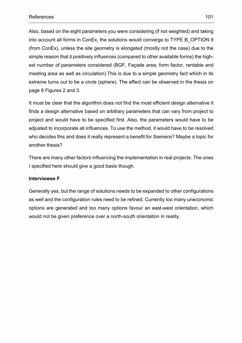
References 101
Also, based on the eight parameters you were considering (if not weighted) and taking
into account all forms in ConEx, the solutions would converge to TYPE B_OPTION 9
(from ConEx), unless the site geometry is elongated (mostly not the case) due to the
simple reason that it positively influences (compared to other available forms) the high-
est number of parameters considered (BGF, Façade area, form factor, rentable and
meeting area as well as circulation).This is due to a simple geometry fact which in its
extreme turns out to be a circle (sphere). The effect can be observed in the thesis on
page 8 Figures 2 and 3.
It must be clear that the algorithm does not find the most efficient design alternative it
finds a design alternative based on arbitrary parameters that can vary from project to
project and would have to be specified first. Also, the parameters would have to be
adjusted to incorporate all influences. To use the method, it would have to be resolved
who decides this and does it really represent a benefit for Siemens? Maybe a topic for
another thesis?
There are many other factors influencing the implementation in real projects. The ones
I specified here should give a good basis though.
Interviewee F
Generally yes, but the range of solutions needs to be expanded to other configurations
as well and the configuration rules need to be refined. Currently too many uneconomic
options are generated and too many options favour an east-west orientation, which
would not be given preference over a north-south orientation in reality.
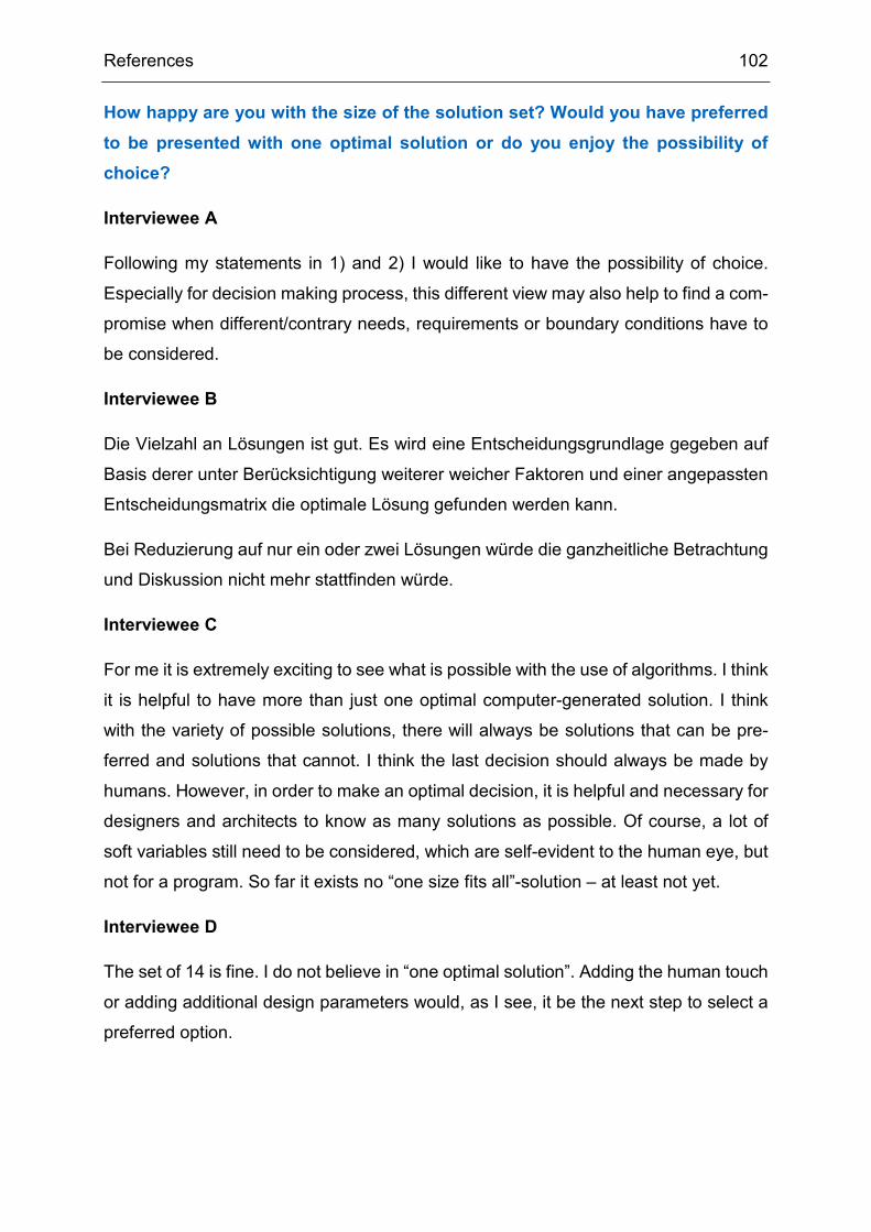
References 102
How happy are you with the size of the solution set? Would you have preferred to be presented with one optimal solution or do you enjoy the possibility of choice?
Interviewee A
Following my statements in 1) and 2) I would like to have the possibility of choice.
Especially for decision making process, this different view may also help to find a com-
promise when different/contrary needs, requirements or boundary conditions have to
be considered.
Interviewee B
Die Vielzahl an Lösungen ist gut. Es wird eine Entscheidungsgrundlage gegeben auf
Basis derer unter Berücksichtigung weiterer weicher Faktoren und einer angepassten
Entscheidungsmatrix die optimale Lösung gefunden werden kann.
Bei Reduzierung auf nur ein oder zwei Lösungen würde die ganzheitliche Betrachtung
und Diskussion nicht mehr stattfinden würde.
Interviewee C
For me it is extremely exciting to see what is possible with the use of algorithms. I think
it is helpful to have more than just one optimal computer-generated solution. I think
with the variety of possible solutions, there will always be solutions that can be pre-
ferred and solutions that cannot. I think the last decision should always be made by
humans. However, in order to make an optimal decision, it is helpful and necessary for
designers and architects to know as many solutions as possible. Of course, a lot of
soft variables still need to be considered, which are self-evident to the human eye, but
not for a program. So far it exists no “one size fits all”-solution – at least not yet.
Interviewee D
The set of 14 is fine. I do not believe in “one optimal solution”. Adding the human touch
or adding additional design parameters would, as I see, it be the next step to select a
preferred option.
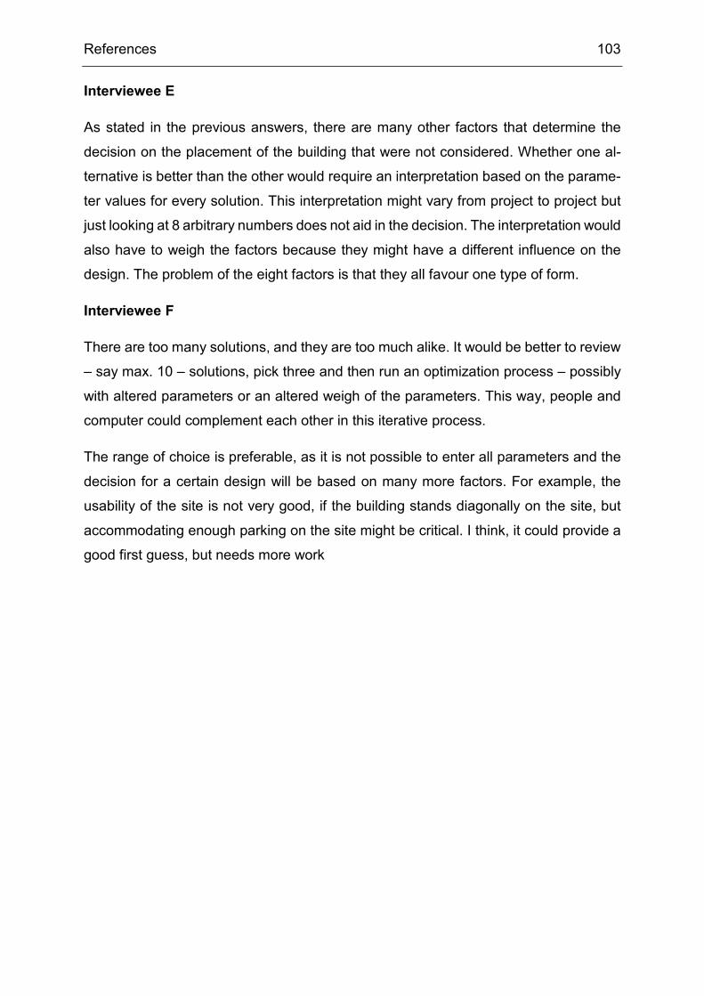
References 103
Interviewee E
As stated in the previous answers, there are many other factors that determine the
decision on the placement of the building that were not considered. Whether one al-
ternative is better than the other would require an interpretation based on the parame-
ter values for every solution. This interpretation might vary from project to project but
just looking at 8 arbitrary numbers does not aid in the decision. The interpretation would
also have to weigh the factors because they might have a different influence on the
design. The problem of the eight factors is that they all favour one type of form.
Interviewee F
There are too many solutions, and they are too much alike. It would be better to review
– say max. 10 – solutions, pick three and then run an optimization process – possibly
with altered parameters or an altered weigh of the parameters. This way, people and
computer could complement each other in this iterative process.
The range of choice is preferable, as it is not possible to enter all parameters and the
decision for a certain design will be based on many more factors. For example, the
usability of the site is not very good, if the building stands diagonally on the site, but
accommodating enough parking on the site might be critical. I think, it could provide a
good first guess, but needs more work
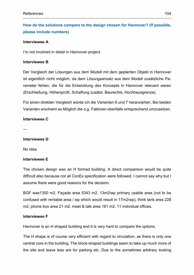
References 104
How do the solutions compare to the design chosen for Hannover? (If possible, please include numbers)
Interviewee A
I’m not involved in detail in Hannover project.
Interviewee B
Der Vergleich der Lösungen aus dem Modell mit dem geplanten Objekt in Hannover
ist eigentlich nicht möglich, da dem Lösungsansatz aus dem Modell zusätzliche Pa-
rameter fehlen, die für die Entwicklung des Konzepts in Hannover relevant waren
(Erschließung, Höhenprofil, Schaffung zusätzl. Baurechts, Hochhausgrenze).
Für einen direkten Vergleich würde ich die Varianten 6 und 7 heranziehen. Bei beiden
Varianten erscheint es Möglich die o.g. Faktoren ebenfalls entsprechend umzusetzen.
Interviewee C
---
Interviewee D
No idea.
Interviewee E
The chosen design was an H formed building. A direct comparison would be quite
difficult also because not all ConEx specification were followed. I cannot say why but I
assume there were good reasons for the decision.
BGF was1350 m2, Façade area 5343 m2, 13m2/wp primary usable area (not to be
confused with rentable area / wp which would result in 17m2/wp), think tank area 228
m2, phone box area 21 m2, meet & talk area 181 m2, 11 individual offices.
Interviewee F
Hannover is an H shaped building and it is very hard to compare the options.
The H shape is of course very efficient with regard to circulation, as there is only one
central core in the building. The block-shaped buildings seem to take up much more of
the site and leave less are for parking etc. Due to the sometimes arbitrary looking

References 105
placement, the site gets cut into some inefficient shapes, where is would be hard to
accommodate parking etc.
I think, several options should not have “survived”: option 1, 3, 4, 8, 10 and 13 have
either two or even three cores which are placed at the end of the building with another
staircase next to them. This does not make sense. But I guess, it shows the limitations,
if you don’t tell the machine that this is not an option, it may think, it is a good one!
I would have liked to see more options which are placed parallel to the main street like
the actual design.

References 106
If you had to pick one or two of the solutions, which ones would be your favorite? Why?
Interviewee A
I’m not involved in detail in Hannover project.
Interviewee B
Mein Favoriten sind 5 und 6. Beide erscheinen sehr kompakt und wirtschaftlich.
Interviewee C
---
Interviewee D
Looking only at the existing parameters I would tend to focus less on build space and
façade area and lean more towards functional parameters such as circulation and
meeting area/WP as I believe these parameters leads to a “better building”. I believe it
would depend on the parameters not included in the parametric set of goals.
Interviewee E
If I had to pick, I would probably go for #12 or #9. The elongated alternatives block a
lot of the panoramic view of the site and I prefer symmetry in regard to neighbouring
sites in this scenario since I do not have information on neighbouring buildings and the
landscape developments around the building. It seems safer to have a more centrally
positioned building.
Interviewee F
Probably one of the solutions which has a single core.