Embed Size (px)
Citation preview

HAL Id: hal-01579519https://hal.archives-ouvertes.fr/hal-01579519
Submitted on 31 Aug 2017
HAL is a multi-disciplinary open accessarchive for the deposit and dissemination of sci-entific research documents, whether they are pub-lished or not. The documents may come fromteaching and research institutions in France orabroad, or from public or private research centers.
L’archive ouverte pluridisciplinaire HAL, estdestinée au dépôt et à la diffusion de documentsscientifiques de niveau recherche, publiés ou non,émanant des établissements d’enseignement et derecherche français ou étrangers, des laboratoirespublics ou privés.
Design study of the coupling of an air gap membranedistillation unit to an air conditioner
Ahmadou Tidiane Diaby, Paul Byrne, Patrick Loulergue, Béatrice Balannec,Anthony Szymczyk, Thierry Maré, Ousmane Sow
To cite this version:Ahmadou Tidiane Diaby, Paul Byrne, Patrick Loulergue, Béatrice Balannec, Anthony Szymczyk, etal.. Design study of the coupling of an air gap membrane distillation unit to an air conditioner.Desalination, Elsevier, 2017, 420, pp.308 - 317. �10.1016/j.desal.2017.08.001�. �hal-01579519�
Manuscript Details
Manuscript number DES_2017_1223
Title Design study of the coupling of an air gap membrane distillation unit to an airconditioner
Article type Full Length Article
Abstract
This work presents the design of a membrane distillation (MD) unit coupled to a refrigeration device. The operation ofan MD pilot plant is first tested then modelled using EES software. The range of hot water feed temperature providedby the condenser of the refrigeration device may vary from 25 to 65 °C as needed by the MD unit. The results of theexperimental study enable to validate a 1D theoretical model with a maximum deviation of ± 6%. This model is coupledto a heat pump model to simulate the operation of a coupled machine. The system performance is studied followingtwo scenarios. In Scenario 1 (continuous mode), the system is connected to a seawater network. In Scenario 2 (batchmode), the seawater reservoir is filled up manually every day. The simulation study shows that the increase of the feedwater temperature enhances significantly the produced permeate flux but decreases the performance of the heatpump. This system exhibits high exergy efficiency and GOR for a high feed water temperature. Exergy efficiency andgained output ratio (GOR) decrease as the water flow increases and the hot water temperature decreases.Conversely, the coefficient of performance (COP) of the refrigerator increases.
Keywords air conditioner; coupling; air gap membrane distillation
Corresponding Author Paul Byrne
Order of Authors Ahmadou Diaby, Paul Byrne, Patrick LOULERGUE, Beatrice Balannec, AnthonySZYMCZYK, Thierry Maré, Ousmane Sow
Suggested reviewers A.G Fane, Wojciech Kujawski, NALAN KABAY
Submission Files Included in this PDF
File Name [File Type]
Cover Letter.doc [Cover Letter]
Diaby Desalination.docx [Manuscript File]
To view all the submission files, including those not included in the PDF, click on the manuscript title on your EVISEHomepage, then click 'Download zip file'.
Paul Byrne Rennes, 09/06/17IUT Génie CivilCivil & Mechanical Engineering Laboratory3 Rue du Clos CourtelBP 9042235704 Rennes Cedex [email protected] : +33 2 23 23 42 97Fax : +33 2 23 23 40 51
To editor and reviewers of Desalination
Subject: Cover letter
Dear Editor, dear reviewers,
Please find in this submission a full-length article on the design study of the coupling of a cooling device with an air gap membrane distillation unit. This work was presented at the MEMDES 2017 conference in Las Palmas de Gran Canaria. The first author is Ahmadou Diaby, a PhD student under the co-supervision of researchers from LGCGM and ISCR laboratories from Rennes France and the LEA of Dakar Senegal.
Best regards,
Paul Byrne

1
Design study of the coupling of an air gap membrane distillation unit to an air conditioner
Ahmadou Tidiane Diaby1,2, Paul Byrne1*, Patrick Loulergue3, Béatrice Balannec3, Anthony Szymczyk3, Thierry Maré1, Ousmane Sow2
1 Laboratoire Génie Civil Génie Mécanique, INSA de Rennes et Université de Rennes 1, France2 Laboratoire d’Energétique Appliquée, Ecole Supérieure Polytechnique, Université Cheikh Anta Diop de
Dakar, Sénégal3 Institut des Sciences Chimiques de Rennes (UMR CNRS 6226), Université de Rennes 1, ENSCR, France
Abstract
This work presents the design of a membrane distillation (MD) unit coupled to a refrigeration device. The operation of an MD pilot plant is first tested then modelled using EES software. The range of hot water feed temperature provided by the condenser of the refrigeration device may vary from 25 to 65 °C as needed by the MD unit. The results of the experimental study enable to validate a 1D theoretical model with a maximum deviation of ± 6%. This model is coupled to a heat pump model to simulate the operation of a coupled machine.
The system performance is studied following two scenarios. In Scenario 1 (continuous mode), the system is connected to a seawater network. In Scenario 2 (batch mode), the seawater reservoir is filled up manually every day. The simulation study shows that the increase of the feed water temperature enhances significantly the produced permeate flux but decreases the performance of the heat pump. This system exhibits high exergy efficiency and GOR for a high feed water temperature. Exergy efficiency and gained output ratio (GOR) decrease as the water flow increases and the hot water temperature decreases. Conversely, the coefficient of performance (COP) of the refrigerator increases.
Keywords: air conditioner, coupling, air gap membrane distillation
1. Introduction
The building sector accounts for 40% of the world’s energy consumption. The number of air conditioning and refrigeration devices is estimated at 4 billion units consuming 17 % of global electric energy [1]. When installed in high buildings, air conditioners heat air flowing through the outdoor condensers. The air density increases and the air tends to flow up near another condenser to be heated again. This phenomenon is partly responsible for the urban heat island effect. The proximity of buildings and their cooling equipment creates hot outdoor environment provoking higher cooling demands and lower performance of air conditioners. In addition, the world population is growing, which leads to an increase of the needs of commercial and domestic refrigeration and air conditioning as well as in drinking water. Human activities lead to the decrease of available water resources because of pollutions or their use for farming and industrial activities. Over 40% of the world’s population living in watersheds by serious water shortages, the demand in terms of water resource levy should increase by around 55% by 2050 [2]. The desalination of seawater or brackish water is often a solution to the lack of fresh water.
Numerous studies deal with cold production for air conditioning or refrigeration firstly and secondly the desalination of seawater. However, there are very few papers in the literature studying the coupling of cooling systems and desalination in order to produce simultaneously a cooling capacity and fresh water (see [3] for a recent review). In addition, the simulation study of a membrane distillation system for seawater desalination coupled to a heat pump was already conducted but needs to be improved in terms of system sizing and operating conditions [4]. An optimization study for the design of thermal distillation systems thermally coupled to treatment facilities was carried out by Gonzalez-Bravo et al. [5] to obtain simultaneously the optimization on a minimum cost criterion of the thermal distillation unit and the heat exchange network that integrates heating and cooling in the process facility.
Figure 1 classifies the main desalination techniques are into two categories: membrane processes and thermal processes. Figure 1 also recalls the percentage of total volume of desalinated water production for the three main systems, which are reverse osmosis (RO), multi-stage flash distillation (MSF) and multiple-effect distillation (MED). The other systems account for the remaining 6 %. The degree of compatibility of desalination techniques with heat pumps is evaluated in Table 1. It appears clearly that the operation of electrodialysis (ED) is not related to heat. The temperature has very low influence on the operation of RO. These two methods of membrane desalination technology are not suited to the coupling with heat pumps. MED and MD appear to be systems

2
compatible with classic heat pumps. The operating temperature range of MSF is high in comparison to that produced by the heat pump that can range from 25 °C to 65 °C. For thermal vapour compression (TVC), the temperature range corresponds to that of a heat pump, but this process does not have a refrigerating effect.
Figure 1: Classification of commonly used desalination technologies
Table 1: Compatibility assessment of desalination systems with refrigerating devicesSystems Process Operating
temperatureCompatibility
with a refrigerating deviceED Mechanical / Membrane Not appropriate NoRO Mechanical / Membrane Low influence No
MED Thermal 70 °C – 80 °C Yes, with a high temperature HP
MSF Thermal 80 °C – 120 °C NoMD Thermal / Membrane 40 °C – 80 °C Yes, with a classic HPTVC Mechanical / Thermal 60 °C – 70 °C No refrigerating effect
Membrane distillation is both a thermal and a membrane process. MD can produce high-quality pure water by utilizing a porous hydrophobic membrane to separate a feed compartment and a permeate compartment. The MD process is most suitable due to the low operating temperatures, compatible with conventional air conditioning units. Low-grade waste heat or renewable energy might be favourably used for seawater desalination using membrane distillation [6]. MD is a thermal membrane process using the vapour pressure gradient created between a hot stream and a cold stream as the driving force. Four classic configurations of MD are usually encountered in the literature, which differ by the nature of the permeate management [7-8]: direct contact membrane distillation (DCMD), air gap membrane distillation (AGMD), vacuum membrane distillation (VMD) and sweeping-gas membrane distillation (SGMD). In all MD configurations, one side of the hydrophobic membrane is in contact with the hot feed solution. The other side is in contact with cold permeate for DCMD, air gap for AGMD, vacuum for VMD and gas for SGMD. DCMD is the easiest and simplest configuration [7]. In this process, the heat loss by conduction is high and it presents a high risk of wetting of the membrane. AGMD is the most versatile of all configurations because of its air gap [9]. It is characterized by the lowest thermal losses and by a lower risk of wetting and fouling of the membrane. The recovery of the heat to preheat the feed solution is easy with DCMD and AGMD. SGMD is known for its low temperature polarization and relatively low permeate flux [7]. VMD has a low loss of thermal conductivity and resistance to mass transfer in the boundary layer with a high permeate flux [10], it has a very high risk of wetting the membrane [11]. Additional energy is consumed for the vacuum pump in VMD and for ventilation in SGMD. The heat recovery is very difficult with these two configurations and the set-up is more complex due to the need of an external condenser. Following this screening of desalination systems, AGMD was chosen for the coupled system due to its simplicity.
Therefore, the objective of this study is to couple a cooling device with an AGMD unit for the simultaneous production of cold air and fresh water by desalination. The thermodynamic cycle of the cooling device and the

3
AGMD unit were modelled using EES software [12]. Each component of the refrigeration circuit (compressor, condenser, expansion valve and evaporator) is modelled. Based on the experimental results obtained with an AGMD pilot plant (different machine from the coupled system), the model is first validated. It is subsequently used to predict the performance, in terms of permeate flux, energy and exergy efficiency, of the coupled system that produces cooling energy and distilled water.
2. Description of the coupled system
The idea is to recover the heat lost towards the environment by a refrigeration equipment or an air conditioning equipment to produce fresh water (Figure 2). The coupled system is sized using a small air conditioner with a cooling capacity of 2.5 kW. The evaporator supplies cooling energy. This heat exchanger is here a roll-bond in which the refrigerant gradually changes from the liquid state to the gaseous state by absorbing heat from the medium to be cooled (heat source). The compressor is a mechanical device that sucks the gaseous refrigerant coming from the evaporator at low temperature and pressure, compresses it to a higher level of temperature and pressure and then delivers it to the condenser. The condenser is a heat exchanger that supplies the latent heat contained in the refrigerant in the gaseous state issuing from the compressor by liquefying it. The expansion valve reduces the temperature and the pressure of the refrigerant coming from the condenser before it is injected into the evaporator.
A plate heat exchanger (HX) is positioned between the air conditioner and the unit MD to recover the quantity of heat contained in the brine by preheating the feed solution and slow the progression of the feed temperature in the tank. A pump drives successively the feed solution in the cold channel of the MD unit, in the condenser of the air conditioning to heat the feed solution, then in the hot channel of the MD unit where the flux is divided between the permeate flux and the brine flux, which is slightly more concentrated in salt. The brine flows finally back to the feed tank. Pre-treatment and post-treatment are not dealt with in this study. The system is operated with mixed solutions of pure water and salts.
Figure 2: Scheme of the air conditioner coupled to the AGMD unit with heat exchanger (Scenario 2)
Two following scenarios are studied with this coupled system.- In Scenario 1, the system is connected to a network of seawater instead of the water tank of Figure 2.
The brine is directly discharged into the sea (open loop continuous operation). The recovery heat exchanger is used to preheat the feed seawater with the heat left in the brine. This scenario can be applied to hotels or office buildings installed close to the sea using refrigeration or air conditioning. The inlet temperature of the cold channel (Tc,in) is considered constant for a given test.

4
- Scenario 2 corresponds to the configuration shown in Figure 2 (batch mode). It is a system with a closed loop function that can be used in rural areas. The tank is assumed to be filled up regularly with a new amount of sea water or brackish water. An initial tank volume of 100 L was assumed acceptable regarding a daily filling up. A dynamic model is useful for evaluating the performance of the system because the salt concentration, the temperature and the mass of the reservoir evolve over time. A coefficient equal to 0.2 kW.K-1 is applied to take into account the heat loss of the tank volume towards the environment because it continuously recovers the hotter brine.
3. Numerical modelling
3.1. Air conditioner model
The results of experimental tests on an air-to-water heat pump working with propane (R290) were used to validate the numerical models of the components [13]. The compressor power and the coefficient of performance (COP) are predicted within 5% of error. The coupled system is sized with a small air conditioner with nominal heating and cooling capacities of 2.5 kW and 2 kW respectively for Tcd = 40 °C and Tev = 0 °C. The expansion valve is simply modelled by the conservation of the enthalpy through the expansion process. The models of compressor and heat exchangers are presented hereafter.
3.1.1. Compressor model
The compressor model is built using data tables provided by the manufacturer reporting the COP, the cooling capacity and the electric power consumption as a function of evaporating and condensing pressures. Equation 1 determines the refrigerant flow rate from the fluid density, volumetric efficiency and swept volume. Equation 2 is used to calculate the electrical power absorbed by the ideal mechanical power according to isentropic compression and the isentropic efficiency of the compressor.
(1)𝑊𝑖𝑠 = 𝜌 ∙ 𝜂𝑣𝑜𝑙 ∙ 𝑉𝑠𝑤𝑒𝑝𝑡 ∙ ∆ℎ𝑐𝑜𝑚𝑝
(2)𝑊𝑐𝑜𝑚𝑝 =𝑊𝑖𝑠
𝜂𝑖𝑠
The volumetric and isentropic efficiency are given by equations 3 and 4 as a function of the compression ratio (ratio of high pressure over low pressure), evaporation and condensation temperatures and the polytropic coefficient .
(3)𝜂𝑖𝑠 =‒ 0,001𝜎3 + 0,026𝜎2 ‒ 0,25𝜎 ‒ 0,014𝑇𝑒𝑣 + 0,0108𝑇𝑐𝑑 + 0,7512
(4)𝜂𝑣𝑜𝑙 =‒ 0,1290𝜎𝛾 + 0,1257𝜎 + 0,9010
3.1.2. Heat exchangers model
The heat exchanger models use the logarithmic average of the temperature difference method (DTLM). The heat exchanged can be calculated using equations 5 to 7. In the case of the external air evaporator, a correction factor F is taken into account due to cross-flow fluids. The resolution of the system of equations 5 to 7 makes it possible to calculate the refrigerant operating pressures as well as the outlet temperatures. The global heat exchange coefficients (U values for the evaporator and the condenser) were calculated using correlations on the convective heat exchange of the fluids as a function of their temperatures [14-15].
(5)𝑄 = 𝑈 ∙ 𝑆 ∙ 𝐷𝑇𝐿𝑀
(6)𝑄 = 𝑚𝑠𝑜 ∙ 𝐶𝑝𝑠𝑜
∙ ∆𝑇𝑠𝑜
(7)𝑄 = 𝑚𝑟 ∙ ∆ℎ𝑟
5
3.2. AGMD unit
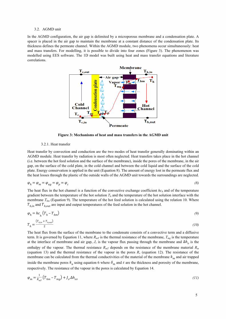
In the AGMD configuration, the air gap is delimited by a microporous membrane and a condensation plate. A spacer is placed in the air gap to maintain the membrane at a constant distance of the condensation plate. Its thickness defines the permeate channel. Within the AGMD module, two phenomena occur simultaneously: heat and mass transfers. For modelling, it is possible to divide into four zones (Figure 3). The phenomenon was modelled using EES software. The 1D model was built using heat and mass transfer equations and literature correlations.
Figure 3: Mechanisms of heat and mass transfers in the AGMD unit
3.2.1. Heat transfer
Heat transfer by convection and conduction are the two modes of heat transfer generally dominating within an AGMD module. Heat transfer by radiation is most often neglected. Heat transfers takes place in the hot channel (i.e. between the hot feed solution and the surface of the membrane), inside the pores of the membrane, in the air gap, on the surface of the cold plate, in the cold channel and between the cold liquid and the surface of the cold plate. Energy conservation is applied in the unit (Equation 8). The amount of energy lost in the permeate flux and the heat losses through the plastic of the outside walls of the AGMD unit towards the surroundings are neglected.
(8)𝜑ℎ = 𝜑𝑚 = 𝜑𝑎𝑔 = 𝜑𝑝 = 𝜑𝑐
The heat flux in the hot channel is a function of the convective exchange coefficient hch and of the temperature gradient between the temperature of the hot solution Th and the temperature of the hot solution interface with the membrane Thm (Equation 9). The temperature of the hot feed solution is calculated using the relation 10. Where
and are input and output temperatures of the feed solution in the hot channel.𝑇ℎ,𝑖𝑛 𝑇ℎ,𝑜𝑢𝑡
(9)𝜑ℎ = ℎ𝑐ℎ (𝑇ℎ ‒ 𝑇ℎ𝑚)
(10)𝑇ℎ =(𝑇ℎ,𝑖𝑛 + 𝑇ℎ,𝑜𝑢𝑡)
2
The heat flux from the surface of the membrane to the condensate consists of a convective term and a diffusive term. It is governed by Equation 11, where RmT is the thermal resistance of the membrane, Tmg is the temperature at the interface of membrane and air gap, Jv is the vapour flux passing through the membrane and is the ∆ℎ𝑣enthalpy of the vapour. The thermal resistance RmT depends on the resistance of the membrane material Rm (equation 13) and the thermal resistance of the vapour in the pores Rv (equation 12). The resistance of the membrane can be calculated from the thermal conductivities of the material of the membrane and air trapped 𝑘𝑚inside the membrane pores using equation 6 where and are the thickness and porosity of the membrane, 𝑘𝑎 𝛿𝑚 𝜀respectively. The resistance of the vapour in the pores is calculated by Equation 14.
(11)𝜑𝑚 =1
𝑅𝑚𝑇 (𝑇ℎ𝑚 ‒ 𝑇𝑚𝑔) + 𝐽𝑣.∆ℎ𝑒𝑣

6
(12)𝑅𝑚𝑇 =𝑅𝑚 𝑅𝑣
𝑅𝑚 + 𝑅𝑣
(13)𝑅𝑚 =𝛿𝑚
𝜀 . 𝑘𝑎 + (1 ‒ 𝜀) . 𝑘𝑚
(14)𝑅𝑣 =1
𝐽𝑣 . 𝐶𝑝𝑣
The heat flux through the air gap is assumed solely convective and carried by the water vapour and is calculated using equation 15 where and are the thermal resistance of the air gap and temperature of permeate, 𝑅𝑎𝑔 𝑇𝑝respectively. The thermal resistance of the air gap can be calculated through equation 16. , and are the 𝛿𝑎𝑔 𝛿𝑝 𝛿𝑠air gap, permeate and spacer thicknesses, respectively. is the conductivity of the spacer, is the void volume 𝑘𝑠 𝑉𝑣𝑠of the spacer and is the total volume of the spacer. The permeate thickness is determined by equation 17, where 𝑉𝑠
, and are liquid water and vapour densities and vapour viscosity, respectively, and is the acceleration 𝜌𝑤 𝜌𝑣 𝜇𝑣 𝑔of gravity.
(15)𝜑𝑎𝑔 =1
𝑅𝑎𝑔 (𝑇𝑚𝑔 ‒ 𝑇𝑝)
(16)1
𝑅𝑎𝑔=
1𝑅𝑣
+(𝛿𝑎𝑔 ‒ 𝛿𝑝)
𝑘𝑎+
𝛿𝑠
(1 ‒ 𝑉𝑣𝑠/𝑉𝑠) 𝑘𝑠
(17)𝛿𝑝 = [3 𝜇𝑣∫𝑥0𝐽𝑣(𝑥)𝑑𝑥
𝑔𝜌𝑤(𝜌𝑤 ‒ 𝜌𝑣) ]1/3
The heat flux from the interface of the condensation surface to the interface between the cooling solution and the metal plate can be translated by equation 18 where and are the thermal conductivity of the plate, the plate 𝑘𝑝 𝛿𝑝thickness and is the temperature at the interface of the cold solution and the plate.𝑇𝑝𝑐
(18)𝜑𝑝 =𝑘𝑝
𝛿𝑝 (𝑇𝑝𝑐 ‒ 𝑇𝑝) + 𝐽𝑣.∆ℎ𝑐𝑑
The heat flux in the boundary layer of the cold channel can be expressed by equation 19, where and are the ℎ𝑐 𝑇𝑐heat transfer coefficient and the temperature of the cold solution in the cold channel. The mean temperature of the cold solution is calculated using equation 20.
(19)𝜑𝑐 = ℎ𝑐𝑐 (𝑇𝑝 ‒ 𝑇𝑐)
(20)𝑇𝑐 =(𝑇𝑐, 𝑖𝑛 + 𝑇𝑐, 𝑜𝑢𝑡)
2
The convective heat transfer coefficients and can be calculated by equation 21 where is the hydraulic ℎ𝑐ℎ ℎ𝑐𝑐 𝑑ℎdiameter, is the thermal conductivity and is the Nusselt number and can be determined by the correlations 𝑘 𝑁𝑢of Table 2 depending on the Reynolds number.
(21)ℎ𝑐 =𝑁𝑢 𝑘
𝑑ℎ
Table 2: Convective heat transfer coefficients used in the MD unitAuthor Correlation Validity domain
Pangarkar [16] 𝑁𝑢 = 0.023 𝑅𝑒0,8 𝑃𝑟1/3( 𝜇𝜇𝑤
)0.14
2500 < 𝑅𝑒 < 1.25 105
Aryapratama [17] 𝑁𝑢 = 3.36 +0.036 𝑅𝑒 𝑃𝑟(𝑑ℎ/𝐿)
1 + 0.0011 (𝑅𝑒 𝑃𝑟/𝐿)0.8 𝑅𝑒 > 2100
Khayet [18] 𝑁𝑢 = 0.116(𝑅𝑒1/3 ‒ 125) 𝑃𝑟1/3[1 + (𝑑ℎ/𝐿)2/3] Transitional regime
Phattaranawik [19] 𝑁𝑢 = 0.664 𝑅𝑒0.5 𝑃𝑟0.33(𝑑ℎ/𝐿)0.5
Essalhi [20] 𝑁𝑢 = 1.86(𝑅𝑒Pr 𝑑ℎ/𝐿)1/3 Laminar flow regime

7
3.2.2. Mass transfer
Mass transfer through the membrane depends on the vapour pressure difference between the two sides of the membrane. The relationship between the mass transfer, the vapour pressure difference and the effect of salt concentration in the solution is given by equation 22, where and are the vapour pressures at the surface of 𝑃ℎ𝑚 𝑃𝑝the membrane in the boundary layer of the hot channel and in the air gap near the surface of the cold plate, respectively. is the activity coefficient and is the water fraction of the solution. Pressures and can be α 𝛽 𝑃ℎ𝑚 𝑃𝑝evaluated using the Antoine equation (equation 23). The activity coefficient of an aqueous solution can be 𝛼calculated by equation 24. The permeability of the membrane or the mass transfer coefficient of equation 22 𝐵𝑤
is given in equation 25. , , and are the molecular weight of water, the gas constant, the absolute 𝑀𝑤 𝑅 ∗ 𝑇𝑚 𝑃temperature of the membrane and the total pressure inside the pores, respectively. is the thermal diffusivity 𝐷𝑣𝑎of water vapour in the air gap and is the tortuosity of the membrane and can be calculated by equation 26. The 𝜏product can finally be calculated by equation 27. 𝑃𝐷𝑣𝑎
(22)𝐽𝑤 = 𝐵𝑤(𝛼 𝛽 𝑃ℎ𝑚 ‒ 𝑃𝑝)
(23)𝑃 = 𝑒𝑥𝑝(23,1964 ‒3816,44
𝑇 ‒ 46.13)(24)𝛼 = 1 ‒ 0.5 𝑋𝑁𝑎𝐶𝑙 ‒ 10 𝑋 2
𝑁𝑎𝐶𝑙
(25)𝐵𝑤 =𝜀 𝑀𝑤𝑃 𝐷𝑣𝑎
𝑅 ∗ 𝑇𝑚(𝛿𝑚𝜏 + 𝛿𝑎𝑔)|𝑃𝑎|𝑙𝑛,𝑎
(26)𝜏 =2 ‒ 𝜀
𝜀
(27)𝑃𝐷𝑣𝑎 = 1,895 × 10 ‒ 5𝑇𝑚2.027
The mass balance of the AGMD module is given by equation 28, where , and are the mass m𝑠𝑤,𝑖𝑛 m𝑠𝑤,𝑜𝑢𝑡 m𝑝flow rate, feed solution inlet, feed solution out and permeate, respectively.
(28)𝑚𝑠𝑤,𝑖𝑛 = 𝑚𝑠𝑤,𝑜𝑢𝑡 + 𝑚𝑝
3.2.3. Dynamic behaviour
In Scenario 2 (see section 2), the mechanisms of heat and mass transfers strongly depend on the initial mass and the initial temperature of the water tank. The evolution of these quantities is a function of time for the system studied. The mass of the tank is calculated as following:
(29)𝑚𝑡𝑎𝑛𝑘 = 𝑚𝑖, 𝑡𝑎𝑛𝑘 ‒ ∫𝑡0𝑚𝑝𝑑𝑡
The heat transfer in the balance tank containing the feed is estimated by equation 30. The UAtank value is the product of a heat exchange coefficient and a surface area evaluating the heat losses of the tank.
(30)𝐶𝑝𝑡𝑎𝑛𝑘∆𝑇𝑑𝑚𝑡𝑎𝑛𝑘
𝑑𝑡 =‒ 𝑚𝑓,𝑖𝑛𝐶𝑝𝑓,𝑖𝑛𝑇𝑓,𝑖𝑛 + 𝑚𝑓,𝑜𝑢𝑡𝐶𝑝𝑓,𝑜𝑢𝑡𝑇𝑓,𝑜𝑢𝑡 ‒ 𝑈𝐴𝑡𝑎𝑛𝑘 (𝑇𝑡𝑎𝑛𝑘 ‒ 𝑇𝑎𝑚𝑏)
The evolution of the tank temperature can be calculated by equation 31. Ti,tank corresponds to the initial temperature of the feed solution in the tank.
(31)𝑇𝑡𝑎𝑛𝑘 = 𝑇𝑖, 𝑡𝑎𝑛𝑘 + ∫𝑡0
∆𝑇𝛿𝑡 𝑑𝑡
The water salinity in the tank also varies with time. During the operation, distilled water is produced. This amount of water does not reintegrate the water tank while the amount of salts stays constant because on the contrary, the brine flows back to the tank. Equation 32 calculates the evolution of the salinity with time.
(32)𝑆 =𝑚𝑠𝑤
𝑚𝑡𝑎𝑛𝑘

8
3.3. System performance assessment
3.3.1. Cooling device
In these studies, the compressor consumption and the coefficient of performance (COP) are evaluated. We define the COP as the ratio of the cooling capacity to the electric power absorbed by the compressor (equation 33).
(33)𝐶𝑂𝑃 =𝛷𝑒𝑣
𝑊𝑒𝑙𝑒𝑐
3.3.2. Desalination unit
For desalination units, the performance is evaluated by the amount of energy consumed with respect to the amount of freshwater produced. The GOR (Gained Output Ratio) corresponds to the ratio of the amount of energy necessary to vaporize the permeate flux divided by the heat consumption GOR is used to measure the energy consumption of the process and it can be described by [21] (equation 34).
(34)𝐺𝑂𝑅 =𝑚𝑝 ∆ℎ𝑣
𝑚𝑠𝑤,𝑖𝑛𝐶𝑝𝑆𝑤,𝑖𝑛(𝑇ℎ,𝑖𝑛 ‒ 𝑇ℎ,𝑜𝑢𝑡)
3.3.3. Exergy analysis
An exergy analysis is performed to convert the energy amounts from different forms (thermal, electric, chemical) and to calculate an exergy efficiency [22]. The exergy rate available in a water flux comprises thermal and chemical (ech) terms and is evaluated by equation 35. This equation can be used to determine the exergy rate of the brine sw,out. The exergy rate of a thermal flux th, such as the cooling energy, is calculated using equation Ex Ex36. The reference state is defined by mean ambient conditions (T0 = 20 °C and P0 = 1 bar). The exergy efficiency of the system is given by equations 37 and 38. The economical exergy efficiency takes into account the useful production and the charged inputs to the system. The process exergy efficiency regards all inputs and outputs with the idea that every stream has a potential value.
(35)𝐸𝑥𝑤 = 𝑚[(ℎ ‒ ℎ0) ‒ 𝑇0(𝑠 ‒ 𝑠0) + 𝑒𝑐ℎ](36)𝐸𝑥𝑡ℎ = 𝛷𝑒𝑣|1 ‒
𝑇0
𝑇 |(37)𝜂𝑒𝑥,𝑒𝑐𝑜 =
𝐸𝑥𝑡ℎ + 𝐸𝑥𝑤,𝑜𝑢𝑡
𝐸𝑥𝑒𝑙𝑒𝑐 + 𝐸𝑥𝑝𝑢𝑚𝑝
(38)𝜂𝑒𝑥,𝑝𝑟𝑜 =𝐸𝑥𝑡ℎ + 𝐸𝑥𝑤,𝑜𝑢𝑡 + 𝐸𝑥𝑠𝑤,𝑜𝑢𝑡
𝐸𝑥𝑒𝑙𝑒𝑐 + 𝐸𝑥𝑝𝑢𝑚𝑝 + 𝐸𝑥𝑠𝑤,𝑖𝑛
4. Results and discussion
4.1. Experimental results
The experimental tests were carried out on an AGMD pilot plant (Xzero AB, Sweeden) (Figure 4). The pilot plant is equipped with a 25-litre feed tank and a PTFE membrane (Gore, USA) with the same characteristics as reported in Table 3 and with a surface area of 0.195 m². Several parameters were studied, such as hot feed temperature, feed and coolant flow rates and air gap thickness with a model solution at 35 g/l NaCl. The feed temperature varies from 25 to 65 °C. The range of feed flow rate and coolant flow rate is from 2 to 5 l/min. The air gap thickness is 1.04 mm. The mean temperature of the cold fluid is the one of the chilled water network of the building, at 16 °C for all tests. The permeate is sampled every 20 minutes and then weighed with a precision scales. The permeate conductivity is measured with a conductivity meter in order to calculate the salt rejection using equation 39.κp
(39)𝑠𝑎𝑙𝑡 𝑟𝑒𝑗𝑒𝑐𝑡𝑖𝑜𝑛 =𝜅𝑠𝑤,𝑖𝑛 ‒ 𝜅𝑝
𝜅𝑠𝑤,𝑖𝑛

9
Table 3: Membrane characteristics (according to supplier)Property Value
Thickness (mm) 0.28 Pore size (µm) 0.2 Porosity (%) 80 Tortuosity (-) 1.5
Figure 4: Scheme of the AGMD pilot plant
4.1.1. Long term performance
A test of a total operating time of about 30 hours was performed during four consecutive days with real seawater sampled in St Malo, France. For this long-term test, the same quantity of seawater as the produced permeate mass is added to the initial seawater in the tank every 20 minutes. This method concentrates the hot feed solution. Figure 5 shows the evolution of the electrical conductivity in the reservoir containing the feed solution.
0 300 600 900 1200 1500 180050
60
70
80
90
100
Operating time (min)
Feed
cond
uctiv
ity(m
S/cm
)
Figure 5: Evolution of the conductivity of the feed solution in the tank
10
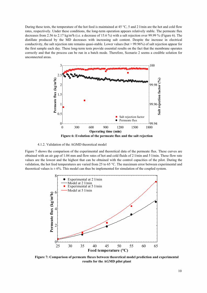
During these tests, the temperature of the hot feed is maintained at 45 °C, 5 and 2 l/min are the hot and cold flow rates, respectively. Under these conditions, the long-term operation appears relatively stable. The permeate flux decreases from 2.56 to 2.17 kg/m²h (i.e. a decrease of 15.6 %) with a salt rejection over 99.99 % (Figure 6). The distillate produced by the MD decreases with increasing salt content. Despite the increase in electrical conductivity, the salt rejection rate remains quasi-stable. Lower values (but > 99.96%) of salt rejection appear for the first sample each day. These long-term tests provide essential results on the fact that the membrane operates correctly and that the process can be run in a batch mode. Therefore, Scenario 2 seems a credible solution for unconnected areas.
0 300 600 900 1200 1500 1800
0
0.5
1
1.5
2
2.5
3
99.94
99.96
99.98
100
Operating time (min)
Perm
eate
flux
(kg/
m²h
)
Permeate flux
Salt
reje
ctio
nfa
ctor
(%)
Salt rejection factor
Figure 6: Evolution of the permeate flux and the salt rejection
4.1.2. Validation of the AGMD theoretical model
Figure 7 shows the comparison of the experimental and theoretical data of the permeate flux. These curves are obtained with an air gap of 1.04 mm and flow rates of hot and cold fluids of 2 l/min and 5 l/min. These flow rate values are the lowest and the highest that can be obtained with the control capacities of the pilot. During the validation, the hot feed temperatures are varied from 25 to 65 °C. The maximum error between experimental and theoretical values is ± 6%. This model can thus be implemented for simulation of the coupled system.
25 30 35 40 45 50 55 60 650
2
4
6
8
Feed temperature (°C)
Perm
eate
flux
(kg/
m²h
)
Experimental at 2 l/minModel at 2 l/minExperimental at 5 l/minModel at 5 l/min
Figure 7: Comparison of permeate fluxes between theoretical model prediction and experimental results for the AGMD pilot plant

11
4.2. Simulation results with the coupled system
The results of the coupled system are calculated with a membrane area of 1 m². The properties of the membrane remain the same as in Table 3.
4.2.1. Effect of the heat source temperature at the evaporator of the cooling device
The effect of the heat source temperature of the cooling device is evaluated using Scenario 1. The heat source varies from -10 °C to 25 °C, with an air gap thickness of 1.04 mm an flow rate of 2 l/min and different initial tank feed temperatures. Figure 8 shows the permeate flux as a function of the temperature of the heat source and the initial feed temperature of the tank. The permeate flux is very sensitive to the variation of the heat source temperature. It is observed that the permeate flux increases as the heat source temperature increases. If the ambient air temperature increases, the refrigerant evaporates at a higher temperature, this will allow the compressor to draw in the refrigerant without consuming a too high amount of electrical energy. When the temperature of the heat source decreases, the COP, the cooling and heating capacities decrease because the compressor consumes more of its energy to build up pressure than to send refrigerant flow rate. The MD unit receives colder seawater in the hot channel and the temperature and vapour gradient is lower. Therefore, the permeate flux decreases with the lower cooling capacity when considering the same refrigerating machine. This result shows that air conditioning is more suitable than domestic cooling and refrigeration for a large permeate flux production. In the following simulations, the air inlet temperature will be fixed at 25 °C (i.e. in the case of an air conditioner).
-10 -5 0 5 10 15 20 250,5
1
1,5
2
2,5
3
3,5
Heat source temperature inlet (°C)
Perm
eate
flux
(kg/
m²h
)
Tc;in at 25°CTc;in at 20°CTc;in at 15°C
RefrigerationDomestic
Air conditioner
Figure 8: Simulated effect of air temperature of the refrigerating device on the permeate flux
4.2.2. Effect of the flow rate and the feed inlet temperature
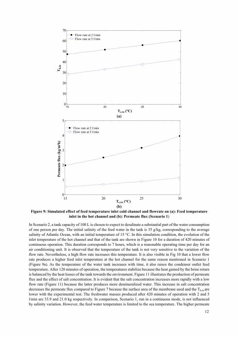
Figure 9 shows the effect of the seawater inlet temperature on the outlet temperature of the condenser of the cooling device and the permeate flux at a flow rate of 2 and 5 l/min. Different sea water temperatures (15 to 30 °C) were used to observe the behaviour of the coupled system studied. Figure 9a shows that the feed inlet temperature increases the inlet temperature in the hot channel. The condenser outlet temperatures are higher for the lower feed flow rate. This is due to the fact that the residence time of the feed solution is longer when the flow rate is lower. This results in an increase of the permeate flux (Figure 9b). The increase of the permeate flux is exponential with respect to the feed inlet temperature in the hot channel. This result can be seen in Figure 7 in the experimental validation work of the numerical model of the AGMD. Furthermore, the permeate flux is sensitive to the variation of the initial inlet temperature of the cold channel. The driving force behind the mass transfer in the AGMD process increases when the outlet temperature of the condenser (or feed inlet temperature in the hot channel) increases, which leads to an increase of the transmembrane vapour pressure gradient in accordance with the Antoine equation (equation 23). When the inlet temperature of the cold channel increases from 15 to 30 °C, the permeate flux is almost twice for a flow rate of 2 l/min. For a decrease of the flow rate of 5 to 2 l/min, there is an increase of 70.9 % with an inlet temperature of the cold channel of 30 °C.
12
15 20 25 300
10
20
30
40
50
60
70
Tc,in (°C)
T h,in
Flow rate at 2 l/minFlow rate at 5 l/min
(a)
15 20 25 300
1
2
3
4
5
Tc,in (°C)
Perm
eate
flux
(kg/
m²h
)
Flow rate at 2 l/minFlow rate at 5 l/min
(b)Figure 9: Simulated effect of feed temperature inlet cold channel and flowrate on (a): Feed temperature
inlet in the hot channel and (b): Permeate flux (Scenario 1)
In Scenario 2, a tank capacity of 100 L is chosen to expect to desalinate a substantial part of the water consumption of one person per day. The initial salinity of the feed water in the tank is 35 g/kg, corresponding to the average salinity of Atlantic Ocean, with an initial temperature of 15 °C. In this simulation condition, the evolution of the inlet temperature of the hot channel and that of the tank are shown in Figure 10 for a duration of 420 minutes of continuous operation. This duration corresponds to 7 hours, which is a reasonable operating time per day for an air conditioning unit. It is observed that the temperature of the tank is not very sensitive to the variation of the flow rate. Nevertheless, a high flow rate increases this temperature. It is also visible in Fig 10 that a lower flow rate produces a higher feed inlet temperature at the hot channel for the same reason mentioned in Scenario 1 (Figure 9a). As the temperature of the water tank increases with time, it also raises the condenser outlet feed temperature. After 120 minutes of operation, the temperatures stabilize because the heat gained by the brine return is balanced by the heat losses of the tank towards the environment. Figure 11 illustrates the production of permeate flux and the effect of salt concentration. It is evident that the salt concentration increases more rapidly with a low flow rate (Figure 11) because the latter produces more demineralized water. This increase in salt concentration decreases the permeate flux compared to Figure 7 because the surface area of the membrane used and the Th,in are lower with the experimental test. The freshwater masses produced after 420 minutes of operation with 2 and 5 l/min are 33.9 and 21.0 kg respectively. In comparison, Scenario 1, run in a continuous mode, is not influenced by salinity variation. However, the feed water temperature is limited to the sea temperature. The higher permeate

13
flux, being constant over time, enables to produce, in 420 minutes, only 27.9 and 8.0 kg with 2 and 5 l/min respectively. These values are obtained with a feed water temperature of 30 °C, which is lower than in Scenario 2.
0 60 120 180 240 300 360 4200
10
20
30
40
50
60
70
Time (min)
T h,in
,Tta
nk(°
C)
Th,in at 2 l/minTh;in at 5 l/minTtank at 2 l/minTtank at 5 l/min
Figure 10 Simulated effect of flow rates on tank and hot feed inlet temperatures (Scenario 2)
0 60 120 180 240 300 360 4200
1
2
3
4
5
6
0
10
20
30
40
50
60
Time (min)
Perm
eate
flux
(kg/
m²h
)
Permeate flux at 2 l/minPermeate flux at 5 l/min
Salin
ity(g
/kg)
Salinity at 2 l/minSalinity at 5 l/min
Figure 11: Simulated effect of flow rates on permeate flux and water tank salinity (Scenario 2)
4.2.3. Performance of the system
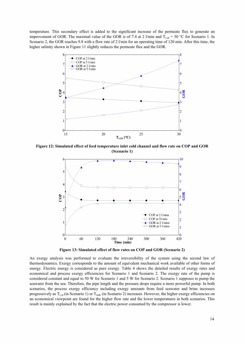
The COP, the GOR and the exergy efficiency are used to evaluate the performance of this system. The COP characterizes the performance of the air conditioner and the GOR, that of the MD. The COP of the air conditioner decreases considerably with the flow rate (Figures 12 and 13). For Scenario 1, an increase of the temperature of the seawater feed in the cold channel of the MD unit also reduces the COP as shown in Figure 12. In Scenario 2, the inlet temperature of the cold channel corresponds to the change in the temperature of the tank over time. As the temperature of the water tank stabilizes in 120 minutes of operation (Figure 10), this behaviour is constant with the COP (Figure 13). A decrease of the COP may penalize the functioning of the heat pump by increasing the power consumption of the compressor for the same cooling duty.
The GOR is also present in figures 12 and 13 respectively for Scenario 1 and Scenario 2. The GOR increases with the increase of Tc,in or Ttank and Th,in. When the temperature inlet of the cold channel increases, this results in a small decrease of the temperature difference, which means that it requires less heat to reach the required
14
temperature. This secondary effect is added to the significant increase of the permeate flux to generate an improvement of GOR. The maximal value of the GOR is of 7.4 at 2 l/min and Tc,in = 30 °C for Scenario 1. In Scenario 2, the GOR reaches 9.8 with a flow rate of 2 l/min for an operating time of 120 min. After this time, the higher salinity shown in Figure 11 slightly reduces the permeate flux and the GOR.
15 20 25 300
1
2
3
4
5
6
7
8
0
1
2
3
4
5
6
7
8
Tc,in (°C)
CO
PCOP at 2 l/minCOP at 5 l/minGOR at 2 l/minGOR at 5 l/min
GO
R
Figure 12: Simulated effect of feed temperature inlet cold channel and flow rate on COP and GOR (Scenario 1)
0 60 120 180 240 300 360 4200
1
2
3
4
5
6
0
1
2
3
4
5
6
7
8
9
10
Time (min)
CO
P
COP at 2 l/mimCOP at 5l/min
GO
R
GOR at 2 l/mimGOR at 5 l/mim
Figure 13: Simulated effect of flow rates on COP and GOR (Scenario 2)
An exergy analysis was performed to evaluate the irreversibility of the system using the second law of thermodynamics. Exergy corresponds to the amount of equivalent mechanical work available of other forms of energy. Electric energy is considered as pure exergy. Table 4 shows the detailed results of exergy rates and economical and process exergy efficiencies for Scenario 1 and Scenario 2. The exergy rate of the pump is considered constant and equal to 50 W for Scenario 1 and 5 W for Scenario 2. Scenario 1 supposes to pump the seawater from the sea. Therefore, the pipe length and the pressure drops require a more powerful pump. In both scenarios, the process exergy efficiency including exergy amounts from feed seawater and brine increases progressively as Tc,in (in Scenario 1) or Ttank (in Scenario 2) increases. However, the higher exergy efficiencies on an economical viewpoint are found for the higher flow rate and the lower temperatures in both scenarios. This result is mainly explained by the fact that the electric power consumed by the compressor is lower.

15
Table 4: Exergy analysis of individual components
5. Conclusion
A model of air conditioner operating with propane (R290) is used in this work for a coupling with an AGMD unit. The model results were compared with experimental data from an AGMD pilot plant. The long-term experiments show a constant salt rejection rate over 99.99% that validates the quality of the membrane and the process.
The effects of various operating parameters such as feed water temperature and flow rate on the permeate flux were studied and presented in this study. The analysis showed that the temperature outlet of the feed water is high when the residence time of the water is long inside the heat exchanger (condenser). It leads to a higher permeate flux. However, low flow rates and high cold channel inlet temperatures reduce the COP of the air conditioner but conversely, they increase the GOR in the two scenarios studied. In Scenario 1, the exergy efficiency is better with a high flow rate and low cold channel inlet temperature. In Scenario 2, increasing the temperature of the water tank seems to reduce the exergy efficiency for a long period of operation of the air conditioner. One advantage of Scenario 1 is that the salt concentration is constant and does not influence the permeate flux. In Scenario 2, the permeate flux decreases over time by the salt concentration in the water tank. This Scenario 2 can be improved in the future by reducing as much as possible the temperature of the tank.
The set of results presented here is interesting as being a first assessment of design parameters for an MD unit system coupled to an air conditioner. It confirms that the two scenarios can be envisaged for either coastal buildings or remote areas.
Nomenclature
A: surface area [m2]Bw: mass transfer coefficient [kg/m2·h·Pa]Cp: thermal capacity [J/kg·K]Dva: thermal diffusivity of water vapour in air [m2/s]dh: hydraulic diameter [m]e: specific exergy [J/kg]
: exergy rate [W]Exhc: convective heat transfer coefficient [W/m2·K]h: specific enthalpy [J/kg]HP: heat pumpJ: flux [kg/m2·s]k: thermal conductivity [W/m·K]L: module length [m]
: mass flow rate [kg/s]mNu: Nusselt number [-]P: pressure [Pa]
Scenario Flow rate [l/min]
Tc,in , Ttank[°C]
𝐄𝐱𝐞𝐥𝐞𝐜[kW]
𝐄𝐱𝐭𝐡[kW]
𝐄𝐱𝐬𝐰,𝐨𝐮𝐭[kW]
𝐄𝐱𝐰,𝐨𝐮𝐭[kW]
𝐄𝐱𝐬𝐰,𝐢𝐧[kW]
𝛈𝐞𝐱,𝐞𝐜𝐨[%]
𝛈𝐞𝐱,𝐩𝐫𝐨[%]
15 0.797 0.248 0.008 0.034 0.006 30.0 33.720 0.822 0.244 0.000 0.063 0.006 28.7 35.925 0.847 0.238 0.004 0.099 0.025 29.3 40.22
30 0.871 0.232 0.020 0.142 0.052 30.8 45.315 0.596 0.251 0.019 0.006 0.003 39.3 39.020 0.632 0.255 0.000 0.038 0.001 37.4 43.025 0.668 0.256 0.011 0.095 0.006 36.5 49.0
1
5
30 0.704 0.256 0.052 0.176 0.013 35.8 55.315.0 0.797 0.248 0.008 0.034 0.006 31.7 35.633.8 0.889 0.227 0.040 0.180 0.081 34.4 52.136.0 0.899 0.223 0.054 0.203 0.100 35.8 54.92
36.2 0.900 0.223 0.067 0.219 0.097 35.3 55.415.0 0.596 0.251 0.019 0.006 0.003 42.2 41.935.6 0.743 0.254 0.129 0.293 0.026 37.5 65.538.2 0.761 0.253 0.177 0.359 0.035 37.5 68.4
2
5
38.6 0.764 0.253 0.185 0.369 0.035 37.4 68.8

16
Pr: Prandtl number [-]: thermal flux [W/m2]φ: thermal capacity [W]Φ
Re: Reynolds number [-]R: thermal resistance [m²·K/W] R*: Gas constant [J/K·mol]R290: propane s: specific entropy [J/kg·K]S: salinity [g/kg]T: temperature [°C]t: time [s]
: (swept) volume [m3/s]𝑉U: heat transfer coefficient [W/m2·K]
: power [W]𝑊X: mole fraction [-]
Greek letters : activity coefficient [-]𝛼: water fraction [-]𝛽: thickness [m]𝛿: porosity [-]ε: efficiency [-]𝜂: electric conductivity [S/m]κ
µ: dynamic viscosity [kg/m·s]: density [kg/m3]𝜌: compression ratio [-]σ: tortuosity [-]τ
Subscripts 0: reference statea: airag: air gapc: coldcd: condenser ch: chemicalelec: electricev: evaporator ex: exergyf: feed h: hothm: hot fluid - membrane interfaceHX: exchanger heat in: inletis: isentropicm: membranema: membrane - air gap interfaceNaCl: sodium chlorideout: outlet p: permeatepc: cold fluid - plate interfacepp: temperature at permeate - plate interfacer: refrigerants: spacerso: sourcesw: seawaterth: thermalv: vapourvs: void in the spacerw: water

17
Acknowledgements
The authors would like to acknowledge the financial supports of this project by Région Bretagne and Fondation de la Banque Populaire de l’Ouest.
References
[1] Website of the French refrigeration association: www.aff.fr[2] HLPE, L’eau, enjeu pour la sécurité alimentaire mondiale. Rapport du Groupe d’experts de haut niveau sur la
sécurité alimentaire et la nutrition du Comité de la sécurité alimentaire mondiale, Rome 2015[3] P. Byrne, L. Fournaison, A. Delahaye, Y. Ait Oumeziane, L. Serres, P. Loulergue, A. Szymczyk, D. Mugnier,
J.-L. Malaval, R. Bourdais, H. Gueguen, O. Sow, J. Orfi, T. Mare. A review on the coupling of cooling, desalination and solar photovoltaic systems. Renewable and Sustainable Energy Reviews 47 (2015) 703–717
[4] P. Byrne, Y. Ait Oumeziane, L. Serres, J. Miriel, Numerical Study of a membrane distillation unit for desalination coupled to a heat pump, Applied Mechanics and Materials 819 (2016) 152-159
[5] R. Gonzalez-Bravo, N. A. Elsayed, J. M.Ponce-Ortega, F. N_Apoles-Rivera, M. M. El-Halwagi, Optimal design of thermal membrane distillation systems with heat integration with process plants, Applied Thermal Engineering 75 (2015) 154 – 166
[6] C. Charcosset, A review of membrane processes and renewable energies for desalination, Desalination 245 (2009) 214-231
[7] E. Drioli, Y. Wu and V. Calabro, Membrane distillation in the treatment of aqueous solutions, Journal of Membrane Science, 33 (1987) 277-284
[8] P. Wang, T.-S. Chung, Recent advances in membrane distillation processes: Membrane development, configuration design and application exploring, Journal of Membrane Science 474 (2015) 39 – 56
[9] R. Tian, H. Gao, X.H. Yang, S.Y. Yan, S. Li. A new enhancement technique on air gap membrane distillation, Desalination 332 (2014) 52-59
[10] E. K. Summers, V J.H. Lienhard, Experimental study of thermal performance in air gap membrane distillation systems, including the direct solar heating of membranes, Desalination 330 (2013) 300-311.
[11] M.A.E.-R. Abu-Zeid, Y. Zhang, H. Dong, L. Zhang, H.-L. Chen, L. Hou, A comprehensive review of vacuum membrane distillation technique, Desalination 356 (2015) 1–14
[12] S. Klein, Engineering Equation Solver, Version 10.200-3D, ©1992-2017[13] R. Ghoubali, P. Byrne, F. Bazantay, Simulation study of heat pumps for simultaneous heating and cooling
coupled to buildings. Energy and Buildings 72 (2014) 141–149[14] American Society of Heating, Refrigerating and Air Conditioning Engineers, ASHRAE Handbook,
Fundamentals, SI Edition (1989)[15] J. Navarro-Esbri, F. Moles, B. Peris, A. Barragan-Cervera, M. Mendoza-Miranda, A. Mota-Babiloni, J.M.
Belman, Shell-and-tube evaporator model performance with different two-phase flow heat transfer correlations. Experimental analysis using R134a and R1234yf, Applied Thermal Engineering 62 (2014) 80–89
[16] B. L. Pangarkar, S. K. Deshmukh, Theoretical and experimental analysis of multi-effect air gap membrane distillation process (ME-AGMD), Journal of Environmental Chemical Engineering 3 (2015) 2127–2135.
[17] R. Aryapratama, H. Koo, S. Jeong, S. Lee, Performance evaluation of hollow fiber air gap membrane distillation module with multiple cooling channels, Desalination 385 (2016) 58–68
[18] M. Khayet, Membranes and theoretical modeling of membrane distillation: A review, Advances in Colloid and Interface Science 164 (2011) 56–88
[19] J. Phattaranawik, R. Jiraratananon, A.G. Fane, C. Halim, Mass flux enhancement using spacer filled channels in direct contact membrane distillation, Journal of Membrane Science 187 (2001) 193–201
[20] M. Essalhi, M. Khayet, Application of a porous composite hydrophobic/hydrophilic membrane in desalination by air gap and liquid gap membrane distillation: A comparative study, Separation and Purification Technology 133 (2014) 176–186
[21] A. Khalifa, H. Ahmad, M. Antar, T. Laoui, M. Khayet, Experimental and theoretical investigations on water desalination using direct contact membrane distillation, Desalination 404 (2017) 22–34
[22] F. Macedonio, E. Drioli, An exergetic analysis of a membrane desalination system, Desalination 261 (2010) 293–299