Embed Size (px)
Citation preview
25
Designing evacuation routes with GeoGebra
Ph.D. Raúl M. Falcón School of Building Engineering. University of Seville, Spain.
Ángela Moreno Occupational Safety and HealthTechnician. SPM. Spain.
Ph.D. Ricardo Ríos I.E.S. Julio Verne, Seville, Spain.
ABSTRACT: We expose in this paper how the command ShortestDistance can be
used in GeoGebra to design evacuation routes in buildings in a dynamic and
interactive way. For those cases in which a legal regulation or procedure compels
specific requirements in the design, we also indicate how to make use of JavaScript in
order to implement a more general version of Dijkstra’s algorithm that makes possible
to deal with such specifications.
KEYWORDS: Evacuation route, Graph Theory, Dijkstra’s algorithm.
1 Introduction Nowadays, the importance of designing optimal evacuation routes in public and private
buildings is unquestionable due to the fact that they guarantee, with a very high
probability, the safe evacuation of all their occupants in case of any kind of emergency. In
the case of buildings like schools, hospitals or hotels, all these routes have to be clearly
visible to everybody and, because of that, it is usual or even mandatory to post evacuation
maps in all their rooms and corridors. The problem of these maps is that they are usually
fixed and static and they could point exactly at the cause of the emergency, like the seat of
a fire, for instance. In order to avoid these cases, it is interesting to have dynamic screens
or LED lamps that could show in real time which is exactly the evacuation route that must
be follow the person who is watching them. Keeping this idea in mind, we expose in this
paper how to use GeoGebra in order to design a dynamic evacuation map that make
possible a fast update of the evacuation routes of a building in case of being necessary.
The paper is organized as follows. In Section 2 we introduce the shortest path
problem in Graph theory and expose how the command ShortestDistance, which is
implemented by defect in GeoGebra, can be used to solve this problem. We focus
specifically on the creation of a template in GeoGebra that makes possible to design a
dynamic and interactive evacuation map of a building whose plan has been previously
inserted in the worksheet. In Section 3 we make use of JavaScript in order to implement in
GeoGebra the Dijkstra’s algorithm, which is commonly used to solve the shortest path
problem for any connected and weighted graphs with non-negative weights. This
implementation makes possible to deal with legal regulations or procedures that compel
specific requirements in the design of evacuation routes.
26
2 The shortest path problem We start with some basic results on Graph theory that are used throughout the paper. For
more details on this topic we refer to the monograph of Gross and Yellen [GY04].
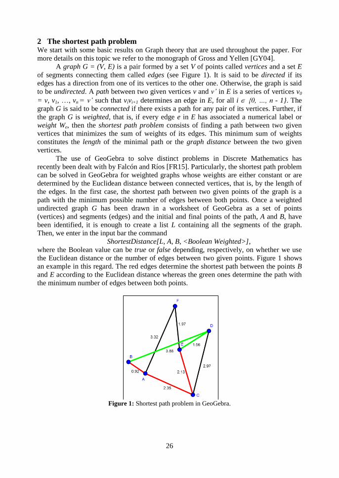
A graph G = (V, E) is a pair formed by a set V of points called vertices and a set E
of segments connecting them called edges (see Figure 1). It is said to be directed if its
edges has a direction from one of its vertices to the other one. Otherwise, the graph is said
to be undirected. A path between two given vertices v and v’ in E is a series of vertices v0
= v, v1, …, vn = v’ such that vivi+1 determines an edge in E, for all i {0, …, n - 1}. The
graph G is said to be connected if there exists a path for any pair of its vertices. Further, if
the graph G is weighted, that is, if every edge e in E has associated a numerical label or
weight We, then the shortest path problem consists of finding a path between two given
vertices that minimizes the sum of weights of its edges. This minimum sum of weights
constitutes the length of the minimal path or the graph distance between the two given
vertices.
The use of GeoGebra to solve distinct problems in Discrete Mathematics has
recently been dealt with by Falcón and Ríos [FR15]. Particularly, the shortest path problem
can be solved in GeoGebra for weighted graphs whose weights are either constant or are
determined by the Euclidean distance between connected vertices, that is, by the length of
the edges. In the first case, the shortest path between two given points of the graph is a
path with the minimum possible number of edges between both points. Once a weighted
undirected graph G has been drawn in a worksheet of GeoGebra as a set of points
(vertices) and segments (edges) and the initial and final points of the path, A and B, have
been identified, it is enough to create a list L containing all the segments of the graph.
Then, we enter in the input bar the command
ShortestDistance[L, A, B, <Boolean Weighted>],
where the Boolean value can be true or false depending, respectively, on whether we use
the Euclidean distance or the number of edges between two given points. Figure 1 shows
an example in this regard. The red edges determine the shortest path between the points B
and E according to the Euclidean distance whereas the green ones determine the path with
the minimum number of edges between both points.
Figure 1: Shortest path problem in GeoGebra.

27
The command ShortestDistance together with the dynamical structure of the graphics view
of Geogebra constitutes an especially useful tool to design dynamic and interactive
evacuation maps. In this regard, let us suppose that we are interested in designing an
evacuation map of the building whose plan is shown in Figure 2. It represents the ground
floor of the School of Building Engineering at the University of Seville, in which we can
observe the existence of three emergency exit doors. This map has conveniently been
inserted in the graphic view of GeoGebra in such a way that the image respects the real
scale. In this case, the real size of the plan is 720 x 740 m2.
Figure 2: Plan of the first ground of a school.
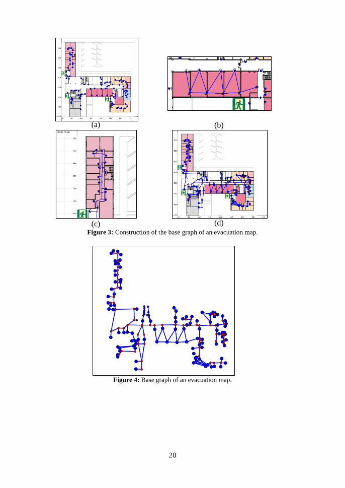
In order to design our evacuation map in GeoGebra, it is required to determine a
graph that represents the distribution of rooms, corridors and stairs. To this end we draw a
series of points and edges by following the next sequential order:
We draw a point for each door or stair in the plan (see Figure 3.a). The points
related to the emergency exit doors are called Exit1, Exit2 and Exit3.
We draw an edge for each pair of such points that are related to distinct doors in
a same room (see Figure 3.b).
In front of each door and stair, in the middle of corridors, we draw a point
connected by an edge with the point of the corresponding door or stair. Adjacent
points in the corridor are also connected with an edge (see Figure 3.c).
The resulting graph (see Figure 3.d and Figure 4) is called the base graph of the
evacuation map. Once this graph is constructed, we click on the tool Create List in the
Toolbar of GeoGebra and we create the list L of edges that will be used as argument of the
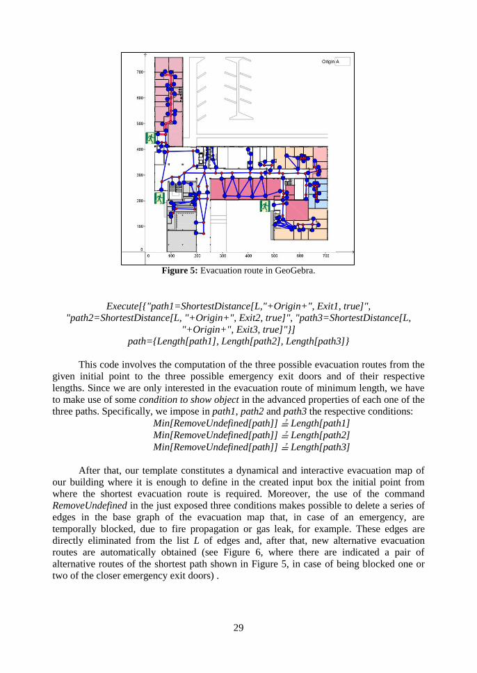
command ShortestDistance. After that, we define in the input bar the text Origin = “A”,
which we hide immediately after from the graphics view and for which we create a related
input box (see Figure 5). In the On Update tab of the Scripting tab of the input box, we
write the next code in GeoGebra script:
28
(a)
(b)
(c)
(d)
Figure 3: Construction of the base graph of an evacuation map.
Figure 4: Base graph of an evacuation map.
29
Figure 5: Evacuation route in GeoGebra.
Execute[{"path1=ShortestDistance[L,"+Origin+", Exit1, true]",
"path2=ShortestDistance[L, "+Origin+", Exit2, true]", "path3=ShortestDistance[L,
"+Origin+", Exit3, true]"}]
path={Length[path1], Length[path2], Length[path3]}
This code involves the computation of the three possible evacuation routes from the
given initial point to the three possible emergency exit doors and of their respective
lengths. Since we are only interested in the evacuation route of minimum length, we have
to make use of some condition to show object in the advanced properties of each one of the
three paths. Specifically, we impose in path1, path2 and path3 the respective conditions:
Min[RemoveUndefined[path]] ≟ Length[path1]
Min[RemoveUndefined[path]] ≟ Length[path2]
Min[RemoveUndefined[path]] ≟ Length[path3]
After that, our template constitutes a dynamical and interactive evacuation map of
our building where it is enough to define in the created input box the initial point from
where the shortest evacuation route is required. Moreover, the use of the command
RemoveUndefined in the just exposed three conditions makes possible to delete a series of
edges in the base graph of the evacuation map that, in case of an emergency, are
temporally blocked, due to fire propagation or gas leak, for example. These edges are
directly eliminated from the list L of edges and, after that, new alternative evacuation
routes are automatically obtained (see Figure 6, where there are indicated a pair of
alternative routes of the shortest path shown in Figure 5, in case of being blocked one or
two of the closer emergency exit doors) .
30
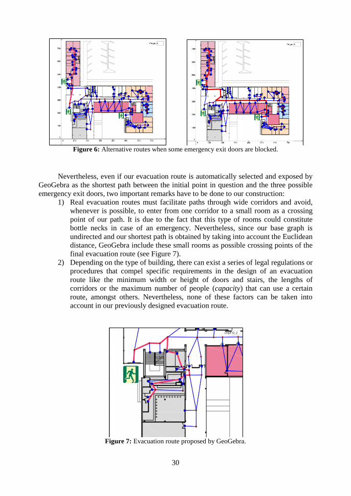
Figure 6: Alternative routes when some emergency exit doors are blocked.
Nevertheless, even if our evacuation route is automatically selected and exposed by
GeoGebra as the shortest path between the initial point in question and the three possible
emergency exit doors, two important remarks have to be done to our construction:
1) Real evacuation routes must facilitate paths through wide corridors and avoid,
whenever is possible, to enter from one corridor to a small room as a crossing
point of our path. It is due to the fact that this type of rooms could constitute
bottle necks in case of an emergency. Nevertheless, since our base graph is
undirected and our shortest path is obtained by taking into account the Euclidean
distance, GeoGebra include these small rooms as possible crossing points of the
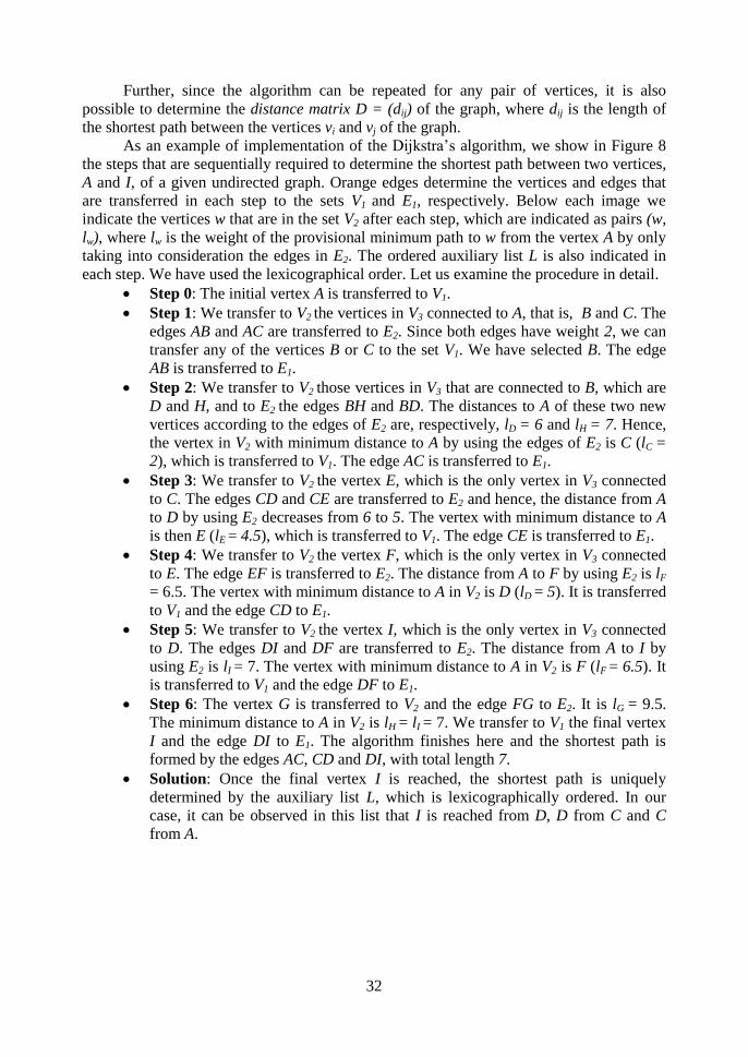
final evacuation route (see Figure 7).
2) Depending on the type of building, there can exist a series of legal regulations or
procedures that compel specific requirements in the design of an evacuation
route like the minimum width or height of doors and stairs, the lengths of
corridors or the maximum number of people (capacity) that can use a certain
route, amongst others. Nevertheless, none of these factors can be taken into
account in our previously designed evacuation route.
Figure 7: Evacuation route proposed by GeoGebra.
31
It is therefore necessary to generalize our construction in order to deal with more
realistic evacuation routes. To this end, we propose in the next section to make use of
Javascript in order to implement the Dijkstra’s algorithm in GeoGebra.
3 The Dijkstra’s algorithm In 1959, Edsger W. Dijkstra [Dij59] established an algorithm that solves the shortest path
problem for connected and weighted graphs with non-negative weights. These graphs can
be directed or undirected. In the course of the algorithm, given a weighted graph G = (V,
E) and the initial and final vertices, v and v’, of the path, Dijkstra subdivides the set of
vertices V into three sets:
The set V1 of vertices w for which the path of minimum length from v is known.
The set V2 of vertices in V– V1 that are connected by one edge to at least one
vertex of V1. If the graph is directed, then this edge must be oriented from the
vertex in V1 to the vertex in V2.
The set V3 formed by the rest of vertices.
Dijkstra also subdivides the set of edges E in other three sets:
The set E1 of edges in the minimal paths from v to the vertices of V1.
The set E2 of edges in E– E1 that connect vertices of V1 and V2.
The set E3 formed by the rest of edges.
At the beginning of the algorithm, all the vertices are in V3 and all the edges are in
E3. The vertex v is then the first vertex to be included in V1. At each step of the algorithm,
it is considered all the edges e that connect the last vertex w included in V1 with vertices w’
in V2 V3.
If the vertex w’ is in V3, then it is added to V2 and the edge e is added to E2. The
path of minimum length lw between v and w together with the edge e of weight
We determines a provisional path between v and w’ of length lw’ = lw + We.
If the vertex w’ is already in V2, then there exists exactly one edge e’ in E2 that
connects w’ with a vertex w’’ in V1 so that the path of minimum length lw’’
between v and w’’ together with the edge e’ of weight We’ determines a
provisional path of minimum length lw’ = lw’’ + We’. If lw’ ≤ lw + We, then the
edge e is rejected. Otherwise, the edge e replaces the edge e’ in V2.
After that, the vertex in V2 with the shortest provisional path from v and its related
edge in E2 are respectively transferred to V1 and E1, and the procedure is then repeated for
this new vertex in V1. The algorithm finishes when the final vertex v’ is transferred to V1.
In practice, the n vertices of the graph are initially ordered and labeled as v1,…, vn.
An auxiliary ordered list L of cardinality n, initialized as {0,…,0}, can then be defined in
the course of the algorithm in such a way that its ith element is the immediately previous
vertex through which any shortest path starting in v has to pass to get the vertex vi. It
coincides with the second vertex related to the edge that is transferred to E1 at the same
time that vi is transferred to V1. Once the algorithm finishes, this list determines all the
previous vertices through which the shortest path from v to v’ has to pass.
32
Further, since the algorithm can be repeated for any pair of vertices, it is also
possible to determine the distance matrix D = (dij) of the graph, where dij is the length of
the shortest path between the vertices vi and vj of the graph.
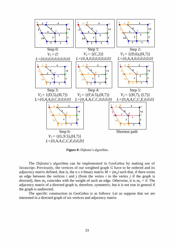
As an example of implementation of the Dijkstra’s algorithm, we show in Figure 8
the steps that are sequentially required to determine the shortest path between two vertices,
A and I, of a given undirected graph. Orange edges determine the vertices and edges that
are transferred in each step to the sets V1 and E1, respectively. Below each image we
indicate the vertices w that are in the set V2 after each step, which are indicated as pairs (w,
lw), where lw is the weight of the provisional minimum path to w from the vertex A by only
taking into consideration the edges in E2. The ordered auxiliary list L is also indicated in
each step. We have used the lexicographical order. Let us examine the procedure in detail.
Step 0: The initial vertex A is transferred to V1.
Step 1: We transfer to V2 the vertices in V3 connected to A, that is, B and C. The
edges AB and AC are transferred to E2. Since both edges have weight 2, we can
transfer any of the vertices B or C to the set V1. We have selected B. The edge
AB is transferred to E1.
Step 2: We transfer to V2 those vertices in V3 that are connected to B, which are
D and H, and to E2 the edges BH and BD. The distances to A of these two new
vertices according to the edges of E2 are, respectively, lD = 6 and lH = 7. Hence,
the vertex in V2 with minimum distance to A by using the edges of E2 is C (lC =
2), which is transferred to V1. The edge AC is transferred to E1.
Step 3: We transfer to V2 the vertex E, which is the only vertex in V3 connected
to C. The edges CD and CE are transferred to E2 and hence, the distance from A
to D by using E2 decreases from 6 to 5. The vertex with minimum distance to A
is then E (lE = 4.5), which is transferred to V1. The edge CE is transferred to E1.
Step 4: We transfer to V2 the vertex F, which is the only vertex in V3 connected
to E. The edge EF is transferred to E2. The distance from A to F by using E2 is lF
= 6.5. The vertex with minimum distance to A in V2 is D (lD = 5). It is transferred
to V1 and the edge CD to E1.
Step 5: We transfer to V2 the vertex I, which is the only vertex in V3 connected
to D. The edges DI and DF are transferred to E2. The distance from A to I by
using E2 is lI = 7. The vertex with minimum distance to A in V2 is F (lF = 6.5). It
is transferred to V1 and the edge DF to E1.
Step 6: The vertex G is transferred to V2 and the edge FG to E2. It is lG = 9.5.
The minimum distance to A in V2 is lH = lI = 7. We transfer to V1 the final vertex
I and the edge DI to E1. The algorithm finishes here and the shortest path is
formed by the edges AC, CD and DI, with total length 7.
Solution: Once the final vertex I is reached, the shortest path is uniquely
determined by the auxiliary list L, which is lexicographically ordered. In our
case, it can be observed in this list that I is reached from D, D from C and C
from A.
33
Step 0:
V2 =
L={0,0,0,0,0,0,0,0,0}
Step 1:
V2 = {(C,2)}
L={0,A,0,0,0,0,0,0,0}
Step 2:
V2 = {(D,6),(H,7)}
L={0,A,A,0,0,0,0,0,0}
Step 3:
V2 = {(D,5),(H,7)}
L={0,A,A,0,C,0,0,0,0}
Step 4:
V2 = {(F,6.5),(H,7)}
L={0,A,A,C,C,0,0,0,0}
Step 5:
V2 = {(H,7), (I,7)}
L={0,A,A,C,C,E,0,0,0}
Step 6:
V2 = {(G,9.5),(H,7)}
L={0,A,A,C,C,E,0,0,D}
Shortest path
Figure 8: Dijkstra’s algorithm.
The Dijkstra’s algorithm can be implemented in GeoGebra by making use of
Javascript. Previously, the vertices of our weighted graph G have to be ordered and its
adjacency matrix defined, that is, the n x n binary matrix M = (mij) such that, if there exists
an edge between the vertices i and j (from the vertex i to the vertex j if the graph is
directed), then mij coincides with the weight of such an edge. Otherwise, it is mij = 0. The
adjacency matrix of a directed graph is, therefore, symmetric, but it is not true in general if
the graph is undirected.
The specific construction in GeoGebra is as follows: Let us suppose that we are
interested in a directed graph of six vertices and adjacency matrix
34
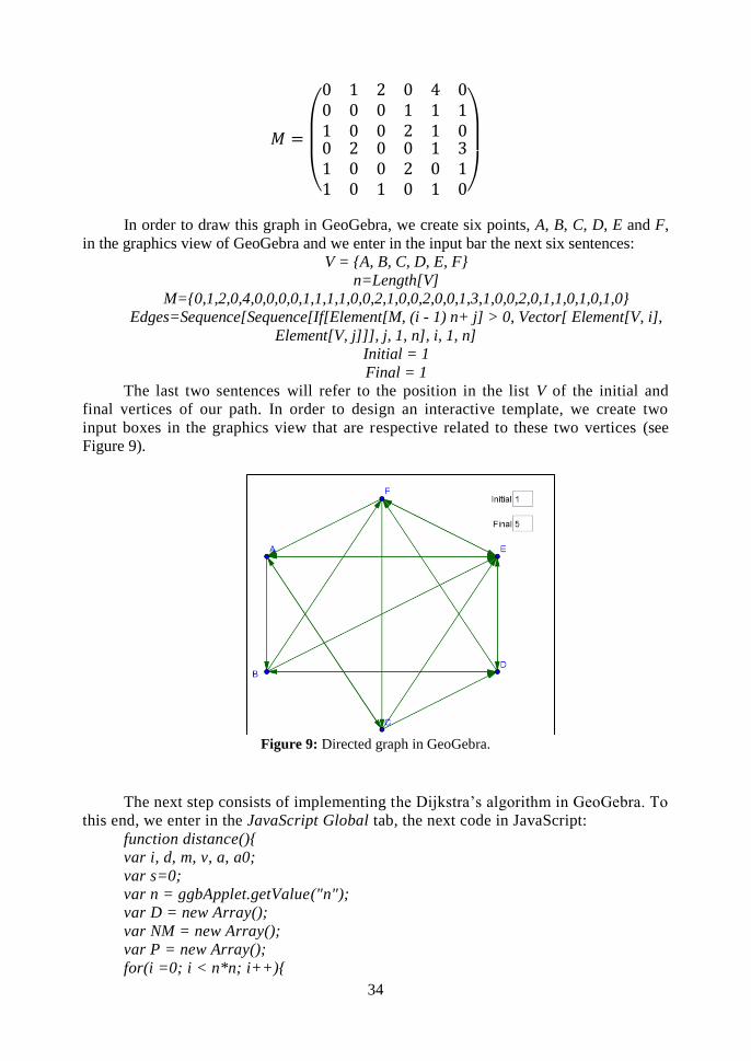
In order to draw this graph in GeoGebra, we create six points, A, B, C, D, E and F,
in the graphics view of GeoGebra and we enter in the input bar the next six sentences:
V = {A, B, C, D, E, F}
n=Length[V]
M={0,1,2,0,4,0,0,0,0,1,1,1,1,0,0,2,1,0,0,2,0,0,1,3,1,0,0,2,0,1,1,0,1,0,1,0}
Edges=Sequence[Sequence[If[Element[M, (i - 1) n+ j] > 0, Vector[ Element[V, i],
Element[V, j]]], j, 1, n], i, 1, n]
Initial = 1
Final = 1
The last two sentences will refer to the position in the list V of the initial and
final vertices of our path. In order to design an interactive template, we create two
input boxes in the graphics view that are respective related to these two vertices (see
Figure 9).
Figure 9: Directed graph in GeoGebra.
The next step consists of implementing the Dijkstra’s algorithm in GeoGebra. To
this end, we enter in the JavaScript Global tab, the next code in JavaScript:
function distance(){
var i, d, m, v, a, a0;
var s=0;
var n = ggbApplet.getValue("n");
var D = new Array();
var NM = new Array();
var P = new Array();
for(i =0; i < n*n; i++){
35
D[i] = 100;}
for(a0 =1; a0 < n+1; a0++){
for(i =0;i<n;i++){
NM[i]=0;
P[i]=-1;
D[n*n+(a0-1)*n+i]=-1;}
a=a0;
D[(a0-1)*n+a-1]=0;
NM[a-1]=1;
while(a!=0){
for(i =0;i<n;i++){
m=ggbApplet.getListValue("M",(a-1)*n +i+1);
if (NM[i]==0 & m!=0 & D[(a0-1)*n+i]>D[(a0-1)*n+a-1]+m){
D[(a0-1)*n+i]=D[(a0-1)*n+a-1]+m;
P[i]=a;
D[n*n+(a0-1)*n+i]=a;}}
d=100;
for(i=0;i<n;i++){
if (NM[i]==0){
if (s==0){
s=i;
d=D[(a0-1)*n+i];}
else{
if (D[(a0-1)*n+i]<d){
d=D[(a0-1)*n+i];
s=i;}}}}
if (d==100){
v=0;}
else{
v=s;}
if (v==0){
a=0;}
else{
NM[v]=1;
a=v+1;}}}
return(D);}
The output of this function is an array D of cardinality 2n2, such that its n
2 first
elements determine the distances among the vertices of the graph. These first elements
are initialized to 100, which would correspond to the maximum possible weight of the
graph in question. Depending on the graph, this initial value can conveniently be
increased. Further, the n2 last elements of the array D determine the list of previous
vertices in any shortest path from a given initial vertex.
Since D is not yet an explicit object in GeoGebra, we enter the next code in
JavaScript in the On Update tab of the Scripting properties of the numbers Initial and
Final:
ggbApplet.evalCommand("d={"+distance()+"}");
We can then press F9 or to introduce a number in any of the two input boxes of
our template to define automatically an auxiliary list d with all the 2n2
elements of the
36
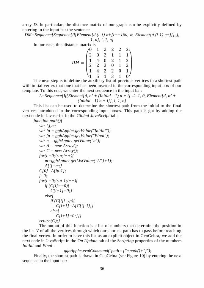
array D. In particular, the distance matrix of our graph can be explicitly defined by
entering in the input bar the sentence
DM=Sequence[Sequence[If[Element[d,(i-1) n+j]==100, ∞, Element[d,(i-1) n+j]], j,
1, n], i, 1, n]
In our case, this distance matrix is
The next step is to define the auxiliary list of previous vertices in a shortest path
with initial vertex that one that has been inserted in the corresponding input box of our
template. To this end, we enter the next sequence in the input bar:
L=Sequence[If[Element[d, n² + (Initial - 1) n + i] ≟ -1, 0, Element[d, n² +
(Initial - 1) n + i]], i, 1, n]
This list can be used to determine the shortest path from the initial to the final
vertices introduced in the corresponding input boxes. This path is got by adding the
next code in Javascript in the Global JavaScript tab:
function path(){
var i,j,m;
var ip = ggbApplet.getValue("Initial");
var fp = ggbApplet.getValue("Final");
var n = ggbApplet.getValue("n");
var A = new Array();
var C = new Array();
for(i =0;i<n;i++){
m=ggbApplet.getListValue("L",i+1);
A[i]=m;}
C[0]=A[fp-1];
j=0;
for(i =0;i<n-1;i++){
if (C[i]==0){
C[i+1]=0;}
else{
if (C[i]!=ip){
C[i+1]=A[C[i]-1];}
else{
C[i+1]=0;}}}
return(C);}
The output of this function is a list of numbers that determine the position in
the list V of all the vertices through which our shortest path has to pass before reaching
the final vertex. In order to have this list as an explicit object in GeoGebra, we add the
next code in JavaScript in the On Update tab of the Scripting properties of the numbers
Initial and Final:
ggbApplet.evalCommand("path= {"+path()+"}");
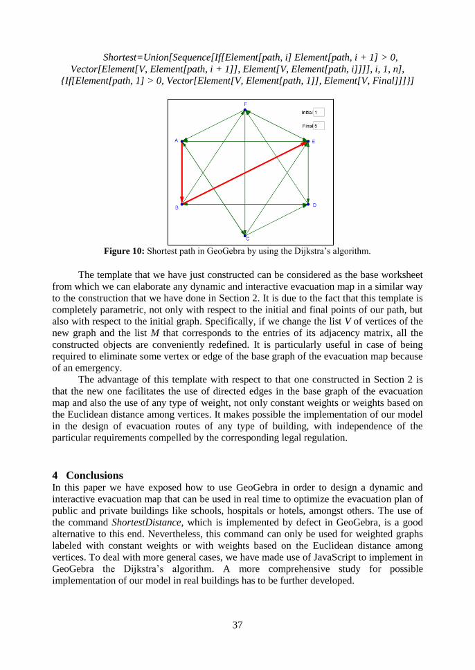
Finally, the shortest path is drawn in GeoGebra (see Figure 10) by entering the next
sequence in the input bar:
37
Shortest=Union[Sequence[If[Element[path, i] Element[path, i + 1] > 0,
Vector[Element[V, Element[path, i + 1]], Element[V, Element[path, i]]]], i, 1, n],
{If[Element[path, 1] > 0, Vector[Element[V, Element[path, 1]], Element[V, Final]]]}]
Figure 10: Shortest path in GeoGebra by using the Dijkstra’s algorithm.
The template that we have just constructed can be considered as the base worksheet
from which we can elaborate any dynamic and interactive evacuation map in a similar way
to the construction that we have done in Section 2. It is due to the fact that this template is
completely parametric, not only with respect to the initial and final points of our path, but
also with respect to the initial graph. Specifically, if we change the list V of vertices of the
new graph and the list M that corresponds to the entries of its adjacency matrix, all the
constructed objects are conveniently redefined. It is particularly useful in case of being
required to eliminate some vertex or edge of the base graph of the evacuation map because
of an emergency.
The advantage of this template with respect to that one constructed in Section 2 is
that the new one facilitates the use of directed edges in the base graph of the evacuation
map and also the use of any type of weight, not only constant weights or weights based on
the Euclidean distance among vertices. It makes possible the implementation of our model
in the design of evacuation routes of any type of building, with independence of the
particular requirements compelled by the corresponding legal regulation.
4 Conclusions In this paper we have exposed how to use GeoGebra in order to design a dynamic and
interactive evacuation map that can be used in real time to optimize the evacuation plan of
public and private buildings like schools, hospitals or hotels, amongst others. The use of
the command ShortestDistance, which is implemented by defect in GeoGebra, is a good
alternative to this end. Nevertheless, this command can only be used for weighted graphs
labeled with constant weights or with weights based on the Euclidean distance among
vertices. To deal with more general cases, we have made use of JavaScript to implement in
GeoGebra the Dijkstra’s algorithm. A more comprehensive study for possible
implementation of our model in real buildings has to be further developed.
38
References
[Dij59] E. W. Dijkstra – A note on two problems in connexion with graphs,
Numerische Mathematik, vol. 1: 269-271, 1959.
[FR15] R. M. Falcón, R. Ríos – The use of GeoGebra in Discrete Mathematics,
GeoGebra International Journal of Romania, Vol. 4 (1): 39-50, 2015.
[GY04] J. L. Gross, J. Yellen (eds.) – Handbook of graph theory, CRC Press, 2004.