Designing Ranking Systems for Hotels on Travel Search Engines by Mining

User-Generated and Crowd-Sourced Content1

Anindya Ghose, Panagiotis G. Ipeirotis, Beibei Li

Stern School of Business, New York University

(aghose, panos, bli)@stern.nyu.edu

Abstract

User-Generated Content (UGC) on social media platforms is changing the way consumers shop for

goods. However, current product search engines fail to effectively leverage information created across diverse social media platforms. Moreover, current ranking algorithms in these product search engines tend to induce consumers to focus on one single product characteristic dimension (e.g., price, star rating, etc). This largely ignores consumers’ multi-dimensional preferences for products. In this paper, we propose to generate a ranking system that recommends products providing the best value for money on an average. The key idea is that products that provide consumers with a higher surplus should be ranked higher on the screen in response to consumer queries. Our study is instantiated on a unique dataset of US hotel reservations over a 3-month period from Travelocity which is supplemented with data from various social media sources using techniques from text mining, image classification, social geo-tagging, human annotations and geo-mapping. We propose a random coefficient hybrid structural model, taking into consideration the two sources of consumer heterogeneity introduced by the different travel occasions and different hotel characteristics. Based on the estimates from the model, we infer the economic impact of various location and service characteristics of hotels. We then propose a new hotel ranking system based on the average utility gain that a consumer gets by staying in a particular hotel. By doing so, we can provide customers with the “best-value" hotels early on, and thereby improve the quality of local searches for such hotels. Our lab experiments in six major cities, using ranking comparisons from several thousand users, validate that our ranking system is superior to existing systems on several travel search engines. On a broader note, the objective of this paper is to illustrate how user-generated content (UGC) on the Internet can be mined and incorporated into a demand estimation model, and how UGC can be leveraged to generate a new ranking system in product search engines to improve the quality of choices available to consumers online. Our inter-disciplinary approach can provide insights for using text mining and image classification techniques in economics and marketing research.

1 We thank Susan Athey, Peter Fader, Brett Gordon, John Hauser, Francois Moreau, Aviv Nevo, Duncan Simester,

Minjae Song, Daniel Spulber, Catherine Tucker, and Hal Varian for extremely helpful comments that have

significantly improved the paper. We also thank participants at the 2011 Toulouse Conference on the Economics of

the Internet and Software, 2010 NBER IT Economics & Productivity Workshop, 2010 Workshop on Digital Business

Models, 2010 Marketing Science Conference, 2010 Searle Research Symposium on the Economics and Law of

Internet Search at NorthWestern University, Customer Insights Conference at Yale University, 2010 Statistical

Challenges in Ecommerce Research (SCECR) conference, 2009 Workshop on Information Technology and Systems

(WITS), 2009 Workshop on Economics and Information Systems and seminar participants at Columbia, Harvard,

George Mason, Georgia Tech, MIT, University of Maryland at College Park, Seoul National University, Temple

University, and University of Minnesota for helpful comments. Anindya Ghose and Panos Ipeirotis acknowledge the

financial support from National Science Foundation CAREER Awards IIS-0643847 and IIS-0643846, respectively.

Support was also provided through a MSI-Wharton Interactive Media Grant (WIMI) and a Microsoft Virtual Earth

Award. The authors thank Travelocity for providing the data and Uthaman Palaniappan for research assistance.

2

1. Introduction

As online social media and User-Generated Content (UGC) are increasing in popularity, consumers

today rely on a large variety of Internet-based sources prior to making a purchase. During the search

process, customers try to identify products that satisfy particular criteria, such as quality, availability, and

so on. Once they identify the candidates, customers would typically look at the price and determine if the

“real value” of that product matches the corresponding price. Hence, locating a product with the specific

desired characteristics, but without compromising on the value, becomes an important task.

However, although online product search engines have access to lots of UGC (not only on their own

site but also across other social media channels), they typically fail to effectively leverage and present such

product information, going beyond simple numerical ratings. Consequently, online product search is

constrained by consumer cognitive limitations. Moreover, existing ranking algorithms typically induce

consumers to only focus on one single product characteristic dimension (e.g., price, star rating, etc). This

largely ignores the multi-dimensional preferences and heterogeneity of consumers.. In this paper, we

propose a “utility-preserving” ranking strategy that aims at maximizing the expected utility gain for

consumers from a product purchase. Our approach is able to facilitate consumers’ economic decision

making process.

We instantiate our study by looking into the hotel industry. According to a study by ComScore, more

than 87% of customers rely on the online UGC to make purchase decision for hotels, higher than any other

product category2. This necessitates a better ranking mechanism on travel search engines that can

efficiently incorporate the publicly available, but latent knowledge within and across a large variety of

social media platforms. For this goal, we propose to build a system that ranks each hotel according to the

expected utility gain across the consumer population. The advantage of this system is that it uses consumer

utility theory to design a scalar utility score with which to rank hotels while incorporating all the

dimensions of hotel quality observed from diverse information sources. Currently, there are no established

measures that quantify the economic impact of various internal (service) and external (location)

characteristics on hotel demand. By analyzing information from online social media and UGC, we are able

to estimate the heterogeneous consumer preferences towards different hotel characteristics, and help

consumers quickly identify their best buy.

We use a unique dataset of hotel reservations from Travelocity.com. The dataset contains complete

information on transactions conducted over a 3-month period from 11/2008 to 1/2009 for 1497 hotels in the

United States (US). We have data on UGC from three sources: (i) user-generated hotel reviews from two

well-known travel search engines, Travelocity.com and TripAdvisor.com, (ii) social-geo tags generated by

users identifying different geographic attributes of hotels from Geonames.org, and (iii) user-contributed

opinions on the most important hotel characteristics using on-demand surveys and social annotations from

2 http://comscore.com, The Kelsey Group, October 2007.

3

users on Amazon Mechanical Turk (AMT).3 Moreover, since some location-based characteristics, such as

proximity to the beach, are not directly measurable based on UGC, we use image classification techniques

to infer such features from the satellite images of the area. These different data sources are then merged to

create one comprehensive dataset summarizing the location and service characteristics of all the hotels. Our

empirical modeling and analyses enables us to compute the “average utility gain” from a particular hotel

based on the estimation of price elasticities and average utilities. Our lab experiments in six major cities,

using 15,600 ranking comparisons from AMT, suggest that our ranking system is superior to the existing

benchmark systems.

Our work involves four steps:

i. Identify the important hotel location and service characteristics that influence hotel demand and

collect that data.

ii. Estimate how these hotel characteristics influence demand and quantify their marginal effects using

a structural model.

iii. Impute the expected utility from each hotel based on demand estimation and generate rankings

based on them

iv. Validate our ranking system by conducting lab experiments using AMT.

More specifically, in the first step, we determine the particular hotel characteristics that are most

valued by customers, and thus, influence the aggregate demand of the hotels. Beyond the directly

observable characteristics, such as the “number of stars,” provided by most third-party travel websites,

many users also tend to value location characteristics, such as proximity to the beach, or proximity to

downtown shopping areas. In our work, we incorporate satellite image classification techniques and use

both human and computer intelligence (in the form of social geo-tagging and text mining of reviews) to

infer these location features. In the second step, we use demand estimation techniques (BLP 1995, Berry

and Pakes 2007, Song 2011) and estimate the economic value associated with various location and service

characteristics. This enables us to quantitatively analyze how each feature influences demand and estimate

its importance relative to the other features. In the third step, after inferring the economic significance of

the location and service-based hotel characteristics, we incorporate them into designing a hotel ranking

system based on the expected utility gain from a given hotel. By doing so, we can provide customers with

the “best-value" hotels early on, thereby improving the quality of online hotel search compared to existing

systems. In the final step, we validate our proposed ranking system by conducting lab experiments with

3“Social annotation” is an annotation associated with a web resource (e.g., a web page, an online image, etc.). On a

social annotation system (e.g., the Amazon Mechanical Turk tool in our case), a user can add, modify or remove

information from the web resource without modifying the resource itself. The annotations can be thought of as a layer

on top of the existing resource, and this annotation layer is usually visible to other users who share the same

annotation system. In such cases, the web annotation tool is a type of social software tool.

4

users on the popular on-demand social annotation site, AMT, across six different cities. Our key results are

as follows.

i. Five location-based characteristics have a positive impact on hotel demand: “number of external

amenities,” “presence near a beach”, “presence near public transportation,” “presence near a highway,”

and “presence near a Downtown.” The textual content and style of reviews also demonstrate a

statistically significant association with demand. Reviews that are less complex, have words with fewer

syllables, and with fewer spelling errors have a positive influence on demand. Reviews with higher

number of characters and written using simple language are also positively associated with demand.

These results suggest that consumers can form an image about the quality of a hotel from the quality of

the user-generated reviews. Consumers prefer hotels with reviews that contain objective information

(such as factual descriptions of hotels) relative to subjective information, indicating that they do not

trust completely hotel-provided descriptions and prefer confirmation from third-parties. Consumers

also prefer to stay in hotels with reviews written in a “consistent objective style” rather than staying in

a hotel where the user reviews discuss more subjective aspects of the accommodation.

ii. We extend the basic model to examine interaction effects between travel purpose, price, and hotel

characteristics. Our results show that consumer preferences for location and service characteristics are

influenced by price and travel purpose. For instance, business travelers are the least price sensitive

while tourists are the most price sensitive. In addition, business travelers have the highest marginal

valuation for hotels located closer to a highway and having easy access to public transportation. In

contrast, romance travelers have the highest marginal valuation for hotels located closer to a beach and

those with a high service rating.

iii. A comparison of the model that conditions on the UGC variables with a model that does not shows that

the model with UGC variables outperformed the latter in both in- and out-of-sample analyses. We

conduct additional model fit comparisons and find that the model’s predictive power drops the most

when excluding all the location variables, followed by the service variables and then the UGC

variables. Moreover, within the set of UGC variables, we find that textual information (e.g., text

features, review subjectivity, and readability) has significantly higher impact than numerical

information on the model’s predictive power.

Our key contributions are as follows. First, we illustrate how user-generated content (UGC) from

multiple and diverse sources on the Internet can be mined towards examining the economic value of

different product attributes using a structural model of demand estimation. Customers today make their

decisions in an environment with the plethora of available data. It is possible that some consumers check

the characteristics of the hotel using tourist guides and mapping applications, or consult online review sites

to determine the quality of the hotel and its amenities. In order to replicate this decision-making

environment, we construct an exhaustive dataset, collecting information using a variety of data sources, and

5

a variety of methodologies such as text mining, on-demand annotations, and image classification. We

demonstrate the marginal contribution from different information sources by conducting model fit

comparisons between models that condition for one set of variables vs. others.

Second, our empirical estimates enable us to propose a new ranking system for hotel search based on

the computation of expected utility gain from each hotel. The proposed system ranks hotels based on the

computation of expected utility gain, which measures the “value” that a consumer gets from the transaction.

The key notion is that in response to a consumer search query, the system would recommend and rank

those hotels higher that provide a higher “value for money” by taking into account consumers’ multi-

dimensional preferences. Thus, our paper shows how UGC can be leveraged to generate a new ranking

system in product search engines to improve the quality of choices available to consumers online.

Finally, to evaluate the quality of our ranking technique, we conducted a user study toward which we

designed and executed several lab experiments on AMT across six different markets in the US. Using more

than 15,600 cumulative and 7,800 unique user responses for comparing different rankings, we show that

our proposed ranking performs significantly better than several baseline-ranking systems that are being

currently used by travel search engines. A post-experimental survey revealed users strongly preferred the

diversity of the retrieved results, given that our list consisted of a mix of hotels cutting across several price

and quality ranges. This indicates that customers prefer a list of hotels that each specializes in a variety of

characteristics, rather than a variety of hotels that each specializes in only one characteristic. Besides

providing consumers with direct economic gains, such a ranking system can lead to non-trivial reduction in

consumer search costs. Furthermore, by directing the customers to hotels that are better matches for their

interests, this can lead to increased usage of travel search engines.

The rest of the paper is organized as follows. Section 2 discusses related work and places our work in

the context of prior literature. Section 3 discusses the work related to the data preparation, including the

methods used to identify important hotel characteristics, the steps undertaken to conduct the surveys on

AMT to elicit user opinions, and the text mining techniques used to parse user-generated reviews. In

Sections 4 and 5, we provide an overview of our econometric approach, and discuss empirical results,

respectively. In Section 6, we discuss how one can apply our approach to design a real-world application,

such as a ranking system for hotel search. In Section 7, we conclude.

2. Prior Literature

Our paper draws from multiple streams of work. A key challenge is to bridge the gap between the

textual and qualitative nature of review content and the quantitative nature of discrete choice models. With

the rapid growth and popularity of the UGC on the Web, a new area of research applying text mining

technique to product reviews has emerged. The first stream of this research has focused on the sentiment

analysis of product reviews (Hu & Liu 2004, Pang & Lee 2004, Das & Chen 2007). This stimulated

6

additional research on identifying product features in which consumers expressed their opinions (Hu & Liu

2004, Scaffidi et al. 2007, Snyder & Barzilay 2007). The automated extraction of product attributes has

also received attention in the recent marketing literature (Lee & Bradlow 2007).

Meanwhile, the hypothesis that product reviews affect product sales has received strong support in

prior empirical studies (for example, Godes and Mayzlin 2004, Chevalier and Mayzlin 2006, Liu 2006,

Dellarocas et al. 2007, Duan et al. 2008, Forman et al. 2008, Moe 2009). However, these studies focus only

on numeric review ratings (e.g., the valence and volume of reviews) in their empirical analysis. Researchers

using only numeric ratings have to deal with issues like self-selection bias (Li and Hitt 2008) and bimodal

distribution of reviews (Hu et al. 2008). More importantly, the matching of consumers to hotels in

numerical rating systems is not random. A consumer only rates the hotel that she frequents (i.e. the one that

maximizes her utility). Consequently, the average star rating for each hotel need not reflect the population

average utility. Due to the above drawbacks, the average numerical star rating assigned to a product may

not convey a lot of information to a prospective buyer.

To the best of our knowledge, only a handful of empirical studies have formally tested whether the

textual information embedded in online user-generated content can have an economic impact. Ghose et al.

(2007) estimate the impact of buyer textual feedback on price premiums charged by sellers in online

second-hand markets. Eliashberg et al. (2007) combine natural-language processing techniques, and

statistical learning methods to forecast the return on investment for a movie, using shallow textual features

from movie scripts. Netzer et al. (2011) combine text mining and semantic network analysis to understand

the brand associative network and the implied market structure. Decker and Trusov (2010) use text mining

to estimate the relative effect of product attributes and brand names on the overall evaluation of the

products. None of these studies focus on estimating the impact of user-generated product reviews in

influencing product sales beyond the effect of numeric review ratings, which is one of the key research

objectives of this paper. The papers closest to this paper are Ghose and Ipeirotis (2011) and Archak et al.

(2011) who explore multiple aspects of review text to identify important text-based features and study their

impact on review helpfulness (Ghose and Ipeirotis 2011) and product sales (Ghose and Ipeirotis 2011,

Archak et al. 2011). However, these studies do not have data on actual product demand and they do not use

structural models. Nor do they examine the use of UGC in developing a ranking system for product search

in online markets.

Our work is related to models of demand estimation. One model that has made a significant

contribution to the field is the random coefficient logit model or BLP 1995 (Berry et al. 1995). Due to the

limitations of the product-level “taste shock” in logit models, a new model based on pure product

characteristics has been proposed recently (Berry and Pakes 2007). The pure characteristic model

(hereafter, PCM) differs from the BLP model in the sense that it does not contain the product-level “taste

shock.” It describes the consumer heterogeneity, purely based on their different tastes towards individual

product characteristics, without considerations on the tastes of certain products as a whole (i.e., brand

7

preference). However in reality, the product-level idiosyncratic “tastes” of different consumers do exist in

many markets. As pointed out in Song (2011), whether or not one should introduce the product-level “taste

shock” should depend on the context of the market. Keeping in mind the two levels of consumer

heterogeneity introduced by (1) different travel categories (i.e., family trip, romance, or business trip) and

(2) different hotel characteristics, we propose a random coefficient hybrid structural model to identify the

latent weight distribution that consumers assign to each hotel characteristic. The outcome of our analysis

enables us to compute the expected utility gain from each hotel and rank them accordingly on a travel

search engine.

Finally, our paper is related to the work in online recommender systems. By generating a novel

ranking approach for hotels, we aim to improve the recommendation strategy for travel search engines and

provide customers with the “best-value" hotels early on in the search process. In the marketing literature,

several model-based recommendation systems have been proposed to predict preferences for recommended

items (Ansari et al. 2000, Ying et al. 2005, Bodapati 2008). A more recent trend along this line is Adaptive

Personalization Systems (Ansari and Mela 2003, Rust and Chung 2006, Chung et al. 2009).

3. Data Description

Our dataset consisted of observations from 1479 hotels in the US. We collected data from various

sources to conduct our study. We had 3 months of hotel transaction data from Travelocity.com from

November 1, 2008 to January 31, 2009, which contained the average transaction price per room per night

and the total number of rooms sold per transaction.

Next, we discuss the data preparation work that is required. Our work leveraged three types of UGC

data:

On-demand user-contributed opinions through Amazon Mechanical Turk

Location description based on user-generated geo-tagging and image classification

Service description based on user-generated product reviews

We first discuss how we leverage Amazon Mechanical Turk to collect information on user preferences

for different hotel characteristics. Their responses suggest that these characteristics can be lumped into two

groups: location and service characteristics. Once we identify the set of consumer preferences, we use

other kinds of UGC to infer the external location characteristics, the internal service characteristics, and the

textual characteristics of hotel reviews that can influence consumer purchases. For a better understanding of

the variables in our setting, we present the data sources, definitions, and summary statistics of all variables

in Tables 1 and 2.

3.1 Identification of Hotel Characteristics using Amazon Mechanical Turk (AMT)

8

Our analysis first requires knowledge of those aspects of a hotel that are most important to consumers.

These factors determine the aggregate prices of the hotels. For our research, we wanted to avoid imposing

ourselves the features that we need to consider. Rather, we decided to rely on a survey of potential hotel

customers and ask them about the hotel aspects that are important for their purchasing decisions.

We do this through an online survey of users. In order to reach a wide demographic, we decided to

rely on the crowd-sourcing marketplace of Amazon Mechanical Turk (AMT). AMT is an online

marketplace, used to automate the execution of micro-tasks that require human intervention (i.e., cannot be

fully automated using data mining tools). Task requesters post simple micro-tasks, known as hits (human

intelligence tasks), in the marketplace. The marketplace provides proper control over the task execution,

such as validation of the submitted answers, or the ability to assign the same task to several different

workers. It also ensures the proper randomization of the assignments of tasks to workers within a single

task type. Each user receives a small monetary compensation for completing the task.

For our purposes, our main goal was to have a diversity of consumer opinions. Therefore, before using

AMT for our survey, we wanted to ensure that the participants are representative of the overall Internet

population. Towards this goal, we constructed a survey, asking AMT workers to give us information about

their place of origin and residence, gender, age, education attainment, income, marital status, household

size, and number of children. We also asked them about the time that they spend every week on AMT, the

amount of work that they complete, the payment they receive, and their reasons for participating on AMT.

To ensure that the results were not accidental, we conducted the survey multiple times, once every month.

The results of the surveys were consistent over time, indicating that our findings are robust.

The results of the survey indicated that, contrary to popular perception, most of the workers are based

in the United States. Typically, 70%-80% of the workers mark the United States as the country of

residence. Overall, the population of the workers matched quite nicely the overall population of Internet

users. More than 60% of the workers had university education, and more than 15% of them had graduate

degrees, indicating that the AMT survey participants are more educated than the average Internet user in

the US. We also noticed that the age of the workers vary widely but with an overrepresentation of young

ages (21-30). Since the participants are comparatively younger compared to the overall Internet population,

their income levels were lower, and they had smaller families. Overall, despite some differences, we see

that the AMT population is generally representative of the overall US Internet population and more

representative than surveys conducted using only locally available participants. 4

We also asked the AMT workers about their previous experiences with visits to and hotel reservations

from Travelocity.com. We found that 92.5% of workers specified that they have visited the website of

Travelocity before, and 55% specified that they have made hotel reservations through it.

4In Appendix H, we provide the exact analysis of the survey and a comparison of the demographics, with the

demographics of US Internet users, according to the data provided by ComScore. To compensate for the differences in

the population, we also stratified the responses from the sample based on demographics, and placed appropriate

weights on the responses in order for the results to match the composition of the US Internet user population.

9

Based on these findings, we use AMT workers as the population to survey. As part of our survey, we

asked 100 anonymous AMT users the following open-ended question: what are the hotel characteristics

that you consider important when choosing a hotel? We grouped and coded the results of the given answers

(Table 1 summarizes the identified features) and identified two broad categories of hotel characteristics:

1. Location-based hotel characteristics (such as “Near a beach,” “Near a waterfront (lake/river),”

“Near public transportation,” and “Near downtown”)

2. Service-based hotel characteristics (such as “Hotel class” and “Number of internal amenities”)

Next, we describe how we use UGC to collect information about the variables that are either too

difficult to collect otherwise (e.g., density of shops around the hotel), or are likely to be very subjective

(e.g., “quality of service”).

3.2 Extraction of Location Characteristics using Social GeoTagging and Image Processing

For the location-based characteristics, we combine UGC with automatic techniques, to be able to scale

our data collection and generate data sets that are comprehensive at the national and even international

level (i.e., tens or even hundreds of thousands of hotels). A first automatic approach is to use a service like

the Microsoft Virtual Earth Interactive SDK, which enables us to compute location characteristics like

“Near restaurants and shops” for a given hotel location on a map. Using the API from the Microsoft, we

can automatically perform such local search queries.

However, the presence of a characteristic like “Near a beach,” or “Near downtown” cannot be

retrieved by existing mapping services. To measure such characteristics, we use a combination of user-

generated geo-tagging and automatic classification of satellite images of areas near each hotel in our

dataset.

Social GeoTagging and AMT-based tagging: The concept of geo-tagging has been popularized

lately by photo sharing websites, in which users annotate their photos with the exact longitude and latitude

of the location. The concept has been extended and is now used in “wiki”-style websites, where users

annotate maps with various types of annotations such as “bridge,” “lake,” “park” and other similar tags. In

our study, we extracted the location characteristics “Near public transportation,” “Near a beach” and “Near

the downtown” via the site Geonames.org. For the characteristics “Near public transportation,” “Near a

lake/river,” and “Near the interstate highway,” we extracted the features using on-demand annotations from

a set of workers from AMT. Such geo-tagging and on-demand annotations enable us to generate a richer

description of the location around each hotel, using features that are not directly available through existing

mapping services.

Image Classification: However, no matter how comprehensive the tagging is, there can be locations

that are not yet tagged by users. Therefore, we need ways to leverage the tag database, and allow for the

automatic tagging of areas that lack tags. For this, we use automatic image classification techniques of

10

satellite images to tag location features that can influence hotel demand. Due to the space limitation, the

details on how to extract location characteristics using image analysis are provided in Appendix G, G-1.

3.4 Extraction of Service Characteristics from Online Firm-Created Descriptions

We used two broad characteristics in the category of service-based characteristics: hotel class and

number of internal amenities. “Hotel class” is an internationally accepted standard ranging from 1-5 stars,

representing low to high hotel grades. “Number of internal amenities” is the aggregation of hotel internal

amenities, such as “indoor swimming pool,” “high speed internet,” “free breakfast,” “hair dryer,” “parking

facility,” etc. We extracted this information from the TripAdvisor.com website using fully automated

parsing.5 Since hotel amenities are not listed explicitly on the TripAdvisor.com website, we retrieved them

by following the link provided on the hotel web page, which directs the user to one of its cooperating

partner websites (i.e., Travelocity.com, Orbitz.com, Expedia.com, Priceline.com, or Hotels.com).

3.5 Extraction of Textual Quality of Customer Reviews

We collected customer reviews from Travelocity.com. In order to consider the indirect influence of

“word-of-mouth,” we also collected reviews from a neutral, third party site - the TripAdvisor.com website,

which is the world’s largest online travel community. We collected all available online reviews and

reviewers’ information up to January 31, 2009 (the last date of transactions in our database).

Consistent with prior work, we use the total number of reviews and the numeric reviewer rating to

control for word-of-mouth effects. In addition, given that the actual quality of reviews plays an important

role in affecting product sales, we looked into two text style features: “subjectivity” and “readability.” Both

of them can influence consumers’ purchase decisions (Ghose and Ipeirotis 2011). More details on

extracting text quality of reviews are provided in Appendix G, G-2.

In sum, there are 5 broad types of characteristics in this category: (i) total number of reviews, (ii)

overall review rating, (iii) review subjectivity (mean and variance), (iv) review readability (the number of

characters, syllables, and spelling errors, complexity and SMOG Index), and (v) the disclosure identity

information by the reviewer.

4 Model

In this section, we will discuss how we develop our random coefficient structural model and describe

how we apply it to empirically estimate the distribution of consumer preferences towards different hotel

characteristics in our setting.

5“Fully automated parsing” refers to the approach used to collect information from a website. Technically, we built a

“crawler” that first saves to the local computer all the information from the web pages on that website. Then the

crawler parses the saved web page files one at a time in an automated fashion using a pre-coded computer program on

the local machine.

11

4.1 Random Coefficient Model Setup

Our model is motivated directly by the model in Song (2011), where the author proposed a hybrid

discrete choice model of differentiated product demand. While Song (2011) had one random coefficient on

price, we have multiple random coefficients on prices as well as hotel characteristics. Note that this hybrid

model is a combination of the BLP (1995) and the PCM (2007) approaches. It is called a hybrid model

because it resembles the random coefficient logit demand model in describing a brand choice (BLP 1995)

and the pure characteristics demand model in describing a within-brand product choice (PCM 2007). This

is basically a discrete choice model of differentiated product demand in which product groups are

horizontally differentiated while products within a given group are vertically differentiated conditional on

product characteristics. These two types of differentiation are distinguished by a group-level “taste shock,”

which is assumed to be distributed i.i.d. with a Type I extreme-value distribution. This taste shock

represents each consumer’s specific preference towards a product group that is not captured by observed or

unobserved product characteristics. Song (2011) refers to a product group that contains vertically

differentiated products a “brand.” This hybrid model identifies preference for product characteristics in a

similar way as the PCM. The main difference is that the hybrid model compares products of each brand on

the quality ladder separately, while the PCM compares all products on it at the same time. Hence, the

quality space is much less crowded in the hybrid model.6

In our context, a hotel “travel category” represents a “brand” and the hotels within each “travel

category” represent “products.” In particular, the market share function of hotel jk within travel category k

can be written as the product of the probability that travel category k is chosen and the probability that hotel

jk is chosen given that travel category k is chosen. The former probability is similar to the choice probability

in BLP, and the latter to that of the PCM.

We define a consumer’s decision-making behavior as follows. A consumer needs to locate the hotel

whose location and service characteristics best matches her travel purpose. For instance, if a consumer

wants to go on a romantic trip with a partner, she would be interested in the set of hotels that are located

close to a beach, downtown with amenities like nightclubs, restaurants, etc. She is also aware that hotels

specializing in the “romance” category are more likely to satisfy such location and service needs. Each

hotel can belong to one of the following eight types of ``travel categories:” Family Trip, Business Trip,

6This hybrid model provides more efficient substitution patterns according to its basic assumptions and model

foundations. As Song (2011) describes, it distinguishes two types of cross substitutions: the within-travel category

substitution and the between-travel category substitution. The former is confined to hotels within the same travel

category and has the same substitution pattern as in the PCM. The latter determines the substitution pattern for hotels

in different travel categories and has a similar pattern as in BLP but with a distinct difference. That is, impact of a

change (in price or availability) on other travel categories is confined to hotels of similar quality. As a result, a hotel

will have fewer substitutes in our model than in the BLP model.

12

Romantic Trip, Tourist Trip, Trip with Kids, Trip with Seniors, Pet Friendly, and Disability Friendly.7 To

capture the heterogeneity in consumers’ travel purpose, we introduce an idiosyncratic “taste shock” at the

travel category level. This is similar to the product-level “taste shock” in the BLP (1995) model.

Each travel category has a hotel that maximizes a consumer’s utility in that category. We refer to this

as the “best” hotel in that category. To find the “best” hotel within each travel category, we use the pure

characteristic model (PCM) proposed by Berry and Pakes (2007). The PCM approach is able to capture the

vertical differentiation amongst hotels within the same travel category. A rational consumer chooses a

travel category if and only if her utility from the best hotel in that category exceeds her utility from the best

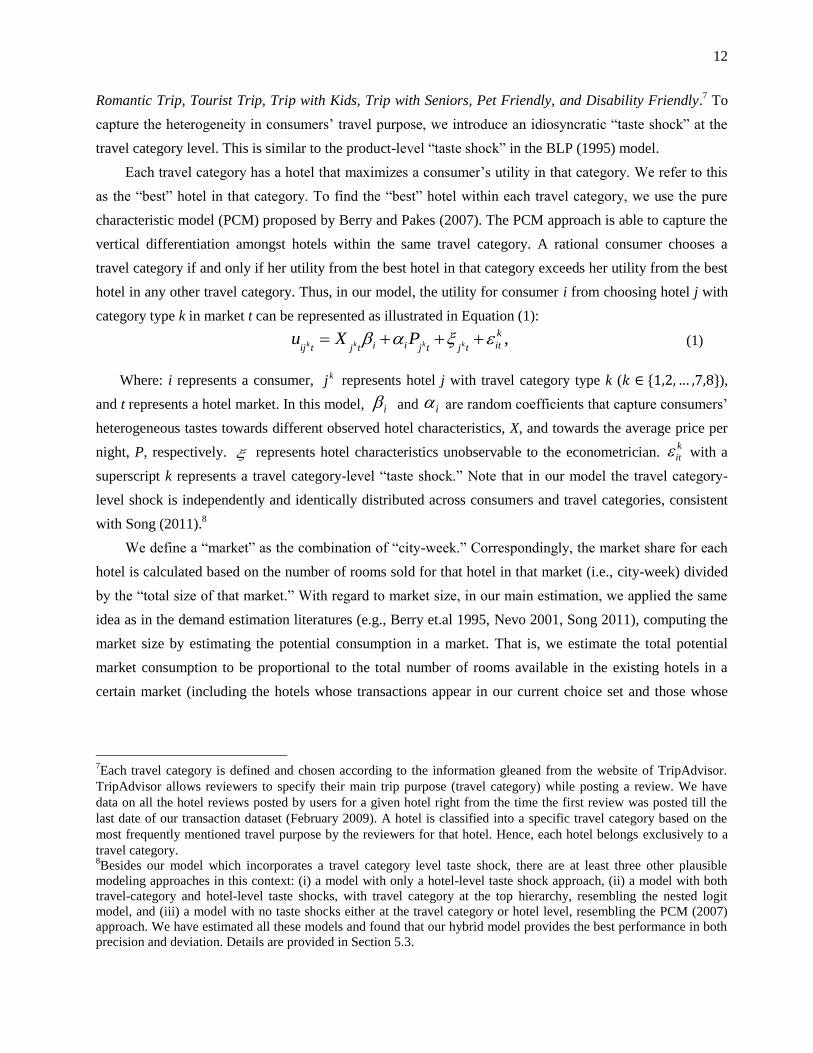
hotel in any other travel category. Thus, in our model, the utility for consumer i from choosing hotel j with

category type k in market t can be represented as illustrated in Equation (1):

,k k k k

k

i i itij t j t j t j tu X P (1)

Where: i represents a consumer, represents hotel j with travel category type k ( ),

and t represents a hotel market. In this model, and are random coefficients that capture consumers’

heterogeneous tastes towards different observed hotel characteristics, X, and towards the average price per

night, P, respectively. represents hotel characteristics unobservable to the econometrician. with a

superscript k represents a travel category-level “taste shock.” Note that in our model the travel category-

level shock is independently and identically distributed across consumers and travel categories, consistent

with Song (2011).8

We define a “market” as the combination of “city-week.” Correspondingly, the market share for each

hotel is calculated based on the number of rooms sold for that hotel in that market (i.e., city-week) divided

by the “total size of that market.” With regard to market size, in our main estimation, we applied the same

idea as in the demand estimation literatures (e.g., Berry et.al 1995, Nevo 2001, Song 2011), computing the

market size by estimating the potential consumption in a market. That is, we estimate the total potential

market consumption to be proportional to the total number of rooms available in the existing hotels in a

certain market (including the hotels whose transactions appear in our current choice set and those whose

7Each travel category is defined and chosen according to the information gleaned from the website of TripAdvisor.

TripAdvisor allows reviewers to specify their main trip purpose (travel category) while posting a review. We have

data on all the hotel reviews posted by users for a given hotel right from the time the first review was posted till the

last date of our transaction dataset (February 2009). A hotel is classified into a specific travel category based on the

most frequently mentioned travel purpose by the reviewers for that hotel. Hence, each hotel belongs exclusively to a

travel category. 8Besides our model which incorporates a travel category level taste shock, there are at least three other plausible

modeling approaches in this context: (i) a model with only a hotel-level taste shock approach, (ii) a model with both

travel-category and hotel-level taste shocks, with travel category at the top hierarchy, resembling the nested logit

model, and (iii) a model with no taste shocks either at the travel category or hotel level, resembling the PCM (2007)

approach. We have estimated all these models and found that our hybrid model provides the best performance in both

precision and deviation. Details are provided in Section 5.3.

kj

i i

k

it

13

transactions are not observed.9 Under this measure, the outside good is defined as “no purchase from the

current choice set.”

Alternatively, in our robustness checks, the market size is defined as the total number of rooms

sold from all hotels in that city during that week, based on the transaction data from Travelocity. Recall that

our main dataset comes from two sources: Travelocity-generated transaction data and TripAdvisor hotel

listing data. The dataset we used in our analysis is the set of hotels at the intersection of the two sources.

This means that the hotel choice set for each market includes those hotels that not only have a transaction

generated via Travelocity, but also have available information on user-generated reviews on TripAdvisor.

Since not every hotel that has a Travelocity-generated transaction is listed on the TripAdvisor website, we

define our “outside good” as the set of hotels that are listed in the original Travelocity transaction data, but

not listed on the TripAdvisor website.

For additional robustness checks, we tried the combination of “city-night,” “city-month” and

“state-week.” We also tried “revenue” instead of “room units” as the basis for market share calculation.

Furthermore, we also tested other ways of varying the market size. For example, we applied similar ideas

as in Song (2007), by increasing or decreasing the total size for each market by 20%. We found that all

these different measures of market size yield qualitatively the same results.

Due to the computational complexity and data restriction, estimating a unique set of weights for each

consumer is intractable. To make this model tractable, we made some further assumptions about and

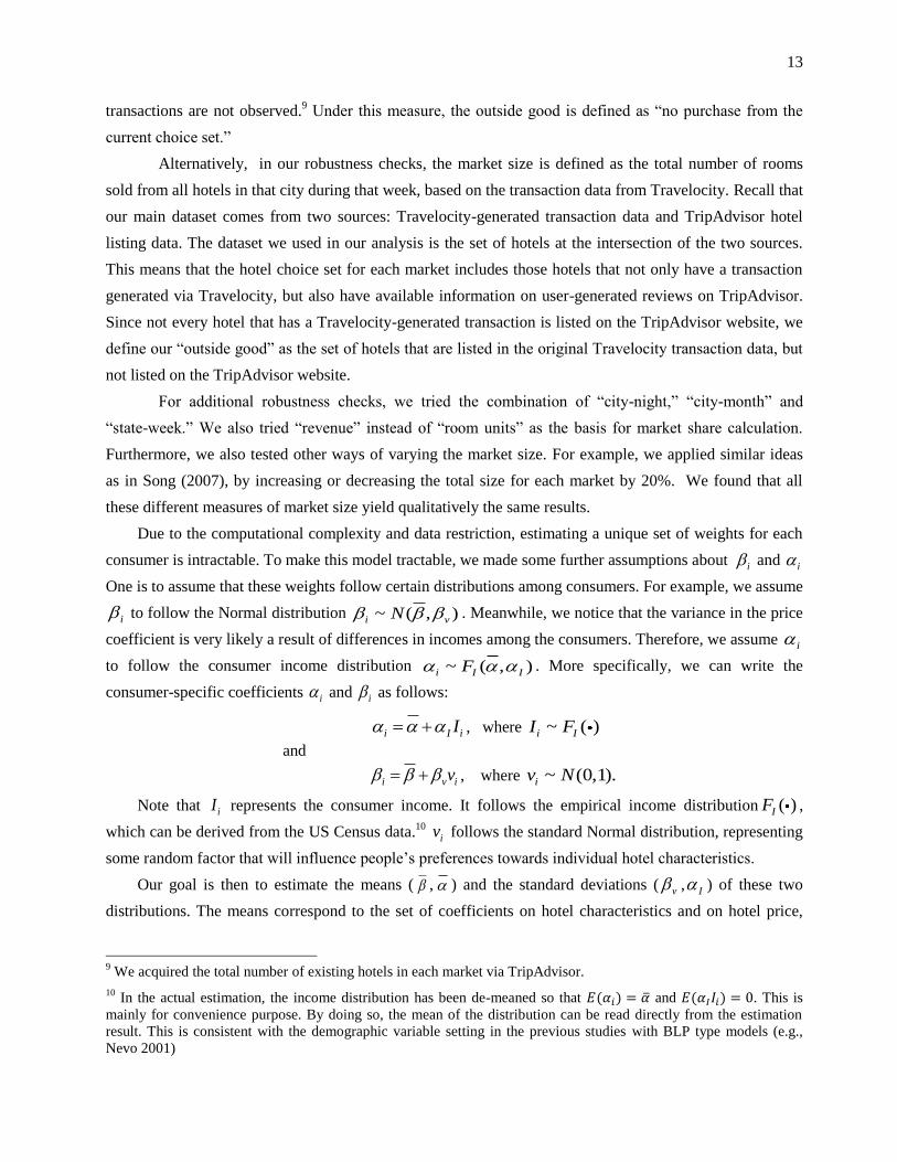
One is to assume that these weights follow certain distributions among consumers. For example, we assume

i to follow the Normal distribution ~ ( , )i vN . Meanwhile, we notice that the variance in the price

coefficient is very likely a result of differences in incomes among the consumers. Therefore, we assume i

to follow the consumer income distribution ~ ( , )i I IF . More specifically, we can write the

consumer-specific coefficients i and i as follows:

i I iI , where ~ ( )i II F

and

i v iv , where ~ (0,1).iv N

Note that iI represents the consumer income. It follows the empirical income distribution ( )IF ,

which can be derived from the US Census data.10

iv follows the standard Normal distribution, representing

some random factor that will influence people’s preferences towards individual hotel characteristics.

Our goal is then to estimate the means ( , ) and the standard deviations ( v , I ) of these two

distributions. The means correspond to the set of coefficients on hotel characteristics and on hotel price,

9 We acquired the total number of existing hotels in each market via TripAdvisor.

10 In the actual estimation, the income distribution has been de-meaned so that and . This is

mainly for convenience purpose. By doing so, the mean of the distribution can be read directly from the estimation

result. This is consistent with the demographic variable setting in the previous studies with BLP type models (e.g.,

Nevo 2001)

i i

14

which measures the average weight placed by the consumers. The standard deviations provide a measure of

the extent of consumer heterogeneity in those weights.

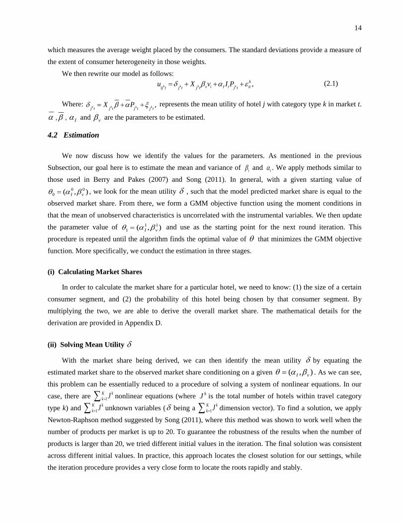
We then rewrite our model as follows:

,k k k k

k

v i I i itij t j t j t j tu X v I P (2.1)

Where: ,k k k kj t j t j t j tX P represents the mean utility of hotel j with category type k in market t.

, , I and v are the parameters to be estimated.

4.2 Estimation

We now discuss how we identify the values for the parameters. As mentioned in the previous

Subsection, our goal here is to estimate the mean and variance of and . We apply methods similar to

those used in Berry and Pakes (2007) and Song (2011). In general, with a given starting value of

, we look for the mean utility , such that the model predicted market share is equal to the

observed market share. From there, we form a GMM objective function using the moment conditions in

that the mean of unobserved characteristics is uncorrelated with the instrumental variables. We then update

the parameter value of and use as the starting point for the next round iteration. This

procedure is repeated until the algorithm finds the optimal value of that minimizes the GMM objective

function. More specifically, we conduct the estimation in three stages.

(i) Calculating Market Shares

In order to calculate the market share for a particular hotel, we need to know: (1) the size of a certain

consumer segment, and (2) the probability of this hotel being chosen by that consumer segment. By

multiplying the two, we are able to derive the overall market share. The mathematical details for the

derivation are provided in Appendix D.

(ii) Solving Mean Utility

With the market share being derived, we can then identify the mean utility by equating the

estimated market share to the observed market share conditioning on a given . As we can see,

this problem can be essentially reduced to a procedure of solving a system of nonlinear equations. In our

case, there are 1

K k

k J nonlinear equations (where is the total number of hotels within travel category

type k) and 1

K k

k J unknown variables ( being a 1

K k

k J dimension vector). To find a solution, we apply

Newton-Raphson method suggested by Song (2011), where this method was shown to work well when the

number of products per market is up to 20. To guarantee the robustness of the results when the number of

products is larger than 20, we tried different initial values in the iteration. The final solution was consistent

across different initial values. In practice, this approach locates the closest solution for our settings, while

the iteration procedure provides a very close form to locate the roots rapidly and stably.

i i

0 0

0 ( , )I v

1 1

1 ( , )I v

( , )I v

kJ

15

(iii) Solving I and v

To account for the endogeneity of price, we use a GMM estimator and form an objective function by

interacting the unobservable parameter, , with a set of instrumental variables. We use Nelder-Mead

Simplex algorithm to update the parameter values for I and v , and use as the starting points to

recalculate the market share in Step (1) and solve for the new mean utility in Step (2). This allows us to

extract the new structural error and form the GMM objective function. This entire procedure iterates until

the algorithm finds the optimal combination of I , v and that minimizes the GMM objective function.

In our case, we use average price of the “same-star rating” hotels in the other markets as an instrument

for price, similar to the approach of Hausman et al. (1994). We have tried three other sets of instruments.

First we follow Villas-Boas and Winer (1999) and use lagged prices as instruments in conjunction with

Google Trends data. The lagged price may not be an ideal instrument since it is possible to have common

demand shocks that are correlated over time. Nevertheless, common demand shocks that are correlated

through time are essentially trends. Our control for trends using search volume data for different major

hotel brands thus should alleviate most, if not all, such concerns. Second, we have also tried region

dummies as proxies for the cost (e.g., the cost of transportation, labor, etc.) as suggested by Nevo (2001).

Third, we have used BLP-style instruments. Specifically, we have used the average characteristics of the

same-star rating hotel in the other markets. All these alternate estimations yielded very similar results. The

corresponding estimation results using alternative instruments are provided in Table 3 columns 5-7. We did

an F-test in the first stage for each of the instruments. In each case, the F-test value was well over 10,

suggesting that our instruments are valid (i.e., the instruments are not weak). In addition, the Hansen’s J-

Test could not reject the null hypothesis of valid over-identifying restrictions. The detailed estimation

algorithm and the discussion for model identification are provided in Appendix E1 and E2. 11

4.3 Model Extension (1): Additional Text Features

So far we have not fully exploited the information about hotel service characteristics from the data,

which is embedded in the natural language text of the consumer reviews. For example, the “helpfulness of

the hotel staff” is a service feature that can be assessed by reading the actual consumer opinions.

Towards extracting such information, we build on the work of Hu and Liu (2004), Popescu and

Etzioni (2005), Archak et al. (2011). More details on how we extracted the text features together with the

corresponding sentimental analysis are provided in Appendix G, G-3.

11

Dube, Fox and Su (2009) note that a theoretical advantage of Newton-type methods, is that they are quadratically

convergent when the iterates are close to a local solution (e.g., Kelly 2003 and Nocedal and Wright 2006). To make

sure our estimates are reliable, we employed 50 starting points in each run of the estimation. We routinely found that

our algorithm were able to identify the same local minimum each time. Moreover, as suggested by Knittel and

Metaxoglou (2008), we also tried several alternative optimization algorithms, including (i) direct-search algorithms:

e.g., the Nelder-Mead simplex method; (ii) derivative-based algorithms: e.g., the Fletcher-Reeves conjugate gradient

method and the vector Broyden-Fletcher-Goldfarb-Shanno (BFGS) method (which is a quasi-Newton method). We

found that different algorithms were able to recover consistent structural parameters in our data.

16

4.4 Model Extension (2): Interactions with Travel Category

As discussed previously, by modeling i and i (i.e., consumer-specific coefficients towards price

and towards hotel characteristics) to be a function of consumer income ( i I iI ) and a function of

the unobserved consumer characteristic ( i v iv ), respectively, our basic model is able to take into

account the consumer heterogeneity originated from different income levels as well as from the unobserved

consumer attributes. Furthermore, to capture richer effects from consumers’ heterogeneous tastes,

demographics could potentially be added to the model in a more complex manner. This can be achieved in

a similar fashion as in Nevo (2001), by enabling interactions between travel categories and product

characteristics.

More specifically, we extend our basic model by assuming that i and i are functions of additional

consumer-level travel characteristics. In our case, we focus on consumer travel purpose. Thus, we have the

following two extended forms for the consumer-specific coefficients i and i :

i I i T iI T and ,i v i T iv T

where iT is an indicator vector with identity components representing consumer travel purpose: 12

' .i i i i i i i i iT Family Business Romance Tourist Kids Seniors Pets Disability

For example, if consumer i is on a business trip, then the corresponding travel purpose vector is

' [0 1 0 0 0 0 0 0].iT

Based on this additional assumption, the overall extended model can be thereby rewritten as

.k k k k k k

k

v i T i I i T i itij t j t j t j t j t j tu X v X T I P T P (2.2)

In the next section, we will discuss our empirical results from our basic and extended models.

5. Empirical Analysis and Results

Note that a consumer who is searching for hotel reviews on Travelocity or TripAdvisor gets to see a

different number of reviews on the pages of each website. While Travelocity.com displays the first five

reviews on a page, Tripadvisor.com lists 10 reviews per page. To minimize the potential bias caused by

webpage design, since some customers may only read the reviews on the first page, we decided to consider

two more alternatives besides our main dataset: Dataset (II) with hotels that have at least five reviews, and

12

The empirical distribution of iT can be acquired from online consumer reviews and reviewers’ profiles. Our

robustness test showed that consumers’ demographics derived from different online resources stay consistent (Jensen-

Shannon Divergence = 0.03).

17

Dataset (III) with hotels that have at least 10 reviews. Controlling for brand effect, the estimation results

from these three datasets are illustrated in Table 3 columns 2-4. As described previously, we tried several

different instruments by using lagged prices with Google Trends, various proxies for marginal costs as well

as BLP-style instruments. The corresponding results are in Table 3 columns 5-8.13

In Subsection 5.2, we discuss our robustness tests: (1) using the same model based on different

samples using alternative levels of online review data, and (2) using a different model based on the same

datasets. Then, in Subsection 5.3, we further discuss the results on model validation by comparing our

model with the current competitive ones. In Subsection 5.4, we will provide some managerial implications

by conducting counterfactual policy experiments. Finally, in Subsection 5.5, we will briefly discuss the

results from our extended model.

5.1 Results from the Basic Model

Location-based characteristics: There are five location-based characteristics, which have a positive

impact on hotel demand: “external amenities,” “beach”, “public transportation,” “highway,” and

“downtown.” These characteristics strongly imply that the location and geographical convenience for a

hotel can make a big difference in attracting consumers. Hotels providing easy access to public

transportation (such as a subway or bus stations), highway exits, restaurants and shops, or easy access to a

downtown area, can have a much higher demand. “Beach,” also showed a positive impact on demand. It

turns out that most beach-based hotels in our dataset were located in the south where the weather typically

stays warm even in winter. Therefore, the desirability of a “walkable” beachfront did not reduce even in the

winter season (which is the time of our data).

Two location-based characteristics have a negative impact on hotel demand: “annual crime rate” and

“lake/river.” The higher the average crime rate reported in a local area, the lower the desirability of

consumers for staying in a hotel located in that area. This indicates that neighborhood safety plays an

important role in the hotel industry. The second location-based characteristic that illustrates a negative

impact is the presence of a water body like a lake or a river. This is interesting because one would expect

people to choose a hotel near a lake or by a riverside. However, most waterfront-based hotels in our dataset

were located in places where the weather becomes extremely cold in the winter months of November to

January. Due to the low temperatures, it is likely that a lake or riverfront becomes less desirable for

travelers.14

13

For normalization purpose, we used the logarithms of “price,” “characteristics,” “syllables,” “spelling errors,”

“crime rate,” “internal amenities,” “external amenities” and “review count (both TripAdvisor and Travelocity)” in all

the analyses in this paper.

14In addition, some traveler reviews commented on the presence of mosquitoes in areas near a lake.

18

To further examine the impact of lake, we collected weather data from the National Oceanic and

Atmospheric Administration (NOAA) on the average temperature from 2008/11 to 2009/1 for all cities.

Then, we defined two dummy variables: “High Temp” which equals to 1 if the average temperature is

higher than 50 degree, and “Low Temp” which equals to 1 if the average temperature is lower than 40

degree.15

We interacted “High Temp” and “Low Temp” separately with “Lake” in our model. The results

showed that the interaction of “Low Temp” with “Lake” has a significantly negative effect. This supports

our earlier argument. Meanwhile, the interaction of “High Temp” with “Lake” showed a significantly

positive effect, suggesting that warmer weather may help the lake area to attract more visitors. As a

robustness check, we did the similar analysis for “Beach” conditional on high and low temperatures. The

results showed similar trend. The corresponding estimation results considering the interactions with the

temperature are shown in column 9 in Table 3.

Service-based characteristics: Both “class” and “amenity count” has a positive impact on hotel

demand. Hotels with a higher number of amenities and higher star-levels have higher demand, controlling

for price. “Reviewer rating” also has a positive association with hotel demand. With regard to the “number

of reviews,” we find a positive sign for its linear form while a negative sign for its quadratic form. This

indicates that the economic impact from the customer reviews is increasing in the volume of reviews but at

a decreasing rate, as one would expect.

Textual quality of reviews: The textual quality and style of reviews demonstrated a statistically

significant association with demand. All the readability and subjectivity characteristics had a statistically

significant association with hotel demand. Among all the readability sub-features, “complexity,”

“syllables” and “spelling errors” had a negative sign and, therefore, have a negative association with hotel

room demand. This implies that reviews with higher readability characteristics (short sentences and less

complex words), and reviews with fewer spelling errors have a positive association with demand. On the

other hand, the sign of the coefficients on “characters” and “SMOG index” is positive, implying that longer

reviews that are easier to read have a positive association with demand.16

These results indicate that

consumers can form an image about the quality of a hotel by judging the quality of the (user-generated)

reviews.

Both “mean subjectivity” and “subjectivity standard deviation” turned out to have a negative association

with demand. This implies that consumers prefer reviews that contain objective information (such as

factual descriptions of rooms) relative to subjective information. With respect to the “subjectivity standard

deviation,” our findings suggest that people prefer a “consistent objective style” from online customer

reviews compared to a mix of objective and subjective sentences. The last review-based characteristic was

15

We tried other combinations to classify High vs. Low temperatures (>=70 degrees as High and <=30 degree as Low

(ii) >=60 degrees as High and <=20 degrees as Low) but they all yielded qualitatively similar results.

16To alleviate any possible concerns with multi-collinearity between SMOG and Syllables, we re-estimate our model

after excluding the SMOG index variable. There was no change in the qualitative nature of the results across the

different datasets.

19

“disclosure of reviewer identity.” This variable demonstrated a positive association with hotel demand.

This result is consistent with previous work (Forman et al. 2008), which suggested that the identity

information about reviewers in the online travel community can shape positively community members'

judgment towards hotels. “Price” has a negative sign, which is as expected. 17

Quantitative Effects of location-, service- and review-based hotel characteristics: Besides the

above qualitative implications, we also quantitatively assess the economic value of different hotel

characteristics. More specifically, we examined the magnitude of marginal effects on hotel demand for the

location-, service- and review-based hotel characteristics. The presence of a beach near the hotel increases

demand by 17.88% on an average. In contrast, a location near a lake or river decreases demand by 13.18%.

Meanwhile, easy access to transportations and highway exits increase demand by 18.44% and 7.99%,

separately. Presence of a hotel near downtown increases demand by 4.94%. With regard to service-based

characteristics, a 1-star improvement in hotel class leads to an increase in demand by 3.89% on average.

Moreover, the presence of one more internal or external amenity increases demand by 0.06% or 0.08%,

respectively. Demand decreases by 0.27% if the local crime rate increases by one unit.

With regard to the review-based characteristics, we found that the SMOG index (which represents the

readability of the review text), has the highest marginal influence on demand on an average. A one level

increase in SMOG index of reviews is associated with an increase in hotel demand by 8.83% on an

average. A one unit increase in the number of characters is associated with an increase in hotel demand by

0.11%, whereas a one unit increase in the number of spelling errors, syllables or in complexity is associated

with a decrease in hotel demand by 1.44%, 0.45%, and 1.18%, respectively. In terms of review subjectivity,

a 10 percent increase in the average subjectivity level is associated with a decrease in hotel demand by

1.66%; a 10 percent increase in the standard deviation of subjectivity will reduce demand by 4.88%.

Finally, a 10 percent increase in the reviewer identity-disclosure levels is associated with an increase in

hotel demand by 0.63%.

Note that the estimation results from the three datasets are highly consistent. In general, all the

coefficients illustrate a statistical significance with a p-value equal to or below the 5% level across all three

datasets. Moreover, a large majority of variables present a high significance with a p-value below the 0.1%

level.

5.2 Robustness Checks

To assess the robustness of our estimation model and results, we report two additional groups of tests.

(i) Robustness Test I: Use the same model based on alternative sample splits.

17

In addition, we also considered “Airport,” “Convention centers” and “Number of rooms”. The estimation results are

consistent with our current results, but the coefficients for the two characteristics are statistically insignificant.

20

We considered three alternative datasets: Dataset (IV) containing hotels with at least one review from

TripAdvisor.com, Dataset (V) containing hotels with at least one review from Travelocity.com, and Dataset

(VI) containing hotels with at least one review from both. The results are in Appendix A, Table A1. We

found that the coefficients from the estimations are qualitatively very similar to our main results. Moreover,

similar to those in the main results, most variables in the robustness tests also illustrate statistical

significance at or below the 5% level or stronger. Thus, our estimation results, based on the hybrid random

coefficient model, are quite consistent across different datasets.

(ii) Robustness Test II: Use an alternative model based on the same datasets.

To examine the robustness of the results from our model, we conducted another group of tests using

an alternative model that has been widely used in the industrial organization and marketing literature, the

random coefficient logit model, or BLP (Berry et al. 1995). As mentioned in Section 4, the key difference

between the BLP approach and our model is that BLP introduces a demand “taste shock” at each product

level (in our case, hotel), rather than at a group level (in our case, the travel category), as in our model.

Consequently, the substitution space for BLP is different in the sense that BLP does not distinguish

between the two types of cross substitutions - the “within-travel category” and “between-travel category.”

Rather, it would treat all hotels as possible substitutes. We added two sets of dummy variables, one for

brand and the other for travel category. We conducted the same set of estimations based on Datasets (I) -

(VI).

The results are in columns 2-7 in Table A2 in Appendix A. In addition to an alternate specification

with homogeneous coefficients on the travel category dummies, we further considered consumers’

heterogeneous preferences by assigning random coefficients to these dummies. The corresponding results

are shown in the last column in Table A2 in Appendix A.

We find that the estimation results from the BLP model are consistent with our main estimation results

using the hybrid model. Specifically, the coefficients from the BLP estimation demonstrate three trends: (i)

they have the same signs compared to our main results from the hybrid model, which means that the

economic effects are consistent in direction, (ii) they exhibit lower levels of statistical significance,

compared to our main results, and (iii) the magnitude of these coefficients is generally higher compared to

our main results. These three trends are also very consistent with the findings in Song (2011). In the next

Subsection, our model validation results further confirm this finding.

(iii) Robustness Test III: Causal effect of UGC

To alleviate concerns regarding whether UGC has a causal effect on demand or not, we conducted an

additional robustness test using a regression discontinuity (RD) design as suggested by Luca (2010). More

specifically, our test builds on the special “rounding mechanism” used by both Travelocity and

TripAdvisor. These two websites generate their overall rating for each hotel by rounding the average

21

review ratings to the closest half star. For example, if the average rating across all reviewers is 3.24, then it

will be rounded to 3; if the average rating is 3.25, then it will be rounded to 3.5. Thus, we looked at those

hotels with an unrounded average rating just below and just above each rounding threshold. Then we

looked for whether or not there exists a discontinuous jump in the sales pattern that follows the

discontinuous jump in the website-displayed rounded overall rating, while controlling for the continuous

unrounded rating and other hotel characteristics. Similar to Luca (2010), this design is based on the

assumption that all sale-affecting predetermined characteristics of hotels become increasing similar, when

getting closer to both sides of a rounding threshold. We found a significant positive treatment effect

suggesting that keeping everything else the same, the discontinuous pattern found in the sales is caused by

the discontinuous pattern in the rating. This strongly suggests that user-generated reviews have a causal

impact on hotel demand.

As a robustness check, we tried different bandwidths (bin size) of the neighborhood near the rounding

threshold. We found that our results are quite consistent and not sensitive to the bin size. Moreover, to

eliminate the possibility of self-selection bias (e.g., as addressed by Hartmann, Nair & Narayanan (2010))

that could potentially invalidate the RD design (For instance, hotels may submit the reviews themselves to

pass the threshold), we performed an additional McCrary density test (McCrary 2008) as suggested by

Luca (2010). In particular, we divided the overall range of rating into small bins with a range of 0.05. Then

we checked if the density for the number of submitted reviews is disproportionately large in the bins which

are just above the rounding threshold (e.g., 3.25-3.3). This is because if hotels are gaming the system and

submitting reviews themselves, one would expect to see a disproportionately large amount of reviews just

above the rounding threshold. We did not find any significant difference in the density from our data,

suggesting no evidence for hotel “gaming” behavior.

In summary, the additional robustness tests using RD design together with McCrary density test allow

us to derive higher confidence in the causal impact of online reviews on product demand. Given these tests,

it is unlikely that the causal effect is in the other direction (e.g., certain types of hotels will generate certain

types of online reviews, no matter whether it is in terms of the ratings, the style of reviews, or the textual

content of the reviews).

5.3 Model Comparison

For model comparison purposes, we estimated three baseline models: the BLP model, the PCM model

and the nested logit model with travel category at the top hierarchy. Based on the previous study by Steckel

and Vanhonacker (1993), we randomly partitioned our main sample Dataset (I) into two parts: a subset with

70% of the total observations as the “estimation sample,” and a subset with 30% of the total observations as

the “holdout sample.” To minimize any potential bias from the partition procedure, we performed a 10-fold

cross-validation. We conducted this validation process for our random coefficient model and the three

22

baseline models. Furthermore, to examine the model’s ability to capture a deeper level of consumer

heterogeneity, we compared an extended version of our model with an extended version of the BLP model

when incorporating additional interaction effects (i.e., travel purpose interacted with price and hotel

characteristics). Besides, to examine the significance of the UGC-based, the location-based and the

service-based hotel characteristics, we compared with the original model fit by using the same hybrid

model but excluding the UGC, location, and service variables, separately. Finally, to evaluate the

usefulness of different aspects of UGC in modeling the demand, we further conducted model comparison

using hybrid model but excluding the numerical ratings and the textual review features, respectively. We

also evaluated models without each of the textual features, such as readability, subjectivity and reviewer

identity variables, separately. We have done the above work for both in-sample and out-of-sample

comparisons. The results are provided in Table B1 to B8 in Appendix B. 18

The results showed that a model that conditions on UGC variables significantly improves the model

predictive power. With respect to out-of-sample RMSE, the model fit improves by 35.80% when add the

UGC variables. Similar trends in improvement in our model fit occur with respect to the other two metrics,

MSE and MAD in both in-sample and out-of-sample analyses.

Our out-of-sample results in Table B5 illustrate that our model improves by 10.51% in RMSE

compared to the BLP model with no random coefficients on travel category dummies. This number

becomes 53.04%, 61.65%, and 8.46% with respect to the PCM, the Nested Logit model, and the BLP

model with random coefficients on travel category dummies, respectively. Thus, our model provides the

best overall performance in both precision (i.e., RMSE, MSE) and deviation (i.e., MAD) of the predicted

market share. The nested logit model presents the worst performance in the predictive power. Moreover, as

illustrated in Table B6, when incorporating interaction effects, although both models show improvement in

predictive power, the extended hybrid model performs much better than the extended BLP model.

From Table B7 we find that by including the UGC, location-based, and service-based variables, our

model fit improves by 35.80%, 55.06%, and 52.43% in RMSE. Similar trends in improvement in our model

fit occur with respect to the other metrics, MSE and MAD. Therefore, our results suggest that the model

predictive power will drop the most if we were to exclude the location-based variables from our model,

followed by the service-based variables, and finally followed by the UGC variables. This strongly indicates

that location- and service-based characteristics are indeed the two most influential factors for the hotel

demand.

18

With regard to the unobserved characteristics required for out-of-sample prediction using the hybrid, BLP and PCM

models, we applied the same method as suggested in Athey and Imbens (2007). We drew the unobserved

characteristics for the “holdout sample” randomly from the marginal distribution of unobserved characteristics

estimated from the “estimation sample”. This method has also been used in the Marketing literature. See for example,

Nair, Dube and Chintagunta (2005) who infer the structural error for the "hold out" sample from the marginal

distribution of the structural error across different markets derived from the "estimation" sample.

23

Moreover, from Table B8, we find that amongst all the UGC-related features, textual information

has significantly higher impact on the model predictive power than the numerical features. The former

improves the model fit by 33.77% in RMSE, compared to an increase of 17.93% by the latter. In addition,

within the set of textual features, we find the readability and subjectivity of reviews show a higher impact

compared to the reviewer identity information.

5.4 Counterfactual Experiments

A key advantage of structural modeling is its potential for normative policy evaluation. To measure

explicitly the economic impact of strategic policies, we conducted various counterfactual experiments.

Specifically, we simulated the following two sets of scenarios.

(i) Counterfactual Experiment I: Effects of price cut under different location environments.

To examine how pricing policy change will affect hotel demand under different location

environments, we conducted the second set of counterfactual experiments. First, we generated 6 derivative

samples, by assuming each of the following 6 location features to be absent, beach, downtown, highway,

lake, transportation, and external amenities, one at a time. Then, we assumed a price cut by 20% for each

environment and examine the demand change. Our finding showed that the increase of hotel demand is the

lowest in areas with no highway compared to others. This low price elasticity suggests that in such areas

consumers tend to be less sensitive to price cut.

Furthermore, we consider two additional types of location feature combinations: (1) Beach and

highway (which represents the typical west/south coast setting), and (2) Downtown, transportation and

external amenities (which represents the typical big city setting). Correspondingly, we generated two

derivative datasets by assuming all other location features that are not in the combination to be absent for

each case. Again, we re-computed the utilities and re-estimated the model. Results show that the increase in

demand is 21% lower in big city setting than that in coastline setting. Consumers tend to react much less

sensitively to hotel price in big cities. This strongly indicates that price change in big cities may not be an

effective strategy in adjusting hotel demand, compared to that in coastline areas.

(ii) Counterfactual Experiment II: Effects of price cut on substitution pattern.

In the third set of experiments, we looked into how price change in one type of hotels will affect the

demand for other types of hotels. Specifically, we focused on hotels with different star ratings.

We assumed a price cut by 20% for all 4-star hotels. By doing so, we tried to find out what are the

demand changes for the 5-, 3-, 2-, 1-star hotels. Our results showed that under the experimental setting, the

demand for 4-star hotels will increase 2.90%, while the demand for hotels from all other classes will

decrease. Among all of them, the demand for 5-star hotels drops the most with a rate of 5.34%, followed by

3-star hotels with a rate of 3.88%. The negative impacts on the demand for 1-star and 2-star hotels are

24

relatively smaller, with a rate of 2.87% and 2.60%, respectively. Meanwhile, we also conducted similar

analyses for hotels from other classes. For example, by assuming a 20% price cut for the 3-star hotels, we

found that the demand for 3-star hotels will increase by 2.79%. As a result, the demand for 4-star and 2-star

hotels will drop the most, with a rate of 5.14% and 5.01%, respectively.

From the above set of experiments, that the basic findings are as follows: (i) a price cut for a particular

class of hotels tends to cause a demand drop for all the hotels in the lower-level class(es) and (ii) the closest

substitutes for 4-star hotels are 5-star hotels; the closest substitutes for 3-star hotels are 4-star and 2-star

hotels; the closest substitutes for 2-star hotels are 1-star hotels.

5.5 Estimation Results from Model Extensions

As discussed in sections 4.3 and 4.4, we also empirically estimated the two extended models.

(i) With additional text features

The estimation results for the extended model with additional text features are shown in Table 4. We

see that the qualitative nature of our main results remains the same. In addition, we see that the three

features that have a positive and statistically significant impact on demand are “food quality,” “hotel staff”

and “parking facilities.” In contrast, “bedroom quality” had a negative impact on demand. While this

negative sign is surprising, this can happen if consumers use bedroom quality as a cue for price, especially

given that quality in our data is a proxy for the number of beds and size of the room (full, queen, king, etc).

This is possible because sometimes prices are obfuscated on the main results page and are only available

just before checkout. However, this is only one possible explanation.

(ii) With interaction effects

The additional interaction effects enable us to understand better how the distribution of consumers’

heterogeneous preferences is influenced by the distribution of consumers’ demographic information. More

specifically, we focused on estimating three sets of interaction effects:

1) Interaction between Travel Category and Price;

2) Interaction between Travel Category and Hotel Characteristics (e.g., location, service, brand, etc.);

3) Interaction between Unobserved Consumer Characteristics and Hotel Characteristics.

The corresponding results for these three sets of interaction effects are provided in Table 5b, Table 5c,

Table 5d and Table 5e. 19

The estimated mean coefficients are shown in Table 5a.

First, we notice that consumers’ heterogeneous tastes towards price can be explained by their travel

purposes. For example, from Table 5a, we know that the mean price coefficient is -0.121. Thus, from Table

19

We also estimated the interaction effects between Income and Price. The corresponding results are available from

the authors upon request.

25

5b, we can infer that if a consumer is on a business trip, her price coefficient will increase by 0.027 above

the mean, which yields an adjusted price coefficient of -0.094. In contrast, if a consumer is on a family trip

or a romance trip, her adjusted price coefficient is -0.133 or -0.126, respectively. Among all different types

of travelers, we found that tourists (i.e., travelers on a large group tour) tend to be the most price-sensitive

with an adjusted price coefficient of -0.139, whereas business travelers are the least price-sensitive. These

findings are consistent with those from the marginal effects of price change on demand. For instance, we

find that a 20% increase in hotel price will lead to a 1.58% demand drop from business travelers, compared

to a 2.22% drop from family travelers, a 2.11% demand drop from romance travelers, and a 2.32% demand

drop from tourists.

Furthermore, we find that consumer heterogeneity towards different hotel location and service

characteristics is also influenced by travel purpose. For instance, we notice that business travelers have the

highest marginal valuation for “highway” and “public transportation.” In other words, hotels with easy

access to interstate highway or public transportations are most attractive to business travelers. From Table

5a, we see that the mean coefficients for “highway” and “transportation” are 0.066 and 0.158, respectively.

According to the estimated interaction effects in Table 5c, we can infer that for business travelers the

presence of “highway” and “transportation” weigh significantly higher than the mean coefficients, with an

increase of 0.101 and 0.134 for each. Correspondingly, the presence of interstate highway near a hotel will

increase hotel demand from business travelers by 17.43%, compared to a 6.89% demand increase for the

average traveler, and a 4.07% demand increase from romance travelers. Similarly, the presence of public

transportation near a hotel will increase hotel demand from business travelers by 33.03%, compared to a

17.87% demand increase for the average traveler, and a 9.05% demand increase from family travelers.

In contrast, romance travelers are more sensitive to “hotel class” and “beach” compared to other types

of travelers. For example, the presence of beach near a hotel will increase hotel demand from romance

travelers by 27.69%, compared to a 17.81% demand increase for the average traveler, and a 12.97%

demand increase from business travelers. Similarly, a 1-star improvement in hotel class will lead to an

increase in hotel demand from romance travelers by 19.53%, compared to a 6.06% demand increase for the

average traveler, and a 2.57% demand increase from tourists.

Finally, as shown in Table 5e, we also notice that after accounting for the interaction effects, the

estimates on the unobserved consumer characteristic (i.e., vi) become insignificant at conventional

significance levels (compared to its being statistical significance in the basic model without the interaction

effects). This finding is consistent with Nevo (2001), which suggests that most of the consumer

heterogeneity is explained by the observed demographics, rather than the unobservable.

6. Utility-Based Hotel Ranking

26

After we estimate the parameters, we can derive the utility gain that a consumer with a particular

travel purpose receives from paying for a given hotel. Thereafter, we propose to design a new ranking tool

for hotels based on the average utility gain from transactions in that hotel. As discussed in Section 4, to

capture the consumer heterogeneity, we represent the utility from each hotel for each consumer as

consisting of two parts: the mean and the deviation. The mean utility provides us with a good estimation of

how much consumers can benefit from choosing this particular hotel, while the deviation of utility

describes the variance of this benefit. In our case, we are interested in knowing what the utility gain is for

consumers on an aggregate level from choosing a certain hotel. Therefore, we define the average utility

gain from hotel j with travel category type k as the sum of its mean utility, defined in Eq. (2.1) over all

markets:

kk j tj

t

Utility Gain (3)

6.1 Ranking Hotels

We thereby propose a new ranking approach for hotels based on the utility gain from each hotel for

consumers on an aggregate level. If a hotel provides a comparably higher average utility gain, then it would

appear on the top of our ranking list. Using the coefficients for hotel characteristics estimated from our

model, we are able to compute the average utility gain based on Eq. (3). Notice that in this equation, kj t is

the average value of the estimated utility gain over the consumer population in market t:

1( ),

Nk

kj t k k v i I i k itj t j t j ti

X v I PN

(4)

where N represents the total number of consumers involved in the estimation, This definition takes into

account all of the sources of uncertainty including the random coefficients, the model errors, etc. Since by

assumption k

k v i I i k itj t j tX v I P is mean-zero (e.g., Nevo 2001), in our actual computation, Eq. (4)

can be simplified as

1( ).

N

kj t kj tiN

(5)

Using the estimates from the previous analysis, we are able to compute kj t . Thus, the final average

utility gain, kjUtility Gain , is then computed by summing over kj t across all markets. Used as the final

ranking criterion, the average utility gain provides us with the best valuation on the hotel cost performance

and provides customers with the best-valued hotels, consequently.

6.2 User Study Based on Lab Experiments

To evaluate the quality of our ranking technique, we conducted an extensive user study towards which

we designed and executed several lab experiments using Amazon Mechanical Turk. We computed the

27

expected utility for each hotel from our parameter estimates, and ranked the hotels in each city according to

their average utility gain. Then we generated different rankings for the top-10 hotels in accordance with

several existing baseline criteria deployed by travel search engines: Most booked, Price low to high, Price

high to low, Hotel class, Hotel size (number of rooms), and Number of internal amenities. We also

considered 4 other benchmark criteria based on user-generated content: Customer rating from

TripAdvisor.com, Customer rating from Travelocity.com, Mixed rating from TripAdvisor.com and

Travelocity.com 20

, and Maximum online review count. Moreover, to examine the significance of the UGC

and of the comprehensive model to the overall performance of the ranking scheme, we generated two more

baselines using the same hybrid model but excluding all the UGC variables, and using the BLP model (as

described in Subsection 5.2). Finally, we also generated a “Combined ranking" using combined criteria of

“price” and “hotel class” to examine whether a ranking that attempts to introduce diversity artificially can

compete with our utility-based one. We did this by interlacing the top-5 hotels with “the lowest price” and

the top-5 hotels with “the highest number of stars.”21

We presented our model generated ranking together with one of the above-mentioned alternative

rankings and asked users to compare each pair of rankings, i.e., our ranking paired with one of the existing

benchmarks. To avoid any potential bias, we did not release any information to the users about the criteria

for generating those rankings and randomized the orders of presentation of the rankings. The studies in our

ranking evaluations were blind, pair-wise, tests, in which the two rankings were presented side by side, and

the user had to pick one of them, without having any further information beyond the list of the hotels in

each. This resulted in a total of 13 different experiments for each of the six cities (Los Angeles, New

Orleans, New York, Orlando, San Francisco, and Salt Lake City) resulting in a total of 78 experiments each

having 200 participants and involved more than 15,600 user comparisons of different ranking lists.

To further control for any experimental design biases and to test the robustness of our findings, we

then conducted another set of similar experiments with more stringent controls in the design and execution

of the experiment. This led to a set of 7800 user comparisons. More details on the second experiment are

provided in Appendix C. We found that with the additional controls, the second experiment provided very

consistent results with the results from our first experiment.

Due to brevity, we only provide details from the second, tighter version of the experiment. Our results

showed that for each of the 13 comparisons in each of the 6 cities, the majority of customers preferred our

ranking, when listed in a blind setting, side-by-side with the other competing baseline techniques (p = 0.05,

20

Since some hotels have zero reviews, we considered a mixed approach for their ratings. More details are provided in

Table 6. 21

We also tried interlacing rankings with different criteria, such as “the highest price” and the “lowest number of

stars,” or “the lowest price” and the “lowest number of stars,” or “the highest price” and the “highest number of

stars.”The results are similar. This suggests that customers prefer a list of hotels that specialize in a variety of

characteristics, rather than a variety of hotels that each specialize in only one characteristic.

28

sign test). Table 6 shows our results after controlling for additional factors, indicating how often users

preferred our own ranking scheme when presented side-by-side with an alternative. Notice that in all 78

experiments, we observe a statistically significant difference for our ranking (p = 0.05, sign test). The

overall set of results (in none of the 78 experiments our ranking was deemed worse), is a strong indication

that our ranking strategy is preferable to the existing baselines. A screenshot for sample tasks from the

experiment is provided in Figure C1 Appendix C. Moreover, our ranking based on the hybrid model with

UGC variables was preferred over the one without UGC variables, and over the one generated based on the

BLP model. This further demonstrates the importance of incorporating UGC variables in any demand

estimation model that generates a ranking system.

As part of this study, we also asked consumers why they chose a particular ranking. This was done to

better understand how users interpret the utility-based ranking. The majority of users indicated that our

utility-based ranking promoted the idea that price was not the main factor in rating the quality of hotels.

Instead, a good ranking recommendation is one that could satisfy customers' multidimensional preferences

for hotels. Moreover, users strongly preferred the diversity of the retrieved results, given that the list

consisted of a mix of hotels cutting across several price and quality ranges. In contrast, the other ranking

approaches tended to list hotel of only one type (e.g., very expensive for “star ratings,” or mainly 3-star

hotels for “most booked”). Notice that even the ranking baseline with the combined criteria showed the

similar trend. This further indicates that customers prefer a list of hotels that each specializes in a variety of

characteristics, rather than a variety of hotels that each specializes in only a few characteristics.

Of course, diversity of results is well-known to be a factor of user satisfaction in web search

(Agichtein 2006). While we could potentially try to imitate solutions from web search and introduce

diversity in the results in an exogenous manner, we observe that the approach based on “consumer utility”

theory introduces diversity naturally in the results. This result seems intuitive: if a specific segment of the

market systematically appears to be underpriced, hence introducing a non-diverse set of results, then

market forces would modify the prices for the whole segment accordingly. Thus, these results dovetail well

with our empirical estimation, which suggests that our utility-based ranking model can capture consumers'

true purchase motivations.

Moreover, our user study indicates that a star-rating system would not come close to achieving the

same goal. Apparently one could interpret a subject’s star-rating as a discrete approximation of her utility

for a hotel, thus ranking based on star-rating ought to perform as well as ranking based on utility as the

latter is just a money-metric transformation of the former. However, this is not true. The reason is that the

matching of consumers to hotels in star rating systems is not random. A consumer only rates the hotel that

she has already chosen before (i.e., the one that maximizes her perceived utility gain). Consequently, the

average star rating for each hotel need not reflect the population average utility but rather the satisfaction of

consumers with their own choices. Thus, rankings based on average star ratings need not reflect a ranking

based on average utility.

29

7. Conclusions and Implications

In this paper, we estimate the economic value of different hotel characteristics, especially the location-

based and service-based characteristics, given the associated local infrastructure. We propose a random

coefficient hybrid structural model, taking into consideration the two sources of consumer heterogeneity

introduced by the different travel occasions and different hotel characteristics. Combining this econometric

model with UGC data, using techniques from text mining, image classification, social geo-tagging, human

annotations and geo-mapping tools, we examine a unique dataset consisting of actual transactions for hotels

located in the US and infer the economic impact of various hotel characteristics. We then incorporate them

into a new hotel ranking system based on the derived average utility gain. By doing so, we can provide

customers with the “best-value" hotels early on, hence, improving the quality of local searches for such

hotels. The estimation models are privacy-friendly as they do not require individual consumer data but

rather rely on aggregate data.

On a broader note, the objective of this paper was to illustrate how UGC on the Internet can be mined

and incorporated into a demand estimation model. Our inter-disciplinary approach can provide insights for

using text mining and image classification techniques in economics and marketing research.

Simultaneously, such research can also highlight the value of using an economic context to computer

scientists to estimate both the intensity and the polarity of the UGC, especially in reviews and blogs.

Towards this, we empirically estimated the economic value of different hotel characteristics, including both

service based and location-based characteristics, from multiple sources of UGC.

Our research enables us to not only quantify the economic impact of hotel characteristics, but also, by

reversing the logic of this analysis, enables us to identify the characteristics that most influence demand for

a particular hotel. After inferring the economic significance of each characteristic, we incorporate them in a

model of expected utility gain estimation. The end goal is to generate a ranking system that recommends

hotels providing the best value for money on an average. The key idea is that hotels (or products in general)

that provide consumers with a higher surplus should be ranked higher in response to consumer queries. We

conducted blind tests using real users, recruited through AMT to examine how well our ranking system

performs in comparison with existing alternatives. We find that our ranking performs significantly better

than several baseline-ranking systems that are being currently used.

We should also note that our ranking scheme is “causal,” in the sense that the model can predict what

“should” happen when we observe changes in the market. For example, when we see a new product in the

marketplace, we can rank it by simply observing its characteristics, without waiting to see the consumers’

demand for the product. Further, we can dynamically change the rankings as a reaction to changes in the

products. For example, if we observe a price change, or if we observe that a hotel closes its pool for

renovations, we can adjust immediately the surplus values and re-estimate the rankings.

30

Such research can provide us with critical insights into how humans make choice when exposed to

multiple ranked lists of choices on the same computer screen. Furthermore, by examining product search

through the “economic lens” of utilities, we leverage and integrate theories of relevance from information

retrieval and micro-economic theory. Our inter-disciplinary approach has the potential improve the quality

of results displayed by any product search engine and improve the quality of choices available to

consumers on the Internet.

In order to better understand the antecedents of consumer’s decisions, future work can look not only at

transaction data but also into their browsing history and learning behavior. For example, our current model

assumes that consumers are engaging into optimal utility maximizing behavior. However, this is not always

true, as some consumers are more thorough than others in their search. By leveraging browsing histories,

we can build models that explicitly take into consideration the fact that some users are “utility optimizers”

and some others simply engage in “satisficing” behavior. It would be also interesting to examine the

difference in the conversion rate of users, when presented with surplus-based rankings.

Our work has several limitations some of which can serve as fruitful areas for future research. One can

further break down the textual content of user-generated reviews in order to extract multiple service

amenity related dimensions of every single hotel and examine the economic impact of each amenity. This

can be done by conducting auto topic extraction techniques from text mining, combining with sentimental

analysis to evaluate the subjectivity level of each interesting topic. This will enable us to better recover

customers’ multi-dimensional heterogeneous tastes towards different product characteristics. In order to

better understand the antecedents of consumer’s decisions, future work can look not only at transaction data

but also into their browsing history and learning behavior. Furthermore, by incorporating more individual

level demographics and context information from the time of purchase, one can extend our techniques to

infer utilities at a more personalized level. This will enable one to improve the evaluation process by

comparing our recommendations with the results from the traditional collaborative filtering or content-

based algorithms. Our model also has limited structure with regard to competition, which does not allow us

to study the impact of entry-exit decisions of hotels in different regions. In our model, the travel category-

level shock is independently and identically distributed across consumers and travel categories. However,

there could also be correlations in the travel category shocks wherein a consumer combines multiple

purposes in one trip occasion.22

While our model does not capture this, it is a promising area for future

work.

22

We thank an anonymous reviewer for pointing this out.

31

References

Agichtein, E., Brill, E., Dumais, S., Ragno, R., 2006. Learning User Interaction Models for Predicting Web Search Result Preferences. Proceedings of the 29th annual international ACM SIGIR conference on Research and development in information retrieval pp 3-10.

Ansari, A., C. Mela. 2003. E-customization. Journal of Marketing Research, 40(2) 131-145.

Ansari, A., S. Essegaier, R. Kohli. 2000. Internet Recommendation Systems, Journal of Marketing Research, 37, pp. 363-375.

Archak, N., A. Ghose and P.G. Ipeirotis. 2011. Deriving The Pricing Power Of Product Features By Mining Consumer Reviews, Management Science, Forthcoming.

Arnaud, D. B., J. Liechty, E. Huizingh, G. Lilien. 2008. Offering Online Recommendations with Minimum Customer Input Through Conjoint-Based Decision Aids. Marketing Science, 27(3), pp. 443-460.

Athey, S., G. Imbens. 2007. Discrete Choice Models with Multiple Unobserved Choice Characteristics. International Economic Review, 48(4), pp. 1159-1192.

Berndt, E. 1996. The Practice of Econometrics: Classic and Contemporary, Addison-Wesley Publishing Company, Reading, MA.

Berry, S. 1994. Estimating Discrete Choice Models of Product Differentiation. RAND Journal of Economics (25). Pp. 242-262.

Berry, S., J. Levinsohn, A. Pakes. 1995. Automobile Prices in Market Equilibrium. Econometrica (63). Pp. 841-890.

Berry, S., O. Linton, A. Pakes. 2004. Limit Theorems for Estimating the Parameters of Differentiated Product Demand Systems. Review of Economic Studies (71). Pp. 613-654.

Berry, S. and A. Pakes. 2007. The Pure Characteristics Demand Model. International Economic Review (48). Pp. 1193-1225.

Bodapati, A. 2008. Recommender Systems With Purchase Data. Journal of Marketing Research, 45 (1), 77--93.

Chevalier, J., D. Mayzlin. 2006. The Effect Of Word Of Mouth On Sales: Online Book Reviews. J. Marketing Res. 43(3) 345-354.

Chintagunta 2001. Research Note Endogeneity and Heterogeneity in a Probit Demand Model: Estimation Using Aggregate Data. Marketing Science, 20(4), 442-456.

Chintagunta, P., J.P. Dubé, K.Y. Goh. 2005. Beyond the Endogeneity Bias: The Effect of Unmeasured Brand Characteristics on Household-Level Brand Choice Models. Management Science Vol. 51, No. 5, May 2005, pp. 832-84.

Chung, T.S., R. Rust, M. Wedel. 2009. My Mobile Music: An Adaptive Personalization System For Digital Audio Players, Marketing Science, 28 (1), 52--68.

Das, S., M. Chen. 2007. Yahoo! For Amazon: Sentiment Extraction From Small Talk on the Web. Management Science 53(9) 1375–1388.

Decker, R., M. Trusov. 2010. Estimating Aggregate Consumer Preferences From Online Product Reviews. International Journal of Research in Marketing 27(4) 293–307.

Dellarocas, C., N. Awad, M. Zhang. 2007. Exploring The Value of Online Product Reviews In Forecasting Sales: The Case Of Motion Pictures. J. Interactive Marketing 21(4) 23-45.

Duan, W., B. Gu, A. B. Whinston. 2008. Do Online Reviews Matter? An Empirical Investigation of Panel Data. Decision Support Systems 45(4) 1007-1016.

Dube, J.P., J. Fox, L. Su 2009. Improving the Numerical Performance of BLP Static and Dynamic

32

Discrete Choice Random Coefficients Demand Estimation, Working Paper, University of Chicago.

Eliashberg, J., S. K. Hui, Z. J. Zhang. 2007. From Story Line To Box Office: A New Approach For Green-Lighting Movie Scripts. Management Sci. 53(6) 881–893.

Fader, P. S., B. G.S. Hardie. 1996. Modeling Consumer Choice Among SKUs. Journal of Marketing Research, 33 (November), pp. 442-452.

Fellbaum, C. 1998. Wordnet: An Electronic Lexical Database. MIT Press.

Forman, C., A. Ghose, B. Wiesenfeld. 2008. Examining The Relationship Between Reviews And Sales: The Role Of Reviewer Identity Disclosure In Electronic Markets. Inform. Systems Res. 19(3) 291-313.

Franklin, S., M. Wulder. 2002. Remote Sensing Methods In Medium Spatial Resolution Satellite Data Land Cover Classification Of Large Areas, Progress in Physical Geography (26), pp. 173-205.

Fukuda, S., H. Hirosawa. 2001. Support Vector Machine Classification Of Land Cover: Application To Polarimetric SAR Data, in Proceedings of the IEEE International Geoscience & Remote Sensing Symposium, pp. 187-189.

Ghose, A. 2009. Internet Exchanges For Used Goods: An Empirical Analysis of Trade Patterns And Adverse Selection. MIS Quarterly 33(1) 1-30.

Ghose, A., P.G. Ipeirotis. 2011. Estimating The Helpfulness And Economic Impact Of Product Reviews: Mining Text And Reviewer Characteristics. Forthcoming, IEEE Transactions On Knowledge And Data Engineering.

Ghose, A., P.G. Ipeirotis, A. Sundararajan. 2006. The Dimensions of Reputation in Electronic Markets. Working Paper, New York University.

Godes, D., D. Mayzlin. 2004. Using Online Conversations To Study Word of Mouth Communication. Marketing Science. 23(4) 545-560.

Hartmann, W., Nair, H.S., and Narayanan, S. 2010. Nonparametric Identification of Causal Marketing-Mix Effects Using a Regression Discontinuity Design. Working Paper, Stanford University.

Hausman, J., G. Leonard, D. Zona. 1994. Competitive Analysis With Differentiated Products. Annales d'Economie Et De Statistique. Vol. 34, Pp. 159-180.

Hu, M., B. Liu. 2004. Mining And Summarizing Customer Reviews. Proceedings Of The Tenth ACM SIGKDD International Conference On Knowledge Discovery And Data Mining (KDD04). 168–177.

Hu, N., P.A. Pavlou, J. Zhang. 2006. Can Online Reviews Reveal A Product's True Quality? Empirical Findings And Analytical Modeling Of Online Word-Of-Mouth Communication. Proceedings Of The Seventh ACM Conference On Electronic Commerce, Pp. 324-330.

Kelley, C. T. 2003. Solving Nonlinear Equations with Newton’s Method. SIAM, Philadelphia, PA.

Knittel, C. R., K. Metaxoglou. 2008. Estimation of Random Coefficient Demand Models: Challenges, Difficulties and Warnings. Working Paper, U.C. Davis.

Lee, T., E. Bradlow. 2007. Automatic Construction of Conjoint Attributes And Levels From Online Customer Reviews. Working Paper, The Wharton School.

Li, X., L. Hitt. 2008. Self-Selection and Information Role of Online Product Reviews. Information Systems Research 19(4).

Liu 2006.Word-Of-Mouth For Movies: Its Dynamics And Impact On Box Office Revenue, Journal Of Marketing, 70 (3), 74-89

Liu, B., M. Hu, J. Cheng. 2005. Opinion Observer: Analyzing And Comparing Opinions On The Web. Proceedings Of The 14th International World Wide Web Conference (WWW 2005). 342–351.

Luca, M. 2010. Deriving Reviews, Reputation, and Revenue: The Case of Yelp.com. Working

33

Paper.

Manning, C., H. Schutze. 1999. Foundations of Statistical Natural Language Processing. The MIT Press.

McCrary, J. 2008. Manipulation of the Running Variable in the Regression Discontinuity Design: A Density Test, Journal of Econometrics, Vol. 142, No. 2, 698-714.

Moe, W. 2009. How Much Does A Good Product Rating Help A Bad Product? Modeling The Role Of Product Quality In The Relationship Between Online Consumer Ratings And Sales, Working Paper, University Of Maryland College Park.

Nair, H., J.P. Dube, P. Chintagunta 2005. Accounting for Primary and Secondary Demand Effects with Aggregate Data. Marketing Science. 24(3), 444-460.

Netzer, O., R. Feldman, M. Fresko, J. Goldenberg. 2011. Mine Your Own Business: Market Structure Surveillance Through Text Mining. Columbia University, Working Paper.

Nevo, A., 2000. A Practitioner's Guide to Estimation of Random Coefficients Logit Models of Demand, Journal of Economics & Management Strategy, 9(4), 513-548.

Nevo, A., 2001. Measuring Market Power in the Ready-to-Eat Cereal Industry, Econometrica, 69(2). 307-342.

Nevo, A., A. Rosen. 2008. Identification with Imperfect Instruments, Working Paper, SSRN.

Nocedal, J., S. J. Wright (2006): Numerical Optimization. Springer, New York, NY.

Pang, B., L. Lee. 2004. A Sentimental Education: Sentiment Analysis Using Subjectivity Summarization Based On Minimum Cuts, in Proceedings of the 42nd Annual Meeting of the Association for Computational Linguistics, pp. 271-278.

Popescu, A., O. Etzioni. 2005. Extracting product features and opinions from reviews. Proceedings of Human Language Technology Conference and Conference on Empirical Methods in Natural Language Processing (HLT/EMNLP 2005). 339–346.

Rosen, S. 1974. Hedonic Prices And Implicit Markets: Product Differentiation In Pure Competition, Journal of Political Economy (82:1), pp. 34-55.

Rust, R.T., T.S. Chung. 2006. Marketing Models of Service And Relationships. Marketing Science. 25(6) 560-580.

Scaffidi, C., K. Bierhoff, E. Chang, M.Felker, H. Ng, C. Jin. 2007. Red Opal: Product-Feature Scoring From Reviews. Proceedings of the 8th ACM conference on Electronic commerce (EC’07).

Shy, Oz. 1996. Industrial Organization: Theory and Applications. The MIT Press.

Song, M. 2007. Measuring consumer welfare in the CPU market: an application of the pure-characteristics demand model. RAND Journal of Economics, 38(2), 429-446.

Song, M. 2011. A Hybrid Discrete Choice Model of Differentiated Product Demand with an Application to Personal Computers. Simon School Working Paper No. FR 08-09.

Steckel, J., W. Vanhonacker. 1993. Cross-Validating Regression Models in Marketing Research. Marketing Science, 12(4) pp. 415-427.

Villas-Boas, J. Miguel, Russell S. Winer. 1999. Endogeneity in Brand Choice Models. Management Science 45(10) 1324–1338.

White S. 2003. The 2003 national assessment of adult literacy (NAAL). Technical Report NCES 2003495rev, Center for Education Statistics (NCES), Institute of Education Sciences, U.S. Department of Education, March 2003.

Ying, Y., F. Feinberg, M. Wedel. 2006. Leveraging Missing Ratings To Improve Online Recommendation Systems. Journal of Marketing Research, 43(3) 355-365.

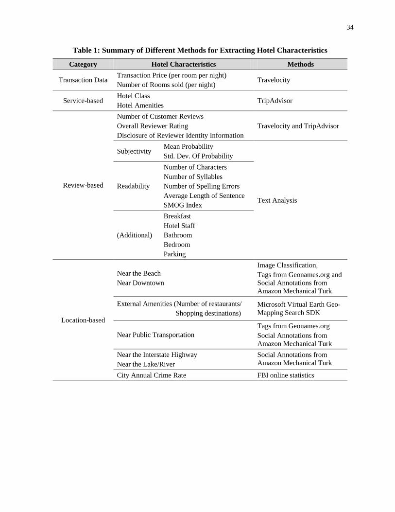
34

Table 1: Summary of Different Methods for Extracting Hotel Characteristics

Category Hotel Characteristics Methods

Transaction Data Transaction Price (per room per night)

Number of Rooms sold (per night) Travelocity

Service-based Hotel Class

Hotel Amenities TripAdvisor

Review-based

Number of Customer Reviews

Overall Reviewer Rating

Disclosure of Reviewer Identity Information

Travelocity and TripAdvisor

Subjectivity Mean Probability

Std. Dev. Of Probability

Text Analysis

Readability

Number of Characters

Number of Syllables

Number of Spelling Errors

Average Length of Sentence

SMOG Index

(Additional)

Breakfast

Hotel Staff

Bathroom

Bedroom

Parking

Location-based

Near the Beach

Near Downtown

Image Classification,

Tags from Geonames.org and

Social Annotations from

Amazon Mechanical Turk

External Amenities (Number of restaurants/

Shopping destinations)

Microsoft Virtual Earth Geo-

Mapping Search SDK

Near Public Transportation

Tags from Geonames.org

Social Annotations from

Amazon Mechanical Turk

Near the Interstate Highway

Near the Lake/River

Social Annotations from

Amazon Mechanical Turk

City Annual Crime Rate FBI online statistics

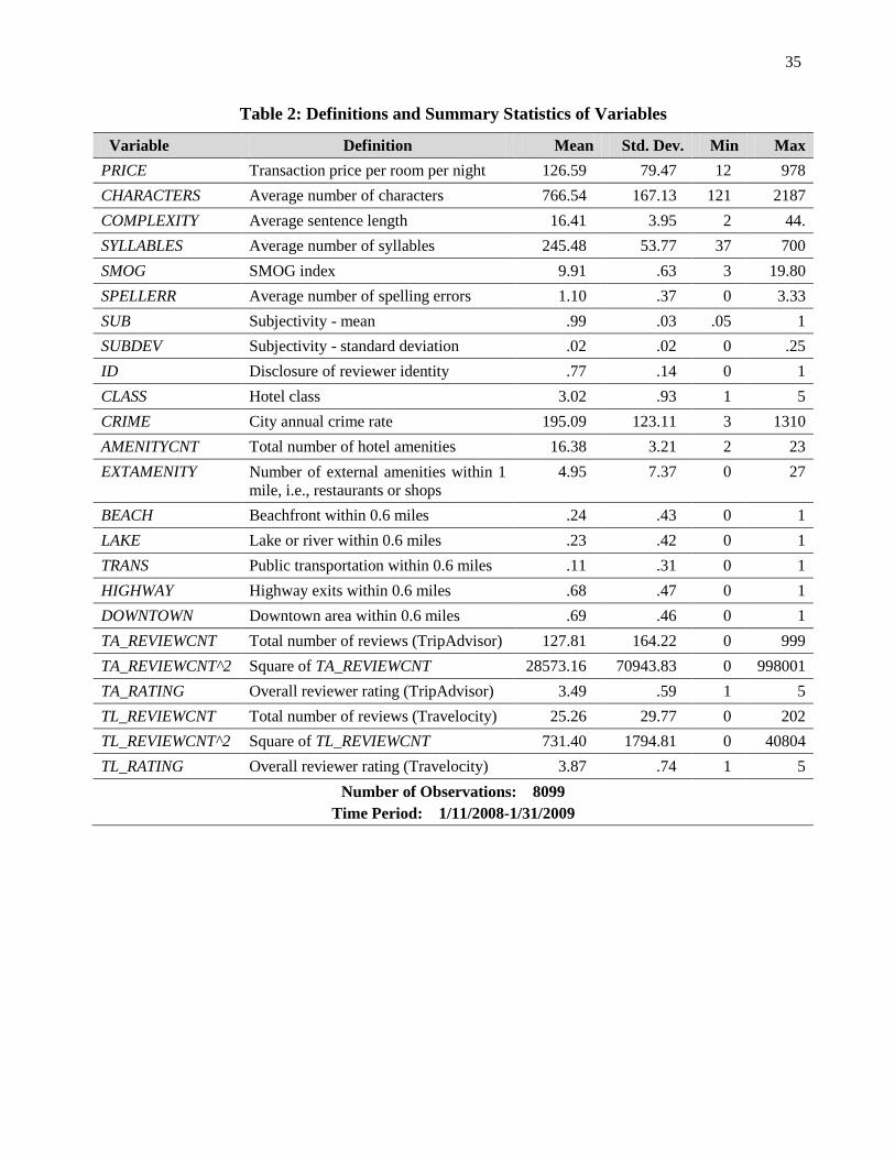
35

Table 2: Definitions and Summary Statistics of Variables

Variable Definition Mean Std. Dev. Min Max

PRICE Transaction price per room per night 126.59 79.47 12 978

CHARACTERS Average number of characters 766.54 167.13 121 2187

COMPLEXITY Average sentence length 16.41 3.95 2 44.

SYLLABLES Average number of syllables 245.48 53.77 37 700

SMOG SMOG index 9.91 .63 3 19.80

SPELLERR Average number of spelling errors 1.10 .37 0 3.33

SUB Subjectivity - mean .99 .03 .05 1

SUBDEV Subjectivity - standard deviation .02 .02 0 .25

ID Disclosure of reviewer identity .77 .14 0 1

CLASS Hotel class 3.02 .93 1 5

CRIME City annual crime rate 195.09 123.11 3 1310

AMENITYCNT Total number of hotel amenities 16.38 3.21 2 23

EXTAMENITY Number of external amenities within 1

mile, i.e., restaurants or shops

4.95 7.37 0 27

BEACH Beachfront within 0.6 miles .24 .43 0 1

LAKE Lake or river within 0.6 miles .23 .42 0 1

TRANS Public transportation within 0.6 miles .11 .31 0 1

HIGHWAY Highway exits within 0.6 miles .68 .47 0 1

DOWNTOWN Downtown area within 0.6 miles .69 .46 0 1

TA_REVIEWCNT Total number of reviews (TripAdvisor) 127.81 164.22 0 999

TA_REVIEWCNT^2 Square of TA_REVIEWCNT 28573.16 70943.83 0 998001

TA_RATING Overall reviewer rating (TripAdvisor) 3.49 .59 1 5

TL_REVIEWCNT Total number of reviews (Travelocity) 25.26 29.77 0 202

TL_REVIEWCNT^2 Square of TL_REVIEWCNT 731.40 1794.81 0 40804

TL_RATING Overall reviewer rating (Travelocity) 3.87 .74 1 5

Number of Observations: 8099

Time Period: 1/11/2008-1/31/2009

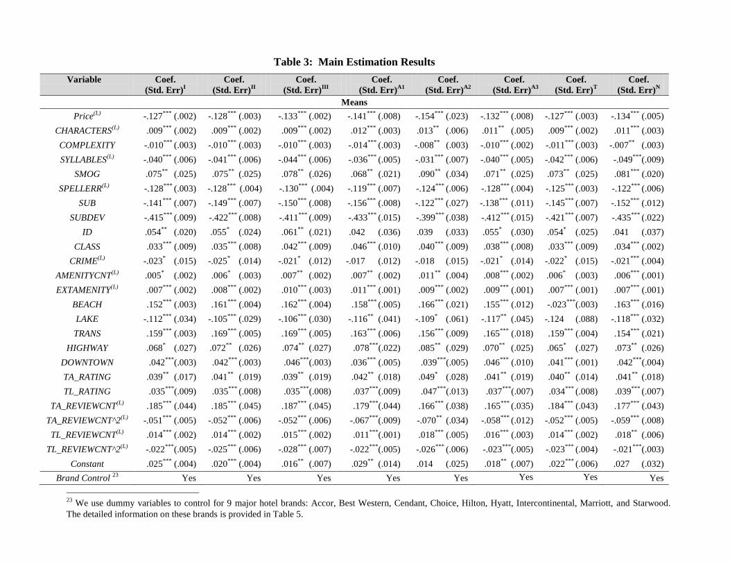
Table 3: Main Estimation Results

Variable Coef.

(Std. Err)I

Coef.

(Std. Err)II

Coef.

(Std. Err)III

Coef.

(Std. Err)A1

Coef.

(Std. Err)A2

Coef.

(Std. Err)A3

Coef.

(Std. Err)T

Coef.

(Std. Err)N

Means

Price(L)

-.127***

(.002) -.128***

(.003) -.133***

(.002) -.141***

(.008) -.154***

(.023) -.132***

(.008) -.127***

(.003) -.134***

(.005)

CHARACTERS(L)

.009***

(.002) .009***

(.002) .009***

(.002) .012***

(.003) .013**

(.006) .011**

(.005) .009***

(.002) .011***

(.003)

COMPLEXITY -.010***

(.003) -.010***

(.003) -.010***

(.003) -.014***

(.003) -.008**

(.003) -.010***

(.002) -.011***

(.003) -.007**

(.003)

SYLLABLES(L)

-.040***

(.006) -.041***

(.006) -.044***

(.006) -.036***

(.005) -.031***

(.007) -.040***

(.005) -.042***

(.006) -.049***

(.009)

SMOG .075**

(.025) .075**

(.025) .078**

(.026) .068**

(.021) .090**

(.034) .071**

(.025) .073**

(.025) .081***

(.020)

SPELLERR(L)

-.128***

(.003) -.128***

(.004) -.130***

(.004) -.119***

(.007) -.124***

(.006) -.128***

(.004) -.125***

(.003) -.122***

(.006)

SUB -.141***

(.007) -.149***

(.007) -.150***

(.008) -.156***

(.008) -.122***

(.027) -.138***

(.011) -.145***

(.007) -.152***

(.012)

SUBDEV -.415***

(.009) -.422***

(.008) -.411***

(.009) -.433***

(.015) -.399***

(.038) -.412***

(.015) -.421***

(.007) -.435***

(.022)

ID .054**

(.020) .055* (.024) .061

** (.021) .042

(.036) .039

(.033) .055

* (.030) .054

* (.025) .041

(.037)

CLASS .033***

(.009) .035***

(.008) .042***

(.009) .046***

(.010) .040***

(.009) .038***

(.008) .033***

(.009) .034***

(.002)

CRIME(L)

-.023*

(.015) -.025* (.014) -.021

* (.012) -.017

(.012) -.018

(.015) -.021

* (.014) -.022

* (.015) -.021

*** (.004)

AMENITYCNT(L)

.005*

(.002) .006*

(.003) .007**

(.002) .007**

(.002) .011**

(.004) .008***

(.002) .006*

(.003) .006***

(.001)

EXTAMENITY(L)

.007***

(.002) .008***

(.002) .010***

(.003) .011***

(.001) .009***

(.002) .009***

(.001) .007***

(.001) .007***

(.001)

BEACH .152***

(.003) .161***

(.004) .162***

(.004) .158***

(.005) .166***

(.021) .155***

(.012) -.023***

(.003) .163***

(.016)

LAKE -.112***

(.034) -.105***

(.029) -.106***

(.030) -.116**

(.041) -.109*

(.061) -.117**

(.045) -.124 (.088) -.118***

(.032)

TRANS .159***

(.003) .169***

(.005) .169***

(.005) .163***

(.006) .156***

(.009) .165***

(.018) .159***

(.004) .154***

(.021)

HIGHWAY .068* (.027) .072

** (.026) .074

** (.027) .078

***(.022) .085

** (.029) .070

** (.025) .065

* (.027) .073

** (.026)

DOWNTOWN .042***

(.003) .042***

(.003) .046***

(.003) .036***

(.005) .039***

(.005) .046***

(.010) .041***

(.001) .042***

(.004)

TA_RATING .039**

(.017) .041**

(.019) .039**

(.019) .042**

(.018) .049*

(.028) .041**

(.019) .040**

(.014) .041**

(.018)

TL_RATING .035***

(.009) .035***

(.008) .035***

(.008) .037***

(.009) .047***

(.013) .037***

(.007) .034***

(.008) .039***

(.007)

TA_REVIEWCNT(L)

.185***

(.044) .185***

(.045) .187***

(.045) .179***

(.044) .166***

(.038) .165***

(.035) .184***

(.043) .177***

(.043)

TA_REVIEWCNT^2(L)

-.051***

(.005) -.052***

(.006) -.052***

(.006) -.067***

(.009) -.070**

(.034) -.058***

(.012) -.052***

(.005) -.059***

(.008)

TL_REVIEWCNT(L)

.014***

(.002) .014***

(.002) .015***

(.002) .011***

(.001) .018***

(.005) .016***

(.003) .014***

(.002) .018**

(.006)

TL_REVIEWCNT^2(L)

-.022***

(.005) -.025***

(.006) -.028***

(.007) -.022***

(.005) -.026***

(.006) -.023***

(.005) -.023***

(.004) -.021***

(.003)

Constant .025***

(.004) .020***

(.004) .016**

(.007) .029**

(.014) .014 (.025) .018

** (.007) .022

*** (.006) .027

(.032)

Brand Control 23

Yes Yes Yes Yes Yes Yes Yes Yes

23

We use dummy variables to control for 9 major hotel brands: Accor, Best Western, Cendant, Choice, Hilton, Hyatt, Intercontinental, Marriott, and Starwood.

The detailed information on these brands is provided in Table 5.

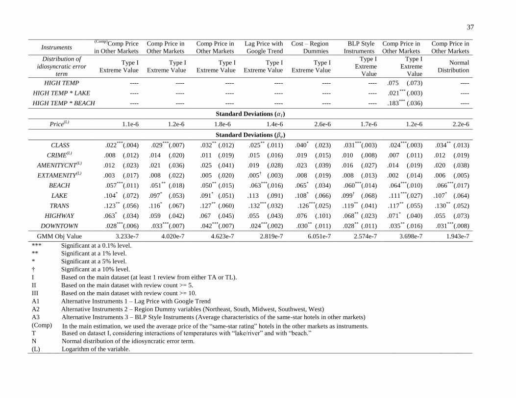
37

Instruments (Comp)

Comp Price

in Other Markets

Comp Price in

Other Markets

Comp Price in

Other Markets

Lag Price with

Google Trend

Cost – Region

Dummies

BLP Style

Instruments

Comp Price in

Other Markets

Comp Price in

Other Markets

Distribution of

idiosyncratic error

term

Type I

Extreme Value

Type I

Extreme Value

Type I

Extreme Value

Type I

Extreme Value

Type I

Extreme Value

Type I

Extreme

Value

Type I

Extreme

Value

Normal

Distribution

HIGH TEMP ---- ---- ---- ---- ---- ---- .075 (.073) ----

HIGH TEMP * LAKE ---- ---- ---- ---- ---- ---- .021***

(.003) ----

HIGH TEMP * BEACH ---- ---- ---- ---- ---- ---- .183***

(.036) ----

Standard Deviations ( )

Price(L)

1.1e-6 1.2e-6 1.8e-6 1.4e-6 2.6e-6 1.7e-6 1.2e-6 2.2e-6

Standard Deviations ( )

CLASS .022***

(.004) .029***

(.007) .032**

(.012) .025**

(.011) .040* (.023) .031

***(.003) .024

***(.003) .034

** (.013)

CRIME(L)

.008

(.012) .014 (.020) .011 (.019) .015

(.016) .019 (.015) .010 (.008) .007

(.011) .012 (.019)

AMENITYCNT(L)

.012 (.023) .021 (.036) .025 (.041) .019 (.028) .023 (.039) .016 (.027) .014 (.019) .020 (.038)

EXTAMENITY(L)

.003 (.017) .008 (.022) .005 (.020) .005

† (.003) .008 (.019) .008

(.013) .002 (.014) .006 (.005)

BEACH

.057***

(.011) .051**

(.018) .050**

(.015) .063***

(.016) .065* (.034) .060

***(.014) .064

***(.010) .066

***(.017)

LAKE

.104*

(.072) .097* (.053) .091

* (.051) .113

(.091) .108

* (.066) .099

† (.068) .111

***(.027) .107

* (.064)

TRANS

.123**

(.056) .116* (.067) .127

** (.060) .132

*** (.032) .126

***(.025) .119

** (.041) .117

** (.055) .130

** (.052)

HIGHWAY

.063* (.034) .059 (.042) .067

(.045) .055

(.043) .076 (.101) .068

** (.023) .071

* (.040) .055 (.073)

DOWNTOWN

.028***

(.006) .033***

(.007) .042***

(.007) .024***

(.002) .030**

(.011) .028**

(.011) .035**

(.016) .031***

(.008)

GMM Obj Value 3.233e-7 4.020e-7 4.623e-7 2.819e-7 6.051e-7 2.574e-7 3.698e-7 1.943e-7

*** Significant at a 0.1% level. ** Significant at a 1% level. * Significant at a 5% level. † Significant at a 10% level. I Based on the main dataset (at least 1 review from either TA or TL). II Based on the main dataset with review count >= 5. III Based on the main dataset with review count >= 10. A1 Alternative Instruments 1 – Lag Price with Google Trend A2 Alternative Instruments 2 – Region Dummy variables (Northeast, South, Midwest, Southwest, West) A3 Alternative Instruments 3 – BLP Style Instruments (Average characteristics of the same-star hotels in other markets) (Comp) In the main estimation, we used the average price of the “same-star rating” hotels in the other markets as instruments. T Based on dataset I, considering interactions of temperatures with “lake/river” and with “beach.” N Normal distribution of the idiosyncratic error term. (L) Logarithm of the variable.

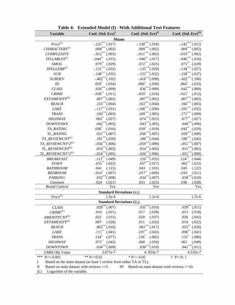
Table 4: Extended Model (I) –With Additional Text Features

Variable Coef. (Std. Err)I

Coef. (Std. Err)II

Coef. (Std. Err)III

Means

Price(L)

-.125***

(.017) -.130***

(.018) -.142***

(.012)

CHARACTERS(L)

.008***

(.002) .009***

(.002) .009***

(.002)

COMPLEXITY -.012***

(.003) -.011***

(.002) -.010***

(.002)

SYLLABLES(L)

-.044**

(.015) -.040**

(.017) -.046***

(.016)

SMOG .079**

(.029) .072**

(.025) .071**

(.029)

SPELLERR(L)

-.131***

(.032) -.135***

(.029) -.138***

(.027)

SUB -.148***

(.035) -.152***

(.032) -.158***

(.037)

SUBDEV -.402***

(.102) -.418***

(.099) -.422***

(.106)

ID .059* (.034) .060

* (.030) .064

* (.033)

CLASS .036***

(.009) .036***

(.009) .042***

(.009)

CRIME -.030**

(.011) -.029*

(.016) -.021*

(.012)

EXTAMENITY(L)

.007***

(.002) .007***

(.002) .007***

(.002)

BEACH .153***

(.004) .163***

(.004) .166***

(.005)

LAKE -.117***

(.031) -.108***

(.030) -.105***

(.032)

TRANS .160***

(.003) .169***

(.005) .171***

(.008)

HIGHWAY .063* (.027) .074

***(.023) .077

** (.027)

DOWNTOWN .042***

(.005) .043***

(.005) .049***

(.006)

TA_RATING .036*

(.016) .039*

(.019) .042**

(.020)

TL_RATING .031***

(.007) .036***

(.007) .039***

(.009)

TA_REVIEWCNT(L)

.181***

(.039) .186***

(.044) .188***

(.045)

TA_REVIEWCNT^2(L)

-.056***

(.006) -.059***

(.009) -.051***

(.007)

TL_REVIEWCNT(L)

.016***

(.002) .014***

(.002) .015***

(.002)

TL_REVIEWCNT^2(L)

-.024***

(.005) -.026***

(.006) -.031***

(.009)

BREAKFAST .112**

(.049) .120***

(.035) .124**

(.044)

STAFF .055**

(.022) .057***

(.017) .062**

(.023)

BATHROOM .041 (.115) .043

(.101) .045

(.122)

BEDROOM -.014*

(.007) -.017† (.009) -.010

(.011)

PARKING .032***

(.008) .034***

(.007) .039***

(.010)

Constant . 024

(.021) .031 (.025) .036 (.028)

Brand Control Yes Yes Yes

Standard Deviations ( )

Price(L)

1.5e-6 1.1e-6 1.7e-6

Standard Deviations ( )

CLASS

.028***

(.007) .035***

(.010) .039**

(.011)

CRIME(L)

.010

(.021) .017 (.028) .013 (.018)

AMENITYCNT(L)

.022 (.031) .020 (.037) .026 (.042)

EXTAMENITY(L)

.007 (.026) .011 (.032) .014 (.022)

BEACH

.063***

(.016) .061***

(.017) .055**

(.020)

LAKE

.111**

(.041) .107**

(.043) .098**

(.041)

TRANS

.134*

(.077) .136* (.082) .131

* (.080)

HIGHWAY

.072* (.042) .068 (.050) .061

(.049)

DOWNTOWN

.034***

(.009) .038***

(.010) .041***

(.011)

GMM Obj Value 3.671e-7 4. 823e-7 4.535e-7

*** P<= 0.001 ** P<=0.01 * P<= 0.05 † P<=0. 1

I Based on the main dataset (at least 1 review from either TA or TL).

II Based on main dataset with reviews >=5. III Based on main dataset with reviews >=10.

(L) Logarithm of the variable.

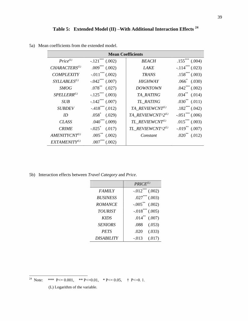
39

Table 5: Extended Model (II) –With Additional Interaction Effects 24

5a) Mean coefficients from the extended model.

Mean Coefficients

Price(L) -.121***

(.002) BEACH .155***

(.004)

CHARACTERS(L) .009***

(.002) LAKE -.114***

(.023)

COMPLEXITY -.011***

(.002) TRANS .158***

(.003)

SYLLABLES(L) -.042***

(.007) HIGHWAY .066* (.030)

SMOG .078**

(.027) DOWNTOWN .042***

(.002)

SPELLERR(L) -.125***

(.003) TA_RATING .034**

(.014)

SUB -.142***

(.007) TL_RATING .030**

(.011)

SUBDEV -.418***

(.012) TA_REVIEWCNT(L) .182***

(.042)

ID .058* (.029) TA_REVIEWCNT^2(L) -.051

*** (.006)

CLASS .040***

(.009) TL_REVIEWCNT(L) .015***

(.003)

CRIME -.025* (.017) TL_REVIEWCNT^2(L) -.019

** (.007)

AMENITYCNT(L) .005**

(.002) Constant .020**

(.012)

EXTAMENITY(L) .007***

(.002)

5b) Interaction effects between Travel Category and Price.

PRICE(L)

FAMILY -.012***

(.002)

BUSINESS .027***

(.003)

ROMANCE -.005**

(.002)

TOURIST -.018***

(.005)

KIDS .014**

(.007)

SENIORS .088 (.053)

PETS .020 (.033)

DISABILITY -.013 (.017)

24

Note: *** P<= 0.001, ** P<=0.01, * P<= 0.05, † P<=0. 1.

(L) Logarithm of the variable.

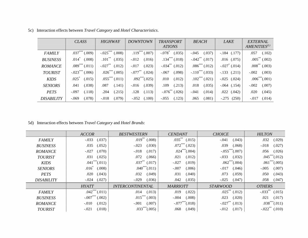
5c) Interaction effects between Travel Category and Hotel Characteristics.

CLASS

HIGHWAY DOWNTOWN TRANSPORT

ATIONS

BEACH LAKE EXTERNAL

AMENITIES(L)

FAMILY .037***

(.009) -.025***

(.008) .119***

(.007) -.078* (.035) -.045 (.037) -.184 (.177) .057 (.102)

BUSINESS .014*

(.008) .101**

(.035) -.012 (.016) .134***

(.018) -.042**

(.017) .016 (.075) .005**

(.002)

ROMANCE .089***

(.011) -.027**

(.012) -.017 (.023) -.034**

(.012) .086***

(.012) -.027*

(.014) .008**

(.003)

TOURIST -.023***

(.006) .026***

(.005) -.077**

(.024) -.067 (.098) -.110

*** (.033) -.133 (.211) -.002 (.003)

KIDS .025* (.015) .055

*** (.011) .092

***(.025) .010 (.012) .102

*** (.021) -.025 (.024) .006

***(.001)

SENIORS .041 (.038) .087

(.141) -.016

(.039) .109

(.213) .018

(.035) -.064

(.154) -.002

(.007)

PETS -.097 (.118) .204 (.215) .128 (.113) -.076**

(.026) -.041 (.014) .022 (.042) .020 (.045)

DISABILITY -.069 (.078) -.018 (.079) -.052 (.100) -.055 (.123) .065 (.081) -.275 (250) -.017 (.014)

5d) Interaction effects between Travel Category and Hotel Brands:

ACCOR

BESTWESTERN CENDANT CHOICE HILTON

FAMILY -.033 (.037) .019**

(.008) .035**

(.015) -.041 (.043) .032 (.029)

BUSINESS .035 (.052) -.023 (.030) .072***

(.023) .039 (.068) -.018 (.027)

ROMANCE -.027 (.070) -.018 (.017) .024***

(.004) -.055***

(.007) .056 (.026)

TOURIST .031 (.025) .072 (.066) .021 (.012) -.033 (.032) .045***

(.012)

KIDS .041***

(.011) .037**

(.017) -.027 (.019) .062***

(.004) .061***

(.005)

SENIORS .016* (.008) .040

***(.011) -.007 (.006) -.017

(.046) -.005 (.007)

PETS .020 (.043) .032 (.049) .031 (.040) .073 (.059) .050 (.043)

DISABILITY -.024 (.027) -.029 (.036) .042 (.035) -.025 (.047) .058 (.047)

HYATT

INTERCONTINENTAL MARRIOTT STARWOOD OTHERS

FAMILY .042***

(.011) .014 (.013) .019 (.022) .025**

(.012) -.033**

(.015)

BUSINESS -.007***

(.002) .015***

(.003) -.004 (.008) .023 (.020) .021 (.017)

ROMANCE -.010 (.012) -.001 (.007) -.077***

(.018) -.027**

(.013) .038***

(.011)

TOURIST -.021 (.018) .033***

(.005) .068 (.049) -.012 (.017) -.022**

(.010)

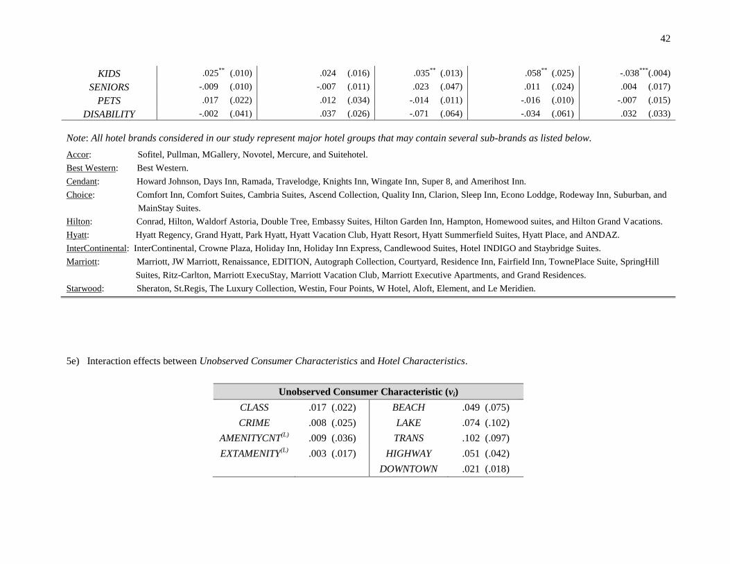
42

KIDS .025**

(.010) .024 (.016) .035**

(.013) .058**

(.025) -.038***

(.004)

SENIORS -.009 (.010) -.007 (.011) .023 (.047) .011 (.024) .004 (.017)

PETS .017 (.022) .012 (.034) -.014 (.011) -.016 (.010) -.007 (.015)

DISABILITY -.002 (.041) .037 (.026) -.071 (.064) -.034 (.061) .032 (.033)

Note: All hotel brands considered in our study represent major hotel groups that may contain several sub-brands as listed below.

Accor: Sofitel, Pullman, MGallery, Novotel, Mercure, and Suitehotel.

Best Western: Best Western.

Cendant: Howard Johnson, Days Inn, Ramada, Travelodge, Knights Inn, Wingate Inn, Super 8, and Amerihost Inn.

Choice: Comfort Inn, Comfort Suites, Cambria Suites, Ascend Collection, Quality Inn, Clarion, Sleep Inn, Econo Loddge, Rodeway Inn, Suburban, and

MainStay Suites.

Hilton: Conrad, Hilton, Waldorf Astoria, Double Tree, Embassy Suites, Hilton Garden Inn, Hampton, Homewood suites, and Hilton Grand Vacations.

Hyatt: Hyatt Regency, Grand Hyatt, Park Hyatt, Hyatt Vacation Club, Hyatt Resort, Hyatt Summerfield Suites, Hyatt Place, and ANDAZ.

InterContinental: InterContinental, Crowne Plaza, Holiday Inn, Holiday Inn Express, Candlewood Suites, Hotel INDIGO and Staybridge Suites.

Marriott: Marriott, JW Marriott, Renaissance, EDITION, Autograph Collection, Courtyard, Residence Inn, Fairfield Inn, TownePlace Suite, SpringHill

Suites, Ritz-Carlton, Marriott ExecuStay, Marriott Vacation Club, Marriott Executive Apartments, and Grand Residences.

Starwood: Sheraton, St.Regis, The Luxury Collection, Westin, Four Points, W Hotel, Aloft, Element, and Le Meridien.

5e) Interaction effects between Unobserved Consumer Characteristics and Hotel Characteristics.

Unobserved Consumer Characteristic (vi)

CLASS .017 (.022) BEACH .049 (.075)

CRIME .008 (.025) LAKE .074 (.102)

AMENITYCNT(L)

.009 (.036) TRANS .102 (.097)

EXTAMENITY(L)

.003 (.017) HIGHWAY .051 (.042)

DOWNTOWN .021 (.018)

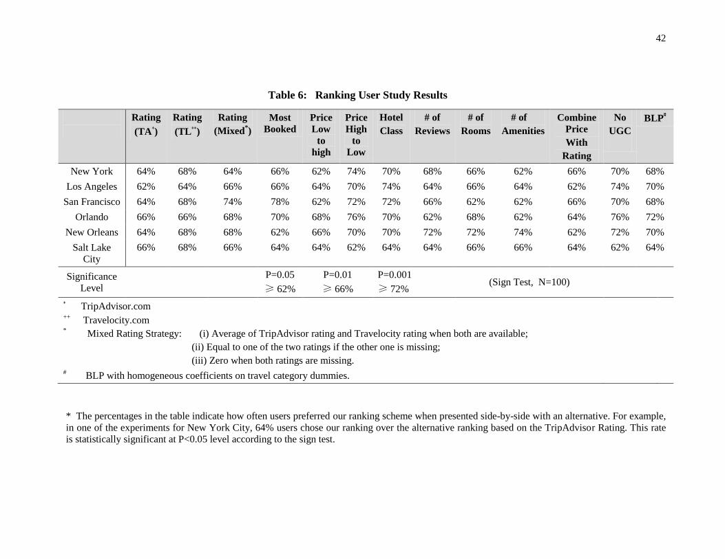
42

Table 6: Ranking User Study Results

Rating

(TA+)

Rating

(TL++

)

Rating

(Mixed*)

Most

Booked

Price

Low

to

high

Price

High

to

Low

Hotel

Class

# of

Reviews

# of

Rooms

# of

Amenities

Combine

Price

With

Rating

No

UGC

BLP#

New York 64% 68% 64% 66% 62% 74% 70% 68% 66% 62% 66% 70% 68%

Los Angeles 62% 64% 66% 66% 64% 70% 74% 64% 66% 64% 62% 74% 70%

San Francisco 64% 68% 74% 78% 62% 72% 72% 66% 62% 62% 66% 70% 68%

Orlando 66% 66% 68% 70% 68% 76% 70% 62% 68% 62% 64% 76% 72%

New Orleans 64% 68% 68% 62% 66% 70% 70% 72% 72% 74% 62% 72% 70%

Salt Lake

City

66% 68% 66% 64% 64% 62% 64% 64% 66% 66% 64% 62% 64%

Significance

Level

P=0.05

≥ 62%

P=0.01

≥ 66%

P=0.001

≥ 72% (Sign Test, N=100)

+ TripAdvisor.com

++ Travelocity.com

* Mixed Rating Strategy: (i) Average of TripAdvisor rating and Travelocity rating when both are available;

(ii) Equal to one of the two ratings if the other one is missing;

(iii) Zero when both ratings are missing.

# BLP with homogeneous coefficients on travel category dummies.

* The percentages in the table indicate how often users preferred our ranking scheme when presented side-by-side with an alternative. For example,

in one of the experiments for New York City, 64% users chose our ranking over the alternative ranking based on the TripAdvisor Rating. This rate

is statistically significant at P<0.05 level according to the sign test.

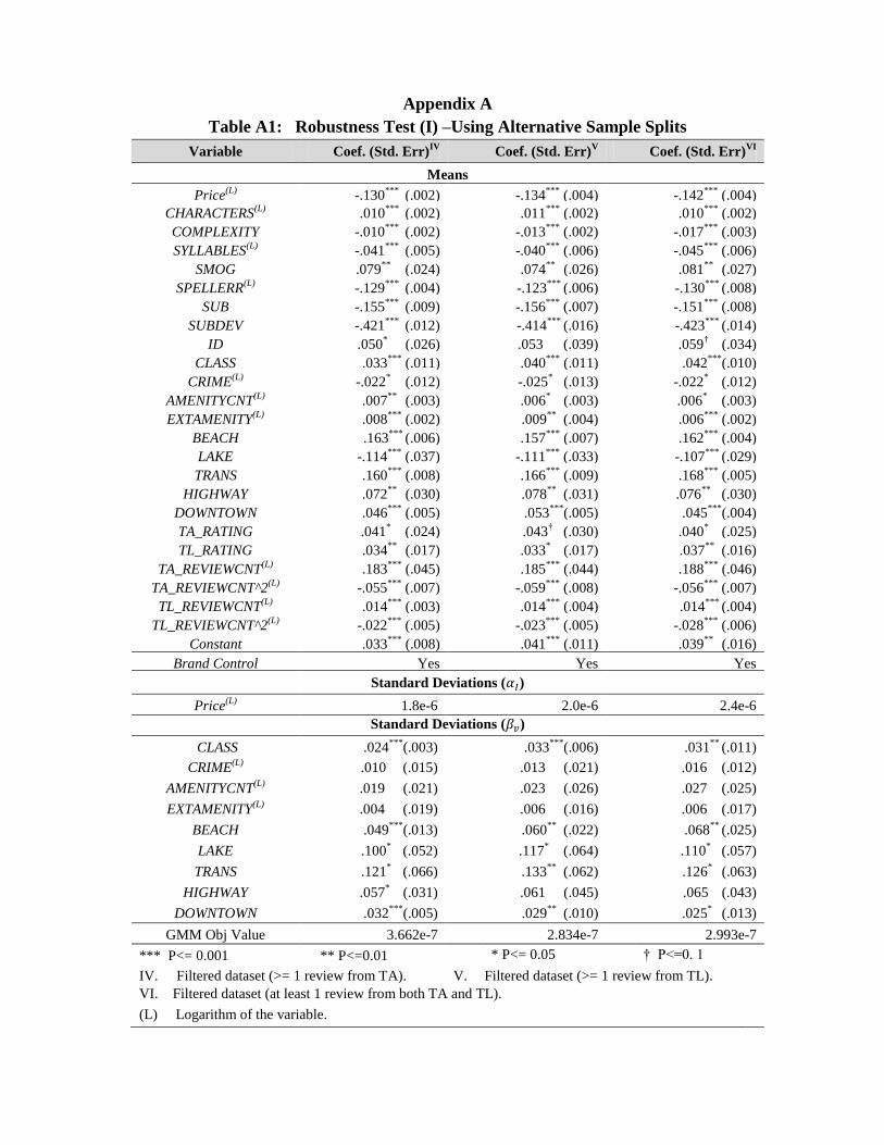
Appendix A

Table A1: Robustness Test (I) –Using Alternative Sample Splits

Variable Coef. (Std. Err)IV

Coef. (Std. Err)V Coef. (Std. Err)

VI

Means

Price(L)

-.130***

(.002) -.134***

(.004) -.142***

(.004)

CHARACTERS(L)

.010***

(.002) .011***

(.002) .010***

(.002)

COMPLEXITY -.010***

(.002) -.013***

(.002) -.017***

(.003)

SYLLABLES(L)

-.041***

(.005) -.040***

(.006) -.045***

(.006)

SMOG .079**

(.024) .074**

(.026) .081**

(.027)

SPELLERR(L)

-.129***

(.004) -.123***

(.006) -.130***

(.008)

SUB -.155***

(.009) -.156***

(.007) -.151***

(.008)

SUBDEV -.421***

(.012) -.414***

(.016) -.423***

(.014)

ID .050*

(.026) .053

(.039) .059† (.034)

CLASS .033***

(.011) .040***

(.011) .042***

(.010)

CRIME(L)

-.022* (.012) -.025

* (.013) -.022

* (.012)

AMENITYCNT(L)

.007**

(.003) .006*

(.003) .006*

(.003)

EXTAMENITY(L)

.008***

(.002) .009**

(.004) .006***

(.002)

BEACH .163***

(.006) .157***

(.007) .162***

(.004)

LAKE -.114***

(.037) -.111***

(.033) -.107***

(.029)

TRANS .160***

(.008) .166***

(.009) .168***

(.005)

HIGHWAY .072**

(.030) .078**

(.031) .076**

(.030)

DOWNTOWN .046***

(.005) .053***

(.005) .045***

(.004)

TA_RATING .041*

(.024) .043†

(.030) .040*

(.025)

TL_RATING .034**

(.017) .033*

(.017) .037**

(.016)

TA_REVIEWCNT(L)

.183***

(.045) .185***

(.044) .188***

(.046)

TA_REVIEWCNT^2(L)

-.055***

(.007) -.059***

(.008) -.056***

(.007)

TL_REVIEWCNT(L)

.014***

(.003) .014***

(.004) .014***

(.004)

TL_REVIEWCNT^2(L)

-.022***

(.005) -.023***

(.005) -.028***

(.006)

Constant .033***

(.008) .041***

(.011) .039**

(.016)

Brand Control Yes Yes Yes

Standard Deviations ( )

Price(L)

1.8e-6 2.0e-6 2.4e-6

Standard Deviations ( )

CLASS

.024***

(.003) .033***

(.006) .031**

(.011)

CRIME(L)

.010

(.015) .013 (.021) .016 (.012)

AMENITYCNT(L)

.019 (.021) .023 (.026) .027 (.025)

EXTAMENITY(L)

.004 (.019) .006 (.016) .006 (.017)

BEACH

.049***

(.013) .060**

(.022) .068**

(.025)

LAKE

.100*

(.052) .117* (.064) .110

* (.057)

TRANS

.121*

(.066) .133**

(.062) .126*

(.063)

HIGHWAY

.057* (.031) .061 (.045) .065

(.043)

DOWNTOWN

.032***

(.005) .029**

(.010) .025* (.013)

GMM Obj Value 3.662e-7 2.834e-7 2.993e-7

*** P<= 0.001 ** P<=0.01 * P<= 0.05 † P<=0. 1

IV. Filtered dataset (>= 1 review from TA). V. Filtered dataset (>= 1 review from TL).

VI. Filtered dataset (at least 1 review from both TA and TL).

(L) Logarithm of the variable.

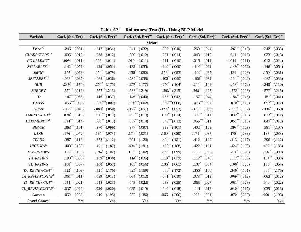
Table A2: Robustness Test (II) - Using BLP Model

Variable Coef. (Std. Err)I

Coef. (Std. Err)II

Coef. (Std. Err)III

Coef. (Std. Err)IV

Coef. (Std. Err)V

Coef. (Std. Err)VI

Coef. (Std. Err) R

Means

Price(L)

-.246***

(.031) -.247***

(.034) -.241***

(.032) -.252***

(.040) -.260***

(.044) -.261***

(.042) -.242***

(.033)

CHARACTERS(L)

.035**

(.012) .038***

(.012) .039***

(.012) .031**

(.014) .043**

(.015) .041**

(.016) .033**

(.013)

COMPLEXITY -.009 (.011) -.009

(.011) -.010

(.011) -.011

(.010) -.016

(.011) -.014

(.011) -.012

(.014)

SYLLABLES(L)

-.142**

(.052) -.139**

(.051) -.132**

(.055) -.140**

(.060) -.146**

(.061) -.149**

(.062) -.146**

(.054)

SMOG .157*

(.078) .154*

(.079) .156*

(.080) .158*

(.093) .142*

(.095) .134†

(.103) .150*

(.081)

SPELLERR(L)

-.089**

(.035) -.092**

(.036) -.096**

(.038) -.102**

(.040) -.106**

(.039) -.104**

(.040) -.095**

(.038)

SUB -.249* (.174) -.253

* (.175) -.257

* (.177) -.250

* (.164) -.266

* (.169) -.269

* (.172) -.240

* (.110)

SUBDEV -.570**

(.212) -.577**

(.215) -.583**

(.219) -.593**

(.215) -.568**

(.207) -.572**

(.208) -.577**

(.215)

ID .147***

(.036) .146***

(.037) .146***

(.040) .153***

(.042) .157***

(.044) .154***

(.046) .151***

(.041)

CLASS .055***

(.002) .056***

(.002) .056***

(.002) .062***

(.006) .073***

(.007) .070***

(.010) .057***

(.012)

CRIME -.088*

(.049) -.089*

(.050) -.086*

(.051) -.095*

(.053) -.100*

(.056) -.099*

(.057) -.094*

(.050)

AMENITYCNT(L)

.028*

(.015) .031**

(.014) .033**

(.014) .037**

(.014) .038**

(.014) .032**

(.013) .032**

(.012)

EXTAMENITY(L)

.034**

(.014) .036**

(.013) .037**

(.014) .043***

(.012) .055***

(.011) .051***

(.010) .047***

(.012)

BEACH .363***

(.101) .370***

(.099) .377***

(.097) .383***

(.101) .402***

(.102) .394***

(.103) .381***

(.107)

LAKE -.176**

(.072) -.167**

(.074) -.170**

(.071) -.169**

(.080) -.174**

(.087) -.178**

(.083) -.167**

(.083)

TRANS .387***

(.113) .382***

(.112) .391***

(.120) .404***

(.121) .412***

(.120) .413***

(.117) .396***

(.112)

HIGHWAY .403**

(.186) .401**

(.187) .404**

(.191) .408**

(.188) .422**

(.191) .424**

(.193) .407**

(.185)

DOWNTOWN .192*

(.105) .194*

(.102) .188*

(.102) .202*

(.099) .205*

(.099) .201*

(.098) .197*

(.099)

TA_RATING .103**

(.039) .109**

(.038) .114**

(.035) .119**

(.039) .117**

(.040) .117**

(.038) .104**

(.030)

TL_RATING .108*

(.057) .108*

(.057) .105*

(.056) .106*

(.061) .107*

(.054) .108*

(.055) .108*

(.054)

TA_REVIEWCNT(L)

.322*

(.169) .321*

(.170) .325*

(.169) .333*

(.172) .356*

(.186) .349*

(.181) .336*

(.176)

TA_REVIEWCNT^2(L)

-.061***

(.011) -.059***

(.013) -.064***

(.012) -.071***

(.010) -.078***

(.012) -.069***

(.012) -.062***

(.012)

TL_REVIEWCNT(L)

.044**

(.021) .048**

(.023) .045**

(.022) .053**

(.025) .065**

(.027) .061**

(.026) .049**

(.022)

TL_REVIEWCNT^2(L)

-.037*

(.020) -.036* (.020) -.035

* (.019) -.040

** (.018) -.041

** (.018) -.040

** (.017) -.039

** (.016)

Constant .052 (.203) .046

(.195) .057

(.186) .066

(.206) .069

(.201) .070

(.203) .060

(.198)

Brand Control Yes Yes Yes Yes Yes Yes Yes

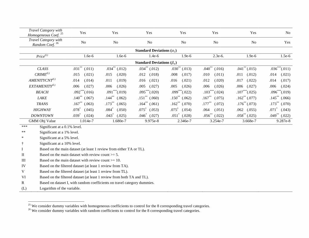
Travel Category with

Homogeneous Coef. 25

Yes Yes Yes Yes Yes Yes No

Travel Category with

Random Coef. 26

No No No No No No Yes

Standard Deviations ( )

Price(L)

1.6e-6 1.6e-6 1.4e-6 1.9e-6 2.3e-6. 1.9e-6 1.5e-6

Standard Deviations ( )

CLASS

.031**

(.011) .034**

(.012) .034**

(.012) .030**

(.013) .040**

(.016) .041**

(.015) .036***

(.011)

CRIME(L)

.015

(.021) .015 (.020) .012 (.018) .008

(.017) .010 (.011) .011 (.012) .014

(.021)

AMENITYCNT(L)

.014 (.014) .011 (.019) .016 (.021) .016 (.021) .012 (.020) .017 (.022) .014 (.017)

EXTAMENITY(L)

.006 (.027) .006 (.026) .005 (.027) .005 (.026) .006 (.026) .006 (.027) .006 (.024)

BEACH

.092***

(.016) .091***

(.019) .095***

(.020) .099***

(.022) .103***

(.024) .107***

(.025) .096***

(.019)

LAKE

.140**

(.067) .144**

(.062) .151**

(.060) .150**

(.062) .167**

(.075) .162**

(.077) .145**

(.066)

TRANS

.167**

(.063) .173**

(.065) .164**

(.061) .162**

(.070) .177**

(.072) .176**

(.073) .173**

(.070)

HIGHWAY

.078* (.045) .084

* (.050) .075

† (.053) .075

† (.054) .064 (.051) .062

(.055) .071

* (.043)

DOWNTOWN .039* (.024) .043

* (.025) .046

* (.027) .051

* (.028) .056

** (.022) .058

** (.025) .049

** (.022)

GMM Obj Value 1.014e-7 1.680e-7 9.975e-8 2.346e-7 3.254e-7 3.668e-7 9.287e-8

*** Significant at a 0.1% level.

** Significant at a 1% level.

* Significant at a 5% level.

† Significant at a 10% level.

I Based on the main dataset (at least 1 review from either TA or TL).

II Based on the main dataset with review count >= 5.

III Based on the main dataset with review count >= 10.

IV Based on the filtered dataset (at least 1 review from TA).

V Based on the filtered dataset (at least 1 review from TL).

VI Based on the filtered dataset (at least 1 review from both TA and TL).

R Based on dataset I, with random coefficients on travel category dummies.

(L) Logarithm of the variable.

25

We consider dummy variables with homogeneous coefficients to control for the 8 corresponding travel categories. 26

We consider dummy variables with random coefficients to control for the 8 corresponding travel categories.

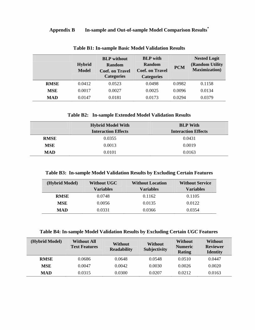
Appendix B In-sample and Out-of-sample Model Comparison Results*

Table B1: In-sample Basic Model Validation Results

Hybrid

Model

BLP without

Random

Coef. on Travel

Categories

BLP with

Random

Coef. on Travel

Categories

PCM

Nested Logit

(Random Utility

Maximization)

RMSE 0.0412 0.0523 0.0498 0.0982 0.1158

MSE 0.0017 0.0027 0.0025 0.0096 0.0134

MAD 0.0147 0.0181 0.0173 0.0294 0.0379

Table B2: In-sample Extended Model Validation Results

Hybrid Model With

Interaction Effects

BLP With

Interaction Effects

RMSE 0.0355 0.0431

MSE 0.0013 0.0019

MAD 0.0101 0.0163

Table B3: In-sample Model Validation Results by Excluding Certain Features

(Hybrid Model) Without UGC

Variables

Without Location

Variables

Without Service

Variables

RMSE 0.0748 0.1162 0.1105

MSE 0.0056 0.0135 0.0122

MAD 0.0331 0.0366 0.0354

Table B4: In-sample Model Validation Results by Excluding Certain UGC Features

(Hybrid Model) Without All

Text Features Without

Readability

Without

Subjectivity

Without

Numeric

Rating

Without

Reviewer

Identity

RMSE 0.0686 0.0648 0.0548 0.0510 0.0447

MSE 0.0047 0.0042 0.0030 0.0026 0.0020

MAD 0.0315 0.0300 0.0207 0.0212 0.0163

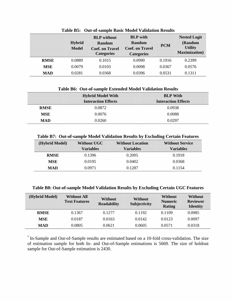
Table B5: Out-of-sample Basic Model Validation Results

Hybrid

Model

BLP without

Random

Coef. on Travel

Categories

BLP with

Random

Coef. on Travel

Categories

PCM

Nested Logit

(Random

Utility

Maximization)

RMSE 0.0889 0.1015 0.0990 0.1916 0.2399

MSE 0.0079 0.0103 0.0098 0.0367 0.0576

MAD 0.0281 0.0368 0.0396 0.0531 0.1311

Table B6: Out-of-sample Extended Model Validation Results

Hybrid Model With

Interaction Effects

BLP With

Interaction Effects

RMSE 0.0872 0.0938

MSE 0.0076 0.0088

MAD 0.0260 0.0297

Table B7: Out-of-sample Model Validation Results by Excluding Certain Features

(Hybrid Model) Without UGC

Variables

Without Location

Variables

Without Service

Variables

RMSE 0.1396 0.2005 0.1918

MSE 0.0195 0.0402 0.0368

MAD 0.0971 0.1287 0.1154

Table B8: Out-of-sample Model Validation Results by Excluding Certain UGC Features

(Hybrid Model) Without All

Text Features Without

Readability

Without

Subjectivity

Without

Numeric

Rating

Without

Reviewer

Identity

RMSE 0.1367 0.1277 0.1192 0.1109 0.0985

MSE 0.0187 0.0163 0.0142 0.0123 0.0097

MAD 0.0805 0.0621 0.0605 0.0571 0.0318

*

In-Sample and Out-of-Sample results are estimated based on a 10-fold cross-validation. The size

of estimation sample for both In- and Out-of-Sample estimations is 5669. The size of holdout

sample for Out-of-Sample estimation is 2430.

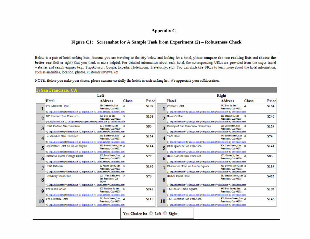
Appendix C

Figure C1: Screenshot for A Sample Task from Experiment (2) – Robustness Check

More Details on the Design of Experiment (2)

To further control for any experimental design biases and to test the robustness of our findings, we

then conducted another set of similar experiments with more stringent controls in the design and execution

of the experiment. This led to a set of 7800 user comparisons. Our additional design takes into account the

following issues:

First, to prevent each AMT worker from seeing the same ranking multiple times, we restricted each

worker to only participate in at most one ranking comparison for each city;

Second, to make sure each AMT worker is exposed to the full decision making environment as a

“real” visitor, in addition to the hotel name, address, price and class information, we provided the

URLs for each hotel’s main webpages from 5 different major (travel) search engine websites:

TripAdvisor.com, Expedia.com, Hotels.com, Travelocity.com, and Google.com. Moreover, we were

able to track whether or not a particular AMT worker clicked on any of these URLs for a particular

hotel in a particular ranking comparison task;

Third, we were able to track the exact time each AMT worker spent on a task (i.e., from the

moment an AMT worker accepted a task until the moment that worker submitted the result);

Finally, to control for the quality of the responses, we allowed only those AMT workers with a

prior approval rate higher than 95% to participate in the experiment. AMT provides an approval

rate for each worker based on the frequency with which tasks have been approved by the buyer.

This approval rate can provide information on the quality of the workers.

Our finding suggested that on average, each AMT worker spent 116.8 seconds (~ 2 minutes) per task.

Besides, more than 50% AMT workers clicked on the provided URLs to facilitate their decisions based on

the detailed information of the hotels.

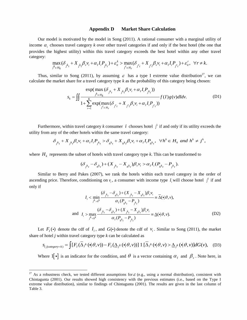
Appendix D Market Share Calculation

Our model is motivated by the model in Song (2011). A rational consumer with a marginal utility of

income i chooses travel category k over other travel categories if and only if the best hotel (the one that

provides the highest utility) within this travel category exceeds the best hotel within any other travel

category:

max( ) max( ) , .k r

k k v i I i k it r r v i I i r itj t j t j t j t j t j tk rj H j Hk r

X v I P X v I P r k

Thus, similar to Song (2011), by assuming has a type I extreme value distribution27

, we can

calculate the market share for a travel category type k as the probability of this category being chosen:

1

exp( max ( ))

( ) ( ) .

1 exp(max( ))

k k v i I i kj t j t j tkj Hkk K

r r v i I i rj t j t j trj Hrr

X v I P

s f I g v dIdv

X v I P

(D1)

Furthermore, within travel category k consumer chooses hotel if and only if its utility exceeds the

utility from any of the other hotels within the same travel category:

, ,k k k

k k v i I i k k k v i I i k kj t j t j t h t h t h tX v I P X v I P h H and h j

where kH represents the subset of hotels with travel category type k. This can be transformed to

( ) ( ) ( ).k k k k v i I i k kj t h t j t h t h t j tX X v I P P

Similar to Berry and Pakes (2007), we rank the hotels within each travel category in the order of

ascending price. Therefore, conditioning on , a consumer with income type will choose hotel if and

only if

( ) ( )min ( | , ),

( )

k k k k v ij t h t j t h t

i k kj h I k kh t j t

X X vI v

P P

and

( ) ( )max ( | , ).

( )

k k k k v ij t h t j t h t

ik kj h I k kh t j t

X X vI v

P P

(D2)

Let ( )IF denote the cdf of , and ( )G denote the cdf of . Similar to Song (2011), the market

share of hotel j within travel category type k can be calculated as

( | ) [ ( ( | , )) ( ( | , ))] 1 [ ( | , ) ( | , )] ( ),k kk kj jj jj category k I Is F v F v v v dG v

(D3)

Where 1 is an indicator for the condition, and is a vector containing and . Note here, in

27

As a robustness check, we tested different assumptions for (e.g., using a normal distribution), consistent with

Chintagunta (2001). Our results showed high consistency with the previous estimates (i.e., based on the Type I

extreme value distribution), similar to findings of Chintagunta (2001). The results are given in the last column of

Table 3.

i kj

iv iI kj

iI iv

I v

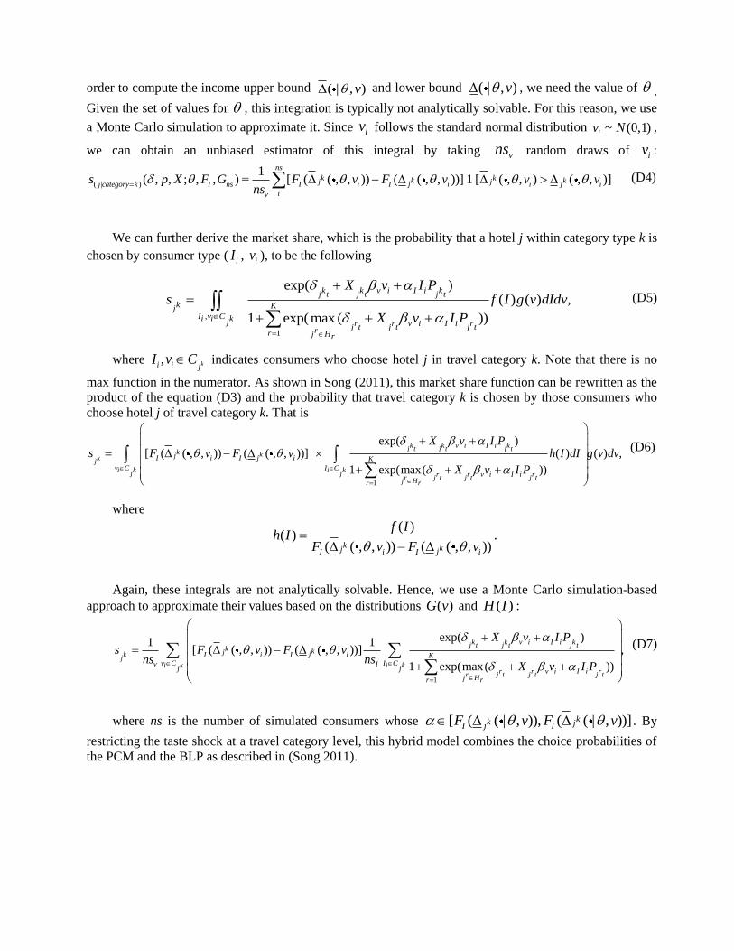
order to compute the income upper bound and lower bound , we need the value of .

Given the set of values for , this integration is typically not analytically solvable. For this reason, we use

a Monte Carlo simulation to approximate it. Since follows the standard normal distribution ,

we can obtain an unbiased estimator of this integral by taking random draws of :

( | )

1( , , ; , , ) [ ( ( , , )) ( ( , , ))] 1 [ ( , , ) ( , , )]

ns

k kk kj jj jj category k I ns I i I i i i

iv

s p X F G F v F v v vns

(D4)

We can further derive the market share, which is the probability that a hotel j within category type k is

chosen by consumer type ( iI , iv ), to be the following

,

1

exp( ) ( ) ( ) ,

1 exp(max ( ))

k k v i I i kj t j t j t

k KjI v Ci i kj r r v i I i rj t j t j trr j Hr

X v I Ps f I g v dIdv

X v I P

(D5)

where , ki i jI v C indicates consumers who choose hotel j in travel category k. Note that there is no

max function in the numerator. As shown in Song (2011), this market share function can be rewritten as the

product of the equation (D3) and the probability that travel category k is chosen by those consumers who

choose hotel j of travel category k. That is

1

exp( )[ ( ( , , )) ( ( , , ))] ( ) ( ) ,

1 exp(max( ))

k k v i I i kj t j t j tk kj jk I i I i Kj

v C I Ci k i kj j r r v i I i rj t j t j trj Hrr

X v I Ps F v F v h I dI g v dv

X v I P

(D6)

where

( )( ) .

( ( , , )) ( ( , , ))k kj jI i I i

f Ih I

F v F v

Again, these integrals are not analytically solvable. Hence, we use a Monte Carlo simulation-based

approach to approximate their values based on the distributions ( )G v and ( )H I :

1

exp( )1 1[ ( ( , , )) ( ( , , ))] ,

1 exp(max( ))

k k v i I i kj t j t j tk kj jk I i I i Kj

v C I Cv Ii k i kj j r r v i I i rj t j t j trj Hrr

X v I Ps F v F v

ns nsX v I P

(D7)

where ns is the number of simulated consumers whose [ ( ( | , )), ( ( | , ))]kk jjI IF v F v . By

restricting the taste shock at a travel category level, this hybrid model combines the choice probabilities of

the PCM and the BLP as described in (Song 2011).

( | , )v ( | , )v

iv ~ (0,1)iv N

vnsiv

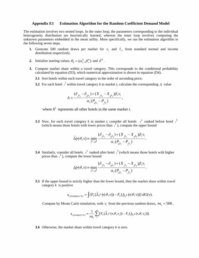
Appendix E1 Estimation Algorithm for the Random Coefficient Demand Model

The estimation involves two nested loops. In the outer loop, the parameters corresponding to the individual heterogeneity distribution are heuristically learned, whereas the inner loop involves computing the unknown parameters embedded in the mean utility. More specifically, we ran the estimation algorithm in the following seven steps.

1. Generate 500 random draws per market for iv and iI , from standard normal and income distribution respectively.

2. Initialize starting values 0 0

0 ( , )I v and 0 .

3. Compute market share within a travel category. This corresponds to the conditional probability calculated by equation (D3), which numerical approximation is shown in equation (D4).

3.1 Sort hotels within each travel category in the order of ascending price;

3.2 For each hotel k

j within travel category k in market t, calculate the corresponding value

where represents all other hotels in the same market . kh t

3.3 Now, for each travel category k in market t, consider all hotels k

h ranked before hotel k

j

(which means those hotels with lower prices than k

j ), compute the upper bound

( ) ( )( | , ) min .

( )

k k k k v ij t h t j t h t

k kj h I k kh t j t

X X vv

P P

3.4 Similarly, consider all hotels k

h ranked after hotel k

j (which means those hotels with higher prices than

kj ), compute the lower bound

( ) ( )( | , ) max .

( )

k k k k v ij t h t j t h t

k kj h I k kh t j t

X X vv

P P

3.5 If the upper bound is strictly higher than the lower bound, then the market share within travel category k is positive

( | ) [ ( ( | , )) ( ( | , ))] ( ).k kj jj category k I Is F v F v dG v

Compute by Monte Carlo simulation, with iv from the previous random draws, 500vns ,

( | )

1[ ( ( , , )) ( ( , , ))].

ns

k kj jj category k I i I i

iv

s F v F vns

3.6 Otherwise, the market share within travel category k is zero.

( ) ( ),

( )

k k k k v ij t h t j t h t

I k kh t j t

X X v

P P

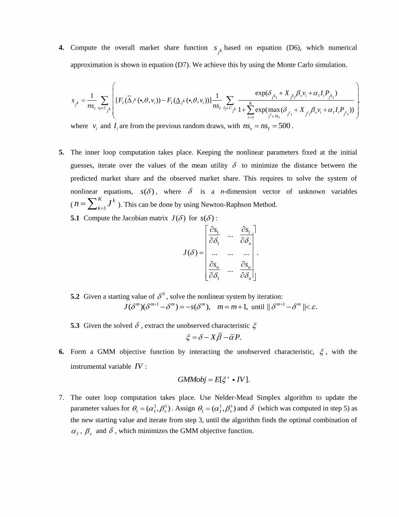
4. Compute the overall market share function kjs based on equation (D6), which numerical

approximation is shown in equation (D7). We achieve this by using the Monte Carlo simulation.

1

exp( )1 1[ ( ( , , )) ( ( , , ))] ,

1 exp(max( ))

k k v i I i kj t j t j tk kj jk I i I i Kj

v C I Cv Ii k i kj j r r v i I i rj t j t j trj Hrr

X v I Ps F v F v

ns nsX v I P

where iv and iI are from the previous random draws, with 500v Ins ns .

5. The inner loop computation takes place. Keeping the nonlinear parameters fixed at the initial

guesses, iterate over the values of the mean utility to minimize the distance between the

predicted market share and the observed market share. This requires to solve the system of

nonlinear equations, ( )s , where is a n-dimension

vector of unknown variables

(1

K k

kn J

). This can be done by using Newton-Raphson Method.

5.1 Compute the Jacobian matrix ( )J for ( )s :

1 1

1

1

...

( ) ... ... ... .

...

n

n n

n

s s

J

s s

5.2 Given a starting value of 0 , solve the nonlinear system by iteration:

1( )( ) ( ), 1,m m m mJ s m m until 1|| || .m m

5.3 Given the solved , extract the unobserved characteristic

.X P

6. Form a GMM objective function by interacting the unobserved characteristic, , with the

instrumental variable IV :

[ ' ].GMMobj E IV

7. The outer loop computation takes place. Use Nelder-Mead Simplex algorithm to update the

parameter values for 1 1

1 ( , )I v . Assign 1 1

1 ( , )I v and (which was computed in step 5) as

the new starting value and iterate from step 3, until the algorithm finds the optimal combination of

I , v and , which minimizes the GMM objective function.

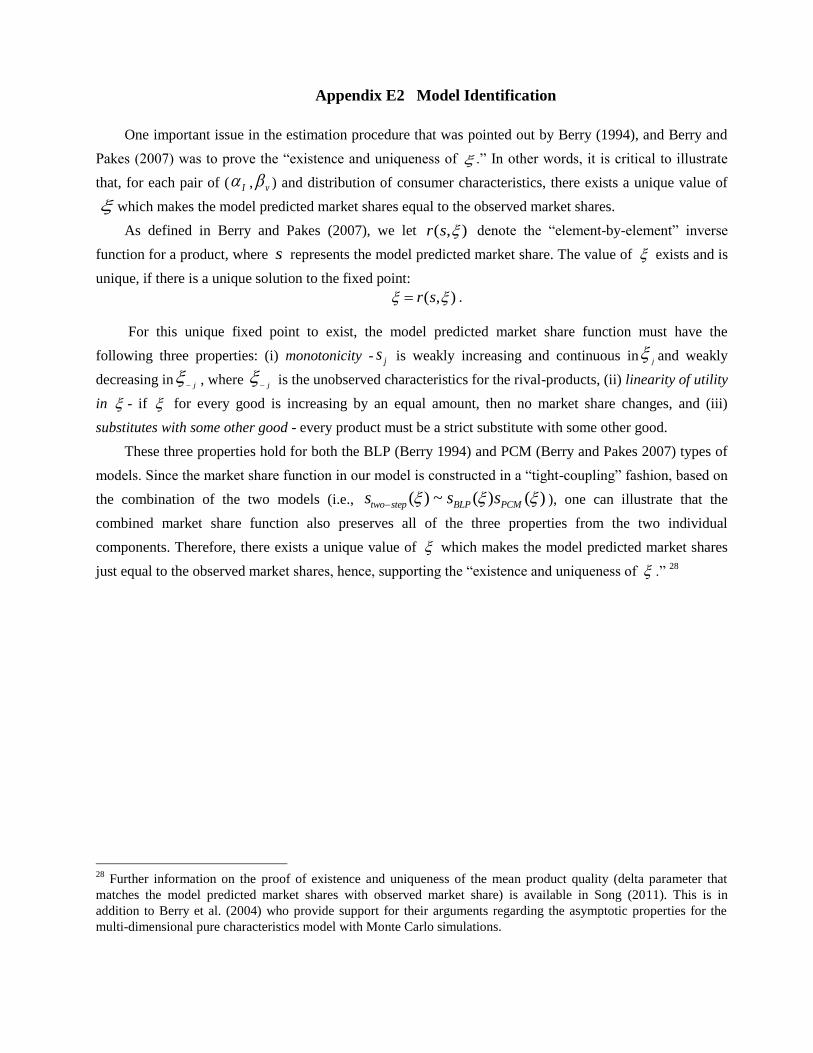
Appendix E2 Model Identification

One important issue in the estimation procedure that was pointed out by Berry (1994), and Berry and

Pakes (2007) was to prove the “existence and uniqueness of .” In other words, it is critical to illustrate

that, for each pair of ( I , v ) and distribution of consumer characteristics, there exists a unique value of

which makes the model predicted market shares equal to the observed market shares.

As defined in Berry and Pakes (2007), we let ( , )r s denote the “element-by-element” inverse

function for a product, where s represents the model predicted market share. The value of exists and is

unique, if there is a unique solution to the fixed point:

( , )r s .

For this unique fixed point to exist, the model predicted market share function must have the

following three properties: (i) monotonicity - js is weakly increasing and continuous in j and weakly

decreasing in j

, where j

is the unobserved characteristics for the rival-products, (ii) linearity of utility

in - if for every good is increasing by an equal amount, then no market share changes, and (iii)

substitutes with some other good - every product must be a strict substitute with some other good.

These three properties hold for both the BLP (Berry 1994) and PCM (Berry and Pakes 2007) types of

models. Since the market share function in our model is constructed in a “tight-coupling” fashion, based on

the combination of the two models (i.e., ( ) ~ ( ) ( )two step BLP PCMs s s ), one can illustrate that the

combined market share function also preserves all of the three properties from the two individual

components. Therefore, there exists a unique value of which makes the model predicted market shares

just equal to the observed market shares, hence, supporting the “existence and uniqueness of .” 28

28

Further information on the proof of existence and uniqueness of the mean product quality (delta parameter that

matches the model predicted market shares with observed market share) is available in Song (2011). This is in

addition to Berry et al. (2004) who provide support for their arguments regarding the asymptotic properties for the

multi-dimensional pure characteristics model with Monte Carlo simulations.

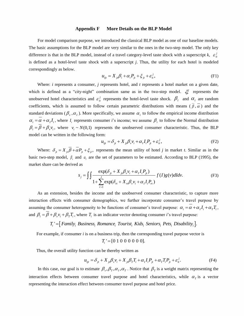
Appendix F More Details on the BLP Model

For model comparison purpose, we introduced the classical BLP model as one of our baseline models.

The basic assumptions for the BLP model are very similar to the ones in the two-step model. The only key

difference is that in the BLP model, instead of a travel category-level taste shock with a superscript k, j

it

is defined as a hotel-level taste shock with a superscript j. Thus, the utility for each hotel is modeled

correspondingly as below.

,j

ijt jt i i jt jt itu X P (F1)

Where: i represents a consumer, j represents hotel, and t represents a hotel market on a given date,

which is defined as a “city-night” combination same as in the two-step model. represents the

unobserved hotel characteristics and j

it represents the hotel-level taste shock. and are random

coefficients, which is assumed to follow certain parametric distributions with means ( , ) and the

standard deviations ( v , I ). More specifically, we assume i to follow the empirical income distribution

i I iI , where represents consumer i’s income; we assume i to follow the Normal distribution

i v iv , where represents the unobserved consumer characteristic. Thus, the BLP

model can be written in the following form:

,j

ijt jt jt v i I i jt itu X v I P

(F2)

Where: ,jt jt jt jtX P represents the mean utility of hotel j in market t. Similar as in the

basic two-step model, and are the set of parameters to be estimated. According to BLP (1995), the

market share can be derived as

1

exp( )( ) ( ) .

1 exp( )

jt jt v i I i jt

j J

rt rt v i I i rt

r

X v I Ps f I g v dIdv

X v I P

(F3)

As an extension, besides the income and the unobserved consumer characteristic, to capture more

interaction effects with consumer demographics, we further incorporate consumer’s travel purpose by

assuming the consumer heterogeneity to be functions of consumer’s travel purpose: i I i T iI T ,

and i v i T iv T , where iT is an indicator vector denoting consumer i’s travel purpose:

' .i i i i i i i i iT Family Business Romance Tourist Kids Seniors Pets Disability

For example, if consumer i is on a business trip, then the corresponding travel purpose vector is

' [0 1 0 0 0 0 0 0].iT

Thus, the overall utility function can be thereby written as

.j

ijt jt jt v i jt T i I i jt T i jt itu X v X T I P T P (F4)

In this case, our goal is to estimate , , ,v T I T . Notice that T is a weight matrix representing the

interaction effects between consumer travel purpose and hotel characteristics, while T is a vector

representing the interaction effect between consumer travel purpose and hotel price.

i i

iI

~ (0,1)iv N

v I

Appendix G More Details on UGC Mining

(G-1) Extraction of Location Characteristics using Social Geotagging and Image Classification

As mentioned in Subsection 3.3, to allow for the automated tagging of areas that lack tags from the

human tagging process, we use automatic image classification techniques of satellite images to tag location

features that can influence hotel demand. Consider, for example, the case where we are trying to

automatically identify whether a hotel is located “Near a beach,” or “Near downtown.” Towards this, we

extracted hybrid satellite images (sized 256 × 256 pixels) using the Visual Earth Tile System 29

, for each of

the (thousands) of hotel venues located in the US, with four different zoom levels for each. These 4 x 1497

images were used to extract information about the surroundings of the hotel, through image classification

and human inspection using AMT. For better understanding, below are two examples of the images used in

our analysis.

Beach Downtown

To automatically tag satellite images, we first needed to train our classification model. To build a

“training set,” we used information from two sources: (i) locations tagged by users on a social tagging site

such as Geonames.org or (ii) locations annotated by users on AMT. We built the image classifiers as

follows: First, we randomly selected a set of 121 hotels and requested five AMT users to label each

example according to its corresponding satellite images from four different zoom levels. The labelers

answered whether there is a beach in the image, or whether the image is that of a downtown area. We

applied a simple majority voting method to make the final decision from the multi-labels of the example.

Second, we trained a Support Vector Machines (SVM) classifier on this dataset and used the trained SVM

classifier to classify the images that corresponded to the remaining hotels. Prior work has shown that non-

parametric classifiers, such as Neural Networks, Decision Trees, and Support Vector Machines (SVM)

provide better results than parametric classifiers in complex landscapes (Lu and Weng 2007). Therefore,

we tested various non-parametric classification techniques. These include (i) Decision Trees, which are

widely used for training and classification of remotely sensed image data (due to their ability to generate

human interpretable decision rules and its speed in training and classification), and (ii) Support Vector

29

http://msdn2.microsoft.com/en-us/library/bb259689.aspx

Machines (SVM), that are highly accurate and perform well for a wide variety of classification tasks

(Fukuda and Hirosawa 2001).

We conducted a small study to examine the performance of the classifier out-of-sample data. We

classified the out of sample images using AMT; our results illustrated that our SVM classifier had an

accuracy of 91.2% for the “beach” image classification and 80.7% for the “downtown” image

classification. We also used the C4.5 algorithm for the classification, and noticed an accuracy increase for

“Near a beach” and a decrease for “Near downtown.” The main reason for this is that “beach" images often

contain a “sand strip," together with an “ocean margin" well distributed in density. This typically provides

more stable and distinct textural information for the “beach" images, thus making them easier to

distinguish.

Moreover, as a robustness check, we extracted the two location characteristics “Near a beach” and

“Near downtown” using geo-tagging approach via the site Geonames.org. In particular, the geo-tagging

process and the image classification process were conducted independently. We found that the overlapping

rate between the two sets of results (i.e., acquired independently from the geo-tagging approach and from

the image classification approach) is very high: For “Near a beach,” this overlapping rate is 92.3%, and for

“Near the downtown,” this overlapping rate is 85.1%. This additional test provides us with high confidence

on our image tagging results.

(G-2) Extraction of Textual Quality of Customer Reviews

In regards to the extraction of textual quality of customer reviews, as discussed in Subsection 3.5, we

looked into two text style features “subjectivity” and “readability” as the evaluating criteria. To capture the

review textual style comprehensively, we used a multiple-item method for subjectivity and readability. We

included two sub-features for subjectivity and five sub-features for readability, each of which measures the

review text style.

We observed that there are two types of reviews, from the stylistic point of view. There are reviews

that list “objective" information, listing the characteristics of the hotel, and giving an alternate description

that confirms (or rejects) the description given by the hotel. The other types of reviews are those with

“subjective," sentimental information, in which the reviewers give a very personal description of the hotel,

and give information that, typically, does not appear in the official description of the hotel.

We distinguished the extent of “subjective assessments” in the reviews by deriving a review-level

numerical score for the degree of subjectivity. More specifically, we used the methods from Ghose and

Ipeirotis (2011) who build on the methods in Pang and Lee (2004). In particular, objective information is

considered the information that also appears in the hotel-provided description, and subjective is everything

else. To infer the probability of review subjectivity, we trained a classifier by using as “objective”

documents the hotel-generated descriptions from the websites of Travelocity and TripAdvisor. We then

randomly retrieved 1000 reviews to construct the “subjective” examples of the training set.30

After

constructing the classifiers, we used the resulting classification models in the remaining, unseen reviews.

Instead of classifying each review as subjective or objective, we instead classified each sentence in each

review as either “objective" or “subjective," keeping the probability of being subjective for each sentence.

By doing so, we were able to acquire a subjectivity confidence score for each sentence in a review, hence

deriving the mean and standard deviation of this score as the subjectivity measurements for that review.

These numerical scores are able to distinguish how likely a review contains subjective assessments as

opposed to objective descriptions.

We also look into the impact of “Readability,” which is a proxy for the difficulty faced by people

when reading online reviews. Past research has shown that easy-reading text improves comprehension,

retention, and reading speed, and that the average reading level of the US adult population is at the eighth

grade level (White 2003). Specifically, for each hotel, we collected all existing reviews to examine the

average number of characters per review, average number of syllables per review, average number of

spelling errors per review, and the average length of the sentence as a “Complexity” measurement (total

number of characters divided by the total number of sentences). To avoid idiosyncratic errors peculiar to a

specific readability metric, we computed a set of metrics for each review. Specifically, we computed the

30

We conducted the training process by using a 4-gram Dynamic Language Model classifier provided by the lingpipe

toolkit. “Lingpipe” is a tool kit provided online for processing text using computational linguistics (More information

can be found at http://alias-i.com/lingpipe/).

following: Automated Readability Index, Coleman-Liau Index, Flesch Reading Ease, Flesch-Kincaid Grade

Level, Gunning and SMOG. For brevity, we only show results with SMOG Index in the paper although all

the other readability measures yield similar results.

Furthermore, previous studies have shown that the social identity information of reviewers in an

online community shapes community members' judgment of the products. In other words, the prevalence of

reviewer disclosure of identity information is associated with changes in product sales (Forman et al. 2008).

Therefore, consistent with prior work, we include the characteristic that captures the level of reviewers’

disclosure of their identity information – “real name or location.” More specifically, this binary

characteristic describes whether or not a reviewer had revealed her real name or location information on the

reviewer profile page of Travelocity and TripAdvisor.

In sum, our analysis identifies 5 broad types of characteristics in this category: (i) total number of

reviews, (ii) overall review rating, (iii) review subjectivity (mean and variance), (iv) review readability (the

number of characters, syllables, and spelling errors, complexity and SMOG Index), and (v) the disclosure

identity information by the reviewer.

(G-3) Text Feature Extraction and Sentimental Analysis

Towards extracting the additional text features discussed in Subsection 4.3, we build on the work of

Hu and Liu (2004), Popescu and Etzioni (2005), Archak et al. (2011). More specifically, we conduct the

text mining process in the following three steps:

(1) Text Feature Extraction.

First, we extracted all the evaluation phrases (adjectives and adverbs) that are being used to evaluate

the individual service features (for example, for the feature “hotel staff” we extracted phrases like

“helpful,” “smiling,” “rude,” “responsive,” etc) . The process of extracting user evaluation phrases can, in

general, be automated. Following the automated approach introduced previously (e.g., Archak et al. 2011),

we use a POS (part-of-speech) tagger to identify frequently mentioned nouns and noun phrases, which we

consider candidate hotel features. We then cluster these phrases, using WordNet (Fellbaum 1998) and then

use a context-sensitive hierarchical agglomerative clustering algorithm (Manning and Schutze 1999) to

cluster further the identified nouns and noun phrases into clusters of similar nouns and noun phrases. The

resulting set of clusters corresponds to the set of identified product features mentioned in the reviews. For

our analysis, we kept the top-5 most frequently mentioned features, which were hotel staff, food quality,

bathroom, parking facilities, and bedroom quality.31

Besides, as suggested in Archak et al. (2011), in

addition to the fully automated tool we can also use a semi-automated crowdsourcing approach via Amazon

Mechanical Turk, by asking AMT workers to manually process each review and extract evaluation phrases

for any given product feature.

(2) Sentimental Analysis.

For sentimental analysis, we extract all the evaluation phrases (adjectives and adverbs) that are being

used to evaluate the individual service features (for example, for the feature “hotel staff” we extract

phrases like “helpful,” “smiling,” “rude,” “responsive,” etc) . To measure the meaning of these evaluation

phrases, we used Amazon Mechanical Turk to exogenously assign explicit polarity semantics to each word.

To compute the scores, we used AMT to create our ontology, with the scores for each evaluation phrase.

Our process for creating these “external” scores was done using the methodology of Archak et al. (2011).

We asked nine AMT workers to look at the pair of the evaluation phrase together with the product feature,

31

To select the top 5 features, we first processed all the reviews for each hotel, and extracted text features (i.e., terms)

that appeared frequently in the reviews for each hotel. For example, for Hotel A the features extracted based on the

reviews for Hotel A can be “bed”, “bathroom” and “pool”; for Hotel B the features can be “bed”, “bathroom” and

“restaurant”. Then, we selected the top 5 most frequently extracted features across all hotels. In our example, the

features will be “bed” and “bathroom”. The top 5 features that we selected in our study covered 80% of the hotels,

which means that for 80% of the hotels the extracted text features contain these 5 features. While technically possible,

we did not consider more textual features because the frequency in which the additional features are mentions drops

significantly, and therefore we would not be able to have a robust measurement for these textually-inferred features

for a very significant fraction of the hotels in our dataset.

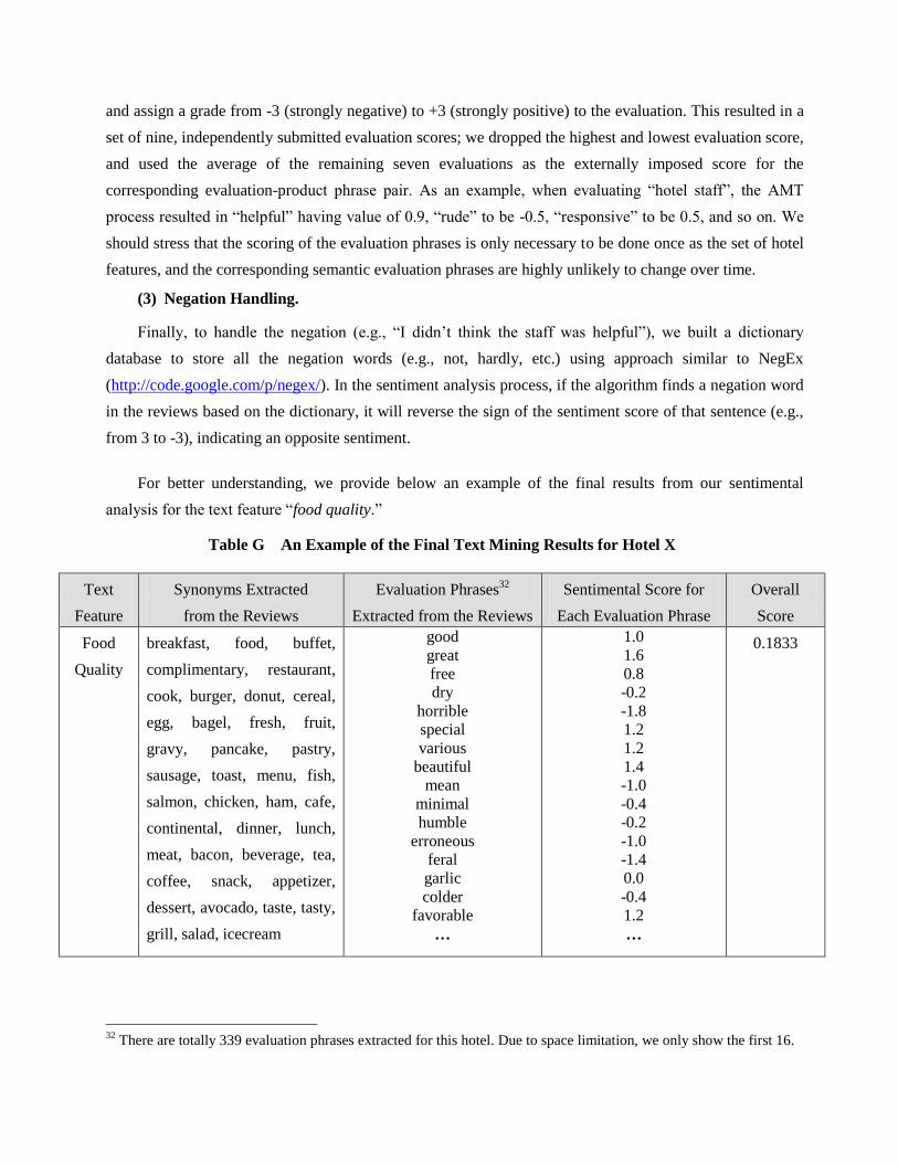
and assign a grade from -3 (strongly negative) to +3 (strongly positive) to the evaluation. This resulted in a

set of nine, independently submitted evaluation scores; we dropped the highest and lowest evaluation score,

and used the average of the remaining seven evaluations as the externally imposed score for the

corresponding evaluation-product phrase pair. As an example, when evaluating “hotel staff”, the AMT

process resulted in “helpful” having value of 0.9, “rude” to be -0.5, “responsive” to be 0.5, and so on. We

should stress that the scoring of the evaluation phrases is only necessary to be done once as the set of hotel

features, and the corresponding semantic evaluation phrases are highly unlikely to change over time.

(3) Negation Handling.

Finally, to handle the negation (e.g., “I didn’t think the staff was helpful”), we built a dictionary

database to store all the negation words (e.g., not, hardly, etc.) using approach similar to NegEx

(http://code.google.com/p/negex/). In the sentiment analysis process, if the algorithm finds a negation word

in the reviews based on the dictionary, it will reverse the sign of the sentiment score of that sentence (e.g.,

from 3 to -3), indicating an opposite sentiment.

For better understanding, we provide below an example of the final results from our sentimental

analysis for the text feature “food quality.”

Table G An Example of the Final Text Mining Results for Hotel X

Text

Feature

Synonyms Extracted

from the Reviews

Evaluation Phrases32

Extracted from the Reviews

Sentimental Score for

Each Evaluation Phrase

Overall

Score

Food

Quality

breakfast, food, buffet,

complimentary, restaurant,

cook, burger, donut, cereal,

egg, bagel, fresh, fruit,

gravy, pancake, pastry,

sausage, toast, menu, fish,

salmon, chicken, ham, cafe,

continental, dinner, lunch,

meat, bacon, beverage, tea,

coffee, snack, appetizer,

dessert, avocado, taste, tasty,

grill, salad, icecream

good

great

free

dry

horrible

special

various

beautiful

mean

minimal

humble

erroneous

feral

garlic

colder

favorable

…

1.0

1.6

0.8

-0.2

-1.8

1.2

1.2

1.4

-1.0

-0.4

-0.2

-1.0

-1.4

0.0

-0.4

1.2

…

0.1833

32

There are totally 339 evaluation phrases extracted for this hotel. Due to space limitation, we only show the first 16.

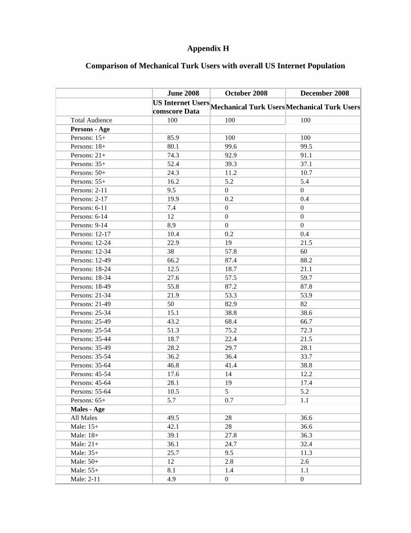
Appendix H

Comparison of Mechanical Turk Users with overall US Internet Population

June 2008 October 2008 December 2008

US Internet Users

comscore Data Mechanical Turk Users Mechanical Turk Users

Total Audience 100 100 100

Persons - Age

Persons: 15+ 85.9 100 100

Persons: 18+ 80.1 99.6 99.5

Persons: 21+ 74.3 92.9 91.1

Persons: 35+ 52.4 39.3 37.1

Persons: 50+ 24.3 11.2 10.7

Persons: 55+ 16.2 5.2 5.4

Persons: 2-11 9.5 0 0

Persons: 2-17 19.9 0.2 0.4

Persons: 6-11 7.4 0 0

Persons: 6-14 12 0 0

Persons: 9-14 8.9 0 0

Persons: 12-17 10.4 0.2 0.4

Persons: 12-24 22.9 19 21.5

Persons: 12-34 38 57.8 60

Persons: 12-49 66.2 87.4 88.2

Persons: 18-24 12.5 18.7 21.1

Persons: 18-34 27.6 57.5 59.7

Persons: 18-49 55.8 87.2 87.8

Persons: 21-34 21.9 53.3 53.9

Persons: 21-49 50 82.9 82

Persons: 25-34 15.1 38.8 38.6

Persons: 25-49 43.2 68.4 66.7

Persons: 25-54 51.3 75.2 72.3

Persons: 35-44 18.7 22.4 21.5

Persons: 35-49 28.2 29.7 28.1

Persons: 35-54 36.2 36.4 33.7

Persons: 35-64 46.8 41.4 38.8

Persons: 45-54 17.6 14 12.2

Persons: 45-64 28.1 19 17.4

Persons: 55-64 10.5 5 5.2

Persons: 65+ 5.7 0.7 1.1

Males - Age

All Males 49.5 28 36.6

Male: 15+ 42.1 28 36.6

Male: 18+ 39.1 27.8 36.3

Male: 21+ 36.1 24.7 32.4

Male: 35+ 25.7 9.5 11.3

Male: 50+ 12 2.8 2.6

Male: 55+ 8.1 1.4 1.1

Male: 2-11 4.9 0 0

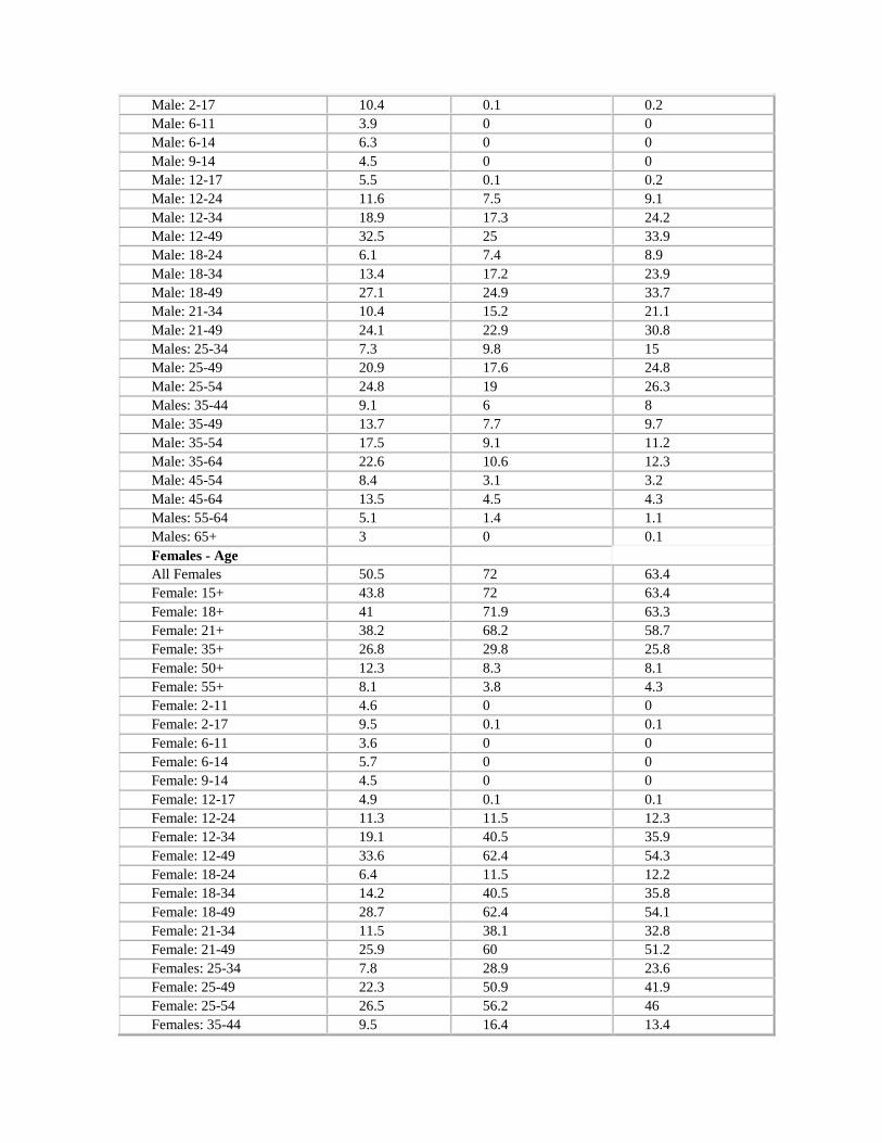
Male: 2-17 10.4 0.1 0.2

Male: 6-11 3.9 0 0

Male: 6-14 6.3 0 0

Male: 9-14 4.5 0 0

Male: 12-17 5.5 0.1 0.2

Male: 12-24 11.6 7.5 9.1

Male: 12-34 18.9 17.3 24.2

Male: 12-49 32.5 25 33.9

Male: 18-24 6.1 7.4 8.9

Male: 18-34 13.4 17.2 23.9

Male: 18-49 27.1 24.9 33.7

Male: 21-34 10.4 15.2 21.1

Male: 21-49 24.1 22.9 30.8

Males: 25-34 7.3 9.8 15

Male: 25-49 20.9 17.6 24.8

Male: 25-54 24.8 19 26.3

Males: 35-44 9.1 6 8

Male: 35-49 13.7 7.7 9.7

Male: 35-54 17.5 9.1 11.2

Male: 35-64 22.6 10.6 12.3

Male: 45-54 8.4 3.1 3.2

Male: 45-64 13.5 4.5 4.3

Males: 55-64 5.1 1.4 1.1

Males: 65+ 3 0 0.1

Females - Age

All Females 50.5 72 63.4

Female: 15+ 43.8 72 63.4

Female: 18+ 41 71.9 63.3

Female: 21+ 38.2 68.2 58.7

Female: 35+ 26.8 29.8 25.8

Female: 50+ 12.3 8.3 8.1

Female: 55+ 8.1 3.8 4.3

Female: 2-11 4.6 0 0

Female: 2-17 9.5 0.1 0.1

Female: 6-11 3.6 0 0

Female: 6-14 5.7 0 0

Female: 9-14 4.5 0 0

Female: 12-17 4.9 0.1 0.1

Female: 12-24 11.3 11.5 12.3

Female: 12-34 19.1 40.5 35.9

Female: 12-49 33.6 62.4 54.3

Female: 18-24 6.4 11.5 12.2

Female: 18-34 14.2 40.5 35.8

Female: 18-49 28.7 62.4 54.1

Female: 21-34 11.5 38.1 32.8

Female: 21-49 25.9 60 51.2

Females: 25-34 7.8 28.9 23.6

Female: 25-49 22.3 50.9 41.9

Female: 25-54 26.5 56.2 46

Females: 35-44 9.5 16.4 13.4

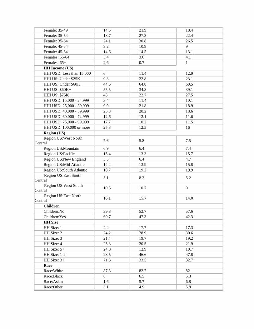
Female: 35-49 14.5 21.9 18.4

Female: 35-54 18.7 27.3 22.4

Female: 35-64 24.1 30.8 26.5

Female: 45-54 9.2 10.9 9

Female: 45-64 14.6 14.5 13.1

Females: 55-64 5.4 3.6 4.1

Females: 65+ 2.6 0.7 1

HH Income (US)

HHI USD: Less than 15,000 6 11.4 12.9

HHI US: Under $25K 9.3 22.8 23.1

HHI US: Under $60K 44.5 64.8 60.5

HHI US: $60K+ 55.5 34.8 39.1

HHI US: $75K+ 43 22.7 27.5

HHI USD: 15,000 - 24,999 3.4 11.4 10.1

HHI USD: 25,000 - 39,999 9.9 21.8 18.9

HHI USD: 40,000 - 59,999 25.3 20.2 18.6

HHI USD: 60,000 - 74,999 12.6 12.1 11.6

HHI USD: 75,000 - 99,999 17.7 10.2 11.5

HHI USD: 100,000 or more 25.3 12.5 16

Region (US)

Region US:West North

Central 7.6 5.8 7.5

Region US:Mountain 6.9 6.4 7.4

Region US:Pacific 15.4 13.3 15.7

Region US:New England 5.5 6.4 4.7

Region US:Mid Atlantic 14.2 13.9 15.8

Region US:South Atlantic 18.7 19.2 19.9

Region US:East South

Central 5.1 8.3 5.2

Region US:West South

Central 10.5 10.7 9

Region US:East North

Central 16.1 15.7 14.8

Children

Children:No 39.3 52.7 57.6

Children:Yes 60.7 47.3 42.3

HH Size

HH Size: 1 4.4 17.7 17.3

HH Size: 2 24.2 28.9 30.6

HH Size: 3 21.4 19.7 19.2

HH Size: 4 25.3 20.5 21.9

HH Size: 5+ 24.8 12.9 10.7

HH Size: 1-2 28.5 46.6 47.8

HH Size: 3+ 71.5 33.5 32.7

Race

Race:White 87.3 82.7 82

Race:Black 8 6.5 5.3

Race:Asian 1.6 5.7 6.8

Race:Other 3.1 4.9 5.8