Detecting and Monitoring Vegetation Water Stress Using

Remote Sensing Tools in Saratov Region, Russia.

MSc Thesis by Wisse Beets

23 November 2009

Detecting and Monitoring Vegetation Water Stress Using

Remote Sensing Tools in Saratov Region, Russia.

Master thesis Land Degradation and Development Group submitted in partial fulfillment of the

degree of Master of Science in International Land and Water Management at Wageningen

University, the Netherlands.

Study carried for the DESIRE project ŧ.

Study program:

MSc International Land and Water Management (MIL)

Student registration number:

840114044120

LDD 80336

Supervisor(s):

Dr. Eli Argaman

Dr. Simone Verzandvoort

Dr. Koos Groen

Examinator:

Prof.dr.ir. L. Stroosnijder

Date: 23 November 2009

Wageningen University, Land Degradation and Development Group

Moscow State University of Environmental Engineering

Vrije Universiteit Amsterdam, Faculty of Earth and Life Sciences

‡ Desertification Mitigation and Remediation of Land - a Global Approach for Local Solutions), funded by European Commission, Directorate

General for Research under Framework Programme 6, Global Change and Ecosystems (Contract Number 037046 GOCE)

Abstract

This study is carried out within the DESIRE project, an EU project that aims to reduce

land degradation and desertification in fragile agricultural areas. This specific study

aimed to develop a new simple methodology to detect crop water stress in a dryland

area in Southwest Russia. In this area irrigation is necessary to be able to grow crops,

but over-application of irrigation water can cause solution of salts in the subsoil.

Subsequently, a rising groundwater table due to irrigation can lead to transportation of

these salts to the active root zone, causing crop stress and ultimately crop starvation. If

crop waters stress is known, the ideal amount of water application can be determined.

Current ways of measuring crop water stress are too expensive and complicated to

carry out in this area, so the need for a simple methodology is urgent. Known crop

water stress measurements were carried out on two Alfalfa fields, using thermal

infrared and plant physiological measurements. These results are compared with a

newly developed methodology making use of visible light remote sensing strategies. It

appears that the newly developed methodology might provide a valid and easy way to

determine crop water stress on point and field scale, with the possibility to spatially

expand this strategy using airplane and satellite images.

1. Introduction

Degradation of arable land and accompanying low crop yields form a serious threat to

agricultural productivity, welfare and global food supplies in various arid to semi-arid

areas around the world (EEA 2003). The use of inefficient irrigation systems for long

timescales in dryland areas is a major cause of land degradation and desertification

(O’Hara et al, 1997), which means the loss of biological and economic productivity of

land in dryland areas (UNEP 1994). This is also the case in Southwest Russia, where

areas are affected by unwanted side effects of irrigation (DESIRE project website). These

side effects can cause severe crop water stress, and include increasing soil salinity, out

washing of nutrients and decreasing soil fertility.

Intense irrigation in the Saratov region in southwest Russia has initially increased crop

yield in the 1960s. Irrigation water was and still is extracted via irrigation channels

from the Volga River, and from water harvesting practices to compensate for the low

soil available water during the short growing season (Gabchenko, 2008). Too much

(inefficient) irrigation however, has had the side effect of flushing away valuable

nutrients from the soil and raising the groundwater table. The groundwater quality in

both areas is affected by dissolution of salts from the sediments deposited during the

transgression of the Caspian Sea during the Khvalynian transgression, in 16-10 ka BP

(Svitoch, 2008). During this transgression, a thick layer of marine loams was deposited,

containing high salt concentrations (Gabchenko, 2008). These salts are transported to

the active root zone, because of inadequate land management, like excessive irrigation

and plowing. These anthropogenic processes increasing salt concentrations in the

agricultural interface are referred to as secondary salinization. A form of salinization,

referred to as alkalinization, is believed to be an important factor for decreasing crop

yield in this area. Alkalinization is the process where mainly sodium carbonates are

transported by groundwater to the active root zone, and partly precipitates in the

subsoil (Condom et al, 1999). These soils are characterized by a high pH, a relative low

EC, and a high concentration of sodium ions. Also, precipitated salts and cracks in the

topsoil can be observed (Metternicht, 2001).

Detecting and monitoring crop water stress is important, because it tells us about the

impact of degradation processes on the crops throughout the growing season. One way

to get an indicator for crop water stress is measuring plant water content; fresh

biomass minus dry biomass. This is a very time consuming and destructive method, so

it’s not easily applicable to construct time series of crop water stress. A more used

methodology is developed by Idso et al, 1981 and Jackson et al, 1981 using remote

sensing technology in the thermal infrared (TIR) spectrum. The TIR emittance of a

crop’s canopy combined with air temperature and measurements of the vapor pressure

deficit can be used to determine the evaporative state of the crop, and to calculate a

crop water stress index (CWSI). This method requires several measurements, and a

certain amount of equipment that is not available to most farmers in the region.

Therefore the aim of this study is to develop a new methodology to detect and monitor

this CWSI using the most simple and available tools. This methodology will be based on

the remote sensing of visible light (VIS) reflectance. If the new methodology appears to

be applicable to detect water stress, VIS satellite images can be used to easily map and

monitor crop water stress from space.

Plant physiological parameters (plant height, yield, LAI, etc.) have proven to be

indicators for crop water stress during the growing season (Hatfield et al, 1993 and

Lannucci et al, 2002). This stress results in a lower amount of chlorophyll in the

biomass. Also, vegetation suffering a severe water deficit will stop evaporating, and

wilk. Chlorophyll concentration, shadows caused by wilking vegetation and the amount

of bare soil are parameters that influence the VIS reflectance, measured using a digital

camera. To test if VIS reflectance can provide a methodology for measuring the CWSI in

this study, TIR and VIS reflectance, along with plant physiology and meteorological

parameters will be measured and analyzed to compare the new methodology with the

previously developed methodologies. Also soil properties like soil moisture, pH and EC

will be measured to detect the influence of salinization, alkalinization and soil water

content on the crop water stress.

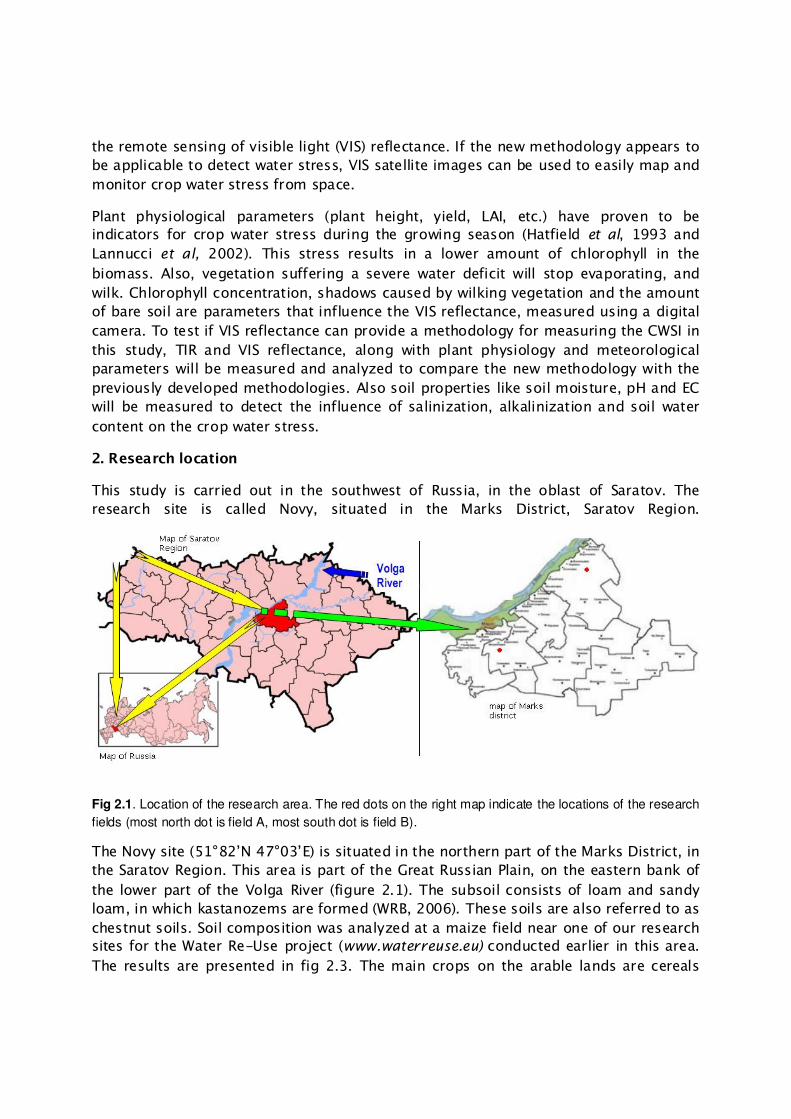
2. Research location

This study is carried out in the southwest of Russia, in the oblast of Saratov. The

research site is called Novy, situated in the Marks District, Saratov Region.

Fig 2.1. Location of the research area. The red dots on the right map indicate the locations of the research

fields (most north dot is field A, most south dot is field B).

The Novy site (51°82’N 47°03’E) is situated in the northern part of the Marks District, in

the Saratov Region. This area is part of the Great Russian Plain, on the eastern bank of

the lower part of the Volga River (figure 2.1). The subsoil consists of loam and sandy

loam, in which kastanozems are formed (WRB, 2006). These soils are also referred to as

chestnut soils. Soil composition was analyzed at a maize field near one of our research

sites for the Water Re-Use project (www.waterreuse.eu) conducted earlier in this area.

The results are presented in fig 2.3. The main crops on the arable lands are cereals

(50%) and forage crops (20%). Also, a vast amount of cattle grazes in the area, mainly

consisting of pigs, sheep and cows. This study will focus on an important forage crop;

Alfalfa.

Fig 2.2 Land use map Fig 2.3 Soil composition

The location is classified as an area with highly degraded soils (FAO report, 2008 ). The

dry steppe land climate has a long summer; from May to September, with temperatures

reaching up to 45ºC degrees. The winter lasts from December to March, when up to

28,5 cm of snowfall can take place and minimum temperatures reach to 80º colder

than in summer, to minus 35ºC. Total yearly precipitation averages at 400 mm/year,

and a major part of this precipitates as snow during the winter. Since precipitation in

summer is low, and potential evaporation is high, natural water availability for crops is

low. All the meteorological data measured during the fieldwork is presented in figure

2.4. Therefore, cultivation without irrigation is very risky and around almost all of the

cultivated area is being irrigated. However, this percentage is decreasing since the

irrigation systems are over 40 years old, and need replacement, and due to limited

availability of financial needs this is not always possible. Therefore currently only

around 75% of the cultivated area is being irrigated.

Soil Composition

sand

silt

clay

Fig 2.4. All weather data measured during the fieldwork in July. The numbers on the x-axis are the days of

July. All blue lines are mean daily (24h) values, with the red line as 5-day moving average, to show the

general trend. For precipitation and potential evaporation the values are not mean but summed daily

values.

Although irrigation is needed to supply enough water for the crops, excessive irrigation

can lead to problems. A major cause for land degradation in the Novy site is the long

timescale of excessive water application for agriculture (DESIRE project site description

of Novy). In 1960 large scale irrigation systems were constructed, pumping water from

the Volga into channels. The water from these channels is mainly used for pivot

(sprinkler) irrigation. An example of a pivot system and an irrigation channel are

presented in figure 2.5.

0

10

20

1 3 5 7 9 11 13 15 17 1921 23 25 27 2931

mm

/d

ay

Precipitation

0

100

200

300

400

500

01 03 05 07 0911 13 15 17 19 21 23 25 27 29 31

MW

/m

2

Radiation

0

20

40

01 0305 07 0911 1315 17 1921 2325 27 2931

Ce

lsiu

s D

eg

ree

s

Air Temperature

0

2

4

01 03 05 07 09 11 13 15 17 19 21 23 25 27 29 31m

/s

Wind Speed

0

20

40

60

80

100

01 0305070911131517 19212325272931

%

Relative Humidity

0

20

40

01 03 05 07 09 11 13 15 17 19 21 23 25 27 29 31

mm

/d

ay

Potential Evaporation

Fig 2.5. Pivot system at work (left) and an irrigation channel (right), which supplies the water to the pivots.

During 40 years of intensive irrigation the groundwater table has raised significantly,

from a minimal depth of 5-7 meters prior to the irrigation systems, to the active root

zone at present (Pankova, 1993). This groundwater table raise has a big impact on the

minerals in the soil and the soil texture, mainly due to two effects; (1) salts from

previously unsaturated sediments are transported upwards creating alkanized or

salinized environments in the plant root zone and (2) washing of soil layers diminishes

the soil organic matter, increasing soil compaction and worsening soil physical

parameters like hydraulic conductivity and retention capacity.

Apart from the pivot systems, there are two other types of irrigation applied in this

region. Furrow (channel) irrigation is used for smaller scale irrigation of vegetables,

close to the water supply channels. This system is more suitable for vegetable farming

then pivot irrigation, but causes water erosion and an outflow of valuable nutrients in

the region. Another irrigation system, drip irrigation, is in an experimental phase in this

area. Within the DESIRE project drip irrigation is installed at several small scale farms to

test the applicability. Drip irrigation uses very little water, preventing the groundwater

level from rising, and not causing outflow of nutrients. Unfortunately this form of

irrigation is only applicable on a very small scale, e.g. in private gardens.

Within the Novy site we visit 2 research fields; (A) a field with alfalfa under pivot

irrigation and (B) a pivot irrigated alfalfa field with suspected alkalinity problems.

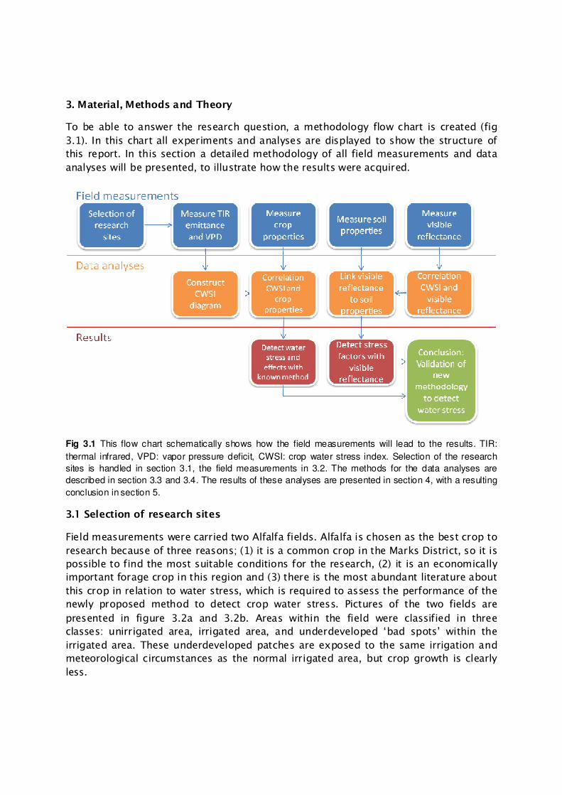
3. Material, Methods and Theory

To be able to answer the research question, a methodology flow chart is created (fig

3.1). In this chart all experiments and analyses are displayed to show the structure of

this report. In this section a detailed methodology of all field measurements and data

analyses will be presented, to illustrate how the results were acquired.

Fig 3.1 This flow chart schematically shows how the field measurements will lead to the results. TIR:

thermal infrared, VPD: vapor pressure deficit, CWSI: crop water stress index. Selection of the research

sites is handled in section 3.1, the field measurements in 3.2. The methods for the data analyses are

described in section 3.3 and 3.4. The results of these analyses are presented in section 4, with a resulting

conclusion in section 5.

3.1 Selection of research sites

Field measurements were carried two Alfalfa fields. Alfalfa is chosen as the best crop to

research because of three reasons; (1) it is a common crop in the Marks District, so it is

possible to find the most suitable conditions for the research, (2) it is an economically

important forage crop in this region and (3) there is the most abundant literature about

this crop in relation to water stress, which is required to assess the performance of the

newly proposed method to detect crop water stress. Pictures of the two fields are

presented in figure 3.2a and 3.2b. Areas within the field were classified in three

classes: unirrigated area, irrigated area, and underdeveloped ‘bad spots’ within the

irrigated area. These underdeveloped patches are exposed to the same irrigation and

meteorological circumstances as the normal irrigated area, but crop growth is clearly

less.

The two selected Alfalfa fields are about 40 kilometers apart, both in the Marks district

in Saratov region. The research sites will be referred to as field A (N51°49'46.85"

E47°05'32.53") and field B (N51°38'33.40" E46°45'19.66"). It was suspected from

satellite images that salt concentrations at these two fields differ, which is interesting

for this research. This way the influence of salinity and/or alkalinity properties on CWSI

could be studied. Field B was supposed to suffer from alkalinity problems, while field A

was located outside this alkanized patch. In section 2, pictures were presented of the

fields, with the difference between A1, A2 and A3, and B1 and B2. Several

measurements were conducted at these sites, 5 plots at field A, and 4 plots at field B.

At all these plots the same measurements are done. In table 3.1 the properties of the

plots are explained, in figure 3.3a and 3.3b pictures of the plots are presented.

Fig 3.2a. 3 different spots on alfalfa field A were selected; one irrigated, one non irrigated and one spot

with bad growing underdeveloped vegetation in the irrigated area.

Fig 3.2b. 2 different spots were selected on alfalfa field B; one irrigated and one spot with bad growing

underdeveloped vegetation.

Sample name Date Description Alfalfa field A: N51° 49' 46.85" E47° 05' 32.53" A1-1 6-july Unirrigated area, outside pivot system

A2-1 11-july Irrigated area, inside pivot system

A2-2 20-july Similar to spot A2-1, different date

A3-1 13-july Irrigated area, but poor crop quality

A3-2 20-july Similar to spot A3-1, different date Alfalfa field B: N51° 38' 33.40" E46° 45' 19.66" B1-1 9-july Irrigated area, but poor crop quality

B1-2 16-july Similar to spot B1-1, different date

B2-1 9-july Irrigated area, inside pivot system

B2-2 16-july Similar to spot B2-1, different date Table 3.1 this table summarizes plot description and date of measurement

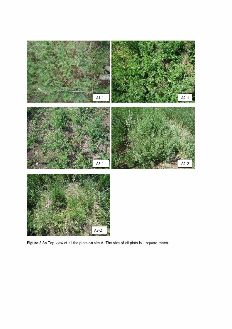
Figure 3.3a Top view of all the plots on site A. The size of all plots is 1 square meter.

A2-1 A1-1

A2-2 A3-1

A3-2

Figure 3.3b of all the plots on site B. All plots are 1 square meter.

3.2 Field measurements

At all 1 square meter plots, measurements are taken in four categories: meteorological

measurements, plant physiology, soil condition and remote sensing measurements.

3.2.1 Remote sensing measurements

Thermal infrared (TIR) emittance / canopy temperature. This parameter was measured because it is an important factor to determine the crop water stress index (CWSI) that will be explained in section 3.3. TIR emittance of the Alfalfa leaves is measured with the Raytek Raynger ST-20Pro, (details on www.raytek.com). This device measures TIR emittance as radiant temperature in degrees Celsius. To determine canopy temperature of a plot, a minimum of 2 series of measurements were taken, both series consisting of measurements from all wind directions under a 45º angle. So a minimum of 8 TIR measurements was done to determine canopy temperature. To prevent measuring soil temperature trough the leaves, it was made sure that no bare soil emittance was pickup up by holding the stems of vegetation together. Since this is a remote sensing technique, it is non-destructive, and if time allowed it, multiple measurements were taken at the same locations. In total 18 of these measurements were carried out.

B1-2 B1-1

B2-2 B2-1

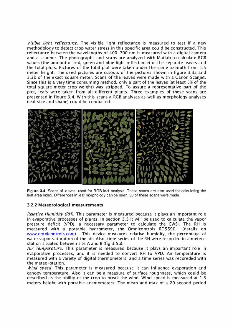
Visible light reflectance. The visible light reflectance is measured to test if a new methodology to detect crop water stress in this specific area could be constructed. This reflectance between the wavelengths of 400-700 nm is measured with a digital camera and a scanner. The photographs and scans are analyzed with Matlab to calculate RGB values (the amount of red, green and blue light reflectance) of the separate leaves and the total plots. Pictures of the total plot were taken under the same azimuth from 1.5 meter height. The used pictures are cutouts of the pictures shown in figure 3.3a and 3.3b of the exact square meter. Scans of the leaves were made with a Canon Scanjet. Since this is a very time consuming method, only a part of the leaves (at least 5% of the total square meter crop weight) was stripped. To assure a representative part of the plot, leafs were taken from all different plants. Three examples of these scans are presented in figure 3.4. With this scans a RGB analyses as well as morphology analyses (leaf size and shape) could be conducted.

Figure 3.4. Scans of leaves, used for RGB leaf analysis. These scans are also used for calculating the leaf area index. Differences in leaf morphology can be seen. 50 of these scans were made.

3.2.2 Meteorological measurements

Relative Humidity (RH). This parameter is measured because it plays an important role in evaporative processes of plants. In section 3.3 it will be used to calculate the vapor pressure deficit (VPD), a necessary parameter to calculate the CWSI. The RH is measured with a portable hygrometer, the Omnicontrols RD5590 (details on www.omnicontrols.com) . This device measures relative humidity, the percentage of water vapor saturation of the air. Also, time series of the RH were recorded in a meteo-station situated between site A and B (fig 3.5b). Air Temperature. This parameter is measured because it plays an important role in evaporative processes, and it is needed to convert RH to VPD. Air temperature is measured with a variety of digital thermometers, and a time series was recoreded with the meteo-station. Wind speed. This parameter is measured because it can influence evaporation and canopy temperature. Also it can be a measure of surface roughness, which could be described as the ability of the crop to break the wind. Wind speed is measured at 1.5 meters height with portable anemometers. The mean and max of a 20 second period

was determined, and a time series was recorded with the meteo-station. These values will be used to explain unexpected values for evaporation. 3.2.3. Plant physiology

Number of plants on the plot. All plants on the plot were counted since this parameter could give a response to water stress or soil properties. Mean height of the vegetation. Height of the five highest plants was measured, because it could give a response to water stress. The five highest plants were measured because measuring all plants was too time consuming, and this way a consequent and comparable mean was recorded. Dry and fresh biomass. Biomass is an important parameter to measure because it is the product that farmers harvest. With Alfalfa the total biomass is the yield, since the entire plants are used for forage purposes. All biomass of the square meter plots was harvested, stored, and weighted on the end of the field day on a digital weight scale. After weighing the biomass was dried in an oven at 80ºC for 24 hour and weighted again. Leaf area index (LAI). Leaf area could be an indicator for water stress since it is the

evaporative surface of the plant. Leaf area can be roughly estimated from pictures, but also a more detailed analysis is done, using the scans made for the analysis of visible light reflectance. The leaf scans (fig 3.4 and 3.5b) were converted to black and white pictures. All non white pixels in the scan are summed and converted to square centimeter leaf area in Matlab. This analysis is also conducted on a minimum of 5% of representative leaves, and extrapolated for the whole square meter. By dividing the LAI with the weight of the leafs the specific leaf area (SLA) is obtained.

3.2.4 Soil condition

Soil moisture (SM) of the upper soil. One of the most important factors controlling water stress is the amount of available water in the soil. We measure soil water content with the Trime FM (www.imko.de). At every spot 10 vertical measurements were taken, with a two rod probe. The device measures soil moisture as a percentage of saturation. Mean SM of these measurements is calculated for all plots. pH. pH is measured at every plot, to explore a possibility to detect the influence of

stress factors on the visible light reflectance. A high pH could be a signal of alkalinization. The pH was measured with a digital pH meter of Hanna instruments (www.hannainst.com). For these measurements, two samples were taken from the top soil, and three samples in a depth profile at 20cm, 40cm and 60cm depth. 20 grams of sediment were mixed with 20ml of demilitarized water (fig 3.5a). The suspensions were shaken intensively 3 times within an hour, and then the pH meter was inserted to check the acidity of the suspension. EC (Electric conductivity). The EC of the samples was checked to determine the amount of salts in the sediment. With this parameter it could be checked if the plot suffers from salinization issues. The methodology for determining EC was the same as for the pH, but a Hanna TDS (total dissolved solids) meter was used, and the suspension was shaken 3 more times to be sure all salts were dissolved. To convert the TDS to EC in KS/cm it had to be multiplied by two. Soil description. Visual signs of alkalinization or salinization are reported for every plot.

Also a general description of the soils is provided for both Alfalfa fields.

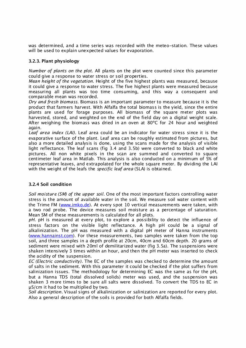
Fig 3.5 a (left), b (middle) and c (right). (a) some of the soil samples with 20 ml of water for the pH

and EC analyses. (b) Scanning leaves for LAI and RGB analyses. (c) The meteo station, positioned

between field A and B.

3.3 Determining Crop Water stress

Non-stressed crops open their stomata during the day for gas exchange, assimilating

carbon dioxide. While stomata are open, water can evaporate through these stomata.

Plants growing in conditions without sufficient available water tend to close their

stomata, to preserve the leaf water status (Chaves et al, 2002). Closing of the stomata

decreases the amount of carbon assimilation (photosynthesis), and thus decreases

plant growth (Jackson, 1981).

Under non-stressed conditions stomata are open and plants transpire. This causes the

leaves to be cooler then the surrounding air, because available radiation converts to

latent heat. The reduction in transpiration due to water shortage has an effect on the

leaf temperature, since incoming radiation does not convert to latent heat but to

sensible heat. This principle is the basis for a much-used way to detect water stress;

the difference between canopy and air temperatures (Tc – T

a) decreases when stomata

are closed (Idso and Jackson et al, 1981). Tc is measured with the thermal infrared

sensor. The amount of incoming solar radiation should be maximal, since higher

radiation is believed to maximize the empirical relation (Payero, 2005).

The crop water stress is also dependent on the vapor pressure deficit (VPD). The VPD

indicates how far the air is from saturation with water vapor at a specific air

temperature. The VPD can be calculated from the relative humidity (RH) measurements,

combined with air temperature measurements. This is done with a series of formulas.

The VPD is the saturation vapor pressure at a certain temperature minus the actual

vapor pressure. This is show in formula 3.3.1.

VPD = e*(T) – e(T) (formula 3.3.1)

Where e*(T) = saturation vapor pressure, e(T) = water vapor pressure in hPa.

Subsequently, e*(T) is calculated with formula 3.3.2 and e(T) is calculated with formula

3.3.3

e*(T) = 6.112e 17.67(T−273.15)/ (T−29.65) (formula 3.3.2)

Where T = temperature in degrees Kelvin.

e(T) = RH * e*(T) (formula 3.3.3)

Where RH = relative humidity (percentage/100).

When the vapor pressure deficit is low, less evaporation will take place, which will

influence Tc – T

a. Idso (1981) Jackson (1981) and Hatfield (1993) used the relation

between VPD and Tc – T

a to determine if a crop is in water stress. They discovered that

all points in a scatter plot of Tc – T

a as a function of VPD ranged between a non-

stressed baseline and a maximal stressed upper line.

These limits are empirically determined for every crop. This is done by monitoring well

watered plants without water stress, and non-transpiring plants (dead plants) in a

controlled setup. These plants are the so called control plots. In figure 3.6, adapted

from Idso and Jackson et al, 1981 the empirically derived baseline and upper line are

illustrated. It is visible that although the studies were done at different dates and

locations, plotting the measurements of the non-stressed observations all fall on the

same line. Slight variation can occur as discovered by Payero, 2005, as a result of

surface roughness, wind speed and the intensity of solar radiation. Therefore, for every

study a new emperical relation is found, as for this study.

Figure 3.6 illustrates research done in four different states in the USA. As described,

the baseline represents vegetation without any water stress. The upper line represents

non-transpiring vegetation in maximum water stress. All measurements should lie

between these two line. The exact position of a certain measurements between these

two lines determines the amount of stress the crop is in. This is called the crop water

stress index (CWSI), a value between 0 and 1 where 0 is on the baseline and 1 is on the

upper line . This value of CWSI is calculated with formula 3.3.4.

CWSI = ������ ��������� �

������ ��������� � (formula 3.3.4)

Where p = point of measurement, bl = base line and ul = upper line.

Examples of the ‘point of measurement’ mentioned in formula 3.3.4 are illustrated in

figure 3.5 as point A, point B and point C. These are 3 hypothetical measurements of

(Tc – T

a)p and VPD of a crop at a certain plot. Because point A is almost on the upper

line, (Tc – T

a)p O (T

c – T

a)ul so the CWSI O 1 (maximum water stress). Point C is almost on

the baseline, so (Tc – T

a)p O (T

c – T

a)bl so that CWSI O 0 (minimum water stress). Point B is

exactly between the two lines, so CWSI = 0.5.

Figure 3.6. CWSI diagram, with 3 hypothetical measurements. Point A is in severe water stress

because CWSI is around 1, point B suffers water stress with a CWSI of 0.5, and point C does not

suffer from any water stress, so CWSI is close to 0. Figure adapted from Idso and Jackson et al,

1981.

The baseline for this study was constructed along results of the best irrigated plots of

our study, A2 and B2. Measurements taken with higher wind speeds were given less

significance in constructing the baseline. Also literature was studied to construct the

best suitable baseline. The upper line was constructed above the measurement outside

the irrigation pivot system, with the lowest SM, at plot A1-1. It is important to note that

the CWSI is a momentary measurement; CWSI on a plot can differ during the day

because of water application, rain and meteorological circumstances on a specific time

of the day. This is illustrated for two plots in fig 3.7.

3.4 Correlation and links between parameters

After the crop water stress index was calculated for all plots, it was correlated with the

crop physiology, to check if the CWSI of the plots had a direct link with the plant

physiological properties (explained in section 3.2.3). CWSI is a momentary

measurement which can change during the day (fig 3.7) because the index is

dependent on time of irrigation and meteorological circumstances. Therefore every

field day, sets of two measurements (e.g. B1-1 and B2-1) were taken on the same day,

around the same time, to be able to compare them. The same applies for soil moisture

in the top soil. Properties like LAI, biomass and the amount and height of plants show

less daily variability. It would be ideal to have a time series of CWSI measurement

through the whole growing season, and then correlate the mean water stress index of

the whole season with physiological properties. During this fieldwork there was no time

to do an analysis like this; all physiology measurements of different vegetation types

could just be measured two times, except for A1 that was measured only one time.

Still correlations can be made on the assumption that the crops on non irrigated plots

suffer more water stress then irrigated crops. Also the underdeveloped bad spots (fig

3.2 and 3.2b) in the irrigated area are assumed to be in more stress then crops growing

in more healthy conditions. These assumptions will be tested with the 18 CWSI

measurements that are conducted. CWSI measurements from the different locations

(A1, B1 and A3 vs. A2 and B2) are compared with a Man Whitney U-test to test if the

group medians differ significantly, as done by Barbosa da Silva et al, 2005. Sets of CWSI

measurements were carried out on the same day, around the same time, so results are

comparable. When there seems to be a significant difference in CWSI between the plots,

the relation between crop physiology and crop water stress will be studied using the

same two sets of plots. Since crop water stress has an influence on the amount of

carbon fixation, a relation with crop physiology is not unlikely.

Besides the physiological effects of crop water stress, also the effect of soil quality, and

water availability on crop water stress were established. For water availability this was

done by conducting a regression analyses comparing CWSI with soil moisture, since

both variables are momentary measurements. pH and EC were correlated with the

physiological parameters via a regression analysis, to research the influence of these

factors on plant growth and morphology.

Fig. 3.7. CWSI of two plots (stressed and not stressed), from a study of Barbosa de Silva et al, 2005 in

Brazil. As can be seen, CWSI is a momentary measurement, and changes significantly during a day.

Therefore it can be correlated with other temporal measurements like soil moisture, but not so easily with

more stable parameters like pH.

As explained in section 3.2.1, 50 high resolution full color scans were made of leaves

from the 9 different plots. These scans were also converted for use for LAI calculation.

The RGB analysis conducted on these scans is correlated to the plant physiology and

soil properties, via a regression analyses, and mean RGB values of plots with different

soil properties are compared with a T-test.

The digital pictures of the plots were also analyzed using a RGB analysis. By looking at

the individual red, green and blue bands, and the ratio between them, correlations

between CWSI and soil properties with these RGB values were studied, using a

regression analysis. By using ratios between different color bands, external factors (like

scattering and the amount of solar radiation) were tried to be eliminated to a maximum

amount. The ratios between green and blue reflectance, and green and red reflectance

were selected because this is a measure for the amount of chlorophyll absorption,

which takes place at a wavelength of 44Km (blue) and 65Km (red) (Jensen, 2000).

Chlorophyll concentration in leaves is a common indicator for plant health.

While leaf RGB analyses (fig 3.4) most probably will not correlate with the CWSI, since

the CWSI values are a momentary measurement, the RGB values of the total plots (like

fig 3.3a and 3.3b) might correlate better with CWSI, because wilking plants cast

different shadow patterns, and plant water content can change the plant’s color.

4. Results

All experiments were executed successfully, except for the dry biomass weighing,

because two key samples seemed to have burned in the oven, after soil scientist

colleges altered the temperature for soil sample drying. All results are summarized in

tables 4.1, 4.4 and 4.6.

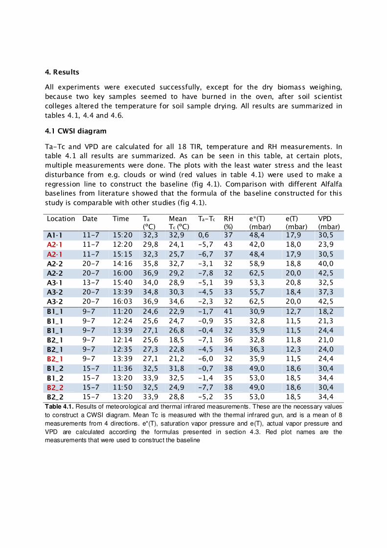
4.1 CWSI diagram

Ta-Tc and VPD are calculated for all 18 TIR, temperature and RH measurements. In

table 4.1 all results are summarized. As can be seen in this table, at certain plots,

multiple measurements were done. The plots with the least water stress and the least

disturbance from e.g. clouds or wind (red values in table 4.1) were used to make a

regression line to construct the baseline (fig 4.1). Comparison with different Alfalfa

baselines from literature showed that the formula of the baseline constructed for this

study is comparable with other studies (fig 4.1).

Location Date Time Ta (ºC)

Mean Tc (ºC)

Ta-Tc RH (%)

e*(T) (mbar)

e(T) (mbar)

VPD (mbar)

A1-1 11-7 15:20 32,3 32,9 0,6 37 48,4 17,9 30,5

A2-1 11-7 12:20 29,8 24,1 -5,7 43 42,0 18,0 23,9

A2-1 11-7 15:15 32,3 25,7 -6,7 37 48,4 17,9 30,5

A2-2 20-7 14:16 35,8 32,7 -3,1 32 58,9 18,8 40,0

A2-2 20-7 16:00 36,9 29,2 -7,8 32 62,5 20,0 42,5

A3-1 13-7 15:40 34,0 28,9 -5,1 39 53,3 20,8 32,5

A3-2 20-7 13:39 34,8 30,3 -4,5 33 55,7 18,4 37,3

A3-2 20-7 16:03 36,9 34,6 -2,3 32 62,5 20,0 42,5

B1_1 9-7 11:20 24,6 22,9 -1,7 41 30,9 12,7 18,2

B1_1 9-7 12:24 25,6 24,7 -0,9 35 32,8 11,5 21,3

B1_1 9-7 13:39 27,1 26,8 -0,4 32 35,9 11,5 24,4

B2_1 9-7 12:14 25,6 18,5 -7,1 36 32,8 11,8 21,0

B2_1 9-7 12:35 27,3 22,8 -4,5 34 36,3 12,3 24,0

B2_1 9-7 13:39 27,1 21,2 -6,0 32 35,9 11,5 24,4

B1_2 15-7 11:36 32,5 31,8 -0,7 38 49,0 18,6 30,4

B1_2 15-7 13:20 33,9 32,5 -1,4 35 53,0 18,5 34,4

B2_2 15-7 11:50 32,5 24,9 -7,7 38 49,0 18,6 30,4

B2_2 15-7 13:20 33,9 28,8 -5,2 35 53,0 18,5 34,4

Table 4.1. Results of meteorological and thermal infrared measurements. These are the necessary values

to construct a CWSI diagram. Mean Tc is measured with the thermal infrared gun, and is a mean of 8

measurements from 4 directions. e*(T), saturation vapor pressure and e(T), actual vapor pressure and

VPD are calculated according the formulas presented in section 4.3. Red plot names are the

measurements that were used to construct the baseline

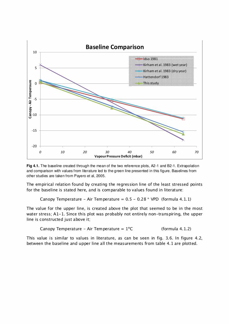
Fig 4.1. The baseline created through the mean of the two reference plots, A2-1 and B2-1. Extrapolation

and comparison with values from literature led to the green line presented in this figure. Baselines from

other studies are taken from Payero et al, 2005.

The empirical relation found by creating the regression line of the least stressed points

for the baseline is stated here, and is comparable to values found in literature:

Canopy Temperature - Air Temperature = 0.5 - 0.28 * VPD (formula 4.1.1)

The value for the upper line, is created above the plot that seemed to be in the most

water stress; A1-1. Since this plot was probably not entirely non-transpiring, the upper

line is constructed just above it;

Canopy Temperature - Air Temperature = 1ºC (formula 4.1.2)

This value is similar to values in literature, as can be seen in fig. 3.6. In figure 4.2,

between the baseline and upper line all the measurements from table 4.1 are plotted.

-20

-15

-10

-5

0

5

10

0 10 20 30 40 50 60 70

Ca

no

py

-A

ir T

em

pe

rau

re

Vapour Pressure Deficit (mbar)

Baseline Comparison

Idso 1981

Kirham et al. 1983 (wet year)

Kirham et al. 1983 (dry year)

Hattendorf 1983

This study

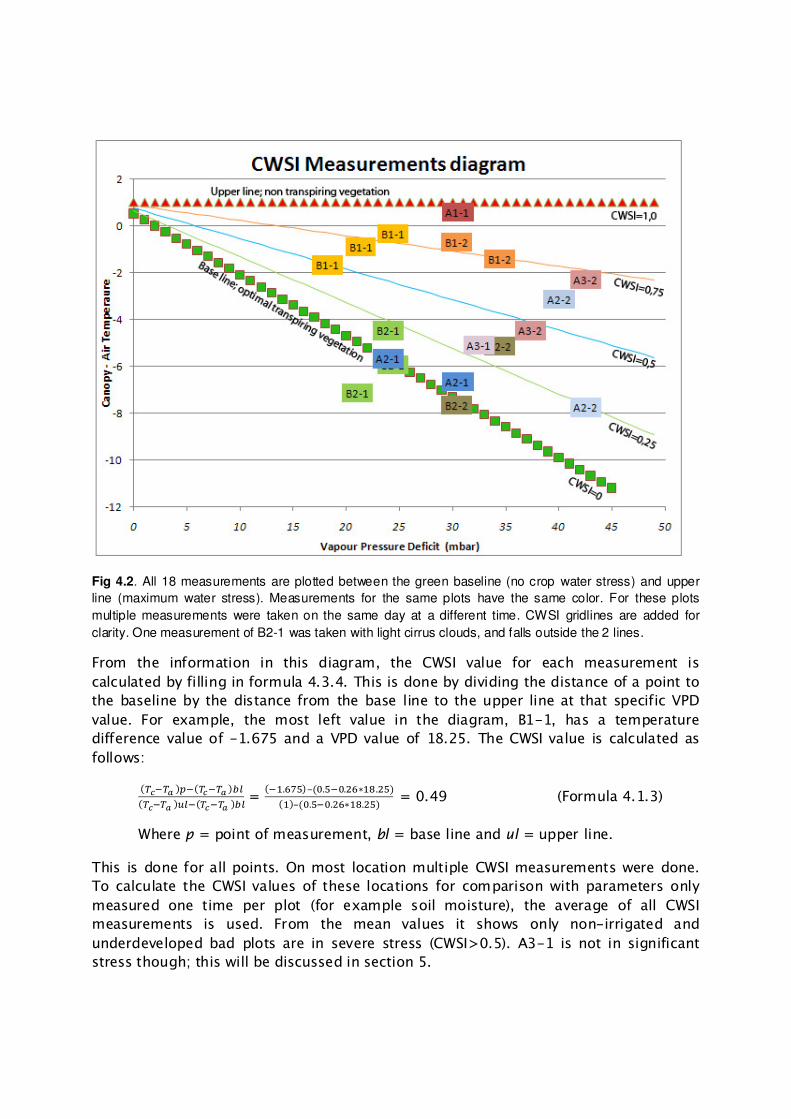
Fig 4.2. All 18 measurements are plotted between the green baseline (no crop water stress) and upper

line (maximum water stress). Measurements for the same plots have the same color. For these plots

multiple measurements were taken on the same day at a different time. CWSI gridlines are added for

clarity. One measurement of B2-1 was taken with light cirrus clouds, and falls outside the 2 lines.

From the information in this diagram, the CWSI value for each measurement is

calculated by filling in formula 4.3.4. This is done by dividing the distance of a point to

the baseline by the distance from the base line to the upper line at that specific VPD

value. For example, the most left value in the diagram, B1-1, has a temperature

difference value of -1.675 and a VPD value of 18.25. The CWSI value is calculated as

follows:

������ ��������� �

������ ��������� � =

���.����–��.���.�����.���

���–��.���.�����.��� = 0.49 (Formula 4.1.3)

Where p = point of measurement, bl = base line and ul = upper line.

This is done for all points. On most location multiple CWSI measurements were done.

To calculate the CWSI values of these locations for comparison with parameters only

measured one time per plot (for example soil moisture), the average of all CWSI

measurements is used. From the mean values it shows only non-irrigated and

underdeveloped bad plots are in severe stress (CWSI>0.5). A3-1 is not in significant

stress though; this will be discussed in section 5.

Field A CWSI Field B CWSI

A1_1 0,95 B1_1 0,66

A2_1 0,05 B1_2 0,77

A2_2 0,43 B2_1 -0,06

A3_1 0,32 B2_2 0,16

A3_2 0,59

Table 4.2. Mean CWSI of plots for comparison with

other measurements. Plots with red values have

CWSI values above 0.5, and are in severe water

stress.

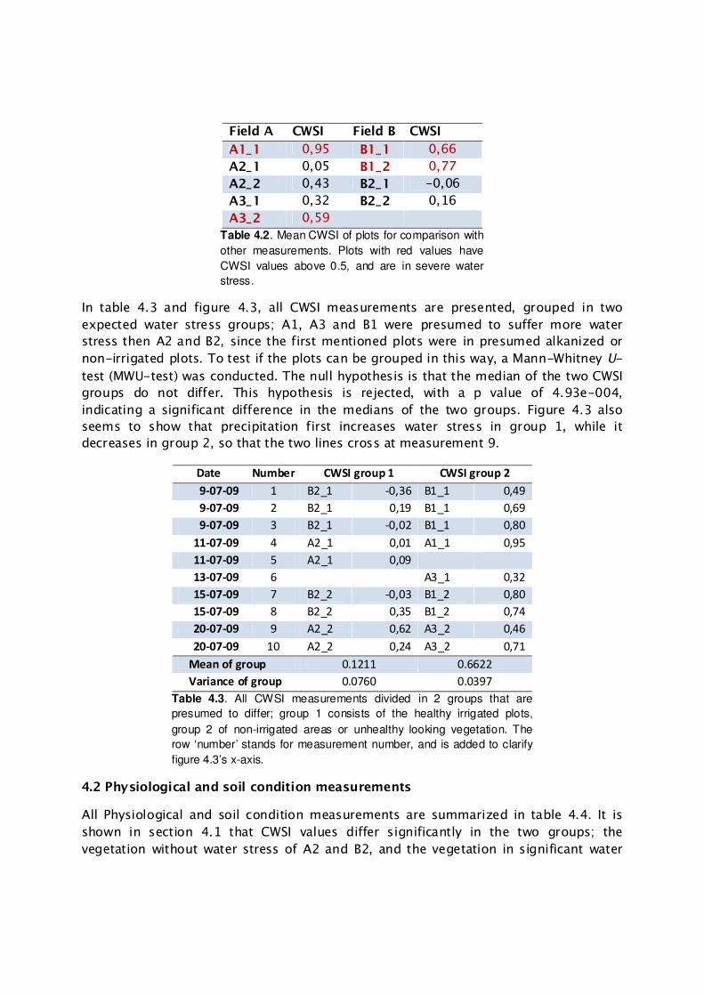
In table 4.3 and figure 4.3, all CWSI measurements are presented, grouped in two

expected water stress groups; A1, A3 and B1 were presumed to suffer more water

stress then A2 and B2, since the first mentioned plots were in presumed alkanized or

non-irrigated plots. To test if the plots can be grouped in this way, a Mann-Whitney U-

test (MWU-test) was conducted. The null hypothesis is that the median of the two CWSI

groups do not differ. This hypothesis is rejected, with a p value of 4.93e-004,

indicating a significant difference in the medians of the two groups. Figure 4.3 also

seems to show that precipitation first increases water stress in group 1, while it

decreases in group 2, so that the two lines cross at measurement 9.

Date Number CWSI group 1 CWSI group 2

9-07-09 1 B2_1 -0,36 B1_1 0,49

9-07-09 2 B2_1 0,19 B1_1 0,69

9-07-09 3 B2_1 -0,02 B1_1 0,80

11-07-09 4 A2_1 0,01 A1_1 0,95

11-07-09 5 A2_1 0,09

13-07-09 6 A3_1 0,32

15-07-09 7 B2_2 -0,03 B1_2 0,80

15-07-09 8 B2_2 0,35 B1_2 0,74

20-07-09 9 A2_2 0,62 A3_2 0,46

20-07-09 10 A2_2 0,24 A3_2 0,71

Mean of group 0.1211 0.6622

Variance of group 0.0760 0.0397

Table 4.3. All CWSI measurements divided in 2 groups that are

presumed to differ; group 1 consists of the healthy irrigated plots,

group 2 of non-irrigated areas or unhealthy looking vegetation. The

row ‘number’ stands for measurement number, and is added to clarify

figure 4.3’s x-axis.

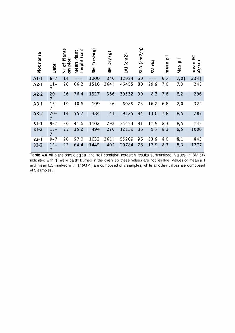
4.2 Physiological and soil condition measurements

All Physiological and soil condition measurements are summarized in table 4.4. It is

shown in section 4.1 that CWSI values differ significantly in the two groups; the

vegetation without water stress of A2 and B2, and the vegetation in significant water

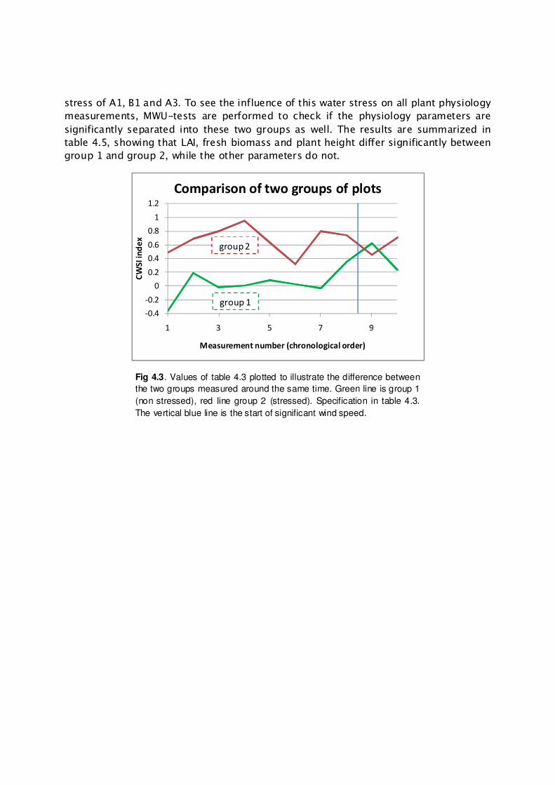
stress of A1, B1 and A3. To see the influence of this water stress on all plant physiology

measurements, MWU-tests are performed to check if the physiology parameters are

significantly separated into these two groups as well. The results are summarized in

table 4.5, showing that LAI, fresh biomass and plant height differ significantly between

group 1 and group 2, while the other parameters do not.

Fig 4.3. Values of table 4.3 plotted to illustrate the difference between

the two groups measured around the same time. Green line is group 1

(non stressed), red line group 2 (stressed). Specification in table 4.3.

The vertical blue line is the start of significant wind speed.

-0.4

-0.2

0

0.2

0.4

0.6

0.8

1

1.2

1 3 5 7 9

CW

SI

ind

ex

Measurement number (chronological order)

Comparison of two groups of plots

group 2

group 1

Plot name

Date

Nr of Plants

on plot

Mean Plant

Height (cm)

BM Fresh(g)

BM Dry (g)

LAI (cm2)

SLA (cm2/g)

SM (%)

mean pH

Max pH

mean EC

µS/cm

A1-1 6-7 14 --- 1200 340 12954 60 --- 6,7‡ 7,0‡ 234‡

A2-1 11-7

26 66,2 1516 264† 46455 80 29,9 7,0 7,3 248

A2-2 20-7

26 76,4 1327 386 39532 99 8,3 7,6 8,2 296

A3-1 13-7

19 40,6 199 46 6085 73 16,2 6,6 7,0 324

A3-2 20-7

14 55,2 384 141 9125 94 13,0 7,8 8,5 287

B1-1 9-7 30 41,6 1102 292 35454 91 17,9 8,3 8,5 743

B1-2 15-7

25 35,2 494 220 12139 86 9,7 8,3 8,5 1000

B2-1 9-7 20 57,0 1633 261† 55209 96 33,9 8,0 8,1 843

B2-2 15-7

22 64,4 1445 405 29784 76 17,9 8,3 8,3 1277

Table 4.4 All plant physiological and soil condition research results summarized. Values in BM dry

indicated with ‘†’ were partly burned in the oven, so these values are not reliable. Values of mean pH

and mean EC marked with ‘‡’ (A1-1) are composed of 2 samples, while all other values are composed

of 5 samples.

parameter Mean group 1

Mean group 2

p H0

rejected Nr of Plants on plot 23.5 20.4 0.3968 no

Mean Plant Height (cm) 66.0 43.2 0.0286 yes

Biomass Fresh (g) 1480 676 0.0159 yes

Biomass Dry (g) 329 208 0.1905 no

LAI (cm2) 42745 15151 0.0317 yes

SLA (cm2/g) 87.8 80.8 0.4127 no

Table 4.5. In this table the results of MWU-tests are summarized comparing the crops with

plants in good state (group 1) and in bad, underdeveloped state (group 2). For some

physiology properties this same categorization as for CWSI is significant. These physiological

properties could be caused by crop water stress.

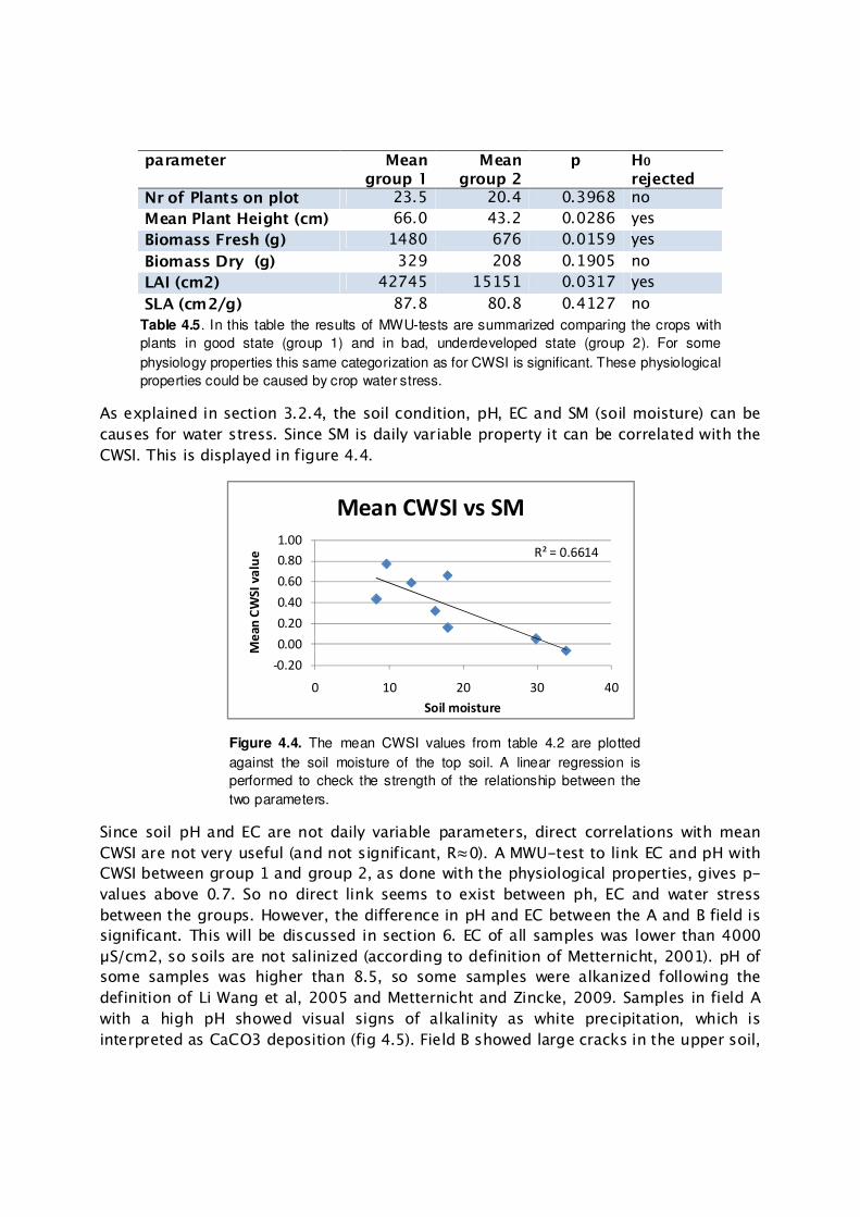
As explained in section 3.2.4, the soil condition, pH, EC and SM (soil moisture) can be

causes for water stress. Since SM is daily variable property it can be correlated with the

CWSI. This is displayed in figure 4.4.

Figure 4.4. The mean CWSI values from table 4.2 are plotted

against the soil moisture of the top soil. A linear regression is

performed to check the strength of the relationship between the

two parameters.

Since soil pH and EC are not daily variable parameters, direct correlations with mean

CWSI are not very useful (and not significant, RO0). A MWU-test to link EC and pH with

CWSI between group 1 and group 2, as done with the physiological properties, gives p-

values above 0.7. So no direct link seems to exist between ph, EC and water stress

between the groups. However, the difference in pH and EC between the A and B field is

significant. This will be discussed in section 6. EC of all samples was lower than 4000

KS/cm2, so soils are not salinized (according to definition of Metternicht, 2001). pH of

some samples was higher than 8.5, so some samples were alkanized following the

definition of Li Wang et al, 2005 and Metternicht and Zincke, 2009. Samples in field A

with a high pH showed visual signs of alkalinity as white precipitation, which is

interpreted as CaCO3 deposition (fig 4.5). Field B showed large cracks in the upper soil,

R² = 0.6614

-0.20

0.00

0.20

0.40

0.60

0.80

1.00

0 10 20 30 40

Me

an

CW

SI

va

lue

Soil moisture

Mean CWSI vs SM

which is interpreted as a sign of alkalinization or drought (Metternicht and Zinck,

2009). pH’s of 8,5 only seem to occur in the plots that are in group 2, but the

differences are very small; the pH in the group 1 plots reach up to 8,3.

Fig 4.5. Signs of alkalinity on field A (assumed precipitation of CaCO3. And field B (mudcracks).

4.3 Visible light remote sensing

In this section the results are presented of VIS (visible light reflectance) analyses of two

experiments; the leaf scans and the plot picture analyses.

The mean red, green and blue values of the 50 leaf scans are displayed in Table 4.6.

There does not seem to be a correlation between measured CWSI and the scanned leaf

color. A theory was that plant water content might influence the leaf color, but since

the scans are made around 5 hours after harvesting the plant this influence might be

less. Also, this effect of water content is only known in literature from reflectance, and

in the scanner there is no real sunlight reflectance. However, there seems to be a

difference in leaf color (especially in the green band) between the A and B field, and

since pH and EC differ significantly at both fields as well, the relation between the

green band with pH and EC is plotted in figure 4.6a and 4.6b. Replacing the green with

the red band gives a similar picture, while the blue band doesn’t seem to correlate with

pH and EC. A t-test to compare leaf green values of the 50 scans of field A and field B

points out significant differences between the fields (p<0,01). The same applies for the

leaf red values, but not for the blue values. Field B has a higher EC and pH, and lighter

colored leaves, since both green and red values are higher and blue values are the

same. Anthocyanins are pigments that are known to have different colors when soil pH

varies (Kong et al, 2003). These pigments might be responsible for the difference in

leaf color between the two fields.

Leaf scan analysis Plot picture color ratios

Red Green Blue Red/Green Blue/Green

A1-1 96 101 80 0,84 0,69

A2-1 94 102 74 0,7 0,51

A2-2 97 104 77 0,79 0,63

A3-1 95 102 78 0,85 0,72

A3-2 103 108 79 0,86 0,67

Mean A 93 103 78

B1-1 103 110 76 0,83 0,71

B1-2 116 116 89 0,94 0,73

B2-1 105 116 71 0,71 0,53

B2-2 103 111 75 0,68 0,48

Mean B 107 113 78

Table 4.6 Visible light RGB analysis results of leaf scans and plot pictures. All

leaf scan RGB values are means of several scans of the same plot. For the leaf

scan analysis, a mean of the fields is also calculated to underline the difference

between the fields.

Fig 4.6a (left) and b (right). The mean green values of the scans seem to have a strong relation to

pH and EC.

The RGB values of the plot pictures are expressed in ratios (table 4.6). The red/green

and blue/green ratios were observed to relate to the CWSI measurements (fig 4.7a and

b). The CWSI index increases with increasing ratios of mean red/green and blue/green.

These ratios can be a measure of the amount of absorption of the pigment chlorophyll,

since chlorophyll absorbs light in the red and blue areas of the electromagnetic

spectrum (as explained in section 3.4).

R² = 0.7605

6.00

6.507.007.50

8.008.509.00

100 105 110 115 120

pH

mean green value of leaf scan

pH vs Leaf GreenR² = 0.6624

0

500

1000

1500

100 105 110 115 120

EC

mean green value of leaf scan

EC vs Leaf Green

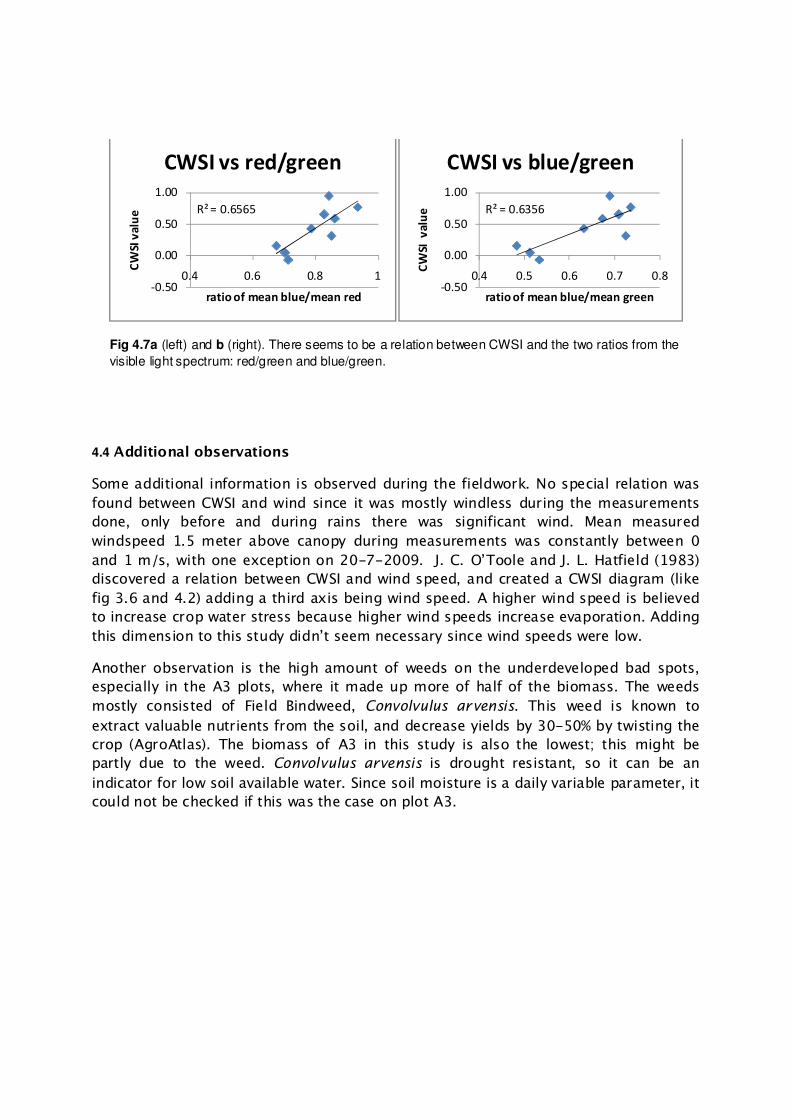
Fig 4.7a (left) and b (right). There seems to be a relation between CWSI and the two ratios from the

visible light spectrum: red/green and blue/green.

4.4 Additional observations

Some additional information is observed during the fieldwork. No special relation was

found between CWSI and wind since it was mostly windless during the measurements

done, only before and during rains there was significant wind. Mean measured

windspeed 1.5 meter above canopy during measurements was constantly between 0

and 1 m/s, with one exception on 20-7-2009. J. C. O’Toole and J. L. Hatfield (1983)

discovered a relation between CWSI and wind speed, and created a CWSI diagram (like

fig 3.6 and 4.2) adding a third axis being wind speed. A higher wind speed is believed

to increase crop water stress because higher wind speeds increase evaporation. Adding

this dimension to this study didn’t seem necessary since wind speeds were low.

Another observation is the high amount of weeds on the underdeveloped bad spots,

especially in the A3 plots, where it made up more of half of the biomass. The weeds

mostly consisted of Field Bindweed, Convolvulus arvensis. This weed is known to

extract valuable nutrients from the soil, and decrease yields by 30-50% by twisting the

crop (AgroAtlas). The biomass of A3 in this study is also the lowest; this might be

partly due to the weed. Convolvulus arvensis is drought resistant, so it can be an

indicator for low soil available water. Since soil moisture is a daily variable parameter, it

could not be checked if this was the case on plot A3.

R² = 0.6565

-0.50

0.00

0.50

1.00

0.4 0.6 0.8 1

CW

SI v

alu

e

ratio of mean blue/mean red

CWSI vs red/green

R² = 0.6356

-0.50

0.00

0.50

1.00

0.4 0.5 0.6 0.7 0.8

CW

SI

va

lue

ratio of mean blue/mean green

CWSI vs blue/green

5 Discussion and conclusions

By creating a CWSI diagram, it appeared that there was a significant difference in water

stress between the plots of group 1 and group 2. High CWSI values were found in

group 2, with the plants on presumed alkanized spots. The highest CWSI value was

measured for the non-irrigated plot, A1. The lowest CWSI values were those measured

in group 1, the irrigated plots without suspected alkalinity. It was shown that this stress

shows a relation to specific physiological parameters; the leaf area index, the fresh

biomass and the mean plant height. The mean plant height seemed to correlate well

with CWSI, and it is a very easy to measure parameter. It might be a good strategy to

develop a nominal plant height index schedule for non water stressed crops, to easily

detect if crops are not optimally growing, and might be in water stress. The relation

between CWSI and fresh biomass showed that research to water stress is useful, since it

has a direct link with the yield of Alfalfa.

Remote sensing of the visible light spectrum has shown to be an interesting tool to

determine plant properties. The leaf color of different crops on different plots appeared

to be correlated with pH and EC properties of the soil, especially within the green and

red band. It would be interesting to test this with more samples, and a larger range of

pH and EC values. Top view plot pictures also seemed to be of use in detecting crop

water stress. Correlating the visible light band ratios red/green and blue/green to CWSI

gave a good fit. The different reflection of stressed plants, and the amount of bare soil

seems to be representative for crop water stress. More research is necessary to prove if

this relation is applicable in different environments, and for different crops. Also, the

influence of crop age on this relation should be studied. If research points out that this

is possible, it could be a much easier way to determine crop water stress than with the

thermal gun. Also satellite images could be used to do these measurements, instead of

digital cameras. This would increase the spatial extent of this methodology.

Possible causes for the water stress were studied, like soil EC, pH and SM. It seems that

soil moisture in the upper soil has a big influence on the CWSI. This relation was

expected, because more soil moisture means more available water for the crop, so

more transpiration is possible. This is also why plot A2-2 has a relative high CWSI

value; soil moisture was very low because this measurement was taken in the longest

period of no rain. Also pivot irrigation was shut down for some days.

Less clear is the role of salinization and alkalinization in the two fields. Expected was

that plots A3 and B1 were spots with higher EC and/or higher pH, but this was not

uniformly the case. So the worse physiological parameters of group 2 cannot directly

be explained with alkalinity or salinity levels. Between fields A and B there is a

difference in pH and EC: field B had a higher value for both parameters. This could be

an indication for alkalinization in field B. EC values were too low to speak of salinized

soils, but there are samples that could be labeled as slightly alkalinized. Li Wang et al,

2005 and Metternicht and Zincke, 2009, defined alkaline soils as soils with pH>8.5 and

EC<4000KS/cm2. In all measurements of field A and B there were four samples at

different depths matching these criteria, but mean plot values of pH of all depths were

all lower than 8.5. Although not all bad plots have alkalinized spots, all the alkanized

spots seem to occur in bad plots (B1-1, B1-2 and A3-2). A1-1 is probably not

alkalinized because it is not irrigated. It is not clear why A3-1 has underdeveloped

vegetation since there seemed to be no alkalinity problems at all at this plot. It could be

possible that there are other problems at this spot, like soil compaction, nutrient

leaching, plant sickness, and the influence of weeds.

It is also possible that alkalinity problems only occur at higher depth. According to

Gabchenko et al, 2005, alkanized soils in southwest Russia have high carbonate

concentrations between 50-100cm and deeper, as illustrated in fig 5.1. More detailed

information and conclusions about soil condition and hydrology will be provided in the

paper of Jeremy Croes.

The high presence of Convolvulus arvensis is an indicator for a shortage of available

water. This could be caused by alkalinization, and can lead to more bare soil, since

plant growth is negatively affected. Bare soil is more sensitive to compaction, since

there is less biological activity. Also, nutrients can be washed out more easily. This land

degradation process is also a reason why salinization and/or alkalinization in the past

could have led to current bad soil conditions, and vegetation patterns. More chemical

analyses and soil science on the studied areas could provide more clarity on the

influence of alkalinity on crop water stress.

Fig 5.1. Carbonate levels of alkanized soils still rise

after 60cm, the maximum depth that was studied in

this study.

When, after more research, crop water stress will seem to be the effect of alkalinity or

nutrient leaching, experimentation with drip irrigation might be a wise strategy. This

can help preventing further land degradation, and is a solution for the water shortage

problems and the worsening condition of the irrigation systems. Drip irrigation is

currently tested as a strategy for sustainable land management in the area in the

framework of the DESIRE project.

The wind event on 20-07-2009 seemed to have increased water stress in group 1,

while it decreased water stress on group 2 during the wind event (fig 4.3). Two hours

later however, under the same meteorological circumstances, the effect on both groups

is reversed. It is assumable that wind disturbs CWSI measurements with TIR

measurements, since it has a temporal variation within seconds. A new methodology to

detect CWSI with VIS reflectance might provide a solution to this problem, since it is not

influenced by rapid variations of leaf temperature due to wind. The new methodology

could provide an easier to measure, and more stable index.

6. Acknowledgements

For me this was the most interesting and exciting study of my masters program. I

would like to thank Jeremy Croes, good friend and colleague, who chose to join me to

do his master thesis in Russia. To be able to get this opportunity I would like to thank

my supervisors: Simone Verzandvoort and Eli Argaman. They helped me with

constructive feedback, and field support in Russia.

I also like to thank our Russian colleagues and friends: Anatoly Zeiliguer, Olga

Ermolaeva, Vyacheslav Semenov, Oleg Karpenko, Alexey Teplov, Tatyana Petrovets, and

all other Employees at the Moscow State University of Environmental Engineering. They

welcomed us with great care and warmth, and supported us throughout the whole

fieldwork period. Also they taught us about the Russian language and culture, and

showed us so many interesting places I will never forget.

7. References

AgroAtlas http://www.agroatlas.ru/en/content/weeds/Convolvulus_arvensis/

B. Barbosa da Silva, T.V. Ramana Rao (2005). The CWSI variations of a cotton crop in a

semi-arid region of Northeast Brazil. Journal of Arid Environments vol 62, 649–659.

M.M. Chaves, J. S. Pereira, J. Maroco, M. L. Rodigues, C. P. P. Ricardo, M. L. Osorio, I.

Carvalho, T. Faria and C. Pinheiro (2003) How plants cope with water stress in the field?

Photosynthesis and Growth. Annals of Botany, vol 89. 907-916

DESIRE Project website: http://www.desire-project.eu

EEA report 2003 Europe’s environment: The third assessment. ISBN: 92-9167-574-1

FAO report 2008 http://www.fao.org/docrep/004/x3109e/pays/usr9909e.htm

M.V. Gabchenko (2008) Modern State of Soil Salinity in Solonetzic Soil Complexes

at the Dzhanybek Research Station in the North Caspian Region. Eurasian Soil

Science, vol 41, 360-370.

J.L. Hatfield et al (1993) Remote Sensing for crop protection. Crop Protection, vol 12,

403-413.

A. Iannucci, N. Di Fonzo, P. Martiniello (2002) Alfalfa (Medicago sativa L.) Seed yield and

quality under different forage management systems and irrigation treatments in a

Mediterranean environment, Field Crops Research, vol 78, 65-74.

S.B. Idso, R.D. Jackson, P.J. Pinter, Jr., R.J. Reginato and J.L. Hatfield (1981). Normalizing

the stress degree parameter for environmental variability. Agricultural Meteorology,

vol 24, 45-55

R.D. Jackson, S.B. Idso, R.J. Reginato, P.J. Jr. Pinter (1981) Canopy temperature as a

crop water stress indicator, Water Resources Research, vol 17, 1133-1138.

J.R. Jensen (2000) Remote Sensing of the Environment: An Earth Resource Perspective.

Prentice Hall, ISBN 0134897331

Kong JM, Chia LS, Goh NK, et al. (2003) Analysis and biological activities of

anthocyanins. Phytochemistry vol 64:923-933.

N.N. Ladonina, D.A. Cherniakhovsky, I.B. Makarov, V.F. Basevich (2001) Managing

Agricultural Resources for Biodiversity Conservation: Case study of Russia and CIS

countries, Environment Liaison Center International

Metternicht G (2001) Assessing temporal and spatial changes of salinity using fuzzy

logic, remote sensing and GIS Foundations of an expert system. Ecological Modeling

144:163–179.

Metternicht and Zinck, editors (2009). Remote Sensing of Soil Salinization: Impact on

Land Management. CRC press. ISBN: 978-1-4200-6502-2

S.L. O’Hara (1997) Irrigation and land degradation: implications for agriculture in

Turkmenistan, central Asia. Journal of Arid Environments, vol 37, 165-179.

E.I. Pankova, A.F. Novikova (2000) Soil degradation processes on agricultural lands of

Russia, Eurasian Soil Science, vol 33, 319-330.

J. O. Payero, C. M. U. Neale, J. L. Wright (2005). Non water stressed baselines for

calculating crop water stress index (CWSI) for Alfalfa and tall fescue grass. American

Society of Agricultural Engineers Vol. 48, 653−661.

A.A. Svitoch (2008) Khvalynian transgression of the Caspian Sea was not a result of

water overflow from the Siberian Proglacial lakes, nor a prototype of the Noachian

flood, Quaternary International, vol 197, 115-125.

UNEP (1994) United Nations Convention to Combat Desertification (1994)

UNEP (2006). Deserts and Drylands, Our Planet Vol 17-1. ISBN: ISSN 101-7394

Li Wang, Katsutoshi Seki, T. Miyazaki and Y. Ishihama (2009). The causes of soil

alkalinization in the Songnen Plain of Northeast China, Paddy Water Environ vol 7, 259-

270.

O'Toole, J. C., Hatfield, J. L. (1983) Effect of Wind on the Crop Water Stress Index

Derived by Infrared Thermometry, Agronomy Journal vol 75, 811-817

WRB (2006), World reference base for soil resources 2006, A framework for

international classification, correlation and communication, World soil resources

reports vol 103, Food and agriculture organization of the United Nations, Rome. ISSN

0532-0488,