detecting changing geologic conditions with tunnel boring machines

DETECTING CHANGING GEOLOGIC CONDITIONS WITH

TUNNEL BORING MACHINES BY USING PASSIVE

VIBRATION MEASUREMENTS

by

Bryan W. Walter

© Bryan W. Walter 2013

All Rights Reserved

ii

A thesis submitted to the Faculty and the Board of Trustees of the Colorado School of

Mines in partial fulfillment of the requirements for the degree of Doctor of Philosophy

(Engineering Systems).

Golden, Colorado

Date ____________________________

Signed:____________________________

Bryan W. Walter

Signed:____________________________

Dr. Michael A. Mooney

Thesis Co-Advisor

Signed:____________________________

Dr. John P.H. Steele

Thesis Co-Advisor

Golden, Colorado

Date ____________________________

Signed:____________________________

Dr. Kevin Moore

Dean and Professor

College of Engineering and Computational Science

iii

ABSTRACT

This research explores the detection of changing geological conditions with a Tunnel

Boring Machine (TBM) by using passive vibration measurements. In this investigation, three

iterations of an acquisition system were deployed at two different field sites. In these

deployments, the TBMs were instrumented with accelerometers, and the response of the

transducers was paired with the machine's operating data to seek correlations associated with

changing geological conditions. To better understand the system's response, both contributions

from specific machine components and the dynamic response of the TBM's structure were

considered. Additionally, an advanced filtering method was tested to more completely explore

the complicated relationship between vibration and geology.

Results from this study yield a number of interesting findings. First, that the passive

vibration measurements can be used to detect events in successive revolutions of the TBM's

cutting head. Second, the structural modes, of the TBM, are not well characterized in the

response spectra, because the system's inputs (Torque, Thrust, Advance Rate, etc.) are non-

stationary in nature. As a result of the non-stationary inputs, traditional techniques such as

operational modal analysis (OMA) were of limited use. Finally, an advanced filtering technique,

called principal motion analysis, shows promise as a method for detecting and analyzing whole

machine motion and overcoming the limitations of OMA.

iv

TABLE OF CONTENTS

ABSTRACT ............................................................................................................................. iii

LIST OF FIGURES ...................................................................................................................... vii

LIST OF TABLES ...................................................................................................................... xvii

ACKNOWLEDGMENTS ......................................................................................................... xviii

CHAPTER 1 INTRODUCTION .....................................................................................................1

1.1 EPB TBMs ............................................................................................................... 2

1.2 Field Sites ................................................................................................................. 3

1.2.1 Field Site #1 .................................................................................................... 5

1.2.2 Field Site #2 .................................................................................................... 7

1.3 Previous Work .......................................................................................................... 7

1.4 Outline and Contributions ........................................................................................ 9

CHAPTER 2 CHARACTERIZING THE VIBRATION OF A TBM ...........................................11

2.1 TBM Component Operating Frequencies .............................................................. 11

2.1.1 Gear Induced Vibration ................................................................................. 12

2.1.2 Bearing Induced Vibration ............................................................................ 14

2.1.3 Example Gear and Bearing Operation Frequencies from the Seattle Project 15

2.2 Structural Modeling ................................................................................................ 19

2.3 Measuring Impacts at the Cutting Head ................................................................. 21

2.4 Summary ................................................................................................................ 30

CHAPTER 3 BOULDER DETECTION SYSTEM ......................................................................31

3.1 BDS #1 ................................................................................................................... 31

3.2 BDS #2 ................................................................................................................... 34

3.3 BDS # 3 .................................................................................................................. 36

3.4 Data Fusion ............................................................................................................. 37

v

3.5 Detecting Boulders ................................................................................................. 38

3.5.1 Interaction Model .......................................................................................... 39

3.5.2 Evaluation of Field Data ............................................................................... 40

3.5.3 Cross Correlation .......................................................................................... 49

3.6 Summary ................................................................................................................ 53

CHAPTER 4 OPERATIONAL MODAL ANALYSIS .................................................................54

4.1 Operational Modal Analysis (OMA) ...................................................................... 54

4.2 Summary ................................................................................................................ 63

CHAPTER 5 MACHINE VIBRATION AND ITS RELATIONSHIP TO GROUND

CONDITIONS ....................................................................................................64

5.1 Site Geology ........................................................................................................... 64

5.2 Vibration Data ........................................................................................................ 64

5.3 Vibration Signature along the Alignment .............................................................. 74

5.4 Summary ................................................................................................................ 78

CHAPTER 6 PRINCIPAL MOTION ............................................................................................80

6.1 Principal Motion Calculations ................................................................................ 80

6.2 Evaluating Principal Motion with Simulated Data ................................................. 83

6.3 Evaluating Principal Motion with Field Data ......................................................... 89

6.4 Summary ................................................................................................................ 92

CHAPTER 7 UNIVERSITY-INDUSTRY COLLABORATION IN THE UNDERGROUND

CONSTRUCTION AND TUNNELING FIELD................................................94

7.1 Universities offering courses in UC&T .................................................................. 95

7.2 Lessons from Industry-University Collaborations ................................................. 95

7.3 Venues for collaboration in the UC&T field .......................................................... 97

7.3.1 Conferences ................................................................................................... 97

7.3.2 Short Courses ................................................................................................ 99

vi

7.4 Methodology ........................................................................................................ 100

7.5 Barriers to Collaboration ...................................................................................... 101

7.5.1 Contrasting Incentives ................................................................................. 101

7.5.2 Funding ....................................................................................................... 102

7.6 Pathways to Collaboration .................................................................................... 103

7.6.1 Internships ................................................................................................... 103

7.6.2 Collaborative Research ............................................................................... 104

7.7 Conclusion ............................................................................................................ 105

CHAPTER 8 CONCLUSIONS ...................................................................................................107

8.1 Chapter 2 - Characterizing the Vibration of a TBM ............................................ 107

8.2 Chapter 3 - Boulder Detection System ................................................................. 108

8.3 Chapter 4 - Dynamic Characterization of TBM ................................................... 108

8.4 Chapter 5 - Machine Vibration and its Relationship to Ground Conditions ........ 109

8.5 Chapter 6 - Principal Motion ................................................................................ 109

8.6 Chapter 7 - University-Industry Collaboration in the Underground Construction

And Tunneling Field ............................................................................................ 110

REFERENCES CITED ................................................................................................................111

APPENDIX A ACCELEROMETER MOUNTING PLATE ....................................................115

APPENDIX B TAP TEST NOISE FLOOR..............................................................................116

APPENDIX C TRANSMISSIBILITY RESULTS OF PRELIMINARY BULKHEAD

MEASUREMENTS ..........................................................................................117

APPENDIX D BDS #1 SENSOR CALIBRATION INFORMATION ....................................125

APPENDIX E STITCHING SUCCESIVE FILES TOGETHER .............................................127

APPENDIX F MACHINE LEARNING/PATTERN RECOGNITION ...................................128

APPENDIX G UC&T SCHOOLS ............................................................................................142

vii

LIST OF FIGURES

Figure 1.1 - Cross section of the Hitachi EPB TBM, showing the location of key components.

This machine was used in Seattle, Washington on the University Link Light Rail

Extension as part of the U230 contract. ........................................................................2

Figure 1.2 - Diagram of the earth pressure vs. machine pressure in EPB tunneling, where the

blue and brown pressure gradients represent the soil and hydraulic heads

respectively and the red is the machine generated support pressure or Earth

Pressure Balance (EPB). ...............................................................................................3

Figure 1.3 - Precast concrete segments stacked and awaiting installation. .....................................4

Figure 1.4 - Series of photographs illustrating how the TBM is propelled forward by pushing

the machine off the precast concrete segments. ............................................................5

Figure 1.5 - Plan view of the University Link Light Rail Tunnel project (U230) alignment ..........6

Figure 1.6 - JCM's 6.44 m diameter Hitachi EPB TBM nearing completion of its assembly as

part of the University Link Light Rail Extension (U230) in Seattle, Washington .......7

Figure 1.7 - 6.2 m diameter Caterpillar EPM TBM being re-assembled for its second launch

on the TYSSE project ...................................................................................................8

Figure 1.8 - Plan view of the York University alignment................................................................8

Figure 2.1 - Cross section of the Hitachi TBM showing the location of the four

accelerometers and their relative proximity to motors and bearings ..........................11

Figure 2.2 - Hitachi TBM Drive Train Schematic .........................................................................12

Figure 2.3 - Hitachi main thrust bearing Schematic, showing the dimensions for Dball = 80

mm and Dpitch = 2748 mm ...........................................................................................14

Figure 2.4 - (a) Operational Data from Ring 502 (Station 1057+13) (b) vibration data for

sensor a1 in the transverse (T), vertical (V) and longitudinal (L) directions

overlaid with their respective RMS signals. ...............................................................16

Figure 2.5 - Ring 502 (Station 1057+13) (a) Power Spectral Density plot showing that the

energy in the signal is generally above 150 Hz (b) joint time-frequency analysis,

or spectrogram, illustrating the frequency content of the signal with time. The

time window used in the spectrogram was a 4096 point with a Hamming

window. The amplitude scale is in dB with a 1g-reference amplitude. ......................18

viii

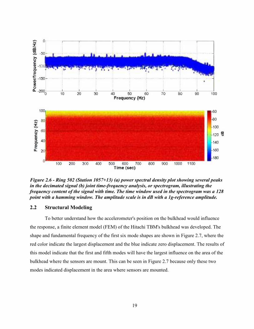
Figure 2.6 - Ring 502 (Station 1057+13) (a) power spectral density plot showing several

peaks in the decimated signal (b) joint time-frequency analysis, or spectrogram,

illustrating the frequency content of the signal with time. The time window used

in the spectrogram was a 128 point with a hamming window. The amplitude

scale is in dB with a 1g-reference amplitude. .............................................................19

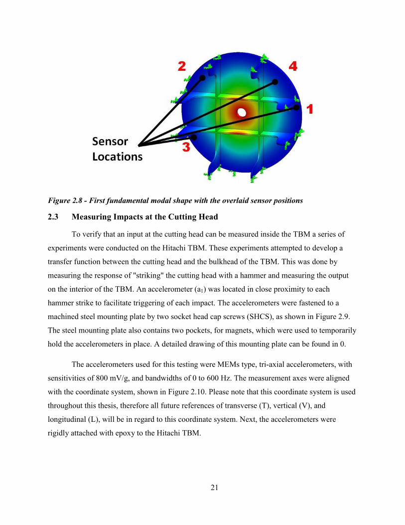
Figure 2.7 - Modal analysis of the bulkhead showing the first six fundamental mode shapes .....20

Figure 2.8 - First fundamental modal shape with the overlaid sensor positions............................21

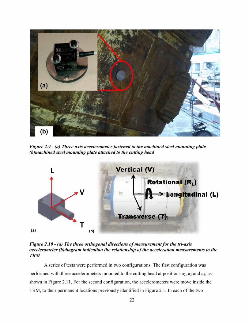
Figure 2.9 - (a) Three axis accelerometer fastened to the machined steel mounting plate

(b)machined steel mounting plate attached to the cutting head ..................................22

Figure 2.10 - (a) The three orthogonal directions of measurement for the tri-axis

accelerometer (b)diagram indication the relationship of the acceleration

measurements to the TBM ..........................................................................................22

Figure 2.11 - Tap test map of the Hitachi TBM. The red numbered locations (0-7) are the tap

locations on the cutting head and the green numbered locations (a2, a3, a4) are the

fixed accelerometers, also located on the cutting head. ..............................................23

Figure 2.12 - Five Sequential Taps on the Cutting head at location 7. (a) shows the triggered

data from accelerometer a1L, mounted on the cutting head and measuring in the

longitudinal direction and (b) the response of accelerometer a4L, mounted on

the bulkhead and measuring in the longitudinal direction. .........................................25

Figure 2.13 - Stacked tap traces of accelerometer a2L and a zoomed section showing that the

responses for each sequential, stacked trace was consistent in time, shape and

amplitude. ...................................................................................................................26

Figure 2.14 - Frequency spectrum created by striking position 4 on the cutting head where (a)

shows the FFT of the accelerometer a1L mounted to the cutting head and (b)

shows the FFTs of the accelerometers a2L, a3L, and a4L mounted to the bulkhead

of the TBM. The amplitude scale is in dB with a 1g-reference amplitude. ................27

Figure 2.15 - Transfer function estimates for striking position 4, in the longitudinal direction,

on the TBM's cutting head. (a) Shows the response of accelerometers a2, a3 and

a4 in the transverse direction. (b) Shows the response of accelerometers a2, a3 and

a4 in the vertical direction. (c) Shows the response of accelerometers a2, a3 and a4

in the longitudinal direction. .......................................................................................28

ix

Figure 2.16 - Comparison of two sets of transfer function estimates, where (a)-(c) are the

response of striking the cutting head at position 2 in the T,V, and L directions,

respectively. (d)-(f) are the results of striking the cutting head at position 6 in the

T,V, and L directions, respectively. The amplitude scale is in dB with a 1g-

reference amplitude. ...................................................................................................29

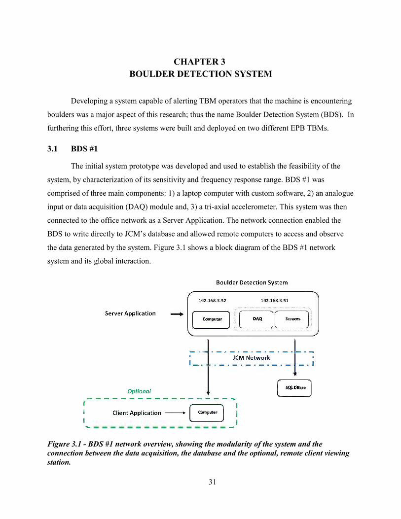
Figure 3.1 - BDS #1 network overview, showing the modularity of the system and the

connection between the data acquisition, the database and the optional, remote

client viewing station. .................................................................................................31

Figure 3.2 - Cross section of the Hitachi TBM indicating the location of BDS #1 and

showing the main thrust bearing detail .......................................................................32

Figure 3.3 - Screen shot of BDS #1 operator's screen ...................................................................33

Figure 3.4 - TBM Coordinate System............................................................................................34

Figure 3.5 - (a) Example data set from the a1V accelerometer of BDS #1(b) zoomed section,

illustrating under sampled data ...................................................................................35

Figure 3.6 - BDS #2, containing an industrial power supply, a real-time NI CompactRIO

embedded controller and 16 bit analog input card ......................................................36

Figure 3.7 - (a) Cross section of the Hitachi TBM showing the location of the four

accelerometers (b) the measurement coordinate system as it relates to the TBM ......36

Figure 3.8 - Location of the two accelerometers at the TYSSE project, which was the second

field site. Courtesy of Caterpillar Inc. ........................................................................37

Figure 3.9 - (a) Twenty minute sample of operational data and (b)vibration data for sensor a1

in the transverse (T), vertical (V) and longitudinal (L) directions overlaid with

their respective RMS signals. .....................................................................................38

Figure 3.10 - Comparison (a) diagram of cutting head spokes interacting with a boulder (b)

simulated impact signature of the boulder striking a spoke approximately every 9

sec. ..............................................................................................................................39

Figure 3.11 - simplified cutting head model illustrating three different acceleration frequency

responses (c) due to tooth geometry (a) and tooth-geological interaction scenarios

(b). ...............................................................................................................................40

x

Figure 3.12 - Time domain acceleration data after combining and zero padding files to

produce a near continuous ring segment data set for the sensor a1L taken

excavation of Ring 502 (Station 1057+13) at field site #1. ........................................41

Figure 3.13 - (a) sensor a3L acceleration time histories during the 20 minute excavation of

Ring 502 (Station 1057+13) (b) highlights peak values above a threshold of 0.25

g. .................................................................................................................................42

Figure 3.14 - (a) Power spectral density of Ring 502 (Station 1057+13) (b) Joint time-

frequency spectrogram. The amplitude scale is in dB with a 1g reference

amplitude. ...................................................................................................................43

Figure 3.15 - Dividing the vibration data into successive revolutions and spokes. .......................44

Figure 3.16 - 46 stacked revolutions of accelerometer a4L data during Ring 502 .........................45


sensor a1 in the transverse (T), vertical (V) and longitudinal (L) directions

overlaid with their respective RMS signals. ...............................................................46

Figure 3.18 - Approximate location of TBM during Ring 684 (Station 1048+04), showing the

TBM's proximity to the CDF and existing construction of Interstate 5. ....................47

Figure 3.19 - (a) The stacked a1L accelerometer data showing revolutions 73:97 for Ring 684

(Station 1048+04) (b) zoomed section showing spikes in revolution 84 and 90,

respectively. ................................................................................................................47

Figure 3.20 - (a) Operational Data (OP) of Ring 684 (Station 1048+04) (b) joint time-

frequency spectrogram of a1T where the period between 15-28 seconds is the

cutting head changing directions and the sloping line (22-28 second range) is the

cuttinghead increase in RPM and the spike at 123 seconds. The amplitude scale

is in dB with a 1g reference amplitude. ......................................................................48

Figure 3.21 - (a) Several spikes found in the 76th revolution of the excavation of Ring 684

(Station 1048+04) (b) zoomed section identifying three spikes. ................................49

Figure 3.22 - (a) Operational data (OP) and (b) sensor 1 acceleration time histories during the

excavation of Ring 601 (Station 1052+19). ................................................................50

Figure 3.23 - Vibration data from Ring 601 (Station 1052+19) accelerometer a1L, where (a)

is revolution #1 (b) is revolution #2, and (c) is the cross correlation between

revolution 1 &2. ..........................................................................................................51

xi

Figure 3.24 - Vibration data from Ring 601 (Station 1052+19) accelerometer a1L, where (a)

is revolution #4 (b) is revolution #5, and (c) is the cross correlation between

revolution 4 &5. ..........................................................................................................51

Figure 3.25 - (a) The stacked revolution data of accelerometer a3L for Ring 601 for

revolutions 4 and 5 (b) zoomed section showing the nearly perfect correlation

between successive revolutions. .................................................................................52

Figure 4.1 - Vibration data from Ring 502 (Station 1057+13) for sensor a1 in the transverse

(T), vertical (V) and longitudinal (L) directions overlaid with their respective

RMS signals ................................................................................................................55

Figure 4.2 - Vibration levels at the beginning of Ring 502 (Station 1057+13) and at the end

of Ring 507 (Station 1056+88). (a) shows the vertical acceleration starting to rise

as the cutting head begins to rotate and contacts the face, then fall as the

excavation is complete. (b) shows a spectrogram of the vertical acceleration

where the sloping line (2-10 second range) illuminates the increase in RPM and

then the opposite (56-59 second range) as the cutting head comes to a stop. In (b)

the scale is in dB with a 1g reference. ........................................................................55

Figure 4.3 - (a) SV of the longitudinal accelerometers for Ring 502 (Station 1057+08), (b)

SV of the longitudinal accelerometers for Ring 507 (Station 1056+88) ....................57

Figure 4.4 - (a) SV of the longitudinal accelerometers for Ring 358 (Station 1064+32), (b)

SV of the longitudinal accelerometers for Ring 502 (Station 1057+08) ....................58

Figure 4.5 - (a) Plot of the fundamental frequency vs. rotation rate for the four

accelerometers in the Transverse direction. (b) Plot of the fundamental frequency

vs. rotation rate for the four accelerometers in the vertical direction. (c) Plot of

the fundamental frequency vs. rotation rate for the four accelerometers in the

longitudinal direction. .................................................................................................58

Figure 4.6 - Linear fit of the fundamental frequency vs. rotation rate for the accelerometers in

the longitudinal direction. ...........................................................................................59

Figure 4.7 - Singular Value Decomposition (SVD) on the fundamental frequencies vs.

rotational rate. .............................................................................................................60

Figure 4.8 - Plot of the top three SV frequencies vs. rotation rate, illustrating a strong linear

dependence on rotation rate. .......................................................................................61

xii

Figure 4.9 - Plot showing the fundamental frequencies of the four longitudinal

accelerometers normalized by rotation rate. ...............................................................62

Figure 4.10 - Plot showing the top three SV frequencies of the longitudinal accelerometers

normalized by rotation rate. ........................................................................................62

Figure 5.1 - Geological conditions along the U230 tunnel project [14] ........................................65

Figure 5.2 - (a) Operational Data (OP) and (b) sensor 1 acceleration time histories (full

waveform and RMS amplitude) during excavation of Ring 502 (Station

1057+13). ....................................................................................................................67

Figure 5.3 - Full waveform records and histograms of a1 vibration for ring 502 (Station

1057+13) showing the stochastic nature of the captured acceleration signals and

the oscillatory nature of the RMS response influenced by cutting head position. .....68

Figure 5.4 - Bulkhead vibration at the beginning of Ring 502 excavation (Station 1057+13)

and at the end of Ring 507 excavation (Station 1056+88). (a) a1V time history as

the cutting head begins to rotate and contacts the face and as the excavation is

completed. (b) Joint time-frequency spectrogram of a1V where the sloping line

(2-10 second range) illuminates the increase in RPM and then the opposite (56-

59 second range) as the cutting head comes to a stop. The amplitude scale is in

dB with a 1g reference amplitude. ..............................................................................69

Figure 5.5 - (a) Operational Data (OP) and (b) sensor 1 acceleration time histories during the

74 minute excavation of Ring 679 (Station 1048+29). See Figure 1 for L, T and

V directions. ................................................................................................................70



V directions. ................................................................................................................72



V directions. ................................................................................................................72



V directions. ................................................................................................................73

xiii

Figure 5.9 - (a) time history data from accelerometer a1L during the 29 minute excavation of

Ring 698 (Station 1047+33). (b) zoomed section showing multiple captured

spikes. .........................................................................................................................74

Figure 5.10 - RMS vibration values and operating data during the 2nd half of the South

bound tunnel (a) shows the Advance Rate, Torque, Rotational Rate and EPB

Pressure (b) shows the geological profile (c) shows the RMS values of the a1

accelerometer in the three principle directions, T,V,L and the Standard Deviation

of the measurement at seven boring locations (d) shows the ratios between

a1LRMS / a1VRMS and a1LRMS / a1TRMS. ........................................................................76

Figure 5.11 - Comparison of Specific Energy with RMS vibration in the a1V direction. .............78

Figure 6.1 - Rigid body directions and their relationship to the TBM ..........................................81

Figure 6.2 - Graphical illustration showing how the transverse (axT) and vertical (axV)

accelerometer measurements are combined to for the rotational acceleration

(aRLx) ...........................................................................................................................82

Figure 6.3 - (a) Simulated Sensor positions, where each sensor is rotated by 90 degree and

the same distance from the center of the bulkhead (b) Sensor coordinate system

shown as it relates to the TBM. ..................................................................................84

Figure 6.4 - Simulated sensor values and directions to produce a torque around the

longitudinal axis. .........................................................................................................84

Figure 6.5 - Simulated data showing the effects of the PM filtering on data that produces a

rotational acceleration around the longitudinal axis. ..................................................85

Figure 6.6 - Simulated data show the effects of the principal motion filtering on data that

produces a torque around the longitudinal axis. 5% noise has been add to the

amplitude and 0.1% noise has been added to the phase of each signal. .....................86


produces a torque around the longitudinal axis. 5% noise has been add to the

amplitude and 0.1% noise has been added to the phase of each signal and the

principal motion results have been averaged. .............................................................87

Figure 6.8 - Sensor locations and the coordinate system used to describe the sensor outputs ......88

Figure 6.9 - Results of the principal motion calculations, showing accelerations that produce

a net torque value will result in rigid body motion .....................................................88

xiv

Figure 6.10 - (a) Operational data (OP) of 684 (Station 1048+04) (b) joint time-frequency

spectrogram of a1T where the period between 15-28 seconds is the cutting head

changing directions and the sloping line (22-28 second range) is the cutting head

increase in RPM and the spikes at 122 seconds and 130 seconds are the events in

question. The amplitude scale is in dB with a 1g reference amplitude. .....................89

Figure 6.11 - (a) Spikes in Ring 684 (Station 1048+04) (b) zoomed section showing the

oscillations of the largest peak shown in (a) for the a1T, a1V and a1L directions. .....90

Figure 6.12 - Results of the principal motion calculations for the big spike of Ring 684 .............91


oscillations of a peak near the 25 minute mark (a) for the a1T, a1V and a1L

directions. ....................................................................................................................91

Figure 6.14 - Results of the principal motion calculations for the spike of Ring 685near the

25 minute mark. ..........................................................................................................92

Figure 7.1 - Histogram of the percent of papers that had an academic contributor, where the

data was collected from the North American Tunneling Conference (NAT) for

the year: 2002, 2004, 2006, 2008, 2010, 2012 and from the Rapid Excavation and

Tunneling Conference (RETC) for the year: 2001, 2003, 2005, 2007, 2009,

2011,2013 ...................................................................................................................98

Figure A-1 - Steel mounting plate for accelerometers. ................................................................115

Figure B-1 - Estimate of DAQ noise floor (a) FFT of the accelerometer mounted to the

cutting head (b) FFT of the accelerometers mounted to the bulkhead of the TBM.

The amplitude scale is in dB with a 1g-reference amplitude. ...................................116

Figure C-1 - Transfer function estimates for striking position 0 on the TBM's cutting head.

(a) Shows the response of accelerometers a2, a3 and a4 in the transverse direction.

(b) Shows the response of accelerometers a2, a3 and a4 in the vertical direction.

(c) Shows the response of accelerometers a2, a3 and a4 in the longitudinal

direction. The amplitude scale is in dB with a 1g-reference amplitude. ..................117




xv































xvi



Figure D-1 - Calibration for transverse axis 1 .............................................................................125

Figure D-2 - Calibration for transverse axis 2 .............................................................................125

Figure D-3 - Calibration for longitudinal axis .............................................................................126

Figure D-4 - Calibration for the vertical axis...............................................................................126

Figure F-1 - (a) TBM operational data vs. station (b) RMS vibration data vs. station in the

a1T, a1V and a1L directions. ......................................................................................129

Figure F-2 - Results of SOM cluster nearest neighbor distances with (a) a 4x4 topology, (b) a

8x8 topology, (c) a 16x16topology , and (d) a 32x32 topology. ..............................131

Figure F-3 - Results of the neuron weights for each of the eighteen inputs, where each input

is shown in (a) a 4x4 topology, (b) a 8x8 topology, (c) a 16x16topology , and (d)

a 32x32 topology. .....................................................................................................132

Figure F-4 - Results of the relative number of data points affiliated with each neuron for (a) a

4x4 topology, (b) a 8x8 topology, (c) a 16x16topology , and (d) a 32x32

topology. ...................................................................................................................133

Figure F-5 - Spatial representation of the neuron's weight positions for (a) the Seattle OP and

vibration data, and (b) an example data set. .............................................................134

Figure F-6 - Boring locations and class designations indicated on the cross section of the

University Link project in Seattle, WA. ...................................................................135

Figure F-7 - Graphical program used to train, validate and develop the decision tree. ...............136

Figure F-8 - Graphic representation of a decision tree, where each leaf (shown in red)

indicates the codification of the data set. ..................................................................137

Figure F-9 - Graphic representation of the decision tree obtained from using KNIME to

identify the correlations between OP and vibration data and soil type. ...................138


identify the correlations between OP and soil type. .................................................138


identify the correlations between vibration and soil type. ........................................139

Figure F-12 - Results of the ten class decision tree obtained by applying the algorithm to the

entire set of data. .......................................................................................................140

xvii

LIST OF TABLES

Table 1 - Gear Operational Frequencies for the Hitachi TBM ......................................................13

Table 2 - Bearing Operational Frequencies for the Hitachi TBM .................................................16

Table 3 - Ring 502, Expected Gear and Bearing Operating Frequencies at 2.2 RPM ...................17

Table 4 - Tap Test Descriptions .....................................................................................................23

Table 5 - Error Analysis of Linear Correlation ..............................................................................60

Table 6 - Parameters used for unsupervised learning ..................................................................130

Table 7 - Summary of Decision Tree Results ..............................................................................140

Table 8 - UC&T Schools .............................................................................................................142

xviii

ACKNOWLEDGMENTS

There have been a number of people who have supported me through this process and

have made this journey possible. First, I would like to thank all of the wonderful people in the

SmartGeo program; their friendship, insight, and even commiseration have made such a fantastic

but grueling program truly memorable. Second, I would like to thank my advisors and committee

members for their ideas and willingness to guide me through the PhD machine. Next, I would

like to thank my friends and family for their support. Finally, I would like to thank my wife,

Christina, and our three amazing children, Katy, Anna, and Clara, for their sacrifices,

inspirations, and commitment in seeing me through this growth. I could not have done it without

you!

1

CHAPTER 1

INTRODUCTION

While Tunnel Boring Machines (TBMs) are robust, multimillion-dollar machines, their

performance is directly related to their uptime and the reliability. A significant portion of this

capability can be attributed to the operator’s ability to modify the TBM's operating parameter in

response to environmental changes. Currently there are few mechanisms available to inform the

operator of such environmental changes. One such example is encountering boulders in the

tunnel alignment. While this occurrence is often anticipated, the precise location cannot be

predicted and therefore the operator cannot modify the machine's operation to prevent damage. If

a methodology were developed to both detect and inform the operator of changing geological

conditions, such as boulder(s), the machine's life would be extended and costly downtime could

be avoided.

While the goal of this research is to investigate whether a passive, vibration based

system, can provide information about ground condition, including boulders, in the soft ground

tunneling environment, there are a number of fundamental research questions that need to be

addressed and are guiding this research.

What is the change in vibratory response of a TBM to non-stationary or time-varying

operational parameters, such as torque, rpm, thrust, pressure, etc?

Does interaction with geologic features produce measurable changes in TBM vibration?

o Can these changes be explained, rationalized, characterized?

What is the best way to measure the change of a TBM's vibratory response to time-

varying parameters, geology and environmental conditions?

o Can these vibrational changes be explained?

o Can these vibrational changes be modeled?

These fundamental questions are addressed by developing a framework that enables

collecting experimental vibration-results from operating TBMs. In this framework the

experimental results have been combined with the machine's operational data (torque, rpm,

thrust, pressure, etc.) to develop a global understanding of how geological changes influence the

machine's operation.

2

1.1 EPB TBMs

There are two major categories of TBMs, hard rock and soft ground[1]. This research

targets the soft ground category, where there are generally three types of TBMs: 1) slurry shield

(SS), 2) earth pressure balance (EPB), and 3) open face machines. This research focuses on the

EPB TBMs. A cross-section of a typical EPB TBM can be seen in Figure 1.1.

Figure 1.1 - Cross section of the Hitachi EPB TBM, showing the location of key components.

This machine was used in Seattle, Washington on the University Link Light Rail Extension as

part of the U230 contract.

EPB TBMs consist primarily of a cutting head to pulverize incident material, a conveyor

to remove the material, and locomotion system to facilitate tunneling. The primary difference

between an EPB machine and a hard rock machine is the EPB machine's ability to support the

excavation face by providing a supporting pressure. This supporting pressure is accomplished by

using the machine to create a seal between the excavated tunnel, which is at atmospheric

pressure, and the excavation face, which is typically above atmospheric pressure. Figure 1.2

shows a diagram of this pressure balance.

3

Figure 1.2 - Diagram of the earth pressure vs. machine pressure in EPB tunneling, where the

blue and brown pressure gradients represent the soil and hydraulic heads respectively and the

red is the machine generated support pressure or Earth Pressure Balance (EPB).

Over the past 20 years EPB machines have become more commonly used in the tunneling

industry. This increased use is a result of tunneling jobs becoming more prevalent in soil types

that are better suited for an EPB type machine. With this increase in use, the industry has

identified limitations of modern EPB machines. One drawback is that the seal an EPB machine

creates between the machine and the excavation makes accessing and inspecting the cutting head

and teeth difficult. Because of this difficulty, there is a need to better understand the interaction

between the machine and the soil being excavated. Ultimately this understanding could provide

insight into the machine's performance and maintenance needs without requiring personnel to

enter the pressurized face for inspections. One approach to gaining an understanding of this

interaction is measuring the TBM's vibrational response during operation.

1.2 Field Sites

Within the scope of this research is developing an understanding of a TBM and how it

operates. An overview of TBMs general practices and operations can be found in Mechanised

Shield Tunnelling [1]. Hands-on and in-depth knowledge about TBMs and the logistics of

4

tunneling projects were gained through an internship with Jay Dee Contractors, Inc., the primary

contractor working on the University Link Extension (U-Link) in downtown Seattle,

Washington. This internship took place during the summer of 2012.

This research spanned two field sites, one in Seattle, Washington and the second in

Toronto, Ontario, Canada. At each site, an EPB TBMs was instrumented with accelerometers to

passively measure vibration levels during tunneling. Slightly different experimental set-ups were

required at each site since the sites and machines were unique. Further, data collection and

experimentation were conducted at different times and tests were performed progressively to

answer the research question posed. Both field sites used precast concrete segmental linings,

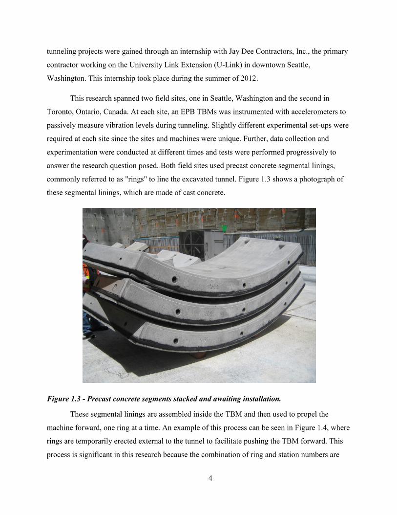
commonly referred to as "rings" to line the excavated tunnel. Figure 1.3 shows a photograph of

these segmental linings, which are made of cast concrete.

Figure 1.3 - Precast concrete segments stacked and awaiting installation.

These segmental linings are assembled inside the TBM and then used to propel the

machine forward, one ring at a time. An example of this process can be seen in Figure 1.4, where

rings are temporarily erected external to the tunnel to facilitate pushing the TBM forward. This

process is significant in this research because the combination of ring and station numbers are

5

used to delineate data sets and mark the forward progress of the machine. Each ring is 1.5 m (5

ft) in length and the station numbers are in hundreds of feet, plus tens of feet. For example, a data

set labeled Ring 502 (Station 1057 + 13), would signify the 502nd

ring with a linear position of

105713 ft. This notation is used throughout this thesis.

Figure 1.4 - Series of photographs illustrating how the TBM is propelled forward by pushing

the machine off the precast concrete segments.

1.2.1 Field Site #1

Research for the first field site took place during 2011-2012 operations on the University

Link Light Rail Tunnel project (U230) in Seattle, Washington (from the Capitol Hill Station to

Pine Street Stub Tunnel). A plan view of the alignment can be seen in Figure 1.5. The U230

project involved the mechanical excavation of twin tunnels over a distance of approximately 1

km through complex soft ground geology.

6

Figure 1.5 - Plan view of the University Link Light Rail Tunnel project (U230) alignment

This project was part of a joint venture between Jay Dee Contractors, Collucio

Construction and Michaels Corporation and is commonly referred to as JCM U-link Joint

Venture or more commonly JCM. Figure 1.6 shows a photograph of the machine and trailing

gear prior to launch.

7

Figure 1.6 - JCM's 6.44 m diameter Hitachi EPB TBM nearing completion of its assembly as

part of the University Link Light Rail Extension (U230) in Seattle, Washington

1.2.2 Field Site #2

The second TBM was located in Toronto, Canada and was part of the Toronto-York

Spadina Subway Extension (TYSSE). This TBM was being operated by a joint venture between

McNally, Kiewit and Aecon, referred to as the MKA partnership. An image of the TBM for this

project and a plan view of the proposed tunnel are shown in Figure 1.7 and Figure 1.8,

respectively.

1.3 Previous Work

To investigate the posed research questions, a literature review was performed. The

results of this survey have revealed that correlating TBM vibration to geology is a novel idea.

There is, however, a study by Teale [2], that related the specific energy of rock drilling with the

crushing strength of rock. This work was extended by Celada et al [3], to explore the correlation

8

between the calculated specific energy generated by a TBM and the properties of the excavated

rock. Both studies were performed in rock and therefore only offer a suggested approach to

follow in the characterization of mixed soil.

Figure 1.7 - 6.2 m diameter Caterpillar EPM TBM being re-assembled for its second launch

on the TYSSE project

Figure 1.8 - Plan view of the York University alignment

9

Additionally, there have been several studies that have investigated the use of vibration-

based measurements for the diagnostics of problems in downhole drilling. Cooper et al [4]

showed that the vibration generated by tricone drill bits could be used to diagnose worn bits or

failed bearings. Further work by Heisig et al [5] showed that downhole vibration measurements

could extend measurement-while-drilling (MWD) based services to include the identification of

stick-slip, whirl and bit bounce, three vibration-related complications. Recently, improved

diagnostic capabilities have been achieved by embedding sensors in or near the cutting tools.

These results by Hoffman et al [6] have shown that embedded sensors can accurately measure

"downhole dysfunctions" and assist in optimizing the drilling process. While none of these works

focused on TBMs or the specific relationship between vibration and geology, they do offer

insight as to the future prospects of harvesting information from passive vibration measurements.

Alternatively, much of the analysis and results presented in this thesis have leveraged

previous works in vibration analysis and signal processing. Specifically, the work of Ewins in

experimental modal analysis [7], the work by Brincker et al in operational modal analysis [8],

and the work of Bendat et al, in signal processing [9]. More detail on these subjects and their use

will follow in the body of this document, however the contributions of these authors are

graciously acknowledged.

1.4 Outline and Contributions

In this dissertation, the complex interaction between TBMs and the excavated soil is

investigated through TBM measurements. The following gives an outline of this thesis by

chapter and briefly summarizes the contributions.

In Chapter 2 an overview of the expected vibration sources of a TBM are explored. These

sources include electro-mechanical components, as well as the structural response of the location

in which the sensors are mounted. Next, the estimates are compared with collected field data and

similarities are discussed. Additionally, the measured bulkhead responses, of events generated at

the cutting head, are evaluated.

In Chapter 3 the evolution of the Boulder Detection System (BDS) is developed. This

includes a hypothesis for what the system is expected to measure, system upgrades as the

research progressed, and an overview of both the passive vibration measurements and the

10

operating data collected by the TBM. Next, these two data sources are combined and used to

explore methods for detecting boulders.

In Chapter 4 an experimental vibration technique, referred to as operational modal

analysis (OMA), was explored to characterize the TBM. The goals of this technique is to

investigate the feasibility of experimentally characterizing the TBM’s response.

In Chapter 5, the body of a journal paper submitted to Tunneling and Underground Space

Technology (TUST), is presented. This paper explores the combination of the passive vibration

data, the TBM operational data, and geological information to correlate changes in geology.

In Chapter 6, a filtering process called Principal Motion (PM) is explored. This approach

provides a mechanism for separating the flexible motion from the rigid body motion in a grouped

set of measurements. For this research, a combination of theoretical modeling and experimental

measurements are evaluated to investigate the detection of rigid body motion.

In Chapter 7, a non-technical investigation into the relationship between academia and

industry in the underground construction and tunneling (UC&T) field is explored. This chapter

fulfills the SmartGeo requirement of integrating a social or political aspect of one's technical

research to gain a more holistic perspective. The goal of this work is to investigate the barriers

and opportunities that drive potential collaboration between academia and industry in the UC&T

field.

11

CHAPTER 2

CHARACTERIZING THE VIBRATION OF A TBM

A TBM has many structural components that exhibit vibrational responses during day-to-

day operations. Many of these responses are the result of the excitation produced from active

components, such as motors and actuators, and others might be from the machine's interaction

with the geology. To establish a foundation, prior to investigating the geologically inducted

vibration, this section will characterize the vibrational responses due to active components.

2.1 TBM Component Operating Frequencies

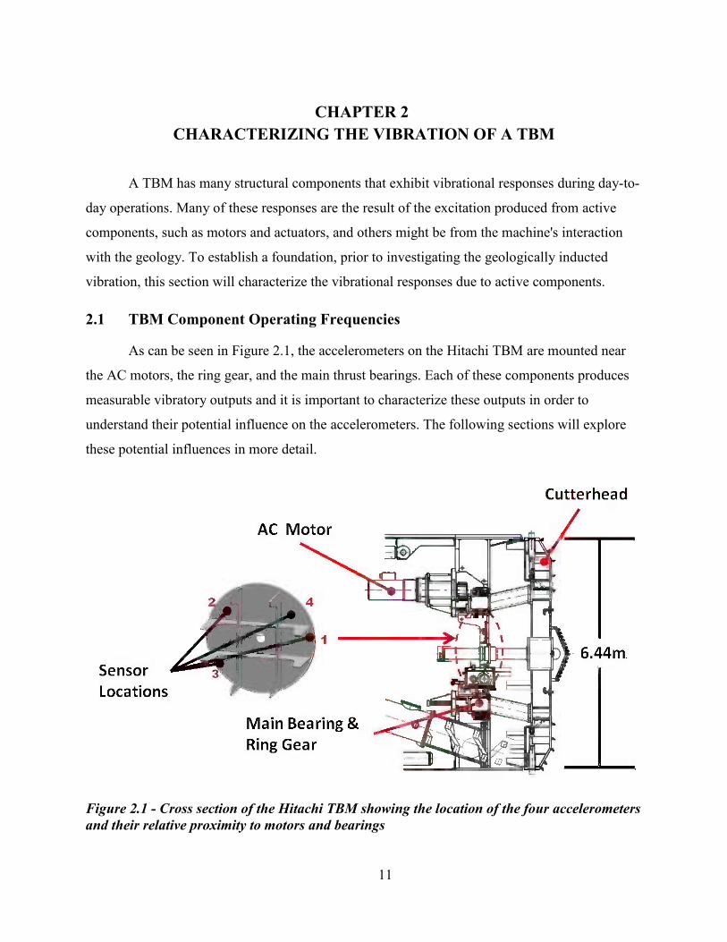
As can be seen in Figure 2.1, the accelerometers on the Hitachi TBM are mounted near

the AC motors, the ring gear, and the main thrust bearings. Each of these components produces

measurable vibratory outputs and it is important to characterize these outputs in order to

understand their potential influence on the accelerometers. The following sections will explore

these potential influences in more detail.

Figure 2.1 - Cross section of the Hitachi TBM showing the location of the four accelerometers

and their relative proximity to motors and bearings

12

2.1.1 Gear Induced Vibration

To investigate whether or not there was an influence in the collected data due to the

motors, and their gear trains, a series of analyses were performed to quantify the frequency

spectrum due to these components. The cutting head of the Hitachi TBM, at site #1, is driven by

eight AC. These motors are coupled in two stages of reduction. The first is a planetary gearbox

and the second is a ring and pinion arrangements. A simplified schematic of the drive train and

the gear ratios are shown in Figure 2.2.

Figure 2.2 - Hitachi TBM Drive Train Schematic

From this schematic and the equations found in [10] a set of equations are developed that

describe the expected gear meshing frequencies and their subsequent harmonics [11].

(2.1)

The first frequency of interest is the gear meshing frequency, which is the frequency at

which the set of two gears mesh together. This frequency can be calculated using Equation (2.2).

(2.2)

13

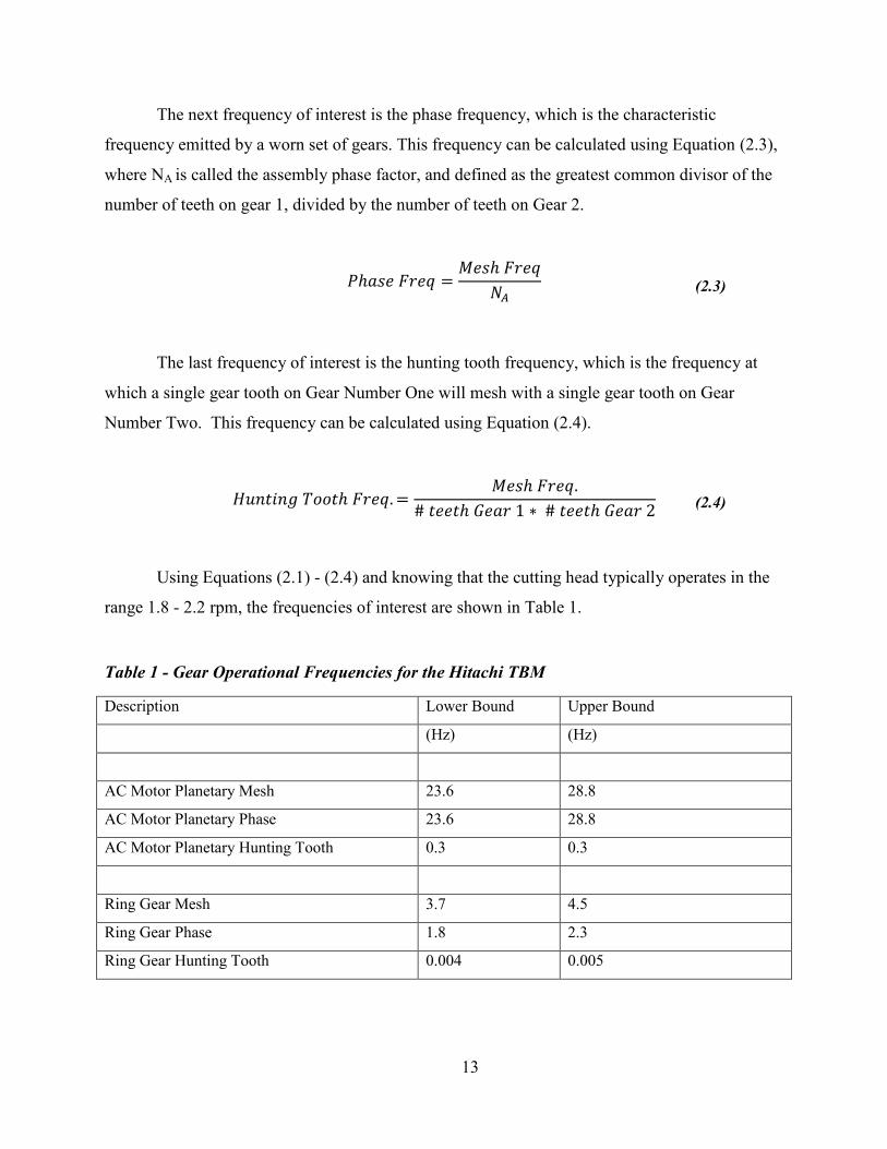
The next frequency of interest is the phase frequency, which is the characteristic

frequency emitted by a worn set of gears. This frequency can be calculated using Equation (2.3),

where NA is called the assembly phase factor, and defined as the greatest common divisor of the

number of teeth on gear 1, divided by the number of teeth on Gear 2.

(2.3)

The last frequency of interest is the hunting tooth frequency, which is the frequency at

which a single gear tooth on Gear Number One will mesh with a single gear tooth on Gear

Number Two. This frequency can be calculated using Equation (2.4).

(2.4)

Using Equations (2.1) - (2.4) and knowing that the cutting head typically operates in the

range 1.8 - 2.2 rpm, the frequencies of interest are shown in Table 1.

Table 1 - Gear Operational Frequencies for the Hitachi TBM

Description Lower Bound Upper Bound

(Hz) (Hz)

AC Motor Planetary Mesh 23.6 28.8

AC Motor Planetary Phase 23.6 28.8

AC Motor Planetary Hunting Tooth 0.3 0.3

Ring Gear Mesh 3.7 4.5

Ring Gear Phase 1.8 2.3

Ring Gear Hunting Tooth 0.004 0.005

14

2.1.2 Bearing Induced Vibration

The bearing layout and arrangement was estimated from Figure 2.3, where the diameter

of the main thrust bearing, Dball = 80 mm and the distance of the main thrust bearing to the center

of the machine, Dpitch = 2748 mm.

Figure 2.3 - Hitachi main thrust bearing Schematic, showing the dimensions for Dball = 80

mm and Dpitch = 2748 mm

There are a number of important gear related frequencies. In the equations that follow, fs

is the rotational frequency of the shaft in revolutions per second.

The fundamental train frequency:

(2.5)

, the contact angle between the bearing and the race

Ball spin frequency:

15

(2.6)

Outer race frequency:

(2.7)

Inner race frequency:

(2.8)

N = the number of rollers or balls.

Fundamental train order:

(2.9)

Ball spin order:

(2.10)

These equations are taken from National Instrument's help files from the Sound and

Vibration Measurement Suite[10]. In the next section, examples of this analysis will be explored

using data taken during the Seattle U230 project.

2.1.3 Example Gear and Bearing Operation Frequencies from the Seattle Project

Using the above calculations and data from Ring 502 (Station 1057+13) shown in Figure

2.4, a frequency analysis was performed. Figure 2.4(a) presents the TBM's operational

parameters (OP), which are the cutting head's rate of rotation (N), the advance rate (AR), the

torque (T), the thrust force (F), and the face pressure (σ).

16

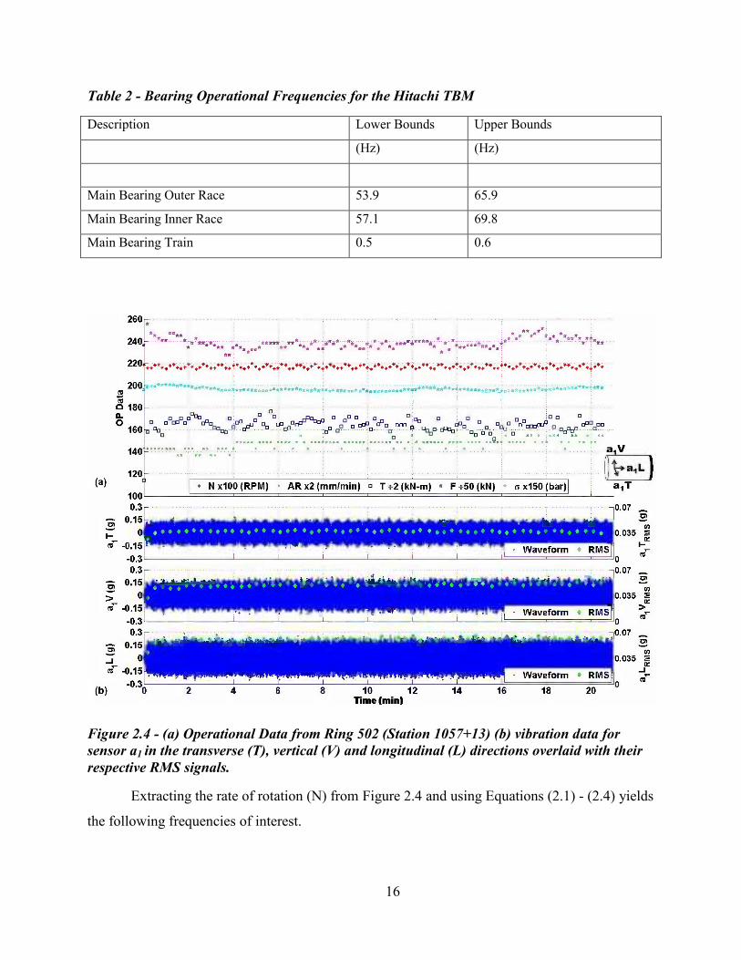
Table 2 - Bearing Operational Frequencies for the Hitachi TBM

Description Lower Bounds Upper Bounds

(Hz) (Hz)

Main Bearing Outer Race 53.9 65.9

Main Bearing Inner Race 57.1 69.8

Main Bearing Train 0.5 0.6


sensor a1 in the transverse (T), vertical (V) and longitudinal (L) directions overlaid with their

respective RMS signals.

Extracting the rate of rotation (N) from Figure 2.4 and using Equations (2.1) - (2.4) yields

the following frequencies of interest.

17

Table 3 - Ring 502, Expected Gear and Bearing Operating Frequencies at 2.2 RPM

Description Frequency

(Hz)

AC Motor Planetary Mesh 28.8

AC Motor Planetary Phase 28.8

AC Motor Planetary Hunting Tooth 0.3

Ring Gear Mesh 4.5

Ring Gear Phase 2.3

Ring Gear Hunting Tooth 0.005

Main Bearing Outer Race 65.9

Main Bearing Inner Race 69.8

Main Bearing Train 0.6

Since the vibration data appears to be random in nature, the appropriate method for

estimating the frequency spectrum, as discussed by Bendat et al [9], is to use the power spectral

density (PSD) calculation. Then calculating PSD of the recorded accelerometer record, the

frequency content of the signal can be compared to the expected values shown in Table 3. The

PSD is the Fourier transform of the auto correlation, and is calculated by applying Equations

(2.11) and (2.12) sequentially.

(2.11)

(2.12)

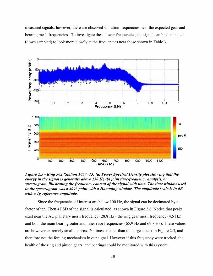
As can be seen in Figure 2.5 the majority of the energy is well above the tabulated values,

therefore the presented gear and bearing frequencies are not the driving mechanism in our

18

measured signals; however, there are observed vibration frequencies near the expected gear and

bearing mesh frequencies. To investigate these lower frequencies, the signal can be decimated

(down sampled) to look more closely at the frequencies near those shown in Table 3.

Figure 2.5 - Ring 502 (Station 1057+13) (a) Power Spectral Density plot showing that the

energy in the signal is generally above 150 Hz (b) joint time-frequency analysis, or

spectrogram, illustrating the frequency content of the signal with time. The time window used

in the spectrogram was a 4096 point with a Hamming window. The amplitude scale is in dB

with a 1g-reference amplitude.

Since the frequencies of interest are below 100 Hz, the signal can be decimated by a

factor of ten. Then a PSD of the signal is calculated, as shown in Figure 2.6. Notice that peaks

exist near the AC planetary mesh frequency (28.8 Hz), the ring gear mesh frequency (4.5 Hz)

and both the main bearing outer and inner race frequencies (65.9 Hz and 69.8 Hz). These values

are however extremely small, approx. 20 times smaller than the largest peak in Figure 2.5, and

therefore not the forcing mechanism in our signal. However if this frequency were tracked, the

health of the ring and pinion gears, and bearings could be monitored with this system.

19

Figure 2.6 - Ring 502 (Station 1057+13) (a) power spectral density plot showing several peaks

in the decimated signal (b) joint time-frequency analysis, or spectrogram, illustrating the

frequency content of the signal with time. The time window used in the spectrogram was a 128

point with a hamming window. The amplitude scale is in dB with a 1g-reference amplitude.

2.2 Structural Modeling

To better understand how the accelerometer's position on the bulkhead would influence

the response, a finite element model (FEM) of the Hitachi TBM's bulkhead was developed. The

shape and fundamental frequency of the first six mode shapes are shown in Figure 2.7, where the

red color indicate the largest displacement and the blue indicate zero displacement. The results of

this model indicate that the first and fifth modes will have the largest influence on the area of the

bulkhead where the sensors are mount. This can be seen in Figure 2.7 because only these two

modes indicated displacement in the area where sensors are mounted.

20

Figure 2.7 - Modal analysis of the bulkhead showing the first six fundamental mode shapes

Superimposing the sensor positions on the bulkhead, as shown in Figure 2.9, illustrates

that the sensors are located in the regions expected to have the lowest levels of displacement.

This is desirable because, ideally the sensors should measure the response of the total system and

not just the localized bulkhead response. That being said, the first mode shape's response begins

to infringe on the sensor locations and as the model shows, the bulkhead will deform in a

concave manner, similarly to the head of a drum, at a fundamental frequency of 348 Hz.

Referring back to the frequency response results shown in Figure 2.5, a significant

amount of energy is in close proximity to the fundamental frequencies, as indicated by the FEM.

These results suggest that the majority of the measured energy maybe the localized response of

the bulkhead. However, the entire system was not modeled, therefore influences of other

components could be contributing to this response.

21

Figure 2.8 - First fundamental modal shape with the overlaid sensor positions

2.3 Measuring Impacts at the Cutting Head

To verify that an input at the cutting head can be measured inside the TBM a series of

experiments were conducted on the Hitachi TBM. These experiments attempted to develop a

transfer function between the cutting head and the bulkhead of the TBM. This was done by

measuring the response of "striking" the cutting head with a hammer and measuring the output

on the interior of the TBM. An accelerometer (a1) was located in close proximity to each

hammer strike to facilitate triggering of each impact. The accelerometers were fastened to a

machined steel mounting plate by two socket head cap screws (SHCS), as shown in Figure 2.9.

The steel mounting plate also contains two pockets, for magnets, which were used to temporarily

hold the accelerometers in place. A detailed drawing of this mounting plate can be found in 0.

The accelerometers used for this testing were MEMs type, tri-axial accelerometers, with

sensitivities of 800 mV/g, and bandwidths of 0 to 600 Hz. The measurement axes were aligned

with the coordinate system, shown in Figure 2.10. Please note that this coordinate system is used

throughout this thesis, therefore all future references of transverse (T), vertical (V), and

longitudinal (L), will be in regard to this coordinate system. Next, the accelerometers were

rigidly attached with epoxy to the Hitachi TBM.

22

Figure 2.9 - (a) Three axis accelerometer fastened to the machined steel mounting plate

(b)machined steel mounting plate attached to the cutting head

Figure 2.10 - (a) The three orthogonal directions of measurement for the tri-axis

accelerometer (b)diagram indication the relationship of the acceleration measurements to the

TBM

A series of tests were performed in two configurations. The first configuration was

performed with three accelerometers mounted to the cutting head at positions a2, a3 and a4, as

shown in Figure 2.11. For the second configuration, the accelerometers were move inside the

TBM, to their permanent locations previously identified in Figure 2.1. In each of the two

23

configurations, the cutting head was struck five times in the L direction and the response was

recorded. A detailed description of the location and component of the TBM that was struck, can

be found in Table 4.

Figure 2.11 - Tap test map of the Hitachi TBM. The red numbered locations (0-7) are the tap

locations on the cutting head and the green numbered locations (a2, a3, a4) are the fixed

accelerometers, also located on the cutting head.

Table 4 - Tap Test Descriptions

The accelerometer responses were recorded at 2.5 kHz, by triggering the DAQ to record

when a threshold was exceeded on the proximity accelerometer. The threshold was set at 0.1g,

and 512 points were recorded per tap, including 10 pre-triggered. Then the three accelerometers

were moved to their permanent location inside the machine on the bulkhead. The taps were

repeated at the same locations, measuring the response of these taps at the bulkhead. Examples

of these data sets are shown in Figure 2.12, where the accelerometers were excited by tapping on

24

the cutting head at location 7. In addition, several seconds of data was also collected, during a

period of inactivity, to estimate the DAQ noise level. FFTs of the noise levels can be found in 0,

and indicate that signals above -100 dB (1g-reference amplitude) are above the noise floor of the

DAQ system.

Location Description of location, accelerometer placement and tap direction

0 Flat steel area on the cutting head

1 Over-cutter tooth

2 Scraper, accel. was mounted on the side of the scraper and the scraper was struck directly

3 Nose cone, accel. mounted on side, struck on the side perpendicular to cutting head

4 Nose cone, accel. mounted on side, struck on the nose of the nose cone, which is normal to

the cutting head

5 Pre-cutting bit

6 Scraper, accel. was mounted on the side of the scraper and the scraper was struck directly

7 Accel. was mounted on the replaceable pre-cutter box structure

The 5 impacts or "taps" from each individual location test were then overlaid. In general,

the data points were well aligned as shown in the zoomed section of Figure 2.13, where the

response of accelerometer 2, in the longitudinal direction (a2L) is shown.

The stacked traces were then averaged together to improve the signal to noise ratio before

performing a frequency analysis. As previously shown in Figure 2.7, the region where the

sensors were mounted is expected to deform in the longitudinal direction. Therefore, FFTs were

calculated for the longitudinal accelerometer measurements. As can be seen in Figure 2.14, there

are multiple peaks that exist in both the accelerometers mounted to the cutting head and those

mounted to the bulkhead. There are a number of frequency values that correlate with those

estimated by the FEM of the bulkhead, however they exist in both the cutting head FFT and the

bulkhead FFTs. This indicates that the vibration of the cutting head is being sensed at the

bulkhead and is likely masking the unique response of the bulkhead. There is however, a peak

near 525 Hz that exists only in the bulkhead FFT, show in Figure 2.14(b). This value also

corresponds with the value expected from mode 5 of the FEA model.

25

Figure 2.12 - Five Sequential Taps on the Cutting head at location 7. (a) shows the triggered

data from accelerometer a1L, mounted on the cutting head and measuring in the longitudinal

direction and (b) the response of accelerometer a4L, mounted on the bulkhead and

measuring in the longitudinal direction.

A similar frequency analysis was not conducted for the vibration data collected from the

cutting head. One reason that this analysis was not performed was that the geometry of the

cutting head was deemed too complicated for the construction of a simple FEM. Therefore,

without the results of a model, a comparison of experimental and modeled results could not be

performed. Additionally, the goal of these experiments was to investigate the propagation of

energy from the cutting head to the bulkhead. Without the model, the results from just the cutting

head offered no benefit in understanding the transfer function between the cutting head and the

bulkhead.

The transfer function between the triggering accelerometer and the accelerometer

mounted on the structure of the TBM, was estimated by dividing the FFT of the bulkhead signal

26

by the FFT of the triggering signal. The results from this transfer function can be seen in Figure

2.15, where the magnitude of the transfer is shown in the T, V and L directions. These results

show that signals initiated at the cuttinghead produce a measureable response at the bulkhead. In

addition, there are a number of peaks in the longitudinal measurements (Figure 2.15(c)) that are

consistent with the modal frequencies of the FEM.

Figure 2.13 - Stacked tap traces of accelerometer a2L and a zoomed section showing that the

responses for each sequential, stacked trace was consistent in time, shape and amplitude.

Further, a comparison between striking similar types of cutting teeth, yields dissimilar

results. For example, the signature of the response generated by striking position 2 in the

longitudinal direction (Figure 2.16(a)), and the signature of the response generated by striking

position 6 in the longitudinal direction (Figure 2.16(d)), are unique. Since the responses are not

similar, i.e. they do not have distinct peaks at the same frequencies, the response of the structure

27

was also unique. This indicates that events generated at the cutting head are not characterizable

by a single transfer function. Similar results can be seen by comparing the vertical and

longitudinal responses, also show in Figure 2.16. Additionally, this analysis was repeated for the

remaining five positions, shown in Figure 2.11. The results for these additional tap locations

produced similar finding, and can be found in 0. These results indicate that the developed

transfer functions are of limited value, because they do not offer a solution to distinctly

characterize an event.

Figure 2.14 - Frequency spectrum created by striking position 4 on the cutting head where (a)

shows the FFT of the accelerometer a1L mounted to the cutting head and (b) shows the FFTs

of the accelerometers a2L, a3L, and a4L mounted to the bulkhead of the TBM. The amplitude

scale is in dB with a 1g-reference amplitude.

28

Figure 2.15 - Transfer function estimates for striking position 4, in the longitudinal direction,

on the TBM's cutting head. (a) Shows the response of accelerometers a2, a3 and a4 in the

transverse direction. (b) Shows the response of accelerometers a2, a3 and a4 in the vertical

direction. (c) Shows the response of accelerometers a2, a3 and a4 in the longitudinal direction.

29

Figure 2.16 - Comparison of two sets of transfer function estimates, where (a)-(c) are the

response of striking the cutting head at position 2 in the T,V, and L directions, respectively.

(d)-(f) are the results of striking the cutting head at position 6 in the T,V, and L directions,

respectively. The amplitude scale is in dB with a 1g-reference amplitude.

30

2.4 Summary

Bulkhead modeling suggested that a large portion of the measured energy would exist

between 350-525 Hz, which was found to be consistent with a PSD of the measured data.

Through modeling, it was also determined that some of the dominant measured frequencies are

likely the local modal response of the bulkhead. However, the entire system was not modeled,

therefore influences of other components are not known. In addition, there are several electro-

mechanical systems in a TBM that produce vibrations. The main contributors to these vibrations

are the components associated with driving the cutting head, such as the AC motors, the gearing

reduction, and their bearings. The expected frequency response of these components was

calculated and shown to be present in the passive vibration measurements. However, the

amplitude of these signatures are an order of magnitude smaller than the largest signals.

Additionally, through a series of field measurements the transmissibility was estimated.

These field measurements showed that impacts at the cutting head could be measured in the

interior of the TBM, however the transfer functions were of limited use for the following two

reasons. First, a distinct transfer function could not be realized, making the results unclear.

Second, the influence of the signal traveling through the thrust bearing was not characterized and

might be introducing a non-linear response.

31

CHAPTER 3

BOULDER DETECTION SYSTEM

Developing a system capable of alerting TBM operators that the machine is encountering

boulders was a major aspect of this research; thus the name Boulder Detection System (BDS). In

furthering this effort, three systems were built and deployed on two different EPB TBMs.

3.1 BDS #1

The initial system prototype was developed and used to establish the feasibility of the

system, by characterization of its sensitivity and frequency response range. BDS #1 was

comprised of three main components: 1) a laptop computer with custom software, 2) an analogue

input or data acquisition (DAQ) module and, 3) a tri-axial accelerometer. This system was then

connected to the office network as a Server Application. The network connection enabled the

BDS to write directly to JCM’s database and allowed remote computers to access and observe

the data generated by the system. Figure 3.1 shows a block diagram of the BDS #1 network

system and its global interaction.

Figure 3.1 - BDS #1 network overview, showing the modularity of the system and the

connection between the data acquisition, the database and the optional, remote client viewing

station.

32

For this prototype system a single, tri-axial sensor was constructed from two dual-axis

MEMs accelerometers. The tri-axis arrangement allowed for the investigation of dominant

direction of the induced vibration. The sensors were rated at ±18g, had a 100mV/g sensitivity

and were low-pass filtered with a 1st order resistor-capacitor (RC) filter tuned to a cutoff

frequency of approximately 50 Hz. It may have been advantageous to use a sensor with higher

bandwidth, but this device was chosen primarily because it was readily available and deemed

acceptable to serve in a proof of concept. The accelerometers were mounted on the bulkhead of

the TBM, near the main bearings. This location was chosen because it is a very structurally stiff

location, and therefore, most of the vibrational energy must travel from the cutting head, through

the bearings and into this supporting member. Figure 3.2 shows a cross section of the TBM

bulkhead, the sensor’s location, and the main thrust bearing.

Figure 3.2 - Cross section of the Hitachi TBM indicating the location of BDS #1 and showing

the main thrust bearing detail

The accelerometer output was sampled through the DAQ at 200 Hz using a custom

application. This application provided a real-time graph of the current vibration levels and an

indicator that alerted the operator of vibration levels that exceeded a programmable threshold. In

addition, there were customizable fields allowing for alteration of program parameters such as

sampling rates, trigger levels and file logging. Figure 3.3 shows a screen shot of the application.

33

Figure 3.3 - Screen shot of BDS #1 operator's screen

The application also performed the following three background tasks: 1) time stamping

logged vibrational waveform data at user configurable intervals, 2) writing notification of events

exceeding thresholds to the main SQL database and, 3) hosting remote connections for remote

monitoring and maintenance

Since the sensor package was constructed from two dual axis accelerometers to make a

single tri-axis accelerometer, there was a redundant axis. This redundant axis was arbitrary

chosen to be the second transverse axis and it is present in the data stream but not being recorded

or displayed. Figure 3.4 show the orientation of the accelerometers relative to the TBM. Since

there was a significant difference in the response of each axis on each of the accelerometers, a

calibration for each of the axes was performed. The results of this calibration can be found in 0.

34

Figure 3.4 - TBM Coordinate System

The BDS #1 system was used for the entire north-bound (NB) tunnel at filed site #1. The

results from this trial established that a ±5g accelerometer would be sufficient for capturing the

vibrations present during TBM operations. However the data indicated that the system's

bandwidth should be increased to have a bandwidth greater than 50 Hz. The need for a higher

bandwidth was established from evidence of the captured vibration signatures appearing to be

near the Nyquist frequency, as can be seen in Figure 3.5. In addition, a more reliable data

collection scheme needed to be adopted for the following three reasons: 1) the system was

running on a laptop computer that was periodically turned off, 2) the data acquisition system was

network based and not on a dedicated network , therefore prone to a number of network based

faults, and 3) the system was reliant on an operator to re-start the system upon a power outage.

3.2 BDS #2

The second Boulder Detection System (BDS #2) was a significant upgrade based on

lessons learned from using and analyzing data generated by BDS #1. A real-time embedded

controller replaced the laptop and Ethernet-based DAQ. This embedded controller allowed for

higher frequency and higher resolution sampling of the accelerometer output. Fully integrated

35

tri-axis accelerometer sensors with improved sensitivity and bandwidth were used. An improved,

industrial-quality power supply was installed. Finally, more accelerometers were used to allow

for data collection from more locations on the TBM. All of these components were housed in a

self-contained durable housing. Figure 3.6 shows a photograph of BDS #2. This system replaced

BDS #1 and was installed in January 2012 at field site #1.

Figure 3.5 - (a) Example data set from the a1V accelerometer of BDS #1(b) zoomed section,

illustrating under sampled data

BDS #2 used four tri-axial accelerometers, with sensitivities of 800 mV/g, and

bandwidths of 0 to 600 Hz. Similar to BDS #1, these sensors were placed on the structurally stiff

bulkhead, on the interior of the TBM. The sensor placement locations and measurement

directions, are shown in Figure 3.7(a) and Figure 3.7(b), respectively.

36

Figure 3.6 - BDS #2, containing an industrial power supply, a real-time NI CompactRIO

embedded controller and 16 bit analog input card

Figure 3.7 - (a) Cross section of the Hitachi TBM showing the location of the four

accelerometers (b) the measurement coordinate system as it relates to the TBM

3.3 BDS # 3

The third Boulder Detection System (BDS #3) was nearly identical to BDS #2. The

accelerometers bandwidth was increased to 0-1kHz, while the sensitivity was reduces to 400

mV/g. BDS #3 was installed at field site #2 on a similar type of TBM as used with BDS #1 and

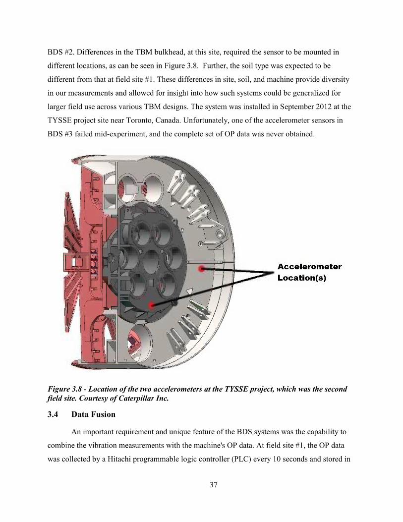
37

BDS #2. Differences in the TBM bulkhead, at this site, required the sensor to be mounted in

different locations, as can be seen in Figure 3.8. Further, the soil type was expected to be

different from that at field site #1. These differences in site, soil, and machine provide diversity

in our measurements and allowed for insight into how such systems could be generalized for

larger field use across various TBM designs. The system was installed in September 2012 at the

TYSSE project site near Toronto, Canada. Unfortunately, one of the accelerometer sensors in

BDS #3 failed mid-experiment, and the complete set of OP data was never obtained.

Figure 3.8 - Location of the two accelerometers at the TYSSE project, which was the second

field site. Courtesy of Caterpillar Inc.

3.4 Data Fusion

An important requirement and unique feature of the BDS systems was the capability to

combine the vibration measurements with the machine's OP data. At field site #1, the OP data

was collected by a Hitachi programmable logic controller (PLC) every 10 seconds and stored in

38

a Structured Query Language (SQL) database. Each data set contains a single sample of over 200

measured parameters, including quantities such as torque (T), axial thrust (F), cutting head

rotational speed (N), face pressure (), advance rate (AR), etc. The time stamp from each data

set was used to synchronize the OP data with vibration data from the BDS. Figure 3.9 shows an

example plot of results from combining some of the parameters from the two data sets. The two

data sets had vastly different sample rates. OP data was sampled at 0.1Hz while vibrational data

was taken at 2kHz: a 20,000:1 data density ratio. This vast difference in sample-rates of the two

data sets made combining them challenging.

Figure 3.9 - (a) Twenty minute sample of operational data and (b)vibration data for sensor a1

in the transverse (T), vertical (V) and longitudinal (L) directions overlaid with their respective

RMS signals.

3.5 Detecting Boulders

Collecting vibration data during operation of TBMs may elicit understanding of the

cutting head's interaction with the soil. It is hypothesized that the measured vibration correlates

with the cutting head striking fixed objects, like boulders, during excavation. For example, if a

39

TBM cutting head is rotating at a fixed rate when a boulder becomes incident on the cutting

head, we expect the vibration data to show spikes proportional to the cutting head spoke spacing

and the rotational rate of the machine. For instance, if a boulder strikes each of the six cutting

head spokes while the cutting head is rotating at 1.1RPM, as shown in Figure 3.10(a), we expect

to see sharp spikes in at least the longitudinal axis accelerometer data approximately every nine

seconds, as shown in Figure 3.10(b).

Figure 3.10 - Comparison (a) diagram of cutting head spokes interacting with a boulder (b)

simulated impact signature of the boulder striking a spoke approximately every 9 sec.

3.5.1 Interaction Model

Expanding on the boulder detection hypothesis in section 3.5, a configurable simplified

cutting head model was developed to simulate various cutting head layouts and geological

interactions. The model was developed in Matlab and functioned by rotating an image of the

cutting head through an image of the proposed geological layout. The model has several

adjustable parameters including the cutting head rotation rate, the number of cutting tools and the

geological interaction layout. At each rotation step the interference or collisions between the

cutting head's position and the geology is determined and summed to produce an estimate the

frequency of impact. The output is a frequency spectrum, which estimates the frequency at which

cutting tools are expected to strike boulders, based on the various input parameters. Figure 3.11

shows an example output from the model.

40

Figure 3.11 - simplified cutting head model illustrating three different acceleration frequency

responses (c) due to tooth geometry (a) and tooth-geological interaction scenarios (b).

As can be seen in Figure 3.11(c), the model's output is the frequency spectrum of the

cutting head striking randomly positioned boulders of various sizes. The results of this model

show that the interaction between the cutting head and boulders is likely to be in the sub hertz

frequency range.

3.5.2 Evaluation of Field Data

The simplified cutting head model described earlier does not include other aspects of the

TBM in its output acceleration frequency spectrum. The many moving parts of a TBM all

produce vibration that registers in the output of the BDSs. As such, it was necessary to develop

methods to search the collected field data for indicative patterns of the cutting head contacting

boulders. A number of search methods were explored including stacking, frequency analysis and

cross correlation.

41

Before any of these pattern search methods could be attempted, the raw field data needed

to be prepared for processing. A convenient duration for the analysis was the time it took the

TBM to advance one concrete segment (ring). Typically a ring required approximately 20

minutes to excavate. Due to file size limitations, BDS #2 recorded only approximately 80

seconds of data in each file. At the a rotational rate of 1.8 RPM, the normal rotation rate from

field site #1, this 80 second file included only 2.67 revolutions of the cuttinghead or roughly 5%

of the revolutions completed in a ring. In addition, there was approximately a 4 second gap in

time between successive files which was the result of the time taken to close, save and open the

next file. To combine the shorter files into full ring segment records, successive files were zero

padded during this gap. The Matlab function for this operation can be found in 0. With this

process, the individual files were combined into complete ring records and records that contained

data from multiple rings (Figure 3.12).

Figure 3.12 - Time domain acceleration data after combining and zero padding files to

produce a near continuous ring segment data set for the sensor a1L taken excavation of Ring

502 (Station 1057+13) at field site #1.

42

When signals from the accelerometers exceeded the monitoring threshold, the signal

captured would vary over some range of acceleration. In an effort to identify boulder strikes,

statistics, mean and standard deviation, were measured for the data, on a per-ring data record

basis. From these statistics, a transient of three standard deviations was established as the

threshold above which a strike was estimated to have occurred. For example, field site #1’s Ring

502 (Figure 3.13), contains multiple spikes above a 0.18g (3σ) threshold. Plotting a zoomed

section, as in Figure 3.13(b), shows successive spikes occurring sporadically throughout the data

set and warranting a more automated frequency analysis.

The next component in understanding the acceleration data sets is determining the

frequency content of the signal. Again, since the data appears to be random in nature, the

appropriate method for estimating the frequency spectrum, as discussed in Section 2.1, is to use

the PSD calculation.

Figure 3.13 - (a) sensor a3L acceleration time histories during the 20 minute excavation of

Ring 502 (Station 1057+13) (b) highlights peak values above a threshold of 0.25 g.

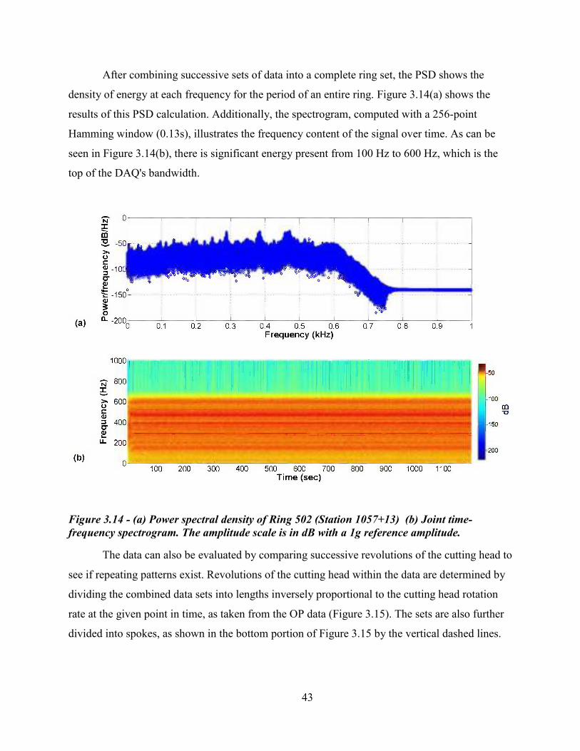
43

After combining successive sets of data into a complete ring set, the PSD shows the

density of energy at each frequency for the period of an entire ring. Figure 3.14(a) shows the

results of this PSD calculation. Additionally, the spectrogram, computed with a 256-point

Hamming window (0.13s), illustrates the frequency content of the signal over time. As can be

seen in Figure 3.14(b), there is significant energy present from 100 Hz to 600 Hz, which is the

top of the DAQ's bandwidth.

Figure 3.14 - (a) Power spectral density of Ring 502 (Station 1057+13) (b) Joint time-

frequency spectrogram. The amplitude scale is in dB with a 1g reference amplitude.

The data can also be evaluated by comparing successive revolutions of the cutting head to

see if repeating patterns exist. Revolutions of the cutting head within the data are determined by

dividing the combined data sets into lengths inversely proportional to the cutting head rotation

rate at the given point in time, as taken from the OP data (Figure 3.15). The sets are also further

divided into spokes, as shown in the bottom portion of Figure 3.15 by the vertical dashed lines.

44

Figure 3.15 - Dividing the vibration data into successive revolutions and spokes.

Using the rotation rate from the OP data stream as an input, an algorithm was developed

to segregate the data sets and produce a stacked representation of subsequent revolutions.

Applying this algorithm to the data sets of Ring 502 yields a clear pattern in the stacked data,

which can be seen in Figure 3.16. This pattern is a small decrease in amplitude between the 3-5

second period, for each of the 46 stacked revolutions. This result is likely due to some

eccentricity in the rotating cutting head. This does, however, indicate that events that are created

by object striking the cutting head will appear in successive revolutions.

To investigate further if events show up in successive revolutions, the data for Ring 684

is evaluated. As can be seen in Figure 3.17, there are a number of spikes present in the vibration

data, along with several gaps in the data. During this ring the machine tunneled through an

existing construction area and the soil had been previously excavated and then replaced with

controlled density fill (CDF), which is similar to a weak concrete. A cross section of the machine

45

and its relative position to the previous construction and CDF can be seen in Figure 3.18. This

material is considered hazardous waste, and therefore must be disposed of accordingly, which

required inspections during excavation, and the reason for the breaks in the data set at the 2, 21

and 42 minute marks. This also complicates the continuity of analyzing consecutive revolutions,

therefore, only the data after the 42 minute mark was considered in this analysis.

Figure 3.16 - 46 stacked revolutions of accelerometer a4L data during Ring 502

Considering only data after the 42 minute mark, yields 25 successive revolutions and

numerous spikes, as shown in Figure 3.19(a). A closer look, near the 29 second mark, reveals

spikes in very close proximity, as shown in Figure 3.19 (b). However, these spikes are not in

successive revolution, but are from revolution 84 and then revolution 90, which might indicate

that a tooth on the cutting head struck an inclusion, and broke a chunk off. Then, when the

machine advanced forward and six revolutions later, the cutting head struck the remainder of the

46

inclusion. As shown in Figure 3.17, the machine's advance rate was approximately 75 mm/min,

therefore during the six revolutions, the machine advance a linear distance of approximately 250

mm.


sensor a1 in the transverse (T), vertical (V) and longitudinal (L) directions overlaid with their

respective RMS signals.

Another indication of the cutting head striking an object is the impulse like response

illuminated in the spectrogram of Figure 3.20(b), where the event excites the entire frequency

band.

47

Figure 3.18 - Approximate location of TBM during Ring 684 (Station 1048+04), showing the

TBM's proximity to the CDF and existing construction of Interstate 5.

Figure 3.19 - (a) The stacked a1L accelerometer data showing revolutions 73:97 for Ring 684

(Station 1048+04) (b) zoomed section showing spikes in revolution 84 and 90, respectively.

48

Figure 3.20 - (a) Operational Data (OP) of Ring 684 (Station 1048+04) (b) joint time-

frequency spectrogram of a1T where the period between 15-28 seconds is the cutting head

changing directions and the sloping line (22-28 second range) is the cuttinghead increase in

RPM and the spike at 123 seconds. The amplitude scale is in dB with a 1g reference

amplitude.

Further investigation of this impulse, in the time domain, reveals that there are three

spikes, as can be seen Figure 3.21(b). The time difference between the first and second spikes is

0.4 seconds, which at 1.72 rpm, could be the time elapsed between a scraper bit on either side of

the spoke or a pre-cutting bit and a scraper on a single spoke. The time difference between the

second and third spikes is 5.8 seconds, which at 1.72 rpm, is roughly the time that would elapse

between teeth on adjacent spokes striking the same object.

49

Figure 3.21 - (a) Several spikes found in the 76th revolution of the excavation of Ring 684

(Station 1048+04) (b) zoomed section identifying three spikes.

3.5.3 Cross Correlation

Another time series method that complements the stacked revolution data is cross

correlation. In cross correlation, the relative phase of two signals is calculated in order to

determine the lag of one signal versus the other. In this method, successive revolutions are cross-

correlated to investigate corresponding periodicity. To evaluate this method, the data from Ring

601 was chosen. As can be seen in Figure 3.22, there are periods in the data set where distinct

differences in both the OP data and the vibration data are observed. However, the rotation rate

appear to remains constant.

50

Figure 3.22 - (a) Operational data (OP) and (b) sensor 1 acceleration time histories during the

excavation of Ring 601 (Station 1052+19).

Cross correlating the successive revolutions of Ring 601 illuminates variations in the

periodicity, which can be attributed to the rotation rate. First, comparing revolutions one with

revolution two, where the rotation rate is known to increases from zero to 1.86 rpm produces a

very skewed cross correlation plot, as shown in Figure 3.23(c).

Next, comparing revolution four with revolution five, produces nearly zero lag in the

peak value of the cross correlation plot as shown in Figure 3.24(c). This indicates that the two

principal frequencies are well aligned. The cross correlation also exhibits symmetry about the

zero lead/lag point, which strongly suggests that the two successive revolutions have a similar

signature. However, comparing the time series of revolution 4 with revolution 5, as shown in

Figure 3.24(a) and Figure 3.24(b) respectively, the similarity is difficult to discern.

51

Figure 3.23 - Vibration data from Ring 601 (Station 1052+19) accelerometer a1L, where (a) is

revolution #1 (b) is revolution #2, and (c) is the cross correlation between revolution 1 &2.

Figure 3.24 - Vibration data from Ring 601 (Station 1052+19) accelerometer a1L, where (a) is

revolution #4 (b) is revolution #5, and (c) is the cross correlation between revolution 4 &5.

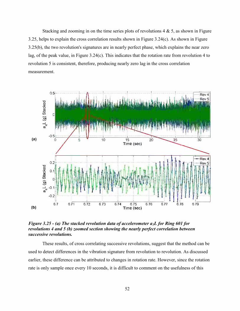
52

Stacking and zooming in on the time series plots of revolutions 4 & 5, as shown in Figure

3.25, helps to explain the cross correlation results shown in Figure 3.24(c). As shown in Figure

3.25(b), the two revolution's signatures are in nearly perfect phase, which explains the near zero

lag, of the peak value, in Figure 3.24(c). This indicates that the rotation rate from revolution 4 to

revolution 5 is consistent, therefore, producing nearly zero lag in the cross correlation

measurement.

Figure 3.25 - (a) The stacked revolution data of accelerometer a3L for Ring 601 for

revolutions 4 and 5 (b) zoomed section showing the nearly perfect correlation between

successive revolutions.

These results, of cross correlating successive revolutions, suggest that the method can be

used to detect differences in the vibration signature from revolution to revolution. As discussed

earlier, these difference can be attributed to changes in rotation rate. However, since the rotation

rate is only sample once every 10 seconds, it is difficult to comment on the usefulness of this

53

method at intervals below 0.1 Hz. Nevertheless, this approach offers a mechanism that could be

automated to detect gross changes in rotation rate.

3.6 Summary

Over the three generations of the BDS system, it has matured into a robust measurement

system. In its evolution, it has become virtually maintenance free, autonomous, and has produced

a wealth of data to investigate the posed research questions. The analysis of these data sets have

produced a number of interesting results, such as the ability to compare the vibration values with

the OP data and the ability to find events in successive revolutions.

54

CHAPTER 4

OPERATIONAL MODAL ANALYSIS

In order to understand how a TBM responds to external excitation, a series of

experimental tests were performed. The goal of these tests was to investigate the frequency

response so that it could be used to characterize the dynamics of a TBM and used to understand

the vibration response during operation.

There are generally two experimental methods that can be employed for characterization,

experimental modal analysis and operational modal analysis (OMA). Both of these methods

require that three characteristics to be true: 1) the system is linear, 2) the system is time invariant,

and 3) the system will exhibit reciprocity, or that the same frequency response can be obtained

by reversing the input with the output. For this thesis, only OMA was explored, because

experimental modal analysis is difficult to perform once the TBM was in operation and

underground. The following will briefly explain OMA, its implementation in the Seattle project,

and the various results obtained.

4.1 Operational Modal Analysis (OMA)

OMA is similar to traditional modal analysis except that the results are obtained without

measuring the system's input. Data is collected for extended periods of time and the data often

appears to represent a stochastic process. In this research, the vibration data from the bulkhead of

the Seattle TBM was grouped by rings and then compared on a ring by ring basis. Ring 502 data

can be seen in Figure 4.1, where a ring represents about 1.5m of linear excavation.

The goal of OMA is to provide a mechanism to compare the operating frequencies and

their amplitudes observed during each ring. Then, if the values remain the same, we can

hypothesize the geology is the same and if it changes, then either the system has changed or the

input (geology) has changed. To illustrate this concept we begin by comparing the vibratory

signature and spectrogram for sequential rings. These two rings are 502 and Ring 507, which are

separated by roughly 7.5m, and presumably excavating in similar geological conditions. As

shown in Figure 4.2, these successive rings appear to exhibit similar characteristics, in both the

55

time series data and the frequency domain data. Therefore a more quantitative method, like

OMA, needs to be employed to investigate how similar these sets are.

Figure 4.1 - Vibration data from Ring 502 (Station 1057+13) for sensor a1 in the transverse

(T), vertical (V) and longitudinal (L) directions overlaid with their respective RMS signals

Figure 4.2 - Vibration levels at the beginning of Ring 502 (Station 1057+13) and at the end of

Ring 507 (Station 1056+88). (a) shows the vertical acceleration starting to rise as the cutting

head begins to rotate and contacts the face, then fall as the excavation is complete. (b) shows a

spectrogram of the vertical acceleration where the sloping line (2-10 second range) illuminates

the increase in RPM and then the opposite (56-59 second range) as the cutting head comes to

a stop. In (b) the scale is in dB with a 1g reference.

56

One technique for performing OMA is frequency domain decomposition (FDD) [8],

which decomposes a spectral matrix into modal frequency values using singular value

decomposition (SVD), shown in Equation (4.1). The reference by Baker [12] helped in

understanding SVD. This technique is performed on a matrix of spectral data X, where each

rows is the spectral content of a single accelerometer record.

(4.1)

X = M x N matrix of spectral data

U = M x M real or complex unitary matrix

= M x N rectangular diagonal matrix, where the diagonal entries are nonnegative and known as

the singular values (σ1, σ2...σn) of X

VH =N x N matrix, where H represents the conjugate transpose

The method produces two desirable results, the singular value (SV), which are the

amplitude values (σ) at each frequency and the eigenvector (U) at each frequency. A step by step

approach of FDD follows below:

1) assemble a matrix of data, where the rows are each channel of data and the columns are the

data associated with each channel, which yields an M x N matrix.

2) calculate the CPSD, which yields N, M x M matrices, where the N's are the values at each

frequency for each PSD.

3) Compute the complex conjugate of the CPSD.

4) Compute the SVD of each M x M matrix at each frequency, which yields the σ1 value at each

frequency.

Performing FDD on the entire data set (which includes starts and stops) of Rings 502 and

Ring 507 yields values that can more succinctly be compared on a ring by ring basis. As can be

seen in Figure 4.3, the dominant frequencies are the same, however the largest amplitude of Ring

502 is nearly twice that of Ring 507. Based on the proposed hypothesis, the difference in

57

amplitude was hoped to be related to changes in the geology. However, the SVD amplitude

results are not scaled, therefore making the amplitude comparison, between rings, not

meaningful. The primary reason that it is felt that the amplitude values are not comparable is that

each data set's length is unique and this influence has not been accounted for or characterized.

Figure 4.3 - (a) SV of the longitudinal accelerometers for Ring 502 (Station 1057+08), (b) SV

of the longitudinal accelerometers for Ring 507 (Station 1056+88)

Exploring this hypothesis further and performing FDD on Ring 358 and Ring 502 yields

different results. The primary difference in the results is the fundamental frequency, where Ring

358 is near 390 Hz and Ring 502 is near 470 Hz, which is approx. a 20% difference. These

results are shown in Figure 4.4. Comparing the difference between these two rings reveals that

there is also approximately a 20% difference in the TBMs rotation rate N during the two

excavations, where Ring 358's N = 1.74 rpm and Ring 502's N = 2.17 rpm.

This relationship to rotation rate was further explored by plotting the dominant

frequencies observed in the response from each of the four sensors, and their respective

responses in each of the T,V, and L directions. All results are included in Figure 4.5, including

stops, starts and various transitions associated with typical tunneling. Each data point in Figure

4.5 reflects the response from 80 seconds of vibration data vs. the average rotation rate during

this time period and are not the results of FDD. A number of interesting observations can be

made from these plots, which are shown in Figure 4.5. One interesting observation, that supports

our previous finding, is that the dominant frequency in each of the T, V and L directions exhibit

a somewhat linear relationship with rotation rate, albeit with significant scatter. Another

58

interesting observation is that there are a number of outliers, especially near the lower rotation

rates. These outliers most likely can be attributed to the stops and starts of the TBM, because

they exist below the lower rotation rate threshold of the TBM's typical operating regime. Yet

another interesting observation is the spreading or variance that occurs in the higher rotation

rates, especially in the transverse and vertical directions.

Figure 4.4 - (a) SV of the longitudinal accelerometers for Ring 358 (Station 1064+32), (b) SV

of the longitudinal accelerometers for Ring 502 (Station 1057+08)

Figure 4.5 - (a) Plot of the fundamental frequency vs. rotation rate for the four accelerometers

in the Transverse direction. (b) Plot of the fundamental frequency vs. rotation rate for the four

accelerometers in the vertical direction. (c) Plot of the fundamental frequency vs. rotation rate

for the four accelerometers in the longitudinal direction.

59

Looking more closely at the results presented in Figure 4.5(c), the longitudinal direction

appears to have the strongest linear relationship. Performing a linear fit on the longitudinal data

set confirms that there is in fact a linear relationship with significant scatter, as shown in Figure

4.6.

Figure 4.6 - Linear fit of the fundamental frequency vs. rotation rate for the accelerometers in

the longitudinal direction.

The data is rather noisy, but the four accelerometers appear to agree with the linear

dependence. Using SVD on the set de-noises the data and confirms that each measurement's

fundamental frequency has a linear dependence on the rotation rate. The results of the SVD are

shown in Figure 4.7.

Using the results from the two linear equations, the percent error vs. the measured valued

can be calculated. As can be seen in Table 5, both results yield similar results and their errors

are less than 5%.

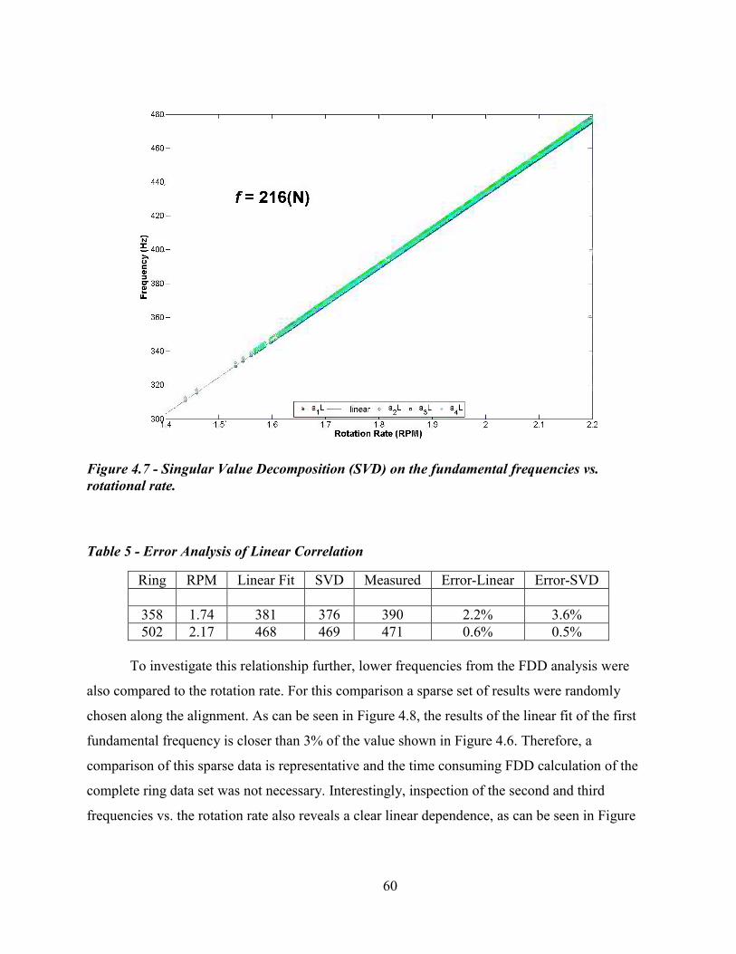
60

Figure 4.7 - Singular Value Decomposition (SVD) on the fundamental frequencies vs.

rotational rate.

Table 5 - Error Analysis of Linear Correlation

Ring RPM Linear Fit SVD Measured Error-Linear Error-SVD

358 1.74 381 376 390 2.2% 3.6%

502 2.17 468 469 471 0.6% 0.5%

To investigate this relationship further, lower frequencies from the FDD analysis were

also compared to the rotation rate. For this comparison a sparse set of results were randomly

chosen along the alignment. As can be seen in Figure 4.8, the results of the linear fit of the first

fundamental frequency is closer than 3% of the value shown in Figure 4.6. Therefore, a

comparison of this sparse data is representative and the time consuming FDD calculation of the

complete ring data set was not necessary. Interestingly, inspection of the second and third

frequencies vs. the rotation rate also reveals a clear linear dependence, as can be seen in Figure

61

4.8. This further supports the conclusion that the responses are not the resonant response of the

TBM's structure and are strongly coupled to the rotation rate of the machine.

Figure 4.8 - Plot of the top three SV frequencies vs. rotation rate, illustrating a strong linear

dependence on rotation rate.

Finally, normalizing the fundamental frequencies by the rotation rate, reveals a strong

correlation to rotation rate, as can be seen in Figure 4.9. In Figure 4.9, there exist a number of

outliers that are likely due to the stops, starts and variations of normal tunneling.

To better understand if the outliers shown in Figure 4.9 are caused by the stops, starts and

variations of normal tunneling, the sparse results from the FDD analysis were normalized by

rotation rate. As can be seen in Figure 4.10, this normalization nearly eliminates the outliers and

provides more conclusive evidence that the frequency response is coupled to the rotation rate of

the TBM in the three largest frequencies.

62

Figure 4.9 - Plot showing the fundamental frequencies of the four longitudinal accelerometers

normalized by rotation rate.

Figure 4.10 - Plot showing the top three SV frequencies of the longitudinal accelerometers

normalized by rotation rate.

63

4.2 Summary

There are two main findings that can be taken from this chapter. First, that FDD provides

a very succinct method for comparing the largest three operational frequencies from ring to ring.

The amplitudes of the SV, however, are not scaled and until a relationship can be developed,

giving meaning to the amplitude, their values should not be compared. Second, there exists a

strong coupling between the measured frequency response and the rotation rate of the TBM. The

results indicate that this coupling cannot be explained by traditional forced response theory. The

primary reason being that the frequency shifts with rotation rate. In addition, the same results

also shows that the measured response is not a result of free vibration, because the measured

frequency is not constant and changes with time or more importantly, rotation rate.

64

CHAPTER 5

MACHINE VIBRATION AND ITS RELATIONSHIP

TO GROUND CONDITIONS

This chapter was submitted to the journal Tunneling and Underground Space Technology

(TUST). The goal of this paper was to introduce the collected passive vibration data and pair it

with the operating data. To accomplish this, the vibration data was continuously collected along

with TBM operating parameters, e.g., torque, thrust, face pressure, advance rate, etc. This data,

together with geological information from the project, were then analyzed to determine the

nature of TBM vibration (in 3 dimensions), its relationship to operating parameters, and its

relationship to geology and ground conditions. Further, machine learning was also used to

investigate vibration, operating parameters and ground conditions. The results for the machine

learning investigation can be found in Appendix F.

5.1 Site Geology

Six major glacial events with intervening non-glacial erosion and depositional periods

produced the overlapping gravels, sands, silts, clays and tills along the U230 alignment, as

shown in Figure 5.1. Geologic description of this project can be divided into fluvial deposits,

glacial deposits, lacustrine and glaciolacustrine deposits, all of which have been glacially

over‐ridden and are therefore very overconsolidated.[13] The overburden varied from a

minimum of 4.2 m under Interstate 5 (Station 1046) to over 40 m (Station 1060). The entire

tunnel alignment has a steep, curved downhill grade (4.8%). SI units are used throughout the

paper except for station and elevation where feet were used throughout all project documents. In

additional, while data was collected along the entire 1 km alignment, only data collected in the

second half of the tunnel (Station 1065 to Station 1045) will be presented in this study. The

primary reason for this being that measurement parameters were being adjusted in the first half

of the project.

5.2 Vibration Data

Vibration data is first presented for a few typical excavation cycles. Each excavation

cycle corresponds to a single ring of precast reinforced concrete segmental lining, where the ring

designation is the current ring being constructed and the Station designation is the nose cone of

65

the cutting head, approx. 7.5 m or the equivalent length of five rings ahead of the ring being

constructed. The excavation time of each 1.5 m long ring varied from 20 - 60 min (approximate).

Figure 5.2 shows the triaxial acceleration responses (in the L, T and V directions) at sensor

location 1 during the excavation of ring 502 through low plasticity clay (Station 1057+13)

together with cutting head rotation rate (N), advance rate (AR), torque (T) and thrust (F).

Acceleration levels at the three other bulkhead sensor locations were similar in behavior to

location 1 and are not presented here. The mean or DC offset was subtracted from the vibration

data. Vibration data was recorded at a sampling rate of 2 kHz while the OP data was recorded at

0.1 Hz (every 10 s).

Figure 5.1 - Geological conditions along the U230 tunnel project [14]

TBM operation during excavation was governed by torque level and proceeded as

follows. The operator set the cutting head rate of rotation to a desired level, typically N = 1.8-2.2

rpm, and then increased the advance rate until 70% of the maximum rated torque (4160 kN-m)

was reached. Subsequently, if the measured torque decreased, the advance rate was increased to

raise the torque level back to the desired 70%, and vice versa. Cutting head rotation rate also

plays an important role in setting torque levels, however, the relationship is less intuitive and not

the typical means for controlling the torque. For example, if the advance rate was held constant

and the rotation rate was decreased, the resultant torque would increase and vice versa.

66

Essentially, by decreasing the rotation rate for a constant advance rate, the cutting head is

excavating more ground per revolution, thus increasing torque. Generally, for clay or silty

ground, the cutting head rotation rate is increased to cut a thinner portion of the face and

facilitate the mixing process inside the chamber. Conversely, for particles larger than silt

(namely sand and gravel), the cutting head rotation rate is typically lowered to both remove more

material and maximize the available torque.

As shown in Figure 5.2, magnitudes of OP data were fairly constant during ring 502

excavation, with the exception of a slight increase in advance rate. This was typical of many ring

excavations. Measured torque exhibited mild fluctuation, where the torque coefficient of

variation (cv = /µ) was 10%. Conversely, the cutting head rotation rate was more deterministic

and characterized by a periodicity equal to the time of one rotation. Also shown in Figure 5.2, the

longitudinal acceleration a1L exhibited the largest observable amplitude, followed by a1V and

a1T. As will be discussed later, this order of vibration magnitude was not always the case.

Bulkhead vibration was found to be stochastic in nature. To this end, root mean square

(RMS) amplitudes a1LRMS, a1VRMS and a1TRMS are also shown in Figure 5.2. Here, each RMS

amplitude was determined from 20 seconds of vibration data, equivalent to approximately one-

half of a complete cutting head rotation. The average a1LRMS (0.06g) was proportionally much

greater than a1VRMS (0.05g) and a1TRMS (0.04g) than is evidenced by comparison of the full

waveform data. a1TRMS generally remained constant during ring 502 excavation while a1LRMS

and a1VRMS increased slightly until 15-16 min then remaining constant. These changes coincide

with the slight increase in advance rate. In general, ring 502 excavation yielded relatively

uniform OP and vibration response.

The stochastic nature of bulkhead vibration is further illustrated in Figure 5.3 where the

waveform and histograms of a1L, a1V and a1T data are presented. Each a1L, a1V and a1T

histogram exhibits Gaussian behavior with the standard deviation in a1L, a1V and a1T data

equaling the average RMS amplitude. Figure 5.3 also presents a1LRMS, a1VRMS and a1TRMS

calculated every 0.625 s, a duration much shorter than the approximate 40 seconds required to

complete a single cutting head rotation. These a1LRMS, a1VRMS and a1TRMS histories reveal a clear

oscillation pattern with a characteristic frequency equal to the cutting head rate of rotation. The

magnitude of RMS oscillation is noticeably different, with a1LRMS > a1VRMS > a1TRMS. These will

67

be described in greater detail below. The cutting head is a radially symmetric body and in theory

should not cause the observed fluctuations. However any number of the following scenarios

could be the cause of the observed periodicity: the asymmetric trapping of soil in cutting head

openings, uneven wear on the cutters, the position of the TBM in the curved alignment, uneven

injection of soil conditioning through the cutting head, and the rotating mass of soil in the mixing

chamber. Variability in cutting head rotation rate (see Figure 5.2) may also contribute to the

oscillating RMS vibration.

Figure 5.2 - (a) Operational Data (OP) and (b) sensor 1 acceleration time histories (full

waveform and RMS amplitude) during excavation of Ring 502 (Station 1057+13).

Figure 5.4 looks more closely at time and frequency domain a1V response during

initiation of excavation for ring 502 (Station 1057+13) and during conclusion of ring 507

excavation (Station 1056+88). Figure 5.4b presents a joint time-frequency analysis (spectrogram)

illustrating the frequency content of the signal with time. A 256 point hamming time window

(0.13 s length) was used in the spectrogram. Meaningful signal was observed below 500 Hz. The

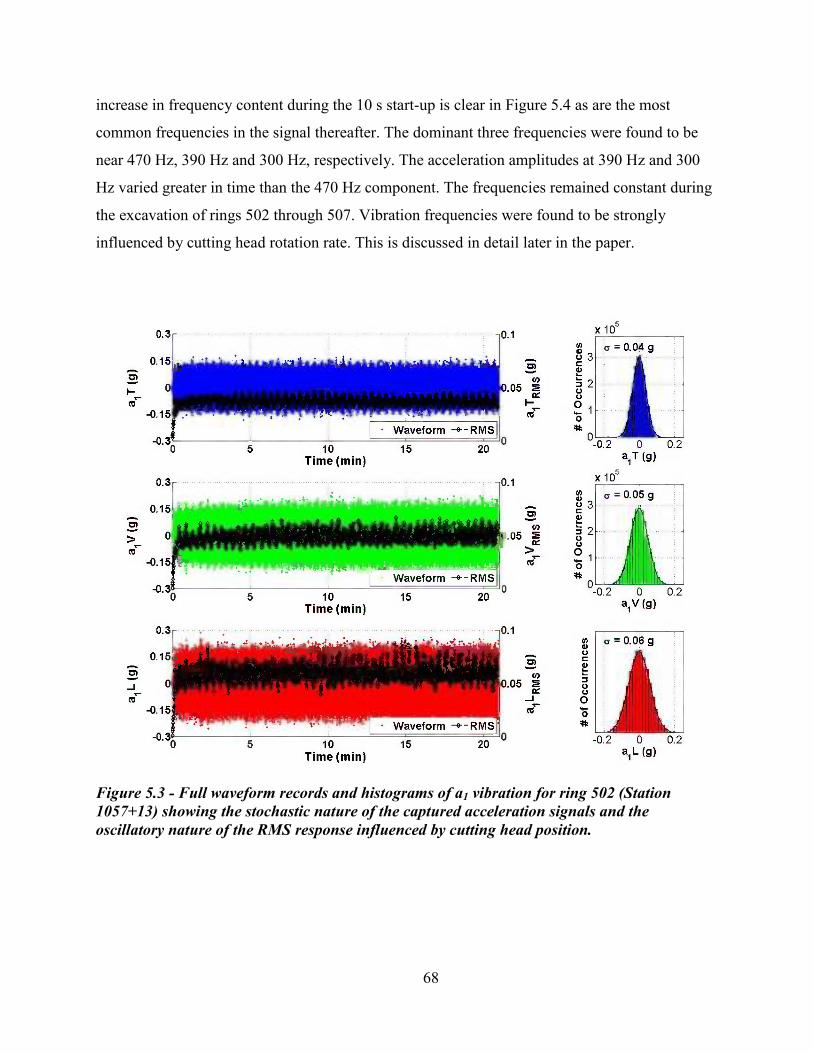
68

increase in frequency content during the 10 s start-up is clear in Figure 5.4 as are the most

common frequencies in the signal thereafter. The dominant three frequencies were found to be

near 470 Hz, 390 Hz and 300 Hz, respectively. The acceleration amplitudes at 390 Hz and 300

Hz varied greater in time than the 470 Hz component. The frequencies remained constant during

the excavation of rings 502 through 507. Vibration frequencies were found to be strongly

influenced by cutting head rotation rate. This is discussed in detail later in the paper.

Figure 5.3 - Full waveform records and histograms of a1 vibration for ring 502 (Station

1057+13) showing the stochastic nature of the captured acceleration signals and the

oscillatory nature of the RMS response influenced by cutting head position.

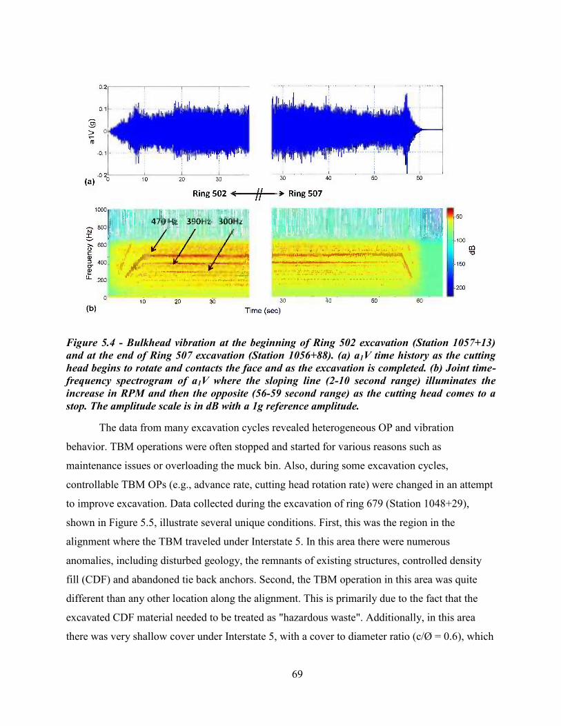
69

Figure 5.4 - Bulkhead vibration at the beginning of Ring 502 excavation (Station 1057+13)

and at the end of Ring 507 excavation (Station 1056+88). (a) a1V time history as the cutting

head begins to rotate and contacts the face and as the excavation is completed. (b) Joint time-

frequency spectrogram of a1V where the sloping line (2-10 second range) illuminates the

increase in RPM and then the opposite (56-59 second range) as the cutting head comes to a

stop. The amplitude scale is in dB with a 1g reference amplitude.

The data from many excavation cycles revealed heterogeneous OP and vibration

behavior. TBM operations were often stopped and started for various reasons such as

maintenance issues or overloading the muck bin. Also, during some excavation cycles,

controllable TBM OPs (e.g., advance rate, cutting head rotation rate) were changed in an attempt

to improve excavation. Data collected during the excavation of ring 679 (Station 1048+29),

shown in Figure 5.5, illustrate several unique conditions. First, this was the region in the

alignment where the TBM traveled under Interstate 5. In this area there were numerous

anomalies, including disturbed geology, the remnants of existing structures, controlled density

fill (CDF) and abandoned tie back anchors. Second, the TBM operation in this area was quite

different than any other location along the alignment. This is primarily due to the fact that the

excavated CDF material needed to be treated as "hazardous waste". Additionally, in this area

there was very shallow cover under Interstate 5, with a cover to diameter ratio (c/Ø = 0.6), which

70

required careful TBM operation to reduce the risk of damage to Interstate 5. As shown early in

Figure 5.5, the TBM was stopped and started twice to evacuate the "clean" muck and to prepare

to isolate the CDF/soil mixture (for hazardous waste treatment).

During excavation from 29-52 min, the cutting head rotation rate slightly decreased while

torque and thrust steadily increased and the advance rate remained constant. In this section, the

TBM was excavating previously constructed fill, which is often not evenly compacted and

therefore explains the erratic vibration values. At 53 min, there are several captured spikes that

are most likely the cutting head encountering the abandoned tieback anchors. At 56 min, the

cutting head is stopped and the direction is reversed to correct machine rolling beyond a

specified inclination, to assisting in navigating the TBM, etc. The vibration become more steady

as the TBM becomes fully engaged with the homogeneous CDF. It is worth noting that OPs for

ring 679 excavation are much different than ring 502 given the difference in strength of the CDF

(3.5-9 MPa) vs. the ML/CL soil (1 MPa). Most notably, the torque for ring 679 excavation

through CDF material is nominally twice that of ring 502 excavation through ML/CL soil, while

the bite per cutting head revolution (= AR/N) of ring 679 excavation is nominally 50% of ring

502 excavation, i.e., much higher torque per bite in the CDF.


74 minute excavation of Ring 679 (Station 1048+29). See Figure 1 for L, T and V directions.

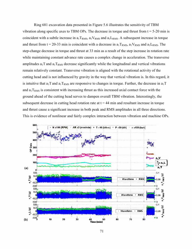
71

Ring 681 excavation data presented in Figure 5.6 illustrates the sensitivity of TBM

vibration along specific axes to TBM OPs. The decrease in torque and thrust from t = 5-20 min is

coincident with a subtle increase in a1TRMS, a1VRMS and a1LRMS. A subsequent increase in torque

and thrust from t = 20-33 min is coincident with a decrease in a1TRMS, a1VRMS and a1LRMS. The

step-change decrease in torque and thrust at 33 min as a result of the step increase in rotation rate

while maintaining constant advance rate causes a complex change in acceleration. The transverse

amplitudes a1T and a1TRMS decrease significantly while the longitudinal and vertical vibrations

remain relatively constant. Transverse vibration is aligned with the rotational activity of the

cutting head and is not influenced by gravity in the way that vertical vibration is. In this regard, it

is intuitive that a1T and a1TRMS are responsive to changes in torque. Further, the decrease in a1T

and a1TRMS is consistent with increasing thrust as this increased axial contact force with the

ground ahead of the cutting head serves to dampen overall TBM vibration. Interestingly, the

subsequent decrease in cutting head rotation rate at t = 44 min and resultant increase in torque

and thrust cause a significant increase in both peak and RMS amplitudes in all three directions.

This is evidence of nonlinear and fairly complex interaction between vibration and machine OPs.

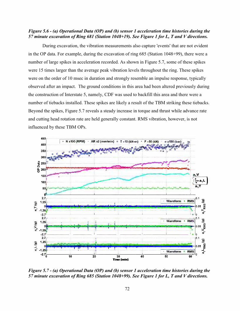
72



During excavation, the vibration measurements also capture 'events' that are not evident

in the OP data. For example, during the excavation of ring 685 (Station 1048+99), there were a

number of large spikes in acceleration recorded. As shown in Figure 5.7, some of these spikes

were 15 times larger than the average peak vibration levels throughout the ring. These spikes

were on the order of 10 msec in duration and strongly resemble an impulse response, typically

observed after an impact. The ground conditions in this area had been altered previously during

the construction of Interstate 5, namely, CDF was used to backfill this area and there were a

number of tiebacks installed. These spikes are likely a result of the TBM striking these tiebacks.

Beyond the spikes, Figure 5.7 reveals a steady increase in torque and thrust while advance rate

and cutting head rotation rate are held generally constant. RMS vibration, however, is not

influenced by these TBM OPs.



73

The final presented ring excavation data set in Figure 5.8 shows the complicated

influence of cutting head rotation rate. As shown in Figure 5.8 there is a strong correlation

between the RMS vibration value and RPM. Specifically, as the RPM increases the RMS

vibration values decrease. This behavior indicates that the nominally measured response is being

driven by the rotation rate of the cutting head.



However, the measured responses also captures unique events, such as those highlighted

in Figure 5.9, where several spikes occur at t=7 min. These impulse type responses further shows

the complicated interaction between the machine and the encountered geology. If the cause of

these responses could be more clearly identified or linked to progressive damage of the cutting

head, then the added value of these types of measurements would be very clear.

74

Figure 5.9 - (a) time history data from accelerometer a1L during the 29 minute excavation of

Ring 698 (Station 1047+33). (b) zoomed section showing multiple captured spikes.

5.3 Vibration Signature along the Alignment

To explore TBM vibration behavior broadly, Figure 5.10 presents key OP data as well as

a1LRMS, a1VRMS and a1TRMS along approximately 610 m (2000 ft) of the alignment. The

geological interpretation for the site is also shown. It should be mentioned that this geology was

not mapped during tunneling and actual conditions might have deviated considerably from this

estimation. In Figure 5.10, both the OP and vibration data were averaged to produce one value

for each parameter per ring. Broadly, torque, thrust, and face pressure decreased as the TBM

excavated (from right to left) through predominantly ML soils, then CL/ML soils with some CH,

and then CH soils from Station 1053 on. A cutting head rotation rate = 2.2 rpm was maintained

for most of the alignment. The rotation rate was lowered in a number of areas (while maintaining

the advance rate), and as a consequence, measured torque levels increased.

75

Unfortunately there were only seven exploration borings performed in this region and

nearly all of the borings yielded unique geology. These borings, their soil designation and the

standard deviation of the a1L vibration measurement near the boring location are shown in Figure

5.10c. As can be seen in Figure 5.10c the vibration values generally suggests the following: Clay

+ Silt produces higher RMS vibration than just Clay. In addition, Clay (CH) produces higher

RMS vibration than Clay (CL). Regrettably, with only the seven boring location, it is difficult to

make more than a general statement about the correlation of RMS vibration to a specific geology

type. However the TBM vibration levels clearly varied along the alignment as shown in Figure

5.10c. There are numerous zones where RMS acceleration increased significantly (by a factor of

two or more), namely near Stations 1045, 1046, 1048, 1052, 1061 and 1064. The increased RMS

values at Stations 1045, 1046 and 1048 can be attributed to the previously discussed disturbances

in the native geology, near the Interstate 5 corridor and presence of tieback anchors and CDF.

There are however three locations that exhibited elevated RMS vibration levels, specifically

Stations 1052, 1061 and 1064. Comparing the geologic profile shown in Figure 5.10b and the

RMS values shown in Figure 5.10c, there is a strong argument to suggest that vibration levels

increase where there are transitions of soil types. While none of the borings are exactly located in

these regions, the OP data shown in Figure 5.10a support the claim that there is a distinct

geology transition in these zones.

Along the majority of the alignment, RMS vibration levels were found to be greatest in

the longitudinal direction and lowest in the transverse direction. However, a1TRMS exceeded

a1LRMS during most of the zones where elevated accelerations were observed (Figure 5.10d). A

similar behavior was observed in the vertical acceleration in that a1VRMS exceeded a1LRMS during

most of the zones where elevated accelerations were observed. In four areas - near Stations 1045,

1048, 1061 and 1064 – the vertical and transverse bulkhead acceleration levels were greater than

the longitudinal, a trend that is considerably different than everywhere else along the alignment.

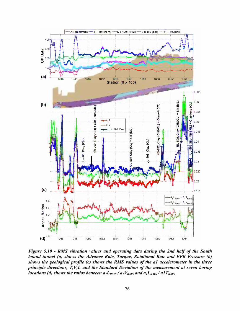
76

Figure 5.10 - RMS vibration values and operating data during the 2nd half of the South

bound tunnel (a) shows the Advance Rate, Torque, Rotational Rate and EPB Pressure (b)

shows the geological profile (c) shows the RMS values of the a1 accelerometer in the three

principle directions, T,V,L and the Standard Deviation of the measurement at seven boring

locations (d) shows the ratios between a1LRMS / a1VRMS and a1LRMS / a1TRMS.

77

The interplay between bulkhead vibration, TBM OPs and ground conditions is

understandably complex. With many variables involved, it is difficult to establish clear cause and

effect. An evaluation of the peak vibration areas suggests that TBM vibration is influenced by

both OPs and ground conditions. It is evident from inspection of the OP data alone that torque

and thrust are influenced by ground conditions. For example, with the exception of the CDF near

Station 1048, the CH soil from Stations 1047-1051 generate less torque and thrust than the MH

and CL soil at higher stations (for equal N).

It is also apparent that machine OPs influence bulkhead vibration. An increase in torque

caused by the geology creates greater acceleration in the plane of the cutting head, namely the T-

V directions, and little increase in the L direction. Conversely, a decrease in cutting head rotation

rate alone yields a proportional increase in a1LRMS, a1VRMS and a1TRMS. Therefore, the ratios

a1LRMS / a1VRMS and a1LRMS / a1TRMS rather than the magnitudes of a1LRMS, a1VRMS and a1TRMS

provide valuable information about ground conditions.

One additional way to illustrate the influence of geological conditions is to compare

vibration levels with specific energy (SE). Described in Equation (5.1), SE has long been used in

drilling communities and more recently in tunneling [2][3] to combine OPs [15]. It has been

shown that SE correlates with geological properties such as hardness and shear strength.

Extrapolating from this, SE is presented in Figure 5.11 as a surrogate for shear strength of the

soils. A comparison of SE with the acceleration records reveals a relatively strong correlation.

(5.1)

where the terms of Equation (5.1) are defines as:

SE = Specific Energy (kPa)

F = Thrust (kN)

A = Tunnel Cross Sectional Area (m2)

N = Cutting head Rotation Rate (RPM)

T = Torque (kN-m)

78

Figure 5.11 - Comparison of Specific Energy with RMS vibration in the a1V direction.

5.4 Summary

In this study, an earth pressure balance (EPB) TBM was outfitted with accelerometers

and monitored during approximately 1 km of tunneling through Seattle glacial soils. The

vibration data were continuously collected along with TBM operating parameters, e.g., torque,

thrust, face pressure, advance rate, etc. This data, together with geological information from the

project, were then analyzed to determine the nature of TBM vibration (in 3 dimensions), its

relationship to operating parameters, and its relationship to geology and ground conditions.

Bulkhead vibration levels in the longitudinal, vertical and transverse directions typically

ranged from 0.1 to 0.5 g, with periodic spikes in vibration exceeding 2.5g. Vibration levels

varied considerably along the alignment but showed strong correlations to changes in ground

conditions, especially where there were transitions in soil types. These findings were supported

by the classical comparison of operating parameters to changing soil condition, yet offer

additional insight into the machine/soil interaction. Additionally, a comparison of the recorded

79

accelerations to the Specific Energy, which is used as a surrogate for shear strength of soil, also

exhibits a strong correlation. These discoveries offer insight into the complicated interaction

between the TBM and its environment. Moreover, these results provide a real-time means for

the operator to make an informed decision about changing ground conditions.

80

CHAPTER 6

PRINCIPAL MOTION

To aid in the interpretation of the experimental results, a technique called Principal

Motion (PM) will be explored. The concept behind this technique is transforming physical

measurements onto modal space and then transforming them back to the physical domain. This

process results in a purposeful loss of information, that yields a set of results that are filtered by

the transformation [16], [17]. The goal of this filtering process is to separate the flexible motion

from the rigid body motion.

6.1 Principal Motion Calculations

To perform this filtering Equation (6.1) is used to project the measured acceleration

values into modal space.

(6.1)

X = vector of quantities (accelerations) in physical (Cartesian) space

Ø = mode shapes matrix that define the rigid body motion of interest

q = vector of corresponding quantities (accelerations) in modal space

Step one in the process is defining the rigid body mode shape matrix, which defines how

the accelerometer measurements will be mapped to the rigid body modal space. There are 6 rigid

body modes, three translational in the T, V and L directions, and three rotational about T, V and

L. For this research, only four of the possible six will be considered. The four rigid body modes,

T, V, L and RL, and their orientation to the TBM can be seen in Figure 6.1. There are two reason

that the other two rigid body modes, RT and RV, are not used. First, with the current sensor layout

it is not possible to resolve rotations about T and V. Second, due to the long cylindrical shape of

the TBM the rotations about T and V are hypothesized to be small, compared to RL.

81

Figure 6.1 - Rigid body directions and their relationship to the TBM

The vector of acceleration are composed of the directional measurements from the 4

accelerometer, plus a rotational acceleration. The rotational acceleration is calculated from the

transverse and vertical acceleration components, as shown in Figure 6.2. This result in a 16 row

vector with the acceleration terms collected in the order shown in Equation (6.2).

(6.2)

The rigid body mode shape matrix is shown in Equation (6.3). The components of the

matrix are the rigid body directions T, V, L and RL. The matrix contains a sub matrix that repeats

for each three axis accelerometer. For this research, there were 4 accelerometers, therefore Ø will

be 16 x 4 matrix. In addition, each mode shape direction entry in the matrix needs to be

normalized in order to scale the rigid body modes shapes to the unit vector. This is done to scale

the unit magnitude, of each mode shape, when the coefficients are summed.

82

Figure 6.2 - Graphical illustration showing how the transverse (axT) and vertical (axV)

accelerometer measurements are combined to for the rotational acceleration (aRLx)

(6.3)

Next, to project the rigid body mode shape, the inverse of the rigid body mode shape and

the vector of accelerations are pre-multiplied, as shown in Equation (6.4). An example of the

projection calculation, with the normalized matrix rigid body shapes and the corresponding

accelerometer channel, can be seen in Equation (6.5).

(6.4)

83

(6.5)

Next, the filtered modal quantities are transformed back into Cartesian space, using

Equation (6.1). To estimate the magnitude of the rigid body motion the root mean square (RMS)

of the four sensors, in each direction, is calculated using Equation (6.6). The RMS value is also

calculated for the unfiltered accelerometer data, in each direction. This results in an RMS value

for the filtered (Xfiltered RMS) and unfiltered (Xun-filtered RMS) accelerometer values, in each of the

principal direction. Finally, a percent of the rigid body motion can be calculated through a ration

of filtered to un-filtered RMS acceleration values, as shown in Equation (6.7).

(6.6)

(6.7)

6.2 Evaluating Principal Motion with Simulated Data

In this research there are four accelerometers mounted to the bulkhead of the TBM. As

was shown in previous chapters, the bulkhead vibrates at a frequency that is coupled with the

rotation rate of the cutting head, and this content is typically dominant in the measured signal.

Therefore the objective of principal motion, in this research, is to filter the dominant response of

the bulkhead and retain the rigid body motion of the TBM. To more clearly illustrate the

application of PM, a simulation will be presented. Then data collected from the Seattle project

will be analyzed with this technique. To begin, the simulated positions of the sensor are shown in

Figure 6.3a, where the sensors are equally placed, radially around the center of the bulkhead.

Each sensor's measuring axis is aligned with the three principal directions T, V, and L.

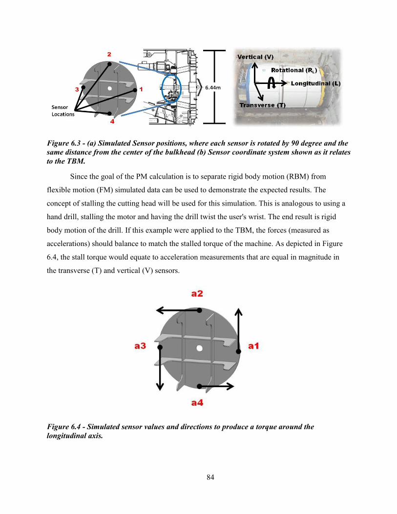
84

Figure 6.3 - (a) Simulated Sensor positions, where each sensor is rotated by 90 degree and the

same distance from the center of the bulkhead (b) Sensor coordinate system shown as it relates

to the TBM.

Since the goal of the PM calculation is to separate rigid body motion (RBM) from

flexible motion (FM) simulated data can be used to demonstrate the expected results. The

concept of stalling the cutting head will be used for this simulation. This is analogous to using a

hand drill, stalling the motor and having the drill twist the user's wrist. The end result is rigid

body motion of the drill. If this example were applied to the TBM, the forces (measured as

accelerations) should balance to match the stalled torque of the machine. As depicted in Figure

6.4, the stall torque would equate to acceleration measurements that are equal in magnitude in

the transverse (T) and vertical (V) sensors.

Figure 6.4 - Simulated sensor values and directions to produce a torque around the

longitudinal axis.

85

Using an exponentially decaying sine wave, which is a typical vibratory response, the

results of the PM calculation can be seen in Figure 6.5. As expected, the transverse and vertical

results yield 0% rigid body motion, because the force pairs are out of phase with one another and

the rotational direction yields 100% rigid body motion.

Figure 6.5 - Simulated data showing the effects of the PM filtering on data that produces a

rotational acceleration around the longitudinal axis.

Introducing noise into the simulation (5% in amplitude, 0.1 % in phase) changes the

results dramatically, as can be seen in Figure 6.6. At the simulated frequency of 350 Hz, a 0.1 %

change in phase has a larger influence than a 5% change in amplitude, and illustrates that the PM

calculations are sensitive to deviations in phase between measurement points. These noise values

were chosen by trial and error; values beyond (5% in amplitude, 0.1 % in phase) produced results

that were unintelligible. Comparing these results to the previous results (Figure 6.5) indicates

that the PM calculation is very sensitive to noise. However, the expected trend is faintly visible

in the three PM results before the signal reaches steady state, near 0.005 seconds. In both the

86

transverse and vertical traces, the signal is close to 0%, as the previous simulation showed, and

the rotational results are near100%.


produces a torque around the longitudinal axis. 5% noise has been add to the amplitude and

0.1% noise has been added to the phase of each signal.

Applying a centered moving average, to the results shown in Figure 6.6, enhances the PM

results, as shown in Figure 6.7. However, care needs to be taken in selecting the length of the

running average. For this simulation, a five point average produced the best results. An estimate

of the running average length can be calculated by Equation (6.8). In addition, although not

apparent in these results, a centered moving average can distort the beginning and end of the

processed data. This is typically referred to as the "end effects" and care should be taken when

interpreting the filtered results near the beginning and end.

87

(6.8)


produces a torque around the longitudinal axis. 5% noise has been add to the amplitude and

0.1% noise has been added to the phase of each signal and the principal motion results have

been averaged.

Next, simulations were performed to evaluate the results of the PM calculation at the

sensor's true position. As can be seen in Figure 6.8, the sensors are not equally spaced radially

about the center.

88

Figure 6.8 - Sensor locations and the coordinate system used to describe the sensor outputs

Applying a sinusoidal response to each sensor in only the vertical directions, produces an

oscillating torque about the longitudinal axis, as can be seen in Figure 6.9. However, the results

show that the calculated values for T1, T2, T3, and T4 are not equivalent. This is an important

result because it illustrates that the calculation correctly accounts for the acceleration values with

respect to their radii from the center of the TBM. Since the torque is calculated by multiplying

the acceleration times the distance and the distances are not equal, the resultant torques are

effectively normalized by their radii. In addition, because the forces applied for this simulation

were of equal magnitude, the PM calculation will not reach 100%, as shown in Figure 6.9.

Figure 6.9 - Results of the principal motion calculations, showing accelerations that produce a

net torque value will result in rigid body motion

89

6.3 Evaluating Principal Motion with Field Data

In several data sets there are spikes that occur and require an explanation. The cause of

these events are of interest for several reasons: 1) these events are neither apparent in the

operational data nor can they be explained by operating parameter changes, 2) their amplitude

and signature in the spectrogram are significantly different than what is considered normal, and

3) some of these events have occurred in areas where know geological anomalies exist. As

discussed in Chapter 3, one explanation for these spikes is that the cutting head is striking

erratics in the alignment. To further investigate these spikes, principal motion will be applied to

the field data. An example of an event that did not show up in the OP data was found in the

excavation of ring 684, and can be seen in Figure 6.10(b) near t=122 and t=130 seconds, where

two vertical bands excite nearly the entire band of measurable frequencies.

Figure 6.10 - (a) Operational data (OP) of 684 (Station 1048+04) (b) joint time-frequency

spectrogram of a1T where the period between 15-28 seconds is the cutting head changing

directions and the sloping line (22-28 second range) is the cutting head increase in RPM and

the spikes at 122 seconds and 130 seconds are the events in question. The amplitude scale is in

dB with a 1g reference amplitude.

90

These spikes are of significant amplitude, as shown in Figure 6.11, where the largest

spike is 33 times larger than the RMS value of a1T, 46 times larger than the RMS value of a1V

and 32 times larger than the RMS value of a1L.


oscillations of the largest peak shown in (a) for the a1T, a1V and a1L directions.

Applying the PM calculations to the spike, highlighted in Figure 6.11, produces results

that are similar to those shown in the simulations. As shown in Figure 6.12, the response of the

measured accelerometers, in both the transverse and vertical directions are in close proximity,

suggesting that the entire bulkhead is moving in unison or as a rigid body. The PM calculations

also support this claim, as can be seen in Figure 6.12, where the peak values are above 50%

RBM. Additionally, the PM calculations clearly show that the measured response does not

produce a "torquing" motion about the center of the machine. Theses signatures are similar to an

impulse response, which was also apparent in the spectrogram, shown in Figure 6.10(b).

91

Figure 6.12 - Results of the principal motion calculations for the big spike of Ring 684

As discussed previously, there are many captured events that are difficult to explain. In

Ring 684 there is another large spike that occurs near the 25 minute mark, as shown in Figure

6.13.


oscillations of a peak near the 25 minute mark (a) for the a1T, a1V and a1L directions.

92

Applying principal motion to the spike, shown in Figure 6.13, yields different results than

the spike shown in Figure 6.11. As can be seen in Figure 6.14, the transverse and vertical

acceleration groups are not in phase. However, in the rotational direction, the combination of the

transverse and vertical accelerometers produce a signature that would be consistent with the

machine rolling about its center, much like the "torquing" motion described in the simulations. In

addition, the PM calculations weakly support this claim, where the % RBM is larger in the areas

where the rotational accelerations are closer to being in phase.

Figure 6.14 - Results of the principal motion calculations for the spike of Ring 685near the 25

minute mark.

6.4 Summary

In this research there are many events that appear as spikes in the vibration data,

however, their cause is not apparent in the OP data. Some of these spikes are 50 times larger than

their RMS values and have appeared in regions where geological anomalies are known to exist.

To better understand the influence of these spikes, beyond traditional vibration analysis, the

93

concept of PM has been investigated and applied to this research. The simulation results of PM

in their purest form illustrate that the four sensors can provide insight into the rigid body

response of the TBM. However, as the simulations and the application of PM to field data show,

the calculations are sensitive to measurement noise and interpretation of these results is

challenging. In addition, as discussed in Chapter 2, the response could be the local bulkhead's

modal response (mode 1 of Figure 2.7) and not the response of the entire TBM (rigid body

motion), as desired. Alternatively, calculating a net rotational acceleration from the transverse

and vertical accelerometers shows the potential to detect the machine rolling as a result of the

cutting head striking an inclusion and "torquing" the machine, as illustrated in Figure 6.14.

94

CHAPTER 7

UNIVERSITY-INDUSTRY COLLABORATION IN THE UNDERGROUND

CONSTRUCTION AND TUNNELING FIELD

The underground construction and tunneling (UC&T) industry is rapidly expanding to

meet global needs.[18] This expansion is a direct response for the pursuit of major infrastructure

improvements in areas such as public transportation, water supply and storage, wastewater

transmission and mining. Examples of this growth include the East Side Access project in NYC

[19], the Chicago Deep Tunnel project [20], and the Alaskan Way Viaduct Replacement project

in Seattle, WA. [21] As with any rapidly expanding industrial field, a primary concern is meeting

the demand for qualified and trained personnel. Any technical industry looks to the academic

community to fulfill this need, and the UC&T industry is no exception. Consistent with the

literature [22], [23], [24], [25], this paper presents findings from a series of interviews with both

industry and academic players suggests that academia is not meeting this demand. Therefore, the

focus of this chapter is to explore the barriers and opportunities that affect prospects for

increasing collaboration between academia and industry in the field of UC&T.

My interest and qualifications to pursue an answer to this question come from my

experience as a graduate student interacting with the UC&T industry. This participation has

provided me with valuable insight into available pathways for the UC&T industry to collaborate

more effectively with academia. Specifically, I have participated in a summer internship as part

of the University Link Extension in Seattle, WA; I have attended both the North American

Tunneling (NAT) and Rapid Excavation and Tunneling Conference (RETC), which are the two

major industry conferences in the United States; most significantly, my participation in the

SmartGeo program requires a dissertation chapter to focus on social or political aspects of one’s

technical research. A major objective of the SmartGeo program is to combine both social and

technical research to gain a more holistic perspective of an industry such as UC&T. SmartGeo

has provided me with the support, inspiration, and motivation to pursue this question in greater

depth.

Investigation of the relationship between universities and the UC&T industry indicates

potential problems. My analysis of how new graduates are hired, how the industry fosters

95

academic contributions and how there are a limited number of venues that encourage student

participation suggests that the lack of collaboration between academia and industry is failing to

create adequate pathways to provide trained personnel and is potentially hindering innovation in

the United States UC&T industry. As such, the goal of this chapter is to investigate the barriers

and opportunities that drive potential collaboration between academia and industry in the field of

UC&T.

7.1 Universities offering courses in UC&T

Because of the need for specialized training, the UC&T industry relies on universities to

train incoming engineers, but few programs exist to fill this need. Currently there are 19 U.S.

universities that offer courses in UC&T. A current list of universities that offer courses in

UC&T and a partial list of their courses can be found in 0. In addition, of the 19 schools listed in

0, only one offers a graduate degree in UC&T, the Colorado School of Mines.

To help gain perspective as to why the number of schools that offer academic coursework

on the subject is significant, a similar comparison can be found in the specialty field of explosive

engineering. Explosive engineering is commonly practiced in the UC&T field, and therefore a

representative analogy. To investigate this comparison, we can look to the number of ABET

accredited programs within these two specialties. The explosive specialty is typically offered

within a mining engineering program, and the UC&T specialty is generally offered within a civil

and/or mining engineering program. For the explosive specialty, 64% of the accredited mining

programs (14 in total) offer either courses or a minor related to explosive engineering. A similar

comparison of the UC&T specialty reveals that less that 8% of the ABET accredited civil (231 in

total) and mining (14 in total) programs offer courses related to this field. This shortage of

academic opportunities, paralleled in the mining sector and discussed by McCarter [8], could

also lead to an insufficient number of advanced degrees and ultimately a deficit in the number of

faculty available to teach courses related to UC&T.

7.2 Lessons from Industry-University Collaborations

Cases of successful and unsuccessful collaborations between academia and industry

provide insight into the nature of constructive collaboration in the UC&T field. For example, a

study by Gray et al [26] explored the sustainability of industry/university cooperative research

96

centers (I/UCRCs). The I/UCRC was founded in the 1980s by the National Science Foundation

(NSF) with the express purpose of fostering industry-academic relationships.[27] Under the

initial program there were over fifty research centers created, with roughly two-thirds still in

operation today. Of these, two notably successful programs are the Advanced Steel Processing

and Products Research Center (ASPPRC) at the Colorado School of Mines (CSM) and the

Center for Advanced Communication (CAC) at Villanova University. Both institutions have

developed world-class research centers that have demonstrated the value of industry-academic

consortiums, and their industry members have reaped the benefits. As stated in the report by

Gray et al [26], three areas that industry members benefit from are: 1) direct access to new

knowledge [28], often in the form of a publication created by the center, 2) intimate access to the

pool of students who helped create these advancements (typically as part of their thesis or

dissertations), and 3) access to expensive laboratory equipment procured by the center.

In contrast, there are a number of I/UCRCs that have not succeeded in sustaining an

industry/academic consortium. Several reasons, given by Gray et al [29], for these failures are

the following: 1) the lack of a PhD track program to sustain research, 2) non-tenured faculty in

the center’s leadership positions, 3) ineffective succession planning for the loss of key center

personnel, 4) industry’s reluctance to share or disseminate proprietary research, and 5) a lack of

institution support from the hosting university.

To illustrate the importance of these condemning mechanisms, a closer look shows how

they are used favorably by the two successful programs. First, Villanova University was able to

expand their research capacity and visibility by adding a PhD program in electrical engineering.

This increased the center’s manpower and research sustainability, but came at a cost that the

center could not initially afford. The institution, in support of the program, covered the startup

costs, which in turn created synergy between the center and the university. Second, the ASPPRC

at CSM has successfully transitioned through three generations of faculty leadership and " is a

model of continuity of leadership."[26] This foresight has played a large role in the center's

success and its significant contribution to the nearly $60 million in CSM's 2012 research

expenditures. In addition, ASPPRC produces 4-5 Masters degrees and, 2-3 PhD's every year, and

has been responsible for over 385 technical publications.[26]

97

In contrast, there is an extensive body of literature that explores the capitalization of

university research. Berman [30] and Washburn [31] explore this form of university-industry

collaboration in their two separate texts; however, neither discuss nor offer a framework that fits

the UC&T field. The UC&T industry is different than other technology sectors, such as

nanotechnology, biotechnology or material science, where the university research is driving the

innovation and creating market places. In the UC&T sector, the societal need to construct a

tunnel often is created because of a challenging physical environment or social need. [32] The

specific attributes of that environment are what drive the innovation: for example, constructing

an underground subway to improve transportation in a congested city or solving a city's

combined sewer overflow (CSO) to reduce contaminating water supplies.

7.3 Venues for collaboration in the UC&T field

To better understand the barriers and opportunities of collaboration I will explore the

venues in which the industry participates in, which are conferences and short courses.

7.3.1 Conferences

In the UC&T field, conferences are highly attended venues; accordingly their content and

attendance are representative metrics of the class of participants. The two prominent conferences

held in the Unites States are the North American Tunneling Conference (NAT) and the Rapid

Excavation and Tunneling Conference (RETC). Two areas that are discussed are the number of

academic attendees and the number of academic publications at both NAT and RETC.

One indication of the disproportionate relationship between industry and academia is the

limited number of academic participants, in comparison to industry participants, at the two major

U.S. conferences. For example, at RETC 2013 the percentage of academic participants was 2.7%

of 885 attendees and at NAT 2012 the percentage was 1.9% of 918 attendees. I suspect that this

is not the desired ratio for two reasons. First, the industry is supporting student participation and

attendance via scholarships, [33] and second, at many of the conferences there are special

committee meetings aimed at increasing student involvement. Despite these efforts, if a

comparison between the schools listed in 0 and the attendees is made, only 42% of the 19

universities had participants at RETC 2013 and 32% of the 19 universities had participants at

NAT 2012.

98

These attendance percentages differ greatly to that of conference venues outside the

UC&T community. By comparison the American Rock Mechanics Association (ARMA), an

organization that hosts a technical symposium that focuses on rock mechanics, rock engineering

and geomechanics, had 38% of their 632 attendees have an academic affiliation in 2013. Yet

another example is the American Institute of Aeronautics (AIAA), that hosts the Structures,

Structural Dynamics, and Materials (SDM) conference, which in 2013 had 43% of its 530

attendees have an academic affiliation.

Another indication of the poor university-industry relationship is the low number of

academic publications at NAT and RETC. The conferences alternate years and typically have an

attendance of over 1000 persons.[34] Over the last thirteen years there have been 1228 papers

written and less than 6% (69 in total) of them included an author from an academic institution. A

histogram of the collected results can be seen in Figure 7.1, where approx. 100 papers were

submitted per conference.

Figure 7.1 - Histogram of the percent of papers that had an academic contributor, where the

data was collected from the North American Tunneling Conference (NAT) for the year: 2002,

2004, 2006, 2008, 2010, 2012 and from the Rapid Excavation and Tunneling Conference

(RETC) for the year: 2001, 2003, 2005, 2007, 2009, 2011,2013

99

As shown by Figure 7.1, the general trend was that less than 10% of the papers contained

an academic author except for 2002 and 2012. In 2012, twenty academic papers were published,

over twice the average of the other twelve years. This is significant because eight of the twenty

were submitted by two graduate students, myself included, pursuing research in the UC&T

arena. Additionally, six of these papers were directly related to work completed during UC&T

internships. This dramatic increase in publication shows the impact that academic inclusion had

on the industry by nearly doubling the number of submitted papers and posing answers to

challenging questions within the industry. I do not have similar insight into the 2002 year,

however it was also the lowest total number of papers of the thirteen years in the study.

As learned from attending these conferences and reviewing their mission statements, the

purpose of the gatherings is for industry to get together and "learn about the most recent

advances and breakthroughs in this unique field."[35] As this statement suggests, these

conferences provide a venue where the industry gets together, shares knowledge, and furthers the

industry, albeit "with the same old faces," as stated by a conference attendee from industry. So,

for an industry seeking to encourage new recruits, it appears to be failing to attract the richest

pools of candidates.

7.3.2 Short Courses

Another forum that the UC&T industry uses to disseminate emerging technologies is

short courses. These multi-day training sessions offer an "intensive course presented by a panel

of... experts." [36] Often, these courses are hosted in conjunction with a major conference, but

several are sole venues, such as the tunneling courses offered through CSM's Special Programs

and Continuing Education (SPACE) program. These settings offer great opportunities to

network, because representatives from all of the major UC&T organizations (owners, engineers,

contractors, equipment manufacturers and consultants) typically participate. However, academics

are almost completely devoid of attendance. For example, at CSM's 2011 and 2012 tunneling

short courses, there were only 2 of 136 and 2 of 125 registered participants, in respective years,

that possessed an academic affiliation.

The lack of participation by academians in these short courses is a missed opportunity.

This is misfortunate for two reasons. The first is that these courses offer condensed training in

100

relevant UC&T topics that would be difficult to reproduce in an academic course, even over

multiple semesters. The primary reason it would be difficult to reproduce a similar academic

course is the sheer number of topics, over thirty at CSM's 2013 tunneling short course, and the

diverse backgrounds of each of the speakers. Secondly, the setting is ripe for learning about

opportunities to collaborate, because the attendees are there to learn about UC&T methodologies,

many of which potentially posses short coming. These deficiencies and the discussion of their

resolutions present a pathway for collaborative research between industry and academia.

7.4 Methodology

To further explore the barriers and opportunities that influence collaboration between

industry and academia, I conducted interviews that targeted persons in these communities to gain

their alternative perspectives on collaboration in the UC&T field. The interviewees were selected

from both academia and industry in order to gain alternative perspectives. Well-known

candidates in academia and industry were contacted. Then, at the conclusion of their interviews,

the candidates were asked to recommend other prospects, and as expected, the list of potential

interviewees snowballs from there. The interviews either conducted face-to-face or via the

telephone, vary in length up to nearly one hour. The interviews were initially conducted by

asking several common questions and then moving to a more open discussion. For the remainder

of this paper, the different interviewees will be coded as either industry subject X or academia

subject Y. This designation is important in safeguarding the privacy of the subjects, as required

by the Institutional Review Board exemption.

The first few interviews made it clear that the industry is "fragmented," as stated by

academic subject #4, into the following five groups: 1) owners, who take ownership of the

finished product (e.g., Denver RTD, Indianapolis Public Works), 2) consultants, who offer niche

services like instrumentation or equipment audits (e.g., GEO-Instruments, Snyder Engineering)

3) designers, such as Jacobs Associates, MWH, etc., who might design the tunnel or provide

project oversight, 4) contractors, such as Kiewit, Jay Dee, etc., who are responsible for

physically building the underground structure or its excavation and 5) manufacturers, such as

Robbins, AtlasCopco, etc., who are the entities building the equipment or machines that serve the

industry. In light of this fragmentation, the scope of questions were broadened to address each of

these groups in this interview process in order to gain a more representative understanding of the

101

industry. Interview requests were sent to 28 persons, and the final pool consisted of 11

interviewees, 6 from academia and 5 from industry. The remainder of this chapter draws upon

these interviews to explore the barriers and opportunities to expanding university-industry

collaboration.

7.5 Barriers to Collaboration

There are a number of roadblocks that inhibit collaboration in the UC&T field. Two of

the more prominent obstructions are the contrasting incentives between industry and academia

and the decline in government funding to support public infrastructure improvements, which is

the bulk of UC&T work.

7.5.1 Contrasting Incentives

A general sentiment from industry experts was that academia wants to produce

publications and industry wants to increase profits, which are clearly different goals and

therefore a barrier to collaboration. An interesting comment offered by industry subject #1 was

that the industry needs solutions that are "immediately deployable" and suggested that results

shouldn't coincide with the end of a semester. Another perceived distinction, shared by multiple

interviewees, was that academic research needs to be more applied. In addition, during these

interviews, there was often a strong biased overtone between the two groups. This implication is

best summarized by two quotes, one from an academic and the other from an industry

representative. Academic subject #6 referred to persons in industry as a bunch of "grey beards,"

and an industry subject #5 referred to academic professors as "modelers". These are both strong

statements; nevertheless, they illustrate contrasting perceptions, real or perceived, that should be

explored while investigating the university/industry relationship in the UC&T industry.

Additionally, several interviewees suggested that the research being done by industry is

proprietary and being done primarily by equipment manufacturers, often being of a more applied

nature. Industry subject #1 offered that industry research consisted of technologies that were

“90% proven and 10% un-proven”, indicating that innovation in the industry is conservative and

being developed through small, incremental changes. This conservative and proprietary nature

suggests that industry is supporting the majority of the research in the UC&T field, but not

including academia in the process.

102

Another barrier to industry-academic partnerships is the speed at which construction

projects need to be completed. This hurdle is exacerbated by the ever changing conditions after

construction commences. Generally, UC&T projects are designed from geotechnical data reports

(GDRs), which typically measure significantly less than 1% of the geology being impacted.

Therefore, during construction, the design is often modified to meet the true geological

condition. As can be imagined, this requires the industry to be both dynamic and flexible, two

words that wreak havoc on a detailed and structured research plan. All is not lost, however, and

much can be learned from these dynamic site conditions. In fact, this topic is the most common

thesis of papers presented at tunneling conferences, where titles like "Lessons Learned from 130

Years of Tunneling in Seattle's Complex Soil" and "Innovative Approach to Muck Disposal and

Ventilation During Drill-and-Blast Operations in a Densely Populated Urban Environment " are

two examples of papers that were presented at RETC 2013. If these challenges were presented

retrospectively, as academic research opportunities, then students (future employees) would get

exposed to the industry and potential scientific discoveries could be realized to solve common

industry problems.

An important industry example and focus of RETC 2013 [37] was a number of papers

discussing soil conditioning. [38],[39], [40] As discussed in these papers, soil conditioning offers

great benefits to the industry, but there is room for improvement. In this example, industry does

not have the time to perform extensive studies; however, retrospectively allowing academia to

mull over similar case studies (data sets) would help familiarize the students with the industry

and produce more complete answers to the posed problems.

7.5.2 Funding

Due to shrinking federal and municipal budgets, the UC&T industry has become fiercely

competitive and introverted to minimize expenditures. The general opinion of multiple

interviewees was that very little research is currently being done in the industry. Academic

Subject #3 answered that “the margins are tight these days,” and government funding has dried

up. Multiple candidates described the 1970s and 1980s as a period when much of the industry’s

research was solidified. The US government was funding research through the Bureau of Mines

for projects like the Yucca Mountain Project and using TBMs to create egress tunnels for the

103

rapid deployment of missiles.[41] The Bureau of Mines has since been closed, and alternative

sources of research funding have not yet to be forthcoming.

Alternatively, a $5 million contribution was made to CSM's UC&T program. [42] One of

the objectives of this donation was to develop an industry consortium and foster

industry/academic collaboration in the UC&T industry. To date, this gift has revitalized CSMs

semi-monthly UC&T seminars, facilitated multiple UC&T site visits, and has initiated the

development of university/industry related research. While only time will tell, it appears that this

funding, in concert with CSM's UC&T center, has made a significant step towards facilitating

collaboration in the UC&T industry.

7.6 Pathways to Collaboration

There are a number of pathways that foster collaboration between academia and industry

in the UC&T field. Two of the more notable are internships and collaborative research projects

that involve specialized testing equipment, often located at an academic institution.

7.6.1 Internships

The majority of industry’s interviewees stated that internships were the only way to

obtain qualified persons, suggesting that internships are a primary vehicle for technical training,

serving to enhance pathways of collaboration. The UC&T environment is typically very

demanding, and requires personnel that can react quickly and improvise. Academic Subject #3

suggested, however, that this sort of dynamism is something that is difficult to teach in a

classroom. Therefore, as a starting point, internships offer a gateway to train future UC&T

personnel to its unique set of requirements, illuminating a pathway for future collaboration.

The original scope of this research did not include the collection of data on internship

experiences from other students. However, having participated in two internships, one as an

undergraduate and another as a graduate student, I experienced both as valuable, but for different

reasons. In both cases, I was deemed "cheap labor," but the scope of work was completely

different. During my undergraduate internship there was a stronger focus on the "labor"

component and a clear understanding that my purpose was to assist more senior employees. As a

graduate student, I had more skills to offer and was able to contribute and even advise on several

research projects. In fact, one of these investigations matured into my thesis topic, and as

104

discussed previously, several others resulted in both conference and peer-reviewed academic

journal papers.

An important aspect of internships, especially at the graduate level, is the dissemination

of information. In my case, the employer (Jay Dee Contractors) has been very supportive in the

publication of results obtained during and after the internship. This diffusion has afforded the

inclusion of additional undergraduate and graduate students, consequentially diversifying the

research and drawing more personnel to the UC&T industry. Yet, a fellow graduate student has

been less fortunate in his internship endeavors. His work has remained proprietary, therefore

limiting the bounds of collaboration. This is precisely one of the conclusions that was realized in

the previously discussed findings, by Gray et al in their sustainability study on I/UCRCs.

Nevertheless, the most beneficial aspects of my internships were establishing contact

with industry members and carrying on the relationships after returning to school. Specifically,

the associations developed during my graduate internship fostered pathways for collaboration in

three ways: 1) it allowed me to grow my dissertation work, with industry support, 2) it created a

network of experienced professional to query, and 3) it yielded a wealth of data and information,

supplemental to my own research, that provided motivation for fellow students and faculty to

develop additional research avenues.

7.6.2 Collaborative Research

While there is very little research being done in the UC&T industry that is collaborative

in nature, there are multiple research opportunities that could benefit from the synergy of

academic-industry collaboration. Some of these opportunities arise from challenges facing the

UC&T industry. Several examples are complex geology, surface settlement, and the

requirements to tunnel under existing infrastructure. These obstacles provide opportunities for

extensive industry-academic collaboration.

In particular, one historical example suggests a path for future collaboration. During the

1970s the Earth Mechanics Institute (EMI) was established at CSM. A major contribution of

EMI was the construction of the Linear Cutting Machine (LCM), which was capable of

performing full scale rock-cutting tests. The LCM was funded by both the NSF and industry. The

results developed with this machine have both aided industry projects and facilitated academic

105

research. Specifically, the LCM has been used to develop performance prediction models for

many tunneling projects and has been the experimental source for multiple MSc and PhD

degrees. This piece of equipment still provides valuable services to both the hard rock industry

and academia today. However, there has been an increasing demand for underground

construction to be performed in mixed soils, and a full scale test platform, like the LCM, does

not exist for this medium. Developing a machine like this takes significant resources and should

be developed jointly between industry and academia to ensure that both parties’ objectives are

met. At this juncture a university/industry common research goal, similar to the LCM but for

mixed soil, has not been realized. However, such a venture might be beneficial to the

university/industry relationship and contribute to advances in the industry.

7.7 Conclusion

There are several barriers and opportunities affecting prospects for increasing

collaboration between academia and industry in the field of UC&T. Several of these barriers are

institutional, such as the low number of universities offering programs that support the UC&T

field or the diminishing federal and municipal budgets. However, the majority of the hurdles are

a result of dissimilar short term goals. In many cases, the long term goals are well aligned, but

the frameworks are not in place to support collaboration. As this research has shown, there are

several opportunities to bridge this gap through internships and collaborative research projects.

However, the most obvious is for "U.S. companies…to be more supportive of their excellent

university R&D systems," [43] and make an effort to include them in UC&T projects. This in

turn will boost the number of individuals involved in the UC&T field and begin to close the loop

on dissimilar goals by including academia in the process.

There are several directions that could be revised to further explore this research. The

first would be to include more interviewees in the study. Specifically, obtaining more candidates

from each of the identified industry segments (owners, consultants, designers, contractors, and

manufacturers), would offer a more holistic perspective. Second, the interview questions could

be revised to probe the results obtained in this study. These revised questions, in conjunction

with a larger interview pool, could be used to more specifically ascertain how the industry's

segmentation either supports or blocks collaboration. Third, more statistical data could be

collected, especially in regards to alternative UC&T venues, for both their attendance and

106

publication ratios. Finally, a study of the affiliation of authors publishing in peer-reviewed

journals, connected with UC&T research, could be conducted.

Additionally, there are other directions that could be exploited to further this research.

The first would to become more active in the special committee meetings, typically held at

conferences that are dedicated to promoting UC&T in academia. These sessions are generally

not advertised, and I only learned of their existence through interviewees. Nevertheless,

participating in these meeting would be beneficial. Additionally, the scope of this research was

limited to activities in the United States, but the UC&T field is expanding globally. Further

research could bolster this work to gain an international perspective on collaboration. Finally,

interviews of recent interns, conducted on both the students and their employers, would offer

tremendous insight into current collaboration pathways.

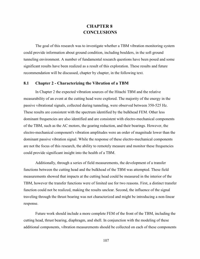
107

CHAPTER 8

CONCLUSIONS

The goal of this research was to investigate whether a TBM vibration monitoring system

could provide information about ground condition, including boulders, in the soft ground

tunneling environment. A number of fundamental research questions have been posed and some

significant results have been realized as a result of this exploration. These results and future

recommendation will be discussed, chapter by chapter, in the following text.

8.1 Chapter 2 - Characterizing the Vibration of a TBM

In Chapter 2 the expected vibration sources of the Hitachi TBM and the relative

measurability of an event at the cutting head were explored. The majority of the energy in the

passive vibrational signals, collected during tunneling, were observed between 350-525 Hz.

These results are consistent with the spectrum identified by the bulkhead FEM. Other less

dominant frequencies are also identified and are consistent with electro-mechanical components

of the TBM, such as the AC motors, the gearing reduction, and their bearings. However, the

electro-mechanical component's vibration amplitudes were an order of magnitude lower than the

dominant passive vibration signal. While the response of these electro-mechanical components

are not the focus of this research, the ability to remotely measure and monitor these frequencies

could provide significant insight into the health of a TBM.

Additionally, through a series of field measurements, the development of a transfer

functions between the cutting head and the bulkhead of the TBM was attempted. These field

measurements showed that impacts at the cutting head could be measured in the interior of the

TBM, however the transfer functions were of limited use for two reasons. First, a distinct transfer

function could not be realized, making the results unclear. Second, the influence of the signal

traveling through the thrust bearing was not characterized and might be introducing a non-linear

response.

Future work should include a more complete FEM of the front of the TBM, including the

cutting head, thrust bearing, diaphragm, and shell. In conjunction with the modeling of these

additional components, vibration measurements should be collected on each of these components

108

to better understand the coupling. In addition, a direct measurement of the input force, through

either an instrumented impact hammer or electro-dynamic shaker, should be used to generate an

impulse response measurement. This would facilitate further investigation of the transfer

function from the cutting head to the bulkhead and additional inquiries about similar responses to

the diaphragm and shell. Finally, a direct input/output measurement scheme should be employed

to more completely investigate the uncertainty regarding both measurement quality and signal

propagation. A method, like coherence testing, could be used to assist in this determination.

8.2 Chapter 3 - Boulder Detection System

In Chapter 3, the evolution of the Boulder Detection System (BDS) was developed. Three

iterations have matured into a robust measurement system. In this evolution, the BDS system has

become virtually maintenance free, autonomous, and has produced a wealth of data. The analysis

of these data sets have yielded a number of interesting results that illuminate the machine's

interaction with changes in geology. Specifically, having the ability to stitch together data sets to

produce near continuous rings of data, and then creating a stack of successive revolutions.

Further improvements of this system could include removing the small delay that is

introduced when creating a new file. A potential solution for this file delay could be employing a

double buffering mechanism during acquisition. Additionally, a system with more on-board

storage or the ability to autonomously transfer the stored data, would decrease the possibility of

over-writing files. Finally, a more expansive array of sensors should be deployed, as suggested in

the conclusion of Chapter 2.

8.3 Chapter 4 - Dynamic Characterization of TBM

In Chapter 4, operational modal analysis (OMA) is used to characterize the frequency

response of the bulkhead during operation. Specifically, frequency domain decomposition (FDD)

is explored as an OMA method. There are two main findings realized from this analysis. First,

that FDD provides a very succinct method for comparing the operational frequencies from ring

to ring. Second, there exists a strong coupling between the measured frequency response and the

rotation rate of the TBM. Results indicate that this coupling cannot be explained by traditional

forced response theory nor are the responses congruent with free vibration.

109

Future improvements should seek to develop a scale for the amplitude of the SV in the

FDD results. In addition, further research is required to understand the complex coupling

between the rotation rate and the measured frequency responses. Insight into this interaction may

come from the instrumentation of additional components and FEM, as suggested in the

conclusion of Chapter 2.

8.4 Chapter 5 - Machine Vibration and its Relationship to Ground Conditions

Chapter 5 highlights the nature of TBM vibration (in 3 dimensions) measured during the

Seattle project, its relationship to operating parameters, and its interconnections with geology

and ground conditions. TBM vibration levels varied considerably along the alignment but

showed strong correlations to changes in ground conditions, especially where there were

transitions in soil types. These findings were supported by the classical comparison of operating

parameters to changing soil conditions, yet offer additional insight into the machine/soil

interaction. Additionally, a comparison of the recorded accelerations to the Specific Energy,

which is used as a surrogate for shear strength of soil, also exhibits a strong correlation. These

discoveries offer insight into the complicated interaction between the TBM and its environment.

Future work should include alternate measurement locations, as suggested in the

conclusions of Chapter 2, and an increase in the OP data sampling rate. In addition, a less

complicated geologic alignment and a more comprehensive geological profile could help to de-

couple the complex interaction between the TBM and its vibratory response. Finally, the FDD

methods, discussed in Chapter 4, might offer a more succinct comparison between the vibratory

response of the TBM and classified geology.

8.5 Chapter 6 - Principal Motion

In Chapter 6, a filtering process called principal motion (PM) was explored. This

approach provides a mechanism to separate the flexible motion from the rigid body motion in a

grouped set of measurements. Simulation results of PM illustrate that this method can provide

insight into the rigid body response of the TBM. However, as the simulations and the application

of PM to field data show, the calculations are sensitive to measurement noise and interpretation

of these results is challenging. In addition, as discussed in Chapter 2, the response could be the

110

local bulkhead's modal response (mode 1 of Figure 2.7) and not the response of the entire TBM

(rigid body motion), as desired.

An extension of this work could look at adding additional sensors, near the peripheral of

the shield, to potentially address the local response uncertainty.

8.6 Chapter 7 - University-Industry Collaboration in the Underground

Construction And Tunneling Field

There are several barriers and opportunities affecting prospects for increasing

collaboration between academia and industry in the field of UC&T. Several of these barriers are

institutional, such as the low number of universities offering programs that support the UC&T

field or the diminishing federal and municipal budgets. However, the majority of the hurdles are

a result of dissimilar short term goals. In many cases, the long term goals are well aligned, but

the frameworks are not in place to support collaboration. As this research has shown, there are

several opportunities to bridge this gap through internships and collaborative research projects.

111

REFERENCES CITED

[1] B. Maidl, M. Herrenknecht, U. Maidl, and G. Wehrmeyer, Mechanised Shield Tunnelling,

2nd ed. Wilhelm Ernst & Sohn, 2012, p. 470.

[2] R. Teale, “The concept of specific energy in rock drilling,” International Journal of Rock

Mechanics and Mining, vol. 2, no. July 1964, pp. 57–73, 1965.

[3] B. Celada, J. Galera, C. Muñoz, and I. Tardáguila, “The use of the Specific Drilling

Energy for Rock Mass Characterisation and TBM Driving During Tunnel Construction,”

in ITA-AITES World Tunnel Congress, 2009, pp. 1–13.

[4] G. A. Cooper, M. Lesage, M. Sheppard, and P. Wand, “The interpretation of tricone drill

bit vibrations for bit wear and rock type,” in Proc. Rapid Excavation and Tunneling

Conference, June, 1987, pp. 14–18.

[5] G. Heisig, J. Sancho, and J. D. Macpherson, “Downhole Diagnosis of Drilling Dynamics

Data Provides New Level Drilling Process Control to Driller,” in SPE Annual Technical

Conference, 1998, pp. 649–658.

[6] O. J. Hoffmann, J. R. Jain, R. W. Spencer, and N. Makkar, “Drilling dynamics

measurements at the drill bit to address today’s challenges,” in Instrumentation and

Measurement Technology Conference (I2MTC), 2012 IEEE International, 2012, pp. 443–

448.

[7] D. J. Ewins, Modal Testing: Theory, Practice and Application, 2nd ed. Research Studies

Press Ltd, 2000, p. 562.

[8] R. Brincker, L. Zhang, and P. Andersen, “Modal Identification from Ambient Response

using Frequency Domain Decomposition,” in 18th International Modal Analysis

Conference, 2000, p. 11.

[9] J. S. Bendat and A. Piersol, Engineering Applications of Correlation and Spectral

Analysis, 2nd ed. John Wiley & Sons, Inc, 1993, p. 458.

[10] “LabVIEW - Sound and Vibration Measurement Suite.” National Instruments, Austin,

2011.

[11] R. Barron, Ed., Engineering Condition Monitoring Practice, methods and applications.

Addison Wesley Longman, Inc, 1996, p. 239.

[12] K. Baker, “Singular Value Decomposition Tutorial,” 2013. [Online]. Available:

http://www.ling.ohio-

state.edu/~kbaker/pubs/Singular_Value_Decomposition_Tutorial.pdf.

112

[13] M. A. Diponio, G. Frank, E. A. Gharahbagh, and E. Cording, “Settlement Risk of

Extended Overcut in Dense Soils,” in North American Tunneling 2012, 2012, pp. 54–64.

[14] R. J. Irish, “Pre-Bid Engineering Geologic Evaluation of Subsurface Conditions for the

University Link Light Rail Tunnels, Capitol Hill Station to Pine Street Stub Tunnel, and

Capitol Hill Station Excavation and Supprt, Contract U230 Seattle, Washington,” 2009.

[15] P. J. Tarkoy, “Challenges & Successes in Micro-Tunneling on the Chelsea River

Crossing,” in 5th International Microtunnelling Symposium, 2001, no. April, pp. 1–16.

[16] T. Cunningham and D. Hensley, “Using IMAT and MATLAB for coriolis flowmeter

design.,” in IMAC-XIX, 2001, pp. 1–7.

[17] D. Hensley and T. Cunningham, “Principal Motion,” 2012.

[18] “Tunnel Education at the Mile High Level,” Trenchless Technology, pp. 11–12, Nov-

2010.

[19] “Long Island Rail Road East Side Access,” Metropolitan Transportation Authority, 2013.

[Online]. Available: http://www.mta.info/capconstr/esas/. [Accessed: 07-Sep-2013].

[20] “Tunnel and Reservoir Plan (TARP),” Metropolitan Water Reclamation District of

Greater Chicago, 2013. [Online]. Available:

http://www.mwrd.org/irj/portal/anonymous/tarp. [Accessed: 07-Sep-2013].

[21] “Alaskan Way Viaduct Replacement Program,” Transportation, Washington State

Department of, 2013. [Online]. Available: http://www.wsdot.wa.gov/projects/Viaduct/.

[22] G. Brierley and A. Hawks, “Tunnel education in the United States,” Tunneling &

Underground Construction, no. June, pp. 18–21, 2010.

[23] P. Asadollahi and A. Zeytinci, “Sustainable development of infrastructures using

underground spaces: role of academia,” ASEE Middle Atlantic Regional Conference, no.

Figure 1, 2011.

[24] J. K. Lemley, “Towards New Worlds in Tunneling: Advancing the ‘Art of the Possible’,”

Tunnelling and Underground Space Technology, vol. 8, no. 1, pp. 3–6, Jan. 1993.

[25] M. K. McCarter, “Mining faculty in the United States : current status and sustainability,”

Mining Engineering, no. SEptEMbEr, pp. 28–33, 2007.

[26] D. O. Gray, L. Tornatzky, L. McGowen, and E. Sundrome, “Research Center

Sustainability and Survival: Case Studies of Fidelity, Reinvention and Leadership of

Industry/University Cooperative Research Centers,” 2012.

113

[27] NSF, “Industry & University Cooperative Research Program (I/UCRC),” 2013. [Online].

Available: http://www.nsf.gov/eng/iip/iucrc/.

[28] D. O. Gray, “Making Team Science Better: Applying Improvement-Oriented Evaluation

Principles to Evaluation of Cooperative Research Centers,” New Directions for

Evaluation, no. 118, pp. 73–87, 2008.

[29] D. Gray, E. Sundstrom, L. G. Tornatzky, and L. McGowen, “When Triple Helix unravels:

A multi-case analysis of failures in industry–university cooperative research centres,”

Industry and Higher Education, vol. 25, no. 5, pp. 333–345, Oct. 2011.

[30] E. P. Berman, Creating the Market University:How Academic Science Became an

Economic Engine. Princeton University Press, 2012, p. 265.

[31] J. Washburn, University Inc.:The Corporate Corruption of Higher Education. Basic

Books, 2005, p. 328.

[32] G. West, Innovation and the rise of the tunnelling industry. Press Syndicate of the

University of Cambridge, 1988, p. 355.

[33] “SME Student Scholarships,” Society for Mining, Metallurgy and Exploration (SME),

2013. [Online]. Available: http://www.smenet.org/scholarships/.

[34] SME, “RETC History: Attendance & Exhibitor Stats,” 2013. [Online]. Available:

http://www.retc.org/stats.cfm.

[35] M. A. Diponio and C. Dixon, “2013 Proceedings,” in RETC Proceededings, 2013, p.

1350.

[36] “Pilot Tube Microtunneling/Microtunneling Short Course,” Colorado School of Mines,

2013. [Online]. Available: http://csmspace.com/events/microtunnel/.

[37] S. Wallis and J. Green, “Technical delivery at RETC,” Tunnel Talk, 2013. [Online].

Available: http://tunneltalk.com/RETC2013-roundup-27June2013-A-focus-on-

technology-and-development.php.

[38] E. A. Gharahbagh, J. Rostami, K. Talebi, and J. Ibarra, “EXPERIMENTAL STUDY OF

IMPACT OF SOIL CONDITIONING ON SOIL ABRASION AND CUTTER,” in Rapid

Excavation and Tunneling Conference 2013 Proceedings, 2013, pp. 1052–1064.

[39] M. A. Diponio, J. Dee, B. Hagan, P. Raleigh, and J. Associates, “KEEPING THE

CHAMBER FULL : MANAGING THE ‘ AIR BUBBLE ’ IN EPB TUNNELING,” in

Rapid Excavation and Tunneling Conference 2013 Proceedings, 2013, pp. 1065–1073.

114

[40] M. M. Shinouda and J. Dee, “UNTANGLING THE MYSTERY OF SOIL

CONDITIONING,” in Rapid Excavation and Tunneling Conference 2013 Proceedings,

2013, pp. 1074–1085.

[41] Anonymous, “Schooling in earth systems,” T&T North America, p. 14, 2000.

[42] Colorado School of Mines, “Alumnus Gives $5 million to Underground Construction and

Tunneling Program, Scholarships,” Giving News, 2012. [Online]. Available:

http://giving.mines.edu/s/840/giveindex.aspx?sid=840&gid=1&pgid=2271.

[43] “2013 Tunneling Industry Forecast,” Tunnel Business Magazine, 2013. [Online].

Available: http://www.tunnelingonline.com/2013-tunneling-industry-orecast/. [Accessed:

10-Jan-2013].

[44] P. Norvig and S. J. Russel, Eds., Artificial Intelligence: A Modern Approach, 3rd ed.

Prentice Hall, 2010, p. 1132.

[45] M. H. Beale, M. T. Hagan, and H. B. Demuth, “Neural Network Toolbox TM

User ’ s

Guide,” Natick, 2013.

[46] J. Hollmen, “Self-Organizing Map (SOM),” 1996. [Online]. Available:

http://users.ics.aalto.fi/jhollmen/dippa/node9.html. [Accessed: 08-Jun-2013].

[47] “KNIME.” KNIME.com AG, Zurich, 2013.

[48] F. Berthold, M.R., Borgelt, C., Höppner, F., Klawonn, Guide to Intelligent Data Analysis.

Springer, 2010, p. 394.

[49] “Links to Mining Schools,” Mine Safety and Health Administration, 2013. [Online].

Available: http://www.msha.gov/SITEINF2.HTM. [Accessed: 07-Dec-2013].

[50] “List of Mining Schools,” Everything Mining, 2013. [Online]. Available:

http://www.everythingmining.com/list_of_mining_schools.htm. [Accessed: 07-Dec-

2013].

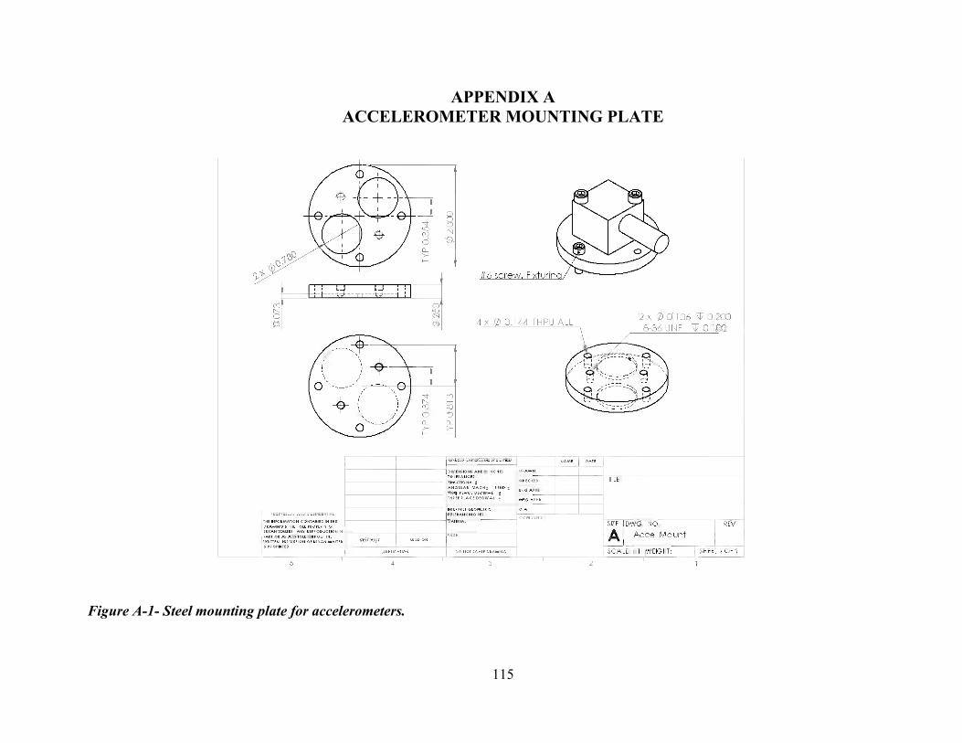
115

APPENDIX A

ACCELEROMETER MOUNTING PLATE

Figure A-1- Steel mounting plate for accelerometers.

116

APPENDIX B

TAP TEST NOISE FLOOR

Figure B-1- Estimate of DAQ noise floor (a) FFT of the accelerometer mounted to the cutting

head (b) FFT of the accelerometers mounted to the bulkhead of the TBM. The amplitude scale

is in dB with a 1g-reference amplitude.

117

APPENDIX C

TRANSMISSIBILITY RESULTS OF PRELIMINARY

BULKHEAD MEASUREMENTS

Figure C-1- Transfer function estimates for striking position 0 on the TBM's cutting head. (a)

Shows the response of accelerometers a2, a3 and a4 in the transverse direction. (b) Shows the

response of accelerometers a2, a3 and a4 in the vertical direction. (c) Shows the response of

accelerometers a2, a3 and a4 in the longitudinal direction. The amplitude scale is in dB with a

1g-reference amplitude.

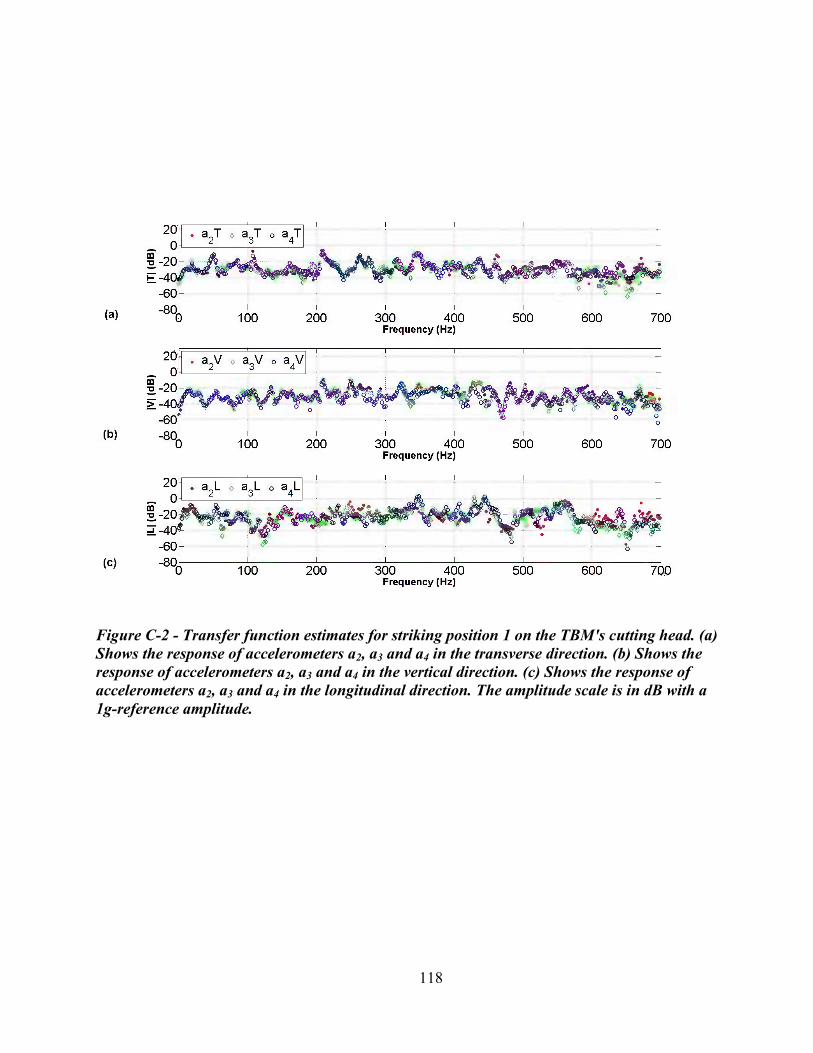
118

Figure C-2 - Transfer function estimates for striking position 1 on the TBM's cutting head. (a)





119

Figure C-3 - Transfer function estimates for striking position 2 on the TBM's cutting head. (a)





120






121






122






123






124






125

APPENDIX D

BDS #1 SENSOR CALIBRATION INFORMATION

The following graphs show the calibration of the accelerometers with respect to the

earth’s gravitational field. These values are consistent with the manufactures stated sensitivity of

100mV/g. For a complete reference, please see Analog Devices datasheet for the ADXL321

MEMs type accelerometer.

Figure D-1 - Calibration for transverse axis 1

Figure D-2- Calibration for transverse axis 2

126

Figure D-3- Calibration for longitudinal axis

Figure D-4- Calibration for the vertical axis

127

APPENDIX E

STITCHING SUCCESIVE FILES TOGETHER

function [padded_data] = zero_pad_stiched_Ring_data_fcn(data)

fs = 2000; % Hz

[row,col] = size(data);

num_samples = row; file_size = 160000;

theo_num_elements = ceil(data(end,1)*fs);

t_padded = 0:1/fs:data(end,1); padded_data = zeros(theo_num_elements,13);

num_files = num_samples/file_size;

%% aa=1; bb=file_size;

cc=1; dd=file_size;

for i=1:num_files-1

if bb >= num_samples bb = num_samples; dd = theo_num_elements; offset = 0; else offset = ceil((data(bb+1,1)-data(bb,1))*fs); end

padded_data(cc:dd,2:13) = data(aa:bb,2:13);

aa = bb + 1; bb = bb + file_size;

cc = dd + offset + 1; dd = dd + offset + file_size;

end

padded_data(theo_num_elements-file_size:theo_num_elements,2:13) = data(row-

file_size:row,2:13);

padded_data(:,1) = t_padded(1:theo_num_elements);

128

APPENDIX F

MACHINE LEARNING/PATTERN RECOGNITION

Machine learning was used to investigate the relationship between vibration

measurements, machine operating parameters, and different soil conditions. The goal of using

machine learning was to examine the hypothesis that a passive vibration system is sensitive to

geologic changes. Within the scope of this research, machine learning was used as a tool to

classify the TBM monitoring data by both un-supervised and supervised learning methods.

F.1 Unsupervised Learning

In unsupervised learning the goal is to recognize patterns in the data without explicit

feedback [44]. In this research there are two groups of data, the TBM's OP data and the vibration

data. As discussed in Section 3.4, the OP data contains machine parameters such as Advance

Rate (AR), Torque (T), Rotation Rate (N), EPB plenum pressure (σ) and Force (F). The vibration

data contains RMS amplitudes for the four triaxial accelerometers in the three principal

directions, transverse (T), vertical (V), and longitudinal (L). A portion of these two data sets is

show graphically in Figure .

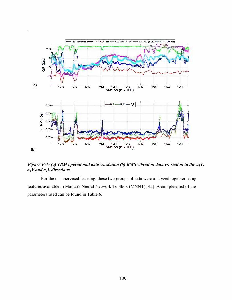
129

.

Figure F-1- (a) TBM operational data vs. station (b) RMS vibration data vs. station in the a1T,

a1V and a1L directions.

For the unsupervised learning, these two groups of data were analyzed together using

features available in Matlab's Neural Network Toolbox (MNNT).[45] A complete list of the

parameters used can be found in Table 6.

130

Table 6 - Parameters used for unsupervised learning

# Parameter Units

1 Cutting Head Rotation Rate RPM

2 Cutting Head Power kW

3 EPB Plenum Pressure Bar

4 Thrust Force kN

5 Advance Rate Mm/min

6 Cutting Head Torque kN-m

7 a1T g

8 a1V g

9 a1L g

10 a2T g

11 a2V g

12 a2L g

13 a3T g

14 a3V g

15 a3L g

16 a4T g

17 a4V g

18 a4L g

One method of unsupervised learning that has been successfully used to characterize

data, without requiring a probabilistic understanding of the input/output relationship, is the self-

organizing map (SOM). The SOM is a tool that can be used to visualize high-dimensional data

by mapping the data onto a plane [46]. One example of this visualization can be seen in Figure ,

where the input data, eighteen parameters collected over 368 rings, are mapped to grids called

neurons and shown as grey dots. In Figure , there are four iterations of grid size, where the grid is

increased in powers of 2, from 4 to 32. This progression was done to visually evaluate if and

when the data is forming clusters. These visualization were generated with MNNT's function

SOM Neighbor Distances (plotsomnd). The connections or distances between the neurons are

color coded to show their direct relationship to their neighbor, the scale goes from yellow to

black, where yellow indicates the closest relationship. Typically, when a relationship or cluster is

131

found in the data it can be visually seen by the collection of similar colors grouped together.

Figure does not exhibit this clustering, indicating that there is not a distinct relationship detected

between these parameters.

Figure F-2- Results of SOM cluster nearest neighbor distances with (a) a 4x4 topology, (b) a

8x8 topology, (c) a 16x16topology , and (d) a 32x32 topology.

Additionally, the weights that characterize the connection of each of the eighteen input

parameter to a neuron can be visualized independently. Using MNNT's function Plot SOM

weight planes (plotsomplanes), a visual representation is produced. Figure shows these results,

where lighter colors (yellow) indicate large weights and darker colors (black) indicate a smaller

weight. Similar patterns are an indication of high correlation, which is apparent in inputs 7-18,

the twelve accelerometer measurements. Input 4, which is the thrust measurements, appear to

have several distinct regions, indicating that there is some level of classification associated with

this input.

132

Figure F-3- Results of the neuron weights for each of the eighteen inputs, where each input is

shown in (a) a 4x4 topology, (b) a 8x8 topology, (c) a 16x16topology , and (d) a 32x32

topology.

Another plot that can help to visualize the number of data points affiliated with each

neuron is the SOM Sample Hits tool (plotsomhits), available in MNNT. A visual representation

of the data listed in Table 6 can be seen in Figure , where the relative size of the grey hexagons

indicate the number of data points associated with each neuron. As suggested in MNNT's users

guide, the data would ideally be evenly distributed amongst the neurons. Figure (b)-(d) shows

that the data is peppered throughout the neurons and therefore not evenly distributed.

133

Figure F-4- Results of the relative number of data points affiliated with each neuron for (a) a

4x4 topology, (b) a 8x8 topology, (c) a 16x16topology , and (d) a 32x32 topology.

Yet another visualization tool is the plot SOM Weight Positions (plotsompos), also

available in MNNT. Figure shows a visualization of the classification of the input domain,

where the input vector is represented by green dots and the neuron's weight position is indicated

by blue-grey dots. The OP and vibration data from the Seattle project produced the results shown

in Figure (a), which are very linearly condensed. In comparison to MNNT's example data set,

shown in Figure (b), the results for the OP and vibration data indicate that there is not much

separation between the input vector and the weights of the neuron.

134

Figure F-5- Spatial representation of the neuron's weight positions for (a) the Seattle OP and

vibration data, and (b) an example data set.

F.2 Supervised Learning

In supervised learning, patterns in the data are developed from a defined input-output

relationship, where these relationships are used to train algorithm that classify a series of

data.[44] In this research, the OP and vibration values, recorded in known geologies, are used to

characterize the input-output relationship. Figure shows a cross section of the tunnel alignment

overlaid with the geological profile. In addition, Figure , also indicated the location of eight

borings, where the soil was extracted and classified. These eight regions, plus an additional two

that were chosen to evaluate similar soils where borings were not taken, are combined to form

ten classes. The class identifiers and their position can be seen along the bottom of Figure .

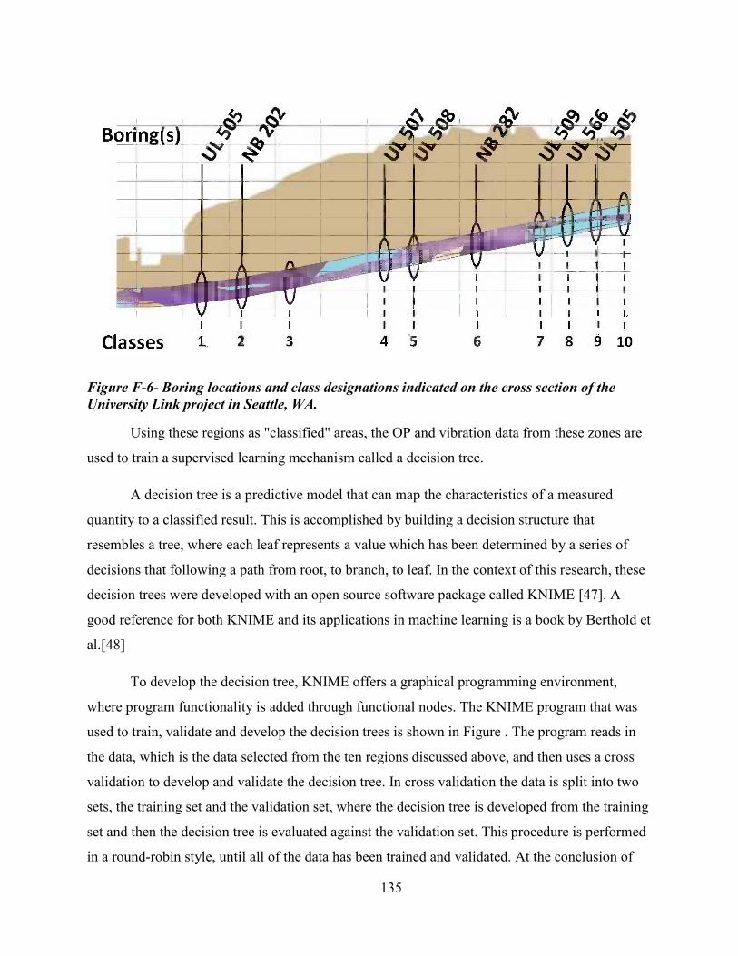
135

Figure F-6- Boring locations and class designations indicated on the cross section of the

University Link project in Seattle, WA.

Using these regions as "classified" areas, the OP and vibration data from these zones are

used to train a supervised learning mechanism called a decision tree.

A decision tree is a predictive model that can map the characteristics of a measured

quantity to a classified result. This is accomplished by building a decision structure that

resembles a tree, where each leaf represents a value which has been determined by a series of

decisions that following a path from root, to branch, to leaf. In the context of this research, these

decision trees were developed with an open source software package called KNIME [47]. A

good reference for both KNIME and its applications in machine learning is a book by Berthold et

al.[48]

To develop the decision tree, KNIME offers a graphical programming environment,

where program functionality is added through functional nodes. The KNIME program that was

used to train, validate and develop the decision trees is shown in Figure . The program reads in

the data, which is the data selected from the ten regions discussed above, and then uses a cross

validation to develop and validate the decision tree. In cross validation the data is split into two

sets, the training set and the validation set, where the decision tree is developed from the training

set and then the decision tree is evaluated against the validation set. This procedure is performed

in a round-robin style, until all of the data has been trained and validated. At the conclusion of

136

the training, the overall accuracy of the model can be reviewed. The overall accuracy is an

averaged value that quantifies how well the decision tree, that was developed from the validation

training sets, were able to correctly classify the training set. Therefore, a value of 85% overall

accuracy indicates that the decision tree's application on the validation data, correctly classified

the data 85% of the time.

Figure F-7- Graphical program used to train, validate and develop the decision tree.

To investigate the correlation between the OP and vibration data and the geology, the

following three combinations of the data sets were evaluated: 1) the combination of the OP and

vibration data, 2) OP data only and 3) the vibration data only. To more clearly explain a decision

tree and its use, a graphical representation of a decision tree is shown in Figure . The decision

tree provides a map for the classification of each data set, where a data set consists of the

eighteen parameters identified in Table 6, into a distinct class. For example, using Figure , if the

EPB pressure was greater than 1.79 bar and the rotation rate was greater than 2.0 rpm, then the

decision tree would codify the data set as belonging to Class 10.

137

Figure F-8- Graphic representation of a decision tree, where each leaf (shown in red)

indicates the codification of the data set.

Using both the OP and vibration data to train and develop a decision tree produces a

visually complicated decision tree, as shown in Figure . Nevertheless, by apply the simple

greater than less than rules of the decision tree a data set can be boiled down to a unique class.

As can be seen in Figure , the top discriminating parameter are the EPB pressure, followed by

rotation rate. The overall accuracy reported for the OP and vibration decision tree was 89%.

Next just the OP data was used to classify the geology. This increased the overall

accuracy from 89% to 91%. The two most discriminating parameters, once again, are the EPB

Pressure and rotation rate, as can be seen in Figure .

138

Figure F-9- Graphic representation of the decision tree obtained from using KNIME to

identify the correlations between OP and vibration data and soil type.


identify the correlations between OP and soil type.

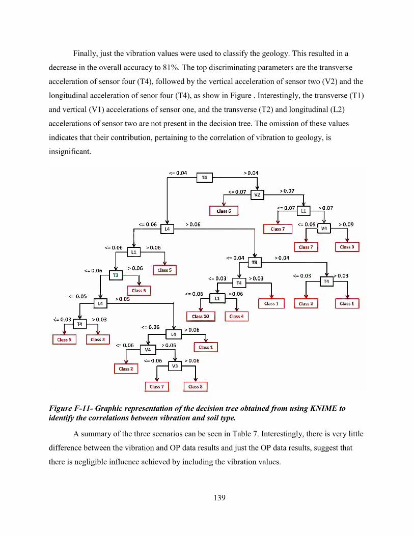
139

Finally, just the vibration values were used to classify the geology. This resulted in a

decrease in the overall accuracy to 81%. The top discriminating parameters are the transverse

acceleration of sensor four (T4), followed by the vertical acceleration of sensor two (V2) and the

longitudinal acceleration of senor four (T4), as show in Figure . Interestingly, the transverse (T1)

and vertical (V1) accelerations of sensor one, and the transverse (T2) and longitudinal (L2)

accelerations of sensor two are not present in the decision tree. The omission of these values

indicates that their contribution, pertaining to the correlation of vibration to geology, is

insignificant.


identify the correlations between vibration and soil type.

A summary of the three scenarios can be seen in Table 7. Interestingly, there is very little

difference between the vibration and OP data results and just the OP data results, suggest that

there is negligible influence achieved by including the vibration values.

140

Table 7 - Summary of Decision Tree Results

Data Set Description Overall Accuracy

Vibration and OP Data 89%

OP Data only 91%

Vibration Data only 81%

Nevertheless, since the objective of this research is to find correlation with passive

vibration measurements, the decision tree developed from both the vibration and OP data will be

used to evaluated the entire data. The results are shown near the bottom of Figure , where the ten

uniquely colored diamonds indicate the "trained" values, and the smaller colored dots are the

results of the decision tree applied to the entire data set. As expected, the colors of the small dots

inside the large diamonds are the same color. However, in many of the areas adjacent to the

diamonds, the color deviates. For example, around Class 6, the majority of the small dots are red,

the color associated with Class 10. This indicates that the decision tree is not able to discriminate

between these two values. On the other hand, there are other regions where the correlation looks

positive, especially near Classes 1 and Class 7.

Figure F-12- Results of the ten class decision tree obtained by applying the algorithm to the

entire set of data.

F. 3 Summary of Machine Learning Results

141

The results of using machine learning to correlate geology with the OP and vibration data

presented here illustrate several outcomes. First, for the unsupervised learning, the results

indicate that there is no significant clustering of the OP and vibration data sets. This suggests that

the parameters chosen for this analysis do not vary with changes in geology. Second, for the

supervised learning, the results indicate several useful findings: 1) that EPB Pressure and rotation

rate are the strongest indicator of geology type, 2) that sensors three and four, offer the greatest

capacity for estimating relations between geology and vibration, especially in the vertical and

longitudinal directions and, 3) that including the RMS vibration value offers little improvements

over using just the OP data for distinguishing geologic changes.

142

Appendix A UC&T SCHOOLS

Table 8 - UC&T Schools

University Phone Courses or Other Supporting Information Colorado School of Mines

Undergraduate Minor, graduate degrees

Cornell

(607) 254-4636 Professor O'Rourke, underground technologies

Idaho State

(208) 282-2902 CE 4454 Basic Engineering Geology

Indiana University-Purdue

University Indianapolis

(317) 274-2533

Graduate Course, Strategic Asset Management for Infrastructure &

Trenchless Technology

Louisiana Tech

(318) 257-2260

Trenchless Technology Center, 480: Introduction to Trenchless Technology,

580: Trenchless Technology

Massachusetts Institute of

Technology

1.383 Underground Construction

Missouri University of Science and

Technology

(800) 522-0938

371 Rock Engineering, Min Eng 383 (Tunneling & Underground

Construction Techniques)

[22][49][50]

143

Table 8 - UC&T Schools (Continued)

University Phone Courses or Other Supporting Information Montana Tech of the

University of

Montana (800) 445-8324

New Jersey Institute

of Technology

(973) 596-5534 CE 614 Underground Construction

New Mexico Institute

of Mining and

Technology

(575) 835-5500

ME 434, Drilling and Blasting Engineering,ME 442, Applied Geomechanics, ME 534,

Advanced Drilling and Blasting Engineering, ME 537, Design and Construction of

Underground, ME 540, Computer Application in Geotechnical

Engineering

Pennsylvania State

(814) 865-6546

Purdue University

(765) 494 - 2166 CE 686: Underground Construction

South Dakota School

of Mines and

Technology (605) 394-2439

MEM 303 Underground Mining Methods and Equipment, MEM 305 Introduction to

Explosives Engineering, MEM 415/515 Advanced Mining Geotechnical Engineering,

MEM 420/520 Advanced Tunneling and Underground Excavation

Southern Illinois

University at

Carbondale (618) 453-2963 321-3 Underground Mining, 475-3 Analysis and Design of Mine Excavations

University of Arizona

(520) 621-6594

MNE 447 - Underground Construction Geomechanics, MNE 547 - Underground

Construction Geomechanics,

University of Illinois

at Urbana-Champaign

217/333-2151 CEE 480 Foundation Engineering, CEE 588 Geotechnical Earthquake Engrg

144

Table 8 - UC&T Schools (Continued)

University Phone Courses or Other Supporting Information University of Kentucky

859-257-8026 talked to faculty, there is a course called Underground Construction

University of

Minnesota

612-624-2006

CE 4426 - Rock Mechanics, CE 4436 - Design of Underground and Surface Excavations

in Rock, CE 5426 - Rock Mechanics , CE 5436 - Design of Underground and Surface

Excavations in Rock

University of Nevada

Reno's Mackay School

of Mines (775) 784-4591

GE 740 Design of Surface and Underground Excavations, MINE 458 Rock Mechanics

for Underground Mining and Construction, MINE 658 Rock Mechanics for Underground

Mining and Construction

University of Texas at

Austin

512-471-7995 Certificate

Documents

detecting changing geologic conditions with tunnel boring machines