Embed Size (px)
Citation preview

REVSTAT – Statistical Journal
Volume 7, Number 1, April 2009, 67–85
DETECTING SOCIAL INTERACTIONS IN BIVARI-
ATE PROBIT MODELS WITH AN ENDOGENOUS
DUMMY VARIABLE: SOME SIMULATION RESULTS
Author: Johannes Jaenicke
– Faculty of Economics, Law and Social Sciences,University of Erfurt, [email protected]
Abstract:
• This paper analyzes the possibility of detecting observable and non-observable socialinteractions in a bivariate probit model with an endogenous dummy regressor viaMonte Carlo simulation. In small samples, we find severe size distortions of theWald test and only a low probability of detecting observable and non-observablesocial interactions. In large samples, however, we find this test to be very powerful.
Key-Words:
• parameter tests; bivariate probit model; Monte Carlo study.
AMS Subject Classification:
• 62F03, 62P20.

68 Johannes Jaenicke

Detecting Social Interactions in Bivariate Probit Models 69
1. INTRODUCTION
For the researcher, interactions between two persons, e.g., spouses or
brothers and sisters may only partly be observable, due to measurement
problems. Respondents may not wish to reveal the influence of the other person
or may not be aware of them. In order to detect the neglected or non-observable
interactions between the respective decision processes a bivariate probit model
is recommendable (Jaenicke, 2004).
The identification of discrete choice models with social interactions is stud-
ied by Brock and Durlauf (2001, 2007). They show that it is possible to overcome
Manski’s (1993) famous reflection problem discussed in the context of reference
group behaviour by using discrete choice models. In order to account for the ne-
glected or non-observable interactions between discrete decisions in the respective
decision processes, a bivariate probit model is a useful empirical description of
this process. In this model, an endogenous dummy variable represents the binary
decision of the peer that may have an influence on the second person. The bivari-
ate probit model with an endogenous dummy variable is introduced by Maddala
and Lee (1976) and belongs to a general class of simultaneous equation models
discussed by Heckmann (1978), Maddala (1983), Wilde (2000, 2004), and Greene
(2008).
In some applications of the bivariate probit model, e.g. Dean (1995), and
Greene (1998) only small samples with 76 or 132 observations are available.
However, even in data sets with 500, 1,000 or 2,000 observations, parameter
tests may be crucial, as shown by Monfardini and Radici (2008).
Our intention is to find out for different sample sizes whether, in the pres-
ence of social interactions, it is possible to detect these interactions in a bivariate
probit model with an endogenous dummy regressor. Hence we analyze the distri-
bution of the estimated parameters and size and power of the usual z-coefficient
test concerning the parameters of the observable and non-observable interactions,
i.e. the endogenous dummy variable and the residual covariance between both
equations of this bivariate probit model.
2. A BIVARIATE PROBIT MODEL OF SOCIAL INTERACTIONS
The maximum likelihood estimation of a bivariate probit model involves
the numerical problem of the evaluation of double integrals over the normal dis-
tribution. This estimation procedure is implemented in several statistic software
packages and widely used in practice. We use a two equation binary choice model
with an endogenous dummy regressor, first proposed by Maddala and Lee (1976).

70 Johannes Jaenicke
The regression equations of the individual I and the peer P are
Y ∗
I = XI β1 + YP β2 + uI , YI = 1 if Y ∗
I > 0, 0 otherwise ,
Y ∗
P = XP γ1 + uP , YP = 1 if Y ∗
P > 0, 0 otherwise ,
[uI , uP ] ∼ Φ2(0, 0, 1, 1, ρ) ,
with the observable discrete choice behavior Y , latent variables Y ∗
I , and exoge-
nous variables X. The residual vector [uI , uP ] is bivariate normal distributed
with E(ui) = 0, var(ui) = 1, i = I, P , and cov(uI , uP ) = ρ. As a condition of
identification, we only need exclusion restrictions if there is no variation of the
exogenous regressors (Wilde, 2000).
In our model, the observable part of the social interactions, the influence
of the decision of the peer P on the behavior of the individual I is tested by
the hypothesis H0 : β2 = 0. The non-observable part of the social interactions
may be revealed through the residual covariance structure. A residual covariance
cov(uI , uP ), i.e. ρ, significantly different from zero, may serve as an indicator of
unobserved social interactions between the two decisions or as an indicator of si-
multaneously neglected third-party effects. Restricting residual correlation of the
bivariate probit model to zero may result in biased and inconsistent estimations
(Murphy, 1995). Fitting separate probit models for the first- and the second
decision equation can involve significant endogeneity biases in the estimation
(Lollivier, 2001). The joint estimation of the two equations provides substantial
efficiency gains compared to separate estimation based on two-stage technique.
3. MONTE CARLO RESULTS FOR THE BIVARIATE PROBIT
MODEL
In a small Monte Carlo study, we analyze the size and the power of the
usual z-coefficient tests concerning the parameters of the observable and non-
observable social interactions, β2 and ρ. The test statistics are z(β2) = β2/se(β2)
and z(ρ) = ρ/se(ρ) and their squares result in the standard Wald test (Greene
2008, p. 820).
The non-observable influences stem from missing variables. These may
be uncorrelated, weakly or strongly correlated or identically for the two per-
sons. To create the non-observable interactions, we use an omitted variable vec-
tor [vI , vP ] ∼ Φ2(0, 0, 1, 1, r) with r ∈ [0.0, 0.1, 0.2, 0.3, 0.4, 0.5, 1.0] in one set of
experiments. In this case, the residuals ui, i = I, P , are the sum ui = vi + εi
with [εI , εP ] ∼ Φ2(0, 0, 1, 1, 0), therefore [uI , uP ] ∼ Φ2(0, 0, 2, 2, r2). Because the
assumption of the unit residual variance var(ui) is not met, we expect some prob-
lems resulting from the misspecification of the model.

Detecting Social Interactions in Bivariate Probit Models 71
In the experiments with the extended model, we include vi as additional
explanatory variables. In this case, the residuals are ui = εi and are independent
normal distributed. Because of the independence of the residuals, ρ = 0, the
model is overparametrized. Two single equation models would be more efficient.
Anyway, since we do not know the true parameter set in the empirical research
situation, in the simulation experiments we continue with bivariate probit models.
The variables Xi, i = I, P , are standard normal distributed, Xi ∼ N(0, 1),
i = I, P . All parameters β and γ in the omitted variable model and in the ex-
tended model are set equal to one. We use the econometric software package
Limdep 7.0. It performs well in nonlinear estimation benchmark tests (Mc-
Cullough, 1999). We estimate the bivariate models with the default settings
of the procedure (algorithm: BFGS; maximum iterations: 100). The Broyden–
Fletcher–Goldfarb–Shanno (BFGS) algorithm is rather time consuming, but it
shows a convergence rate of between 99.5 percent (in small data sets with 100
observations) and 100 percent (in data sets with 10,000 observations) in our
Monte Carlo study. The number of replications in the Monte Carlo experiment
is N = 1,000. The number of observations varies systematically from T = 100
to T = 2,000. In some experiments, we estimate data sets up to T = 10,000 and
in one up to T = 40,000 observations. Due to the nonlinear estimation problem,
experiments with these huge data sets are computational intensive, e.g., some
experiments need around 84 hours on a Pentium(R), 3.2GHz to estimate two
bivariate probit models 1,000 times.
The estimated parameters ρ show no severe bias. Figure 1 presents the
density estimation with the Epanechnikov kernel function in the case that the
true parameter ρ = 0. With increasing sample size from T = 200 to T = 1,000,
0.0
0.4
0.8
1.2
1.6
2.0
2.4
2.8
3.2
-1.00 -0.75 -0.50 -0.25 0.00 0.25 0.50 0.75 1.00
200 obs 500 obs 1000 obs
De
nsity
Figure 1: Kernel estimation, rho=0
rho
Figure 1: Kernel estimation, ρ = 0.

72 Johannes Jaenicke
the dispersion of the estimated parameters becomes smaller. The parameters
are distributed more or less symmetrically (with skewness ST between −0.083
and −0.040) and means (with ρT between −0.001 and 0.003) very close to the
theoretical value zero.
The picture changes if we assume with ρ = 0.5 strong residual correlation
between both decision equations in small data sets. In the case of T = 200,
we find with ρ200 = 0.485 some deviations from the theoretical parameter value.
In all three cases, the distribution of the estimated parameters ρ200 is left skewed
with a skewness ST between −0.568 and −0.403. In the T = 200 case, some ρ200
are very close the theoretical limit of 1. In Figure 2, we present a Kernel density
estimation for ρ = 0.5 and T = 200, T = 500 and T = 1,000.
0
1
2
3
4
-1.00 -0.75 -0.50 -0.25 0.00 0.25 0.50 0.75 1.00
200 obs 500 obs 1000 obs
De
nsity
rho
Figure 2: Kernel estimation, rho=0.5
Figure 2: Kernel estimation, ρ = 0.5.
Looking at the z-statistics in the case ρ = 0, we find some indication
that the z-statistics may not be normally distributed in small samples. To ana-
lyze this problem graphically, we compare the quantiles of these statistics with
the standard normal distribution in Figure 3 for T = 200, 500, 1000 observations.
Especially in the case of ρ = 0, T = 200 observations, we find some deviation from
normality.
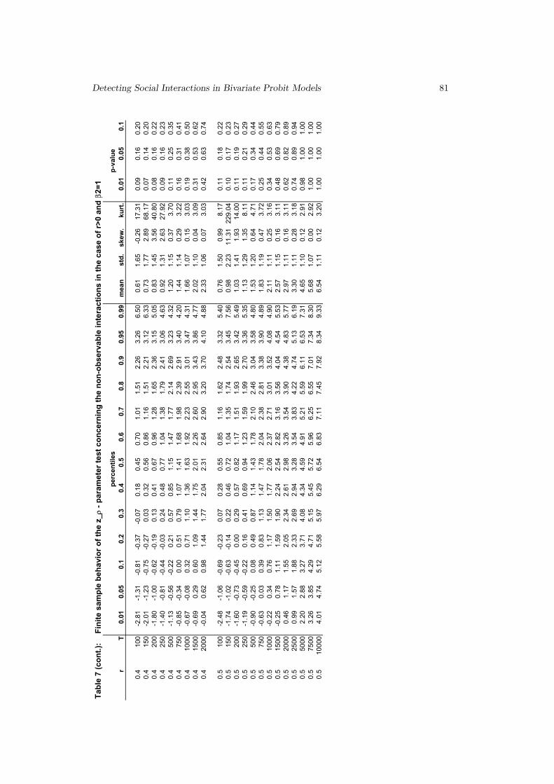
We start our analysis studying possible size distortions of the zρ-parameter
test in the bivariate probit model with an endogenous dummy variable. The
parameter describing the influence of the endogenous dummy variable is set equal
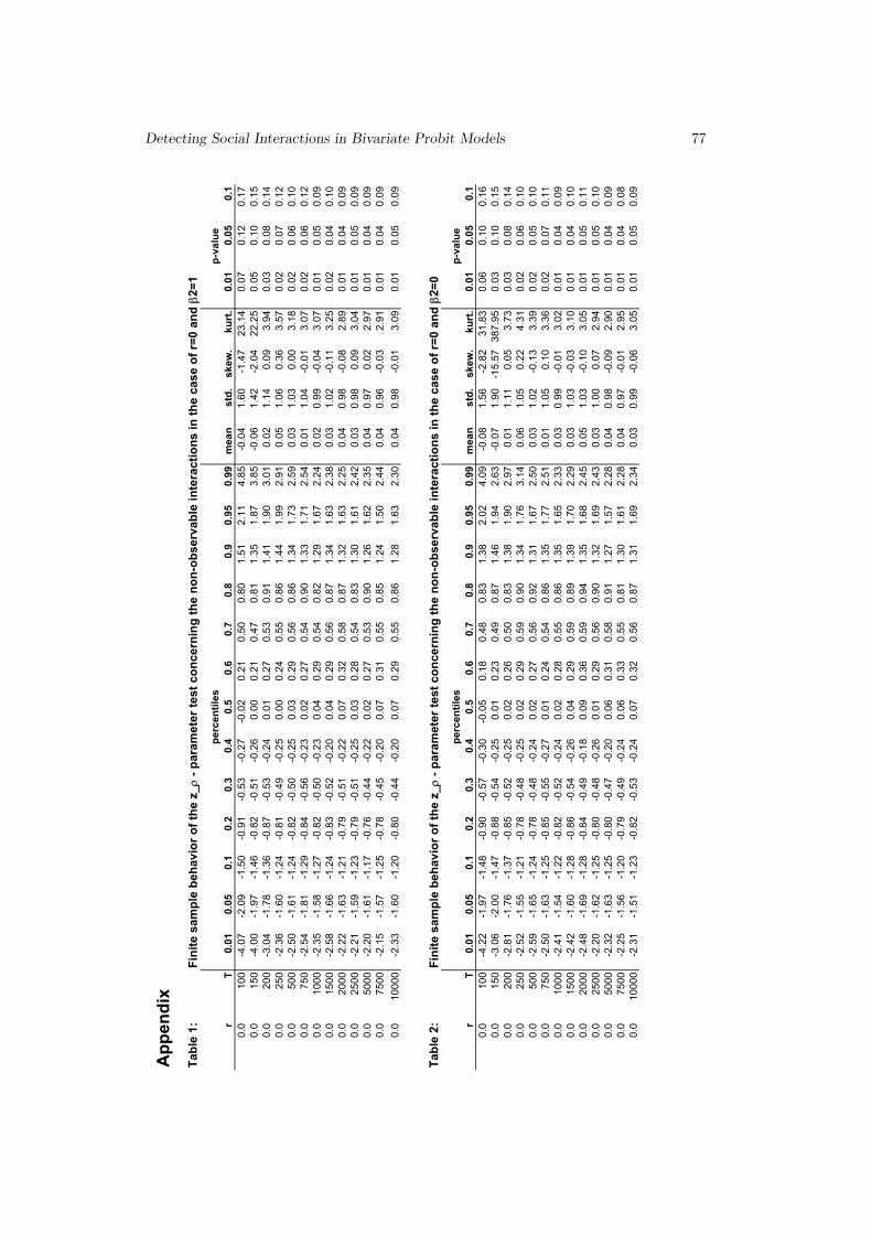
to one, β2 = 1. In Table 1 (see Appendix), we present percentiles of the simulated
zρ-statistic, some descriptive statistics like mean, standard deviation, skewness,
kurtosis, and the size of the test statistic with the nominal significance level equal
to 1, 5 and 10 percent.
Detecting Social Interactions in Bivariate Probit Models 73
-4
-2
0
2
4
-4 -2 0 2 4
Quantiles of t_rho
Quantile
s o
f N
orm
al
1000 obs
-4
-2
0
2
4
-6 -4 -2 0 2 4 6
Quantiles of t_rho
Quantile
s o
f N
orm
al
200 obs
-4
-2
0
2
4
-4 -2 0 2 4
Quantiles of t_rho
Quantile
s o
f N
orm
al
500 obs
Figure 3: QQ-Plots for t_rhorho=0, and T=200,500,1000
Figure 3: QQ-Plots for tρ, with ρ = 0 and T = 200, 500, 1000.
74 Johannes Jaenicke
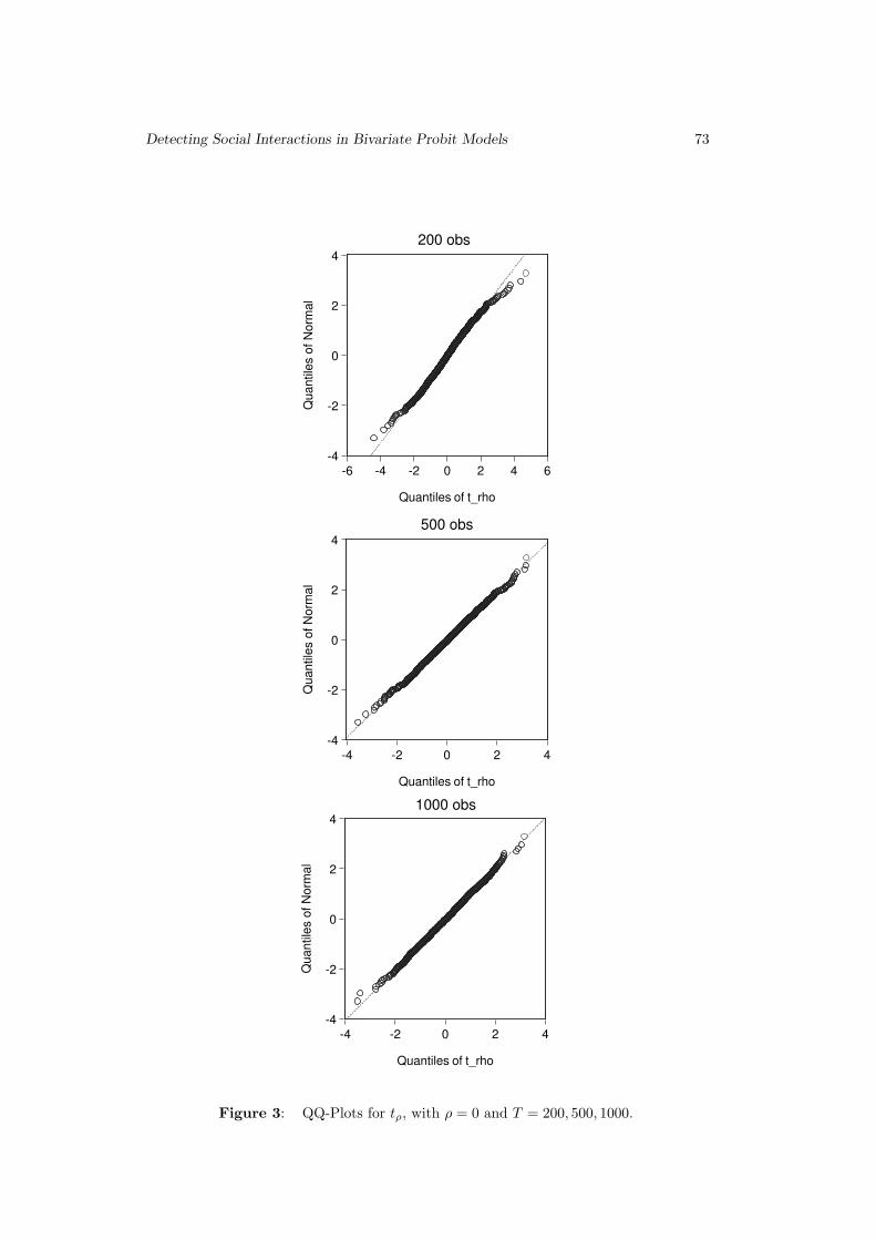
From Table 1, we see severe size distortions for the zρ-parameter test in
small data sets. In the case of T = 100, 150 observations, the test statistic is
excessively liberal. E.g., in the case of a nominal 5-percent level, the empirical size
is more than twice as high. The deviations from the nominal level become stronger
with a higher significance level. E.g., on the 1 percent level, the empirical size is
7 percent in the extreme case of T = 100 and 5 percent in the case of T = 150
observations. In these two cases the zρ-parameter test shows strong deviations
from normality. The distribution is negatively skewed and reveals strong excess
kurtosis. As expected, deviations from normality are not pronounced in the case
of medium size or huge data sets.
In Table 2, we present a set of experiments using our bivariate probit model
with an endogenous dummy variable but restricting the data generating mecha-
nism to β2 = 0, i.e., there is no endogenous dummy variable in the true model.
The results are generally in line with the ones of Table 1, but with stronger
deviations from normality in the small sample cases.
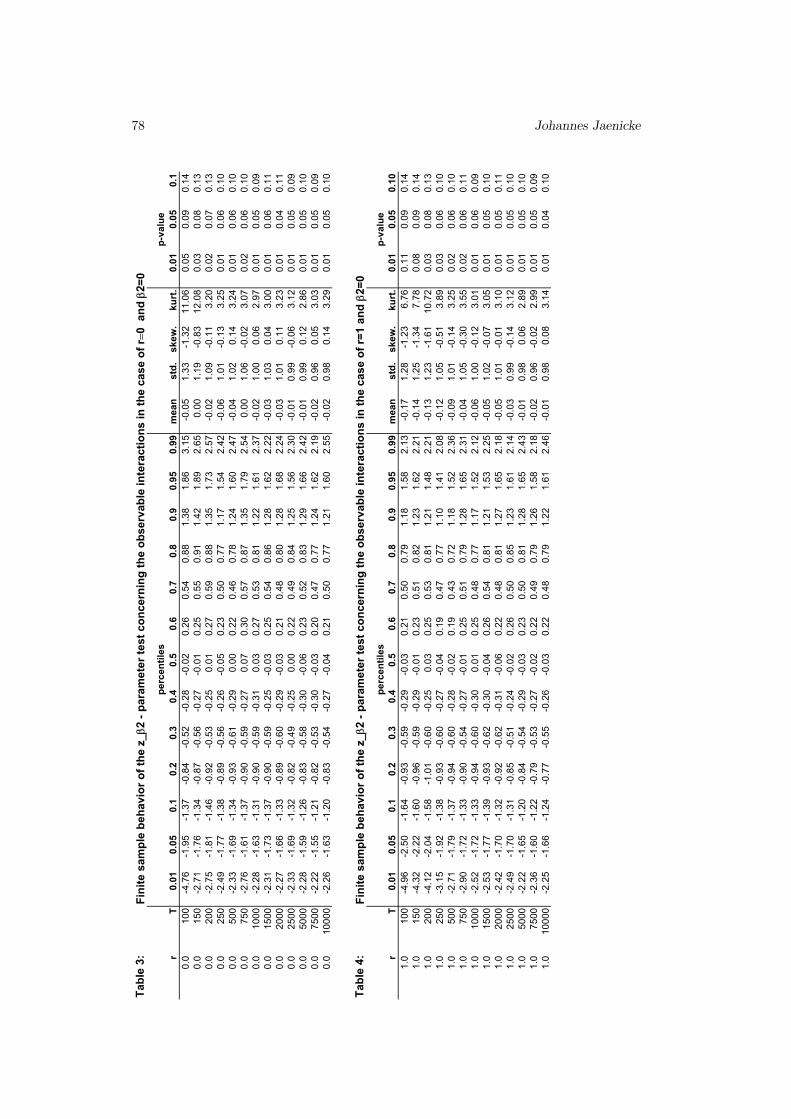
Using different correlation structures in Table 3 (r = 0) and Table 4 (r = 1),
we analyse the small sample behaviour of the test concerning the observable
interactions, the zβ2-parameter test. We find again some size distortions for data
sets with T ≤ 200 observations but no systematic influence of the correlation r.
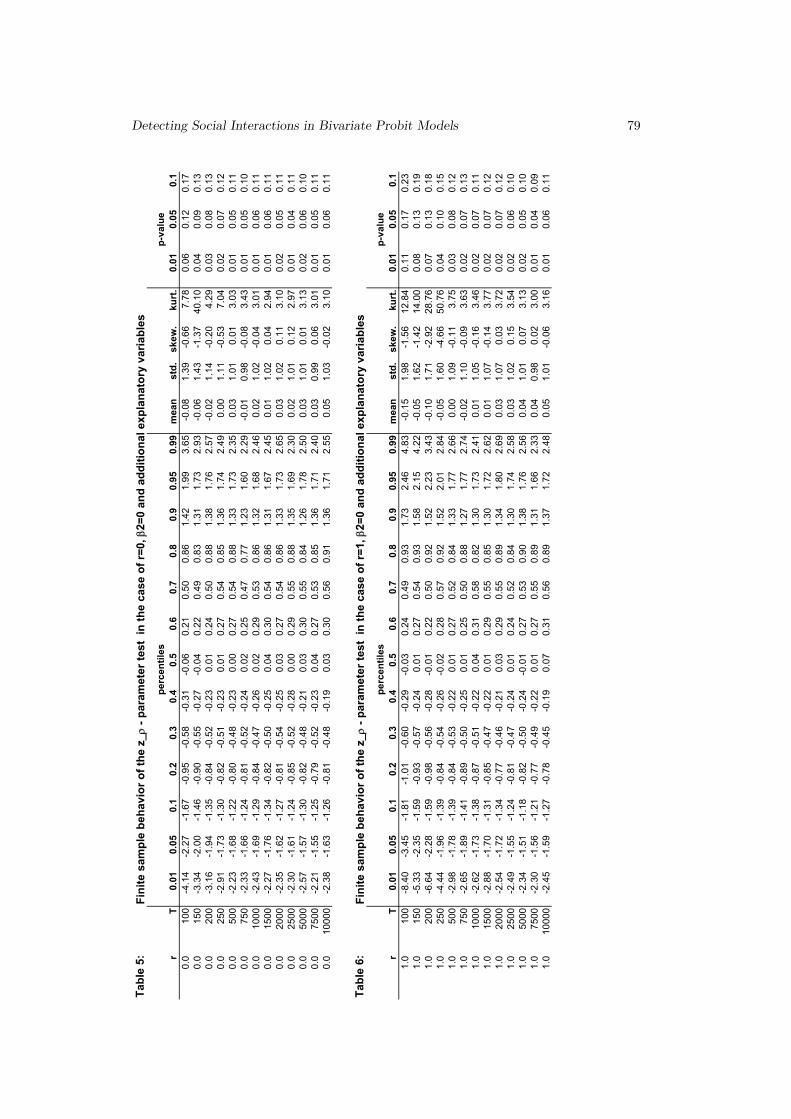
How will the size of the test statistic be affected if it is possible to include
the omitted variable vector [vI , vP ] as additional regressors? Does the correla-
tion r have an influence on the outcome of the test? Comparing Tables 2 and 5,
we see that the inclusion of additional explanatory variables makes the size dis-
tortions decrease only slightly. The comparison of Tables 5 and 6 makes clear
that correlation between explanatory variables negatively affects the size of the
zρ-test. In the case of r = 1, the empirical p-value of 10 percent is shifted to
23 percent in the T = 100 observation case. In this strong correlation case,
we need more than T = 2,000 observations to obtain good size properties of the
zρ-test. Summarizing Table 1 to 6, we find that in all small sample cases the test
statistic is too liberal.
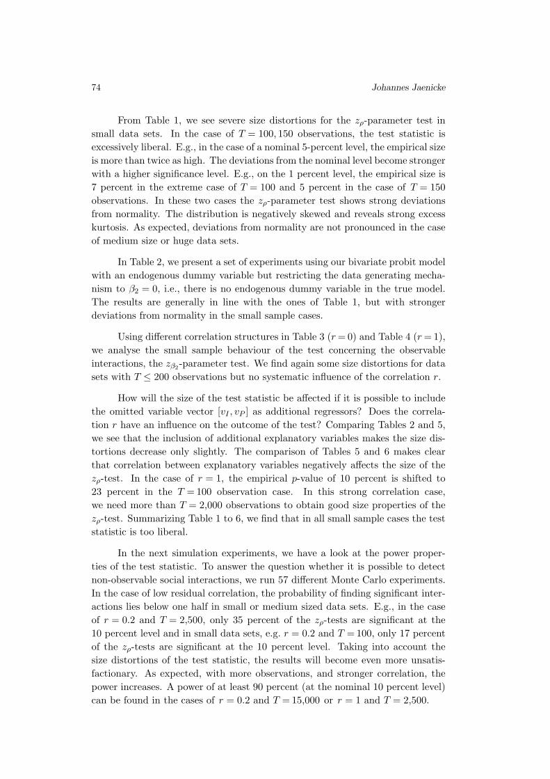
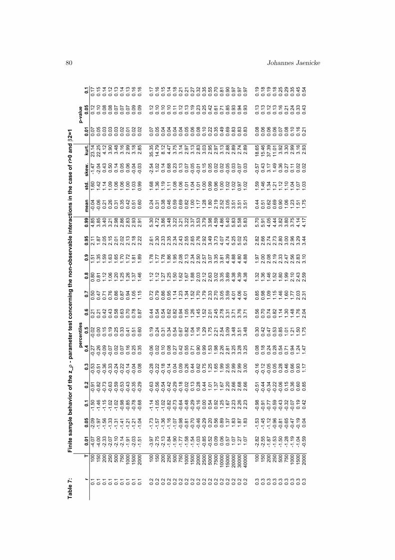
In the next simulation experiments, we have a look at the power proper-
ties of the test statistic. To answer the question whether it is possible to detect
non-observable social interactions, we run 57 different Monte Carlo experiments.
In the case of low residual correlation, the probability of finding significant inter-
actions lies below one half in small or medium sized data sets. E.g., in the case
of r = 0.2 and T = 2,500, only 35 percent of the zρ-tests are significant at the
10 percent level and in small data sets, e.g. r = 0.2 and T = 100, only 17 percent
of the zρ-tests are significant at the 10 percent level. Taking into account the
size distortions of the test statistic, the results will become even more unsatis-
factionary. As expected, with more observations, and stronger correlation, the
power increases. A power of at least 90 percent (at the nominal 10 percent level)
can be found in the cases of r = 0.2 and T = 15,000 or r = 1 and T = 2,500.
Detecting Social Interactions in Bivariate Probit Models 75
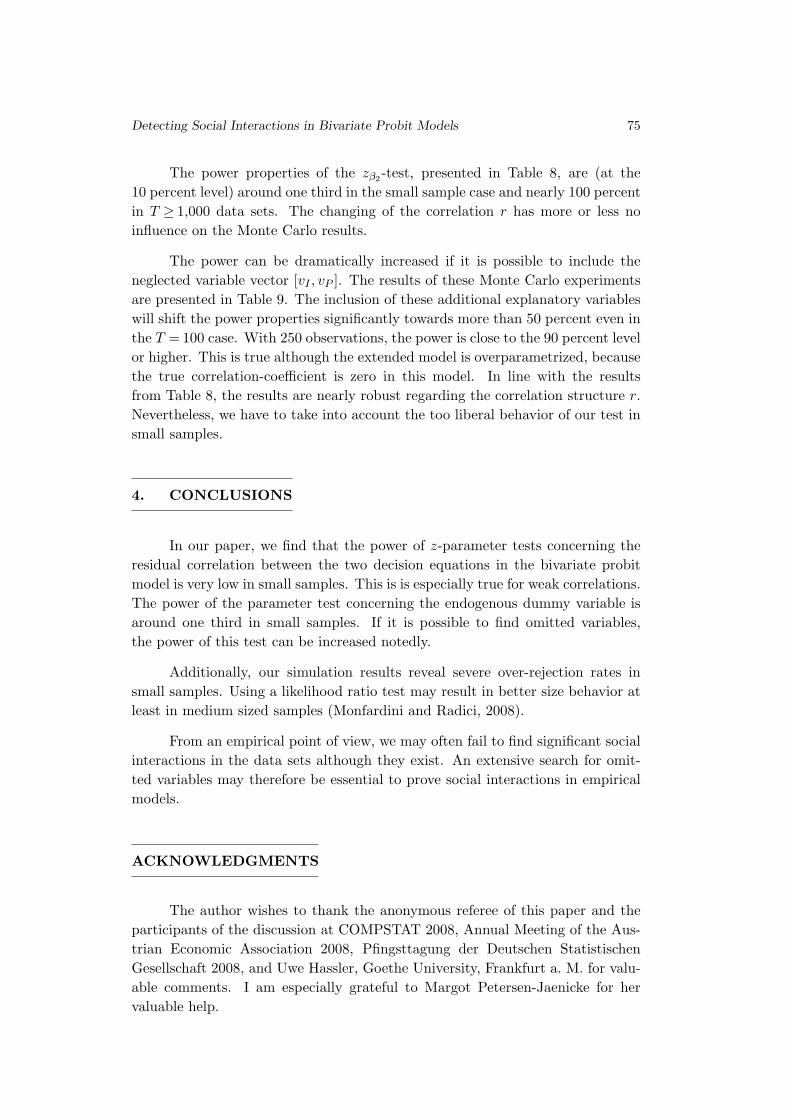
The power properties of the zβ2-test, presented in Table 8, are (at the
10 percent level) around one third in the small sample case and nearly 100 percent
in T ≥ 1,000 data sets. The changing of the correlation r has more or less no
influence on the Monte Carlo results.
The power can be dramatically increased if it is possible to include the
neglected variable vector [vI , vP ]. The results of these Monte Carlo experiments
are presented in Table 9. The inclusion of these additional explanatory variables
will shift the power properties significantly towards more than 50 percent even in
the T = 100 case. With 250 observations, the power is close to the 90 percent level
or higher. This is true although the extended model is overparametrized, because
the true correlation-coefficient is zero in this model. In line with the results
from Table 8, the results are nearly robust regarding the correlation structure r.
Nevertheless, we have to take into account the too liberal behavior of our test in
small samples.
4. CONCLUSIONS
In our paper, we find that the power of z-parameter tests concerning the
residual correlation between the two decision equations in the bivariate probit
model is very low in small samples. This is is especially true for weak correlations.
The power of the parameter test concerning the endogenous dummy variable is
around one third in small samples. If it is possible to find omitted variables,
the power of this test can be increased notedly.
Additionally, our simulation results reveal severe over-rejection rates in
small samples. Using a likelihood ratio test may result in better size behavior at
least in medium sized samples (Monfardini and Radici, 2008).
From an empirical point of view, we may often fail to find significant social
interactions in the data sets although they exist. An extensive search for omit-
ted variables may therefore be essential to prove social interactions in empirical
models.
ACKNOWLEDGMENTS
The author wishes to thank the anonymous referee of this paper and the
participants of the discussion at COMPSTAT 2008, Annual Meeting of the Aus-
trian Economic Association 2008, Pfingsttagung der Deutschen Statistischen
Gesellschaft 2008, and Uwe Hassler, Goethe University, Frankfurt a. M. for valu-
able comments. I am especially grateful to Margot Petersen-Jaenicke for her
valuable help.

76 Johannes Jaenicke
REFERENCES
[1] Brock, W.A. and Durlauf, S.N. (2001). Discrete choice with social interac-tions, Review of Economic Studies, 68, 235–260.
[2] Brock, W.A. and Durlauf, S.N. (2007). Identification of binary choice modelswith social interactions, Journal of Econometrics, 140, 52–75.
[3] Dean, J.M. (1995). Market disruption and the incidence of VERs under theMFA, Review of Economics and Statistics, 77, 383–388.
[4] Greene, W. (1998). Gender economics courses in liberal art colleges: Furtherresults, Journal of Economic Education, 29, 291–300.
[5] Greene, W.H. (2008). Econometric Analysis, 6th ed., Pearson, Prentice Hall.
[6] Heckman, J. (1978). Dummy endogenous variables in a simultaneous equationsystem, Econometrica, 9, 255–268.
[7] Jaenicke, J. (2004). Observable and Non-Observable Social Interactions in Labor
Supply, Discussion paper No. 2003/05, Rev. version, May 2004, University ofOsnabruck.
[8] Lollivier, S. (2001). Endogeneite d’une variable explicative dichotomique dans
le cadre d’un modele probit bivarie, Annales d’Economie et de Statistique, 62,251–269.
[9] Maddala, G.S. (1983). Limited Dependent and Quantitative Variables in
Econometrics, Cambridge University Press, Cambridge.
[10] Maddala, G.S. and Lee, L.-F. (1976). Recursive models with qualitative en-dogenous variables, Annals of Economic and Social Measurement, 5, 525–545.
[11] Manski, C.F. (1993). Identification of endogenous social effects: the reflectionproblem, Review of Economic Studies, 60, 531–542.
[12] McCullough,B.D. (1999). Econometric software reliability: EViews, LIMDEP,SHAZAM and TSP, Journal of Applied Econometrics, 14, 191–202.
[13] Monfardini, C. and Radice, R. (2008). Testing exogeneity in the bivariateprobit model: A Monte Carlo study, Oxford Bulletin of Economics and Statistics,70, 271–282.
[14] Murphy, A. (1995). Female labour force participation and unemployment inNorthern Ireland: Religion and family effects, Economic and Social Review, 27,67–84.
[15] Wilde, J. (2000). Identification of multiple equation probit models with endoge-nous dummy regressors, Economics Letters, 69, 309–312.
[16] Wilde, J. (2004). Estimating multiple equation hybrid models with endogenousdummy regressors, Statistica Neerlandica, 58, 296–312.
Detecting Social Interactions in Bivariate Probit Models 77
Ap
pen
dix
Tab
le 1
: rT
0.0
10.0
50.1
0.2
0.3
0.4
0.5
0.6
0.7
0.8
0.9
0.9
50.9
9m
ean
std
.skew
.ku
rt.
0.0
10.0
50.1
0.0
100
-4.07
-2.09
-1.50
-0.91
-0.53
-0.27
-0.02
0.21
0.50
0.80
1.51
2.11
4.85
-0.04
1.60
-1.47
23.14
0.07
0.12
0.17
0.0
150
-4.00
-1.97
-1.46
-0.82
-0.51
-0.26
0.00
0.21
0.47
0.81
1.35
1.87
3.85
-0.06
1.42
-2.04
22.25
0.05
0.10
0.15
0.0
200
-3.04
-1.78
-1.36
-0.87
-0.53
-0.24
0.01
0.27
0.53
0.91
1.41
1.90
3.01
0.02
1.14
0.09
3.94
0.03
0.08
0.14
0.0
250
-2.36
-1.60
-1.24
-0.81
-0.49
-0.25
0.00
0.24
0.55
0.86
1.44
1.99
2.91
0.05
1.06
0.36
3.57
0.02
0.07
0.12
0.0
500
-2.50
-1.61
-1.24
-0.82
-0.50
-0.25
0.03
0.29
0.56
0.86
1.34
1.73
2.59
0.03
1.03
0.00
3.18
0.02
0.06
0.10
0.0
750
-2.54
-1.81
-1.29
-0.84
-0.56
-0.23
0.02
0.27
0.54
0.90
1.33
1.71
2.54
0.01
1.04
-0.01
3.07
0.02
0.06
0.12
0.0
1000
-2.35
-1.58
-1.27
-0.82
-0.50
-0.23
0.04
0.29
0.54
0.82
1.29
1.67
2.24
0.02
0.99
-0.04
3.07
0.01
0.05
0.09
0.0
1500
-2.58
-1.66
-1.24
-0.83
-0.52
-0.20
0.04
0.29
0.56
0.87
1.34
1.63
2.38
0.03
1.02
-0.11
3.25
0.02
0.04
0.10
0.0
2000
-2.22
-1.63
-1.21
-0.79
-0.51
-0.22
0.07
0.32
0.58
0.87
1.32
1.63
2.25
0.04
0.98
-0.08
2.89
0.01
0.04
0.09
0.0
2500
-2.21
-1.59
-1.23
-0.79
-0.51
-0.25
0.03
0.28
0.54
0.83
1.30
1.61
2.42
0.03
0.98
0.09
3.04
0.01
0.05
0.09
0.0
5000
-2.20
-1.61
-1.17
-0.76
-0.44
-0.22
0.02
0.27
0.53
0.90
1.26
1.62
2.35
0.04
0.97
0.02
2.97
0.01
0.04
0.09
0.0
7500
-2.15
-1.57
-1.25
-0.78
-0.45
-0.20
0.07
0.31
0.55
0.85
1.24
1.50
2.44
0.04
0.96
-0.03
2.91
0.01
0.04
0.09
0.0
10000
-2.33
-1.60
-1.20
-0.80
-0.44
-0.20
0.07
0.29
0.55
0.86
1.28
1.63
2.30
0.04
0.98
-0.01
3.09
0.01
0.05
0.09
Tab
le 2
: rT
0.0
10.0
50.1
0.2
0.3
0.4
0.5
0.6
0.7
0.8
0.9
0.9
50.9
9m
ean
std
.skew
.ku
rt.
0.0
10.0
50.1
0.0
100
-4.22
-1.97
-1.48
-0.90
-0.57
-0.30
-0.05
0.18
0.48
0.83
1.38
2.02
4.09
-0.08
1.56
-2.82
31.83
0.06
0.10
0.16
0.0
150
-3.06
-2.00
-1.47
-0.88
-0.54
-0.25
0.01
0.23
0.49
0.87
1.46
1.94
2.63
-0.07
1.90-15.57387.95
0.03
0.10
0.15
0.0
200
-2.81
-1.76
-1.37
-0.85
-0.52
-0.25
0.02
0.26
0.50
0.83
1.38
1.90
2.97
0.01
1.11
0.05
3.73
0.03
0.08
0.14
0.0
250
-2.52
-1.55
-1.21
-0.78
-0.48
-0.25
0.02
0.29
0.59
0.90
1.34
1.76
3.14
0.06
1.05
0.22
4.31
0.02
0.06
0.10
0.0
500
-2.59
-1.65
-1.24
-0.78
-0.48
-0.24
0.02
0.27
0.56
0.92
1.31
1.67
2.50
0.03
1.02
-0.13
3.39
0.02
0.05
0.10
0.0
750
-2.50
-1.63
-1.25
-0.85
-0.55
-0.27
0.01
0.24
0.54
0.86
1.35
1.77
2.51
0.01
1.05
0.10
3.36
0.02
0.07
0.11
0.0
1000
-2.41
-1.54
-1.22
-0.82
-0.52
-0.24
0.02
0.28
0.55
0.86
1.35
1.65
2.33
0.03
0.99
-0.01
3.02
0.01
0.04
0.09
0.0
1500
-2.42
-1.60
-1.28
-0.86
-0.54
-0.26
0.04
0.29
0.59
0.89
1.39
1.70
2.29
0.03
1.03
-0.03
3.10
0.01
0.04
0.10
0.0
2000
-2.48
-1.69
-1.28
-0.84
-0.49
-0.18
0.09
0.36
0.59
0.94
1.35
1.68
2.45
0.05
1.03
-0.10
3.05
0.01
0.05
0.11
0.0
2500
-2.20
-1.62
-1.25
-0.80
-0.48
-0.26
0.01
0.29
0.56
0.90
1.32
1.69
2.43
0.03
1.00
0.07
2.94
0.01
0.05
0.10
0.0
5000
-2.32
-1.63
-1.25
-0.80
-0.47
-0.20
0.06
0.31
0.58
0.91
1.27
1.57
2.28
0.04
0.98
-0.09
2.90
0.01
0.04
0.09
0.0
7500
-2.25
-1.56
-1.20
-0.79
-0.49
-0.24
0.06
0.33
0.55
0.81
1.30
1.61
2.28
0.04
0.97
-0.01
2.95
0.01
0.04
0.08
0.0
10000
-2.31
-1.51
-1.23
-0.82
-0.53
-0.24
0.07
0.32
0.56
0.87
1.31
1.69
2.34
0.03
0.99
-0.06
3.05
0.01
0.05
0.09
p-v
alu
e
Fin
ite s
am
ple
beh
avio
r o
f th
e z
_ -
para
mete
r te
st
co
ncern
ing
th
e n
on
-ob
serv
ab
le i
nte
racti
on
s i
n t
he c
ase o
f r=
0 a
nd
!2=
0
perc
en
tile
sp
-valu
e
Fin
ite s
am
ple
beh
avio
r o
f th
e z
_ -
para
mete
r te
st
co
ncern
ing
th
e n
on
-ob
serv
ab
le i
nte
racti
on
s i
n t
he c
ase o
f r=
0 a
nd
!2=
1
perc
en
tile
s
78 Johannes JaenickeT
ab
le 3
: rT
0.0
10.0
50.1
0.2
0.3
0.4
0.5
0.6
0.7
0.8
0.9
0.9
50.9
9m
ean
std
.skew
.ku
rt.
0.0
10.0
50.1
0.0
100
-4.76
-1.95
-1.37
-0.84
-0.52
-0.28
-0.02
0.26
0.54
0.88
1.38
1.86
3.15
-0.05
1.33
-1.32
11.06
0.05
0.09
0.14
0.0
150
-2.71
-1.76
-1.34
-0.87
-0.56
-0.27
-0.01
0.25
0.55
0.91
1.42
1.89
2.65
0.00
1.19
-0.83
12.08
0.03
0.08
0.13
0.0
200
-2.75
-1.81
-1.46
-0.92
-0.53
-0.25
0.01
0.27
0.59
0.88
1.35
1.73
2.57
-0.02
1.09
-0.11
3.20
0.02
0.07
0.13
0.0
250
-2.49
-1.77
-1.38
-0.89
-0.56
-0.26
-0.05
0.23
0.50
0.77
1.17
1.54
2.42
-0.06
1.01
-0.13
3.25
0.01
0.06
0.10
0.0
500
-2.33
-1.69
-1.34
-0.93
-0.61
-0.29
0.00
0.22
0.46
0.78
1.24
1.60
2.47
-0.04
1.02
0.14
3.24
0.01
0.06
0.10
0.0
750
-2.76
-1.61
-1.37
-0.90
-0.59
-0.27
0.07
0.30
0.57
0.87
1.35
1.79
2.54
0.00
1.06
-0.02
3.07
0.02
0.06
0.10
0.0
1000
-2.28
-1.63
-1.31
-0.90
-0.59
-0.31
0.03
0.27
0.53
0.81
1.22
1.61
2.37
-0.02
1.00
0.06
2.97
0.01
0.05
0.09
0.0
1500
-2.31
-1.73
-1.37
-0.90
-0.59
-0.25
-0.03
0.25
0.54
0.86
1.28
1.62
2.22
-0.03
1.03
0.04
3.00
0.01
0.06
0.11
0.0
2000
-2.27
-1.66
-1.33
-0.89
-0.60
-0.29
-0.03
0.21
0.48
0.80
1.28
1.68
2.24
-0.03
1.01
0.11
3.23
0.01
0.04
0.11
0.0
2500
-2.33
-1.69
-1.32
-0.82
-0.49
-0.25
0.00
0.22
0.49
0.84
1.25
1.56
2.30
-0.01
0.99
-0.06
3.12
0.01
0.05
0.09
0.0
5000
-2.28
-1.59
-1.26
-0.83
-0.58
-0.30
-0.06
0.23
0.52
0.83
1.29
1.66
2.42
-0.01
0.99
0.12
2.86
0.01
0.05
0.10
0.0
7500
-2.22
-1.55
-1.21
-0.82
-0.53
-0.30
-0.03
0.20
0.47
0.77
1.24
1.62
2.19
-0.02
0.96
0.05
3.03
0.01
0.05
0.09
0.0
10000
-2.26
-1.63
-1.20
-0.83
-0.54
-0.27
-0.04
0.21
0.50
0.77
1.21
1.60
2.55
-0.02
0.98
0.14
3.29
0.01
0.05
0.10
rT
0.0
10.0
50.1
0.2
0.3
0.4
0.5
0.6
0.7
0.8
0.9
0.9
50.9
9m
ean
std
.skew
.ku
rt.
0.0
10.0
50.1
0
1.0
100
-4.96
-2.50
-1.64
-0.93
-0.59
-0.29
-0.03
0.21
0.50
0.79
1.18
1.58
2.13
-0.17
1.28
-1.23
6.76
0.11
0.09
0.14
1.0
150
-4.32
-2.22
-1.60
-0.96
-0.59
-0.29
-0.01
0.23
0.51
0.82
1.23
1.62
2.21
-0.14
1.25
-1.34
7.78
0.08
0.09
0.14
1.0
200
-4.12
-2.04
-1.58
-1.01
-0.60
-0.25
0.03
0.25
0.53
0.81
1.21
1.48
2.21
-0.13
1.23
-1.61
10.72
0.03
0.08
0.13
1.0
250
-3.15
-1.92
-1.38
-0.93
-0.60
-0.27
-0.04
0.19
0.47
0.77
1.10
1.41
2.08
-0.12
1.05
-0.51
3.89
0.03
0.06
0.10
1.0
500
-2.71
-1.79
-1.37
-0.94
-0.60
-0.28
-0.02
0.19
0.43
0.72
1.18
1.52
2.36
-0.09
1.01
-0.14
3.25
0.02
0.06
0.10
1.0
750
-2.90
-1.72
-1.33
-0.90
-0.54
-0.27
-0.01
0.25
0.51
0.79
1.28
1.65
2.31
-0.04
1.05
-0.30
3.55
0.02
0.06
0.11
1.0
1000
-2.52
-1.72
-1.33
-0.94
-0.60
-0.30
0.01
0.25
0.48
0.77
1.17
1.52
2.12
-0.06
1.00
-0.12
3.01
0.01
0.06
0.09
1.0
1500
-2.53
-1.77
-1.39
-0.93
-0.62
-0.30
-0.04
0.26
0.54
0.81
1.21
1.53
2.25
-0.05
1.02
-0.07
3.05
0.01
0.05
0.10
1.0
2000
-2.42
-1.70
-1.32
-0.92
-0.62
-0.31
-0.06
0.22
0.48
0.81
1.27
1.65
2.18
-0.05
1.01
-0.01
3.10
0.01
0.05
0.11
1.0
2500
-2.49
-1.70
-1.31
-0.85
-0.51
-0.24
-0.02
0.26
0.50
0.85
1.23
1.61
2.14
-0.03
0.99
-0.14
3.12
0.01
0.05
0.10
1.0
5000
-2.22
-1.65
-1.20
-0.84
-0.54
-0.29
-0.03
0.23
0.50
0.81
1.28
1.65
2.43
-0.01
0.98
0.06
2.89
0.01
0.05
0.10
1.0
7500
-2.36
-1.60
-1.22
-0.79
-0.53
-0.27
-0.02
0.22
0.49
0.79
1.26
1.58
2.18
-0.02
0.96
-0.02
2.99
0.01
0.05
0.09
1.0
10000
-2.25
-1.66
-1.24
-0.77
-0.55
-0.26
-0.03
0.22
0.48
0.79
1.22
1.61
2.46
-0.01
0.98
0.08
3.14
0.01
0.04
0.10
Tab
le 4
:F
init
e s
am
ple
beh
avio
r o
f th
e z
_ 2 -
para
mete
r te
st
co
ncern
ing
th
e o
bserv
ab
le i
nte
racti
on
s i
n t
he c
ase o
f r=
1 a
nd
2=
0
Fin
ite s
am
ple
beh
avio
r o
f th
e z
_ 2 -
para
mete
r te
st
co
ncern
ing
th
e o
bserv
ab
le i
nte
racti
on
s i
n t
he c
ase o
f r!
0
an
d
2=
0
perc
en
tile
sp
-valu
e
perc
en
tile
sp
-valu
e
Detecting Social Interactions in Bivariate Probit Models 79
rT
0.0
10.0
50.1
0.2
0.3
0.4
0.5
0.6
0.7
0.8
0.9
0.9
50.9
9m
ean
std
.skew
.ku
rt.
0.0
10.0
50.1
0.0
100
-4.14
-2.27
-1.67
-0.95
-0.58
-0.31
-0.06
0.21
0.50
0.86
1.42
1.99
3.65
-0.08
1.39
-0.66
7.78
0.06
0.12
0.17
0.0
150
-3.34
-2.00
-1.46
-0.90
-0.55
-0.27
-0.04
0.22
0.49
0.83
1.31
1.73
2.93
-0.06
1.43
-1.37
40.10
0.04
0.09
0.13
0.0
200
-3.16
-1.94
-1.35
-0.84
-0.52
-0.23
0.01
0.24
0.50
0.88
1.38
1.76
2.57
-0.02
1.14
-0.20
4.29
0.03
0.08
0.13
0.0
250
-2.91
-1.73
-1.30
-0.82
-0.51
-0.23
0.01
0.27
0.54
0.85
1.36
1.74
2.49
0.00
1.11
-0.53
7.04
0.02
0.07
0.12
0.0
500
-2.23
-1.68
-1.22
-0.80
-0.48
-0.23
0.00
0.27
0.54
0.88
1.33
1.73
2.35
0.03
1.01
0.01
3.03
0.01
0.05
0.11
0.0
750
-2.33
-1.66
-1.24
-0.81
-0.52
-0.24
0.02
0.25
0.47
0.77
1.23
1.60
2.29
-0.01
0.98
-0.08
3.43
0.01
0.05
0.10
0.0
1000
-2.43
-1.69
-1.29
-0.84
-0.47
-0.26
0.02
0.29
0.53
0.86
1.32
1.68
2.46
0.02
1.02
-0.04
3.01
0.01
0.06
0.11
0.0
1500
-2.27
-1.76
-1.34
-0.82
-0.50
-0.25
0.04
0.30
0.54
0.86
1.31
1.67
2.45
0.01
1.02
0.04
2.94
0.01
0.06
0.11
0.0
2000
-2.35
-1.62
-1.27
-0.81
-0.54
-0.25
0.03
0.27
0.54
0.86
1.33
1.73
2.65
0.03
1.02
0.11
3.10
0.02
0.05
0.11
0.0
2500
-2.30
-1.61
-1.24
-0.85
-0.52
-0.28
0.00
0.29
0.55
0.88
1.35
1.69
2.30
0.02
1.01
0.12
2.97
0.01
0.04
0.11
0.0
5000
-2.57
-1.57
-1.30
-0.82
-0.48
-0.21
0.03
0.30
0.55
0.84
1.26
1.78
2.50
0.03
1.01
0.01
3.13
0.02
0.06
0.10
0.0
7500
-2.21
-1.55
-1.25
-0.79
-0.52
-0.23
0.04
0.27
0.53
0.85
1.36
1.71
2.40
0.03
0.99
0.06
3.01
0.01
0.05
0.11
0.0
10000
-2.38
-1.63
-1.26
-0.81
-0.48
-0.19
0.03
0.30
0.56
0.91
1.36
1.71
2.55
0.05
1.03
-0.02
3.10
0.01
0.06
0.11
rT
0.0
10.0
50.1
0.2
0.3
0.4
0.5
0.6
0.7
0.8
0.9
0.9
50.9
9m
ean
std
.skew
.ku
rt.
0.0
10.0
50.1
1.0
100
-8.40
-3.45
-1.81
-1.01
-0.60
-0.29
-0.03
0.24
0.49
0.93
1.73
2.46
4.83
-0.15
1.98
-1.56
12.84
0.11
0.17
0.23
1.0
150
-5.33
-2.35
-1.59
-0.93
-0.57
-0.24
0.01
0.27
0.54
0.93
1.58
2.15
4.22
-0.05
1.62
-1.42
14.00
0.08
0.13
0.19
1.0
200
-6.64
-2.28
-1.59
-0.98
-0.56
-0.28
-0.01
0.22
0.50
0.92
1.52
2.23
3.43
-0.10
1.71
-2.92
28.76
0.07
0.13
0.18
1.0
250
-4.44
-1.96
-1.39
-0.84
-0.54
-0.26
-0.02
0.28
0.57
0.92
1.52
2.01
2.84
-0.05
1.60
-4.66
50.76
0.04
0.10
0.15
1.0
500
-2.98
-1.78
-1.39
-0.84
-0.53
-0.22
0.01
0.27
0.52
0.84
1.33
1.77
2.66
0.00
1.09
-0.11
3.75
0.03
0.08
0.12
1.0
750
-2.65
-1.89
-1.41
-0.89
-0.50
-0.25
0.01
0.25
0.50
0.88
1.27
1.77
2.74
-0.02
1.10
-0.09
3.63
0.02
0.07
0.13
1.0
1000
-2.62
-1.73
-1.38
-0.87
-0.51
-0.22
0.04
0.31
0.58
0.82
1.30
1.73
2.41
0.01
1.05
-0.16
3.46
0.02
0.07
0.11
1.0
1500
-2.88
-1.70
-1.31
-0.85
-0.47
-0.22
0.01
0.29
0.55
0.85
1.30
1.72
2.62
0.01
1.07
-0.14
3.77
0.02
0.07
0.12
1.0
2000
-2.54
-1.72
-1.34
-0.77
-0.46
-0.21
0.03
0.29
0.55
0.89
1.34
1.80
2.69
0.03
1.07
0.03
3.72
0.02
0.07
0.12
1.0
2500
-2.49
-1.55
-1.24
-0.81
-0.47
-0.24
0.01
0.24
0.52
0.84
1.30
1.74
2.58
0.03
1.02
0.15
3.54
0.02
0.06
0.10
1.0
5000
-2.34
-1.51
-1.18
-0.82
-0.50
-0.24
-0.01
0.27
0.53
0.90
1.38
1.76
2.56
0.04
1.01
0.07
3.13
0.02
0.05
0.10
1.0
7500
-2.30
-1.56
-1.21
-0.77
-0.49
-0.22
0.01
0.27
0.55
0.89
1.31
1.66
2.33
0.04
0.98
0.02
3.00
0.01
0.04
0.09
1.0
10000
-2.45
-1.59
-1.27
-0.78
-0.45
-0.19
0.07
0.31
0.56
0.89
1.37
1.72
2.48
0.05
1.01
-0.06
3.16
0.01
0.06
0.11
Tab
le 6
:F
init
e s
am
ple
beh
avio
r o
f th
e z
_ -
para
mete
r te
st
in
th
e c
ase o
f r=
1, !2=
0 a
nd
ad
dit
ion
al
exp
lan
ato
ry v
ari
ab
les
Tab
le 5
:F
init
e s
am
ple
beh
avio
r o
f th
e z
_ -
para
mete
r te
st
in
th
e c
ase o
f r=
0, !2=
0 a
nd
ad
dit
ion
al
exp
lan
ato
ry v
ari
ab
les
perc
en
tile
sp
-valu
e
perc
en
tile
sp
-valu
e
80 Johannes JaenickeT
ab
le 7
: rT
0.0
10.0
50.1
0.2
0.3
0.4
0.5
0.6
0.7
0.8
0.9
0.9
50.9
9m
ean
std
.skew
.ku
rt.
0.0
10.0
50.1
0.1
100
-4.07
-2.09
-1.50
-0.91
-0.53
-0.27
-0.02
0.21
0.50
0.80
1.51
2.11
4.85
-0.04
1.60
-1.47
23.14
0.07
0.12
0.17
0.1
150
-4.00
-1.97
-1.46
-0.82
-0.51
-0.26
0.00
0.21
0.47
0.81
1.35
1.87
3.85
-0.06
1.42
-2.04
22.25
0.05
0.10
0.15
0.1
200
-2.33
-1.56
-1.15
-0.73
-0.36
-0.09
0.15
0.42
0.71
1.12
1.59
2.05
3.40
0.21
1.14
0.43
4.12
0.03
0.08
0.14
0.1
250
-2.07
-1.33
-1.02
-0.63
-0.33
-0.07
0.19
0.43
0.76
1.06
1.63
2.15
3.21
0.26
1.09
0.50
3.90
0.03
0.08
0.12
0.1
500
-2.10
-1.31
-1.02
-0.59
-0.24
0.02
0.25
0.58
0.86
1.20
1.65
2.01
2.98
0.31
1.06
0.14
3.48
0.03
0.07
0.13
0.1
750
-2.14
-1.41
-0.98
-0.53
-0.22
0.07
0.33
0.63
0.87
1.25
1.70
2.02
2.86
0.35
1.06
0.05
3.16
0.02
0.07
0.14
0.1
1000
-1.91
-1.21
-0.85
-0.43
-0.14
0.16
0.41
0.70
0.94
1.26
1.72
2.13
2.83
0.42
1.00
0.06
2.99
0.01
0.07
0.13
0.1
1500
-2.03
-1.21
-0.78
-0.35
-0.04
0.25
0.51
0.78
1.05
1.37
1.81
2.18
2.93
0.51
1.03
-0.04
3.18
0.02
0.09
0.16
0.1
2000
-1.51
-1.04
-0.68
-0.29
0.08
0.35
0.60
0.87
1.15
1.46
1.89
2.22
2.91
0.60
0.99
-0.03
2.85
0.02
0.09
0.16
0.2
100
-3.97
-1.73
-1.14
-0.63
-0.28
-0.06
0.19
0.44
0.72
1.12
1.78
2.61
5.30
0.24
1.68
-2.54
35.35
0.07
0.12
0.17
0.2
150
-2.75
-1.57
-1.05
-0.56
-0.22
0.02
0.24
0.54
0.79
1.12
1.77
2.30
4.72
0.31
1.36
1.02
14.79
0.05
0.10
0.16
0.2
200
-2.13
-1.36
-1.02
-0.54
-0.18
0.10
0.31
0.54
0.86
1.27
1.78
2.33
3.86
0.38
1.19
0.14
8.12
0.04
0.10
0.15
0.2
250
-1.84
-1.16
-0.82
-0.42
-0.14
0.08
0.34
0.62
0.95
1.25
1.86
2.35
3.48
0.46
1.11
0.68
4.47
0.04
0.10
0.14
0.2
500
-1.90
-1.07
-0.73
-0.29
0.04
0.27
0.54
0.82
1.14
1.50
1.95
2.34
3.22
0.59
1.08
0.23
3.75
0.04
0.11
0.18
0.2
750
-1.77
-0.98
-0.64
-0.18
0.09
0.42
0.67
0.94
1.23
1.62
2.08
2.43
3.21
0.69
1.06
0.13
3.14
0.04
0.12
0.21
0.2
1000
-1.58
-0.81
-0.48
-0.02
0.26
0.55
0.82
1.05
1.34
1.67
2.13
2.55
3.22
0.82
1.01
0.07
2.97
0.05
0.13
0.21
0.2
1500
-1.54
-0.70
-0.29
0.13
0.44
0.71
1.04
1.26
1.52
1.88
2.34
2.65
3.37
1.00
1.04
-0.05
3.13
0.06
0.19
0.27
0.2
2000
-1.03
-0.46
-0.16
0.28
0.62
0.90
1.16
1.45
1.70
2.03
2.50
2.76
3.53
1.17
1.01
-0.01
2.83
0.08
0.23
0.32
0.2
2500
-0.85
-0.29
0.00
0.44
0.75
0.99
1.29
1.52
1.79
2.12
2.57
2.92
3.79
1.28
1.00
0.15
3.03
0.10
0.25
0.35
0.2
5000
-0.52
0.20
0.54
1.01
1.25
1.53
1.75
2.01
2.33
2.63
3.07
3.49
3.98
1.80
0.99
0.05
2.95
0.22
0.42
0.55
0.2
7500
0.09
0.56
0.92
1.37
1.65
1.98
2.21
2.45
2.70
3.02
3.35
3.73
4.59
2.19
0.96
0.02
2.97
0.35
0.61
0.70
0.2
10000
0.06
0.89
1.25
1.67
1.99
2.26
2.54
2.78
3.05
3.35
3.81
4.07
4.86
2.52
1.00
0.02
3.13
0.49
0.71
0.81
0.2
15000
0.57
1.37
1.67
2.20
2.55
2.81
3.09
3.31
3.59
3.89
4.39
4.74
5.40
3.05
1.02
-0.05
2.88
0.69
0.85
0.90
0.2
20000
1.07
1.83
2.23
2.66
2.99
3.25
3.48
3.71
4.01
4.38
4.88
5.25
5.83
3.51
1.02
0.03
2.89
0.83
0.93
0.97
0.2
30000
1.27
1.87
2.26
2.68
2.99
3.28
3.51
3.76
4.06
4.39
4.80
5.02
5.58
3.51
0.97
-0.07
2.74
0.83
0.94
0.97
0.2
40000
1.07
1.83
2.23
2.66
3.00
3.25
3.48
3.71
4.01
4.38
4.88
5.25
5.83
3.51
1.02
0.03
2.89
0.83
0.93
0.97
0.3
100
-2.82
-1.53
-0.98
-0.51
-0.16
0.08
0.30
0.56
0.85
1.32
1.97
2.82
5.70
0.44
1.59
-0.57
18.65
0.08
0.13
0.19
0.3
150
-2.55
-1.45
-0.91
-0.44
-0.12
0.18
0.42
0.70
0.98
1.36
2.00
2.66
5.91
0.51
1.46
0.43
15.46
0.06
0.13
0.18
0.3
200
-1.87
-1.12
-0.77
-0.34
-0.05
0.24
0.47
0.74
1.09
1.46
2.08
2.74
4.05
0.62
1.34
3.17
37.39
0.06
0.12
0.19
0.3
250
-1.53
-0.96
-0.59
-0.22
0.05
0.28
0.53
0.82
1.15
1.52
2.19
2.73
4.44
0.69
1.21
1.49
11.01
0.06
0.13
0.18
0.3
500
-1.50
-0.81
-0.43
-0.06
0.28
0.54
0.85
1.14
1.46
1.80
2.33
2.80
3.82
0.90
1.12
0.36
3.92
0.07
0.16
0.25
0.3
750
-1.28
-0.65
-0.32
0.15
0.46
0.71
1.01
1.30
1.60
1.99
2.47
3.00
3.80
1.06
1.10
0.27
3.30
0.08
0.21
0.29
0.3
1000
-1.19
-0.47
-0.07
0.36
0.66
0.94
1.21
1.48
1.77
2.10
2.56
2.96
3.75
1.23
1.04
0.11
2.99
0.10
0.24
0.35
0.3
1500
-1.04
-0.19
0.19
0.60
0.93
1.24
1.50
1.76
2.03
2.43
2.83
3.29
4.14
1.51
1.07
0.02
3.16
0.16
0.33
0.45
0.3
2000
-0.59
0.04
0.42
0.85
1.17
1.47
1.75
2.04
2.31
2.59
3.10
3.44
4.17
1.75
1.03
0.02
2.93
0.21
0.43
0.54
Fin
ite s
am
ple
beh
avio
r o
f th
e z
_ -
para
mete
r te
st
co
ncern
ing
th
e n
on
-ob
serv
ab
le i
nte
racti
on
s i
n t
he c
ase o
f r>
0 a
nd
!2=
1
perc
en
tile
sp
-valu
e
Detecting Social Interactions in Bivariate Probit Models 81T
ab
le 7
(co
nt.
):
rT
0.0
10.0
50.1
0.2
0.3
0.4
0.5
0.6
0.7
0.8
0.9
0.9
50.9
9m
ean
std
.skew
.ku
rt.
0.0
10.0
50.1
0.4
100
-2.81
-1.31
-0.81
-0.37
-0.07
0.18
0.45
0.70
1.01
1.51
2.26
3.26
6.50
0.61
1.65
-0.26
17.31
0.09
0.16
0.20
0.4
150
-2.01
-1.23
-0.75
-0.27
0.03
0.32
0.56
0.86
1.16
1.51
2.21
3.12
6.33
0.73
1.77
2.89
68.17
0.07
0.14
0.20
0.4
200
-1.80
-1.00
-0.62
-0.19
0.13
0.41
0.67
0.96
1.28
1.65
2.36
3.15
5.05
0.83
1.45
3.56
40.80
0.08
0.16
0.22
0.4
250
-1.40
-0.81
-0.44
-0.03
0.24
0.48
0.77
1.04
1.38
1.79
2.41
3.06
4.63
0.92
1.31
2.63
27.92
0.09
0.16
0.23
0.4
500
-1.13
-0.56
-0.22
0.21
0.57
0.85
1.15
1.47
1.77
2.14
2.69
3.23
4.32
1.20
1.15
0.37
3.70
0.11
0.25
0.35
0.4
750
-0.85
-0.34
0.00
0.51
0.79
1.07
1.41
1.68
1.98
2.39
2.91
3.40
4.20
1.44
1.14
0.29
3.22
0.16
0.31
0.41
0.4
1000
-0.67
-0.08
0.32
0.71
1.10
1.36
1.63
1.92
2.23
2.55
3.01
3.47
4.31
1.66
1.07
0.15
3.03
0.19
0.38
0.50
0.4
1500
-0.69
0.29
0.60
1.09
1.44
1.75
2.01
2.26
2.60
2.95
3.43
3.86
4.77
2.02
1.10
0.04
3.09
0.31
0.53
0.62
0.4
2000
-0.04
0.62
0.98
1.44
1.77
2.04
2.31
2.64
2.90
3.20
3.70
4.10
4.88
2.33
1.06
0.07
3.03
0.42
0.63
0.74
0.5
100
-2.48
-1.06
-0.69
-0.23
0.07
0.28
0.55
0.85
1.16
1.62
2.48
3.32
5.40
0.76
1.50
0.99
8.17
0.11
0.18
0.22
0.5
150
-1.74
-1.02
-0.63
-0.14
0.22
0.46
0.72
1.04
1.35
1.74
2.54
3.45
7.56
0.98
2.23
11.31229.04
0.10
0.17
0.23
0.5
200
-1.60
-0.73
-0.45
0.00
0.29
0.57
0.82
1.17
1.51
1.93
2.65
3.42
5.49
1.03
1.41
1.93
14.00
0.11
0.19
0.27
0.5
250
-1.19
-0.59
-0.22
0.16
0.41
0.69
0.94
1.23
1.59
1.99
2.70
3.36
5.35
1.13
1.29
1.35
8.11
0.11
0.21
0.29
0.5
500
-0.90
-0.25
0.08
0.49
0.87
1.14
1.43
1.78
2.10
2.46
3.04
3.58
4.80
1.53
1.20
0.64
4.71
0.17
0.34
0.44
0.5
750
-0.63
0.03
0.39
0.83
1.13
1.47
1.78
2.04
2.38
2.81
3.38
3.90
4.89
1.83
1.19
0.47
3.72
0.25
0.44
0.55
0.5
1000
-0.22
0.34
0.76
1.17
1.50
1.77
2.06
2.37
2.71
3.01
3.52
4.08
4.90
2.11
1.11
0.25
3.16
0.34
0.53
0.63
0.5
1500
-0.25
0.78
1.11
1.59
1.90
2.24
2.54
2.82
3.16
3.56
4.04
4.54
5.53
2.57
1.15
0.16
3.11
0.48
0.69
0.79
0.5
2000
0.46
1.17
1.55
2.05
2.34
2.61
2.98
3.26
3.54
3.90
4.38
4.83
5.77
2.97
1.11
0.16
3.11
0.62
0.82
0.89
0.5
2500
0.99
1.57
1.88
2.33
2.69
2.94
3.28
3.54
3.83
4.22
4.74
5.13
6.19
3.30
1.11
0.28
3.18
0.74
0.89
0.94
0.5
5000
2.20
2.88
3.27
3.71
4.08
4.34
4.59
4.91
5.21
5.59
6.11
6.53
7.31
4.65
1.10
0.12
2.91
0.98
1.00
1.00
0.5
7500
3.26
3.85
4.29
4.71
5.15
5.45
5.72
5.96
6.25
6.55
7.01
7.34
8.30
5.68
1.07
0.00
2.92
1.00
1.00
1.00
0.5
10000
4.01
4.74
5.12
5.58
5.97
6.29
6.54
6.83
7.11
7.45
7.92
8.34
9.33
6.54
1.11
0.12
3.20
1.00
1.00
1.00
Fin
ite s
am
ple
beh
avio
r o
f th
e z
_ -
para
mete
r te
st
co
ncern
ing
th
e n
on
-ob
serv
ab
le i
nte
racti
on
s i
n t
he c
ase o
f r>
0 a
nd
!2=
1
perc
en
tile
sp
-valu
e

82 Johannes JaenickeT
ab
le 8
:
rT
0.0
10.0
50.1
0.2
0.3
0.4
0.5
0.6
0.7
0.8
0.9
0.9
50.9
9m
ean
std
.skew
.ku
rt.
0.0
10.0
50.1
0.0
100
-2.08
-0.67
-0.15
0.28
0.57
0.84
1.13
1.41
1.70
2.16
3.06
3.66
5.69
1.27
1.47
0.30
8.07
0.15
0.25
0.33
0.0
150
-1.28
-0.21
0.16
0.60
0.89
1.17
1.40
1.67
2.04
2.48
3.15
3.93
5.80
1.59
1.39
1.59
10.10
0.19
0.32
0.41
0.0
200
-0.73
-0.04
0.31
0.76
1.05
1.30
1.61
1.90
2.21
2.63
3.36
3.99
5.21
1.73
1.24
0.78
4.84
0.21
0.37
0.48
0.0
250
-0.48
0.03
0.50
0.99
1.33
1.58
1.82
2.06
2.31
2.75
3.24
3.73
4.89
1.86
1.09
0.32
3.48
0.24
0.45
0.58
0.0
500
0.07
0.88
1.23
1.73
2.05
2.34
2.57
2.83
3.15
3.49
3.99
4.56
5.35
2.62
1.09
0.30
3.58
0.50
0.72
0.83
0.0
750
0.94
1.57
1.85
2.32
2.60
2.89
3.19
3.50
3.79
4.20
4.69
5.25
6.13
3.25
1.13
0.37
3.24
0.71
0.88
0.94
0.0
1000
1.40
2.07
2.44
2.85
3.15
3.39
3.65
3.94
4.27
4.63
5.13
5.63
6.39
3.73
1.06
0.23
2.93
0.86
0.96
0.98
0.0
1500
2.18
2.88
3.15
3.61
3.89
4.26
4.51
4.75
5.12
5.44
6.00
6.45
7.44
4.55
1.11
0.34
3.28
0.97
1.00
1.00
0.0
2000
2.95
3.55
3.94
4.38
4.70
4.93
5.18
5.48
5.77
6.11
6.60
7.05
7.80
5.24
1.04
0.18
3.12
0.99
1.00
1.00
0.0
2500
3.39
4.15
4.61
5.00
5.31
5.59
5.85
6.16
6.43
6.79
7.23
7.72
8.40
5.89
1.06
0.06
3.04
1.00
1.00
1.00
0.0
5000
6.02
6.64
6.97
7.37
7.71
8.02
8.30
8.58
8.83
9.19
9.67
10.07
10.73
8.30
1.05
0.09
2.75
1.00
1.00
1.00
0.0
7500
7.86
8.52
8.89
9.32
9.63
9.86
10.12
10.41
10.73
11.07
11.51
11.89
12.50
10.17
1.02
0.05
2.79
1.00
1.00
1.00
0.0
10000
9.20
10.09
10.43
10.85
11.16
11.45
11.72
11.99
12.26
12.61
13.06
13.48
14.49
11.74
1.05
0.08
3.16
1.00
1.00
1.00
0.1
100
-2.08
-0.67
-0.15
0.28
0.57
0.84
1.13
1.41
1.70
2.16
3.06
3.66
5.69
1.27
1.47
0.30
8.07
0.15
0.25
0.33
0.1
150
-1.28
-0.21
0.16
0.60
0.89
1.17
1.40
1.67
2.04
2.48
3.15
3.93
5.80
1.59
1.39
1.59
10.10
0.19
0.32
0.41
0.1
200
-0.78
-0.08
0.31
0.78
1.03
1.30
1.59
1.89
2.19
2.61
3.28
3.85
4.86
1.70
1.18
0.53
3.77
0.21
0.38
0.48
0.1
250
-0.42
0.07
0.46
0.98
1.29
1.58
1.80
2.03
2.30
2.71
3.19
3.68
4.89
1.84
1.08
0.30
3.57
0.24
0.43
0.57
0.1
500
0.12
0.95
1.23
1.71
2.05
2.30
2.54
2.76
3.14
3.50
3.97
4.46
5.21
2.60
1.08
0.31
3.67
0.48
0.72
0.82
0.1
750
0.88
1.52
1.84
2.29
2.57
2.86
3.16
3.46
3.75
4.16
4.62
5.16
6.20
3.22
1.12
0.39
3.41
0.69
0.87
0.94
0.1
1000
1.38
2.09
2.41
2.83
3.12
3.35
3.62
3.91
4.20
4.59
5.11
5.51
6.20
3.70
1.04
0.24
2.93
0.86
0.96
0.98
0.1
1500
2.19
2.86
3.11
3.55
3.92
4.23
4.45
4.72
5.05
5.37
5.95
6.30
7.30
4.51
1.08
0.31
3.23
0.97
1.00
1.00
0.1
2000
2.93
3.57
3.91
4.32
4.65
4.90
5.15
5.42
5.73
6.10
6.51
6.94
7.61
5.19
1.03
0.17
3.14
1.00
1.00
1.00
0.2
100
-1.93
-0.62
-0.14
0.28
0.59
0.85
1.09
1.37
1.63
2.07
2.78
3.45
5.08
1.21
1.28
0.32
4.98
0.13
0.24
0.32
0.2
150
-1.25
-0.21
0.16
0.59
0.89
1.18
1.39
1.65
1.95
2.47
3.01
3.70
5.52
1.53
1.30
0.87
9.44
0.18
0.30
0.41
0.2
200
-0.80
-0.06
0.31
0.79
1.06
1.30
1.60
1.87
2.14
2.59
3.23
3.77
4.96
1.70
1.23
1.83
19.71
0.20
0.37
0.49
0.2
250
-0.47
0.08
0.50
1.01
1.34
1.59
1.81
2.03
2.27
2.66
3.16
3.60
4.58
1.83
1.06
0.25
3.54
0.22
0.43
0.57
0.2
500
0.10
0.95
1.23
1.73
2.02
2.31
2.56
2.75
3.14
3.46
3.93
4.33
5.13
2.58
1.06
0.29
3.78
0.49
0.72
0.82
0.2
750
0.85
1.51
1.84
2.30
2.56
2.86
3.14
3.45
3.73
4.12
4.55
5.02
6.13
3.19
1.09
0.35
3.32
0.70
0.87
0.93
0.2
1000
1.42
2.08
2.42
2.79
3.10
3.35
3.60
3.86
4.16
4.53
5.01
5.45
6.16
3.67
1.02
0.25
2.91
0.86
0.97
0.98
0.2
1500
2.14
2.82
3.13
3.52
3.90
4.19
4.43
4.68
4.99
5.32
5.84
6.23
7.12
4.46
1.05
0.29
3.20
0.97
1.00
1.00
0.2
2000
2.86
3.51
3.89
4.26
4.65
4.87
5.09
5.34
5.66
6.00
6.49
6.82
7.42
5.15
1.00
0.15
3.07
1.00
1.00
1.00
0.2
2500
3.40
4.15
4.48
4.94
5.25
5.48
5.76
6.03
6.30
6.60
7.06
7.48
8.21
5.78
1.01
0.06
3.06
1.00
1.00
1.00
0.2
5000
5.96
6.54
6.84
7.30
7.61
7.88
8.14
8.42
8.68
9.02
9.48
9.79
10.58
8.16
1.00
0.07
2.77
1.00
1.00
1.00
0.2
7500
7.74
8.39
8.75
9.19
9.48
9.73
9.94
10.22
10.51
10.83
11.29
11.62
12.27
9.99
0.97
0.04
2.82
1.00
1.00
1.00
0.2
10000
9.17
9.99
10.30
10.69
11.00
11.27
11.54
11.77
12.05
12.35
12.80
13.22
14.10
11.53
1.00
0.09
3.20
1.00
1.00
1.00
0.2
15000
11.79
12.47
12.80
13.25
13.57
13.87
14.12
14.39
14.67
15.02
15.56
15.93
16.46
14.15
1.04
0.07
2.73
1.00
1.00
1.00
0.2
20000
14.05
14.71
14.98
15.45
15.79
16.06
16.34
16.63
16.87
17.18
17.71
18.05
18.80
16.34
1.02
0.07
2.78
1.00
1.00
1.00
0.2
30000
14.19
14.79
15.09
15.50
15.80
16.05
16.27
16.57
16.90
17.21
17.64
18.00
18.68
16.35
0.99
0.16
3.02
1.00
1.00
1.00
0.2
40000
14.05
14.71
14.98
15.45
15.79
16.06
16.34
16.63
16.87
17.18
17.71
18.06
18.80
16.35
1.05
0.48
5.75
1.00
1.00
1.00
Fin
ite s
am
ple
beh
avio
r o
f th
e z
_ 2 -
para
mete
r te
st
co
ncern
ing
th
e n
on
-ob
serv
ab
le i
nte
racti
on
s i
n t
he c
ase o
f r
0 a
nd
2=
1
perc
en
tile
sp
-valu
e

Detecting Social Interactions in Bivariate Probit Models 83T
ab
le 8
(co
nt.
):
rT
0.0
10.0
50.1
0.2
0.3
0.4
0.5
0.6
0.7
0.8
0.9
0.9
50.9
9m
ean
std
.skew
.ku
rt.
0.0
10.0
50.1
0.3
100
-2.39
-0.64
-0.13
0.28
0.60
0.83
1.11
1.37
1.67
2.01
2.69
3.42
4.69
1.18
1.27
-0.06
6.11
0.12
0.22
0.32
0.3
150
-1.24
-0.20
0.11
0.59
0.87
1.14
1.38
1.64
1.92
2.44
2.94
3.69
4.95
1.49
1.26
0.64
10.01
0.17
0.29
0.40
0.3
200
-0.70
-0.05
0.30
0.78
1.06
1.28
1.56
1.86
2.14
2.54
3.13
3.71
4.66
1.66
1.14
0.31
4.16
0.19
0.36
0.48
0.3
250
-0.51
0.07
0.52
1.00
1.30
1.59
1.79
2.01
2.24
2.64
3.10
3.57
4.60
1.81
1.04
0.15
3.83
0.21
0.43
0.57
0.3
500
0.11
0.90
1.22
1.70
1.99
2.31
2.51
2.77
3.08
3.40
3.88
4.27
5.14
2.56
1.05
0.27
3.84
0.47
0.71
0.82
0.3
750
0.93
1.56
1.83
2.27
2.56
2.83
3.10
3.40
3.68
4.04
4.54
5.02
5.86
3.16
1.07
0.32
3.32
0.70
0.88
0.94
0.3
1000
1.39
2.12
2.42
2.78
3.09
3.31
3.56
3.81
4.13
4.47
4.98
5.34
6.13
3.64
1.00
0.25
2.92
0.87
0.96
0.98
0.3
1500
2.10
2.81
3.13
3.51
3.88
4.16
4.38
4.66
4.97
5.27
5.81
6.09
7.09
4.43
1.03
0.25
3.22
0.97
1.00
1.00
0.3
2000
2.91
3.49
3.88
4.26
4.61
4.86
5.05
5.32
5.61
5.96
6.40
6.74
7.36
5.11
0.98
0.14
3.03
1.00
1.00
1.00
0.4
100
-1.93
-0.59
-0.14
0.27
0.60
0.82
1.10
1.34
1.61
1.96
2.58
3.32
4.68
1.16
1.26
-0.04
6.31
0.11
0.21
0.30
0.4
150
-1.17
-0.19
0.15
0.57
0.86
1.13
1.37
1.62
1.90
2.33
2.92
3.49
4.56
1.45
1.17
-0.08
5.84
0.17
0.28
0.39
0.4
200
-0.79
-0.07
0.30
0.79
1.04
1.30
1.58
1.81
2.10
2.53
3.11
3.51
4.64
1.64
1.13
0.05
5.61
0.19
0.35
0.47
0.4
250
-0.41
0.08
0.48
1.00
1.29
1.56
1.78
1.99
2.23
2.57
3.08
3.55
4.65
1.79
1.03
0.08
4.27
0.20
0.42
0.57
0.4
500
0.09
0.94
1.21
1.70
1.99
2.27
2.51
2.74
3.04
3.36
3.88
4.28
5.10
2.54
1.03
0.28
3.78
0.47
0.71
0.81
0.4
750
0.97
1.56
1.84
2.25
2.55
2.83
3.09
3.40
3.65
4.01
4.50
4.95
5.65
3.14
1.05
0.29
3.21
0.69
0.87
0.93
0.4
1000
1.37
2.13
2.37
2.79
3.06
3.29
3.54
3.81
4.10
4.44
4.95
5.32
6.05
3.62
0.98
0.24
2.97
0.86
0.97
0.98
0.4
1500
2.15
2.79
3.16
3.51
3.86
4.13
4.40
4.64
4.93
5.20
5.74
6.10
6.91
4.41
1.02
0.23
3.21
0.97
0.99
1.00
0.4
2000
2.89
3.50
3.89
4.30
4.58
4.82
5.04
5.30
5.57
5.89
6.32
6.66
7.35
5.09
0.96
0.14
3.13
1.00
1.00
1.00
0.5
100
-3.00
-0.62
-0.08
0.26
0.60
0.82
1.08
1.33
1.58
1.90
2.51
3.07
4.10
1.10
1.21
-0.72
7.76
0.11
0.20
0.29
0.5
150
-1.19
-0.15
0.16
0.60
0.87
1.14
1.34
1.59
1.89
2.31
2.85
3.45
4.51
1.44
1.18
0.32
9.53
0.16
0.28
0.38
0.5
200
-0.90
-0.07
0.33
0.77
1.05
1.30
1.59
1.82
2.09
2.47
3.03
3.48
4.53
1.61
1.10
-0.10
5.92
0.19
0.35
0.48
0.5
250
-0.45
0.12
0.53
1.01
1.31
1.56
1.79
1.99
2.21
2.56
3.00
3.41
4.19
1.78
1.00
-0.05
4.47
0.20
0.42
0.55
0.5
500
0.13
0.98
1.26
1.70
2.03
2.27
2.52
2.69
2.97
3.31
3.82
4.14
4.98
2.52
1.00
0.19
3.75
0.46
0.73
0.81
0.5
750
0.88
1.55
1.87
2.28
2.52
2.81
3.07
3.37
3.66
3.96
4.39
4.85
5.61
3.12
1.02
0.26
3.28
0.69
0.88
0.94
0.5
1000
1.40
2.13
2.42
2.80
3.03
3.29
3.52
3.78
4.08
4.42
4.86
5.24
5.98
3.59
0.96
0.23
3.06
0.86
0.97
0.98
0.5
1500
2.05
2.77
3.16
3.50
3.86
4.11
4.40
4.63
4.88
5.15
5.71
6.08
6.94
4.39
1.00
0.19
3.13
0.97
0.99
1.00
0.5
2000
2.78
3.55
3.87
4.28
4.56
4.77
5.04
5.29
5.56
5.87
6.29
6.63
7.32
5.06
0.95
0.12
3.15
1.00
1.00
1.00
0.5
2500
3.45
4.11
4.43
4.89
5.22
5.43
5.66
5.92
6.17
6.46
7.00
7.35
8.02
5.69
0.97
0.04
3.06
1.00
1.00
1.00
0.5
5000
6.03
6.46
6.76
7.18
7.49
7.77
8.02
8.29
8.51
8.87
9.23
9.60
10.26
8.02
0.96
0.06
2.77
1.00
1.00
1.00
0.5
7500
7.74
8.33
8.67
9.05
9.31
9.58
9.80
10.04
10.31
10.61
11.09
11.36
11.98
9.83
0.92
0.02
2.86
1.00
1.00
1.00
0.5
10000
9.13
9.82
10.15
10.55
10.84
11.09
11.35
11.58
11.81
12.15
12.60
12.96
13.70
11.35
0.95
0.10
3.19
1.00
1.00
1.00
perc
en
tile
sp
-valu
e
Fin
ite s
am
ple
beh
avio
r o
f th
e z
_ 2 -
para
mete
r te
st
co
ncern
ing
th
e n
on
-ob
serv
ab
le i
nte
racti
on
s i
n t
he c
ase o
f r
0 a
nd
2=
1

84 Johannes JaenickeT
ab
le 9
:
rT
0.0
10.0
50.1
0.2
0.3
0.4
0.5
0.6
0.7
0.8
0.9
0.9
50.9
9m
ean
std
.skew
.ku
rt.
0.0
10.0
50.1
0.0
100
-0.32
0.20
0.54
1.00
1.33
1.54
1.79
2.04
2.37
2.78
3.34
4.12
6.06
1.94
1.21
0.91
4.89
0.25
0.43
0.56
0.0
150
0.28
0.77
1.11
1.47
1.79
2.03
2.32
2.54
2.86
3.26
3.91
4.68
6.46
2.44
1.19
1.08
5.69
0.39
0.63
0.76
0.0
200
0.61
1.15
1.51
1.86
2.16
2.43
2.70
2.97
3.29
3.70
4.22
4.86
6.36
2.81
1.17
0.78
4.67
0.54
0.77
0.87
0.0
250
0.90
1.57
1.92
2.23
2.51
2.79
3.05
3.29
3.57
4.00
4.50
5.04
6.17
3.13
1.08
0.65
4.45
0.68
0.89
0.94
0.0
500
2.25
2.73
3.15
3.59
3.94
4.18
4.46
4.72
4.97
5.30
5.81
6.23
7.03
4.47
1.04
0.16
3.23
0.96
0.99
1.00
0.0
750
3.28
3.88
4.18
4.64
5.00
5.24
5.49
5.74
6.05
6.38
6.90
7.29
8.18
5.53
1.04
0.22
3.14
1.00
1.00
1.00
0.0
1000
4.04
4.72
5.10
5.60
5.90
6.13
6.38
6.63
6.92
7.22
7.68
8.18
8.91
6.40
1.02
0.09
3.22
1.00
1.00
1.00
0.0
1500
5.40
6.01
6.50
6.96
7.26
7.55
7.76
8.06
8.34
8.65
9.17
9.59
10.28
7.81
1.05
0.11
3.12
1.00
1.00
1.00
0.0
2000
6.63
7.43
7.77
8.22
8.57
8.82
9.04
9.26
9.55
9.95
10.40
10.78
11.35
9.07
1.02
0.05
3.15
1.00
1.00
1.00
0.0
2500
7.72
8.38
8.75
9.23
9.57
9.87
10.13
10.39
10.71
11.10
11.53
11.86
12.61
10.14
1.06
0.06
2.81
1.00
1.00
1.00
0.0
5000
11.98
12.70
13.03
13.43
13.74
14.05
14.33
14.59
14.91
15.23
15.84
16.15
16.69
14.35
1.07
0.05
2.97
1.00
1.00
1.00
0.0
7500
15.32
15.98
16.27
16.70
17.02
17.30
17.51
17.77
18.09
18.43
18.91
19.26
20.33
17.57
1.03
0.24
3.29
1.00
1.00
1.00
0.0
10000
17.85
18.54
18.91
19.42
19.71
19.96
20.23
20.53
20.80
21.24
21.70
22.11
22.86
20.28
1.08
0.08
2.81
1.00
1.00
1.00
0.1
100
-0.32
0.20
0.54
1.00
1.33
1.54
1.79
2.04
2.37
2.78
3.34
4.12
6.06
1.94
1.21
0.91
4.89
0.25
0.43
0.56
0.1
150
0.28
0.77
1.11
1.47
1.79
2.03
2.32
2.54
2.86
3.26
3.91
4.68
6.46
2.44
1.19
1.08
5.69
0.39
0.63
0.76
0.1
200
0.55
1.13
1.44
1.84
2.16
2.42
2.68
2.96
3.27
3.69
4.22
4.92
6.25
2.80
1.17
0.75
4.59
0.53
0.76
0.86
0.1
250
0.77
1.53
1.86
2.22
2.48
2.78
3.00
3.30
3.58
3.98
4.51
4.97
6.18
3.12
1.10
0.76
5.09
0.67
0.89
0.94
0.1
500
2.11
2.71
3.11
3.60
3.91
4.14
4.43
4.67
4.96
5.28
5.83
6.28
7.18
4.45
1.06
0.21
3.34
0.97
0.99
1.00
0.1
750
3.26
3.85
4.17
4.59
4.95
5.21
5.48
5.73
6.04
6.38
6.88
7.24
8.32
5.51
1.06
0.23
3.10
1.00
1.00
1.00
0.1
1000
3.95
4.63
5.06
5.55
5.84
6.09
6.37
6.64
6.91
7.21
7.68
8.16
8.91
6.38
1.04
0.09
3.25
1.00
1.00
1.00
0.1
1500
5.35
5.97
6.45
6.93
7.22
7.48
7.75
8.04
8.31
8.63
9.15
9.55
10.20
7.77
1.05
0.09
3.05
1.00
1.00
1.00
0.1
2000
6.56
7.40
7.72
8.18
8.53
8.78
8.99
9.23
9.51
9.90
10.36
10.76
11.40
9.02
1.02
0.04
3.13
1.00
1.00
1.00
0.2
100
-0.55
0.18
0.52
0.97
1.27
1.50
1.76
2.04
2.38
2.77
3.41
4.12
5.62
1.91
1.21
0.64
4.16
0.24
0.42
0.54
0.2
150
0.13
0.73
1.06
1.43
1.76
2.02
2.27
2.52
2.83
3.22
3.98
4.66
6.03
2.41
1.21
0.96
5.09
0.38
0.63
0.74
0.2
200
0.36
1.09
1.44
1.81
2.14
2.40
2.63
2.94
3.29
3.68
4.24
4.90
6.27
2.78
1.20
0.83
5.11
0.53
0.75
0.84
0.2
250
0.88
1.52
1.88
2.18
2.46
2.72
3.01
3.26
3.55
3.95
4.53
5.01
6.26
3.10
1.11
0.68
4.36
0.66
0.87
0.93
0.2
500
2.07
2.68
3.04
3.58
3.86
4.14
4.38
4.65
4.92
5.27
5.79
6.23
7.38
4.41
1.06
0.22
3.30
0.96
0.99
1.00
0.2
750
3.29
3.85
4.15
4.53
4.89
5.13
5.44
5.68
5.99
6.30
6.84
7.23
8.22
5.46
1.06
0.29
3.21
1.00
1.00
1.00
0.2
1000
3.90
4.62
5.01
5.46
5.77
6.04
6.29
6.57
6.87
7.17
7.58
8.03
9.11
6.32
1.04
0.11
3.20
1.00
1.00
1.00
0.2
1500
5.22
5.99
6.33
6.82
7.16
7.42
7.67
7.92
8.20
8.56
9.07
9.42
10.31
7.69
1.05
0.11
3.09
1.00
1.00
1.00
0.2
2000
6.44
7.29
7.63
8.11
8.41
8.68
8.93
9.14
9.41
9.77
10.24
10.67
11.34
8.93
1.02
0.03
3.09
1.00
1.00
1.00
0.2
2500
7.57
8.22
8.54
9.06
9.40
9.73
10.00
10.25
10.56
10.90
11.37
11.72
12.50
9.99
1.07
0.06
2.95
1.00
1.00
1.00
0.2
5000
11.67
12.40
12.74
13.17
13.51
13.81
14.10
14.38
14.69
15.05
15.53
15.95
16.54
14.11
1.08
0.04
2.94
1.00
1.00
1.00
0.2
7500
14.96
15.61
15.97
16.43
16.73
17.01
17.24
17.48
17.82
18.16
18.61
19.05
19.96
17.29
1.05
0.24
3.31
1.00
1.00
1.00
0.2
10000
17.52
18.19
18.58
19.00
19.35
19.62
19.90
20.20
20.50
20.94
21.41
21.80
22.57
19.95
1.10
0.11
2.80
1.00
1.00
1.00
0.2
15000
22.10
22.67
23.13
23.57
23.88
24.15
24.44
24.70
25.06
25.43
25.89
26.21
26.81
24.46
1.08
0.03
3.12
1.00
1.00
1.00
0.2
20000
25.92
26.54
26.91
27.39
27.72
28.06
28.29
28.50
28.78
29.17
29.65
29.98
30.60
28.27
1.04
0.04
2.93
1.00
1.00
1.00
0.2
30000
26.08
26.58
26.89
27.35
27.69
28.02
28.29
28.53
28.83
29.15
29.63
30.05
30.85
28.28
1.07
0.41
4.36
1.00
1.00
1.00
0.2
40000
25.92
26.54
26.91
27.39
27.72
28.06
28.29
28.50
28.78
29.17
29.68
29.99
30.71
28.29
1.12
1.52
19.64
1.00
1.00
1.00
Fin
ite s
am
ple
beh
avio
r o
f th
e z
_ 2 -
para
mete
r te
st
co
ncern
ing
th
e n
on
-ob
serv
ab
le i
nte
racti
on
s i
n t
he c
ase o
f r
0 a
nd
2=
1 a
nd
ad
dit
ion
al
exp
lan
ato
ry v
ari
ab
les
perc
en
tile
sp
-valu
e
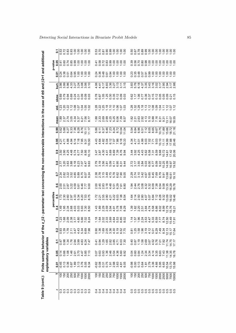
Detecting Social Interactions in Bivariate Probit Models 85T
ab
le 9
(co
nt.
):
rT
0.0
10.0
50.1
0.2
0.3
0.4
0.5
0.6
0.7
0.8
0.9
0.9
50.9
9m
ean
std
.skew
.ku
rt.
0.0
10.0
50.1
0.3
100
-0.45
0.14
0.47
0.93
1.23
1.49
1.73
2.00
2.34
2.77
3.50
4.21
5.62
1.89
1.23
0.69
3.96
0.24
0.41
0.53
0.3
150
0.13
0.66
0.98
1.39
1.68
1.95
2.30
2.51
2.82
3.20
3.90
4.71
5.88
2.37
1.20
0.79
3.99
0.38
0.60
0.72
0.3
200
0.36
1.08
1.34
1.78
2.09
2.34
2.60
2.87
3.22
3.63
4.25
4.88
6.27
2.74
1.22
0.94
5.96
0.51
0.74
0.83
0.3
250
0.87
1.46
1.76
2.11
2.38
2.68
2.97
3.22
3.52
3.88
4.48
4.94
6.33
3.05
1.12
0.69
4.33
0.64
0.85
0.93
0.3
500
1.89
2.61
2.94
3.47
3.77
4.03
4.33
4.59
4.85
5.18
5.74
6.14
7.38
4.34
1.08
0.24
3.27
0.95
0.99
1.00
0.3
750
3.13
3.70
3.99
4.43
4.80
5.03
5.34
5.61
5.89
6.23
6.77
7.18
8.28
5.37
1.07
0.31
3.24
1.00
1.00
1.00
0.3
1000
3.76
4.47
4.83
5.34
5.66
5.93
6.20
6.46
6.75
7.07
7.50
7.95
8.76
6.21
1.04
0.09
3.08
1.00
1.00
1.00
0.3
1500
5.05
5.85
6.24
6.69
7.02
7.30
7.53
7.77
8.07
8.47
8.95
9.31
10.11
7.56
1.05
0.09
3.06
1.00
1.00
1.00
0.3
2000
6.34
7.13
7.47
7.98
8.24
8.50
8.75
9.00
9.24
9.63
10.10
10.50
11.17
8.77
1.02
0.03
3.10
1.00
1.00
1.00
0.4
100
-0.62
0.07
0.41
0.90
1.18
1.43
1.72
2.00
2.38
2.79
3.47
4.43
5.86
1.88
1.28
0.78
4.06
0.24
0.41
0.53
0.4
150
0.08
0.63
0.94
1.36
1.64
1.89
2.21
2.45
2.78
3.19
3.87
4.64
6.11
2.33
1.22
0.87
4.41
0.36
0.58
0.70
0.4
200
0.31
0.93
1.29
1.69
2.02
2.29
2.55
2.83
3.15
3.56
4.30
4.82
6.37
2.69
1.25
1.05
6.17
0.48
0.72
0.81
0.4
250
0.75
1.36
1.65
2.05
2.33
2.59
2.90
3.18
3.49
3.81
4.41
5.04
6.46
2.99
1.18
1.25
8.83
0.61
0.83
0.90
0.4
500
1.91
2.46
2.82
3.36
3.69
3.94
4.21
4.48
4.75
5.09
5.69
6.12
7.23
4.25
1.10
0.30
3.36
0.94
0.99
0.99
0.4
750
2.98
3.54
3.85
4.30
4.64
4.91
5.22
5.51
5.78
6.11
6.69
7.07
8.24
5.25
1.10
0.35
3.27
1.00
1.00
1.00
0.4
1000
3.63
4.36
4.71
5.19
5.53
5.78
6.03
6.29
6.62
6.95
7.39
7.86
8.72
6.06
1.06
0.12
3.13
1.00
1.00
1.00
0.4
1500
4.81
5.60
6.03
6.52
6.85
7.08
7.38
7.61
7.90
8.31
8.76
9.18
10.04
7.39
1.07
0.09
3.11
1.00
1.00
1.00
0.4
2000
6.05
6.92
7.30
7.75
8.02
8.29
8.54
8.80
9.05
9.44
9.94
10.33
11.04
8.57
1.03
0.03
3.15
1.00
1.00
1.00
0.5
100
-0.98
0.04
0.40
0.81
1.14
1.39
1.64
1.94
2.29
2.72
3.44
4.34
5.54
1.82
1.28
0.62
3.83
0.23
0.39
0.50
0.5
150
0.00
0.60
0.87
1.25
1.57
1.82
2.14
2.44
2.74
3.17
3.92
4.77
6.84
2.31
1.32
1.17
5.76
0.35
0.56
0.67
0.5
200
0.13
0.84
1.19
1.58
1.96
2.20
2.50
2.76
3.10
3.55
4.25
5.01
6.96
2.63
1.28
1.06
6.18
0.48
0.70
0.78
0.5
250
0.64
1.24
1.58
1.96
2.24
2.51
2.80
3.08
3.42
3.84
4.43
4.99
6.51
2.92
1.18
0.77
4.37
0.57
0.80
0.89
0.5
500
1.81
2.34
2.69
3.19
3.53
3.84
4.07
4.32
4.67
5.03
5.62
6.03
7.12
4.13
1.13
0.36
3.35
0.91
0.98
0.99
0.5
750
2.79
3.34
3.67
4.12
4.47
4.74
5.07
5.32
5.65
6.00
6.58
7.02
8.05
5.10
1.12
0.37
3.43
0.99
1.00
1.00
0.5
1000
3.36
4.14
4.52
5.01
5.33
5.58
5.84
6.09
6.45
6.77
7.31
7.71
8.65
5.88
1.08
0.15
3.16
1.00
1.00
1.00
0.5
1500
4.66
5.35
5.76
6.29
6.59
6.86
7.12
7.38
7.69
8.09
8.59
9.03
9.67
7.16
1.09
0.12
3.02
1.00
1.00
1.00
0.5
2000
5.95
6.63
7.01
7.49
7.77
8.02
8.28
8.54
8.79
9.22
9.68
10.10
10.75
8.31
1.04
0.05
3.17
1.00
1.00
1.00
0.5
2500
6.65
7.43
7.92
8.34
8.74
8.99
9.32
9.58
9.91
10.25
10.72
11.11
11.89
9.31
1.11
0.05
2.95
1.00
1.00
1.00
0.5
5000
10.54
11.38
11.74
12.13
12.50
12.79
13.09
13.35
13.68
14.09
14.61
14.99
15.66
13.11
1.12
0.09
2.94
1.00
1.00
1.00
0.5
7500
13.70
14.35
14.75
15.17
15.49
15.76
16.02
16.29
16.61
16.97
17.42
17.88
18.72
16.07
1.07
0.21
3.17
1.00
1.00
1.00
0.5
10000
15.98
16.78
17.17
17.64
17.91
18.21
18.46
18.78
19.10
19.52
20.06
20.46
21.18
18.55
1.12
0.15
2.88
1.00
1.00
1.00
perc
en
tile
sp
-valu
e
Fin
ite s
am
ple
beh
avio
r o
f th
e z
_ 2 -
para
mete
r te
st
co
ncern
ing
th
e n
on
-ob
serv
ab
le i
nte
racti
on
s i
n t
he c
ase o
f r
0 a
nd
2=
1 a
nd
ad
dit
ion
al
exp
lan
ato
ry v
ari
ab
les