CAM Centre for Applied Microeconometrics Department of Economics University of Copenhagen http://www.econ.ku.dk/CAM/

Probit Models with Binary Endogenous Regressors

Jacob Nielsen Arendt and Anders Holm

2006-06

The activities of CAM are financed by a grant from The Danish National Research Foundation

Probit models with binary endogenous regressors

Jacob Nielsen Arendta and Anders Holmb

a Department of Business and Economics, University of Southern Denmark, Odense. email:

jna@sam.sdu.dk

bDepartment of Sociology, University of Copenhagen. email: anders.holm@sociology.ku.dk

February 2006 Abstract

Sample selection and endogeneity are frequent causes of biases in non-experimental empirical

studies. In binary models a standard solution involves complex multivariate models. A simple

approximation has been shown to work well in bivariate models. This paper extends the

approximation to a trivariate model. Simulations show that the approximation outperforms full

maximum likelihood while a least squares approximation may be severely biased. The methods

are used to estimate the influence of trust in the parliament and politicians on voting-

propensity. No previous studies have allowed for endogeneity of trust on voting and it is shown

to severely affect the results.

Keywords: Endogeneity; Multivariate Probit; Approximation; Monte Carlo Simulation

1. Introduction

In this paper we consider how to estimate the effect of endogenous binary variables in a binary

response model. This problem is of tremendous importance in most social sciences disciplines,

since these frequently rely on non-experimental data. It is well-known from especially linear

models that failing to take endogeneity into account may result in substantially biased results.

It is natural to assume that such bias extends to non-linear models (Yatchew and Griliches

(1985) derive the approximate bias in a probit model with continuous endogenous regressors).

We focus on models with qualititative variables for several reasons: 1) Less attention has been

paid to these models than when either dependent or independent endogenous variables are

continuous, 2) one frequently encounters qualitative variables in social sciences applications,

and 3) when both dependent and independent variables are qualitative correct modelling

require more complex models than if either is continuous. Specifically, simple two-stage

methods exist which account for endogeneity in models when either the dependent or the

independent endogenous variable is continuous (see e.g. Alvarez and Glasgow (2000) for a

comparison of methods in the latter case), whereas such procedures are generally not consistent

with qualitative endogenous variables. Although consistent estimates can be obtained by

multivariate modelling, this provides several difficulties both with respect to estimation and

with respect to making such models readily understandable to a wider audience. We, as a

consequence, think that it is of great value to consider simpler models that approximate the true

effects. We consider two types of approximations: a heckit-type and a least-squares type. These

are defined below.

For illustration we start by considering a binomial model with one endogenous binomial

explanatory variable and present the approximations to the full bivariate model. Nicoletti and

2

Perrachi (2001) consider how the heckit-approximation performs in a very similar case; a

binomial model with sample selection. The main contribution in this paper is to extend the

heckit-approximation to the case with two endogenous binomial explanatory variables and to

provide simulation results that illustrate the bias of this approximation as well as of a simpler

least-squares-based approximation in different settings. We find that the heckit approximation

works well and that it even outperforms full maximum likelihood estimation under serious

endogeneity in small samples. The least squares approximation works well under mild

endogeneity but may provide seriously biased estimates when endogeneity is severe. To

illustrate empirically how the approximation works we apply the heckit approximation for

estimation of the effect of political trust on voting behaviour. There is a substantial literature in

political sciences on this issue. Nevertheless, according to our knowledge, no previous studies

account for the potential endogeneity of trust on voting. We show that taking endogeneity into

account has important consequences for the estimated effect of trust on voting.

The paper is organized as follows: The next section presents the case with one endogenous

regressor. Section three extends the model to more endogenous or multinomial outcomes. In

section four, simulations ecidence for the estimators are presented. Section five presents the

empirical application on voting behaviour and section six presents some concluding remarks.

2. A model with one endogenous regression variable

In this section we present the case with two binary variables, and , where may have a

causal effects on , but where the variables are spuriously related due to observed as well as

unobserved independent variables. This situation is illustrated in the following fully parametric

model:

1y 2y 2y

1y

3

(1) 1 2 1 1 1

2 2 2 2

1 2 1 2

1( 0),1( 0),

( , | , ) ~ (0,0,1,1, ),

y y xy x

x x N

α β εβ ε

ε ε ρ

= + + >= + >

where1( is the indicator function taking the value one if the statement in the brackets are true

and zero otherwise.

.)

1 2, ,α β β are regression coefficients, (.,.,.,., )N ρ indicates the standard

bivariate normal distribution with correlation coefficients ρ . When ρ is zero the model for y1

is the standard probit model.1

Basically, the model states three reasons why we might observe and to be correlated: 1) a

causal relation due to the influence from on through the parameter

1y 2y

2y 1y α , 2) and may

depend on correlated observed variables (the x’s) and 3) and may depend on correlated

unobserved variables (the ε’s).

2y 1y

2y 1y

Consistent and asymptotically efficient parameter estimates are obtained by maximum

likelihood estimation of the bivariate probit model. This is based on a likelihood function

consisting of a product of individual contributions of the type:

(1) 1 2 1 2 1 2 1 2 1 2 1 2 1 2 2( , , | , , , ) ( , | , ) ( | , ) ( | ).i i i i i i i i i i i i i iL y y x x P y y x x P y y x P y xα β β = =

1 We stress an important difference between the multivariate probit model and log-linear models. The latter were

considered by Nerlove and Press (1976) and discussed by Heckman (1978) among others. In these models, the

bivariate probability of y1 and y2 can be defined as: 1 2 0 1 1 2 2 12 1 2( , ) exp( ) /P y y y y y y Dα α α α= + + + , where D is the

appropriate weight. In this model, y1 and y2 are independent if and only if α12 is zero. Therefore, it only has one

parameter describing the relation between y1 and y2 in contrast to the multivariate probit model which for two

types of relations: structural ( 0α ≠ ) and spurious ( 0ρ ≠ ), and therefore allows for causal interpretations.

4

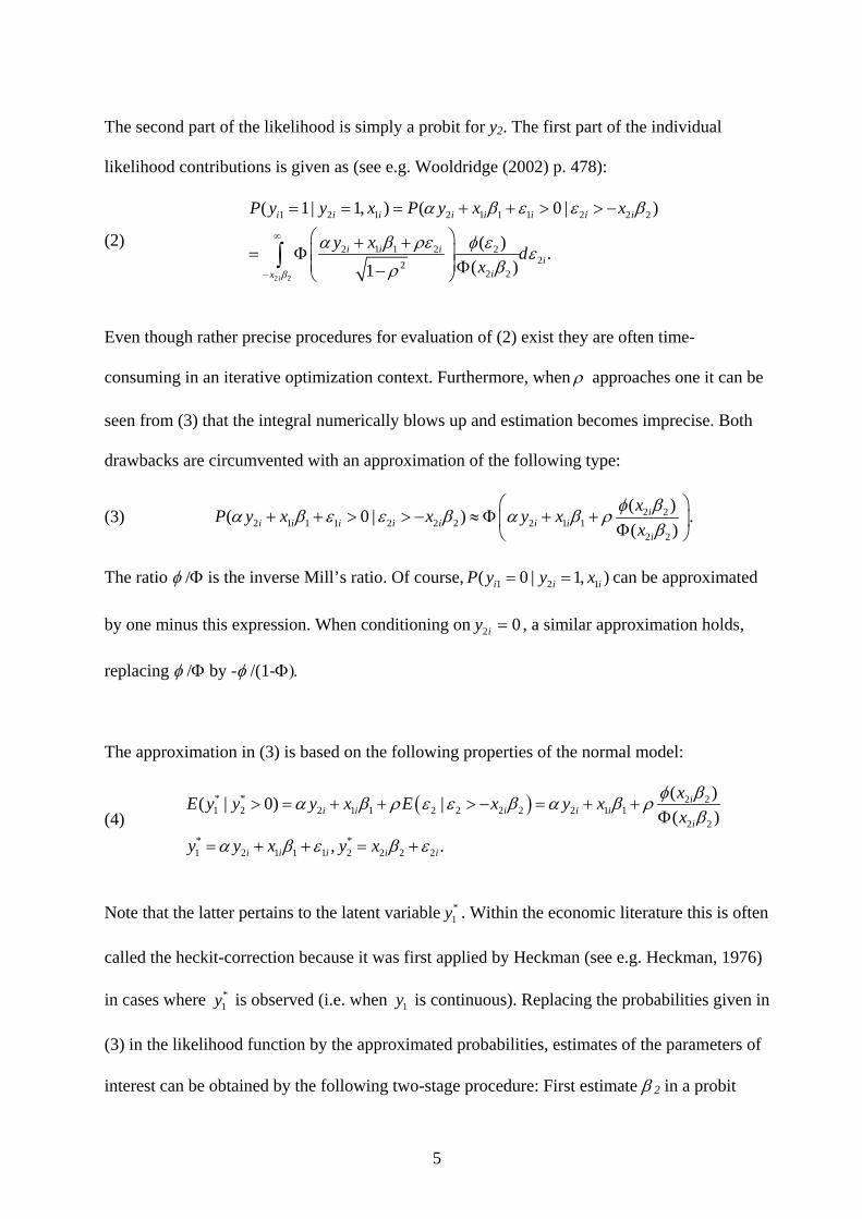
The second part of the likelihood is simply a probit for y2. The first part of the individual

likelihood contributions is given as (see e.g. Wooldridge (2002) p. 478):

(2)

2 2

1 2 1 2 1 1 1 2 2

2 1 1 2 222

2 2

( 1| 1, ) ( 0 |

( ) .( )1i

i i i i i i i i

i i ii

ix

P y y x P y x x

y x dxβ

2 )α β ε ε β

α β ρε φ ε εβρ

∞

−

= = = + + > > −

⎛ ⎞+ +⎜ ⎟= Φ⎜ ⎟ Φ−⎝ ⎠

∫

Even though rather precise procedures for evaluation of (2) exist they are often time-

consuming in an iterative optimization context. Furthermore, when ρ approaches one it can be

seen from (3) that the integral numerically blows up and estimation becomes imprecise. Both

drawbacks are circumvented with an approximation of the following type:

(3) 2 22 1 1 1 2 2 2 2 1 1

2 2

( )( 0 | )( )

ii i i i i i i

i

xP y x x y xx

φ βα β ε ε β α β ρβ

⎛ ⎞+ + > > − ≈ Φ + +⎜ ⎟Φ⎝ ⎠

.

1 )i

The ratio φ /Φ is the inverse Mill’s ratio. Of course, 1 2( 0 | 1,i iP y y x= = can be approximated

by one minus this expression. When conditioning on 2 0iy = , a similar approximation holds,

replacing φ /Φ by -φ /(1-Φ).

The approximation in (3) is based on the following properties of the normal model:

(4) ( )* * 2 2

1 2 2 1 1 2 2 2 2 2 1 12 2

* *1 2 1 1 1 2 2 2 2

( )( | 0) |( )

, .

ii i i i i

i

i i i i i

xE y y y x E x y xx

y y x y x

φ βα β ρ ε ε β α β ρβ

α β ε β ε

> = + + > − = + +Φ

= + + = +

Note that the latter pertains to the latent variable . Within the economic literature this is often

called the heckit-correction because it was first applied by Heckman (see e.g. Heckman, 1976)

in cases where is observed (i.e. when is continuous). Replacing the probabilities given in

(3) in the likelihood function by the approximated probabilities, estimates of the parameters of

interest can be obtained by the following two-stage procedure: First estimate β

*1y

*1y 1y

2 in a probit

5

model for . Then calculate the correction factors and estimate (α, β2y 1, ρ) in a probit model

with the correction factor as additional explanatory variables.

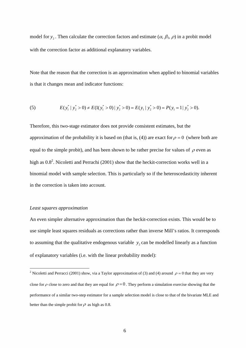
Note that the reason that the correction is an approximation when applied to binomial variables

is that it changes mean and indicator functions:

(5) * * * * * *1 2 1 2 1 2 1 2( | 0) (1( 0) | 0) ( | 0) ( 1| 0).E y y E y y E y y P y y> ≠ > > = > = = >

Therefore, this two-stage estimator does not provide consistent estimates, but the

approximation of the probability it is based on (that is, (4)) are exact for 0ρ = (where both are

equal to the simple probit), and has been shown to be rather precise for values of ρ even as

high as 0.82. Nicoletti and Perrachi (2001) show that the heckit-correction works well in a

binomial model with sample selection. This is particularly so if the heteroscedasticity inherent

in the correction is taken into account.

Least squares approximation

An even simpler alternative approximation than the heckit-correction exists. This would be to

use simple least squares residuals as corrections rather than inverse Mill’s ratios. It corresponds

to assuming that the qualitative endogenous variable can be modelled linearly as a function

of explanatory variables (i.e. with the linear probability model):

2y

2 Nicoletti and Perracci (2001) show, via a Taylor approximation of (3) and (4) around 0ρ = that they are very

close for ρ close to zero and that they are equal for 0ρ = . They perform a simulation exercise showing that the

performance of a similar two-step estimator for a sample selection model is close to that of the bivariate MLE and

better than the simple probit for ρ as high as 0.8.

6

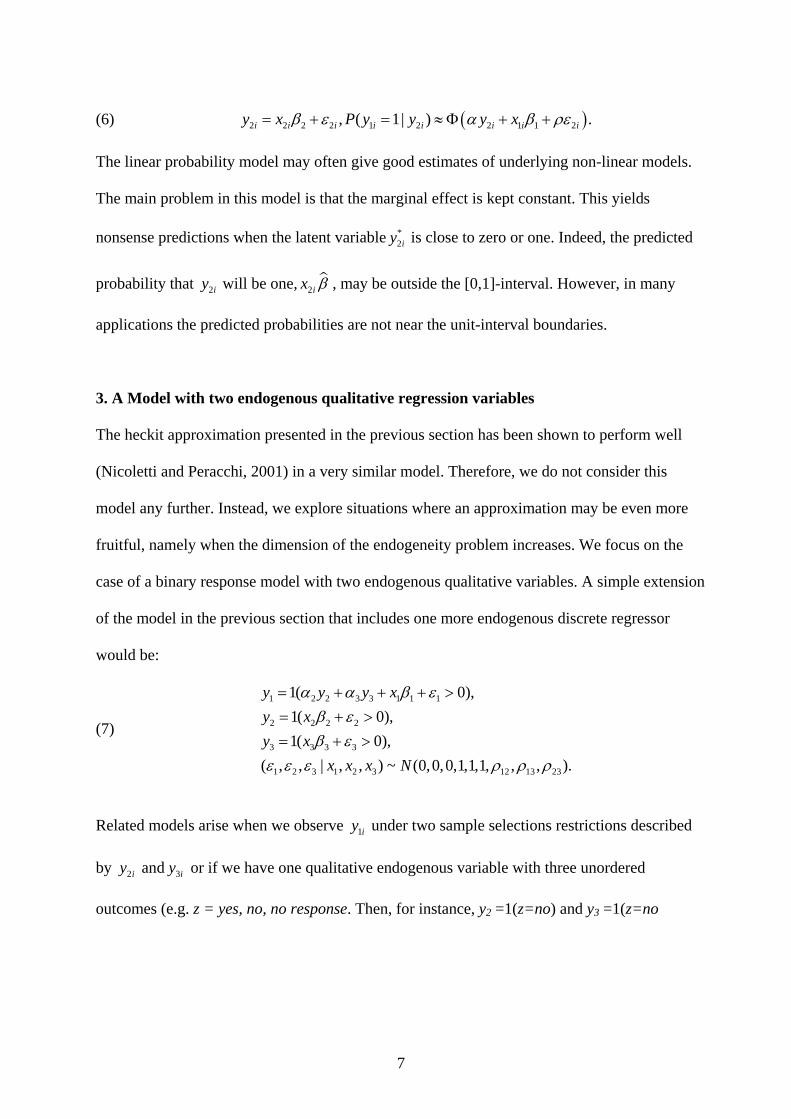
(6) ( )2 2 2 2 1 2 2 1 1 2, ( 1| ) .i i i i i i i iy x P y y y xβ ε α= + = ≈ Φ + +β ρε

The linear probability model may often give good estimates of underlying non-linear models.

The main problem in this model is that the marginal effect is kept constant. This yields

nonsense predictions when the latent variable is close to zero or one. Indeed, the predicted

probability that will be one,

*2iy

2iy 2ix β , may be outside the [0,1]-interval. However, in many

applications the predicted probabilities are not near the unit-interval boundaries.

3. A Model with two endogenous qualitative regression variables

The heckit approximation presented in the previous section has been shown to perform well

(Nicoletti and Peracchi, 2001) in a very similar model. Therefore, we do not consider this

model any further. Instead, we explore situations where an approximation may be even more

fruitful, namely when the dimension of the endogeneity problem increases. We focus on the

case of a binary response model with two endogenous qualitative variables. A simple extension

of the model in the previous section that includes one more endogenous discrete regressor

would be:

(7)

1 2 2 3 3 1 1 1

2 2 2 2

3 3 3 3

1 2 3 1 2 3 12 13 23

1( 0),1( 0),1( 0),

( , , | , , ) ~ (0,0,0,1,1,1, , , ).

y y y xy xy x

x x x N

α α β εβ εβ ε

ε ε ε ρ ρ ρ

= + + + >= + >= + >

Related models arise when we observe under two sample selections restrictions described

by or if we have one qualitative endogenous variable with three unordered

outcomes (e.g. z = yes, no, no response. Then, for instance, y

1iy

2 and iy 3iy

2 =1(z=no) and y3 =1(z=no

7

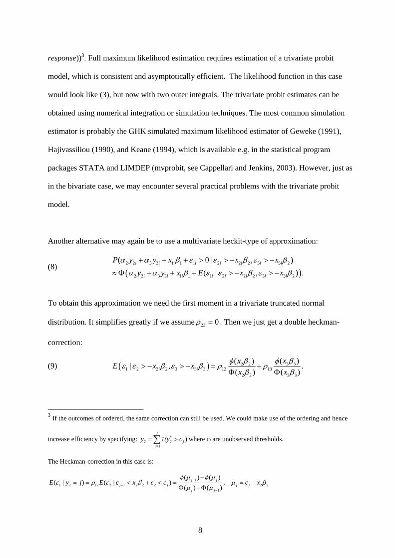
response))3. Full maximum likelihood estimation requires estimation of a trivariate probit

model, which is consistent and asymptotically efficient. The likelihood function in this case

would look like (3), but now with two outer integrals. The trivariate probit estimates can be

obtained using numerical integration or simulation techniques. The most common simulation

estimator is probably the GHK simulated maximum likelihood estimator of Geweke (1991),

Hajivassiliou (1990), and Keane (1994), which is available e.g. in the statistical program

packages STATA and LIMDEP (mvprobit, see Cappellari and Jenkins, 2003). However, just as

in the bivariate case, we may encounter several practical problems with the trivariate probit

model.

Another alternative may again be to use a multivariate heckit-type of approximation:

(8) ( )2 2 3 3 1 1 1 2 2 2 3 3 2

2 2 3 3 1 1 1 2 2 2 3 3 2

( 0 | ,( | , )

i i i i i i i i

i i i i i i i i

P y y x x xy y x E x x

).

α α β ε ε β ε βα α β ε ε β ε β

+ + + > > − > −

≈ Φ + + + > − > −

To obtain this approximation we need the first moment in a trivariate truncated normal

distribution. It simplifies greatly if we assume 23 0ρ = . Then we just get a double heckman-

correction:

(9) ( ) 3 32 21 2 2 2 3 3 3 12 13

2 2 3 3

( )( )| ,( ) ( )i i

xxE x xx x

.φ βφ βε ε β ε β ρ ρβ β

> − > − = +Φ Φ

j

3 If the outcomes of ordered, the same correction can still be used. We could make use of the ordering and hence

increase efficiency by specifying: where c)J

*2 2

j=1y 1(y c= >∑ j are unobserved thresholds.

The Heckman-correction in this case is:

11 2 12 2 1 2 2 2 2 2

1

( ) ( )( | ) ( | ) ,

( ) ( )j j

j j jj j

E y j E c x c c xφ µ φ µ

jε ρ ε β ε µ βµ µ

−−

−

−= = < + < = = −

Φ − Φ

8

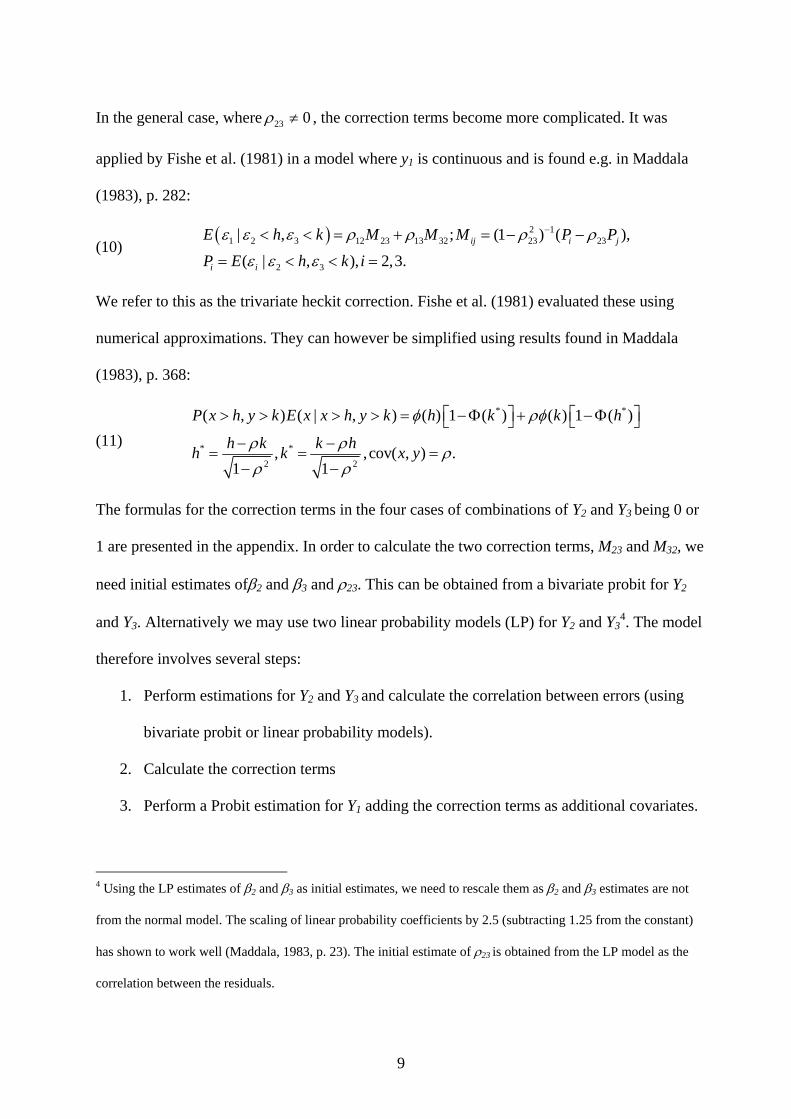
In the general case, where 23 0ρ ≠ , the correction terms become more complicated. It was

applied by Fishe et al. (1981) in a model where y1 is continuous and is found e.g. in Maddala

(1983), p. 282:

(10) ( ) 2 1

1 2 3 12 23 13 32 23 23

2 3

| , ; (1 ) (

( | , ), 2,3.ij i j

i i

),E h k M M M P P

P E h k i

ε ε ε ρ ρ ρ ρ

ε ε ε

−< < = + = − −

= < < =

We refer to this as the trivariate heckit correction. Fishe et al. (1981) evaluated these using

numerical approximations. They can however be simplified using results found in Maddala

(1983), p. 368:

(11)

* *

* *

2 2

( , ) ( | , ) ( ) 1 ( ) ( ) 1 ( )

, , cov( , ) .1 1

P x h y k E x x h y k h k k h

h k k hh k x y

φ ρφ

ρ ρ ρρ ρ

⎡ ⎤ ⎡> > > > = − Φ + − Φ ⎤⎣ ⎦ ⎣− −

= = =− −

⎦

The formulas for the correction terms in the four cases of combinations of Y2 and Y3 being 0 or

1 are presented in the appendix. In order to calculate the two correction terms, M23 and M32, we

need initial estimates ofβ2 and β3 and ρ23. This can be obtained from a bivariate probit for Y2

and Y3. Alternatively we may use two linear probability models (LP) for Y2 and Y34. The model

therefore involves several steps:

1. Perform estimations for Y2 and Y3 and calculate the correlation between errors (using

bivariate probit or linear probability models).

2. Calculate the correction terms

3. Perform a Probit estimation for Y1 adding the correction terms as additional covariates.

4 Using the LP estimates of β2 and β3 as initial estimates, we need to rescale them as β2 and β3 estimates are not

from the normal model. The scaling of linear probability coefficients by 2.5 (subtracting 1.25 from the constant)

has shown to work well (Maddala, 1983, p. 23). The initial estimate of ρ23 is obtained from the LP model as the

correlation between the residuals.

9

We have considered whether the performance of the heckit approximation improved if we take

into account that it is heteroscedastic. Recall that Nicoletti and Peracchi (2001) found this to be

useful in the case with one endogenous regressor. However, as opposed to Nicoletti and

Peracchi (2001) we did not find much gain from heteroscedasticity corrections. The formula

for the variance needed for heteroscedasticity correction is available from the authors upon

request.

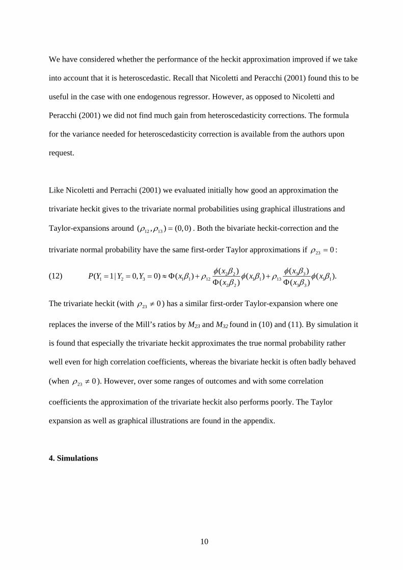
Like Nicoletti and Perrachi (2001) we evaluated initially how good an approximation the

trivariate heckit gives to the trivariate normal probabilities using graphical illustrations and

Taylor-expansions around 12 13( , ) (0,0)ρ ρ = . Both the bivariate heckit-correction and the

trivariate normal probability have the same first-order Taylor approximations if 23 0ρ = :

(12) 3 32 21 2 3 1 1 12 1 1 13 1 1

2 2 3 3

( )( )( 1| 0, 0) ( ) ( ) (( ) ( )

xxP Y Y Y x x xx x

).φ βφ ββ ρ φ β ρ φβ β

= = = ≈ Φ + +Φ Φ

β

The trivariate heckit (with 23 0ρ ≠ ) has a similar first-order Taylor-expansion where one

replaces the inverse of the Mill’s ratios by M23 and M32 found in (10) and (11). By simulation it

is found that especially the trivariate heckit approximates the true normal probability rather

well even for high correlation coefficients, whereas the bivariate heckit is often badly behaved

(when 23 0ρ ≠ ). However, over some ranges of outcomes and with some correlation

coefficients the approximation of the trivariate heckit also performs poorly. The Taylor

expansion as well as graphical illustrations are found in the appendix.

4. Simulations

10

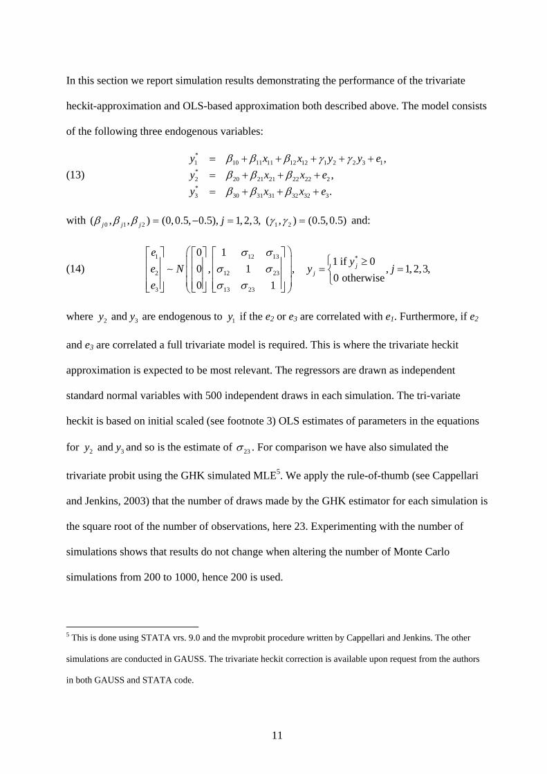
In this section we report simulation results demonstrating the performance of the trivariate

heckit-approximation and OLS-based approximation both described above. The model consists

of the following three endogenous variables:

(13)

*1 10 11 11 12 12 1 2 2 3*2 20 21 21 22 22 2*3 30 31 31 32 32 3

,,.

y x x yy x x ey x x e

β β β γ γβ β ββ β β

= + + + + += + + += + + +

1y e

with 0 1 2 1 2( , , ) (0,0.5, 0.5), 1, 2,3, ( , ) (0.5,0.5)j j j jβ β β γ γ= − = = and:

(14) 1 12 13 *

2 12 23

3 13 23

0 11 if 0

0 , 1 , , 1, 2,3,0 otherwise

0 1

jj

ey

e N y je

σ σσ σσ σ

⎛ ⎞⎡ ⎤ ⎡ ⎤ ⎡ ⎤⎧ ≥⎜ ⎟⎢ ⎥ ⎢ ⎥ ⎢ ⎥ = =⎨⎜ ⎟⎢ ⎥ ⎢ ⎥ ⎢ ⎥ ⎩⎜ ⎟⎢ ⎥ ⎢ ⎥ ⎢ ⎥⎣ ⎦ ⎣ ⎦ ⎣ ⎦⎝ ⎠

∼

where are endogenous to if the e2 and y 3y

3y

1y 2 or e3 are correlated with e1. Furthermore, if e2

and e3 are correlated a full trivariate model is required. This is where the trivariate heckit

approximation is expected to be most relevant. The regressors are drawn as independent

standard normal variables with 500 independent draws in each simulation. The tri-variate

heckit is based on initial scaled (see footnote 3) OLS estimates of parameters in the equations

for and so is the estimate of 2 and y 23σ . For comparison we have also simulated the

trivariate probit using the GHK simulated MLE5. We apply the rule-of-thumb (see Cappellari

and Jenkins, 2003) that the number of draws made by the GHK estimator for each simulation is

the square root of the number of observations, here 23. Experimenting with the number of

simulations shows that results do not change when altering the number of Monte Carlo

simulations from 200 to 1000, hence 200 is used.

5 This is done using STATA vrs. 9.0 and the mvprobit procedure written by Cappellari and Jenkins. The other

simulations are conducted in GAUSS. The trivariate heckit correction is available upon request from the authors

in both GAUSS and STATA code.

11

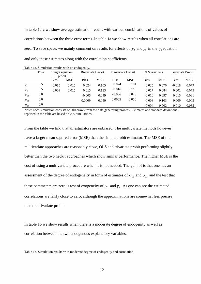
In table 1a-c we show average estimation results with various combinations of values of

correlations between the three error terms. In table 1a we show results when all correlations are

zero. To save space, we mainly comment on results for effects of in the equation

and only these estimates along with the correlation coefficients.

2 and y 3y 1y

Table 1a. Simulation results with no endogenity. True Single equation

probit Bi-variate Heckit Tri-variate Heckit OLS residuals Trivariate Probit

Bias MSE Bias MSE Bias MSE Bias MSE Bias MSE 1γ 0.5 0.015 0.015 0.024 0.105 0.024 0.104 0.025 0.076 -0.018 0.079 2γ 0.5 0.009 0.015 0.015 0.113 0.016 0.113 0.017 0.084 0.001 0.075 12σ 0.0 -0.005 0.049 -0.006 0.048 -0.010 0.097 0.015 0.031

0.0 0.0009 0.050 0.0005 0.050 -0.003 0.103 0.009 0.005 13σ

23σ 0.0 -0.004 0.002 0.010 0.035 Note: Each simulation consists of 500 draws from the data generating process. Estimates and standard deviations reported in the table are based on 200 simulations.

From the table we find that all estimators are unbiased. The multivariate methods however

have a larger mean squared error (MSE) than the simple probit estimator. The MSE of the

multivariate approaches are reasonably close, OLS and trivariate probit performing slightly

better than the two heckit approaches which show similar performance. The higher MSE is the

cost of using a multivariate procedure when it is not needed. The gain of is that one has an

assessment of the degree of endogeneity in form of estimates of 12 13and σ σ and the test that

these parameters are zero is test of exogeneity of . As one can see the estimated

correlations are fairly close to zero, although the approximations are somewhat less precise

than the trivariate probit.

2 and y 3y

In table 1b we show results when there is a moderate degree of endogenity as well as

correlation between the two endogenous explanatory variables.

Table 1b. Simulation results with moderate degree of endogenity and correlation

12

between endogenous explanatory variables. True Single equation

probit Bi-variate Heckit Tri-variate Heckit OLS residuals Trivariate Probit

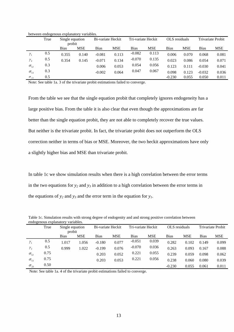
Bias MSE Bias MSE Bias MSE Bias MSE Bias MSE 1γ 0.5 0.355 0.140 -0.081 0.113 -0.082 0.113 0.006 0.070 0.068 0.081 2γ 0.5 0.354 0.145 -0.071 0.134 -0.070 0.135 0.023 0.086 0.054 0.071 12σ 0.3 0.006 0.053 0.054 0.056 0.123 0.111 -0.030 0.041

0.3 -0.002 0.064 0.047 0.067 0.098 0.123 -0.032 0.036 13σ23σ 0.5 -0.230 0.055 0.050 0.011

Note: See table 1a. 3 of the trivariate probit estimations failed to converge.

From the table we see that the single equation probit that completely ignores endogeneity has a

large positive bias. From the table it is also clear that even though the approximations are far

better than the single equation probit, they are not able to completely recover the true values.

But neither is the trivariate probit. In fact, the trivariate probit does not outperform the OLS

correction neither in terms of bias or MSE. Moreover, the two heckit approximations have only

a slightly higher bias and MSE than trivariate probit.

In table 1c we show simulation results when there is a high correlation between the error terms

in the two equations for y2 and y3 in addition to a high correlation between the error terms in

the equations of y2 and y3 and the error term in the equation for y1.

Table 1c. Simulation results with strong degree of endogenity and and strong positive correlation between endogenous explanatory variables. True Single equation

probit Bi-variate Heckit Tri-variate Heckit OLS residuals Trivariate Probit

Bias MSE Bias MSE Bias MSE Bias MSE Bias MSE 1γ 0.5 1.017 1.056 -0.180 0.077 -0.051 0.039 0.282 0.102 0.149 0.099 2γ 0.5 0.999 1.022 -0.199 0.076 -0.070 0.036 0.263 0.093 0.167 0.088 12σ 0.75 0.203 0.052 0.221 0.055 0.239 0.059 0.098 0.062

0.75 0.203 0.053 0.221 0.056 0.238 0.060 0.080 0.039 13σ

23σ 0.50 -0.230 0.055 0.061 0.011 Note: See table 1a. 4 of the trivariate probit estimations failed to converge.

13

From the table we again find a large bias for the two endogenous explanatory variables in the

single equation probit model. The bias of the trivariate heckit is relatively low whereas all the

three other multivariate methods have a non-negligible bias, including the trivariate probit and

the OLS-correction. The trivariate heckit also outperforms the other estimators in terms of

MSE. The correlation coefficients are however biased for the approximations while far closer

to the true values for the trivariate probit.

We have made simulations for a model with very similar true values as in table 1c, except that

the correlation of the error term in the equation of y3 and the two other error terms are negative.

The findings from this exercise are similar to findings in table 1c. The caveat in this simulation

is that under certain parameterizations the probit does not even get the sign right for the

coefficient for y3.

Finally, it is worth noting that in all simulations the estimated coefficients for the exogenous

explanatory variables (except the constant term) seem to be well-estimated in the single

equation probit model, irrespective of the severity of the endogenity of y2 and y3. This is

surprising and may be due to the fact that all regressors are assumed different and uncorrelated.

An application of voting and trust

In this section we use an empirical application to illustrate how endogeneity of binomial

indicators in binomial models may affect the estimated effects. The empirical example is a

study of the effect of trust on voting behaviour.

14

There are several examples in the literature seeking to estimate the effect of trust on voting

behaviour. In Pattie and Johnston (2001), voting in the 1997 election in the UK is analysed

using both trust indices and previous voting behaviour as explanatory variables. In Peterson

and Wrighton (1998) voting at the four previous US presidential elections is analysed also

using trust, through the trust in government index from Miller (1974), on voting behaviour at

the US presidential elections. Cox (2003) analyses voter turn out at European parliament

elections using a variety of trust measures. All these studies treat trust as exogenous. However,

one can imagine several reasons why this assumption may fail.

First of all, since voting behaviour is often reported as voting in the latest election (which is

also the case in our application), there might be a problem of reverse causality. Information

obtained since the last election about how the current politicians and parliament have

performed, might affect the responses on trust in politicians and the parliament. Second, trust is

a subjective measure, and might thus be contaminated by substantial measurement error, which

also make trust an endogenous variable. Finally, spurious relations (unobserved heterogeneity)

might in general make trust variables endogenous. For example, people who have a general

positive attitude are more likely to vote as well as being more likely to trust other, leaving

attitude out of the model will induce a spurious relationship between voting and trust. In some

studies on voting behaviour the trust variables are viewed as indicators of social capital (e.g.

Cox, 2003). If social capital is the reason why trust and voting are related, it is likely that social

capital is not fully described by trust, and hence a host of other indicators may be correlated

with voting behaviour. However, if other dimensions of social capital relevant to voting

behaviour, while not being included in the model, are also related to trust they are swept into

the error term and will induce endogeneity of the trust variables.

15

None of the mentioned studies acknowledge the potential endogeneity of the trust variables.

An exception is the related case studied by Alvarez and Glasgow (2000), who consider how

voter uncertainty on the political candidate’s policy position affects voting behaviour. They

take endogeneity into account but use a continuous measure of voter uncertainty, thus they

consider another class of estimators than the ones described here.

In our application we show that endogenity is a serious problem and whether it is taken into

account or not has serious implications for the results obtained. To encompass our application

to the methods of several binary endogenous variables, we use two trust variables; namely trust

in politicians and trust in the parliament.

In our exampled the response variable (y1 in (1)) is whether the respondent voted in the last

national election. The endogenous variable (y2 in (1)) is whether the respondent has trust in the

national parliament. Data comes from the European social survey (ESS), see

http://www.europeansocialsurvey.org/ for further documentation on the data. We have sampled

3,651 randomly cases among eligible voters only in all countries in the ESS. However, we

exclude a country indicator as, in preliminary analysis, it turned out that although significant

on vote, the exclusion of this variable did not affect the estimate of trust on voting behaviour,

and hence we feel justified to leave it out of the model for simplicity.

In table 2, we show summary statistics for our sample.

16

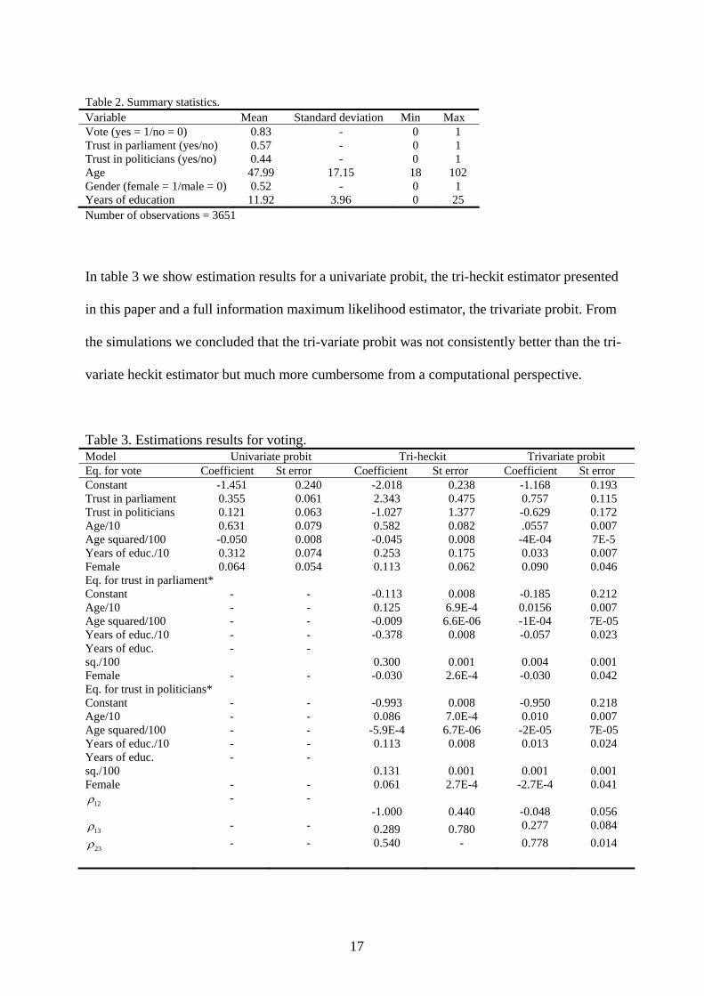
Table 2. Summary statistics. Variable Mean Standard deviation Min Max Vote (yes = 1/no = 0) 0.83 - 0 1 Trust in parliament (yes/no) 0.57 - 0 1 Trust in politicians (yes/no) 0.44 - 0 1 Age 47.99 17.15 18 102 Gender (female = 1/male = 0) 0.52 - 0 1 Years of education 11.92 3.96 0 25 Number of observations = 3651

In table 3 we show estimation results for a univariate probit, the tri-heckit estimator presented

in this paper and a full information maximum likelihood estimator, the trivariate probit. From

the simulations we concluded that the tri-variate probit was not consistently better than the tri-

variate heckit estimator but much more cumbersome from a computational perspective.

Table 3. Estimations results for voting. Model Univariate probit Tri-heckit Trivariate probit Eq. for vote Coefficient St error Coefficient St error Coefficient St error Constant -1.451 0.240 -2.018 0.238 -1.168 0.193 Trust in parliament 0.355 0.061 2.343 0.475 0.757 0.115 Trust in politicians 0.121 0.063 -1.027 1.377 -0.629 0.172 Age/10 0.631 0.079 0.582 0.082 .0557 0.007 Age squared/100 -0.050 0.008 -0.045 0.008 -4E-04 7E-5 Years of educ./10 0.312 0.074 0.253 0.175 0.033 0.007 Female 0.064 0.054 0.113 0.062 0.090 0.046 Eq. for trust in parliament* Constant - - -0.113 0.008 -0.185 0.212 Age/10 - - 0.125 6.9E-4 0.0156 0.007 Age squared/100 - - -0.009 6.6E-06 -1E-04 7E-05 Years of educ./10 - - -0.378 0.008 -0.057 0.023 Years of educ. sq./100

- - 0.300 0.001

0.004

0.001

Female - - -0.030 2.6E-4 -0.030 0.042 Eq. for trust in politicians* Constant - - -0.993 0.008 -0.950 0.218 Age/10 - - 0.086 7.0E-4 0.010 0.007 Age squared/100 - - -5.9E-4 6.7E-06 -2E-05 7E-05 Years of educ./10 - - 0.113 0.008 0.013 0.024 Years of educ. sq./100

- - 0.131 0.001

0.001

0.001

Female - - 0.061 2.7E-4 -2.7E-4 0.041 12ρ - -

-1.000 0.440

-0.048

0.056 13ρ - - 0.289 0.780 0.277 0.084

23ρ - - 0.540 - 0.778 0.014

17

Note: *For the Tri-heckit model, these are the re-scaled OLS regression coefficients and the estimate of 23ρ is the correlation between the OLS residuals. Based on 3651 observations.

From the table we find that both trust in the parliament and trust in the politicians increases the

likelihood of voting in the univariate probit. However, both the trivariate heckit as well as the

trivariate probit agrees that only trust in the parliament increases the likelihood of voting,

whereas trust in the politicians decreases the likelihood of voting. Hence, it appears that the

univariate probit completely misses the qualitative relationship between trust in politicians and

voting. It appears from all models, with varying effect and significance, that if the electorate

trusts the institutional set up of representative democracy they are more likely to vote. This

makes sense: If you believe in the system, you are more likely to use it. However, the

univariate probit completely disagrees with the two other models on the impact of trust in

politicians. But the negative relationship between trust in politicians and voting, predicted by

both the tri-variate heckit as well as the trivarite probit, also makes sense: If you have trust in

the politicians you are likely to gain less from voting than if you do not trust them. Therefore,

if you do not trust politicians you have a higher incentive to vote in order to change the

composition of the parliament.

From the table we find evidence of spurious correlation between trust and voting: the error

terms between voting and trust in parliament (ρ12) are negatively correlated (only significant in

the tri-heckit) and the error terms between trust in the politicians and voting (ρ13) are positively

correlated (only significant in the trivariate probit). Finally, the error terms between trust in the

parliament and politicians are positively correlated (ρ23).

18

Ignoring these correlations, as in the single equation probit, implies that trust in parliament and

trust in politicians captures both the causal effect of the trust indicators on voting as well as a

spurious effect between voting and trust. For trust in politicians it turns out that the positive

spurious relation outweighs the negative causal effect, producing a positive estimate in the

simple probit model. For trust in the parliament the negative spurious relation with voting

implies that the single equation probit model greatly underestimate the causal effect of trust in

the parliament.

5. Conclusion

We have introduced an approximation of a binomial normal model with two binomial

endogenous regressors as an alternative to the more complex trivariate probit model. We

considered the small sample properties of the approximation and of a simple OLS-based

approximation. We showed that a standard probit model that does not account for endogeneity

is severely biased in the presence of even moderate endogeneity. The approximations are less

biased. This is particularly so for the heckit approximation when the degree of endogeneity is

severe. In the latter case, the bias of both the OLS-based approximation and the trivariate

probit are not neglible and the efficiency loss of both approximations compared to the standard

probit is small. From our application we show both the importance of taking into account

endogeneity of binary variables and that the trivarite heckit estimator is a useful tool for doing

so. When ignoring endogenity one gets very different estimates compares to what is obtained

from models that corrects for endogenity. In certain cases one even gets different signs of the

effects of the endogenous variables.

Acknowledgements

19

We would like to thank Mads Meier Jæger and participants at the 28th Symposium for Applied

Statistics in Copenhagen, 2006, for useful comments.

References

Alvarez, R. M. and G. Glagow, (2000). Two-Stage Estimation of Nonrecursive Choice Models.

Political Analysis 8 (2), 11:24.

Cappellari, L. and S. P. Jenkins (2003). Multivariate probit regression using simulated

maximum likelihood. Stata Journal 3 (3), 278-294.

Cox, M. (2003). When trust matters: explaining differences in voter turnout, Journal of

Common Market Studies, 41 (4), 757-70.

Fishe, R. P. H., R. P. Trost and P. Lurie (1981). Labor force earnings and college choice of

young women: An examination of selectivity bias and comparative advantage. Economics of

Education Review 1 (2), 169-191.

Geweke, J. (1991). Efficient Simulation from the Multivariate Normal and Student-t

Distributions Subject to Linear Constraints, Computer Science and Statistics: Proceedings of

the Twenty-Third Symposium on the Interface, 571-578.

Hajivassiliou, V. (1990). Smooth Simulation Estimation of Panel Data LDV Models.

Unpublished Manuscript.

20

Heckman, J. J. (1976). The common structure of statistical models of truncation, sample

selection and limited dependent variables and a simple estimator for such models. Annals of

Economic and Social Measurement 15, 475-492.

Heckman, J. J. (1978). Dummy endogenous variables in a simultaneous equation system.

Econometrica 46 (6), 931-959.

Keane, M. P. (1994). A Computationally Practical Simulation Estimator for Panel Data,

Econometrica, 62(1), 95-116.

Nicoletti, C. and F. Peracchi (2001) Two-step estimation of binary response models with

sample selection, unpublished working paper.

Maddala, G. S. (1983). Limited-Dependent and Qualitative Variables in Econometrics.

Econometric Society Monographs. Cambridge University Press.

Miller, A.H. (1974). Political issues and trust in government: 1964-1970. American Political

Science Review 68: 951-972.

Pattie, C. and R. Johnston (2001) “Losing the voters’ trust: evaluations of the political system

and voting at the 1997 British general election”, British Journal of Politics and International

Relations 3 (2), 191-222.

21

Peterson, Geoff and J. Mark Wrighton (1998) “Expressions of Distrust: Third party voting and

Cynicism in Government”. Unpublished working paper.

Wooldridge, J. M. (2002). Econometric Analysis of Cross Section and Panel Data. Cambridge

MA: MIT Press.

Yatchew, A. and Z. Griliches (1985). Specification Error in Probit Models. The Review of

Economics and Statistics 67 (1), 134-139.

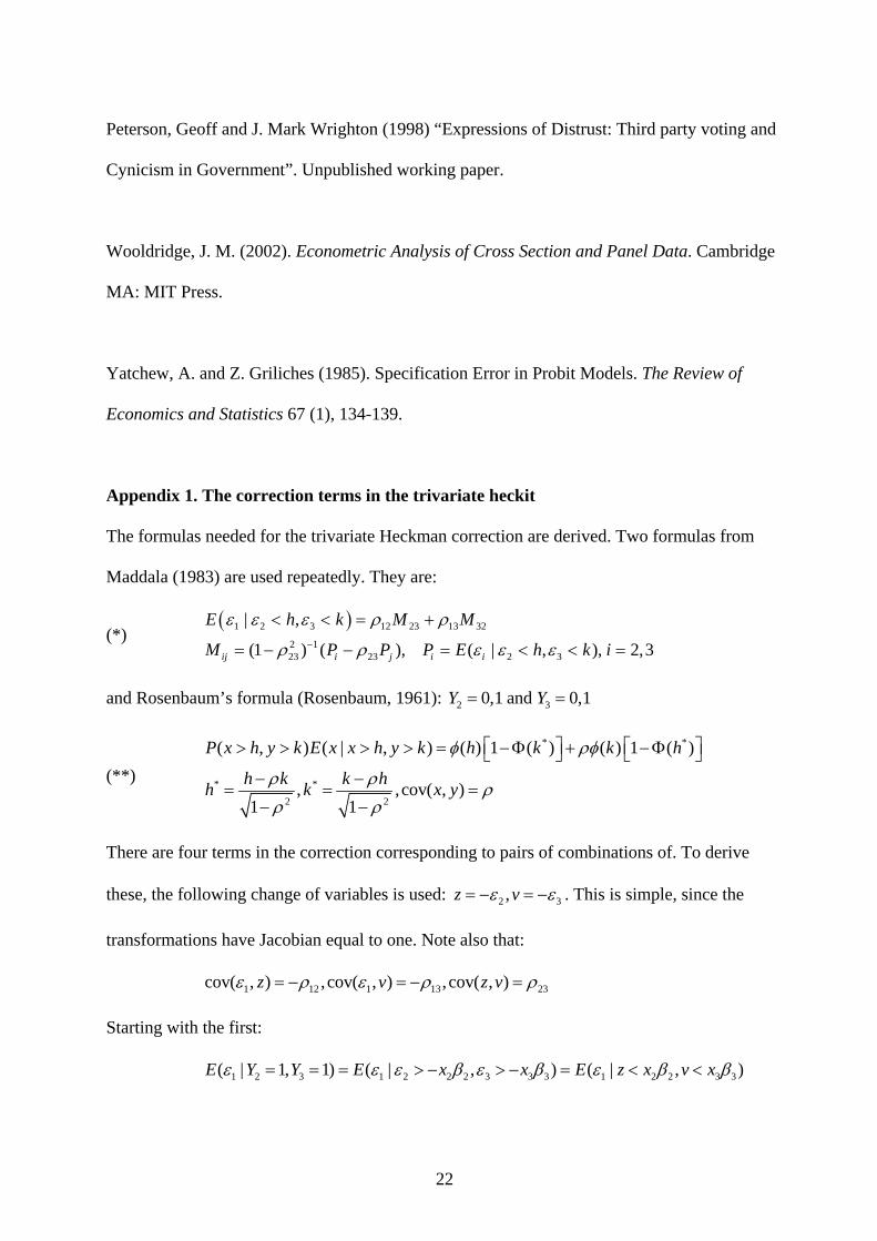
Appendix 1. The correction terms in the trivariate heckit

The formulas needed for the trivariate Heckman correction are derived. Two formulas from

Maddala (1983) are used repeatedly. They are:

(*) ( )1 2 3 12 23 13 32

2 123 23 2 3

| ,

(1 ) ( ), ( | , ), 2,3ij i j i i

E h k M M

M P P P E h k

ε ε ε ρ ρ

ρ ρ ε ε ε−

< < = +

= − − = < < =i

and Rosenbaum’s formula (Rosenbaum, 1961): 2 30,1 and 0,1Y Y= =

(**)

* *

* *

2 2

( , ) ( | , ) ( ) 1 ( ) ( ) 1 ( )

, , cov( , )1 1

P x h y k E x x h y k h k k h

h k k hh k x y

φ ρφ

ρ ρ ρρ ρ

⎡ ⎤ ⎡> > > > = − Φ + − Φ ⎤⎣ ⎦ ⎣− −

= = =− −

⎦

3

There are four terms in the correction corresponding to pairs of combinations of. To derive

these, the following change of variables is used: 2 ,z vε ε= − = − . This is simple, since the

transformations have Jacobian equal to one. Note also that:

1 12 1 13 23cov( , ) ,cov( , ) ,cov( , )z v z vε ρ ε ρ= − = − = ρ

Starting with the first:

1 2 3 1 2 2 2 3 3 3 1 2 2 3 3( | 1, 1) ( | , ) ( | , )E Y Y E x x E z x v xε ε ε β ε β ε β β= = = > − > − = < <

22

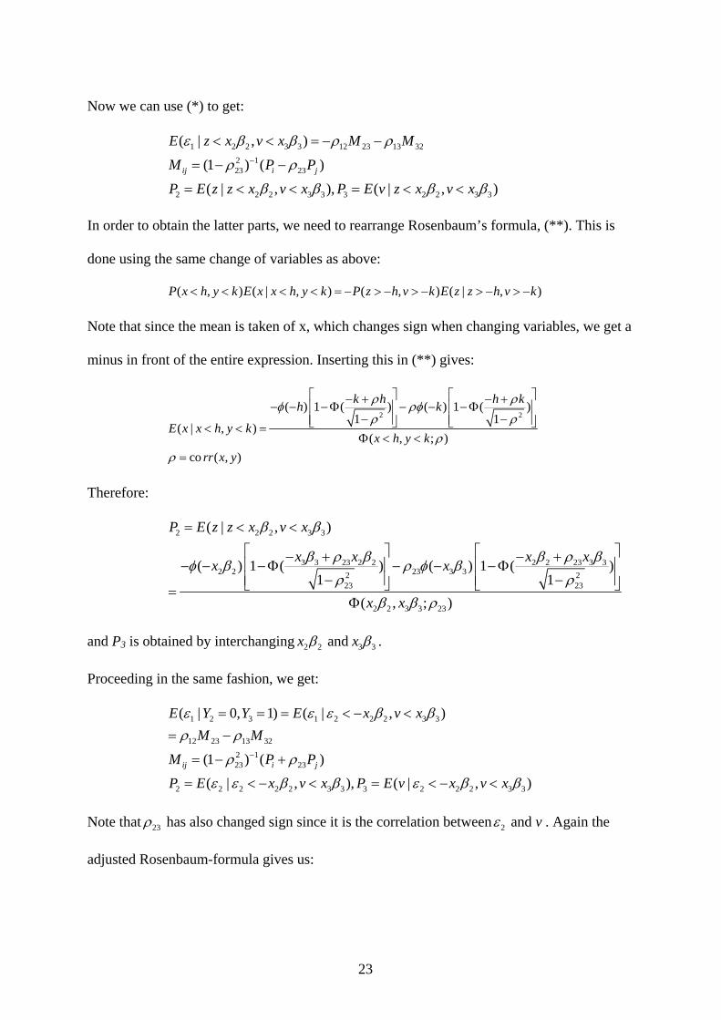
Now we can use (*) to get:

1 2 2 3 3 12 23 13 32

2 123 23

2 2 2 3 3 3 2 2

( | , )

(1 ) ( )

( | , ), ( | , )ij i j

E z x v x M M

M P P

P E z z x v x P E v z x v x

ε β β ρ ρ

ρ ρ

3 3β β β

−

< < = − −

= − −

= < < = < < β

In order to obtain the latter parts, we need to rearrange Rosenbaum’s formula, (**). This is

done using the same change of variables as above:

( , ) ( | , ) ( , ) ( | , )P x h y k E x x h y k P z h v k E z z h v k< < < < = − > − > − > − > −

Note that since the mean is taken of x, which changes sign when changing variables, we get a

minus in front of the entire expression. Inserting this in (**) gives:

2 2( ) 1 ( ) ( ) 1 ( )

1 1( | , )

( , ; )co ( , )

k h h kh k

E x x h y kx h y k

rr x y

ρ ρφ ρφρ ρ

ρρ

⎡ ⎤ ⎡− + − +− − − Φ − − − Φ⎤

⎢ ⎥ ⎢− −

⎥⎢ ⎥ ⎢ ⎥⎣ ⎦ ⎣< < =

Φ < <=

⎦

Therefore:

2 2 2 3 3

3 3 23 2 2 2 2 23 3 32 2 23 3 32 2

23 23

2 2 3 3 23

( | , )

( ) 1 ( ) ( ) 1 (1 1

( , ; )

P E z z x v x

x x x xx x

x x

)

β β

β ρ β β ρ βφ β ρ φ βρ ρ

β β ρ

= < <

⎡ ⎤ ⎡ ⎤− + − +⎢ ⎥ ⎢ ⎥− − − Φ − − − Φ⎢ ⎥ ⎢ ⎥− −⎣ ⎦ ⎣ ⎦=

Φ

and P3 is obtained by interchanging 2 2 3 3 and x xβ β .

Proceeding in the same fashion, we get:

1 2 3 1 2 2 2 3 3

12 23 13 32

2 123 23

2 2 2 2 2 3 3 3 2 2 2 3

( | 0, 1) ( | , )

(1 ) ( )

( | , ), ( | , )ij i j

E Y Y E x v xM M

M P P

P E x v x P E v x v x 3

ε ε ε β βρ ρ

ρ ρ

ε ε β β ε β β

−

= = = < − <= −

= − +

= < − < = < − <

Note that 23ρ has also changed sign since it is the correlation between 2 and vε . Again the

adjusted Rosenbaum-formula gives us:

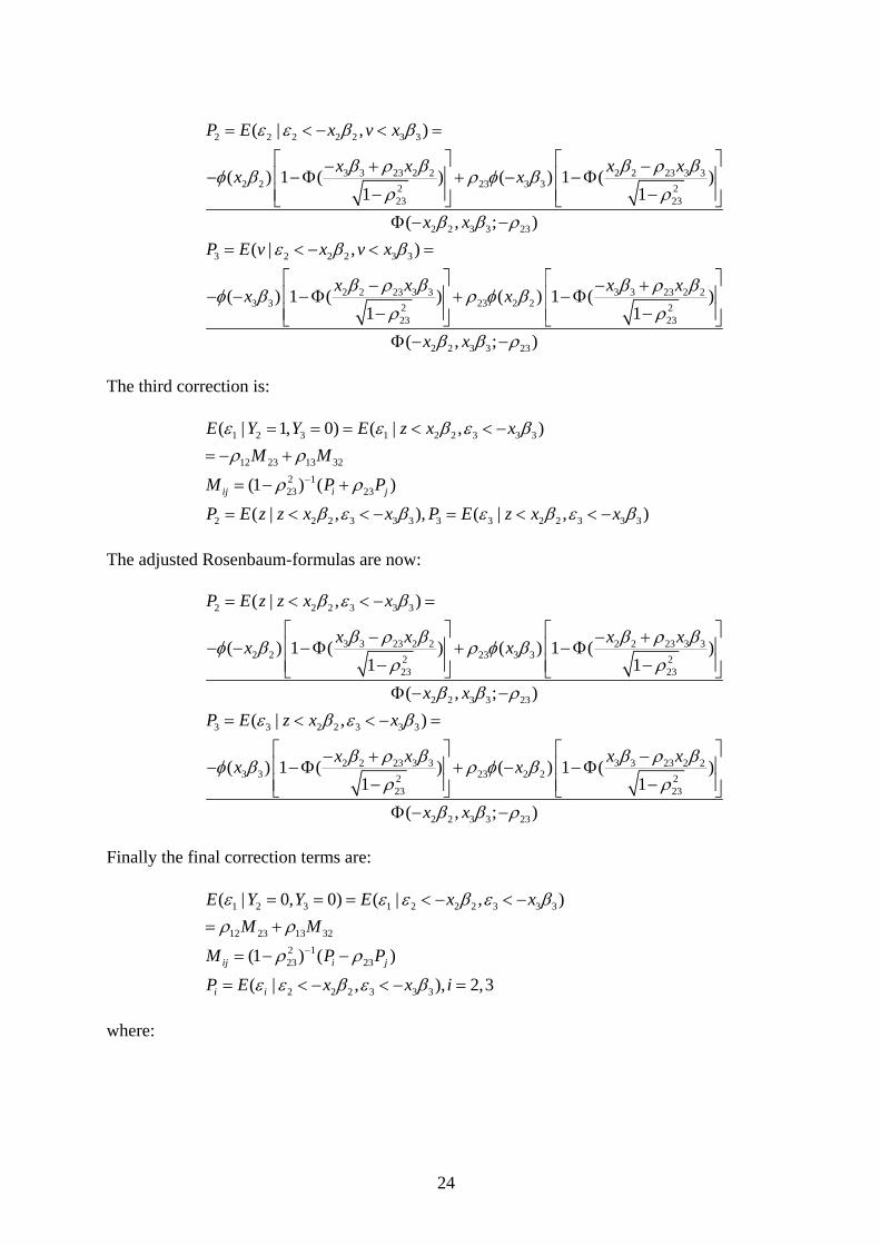
23

2 2 2 2 2 3 3

3 3 23 2 2 2 2 23 3 32 2 23 3 32 2

23 23

2 2 3 3 23

3 2 2 2 3 3

2 2 23 3 33 3 23 2 22

23

( | , )

( ) 1 ( ) ( ) 1 ( )1 1

( , ; )( | , )

( ) 1 ( ) (1

P E x v x

x x x xx x

x xP E v x v x

x xx x

ε ε β β

β ρ β β ρ βφ β ρ φ βρ ρ

β β ρε β β

β ρ βφ β ρ φ βρ

= < − < =

⎡ ⎤ ⎡− + −⎢ ⎥ ⎢− − Φ + − − Φ⎢ ⎥ ⎢− −⎣ ⎦ ⎣

Φ − −= < − < =

⎡ ⎤−⎢ ⎥− − − Φ +⎢ ⎥−⎣ ⎦

⎤⎥⎥⎦

3 3 23 2 2223

2 2 3 3 23

) 1 ( )1

( , ; )

x x

x x

β ρ βρ

β β ρ

⎡ ⎤− +⎢ ⎥− Φ⎢ ⎥−⎣ ⎦

Φ − −

The third correction is:

1 2 3 1 2 2 3 3 3

12 23 13 322 123 23

2 2 2 3 3 3 3 3 2 2 3

( | 1, 0) ( | , )

(1 ) ( )

( | , ), ( | , )ij i j

E Y Y E z x xM M

M P P

P E z z x x P E z x x3 3

ε ε β ε βρ ρ

ρ ρ

β ε β ε β ε β

−

= = = < < −= − +

= − +

= < < − = < < −

The adjusted Rosenbaum-formulas are now:

2 2 2 3 3 3

3 3 23 2 2 2 2 23 3 32 2 23 3 32 2

23 23

2 2 3 3 23

3 3 2 2 3 3 3

2 2 23 3 33 3 23 22

23

( | , )

( ) 1 ( ) ( ) 1 (1 1

( , ; )( | , )

( ) 1 ( ) (1

P E z z x x

x x x xx x

x xP E z x x

x xx x

)

β ε β

β ρ β β ρ βφ β ρ φ βρ ρ

β β ρε β ε β

β ρ βφ β ρ φ βρ

= < < − =

⎡ ⎤ ⎡− −⎢ ⎥ ⎢− − − Φ + − Φ⎢ ⎥ ⎢− −⎣ ⎦ ⎣

Φ − −

= < < − =

⎡ ⎤− +⎢ ⎥− − Φ + −⎢ ⎥−⎣ ⎦

⎤+⎥⎥⎦

3 3 23 2 22 2

23

2 2 3 3 23

) 1 ( )1

( , ; )

x x

x x

β ρ βρ

β β ρ

⎡ ⎤−⎢ ⎥− Φ⎢ ⎥−⎣ ⎦

Φ − −

Finally the final correction terms are:

1 2 3 1 2 2 2 3 3 3

12 23 13 322 123 23

2 2 2 3 3 3

( | 0, 0) ( | , )

(1 ) ( )

( | , ), 2,3ij i j

i i

E Y Y E x xM M

M P P

P E x x i

ε ε ε β ε βρ ρ

ρ ρ

ε ε β ε β

−

= = = < − < −= +

= − −

= < − < − =

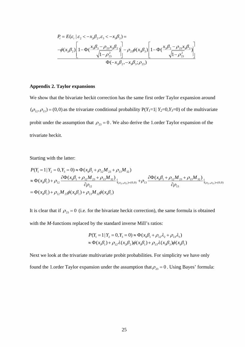
where:

24

2 2 2 3 3 3

3 3 23 2 2 2 2 23 3 32 2 23 3 32 2

23 23

2 2 3 3 23

( | , )

( ) 1 ( ) ( ) 1 ( )1 1

( , ; )

i iP E x x

x x x xx x

x x

ε ε β ε β

β ρ β β ρ βφ β ρ φ βρ ρ

β β ρ

= < − < − =

⎡ ⎤ ⎡ ⎤− −⎢ ⎥ ⎢ ⎥− − Φ − − Φ⎢ ⎥ ⎢ ⎥− −⎣ ⎦ ⎣ ⎦

Φ − −

Appendix 2. Taylor expansions

We show that the bivariate heckit correction has the same first order Taylor expansion around

12 13( , ) (0,0)ρ ρ = as the trivariate conditional probability P(Y1=1| Y2=0,Y3=0) of the multivariate

probit under the assumption that 23 0ρ = . We also derive the 1.order Taylor expansion of the

trivariate heckit.

Starting with the latter:

12 13 12 13

1 2 3 1 1 12 23 13 32

1 1 12 23 13 32 1 1 12 23 13 321 1 12 ( , ) (0,0) 13 ( , ) (0,0)

12 13

1 1 12 23 1 1 13 32 1 1

( 1| 0, 0) ( )( ) ( )( ) | |

( ) ( ) ( )

P Y Y Y x M Mx M M x M Mx

x M x M x

ρ ρ ρ ρ

β ρ ρβ ρ ρ β ρ ρβ ρ ρ

ρ ρβ ρ φ β ρ φ β

= =

= = = ≈ Φ + +∂Φ + + ∂Φ + +

≈ Φ + +∂ ∂

= Φ + +

It is clear that if 23 0ρ = (i.e. for the bivariate heckit correction), the same formula is obtained

with the M-functions replaced by the standard inverse Mill’s ratios:

1 2 3 1 1 12 2 13 3

1 1 12 2 2 1 1 13 3 3 1 1

( 1| 0, 0) ( )( ) ( ) ( ) ( ) ( )

P Y Y Y xx x x x x

β ρ λ ρ λβ ρ λ β φ β ρ λ β φ β

= = = ≈ Φ + +≈ Φ + +

Next we look at the trivariate multivariate probit probabilities. For simplicity we have only

found the 1.order Taylor expansion under the assumption that 23 0ρ = . Using Bayes’ formula:

25

1 2 3 2 3 1 1 2 1 3 1 1

1 2 1 3 1

1 2 3 1 2 1 3 1 2 3

( , , ) ( , | ) ( ) ( | ) ( | ) ( )( , ) ( , ) / ( )

. .( 1| 0, 0) ( 1, 0) ( 0, 0) /( ( 1) ( 0) ( 0

P Y Y Y P Y Y Y P Y P Y Y P Y Y P YP Y Y P Y Y P Y

i eP Y Y Y P Y Y P Y Y P Y P Y P Y

= ==

= = = = = = = = = = = ))

With the latent variable structure we can write these probabilities in the usual way with the

normal cdf evaluated at appropriate indices, which we for simplicity denotes by a’s here. The

Taylor-expansion of this is:

12 13

12

1 2 3 1 2 1 3 1 2 3

1 21 2 1 3 1 2 3 12 1 3 1 2 3 ( , ) (0,

12

1 313 2 3 1 2 3 (

13

( 1| 0, 0) ( , ) ( , ) /( ( ) ( ) ( ))( , )( ) ( ) ( ) ( ) /( ( ) ( ) ( )) [ ( , ) /( ( ) ( ) ( ))]

( , )[ ( , ) /( ( ) ( ) ( ))]

P Y Y Y a a a a a a aa aa a a a a a a a a a a a

a a a a a a a

ρ ρ

ρ

ρρ

ρρ

=

= = = = Φ Φ Φ Φ Φ ≈∂Φ

Φ Φ Φ Φ Φ Φ Φ + Φ Φ Φ Φ∂

∂Φ+ Φ Φ Φ Φ

∂ 13, ) (0,0)ρ =

0)

Noting that the derivative of the bivariate distribution function with respect to the correlation is

just the bivariate density, we get:

1 31 21 2 3 1 12 13

2 1

1 12 1 2 13 3 1

( ) ( )( ) ( )( 1| 0, 0) ( )( ) ( )

( ) ( ) ( ) ( ) ( )

a aa aP Y Y Y aa a

a a a a a

φ φφ φρ ρ

ρ φ λ ρ φ λ

= = = ≈ Φ + +Φ Φ

= Φ + +

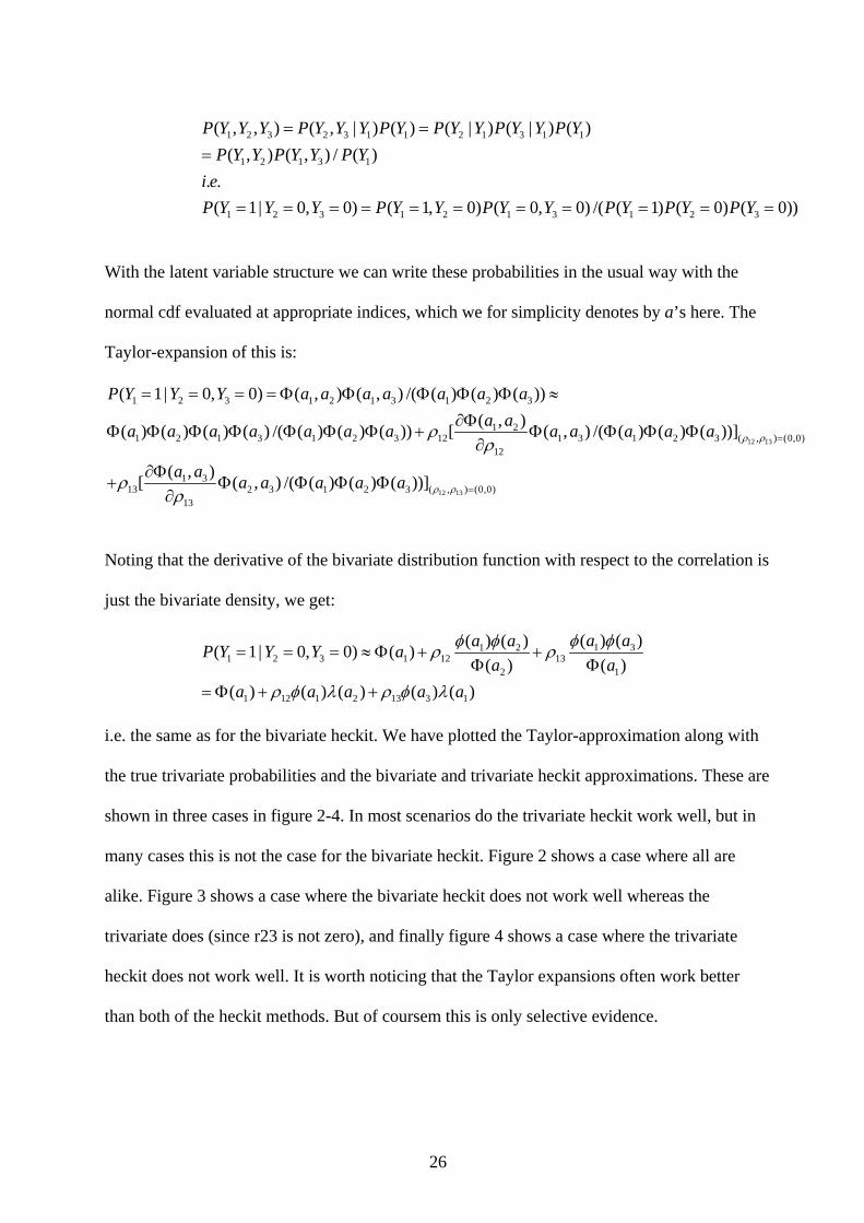
i.e. the same as for the bivariate heckit. We have plotted the Taylor-approximation along with

the true trivariate probabilities and the bivariate and trivariate heckit approximations. These are

shown in three cases in figure 2-4. In most scenarios do the trivariate heckit work well, but in

many cases this is not the case for the bivariate heckit. Figure 2 shows a case where all are

alike. Figure 3 shows a case where the bivariate heckit does not work well whereas the

trivariate does (since r23 is not zero), and finally figure 4 shows a case where the trivariate

heckit does not work well. It is worth noticing that the Taylor expansions often work better

than both of the heckit methods. But of coursem this is only selective evidence.

26

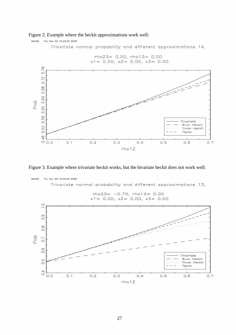
Figure 2. Example where the heckit approximations work well:

Figure 3. Example where trivariate heckit works, but the bivariate heckit does not work well:

27

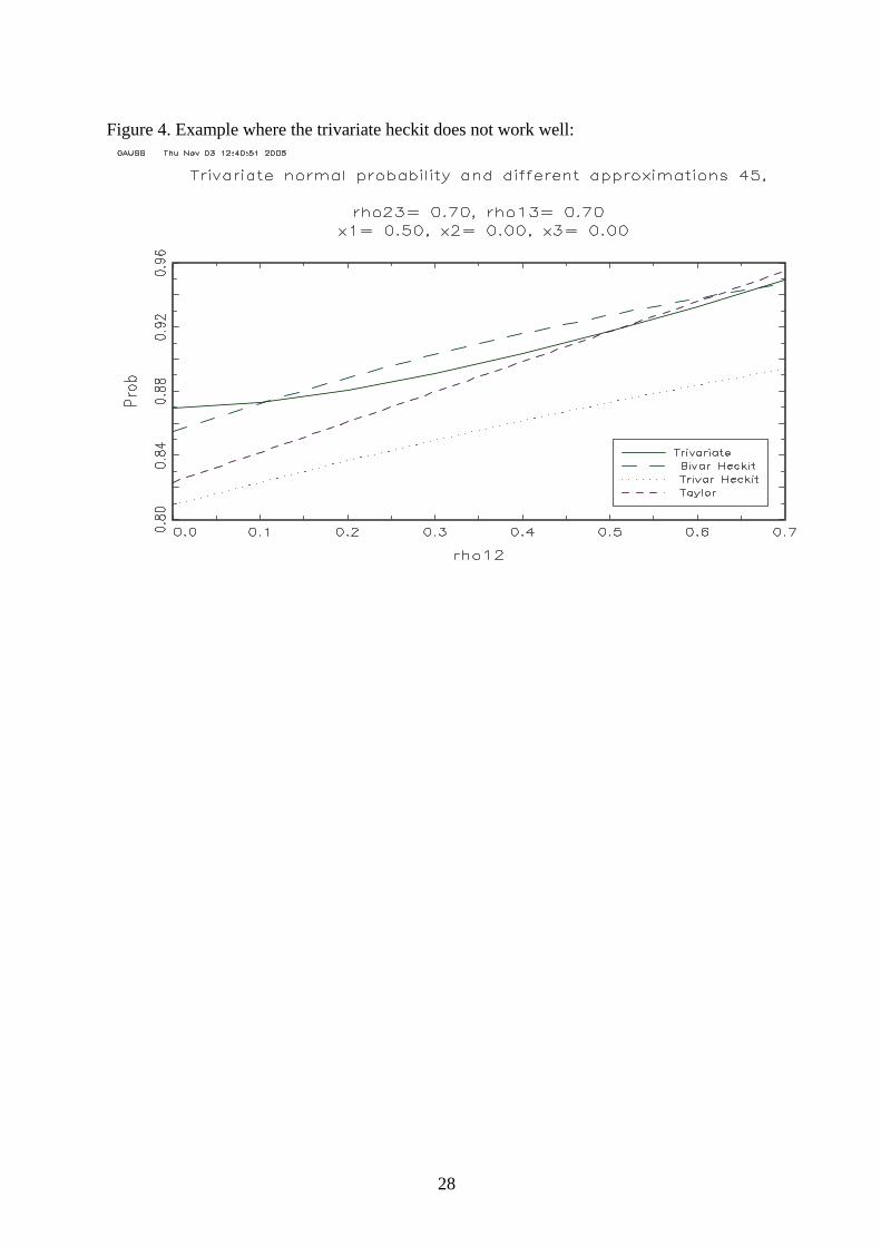
Figure 4. Example where the trivariate heckit does not work well:

28