Embed Size (px)
Citation preview
Detection of Electromagnetic Detection of Electromagnetic RadiationRadiation
Phil Mauskopf, University of Phil Mauskopf, University of RomeRome
12/14 January, 200412/14 January, 2004
The Ultimate Radiation DetectorsGoals -
Particle point of view:Measure for each photon 1) Arrival time 2) Energy and direction (momentum) 3) Polarization
Wave point of view:Measure the E (and/or B) field: 1) Amplitude and phase 2) Frequency 3) Polarization
The Ultimate Limit:
Quantum fluctuations in the signalParticle point of view:- Can’t know both the arrival time and the photon energy simultaneouslyWave point of view:- Can’t know both the amplitude and phase simultaneously
So: How close are we?
Depends on overall instrument design...
How to design an instrument:
Define requirements - like an engineer:
1. Angular resolution required?2. Sensitivity required - intensity of source?3. Dynamic range - minimum vs. maximum signal?4. Speed of response required - fastest change in signal?5. Frequency bandwidth of source?6. Frequency resolution required?7. Polarisation discrimination required?
1. Angular resolution required optics design
Fundamentally limited by diffraction
2. Sensitivity required collecting area, number of detectors, detector and optics configuration
Fundamentally limited by photon noise from source
3. Dynamic range detector and readout type
4. Speed of response required detector and readout type
5. Frequency bandwidth of source filtering system
6. Frequency resolution required filtering and detectors
7. Polarisation discrimination required
Design tools:
Optics: ZeMAX, CODEV, GRASP, etc.- Ray tracing- Fraunhofer diffraction- Physical optics calculationsOnly limited by complexity of optics and computing power
Complex structures - I.e. waveguides, transmission lines:HFSS, ADS, SONNET, etc.- 2-D and 3-D solutions to Maxwell’s equations- Full calculation of electric and magnetic fieldsOnly limited by complexity of structures and computing power
Need to know basics in order to make reasonably simple designNormally courses on electromagnetics discuss methods ofsolving Maxwell’s equations with a variety of boundary conditionsOnly necessary today if you don’t own a computer...
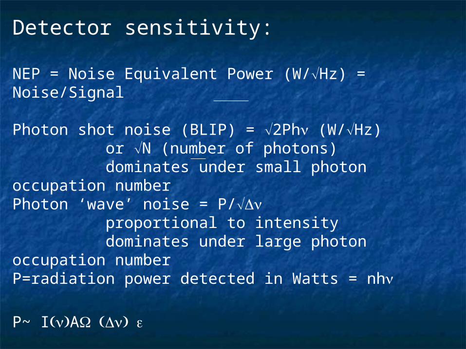
Detector sensitivity:
NEP = Noise Equivalent Power (W/Hz) = Noise/Signal
Photon shot noise (BLIP) = 2Ph (W/Hz)or N (number of photons)dominates under small photon occupation number
Photon ‘wave’ noise = P/proportional to intensitydominates under large photon occupation number
P=radiation power detected in Watts = nh
P~ IA
so if we know the source intensity, throughput and resolution we can calculate the sensitivity limit (and necessary detector sensitivity)
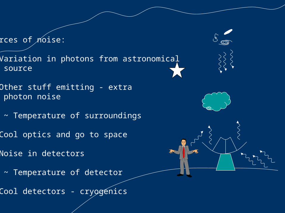
Sources of noise:
1) Variation in photons from astronomical source
2) Other stuff emitting - extra photon noise
~ Temperature of surroundings
=> Cool optics and go to space
3) Noise in detectors
~ Temperature of detector
=> Cool detectors - cryogenics
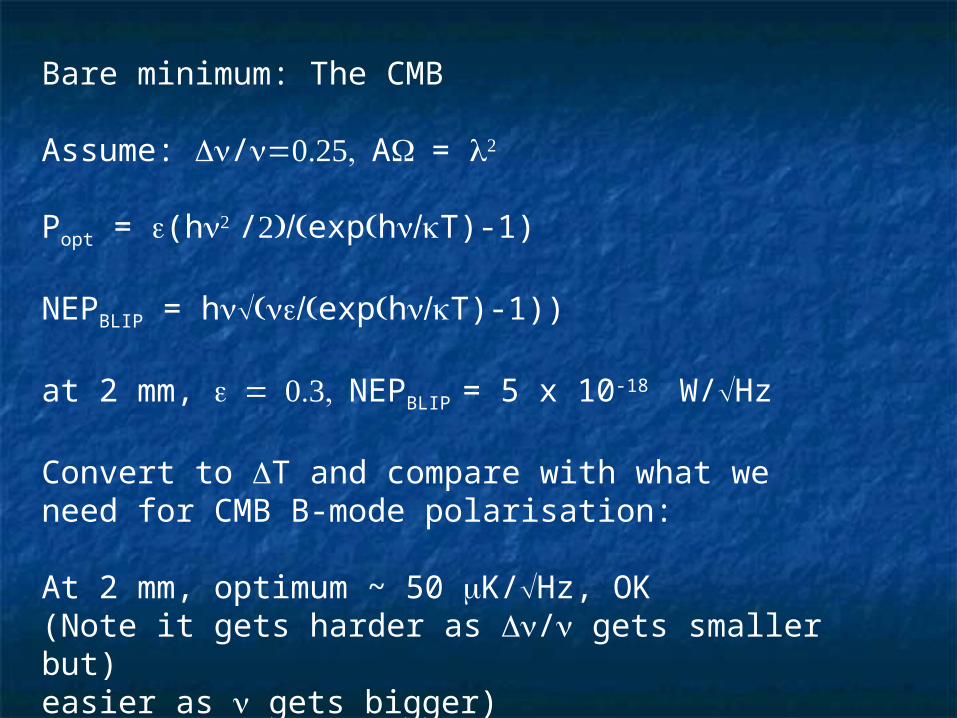
Bare minimum: The CMB
Assume: /A=
Popt = (h/exphT)-1)
NEPBLIP = hexphT)-1))
at 2 mm, NEPBLIP = 5 x 10-18 W/Hz
Convert to T and compare with what weneed for CMB B-mode polarisation:
At 2 mm, optimum ~ 50 K/Hz, OK(Note it gets harder as / gets smaller but)easier as gets bigger)
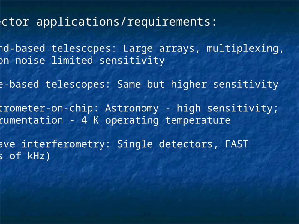
Detector applications/requirements:
Ground-based telescopes: Large arrays, multiplexing,photon noise limited sensitivity
Space-based telescopes: Same but higher sensitivity
Spectrometer-on-chip: Astronomy - high sensitivity;instrumentation - 4 K operating temperature
mm-wave interferometry: Single detectors, FAST(tens of kHz)
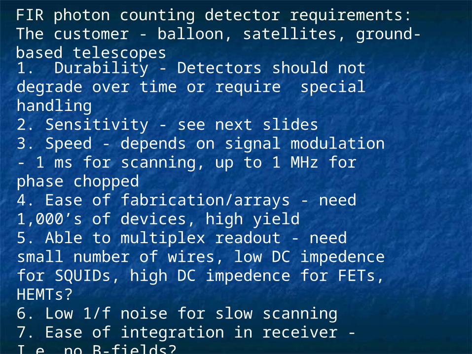
FIR photon counting detector requirements:The customer - balloon, satellites, ground-based telescopes
1. Durability - Detectors should not degrade over time or require special handling2. Sensitivity - see next slides3. Speed - depends on signal modulation - 1 ms for scanning, up to 1 MHz for phase chopped4. Ease of fabrication/arrays - need 1,000’s of devices, high yield5. Able to multiplex readout - need small number of wires, low DC impedence for SQUIDs, high DC impedence for FETs, HEMTs?6. Low 1/f noise for slow scanning7. Ease of integration in receiver - I.e. no B-fields?8. Ease of coupling power - 50 Ohm RF impedence or separate detector/thermometer and absorber
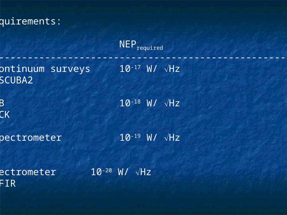
Sensitivity requirements:
Experiment NEPrequired
------------------------------------------------------------------------Ground-based continuum surveys 10-17 W/ Hze.g. BOLOCAM, SCUBA2
Space-based CMB 10-18 W/ Hze.g. post-PLANCK
Ground-based spectrometer 10-19 W/ Hze.g. z-spec
Space-based spectrometer 10-20 W/ Hze.g. SPECS, SAFIR
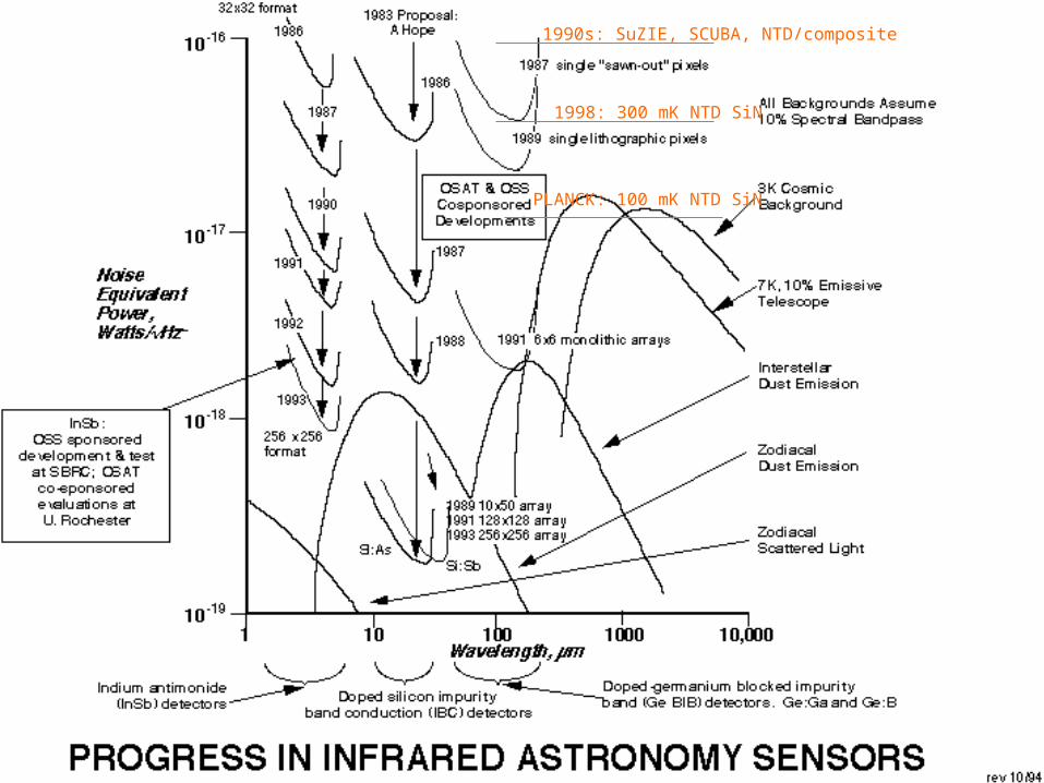
1990s: SuZIE, SCUBA, NTD/composite
1998: 300 mK NTD SiN
PLANCK: 100 mK NTD SiN
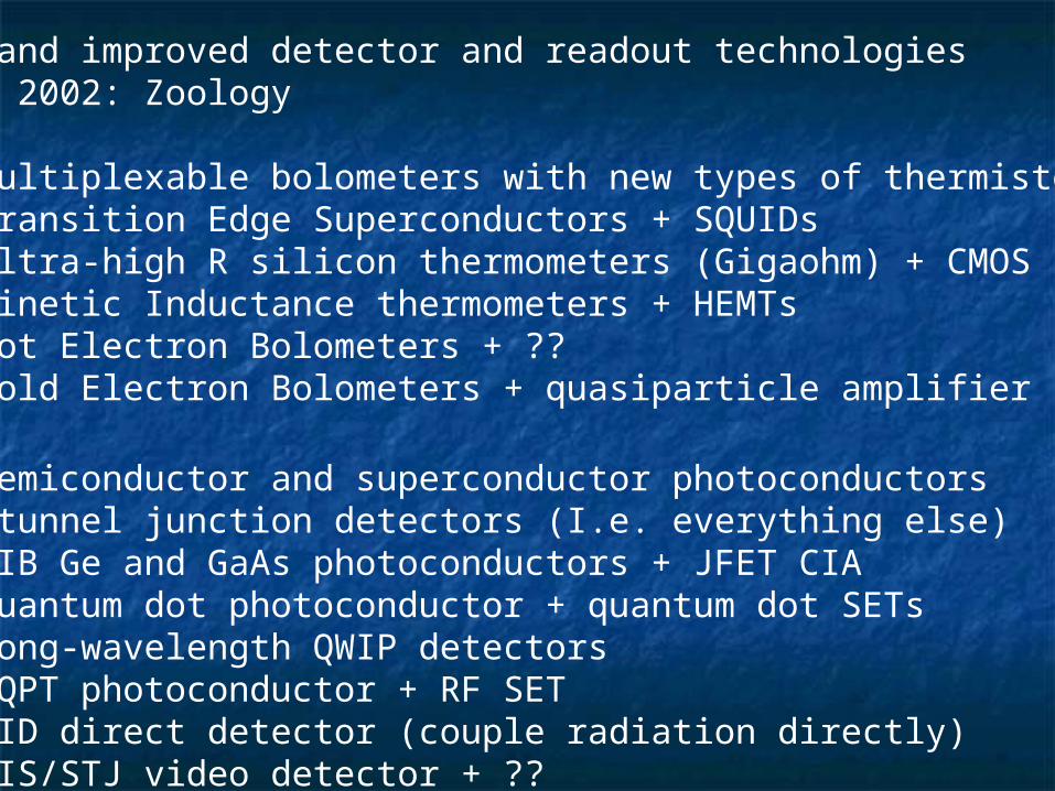
New and improved detector and readout technologiesc.f. 2002: Zoology
1. Multiplexable bolometers with new types of thermistors• Transition Edge Superconductors + SQUIDs• Ultra-high R silicon thermometers (Gigaohm) + CMOS• Kinetic Inductance thermometers + HEMTs• Hot Electron Bolometers + ??• Cold Electron Bolometers + quasiparticle amplifier
2. Semiconductor and superconductor photoconductorsand tunnel junction detectors (I.e. everything else)• BIB Ge and GaAs photoconductors + JFET CIA• Quantum dot photoconductor + quantum dot SETs• Long-wavelength QWIP detectors• SQPT photoconductor + RF SET• KID direct detector (couple radiation directly)• SIS/STJ video detector + ??
To understand how these detectors work and can beused in an instrument, we have to do some backgroundreview
Things that you always thought you understood untilyou had to teach them:
• Propagation of electromagnetic radiation• Transmission lines and waveguides• Geometrical, diffraction and physical optics• Scattering matrix for linear systems• Photon statistics and noise
Today: Lightning review of radiation, transmission lines
Friday: Lightning review of optics and scattering matrix
Monday: Photon statistics and noise + periodic structures and filters?
Tuesday?: Instrument configurations - spectrometers,interferometers, imagers
Wednesday: Detectors I
Friday: Detectors II + readouts
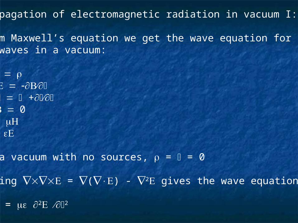
Propagation of electromagnetic radiation in vacuum I:
From Maxwell’s equation we get the wave equation forEM waves in a vacuum:
+0
In a vacuum with no sources, = = 0
Taking = () - 2 gives the wave equation
2 = 2 2
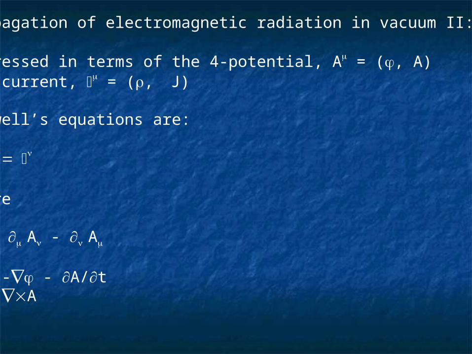
Propagation of electromagnetic radiation in vacuum II:
Expressed in terms of the 4-potential, A = (, A)and current, = (, J)
Maxwell’s equations are:
where
A - A
E = - - A/tB = A
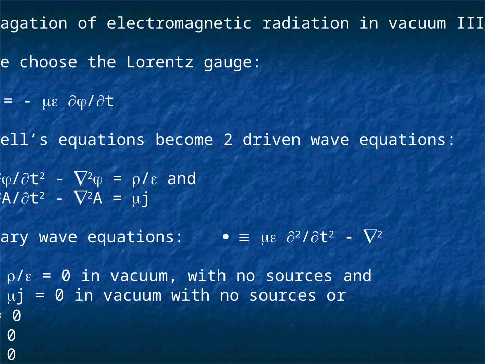
Propagation of electromagnetic radiation in vacuum III:
If we choose the Lorentz gauge:
A = - /t
Maxwell’s equations become 2 driven wave equations:
2/t2 - 2 = / and 2A/t2 - 2A = j
Summary wave equations: 2/t2 - 2
= / = 0 in vacuum, with no sources andA = j = 0 in vacuum with no sources orA = 0E = 0B = 0
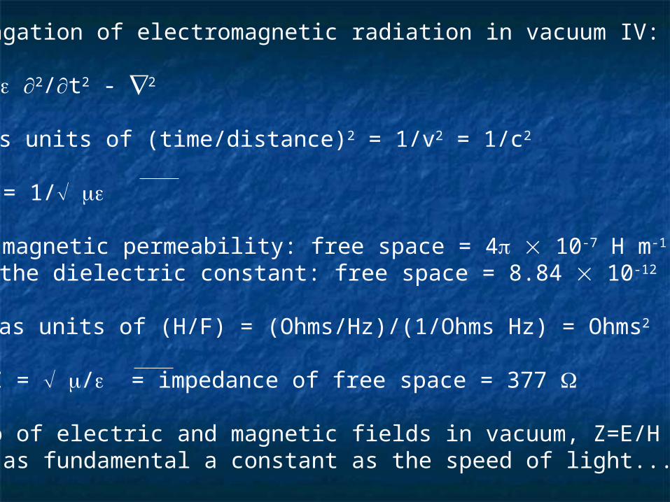
Propagation of electromagnetic radiation in vacuum IV:
2/t2 - 2
has units of (time/distance)2 = 1/v2 = 1/c2
or c = 1/
is magnetic permeability: free space = 4 10-7 H m-1
is the dielectric constant: free space = 8.84 10-12 F m-1
/ has units of (H/F) = (Ohms/Hz)/(1/Ohms Hz) = Ohms2
So, Z = / = impedance of free space = 377
Ratio of electric and magnetic fields in vacuum, Z=E/HJust as fundamental a constant as the speed of light...
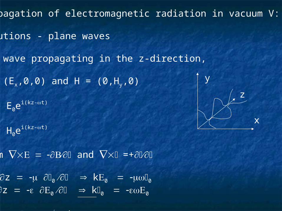
Propagation of electromagnetic radiation in vacuum V:
Solutions - plane waves
For wave propagating in the z-direction,
E = (Ex,0,0) and H = (0,Hy,0)
Ex = E0ei(kz-t)
Hy = H0ei(kz-t)
From and =+
0 z 0 k0 0 0 z 0 k0 0
and 0 0 /
x
y
z
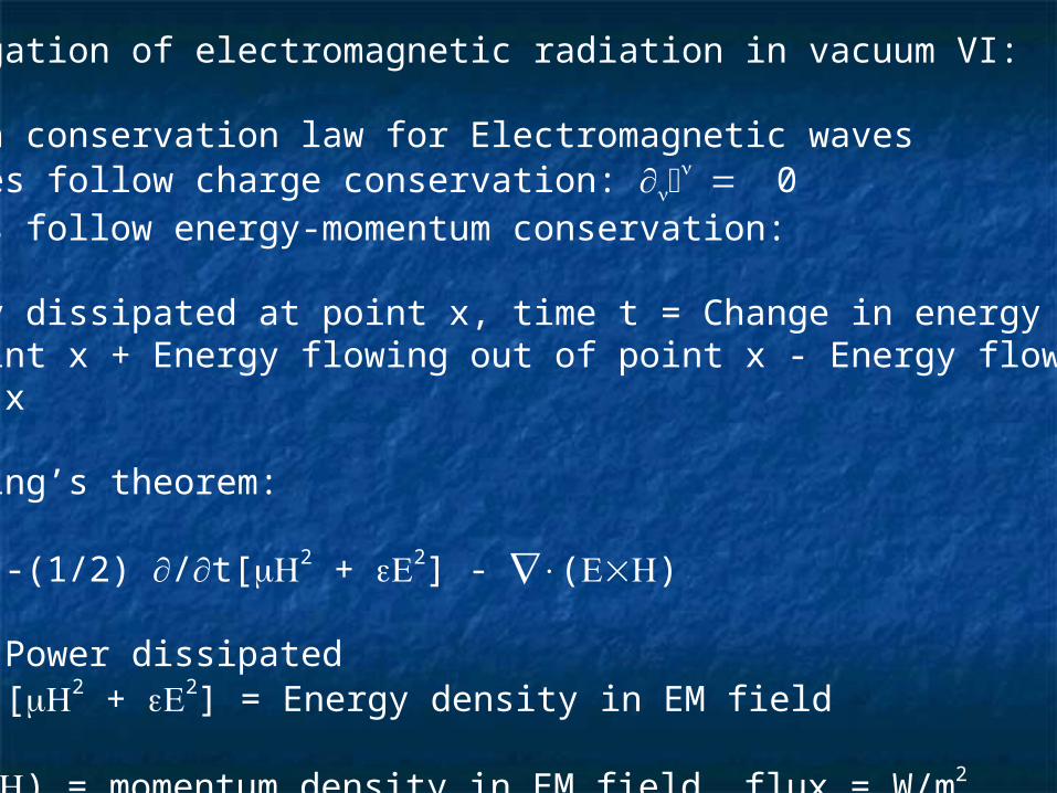
Propagation of electromagnetic radiation in vacuum VI:
Find a conservation law for Electromagnetic wavesSources follow charge conservation:
0Fields follow energy-momentum conservation:
Energy dissipated at point x, time t = Change in energy in fieldat point x + Energy flowing out of point x - Energy flowing intopoint x
Poynting’s theorem:
E·J = -(1/2) /t[2 + 2] - ()
E·J = Power dissipated(1/2) [2 + 2] = Energy density in EM field
() = momentum density in EM field, flux = W/m2
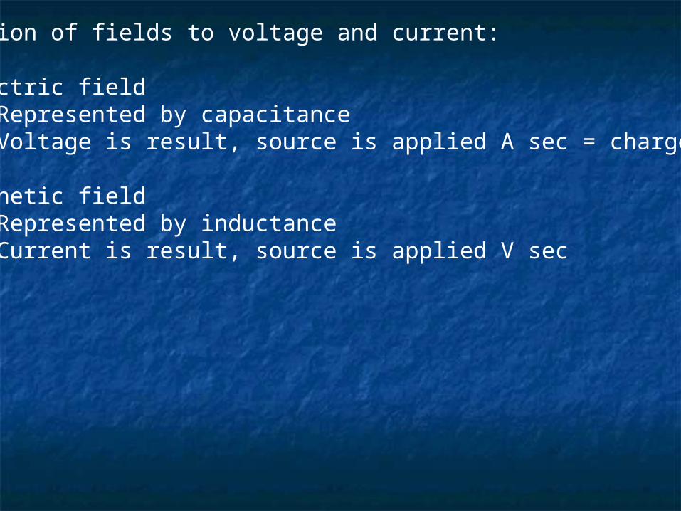
Relation of fields to voltage and current:
• Electric field - Represented by capacitance - Voltage is result, source is applied A sec = charge
• Magnetic field - Represented by inductance - Current is result, source is applied V sec
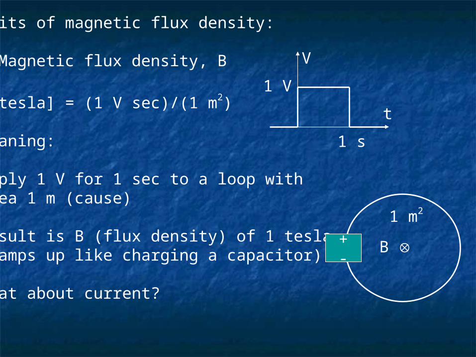
Units of magnetic flux density:
• Magnetic flux density, B
[tesla] = (1 V sec)/(1 m2)
Meaning:
Apply 1 V for 1 sec to a loop witharea 1 m (cause)
Result is B (flux density) of 1 tesla(ramps up like charging a capacitor)
What about current?
V
t
1 V
1 s
+-
1 m2
B
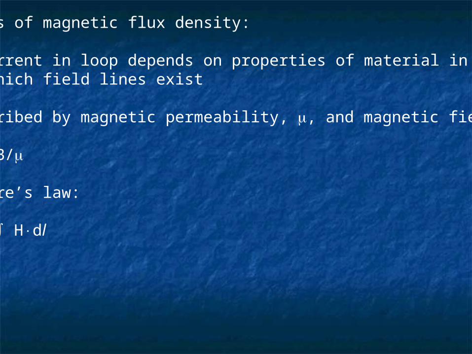
Units of magnetic flux density:
• Current in loop depends on properties of material in which field lines exist
Described by magnetic permeability, , and magnetic field, H
H = B/
Ampere’s law:
I = Hdl
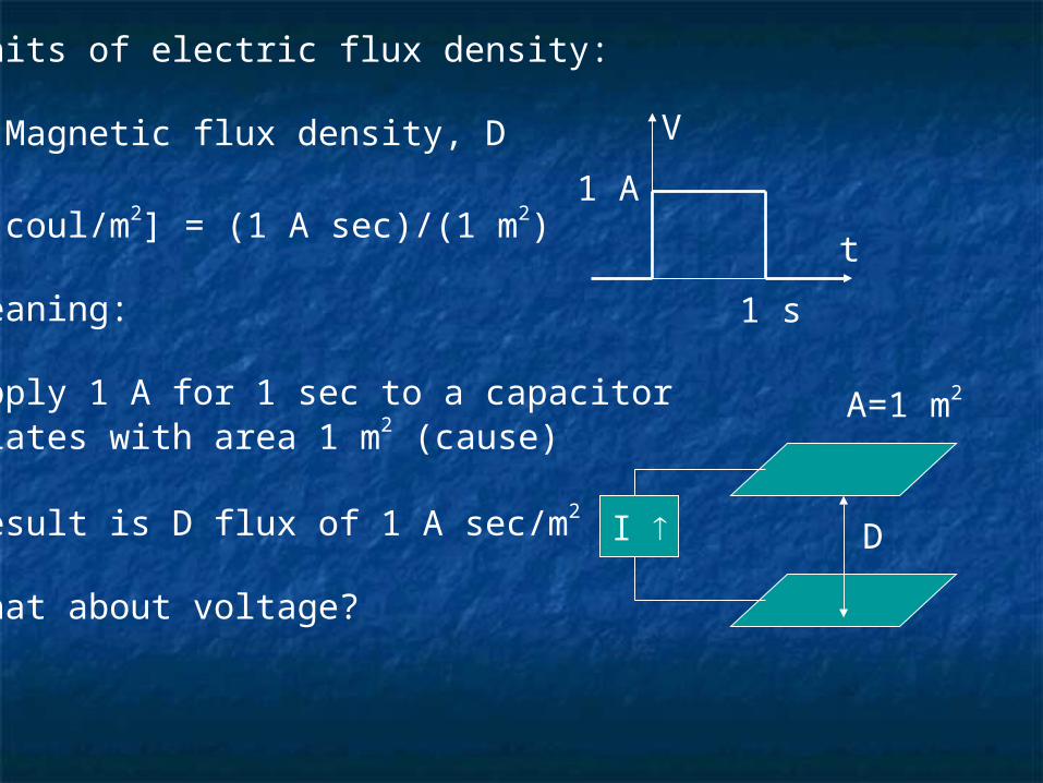
Units of electric flux density:
• Magnetic flux density, D
[coul/m2] = (1 A sec)/(1 m2)
Meaning:
Apply 1 A for 1 sec to a capacitorplates with area 1 m2 (cause)
Result is D flux of 1 A sec/m2
What about voltage?
V
t
1 A
1 s
I
A=1 m2
D
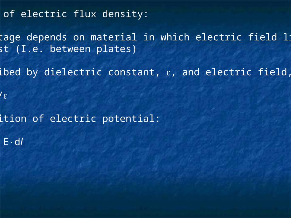
Units of electric flux density:
• Voltage depends on material in which electric field lines exist (I.e. between plates)
Described by dielectric constant, , and electric field, E
E = D/
Definition of electric potential:
V = Edl
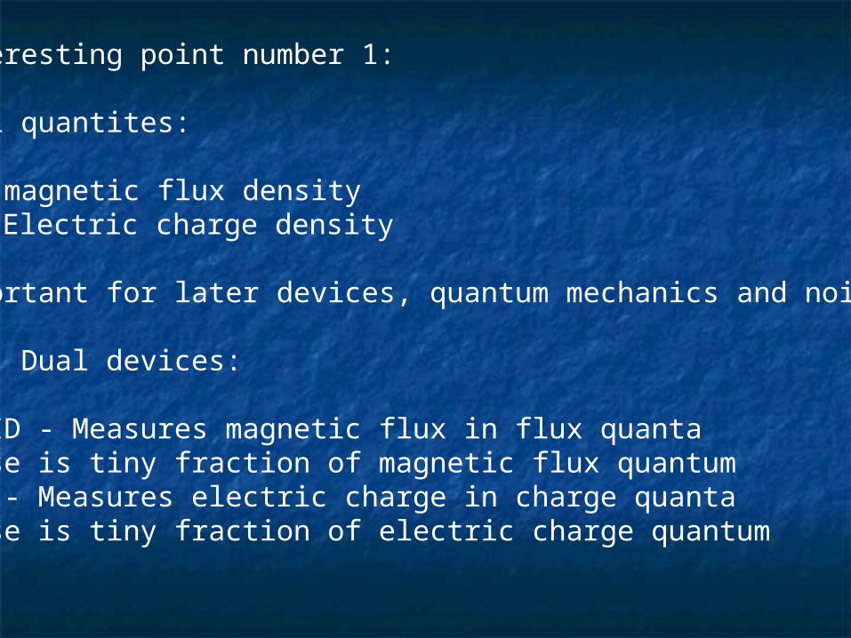
Interesting point number 1:
Dual quantites:
B - magnetic flux density - Electric charge density
Important for later devices, quantum mechanics and noise:
E.g. Dual devices:
SQUID - Measures magnetic flux in flux quantaNoise is tiny fraction of magnetic flux quantumSET - Measures electric charge in charge quantaNoise is tiny fraction of electric charge quantum
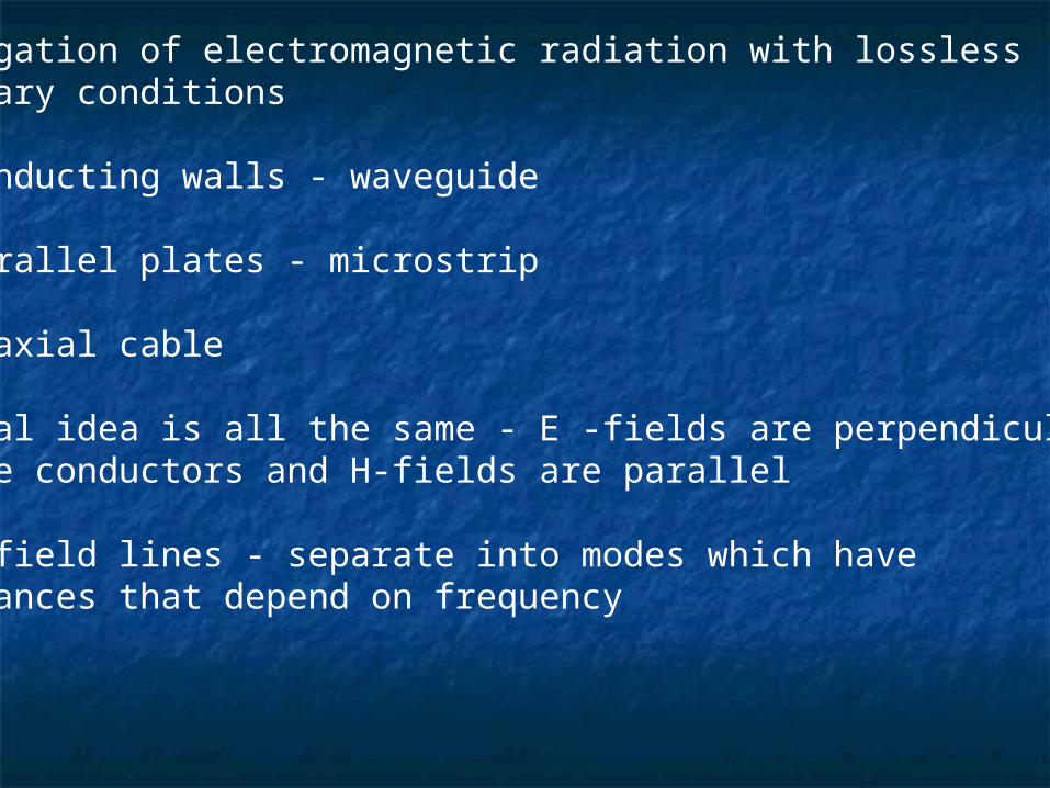
Propagation of electromagnetic radiation with losslessboundary conditions
1. Conducting walls - waveguide
2. Parallel plates - microstrip
3. Coaxial cable
General idea is all the same - E -fields are perpendicularto the conductors and H-fields are parallel
Draw field lines - separate into modes which haveimpedances that depend on frequency
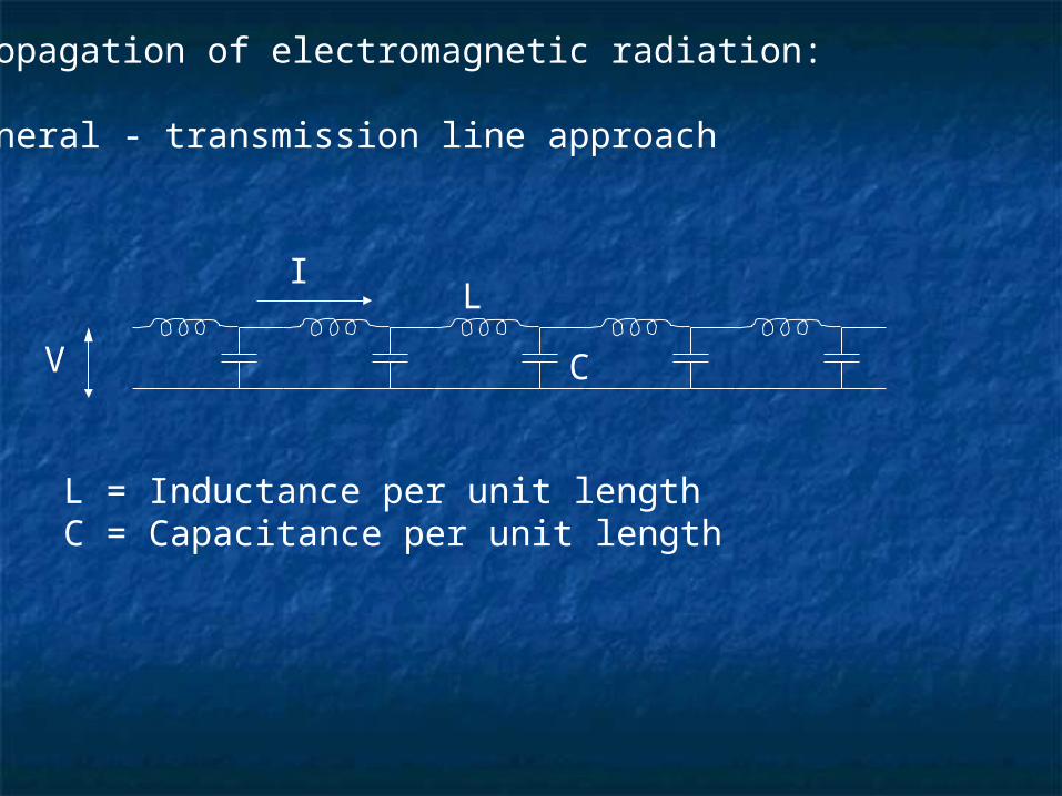
Propagation of electromagnetic radiation:
General - transmission line approach
V
IL
C
L = Inductance per unit lengthC = Capacitance per unit length
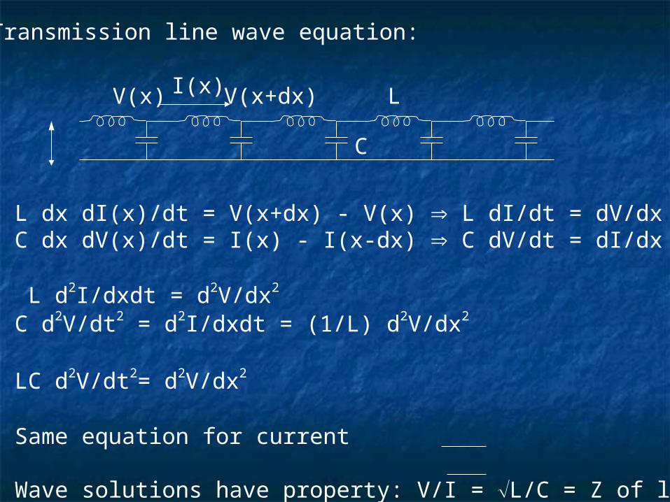
Transmission line wave equation:
V(x) I(x) L
C
L dx dI(x)/dt = V(x+dx) - V(x) L dI/dt = dV/dx C dx dV(x)/dt = I(x) - I(x-dx) C dV/dt = dI/dx
L d2I/dxdt = d2V/dx2
C d2V/dt2 = d2I/dxdt = (1/L) d2V/dx2
LC d2V/dt2= d2V/dx2
Same equation for current
Wave solutions have property: V/I = L/C = Z of line v2 = 1/LC = speed of prop.
V(x+dx)
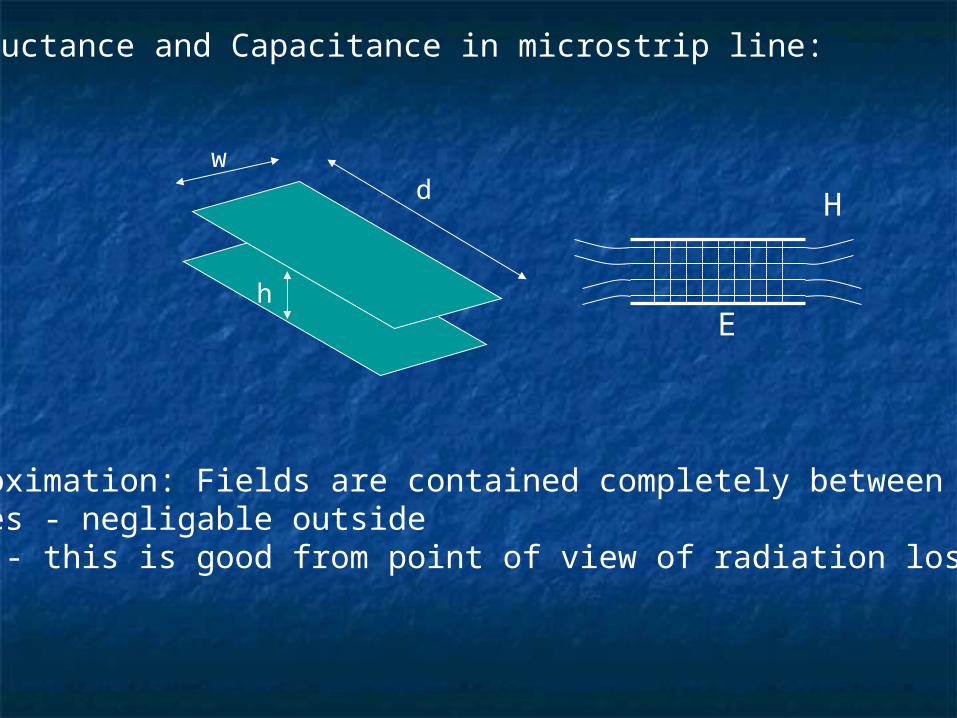
Inductance and Capacitance in microstrip line:
w
h
d H
E
Approximation: Fields are contained completely betweenplates - negligable outsideNote - this is good from point of view of radiation losses,etc.
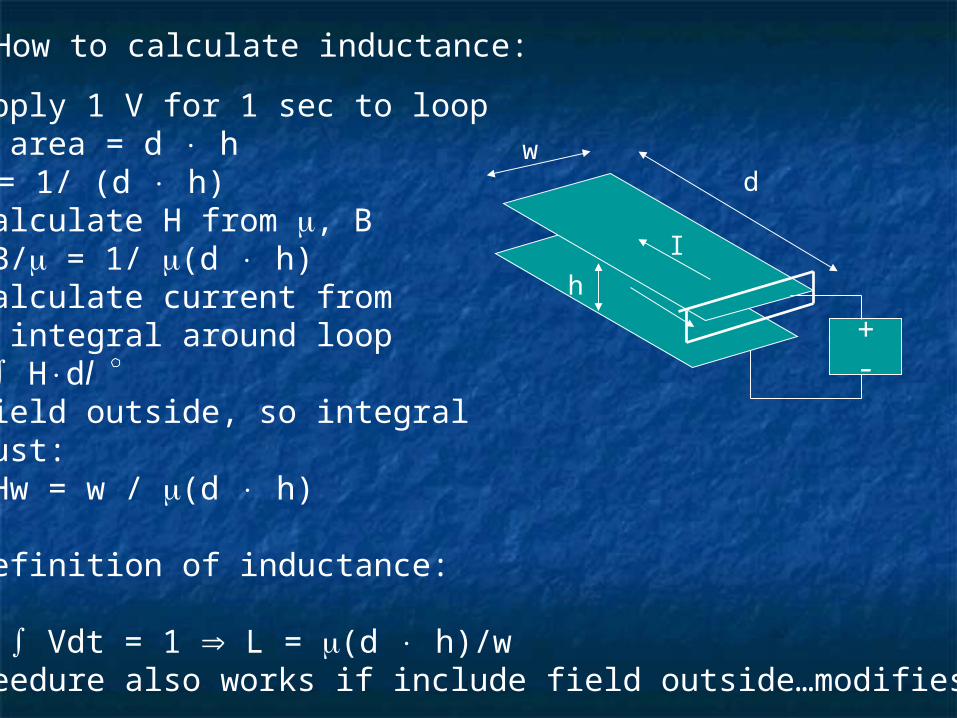
How to calculate inductance:
w
h
I
+-
1. Apply 1 V for 1 sec to loopwith area = d h B = 1/ (d h)2. Calculate H from , BH = B/ = 1/ (d h)3. Calculate current frompath integral around loopI = HdlNo field outside, so integralis just:I = Hw = w / (d h)
4. Definition of inductance:
LI = Vdt = 1 L = (d h)/wProceedure also works if include field outside…modifies L
d
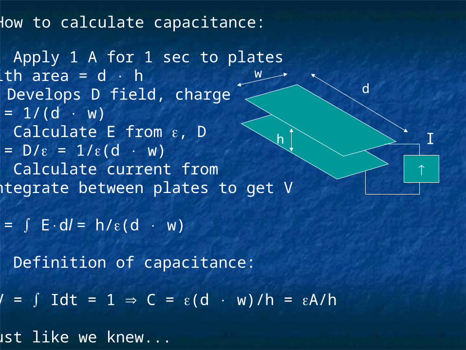
How to calculate capacitance:
w
h
1. Apply 1 A for 1 sec to plateswith area = d h Develops D field, chargeD = 1/(d w)2. Calculate E from , DE = D/ = 1/(d w)3. Calculate current fromIntegrate between plates to get V
V = Edl = h/(d w)
4. Definition of capacitance:
CV = Idt = 1 C = (d w)/h = A/h
Just like we knew...
d
I
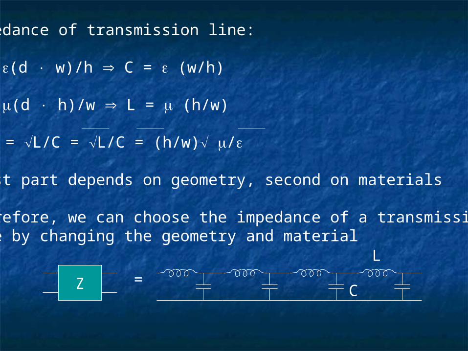
Impedance of transmission line:
C = (d w)/h C = (w/h)
L = (d h)/w L = (h/w)
Z = L/C = L/C = (h/w) /
First part depends on geometry, second on materials
Therefore, we can choose the impedance of a transmissionline by changing the geometry and material
Z =
L
C
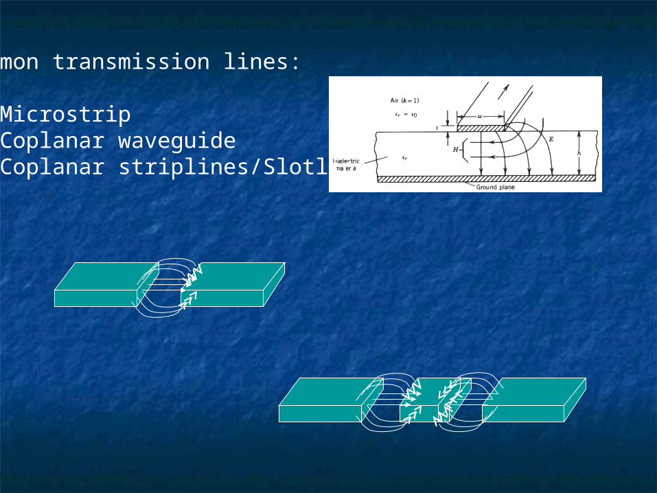
Common transmission lines:
1. Microstrip2. Coplanar waveguide3. Coplanar striplines/Slotline
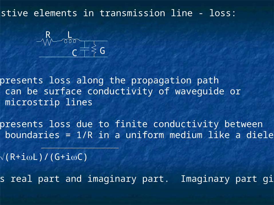
Resistive elements in transmission line - loss:
C
R
G
L
R represents loss along the propagation path can be surface conductivity of waveguide or microstrip lines
G represents loss due to finite conductivity between boundaries = 1/R in a uniform medium like a dielectric
Z = (R+iL)/(G+iC)
Z has real part and imaginary part. Imaginary part givesloss
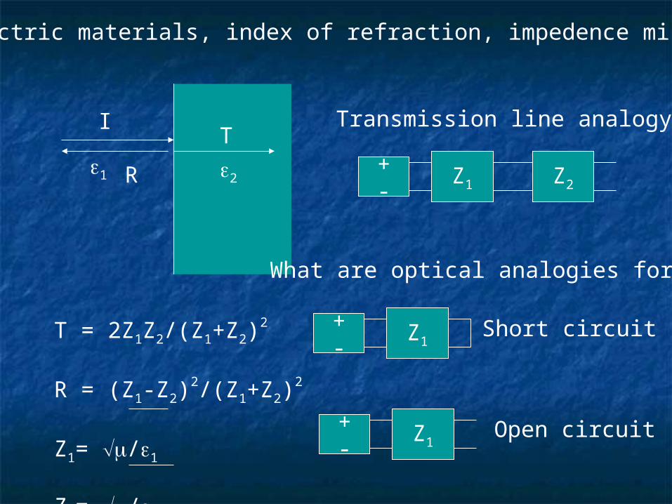
Dielectric materials, index of refraction, impedence mismatch:
1 2
IT
R
T = 2Z1Z2/(Z1+Z2)2
R = (Z1-Z2)2/(Z1+Z2)
2
Z1= /1
Z2= /2
Z1 Z2
Transmission line analogy
Z1
What are optical analogies for:
Short circuit
Z1Open circuit
+-
+-
+-
Circuit design in the GHz age:
Lumped elements vs. transmission line
Used to designing circuits with capacitors and inductorswith wire leads?
When the size of the component approaches the wavelengthof the EM signal propagating in the component, transmissionline analysis becomes important…
c.f. New computers with clock speeds of 100 GHz…1 THz?
Propagation of electromagnetic radiation in vacuum V:
Solutions - with boundary conditions
Parallel conducting platesEnclose in conducting walls - waveguideCoaxial cableMicro-strip lineCoplanar waveguideCoplanar striplinesSlotlineetc.
Given that the solution for the propagation of EM wavesis different for each of the above types of boundary conditions,how do we transform a giant plane wave coming from a distantsource into a wave travelling down a tiny transmission linewithout losing information? - Answer: optics