Detection of Stacked Filament Lensing Between SDSS

Mon. Not. R. Astron. Soc. 000, 000–000 (0000) Printed 1 February 2016 (MN LATEX style file v2.2)

Detection of Stacked Filament Lensing Between SDSSLuminous Red Galaxies

Joseph Clampitt1?, Hironao Miyatake2,3,4, Bhuvnesh Jain1, Masahiro Takada31Department of Physics and Astronomy, University of Pennsylvania, 209 S. 33rd St., Philadelphia, PA 19104, USA2Department of Astrophysical Sciences, Princeton University, Peyton Hall, Princeton NJ 08544, USA3Kavli Institute for the Physics and Mathematics of the Universe (Kavli IPMU, WPI), The University of Tokyo, Chiba 277-8583, Japan4Jet Propulsion Laboratory, California Institute of Technology, Pasadena, CA 91109

1 February 2016

ABSTRACTWe search for the lensing signal of massive filaments between 135,000 pairs of LuminousRed Galaxies (LRGs) from the Sloan Digital Sky Survey. We develop a new estimatorthat cleanly removes the much larger shear signal of the neighboring LRG halos,relying only on the assumption of spherical symmetry. We consider two models: a“thick” filament model constructed from ray-tracing simulations for ΛCDM model, anda “thin” filament model which models the filament by a string of halos along the lineconnecting the two LRGs. We show that the filament lensing signal is in nice agreementwith the thick simulation filament, while strongly disfavoring the thin model. Themagnitude of the lensing shear due to the filament is below 10−4. Employing thelikelihood ratio test, we find a 4.5σ significance for the detection of the filament lensingsignal, corresponding to a null hypothesis fluctuation probability of 3× 10−6. We alsocarried out several null tests to verify that the residual shear signal from neighboringLRGs and other shear systematics are minimized.

Key words: cosmology: observations – dark matter – large scale structure of Uni-verse; gravitational lensing: weak

1 INTRODUCTION

One of the most striking features of N -body simulations forΛCDM structure formation scenario is the network of fila-ments into which dark matter particles arrange themselves.Some attempts to quantify this network have been made(Sousbie 2011; Cautun et al. 2014). Other work has at-tempted to study the largest filaments, those between closepairs of large dark matter halos (Colberg et al. 2005). Suchfilaments are likely the easiest to identify in data, e.g., Zhanget al. (2013) look for overdensities in the galaxy distributionbetween close pairs of galaxy clusters. However, since fila-ments include both dark and luminous matter, weak lensingtechniques are useful to understand the entire structure: Di-etrich et al. (2012) and Jauzac et al. (2012) both identifysingle filaments by focusing on a weak lensing analysis ofindividual cluster pairs.

In this study we measure the weak lensing signal of fila-ments between stacked Luminous Red Galaxy (LRG) pairsin Sloan Digital Sky Survey (SDSS) data. The mass distri-bution and therefore weak lensing shear in the neighborhoodof LRG pairs is dominated by the massive halos themselves.

? E-Mail: [email protected]

Methods which aim at filament detection, e.g., Maturi &Merten (2013), may have a degeneracy with the signal fromthese nearby halos. In the face of this degeneracy, we con-struct an estimator of the lensing signal which removes theshear due to these halos, assuming only that they are spher-ically symmetric. We will show that this technique is suffi-cient to obtain a detection, and some physical implicationson filament size and shape can be extracted by comparisonto filament models. Systematic errors which are expected tobe spherically symmetric with respect to the halos, such asintrinsic alignments, are nulled simultaneously.

Other work has attempted to estimate the feasibility ofweak lensing stacked filament detection. Maturi & Merten(2013) make optimistic choices for survey parameters andfind that ∼ 2− 4σ detections are possible for single clustersbut state that their method has difficulties in application tostacked filament detection. In another study Mead et al.(2010) use lens and source redshifts that make their lensingstrength a factor of 2 greater than ours, and a galaxy numberdensity at least a factor of 30 higher. The lower mass limit oftheir stacked clusters is M200 = 4× 1014M/h, much largerthan the dark matter halos associated with our LRGs. Withthese parameters, they estimate that ∼ 20 cluster pairs arenecessary to obtain a detection.

c© 0000 RAS

arX

iv:1

402.

3302

v3 [

astr

o-ph

.CO

] 2

9 Ja

n 20

16

2 J. Clampitt et al.

Filaments can also be characterized using the languageof higher-order correlations. In this case, one would describethe filament as the part of the matter-matter-matter threepoint function in the neighborhood of the halos forminga cluster pair. A detection of the halo-halo-matter 3-pointfunction around such cluster pairs was made using the RedCluster Survey (Simon et al. 2008). More recently Simon etal. (2013) used CFHTLens survey to measure the galaxy-galaxy-shear correlation function and attempted to measurethe average mass distribution around galaxies. This mea-surement was done by subtracting off the two point con-tribution of the lensing signal. As these authors discovered,the three-point signal peaks at the cluster locations. How-ever, for our purposes of identifying filaments, such a loca-tion of the three point function’s peak makes the techniqueof two-point subtraction unsatisfactory. Just as our nullingestimator removes two-point contributions which are spher-ically symmetric about the halo centers, it also removes anythree-point contribution which is centered on these points.

We use a different approach to these authors. We usedata from the SDSS which is shallower, but covers 8,000square degrees. This allows us to use ∼ 100,000 pairs ofLRGs and obtain a significant detection with a new estima-tor of filament lensing.

The outline of this paper is as follows: section 2 de-scribes the basic nulling technique for removing sphericallysymmetric components. In section 3 the LRG pair cata-log and background source shear catalog used in this workare described. Section 4 describes our mock LRG catalogand ray-tracing simulations, as well as an alternative thin-filament model. In section 5 we present our main results,including the filament measurement from data and simula-tions, null tests, and the likelihood ratio statistic. Finally,section 6 discusses the implications of our results as well asdirections for future work.

Throughout this work we use cosmological parametersΩm = 0.3, ΩΛ = 0.7, and σ8 = 0.83.

2 MEASUREMENT TECHNIQUE

In this section, we describe the nulling technique for spher-ically symmetric components, which includes most of thetwo-point signal and the peak of the three-point signal.

2.1 Nulling spherical components

We bin the data in such a way as to null the shear sig-nal from any spherically symmetric source at the locationof either member of the halo pair. To first order, such halosare expected to follow a spherically-symmetric NFW densitydistribution (Navarro et al. 1997) when stacked. Howeverour technique is not dependent on the precise shape of thehalo profile, only on its spherical symmetry. We note thathalo anisotropy which might be preferentially aligned withthe inter-pair direction would not be nulled by the follow-ing procedure, but its small contribution is treated in Ap-pendix A.

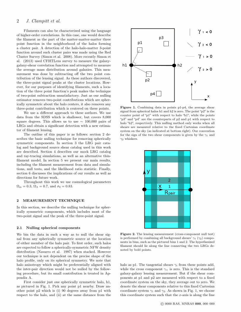
First consider just one spherically symmetric halo, h1,as pictured in Fig. 1. Pick any point p1 nearby. Draw an-other point p2 which is (i) 90 degrees away from p1 withrespect to the halo, and (ii) at the same distance from the

p4

p3

p2

p1

h1 h2

γ1<0

γ1>0

γ2>0

γ2<0

x

y

Figure 1. Combining data in points p1-p4, the average shearsignal from spherical halos h1 and h2 is zero. The point “p2” is thecounter point of “p1” with respect to halo “h1”, while the points“p3” and “p4” are the counterparts of p2 and p1 with respect tohalo “h2”, respectively. This nulling method only works when allshears are measured relative to the fixed Cartesian coordinatesystem on the sky (as indicated at bottom right). Our conventionfor the sign of the two shear components is given by the γ1 andγ2 whiskers.

Figure 2. The lensing measurement (cross-component null test)is performed by combining all background shears’ γ1 (γ2) compo-nents in bins, such as the pictured bins 1 and 2. The hypothesizedfilament should lie along the line connecting the two LRGs de-noted by bold points.

halo as p1. The tangential shears γt from these points add,while the cross component γ× is zero. This is the standardgalaxy-galaxy lensing measurement. But if the shear com-ponents at p1 and p2 are measured with respect to a fixedcoordinate system on the sky, they average out to zero. Wedenote the shear components relative to this fixed Cartesiancoordinate system γ1 and γ2. As shown in Fig. 1, we choosethis coordinate system such that the x-axis is along the line

c© 0000 RAS, MNRAS 000, 000–000

Stacked Filament Lensing 3

connecting h1 and h2 (the two halos) for each halo pair,γ1 < 0 is perpendicular to the x-axis, and γ1 > 0 is parallel.

Now add a second halo, h2. We need to null the h2shear signal in both p1 and p2 as well. To do so, rotate bothpoints by 90 degrees about h2 to make points p3 and p4. Byconstruction, the average γ1 and γ2 shear signal measured atthese four points has no contribution from a spherical haloat h2. Furthermore, one can check that rotating p3 by 90degrees about h1 brings it into p4, so that this set of fourpoints is null with respect to both halos.

Such sets of four points are the building blocks for anumber of possible binning schemes which attempt to nullthe spherically-symmetric halo signal. Note that any set ofbins which exploit this property will necessarily mix scalesrelative to the hypothesized filament. However, since themost likely location for an inter-halo filament is on the lineconnecting the halo pair, we choose bins which will minimizethis mixing of scales. The background shears are separatedinto bands that run parallel or perpendicular to the filamentdirection in Fig. 2. The first two such bins are numbered onthe figure. This binning scheme also exploits the expectedsymmetries about the center of the filament, in both hor-izontal and vertical directions. To verify that a bin doesindeed fulfill the conditions for nulling the spherical signalmentioned above, imagine rotating the part of the bin abovethe Rpair line about either halo, and see that it goes into thesame colored bin in the region below the line. Note also thateach background source is counted twice due to the overlapbetween different bins. This means a naive shape noise ac-counting of errors would underestimate the noise by a factor√

2.In what follows, we describe our measurement proce-

dures of filament lensing. For the halos h1 and h2 in Fig. 1,we use pairs of LRGs (see Sec. 3.1 for details), most of whichare central galaxies of dark matter halos. Implicitly, theabove discussion assumes that the local coordinate systemis defined such that both LRGs lie along the x-axis. Thus,we begin by rotating the RA and DEC coordinates of eachLRG pair and all nearby background galaxies (those withinthe boundaries pictured in Fig. 2) so that the LRG pair al-ways lies along the x-axis. It follows that the y-coordinateof background sources then denotes the distance from theline between the LRG pair. In addition, the source cataloghas shear components (γ′1, γ

′2) which are also defined with

respect to the RA, DEC coordinate system: we simultaneouslyrotate these into (γ1, γ2) components defined with respectto the above (x, y) system.

Then, following the method in Mandelbaum et al.(2013), our lensing observable is given by the shear of back-ground sources γk at the pixel (x, y) times the lensing weightΣcrit. The precise estimator is

∆Σk(x, y; zL) =

∑j

[wj(⟨

Σ−1crit

⟩j

(zL))−1

γk(~xj)

]∑j wj

, (1)

where the summation∑j runs over all the background

galaxies in the pixel (x, y), around all the LRG pairs, theindices k = 1, 2 denote the two components of shear, andthe weight for the j-th galaxy is given by

wj =

[⟨Σ−1

crit

⟩j

(zL)]2

σ2shape + σ2

meas,j

. (2)

We use σshape = 0.32 for the typical intrinsic ellipticitiesand σmeas,j denotes measurement noise on each backgroundgalaxy. Again notice that, when computing the average shearfield, we use the same coordinate system for each LRG pair:taking one LRG at the coordinate origin and taking the x-axis to along the line connecting two LRGs as pictured inFig. 1.

⟨Σ−1

crit

⟩jis the lensing critical density for the j-th

source galaxy, computed by taking into account the photo-metric redshift uncertainty:⟨

Σ−1crit

⟩j

(zL) =

∫ ∞0

dzsΣ−1crit(zL, zs)Pj(zs), (3)

where zL is the redshift of the LRG pair and Pj(zs) is theprobability distribution of photometric redshift for the j-thgalaxy. Note that Σ−1

crit(zL, zs) is computed as a function oflens and source redshifts for the assumed cosmology as

Σ−1crit(zL, zs) =

4πG

c2DA(zL)DA(zL, zs)

DA(zs)(4)

and we set Σ−1crit(zL, zs) = 0 for zs < zL in the computation.

To increase statistics, we will measure the stacked weaklensing signal of filaments as a function of distance y fromthe line connecting the two LRGs. Based on our nullingmethod in Fig. 1, each “p1” point at distance y has its coun-terparts with coordinate values

p1(x, y)→ p2(y,−x), p3(1− x, 1− y), p4(1− y, x− 1) ,(5)

where we set the first LRG position “h1” as the coordinatecenter (x, y) = (0, 0), and we have used the units of Rpair = 1for convenience. Hence we employ the following estimator offilament lensing signal for the a-th distance bin, ya, in Fig. 2:

∆Σfilk (ya) ≡

∑0<xb<0.5

[∆Σk(xb, ya) + ∆Σk(ya,−xb)

+∆Σk(1− xb, 1− ya) + ∆Σk(1− ya, xb − 1)

+∆Σk(xb,−ya) + ∆Σk(ya, xb)

+∆Σk(1− xb, ya − 1) + ∆Σk(1− ya, 1− xb)] , (6)

where ∆Σk(x, y) denotes the k-th component of averageshear at the position (x, y) (see Eq. 1, but note that thesum in the denominator of Eq. 1 runs over all lens-sourcepairs in the bin when plugged into Eq. 6). We use the no-tation ∆Σfil to denote the shear field caused by the grav-itational tidal field due to a filament, with dimensions ofthe surface mass density, but it should not be confused withthe surface mass density used in galaxy-galaxy lensing. Thesummation is over the x-coordinate of the sources, and thesummation range is confined to 0 < xb < 0.5 in order toavoid a double counting of the same background galaxiesin the different quads of points p1, . . . , p4. Note howeverthat the above binning does put each galaxy in two differ-ent bins. The third and fourth lines of Eq. (6) exploit thesymmetry about the line joining the LRG pair, by letting∆Σk(x, y) → ∆Σk(x,−y). Putting each galaxy in two binsin this way does add to our covariance between bins (as wewill later discuss around Fig. 8), but even so there is a gainin information. This is because when a galaxy is put in, say,bin 1 it is averaged together with a different set of galaxiescompared to when it is placed in bin 2.

In the preceding discussion on nulling the LRG lensingsignal, we implicitly assumed that sufficiently many back-ground sources would be found in each pixel (x, y) so that

c© 0000 RAS, MNRAS 000, 000–000


none of p1-4 (Fig. 1) are empty of sources. For example,if there were sources located at p1, p2, and p3, but notp4, the LRG signal would not be nulled. Here we check theassumption that the stacked background source density issuffiently large so as to guarantee that each group of fourpixels has a nulled LRG signal. First, note that we are per-forming a stacked lensing measurement with∼ 135, 000 LRGpairs (see Sec. 3.1), so the total number of sources falling ina given pixel can be estimated as the number for the typ-ical LRG pair times 135,000. Since we will use 8 bins (seeSec. 5) covering 0 < y < Rpair/2 and Rpair > 6 Mpc/h, oursmallest pixel is 3/8 Mpc/h. At the typical lens redshift ofz ∼ 0.3 this physical scale corresponds to an angular scale of∼ 2 arcminutes. The SDSS background source density (seeSec. 3.2) is ∼ 0.25 arcmin−2 at this redshift, so for a singleLRG pair, we would find ∼ 1 galaxy in a single pixel. Then,for the stacked lensing measurement we have approximately100, 000 sources in each pixel, easily satisfying the assump-tion that the stacked, spherically-symmetric LRG shear willbe nulled on average.

2.2 Halo ellipticity

The nulling technique has the extra benefit of mostly re-moving contributions from halo ellipticity, expected to pointalong the line joining the LRG pair. The ellipticity-directioncross-correlation of Lee et al. (2008) has shown that simu-lated dark matter halos tend to point towards other halosin their vicinity. While the intrinsic alignment of LRGs hasbeen measured at a less significant level, the smallness of theintrinsic alignment of the galaxy ellipticity is more likely dueto misalignment of the light and mass profiles (Okumura etal. 2009; Clampitt & Jain 2015), rather than the lack ofalignment between neighboring massive halos. But if we letthe virial radii of these halos be ∆ 6 1 Mpc/h and thepair separation be Rpair > 6 Mpc/h, then the ratio of these∆/Rpair is a small quantity, and we show in Appendix Athat contributions to the signal are highly suppressed asthis ratio gets smaller.

2.3 Jackknife Realizations

We perform the measurement and all null tests by first di-viding up the survey area of 8,000 sq. deg. into 134 approx-imately equal area regions. We then measure each quantitymultiple times with each region omitted in turn to makeN = 134 jackknife realizations. The covariance of the mea-surement (Norberg et al. 2009) is given by

C[∆Σfili ,∆Σfil

j ] =(N − 1)

N

×N∑k=1

[(∆Σfil

i )k −∆Σfili

] [(∆Σfil

j )k −∆Σfilj

](7)

where the mean value is

∆Σfili =

1

N

N∑k=1

(∆Σfili )k , (8)

and (∆Σfili )k denotes the measurement from the k-th real-

ization and the i-th spatial bin. The covariance is measuredfor both components of shear; for clarity we do not denotethe separate shear components in Eqs. 7 and 8.

0.0 0.2 0.4 0.6 0.8 1.0z

0.00

0.01

0.02

0.03

0.04

0.05

0.06

0.07

0.08

P (zL )

P (zs )

Figure 3. The redshift distribution of LRG pairs used as lenses(solid line) and background sources (dashed line).

3 DATA

3.1 Pair catalog

We use the SDSS DR7-Full LRG catalog of Kazin et al.(2010), which contains 105,831 LRGs between 0.16 < z <0.47. The sky coverage is approximately 8,000 sq. deg. Thepair catalog is constructed by choosing each LRG in turn,and finding all neighboring LRGs within a cylinder of phys-ical (or proper) radius 14 Mpc/h and physical line-of-sightdistance ±6 Mpc/h. The redshift distribution of our pairsis in the left panel of Fig. 3. The distribution in line-of-sight distance differences between the pair members isroughly uniform. The cutoff of |∆rlos| < 6 Mpc/h cor-responds roughly to a redshift separation of ∆z < 0.004between pairs. Note that this line-of-sight separation as-sumes the LRG velocity is only due to Hubble flow; inother words, the redshift difference can arise from the differ-ence of line-of-sight peculiar velocities (∆v = 1200 km/s for∆rlos = 6 Mpc/h) even if the two LRGs are in the same dis-tance. This is the so-called redshift space distortion (RSD),and we will discuss the effect of RSD on our weak lensingmeasurements.

We obtain ∼ 135, 000 pairs with the separation cutoffsgiven above: since each LRG can be a member of multiplepairs, this is slightly more than the number of objects asin the original LRG catalog. With Rpair defined to be thephysical projected separation between the LRGs, for pairsbetween 6 Mpc/h < Rpair < 14 Mpc/h we have a distri-bution P (Rpair) which grows very slightly with Rpair. Thevirial radii of these halos are ∼ 0.5− 1.0 Mpc/h, so our se-lection of objects with Rpair > 6 Mpc/h ensures that theseLRGs live in different dark matter halos. We have checkedthat the measurement is insensitive to the choice of physicalvs. comoving distances.

In Fig. 4 we show the stacked shear whiskers forthe smallest Rpair bin; each lens-source pair is optimallyweighted as in Eqs. (1) and (2), and we convert back toγ by assuming fiducial redshifts zL = 0.25 and zs = 0.4. Thetangential shear signal around each member of the LRG pair

c© 0000 RAS, MNRAS 000, 000–000


γ=0.001

1.5 1.0 0.5 0.0 0.5 1.0 1.5

x/Rpair

1.5

1.0

0.5

0.0

0.5

1.0

1.5

y/Rpair

6< Rpair< 10 [Mpc/h]

Figure 4. The stacked shear field for our smallest separationbin, 6 Mpc/h < Rpair < 10 Mpc/h, obtained by stacking thebackground galaxy ellipticities in the same Cartesian coordinatesystem around each LRG pair region (see Fig. 1 and Eq. 1). Thetangential shear signal of the LRG halos is clearly visible. Thegreen box shows the filament measurement region of Fig. 2.

is clearly visible. The nearest whisker to each LRG has mag-nitude ≈ 0.003. Note that due to the large distance betweenwhiskers (0.1Rpair ∼ 1 Mpc/h) even the closest ones to eachhalo are far from the center at ∼ Rvir/2. The dominanceof the LRG halos in these fields motivates our use of thenulling scheme to isolate the relatively tiny filament lensingsignal.

3.2 Background source catalog

The shear catalog is composed of 34.5 million sources, andis nearly identical to that used in Sheldon et al. (2009).The source redshift distribution is shown in Fig. 3, and isobtained by stacking the posterior probability distributionof photometric redshift for each source, P (zs). While thepeak of this source catalog is approximately at the sameredshift as the peak of our LRG pairs, z ∼ 0.35, the sourcedistribution has a substantial tail extending out to higherredshifts. For further details of the shear catalog, see Sheldonet al. (2009).

4 THEORY: THICK- AND THIN-FILAMENTMODELS

We compare the measurement to the following two models,which generally predict “thick” or “thin” filaments, respec-tively: (i) a model obtained based on ray-tracing simulationsor (ii) a one-dimensional string of less massive NFW halos(a collection of NFW halos making up the 1D filament).

4.1 Thick-filament model from ray-tracingsimulations

Here we use a ray-tracing simulation to make a prediction forthe weak lensing signal between LRG pairs. We first selectLRG-like halos in the simulations, and then make pairs andcarry out the same measurement as in Section 2.

4.1.1 Mock catalog of LRG pairs based on ray-tracingsimulations

To model the weak lensing signal of filaments between LRGpairs, we use ray-tracing simulations in Sato et al. (2009)1.Note that they used slightly different cosmological param-eters in the simulations; Ωm = 0.238, ΩΛ = 0.762, andσ8 = 0.76. 2 In brief, the simulations were generated basedon the algorithm in Hamana & Mellier (2001), using N -body simulation outputs of large-scale structure for a ΛCDMcosmology. In this paper, we use the 1000 realizations ofsimulated lensing fields for source redshift zs = 0.6, whereeach realization has an area of 5 × 5 = 25 square degrees.Hence the ray-tracing simulation effectively covers an area of25,000 sq. degrees in total. The lensing fields, convergenceand shear, are provided in the format of 20482 pixels foreach realization. The catalog of halos is also available foreach ray-tracing realization. The halos were identified fromthe N -body simulation output used in each lens plane, usingthe friends-of-friends (FoF) algorithm with linking length of0.2 in units of interparticle spacing. The catalog contains theFoF mass, angular position and redshift for each halo, wherethe halo position was taken from the center-of-mass of FoFmember particles, and the redshift was computed from thedistance in the light-cone simulation.

To build a mock catalog of LRGs, we employ the halooccupation distribution (HOD) method to populate hypo-thetical LRGs into the simulated halos in the range of0.16 6 z 6 0.47, as in the measurements. In this paperwe use the HOD model in Reid & Spergel (2009). Notethat Reid & Spergel (2009) employed the spherical over-density (SO) halo finder with ∆ = 200ρm, and the halomasses of SO and FoF methods might differ by about 10%(Tinker et al. 2008). The HOD consists of the two contri-butions, the mean occupation distribution for central andsatellite galaxies given as a function of host halo mass:〈N〉(M) = 〈Ncen〉(M)[1 + 〈Nsat〉(M)]. For a central LRG,we randomly select halos according to the HOD probabil-ity at the halo mass, which effectively selects all halos atthe high mass end where 〈Ncen〉 ' 1. For satellite LRGs,assuming the Poisson distribution with the mean given by〈Ncen(M)〉〈Nsat〉(M), we generate a random number fromthe Poisson distribution, take the integer number Nsat, andthen populate Nsat LRG(s) into each halo. Note that we donot populate any satellite LRGs into a halo if the halo does

1 http://www.a.phys.nagoya-u.ac.jp/~masanori/HSC/ or avail-able from M. Takada based upon request.2 The σ8 value is smaller than what the recent CMB experimentshave implied, σ8 ' 0.8. Since the filament lensing signal wouldscale with σ8 as ∝ (σ8)4 in the weakly nonlinear regime, basedon the picture of the three-point correlation function, we mightunderestimate the lensing signal by ' 20% if the universe followsσ8 = 0.8.

c© 0000 RAS, MNRAS 000, 000–000

http://www.a.phys.nagoya-u.ac.jp/~masanori/HSC/


x x

6.0Mpc/h<Rpair<10.0Mpc/h

x x

10.0Mpc/h<Rpair<14.0Mpc/h

3.90

3.75

3.60

3.45

3.30

3.15

3.00

2.85

2.70

log 1

0

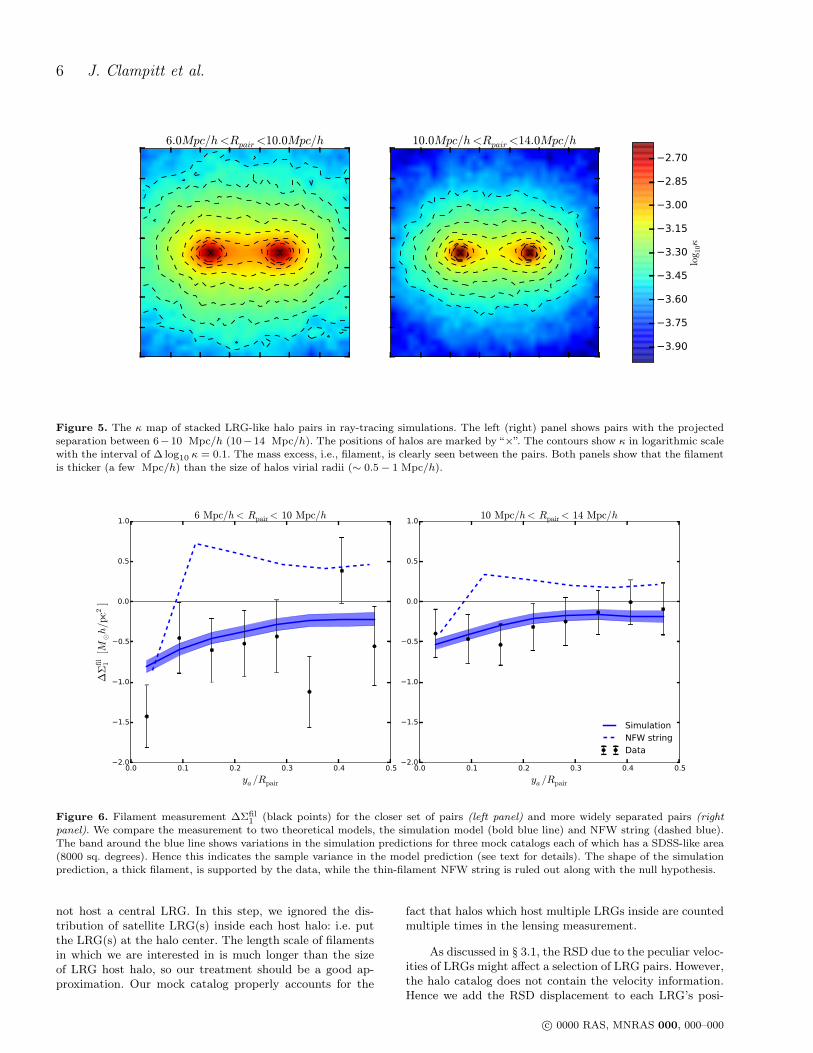
Figure 5. The κ map of stacked LRG-like halo pairs in ray-tracing simulations. The left (right) panel shows pairs with the projectedseparation between 6−10 Mpc/h (10−14 Mpc/h). The positions of halos are marked by “×”. The contours show κ in logarithmic scalewith the interval of ∆ log10 κ = 0.1. The mass excess, i.e., filament, is clearly seen between the pairs. Both panels show that the filamentis thicker (a few Mpc/h) than the size of halos virial radii (∼ 0.5− 1 Mpc/h).

0.0 0.1 0.2 0.3 0.4 0.5

ya /Rpair

2.0

1.5

1.0

0.5

0.0

0.5

1.0

∆Σ

fil

1[M

¯h/p

c2]

6 Mpc/h< Rpair< 10 Mpc/h

0.0 0.1 0.2 0.3 0.4 0.5

ya /Rpair

2.0

1.5

1.0

0.5

0.0

0.5

1.010 Mpc/h< Rpair< 14 Mpc/h

SimulationNFW stringData

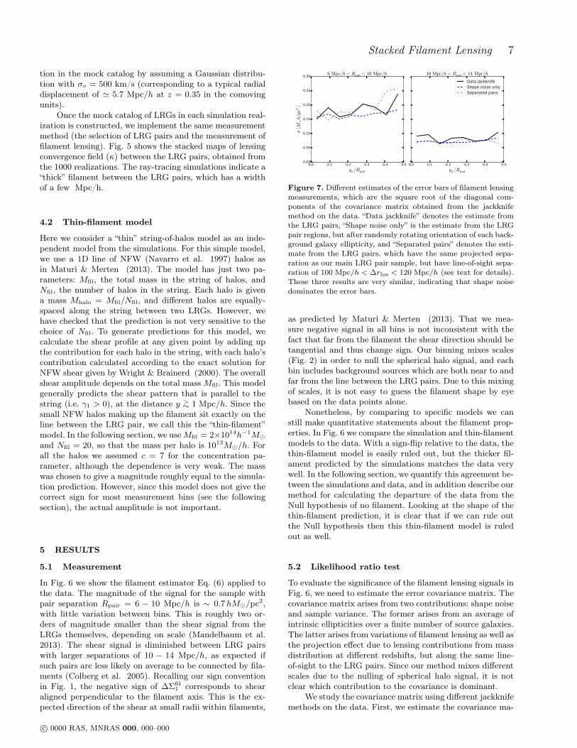
Figure 6. Filament measurement ∆Σfil1 (black points) for the closer set of pairs (left panel) and more widely separated pairs (right

panel). We compare the measurement to two theoretical models, the simulation model (bold blue line) and NFW string (dashed blue).The band around the blue line shows variations in the simulation predictions for three mock catalogs each of which has a SDSS-like area(8000 sq. degrees). Hence this indicates the sample variance in the model prediction (see text for details). The shape of the simulationprediction, a thick filament, is supported by the data, while the thin-filament NFW string is ruled out along with the null hypothesis.

not host a central LRG. In this step, we ignored the dis-tribution of satellite LRG(s) inside each host halo: i.e. putthe LRG(s) at the halo center. The length scale of filamentsin which we are interested in is much longer than the sizeof LRG host halo, so our treatment should be a good ap-proximation. Our mock catalog properly accounts for the

fact that halos which host multiple LRGs inside are countedmultiple times in the lensing measurement.

As discussed in § 3.1, the RSD due to the peculiar veloc-ities of LRGs might affect a selection of LRG pairs. However,the halo catalog does not contain the velocity information.Hence we add the RSD displacement to each LRG’s posi-

c© 0000 RAS, MNRAS 000, 000–000


tion in the mock catalog by assuming a Gaussian distribu-tion with σv = 500 km/s (corresponding to a typical radialdisplacement of ' 5.7 Mpc/h at z = 0.35 in the comovingunits).

Once the mock catalog of LRGs in each simulation real-ization is constructed, we implement the same measurementmethod (the selection of LRG pairs and the measurement offilament lensing). Fig. 5 shows the stacked maps of lensingconvergence field (κ) between the LRG pairs, obtained fromthe 1000 realizations. The ray-tracing simulations indicate a“thick” filament between the LRG pairs, which has a widthof a few Mpc/h.

4.2 Thin-filament model

Here we consider a “thin” string-of-halos model as an inde-pendent model from the simulations. For this simple model,we use a 1D line of NFW (Navarro et al. 1997) halos asin Maturi & Merten (2013). The model has just two pa-rameters: Mfil, the total mass in the string of halos, andNfil, the number of halos in the string. Each halo is givena mass Mhalo = Mfil/Nfil, and different halos are equally-spaced along the string between two LRGs. However, wehave checked that the prediction is not very sensitive to thechoice of Nfil. To generate predictions for this model, wecalculate the shear profile at any given point by adding upthe contribution for each halo in the string, with each halo’scontribution calculated according to the exact solution forNFW shear given by Wright & Brainerd (2000). The overallshear amplitude depends on the total massMfil. This modelgenerally predicts the shear pattern that is parallel to thestring (i.e. γ1 > 0), at the distance y >∼ 1 Mpc/h. Since thesmall NFW halos making up the filament sit exactly on theline between the LRG pair, we call this the “thin-filament”model. In the following section, we useMfil = 2×1014h−1Mand Nfil = 20, so that the mass per halo is 1013M/h. Forall the halos we assumed c = 7 for the concentration pa-rameter, although the dependence is very weak. The masswas chosen to give a magnitude roughly equal to the simula-tion prediction. However, since this model does not give thecorrect sign for most measurement bins (see the followingsection), the actual amplitude is not important.

5 RESULTS

5.1 Measurement

In Fig. 6 we show the filament estimator Eq. (6) applied tothe data. The magnitude of the signal for the sample withpair separation Rpair = 6 − 10 Mpc/h is ∼ 0.7hM/pc2,with little variation between bins. This is roughly two or-ders of magnitude smaller than the shear signal from theLRGs themselves, depending on scale (Mandelbaum et al.2013). The shear signal is diminished between LRG pairswith larger separations of 10 − 14 Mpc/h, as expected ifsuch pairs are less likely on average to be connected by fila-ments (Colberg et al. 2005). Recalling our sign conventionin Fig. 1, the negative sign of ∆Σfil

1 corresponds to shearaligned perpendicular to the filament axis. This is the ex-pected direction of the shear at small radii within filaments,

0.0 0.1 0.2 0.3 0.4 0.5

ya /Rpair

0.00

0.05

0.10

0.15

0.20

0.25

0.30

σ[M

¯h/p

c2]


0.0 0.1 0.2 0.3 0.4 0.5

ya /Rpair


Data jackknifeShape noise onlySeparated pairs

Figure 7. Different estimates of the error bars of filament lensingmeasurements, which are the square root of the diagonal com-ponents of the covariance matrix obtained from the jackknifemethod on the data. “Data jackknife” denotes the estimate fromthe LRG pairs, “Shape noise only” is the estimate from the LRGpair regions, but after randomly rotating orientation of each back-ground galaxy ellipticity, and “Separated pairs” denotes the esti-mate from the LRG pairs, which have the same projected sepa-ration as our main LRG pair sample, but have line-of-sight sepa-ration of 100 Mpc/h < ∆rlos < 120 Mpc/h (see text for details).These three results are very similar, indicating that shape noisedominates the error bars.

as predicted by Maturi & Merten (2013). That we mea-sure negative signal in all bins is not inconsistent with thefact that far from the filament the shear direction should betangential and thus change sign. Our binning mixes scales(Fig. 2) in order to null the spherical halo signal, and eachbin includes background sources which are both near to andfar from the line between the LRG pairs. Due to this mixingof scales, it is not easy to guess the filament shape by eyebased on the data points alone.

Nonetheless, by comparing to specific models we canstill make quantitative statements about the filament prop-erties. In Fig. 6 we compare the simulation and thin-filamentmodels to the data. With a sign-flip relative to the data, thethin-filament model is easily ruled out, but the thicker fil-ament predicted by the simulations matches the data verywell. In the following section, we quantify this agreement be-tween the simulations and data, and in addition describe ourmethod for calculating the departure of the data from theNull hypothesis of no filament. Looking at the shape of thethin-filament prediction, it is clear that if we can rule outthe Null hypothesis then this thin-filament model is ruledout as well.

5.2 Likelihood ratio test

To evaluate the significance of the filament lensing signals inFig. 6, we need to estimate the error covariance matrix. Thecovariance matrix arises from two contributions: shape noiseand sample variance. The former arises from an average ofintrinsic ellipticities over a finite number of source galaxies.The latter arises from variations of filament lensing as well asthe projection effect due to lensing contributions from massdistribution at different redshifts, but along the same line-of-sight to the LRG pairs. Since our method mixes differentscales due to the nulling of spherical halo signal, it is notclear which contribution to the covariance is dominant.

We study the covariance matrix using different jackknifemethods on the data. First, we estimate the covariance ma-

c© 0000 RAS, MNRAS 000, 000–000


Figure 8. (left panel): The normalized covariance matrix of ∆Σfil1 as measured from the data using three variants of the jackknife

method. Bins 1-8 and 9-16 represent the two samples of LRGs with 6− 10 Mpc/h and 10− 14 Mpc/h separation, respectively. (middlepanel): The same, but showing covariance from shape noise alone, obtained by applying a random rotation to source galaxies beforeperforming the measurement. (right panel): The same, but for the Separated pair test from the data.

trix based on the standard method, applying the jackknifemethod to the real LRG pairs (Eq. 7). Secondly, we estimatethe covariance for the shape noise alone; we first randomlyrotate the orientation of each source galaxy ellipticity, re-peat the filament lensing measurement in Eq. (6), and thenestimate the covariance from the jackknife method. The ran-dom orientation erases the lensing signals from both thefilament and the projection effect. We used 20 realizationsto obtain a well-converged covariance estimate. Note thatin this method we keep fixed the positions of source galax-ies, and therefore used the same configurations of tripletsof LRG pairs and source galaxies in the covariance estima-tion. Thirdly, the covariance is estimated from the jackknifemethod using the “separated” LRG pairs, which are selectedsuch that the two LRGs have the same projected separa-tion on the sky as the true LRG pairs, but have a line-of-sight separation of 100 Mpc/h < ∆rlos < 120 Mpc/h (seealso § 5.3 for details). The separated LRG pairs are unlikelyto have filaments between the two LRGs, due to the largethree-dimensional separation, but will include similar lens-ing contributions from the LRG halos and the projectioneffect. Comparing these three covariance matrices revealsthe relative contributions to the covariance from the shapenoise, the filaments and the projection effect.

The diagonal components of the covariance matricesare shown in Fig. 4.2. The three results look very similar,indicating that the shape noise is the dominant source ofthe error bars. Similarly, Fig. 8 compares the off-diagonalcorrelation coefficients of the covariance matrices, rij ≡Cij/

√CiiCjj , estimated from the three jackknife methods

above. The three results again look similar. It should benoted that the shape noise alone causes non-vanishing off-diagonal components, because the filament lensing measure-ments use the same background galaxies multiple times.With the results in Figs. 4.2 and 8, we conclude that theshape noise is the dominant source of the error covariance,and there is no significant contribution of the sample vari-ance. This conclusion is also justified by the mock catalogsof LRG pairs. Since we have the ray-tracing simulation dataof 25,000 sq. degrees in total (see § 4.1.1), we generated 3

SDSS-like mocks each of which has an area of 8,000 sq. de-grees as in the SDSS data. The band around the bold solidline in Fig. 6 denotes the variations in the model predictionsamong the 3 mocks, which show the sample variance contri-bution. The figure clearly shows that the sample variance isvery small compared to the scatter between different bins.Hence in the following we use the covariance estimated fromthe jackknife method on the data (labelled “Data jackknife”in the figures.)

We now move on to an assessment of the significanceof the filament lensing measurement. To do this, we employa “simple-vs-simple” likelihood ratio test to attempt to ruleout the Null hypothesis that there is no excess mass extend-ing between the LRGs, in favor of the Simulation hypothesisthat the mass distribution looks like that in our simulatedLRG pair catalogs. The likelihood ratio is the ratio of thenull likelihood, L0, to the simulation likelihood, Ls:

L0

Ls∝ e−χ

20/2

e−χ2s /2

, (9)

where

χ20 =

∑ij

di(C−1)

ijdj ,

χ2s =

∑ij

(di − dmi )(C−1)

ij(dj − dm

j ) , (10)

C is the covariance matrix estimated from the LRG pairs inFigs. 4.2 and 8, C−1 is the inverse of the matrix, di denotesthe central value of the measurement at the i-th bin, anddmi is the simulation prediction at each bin (the solid lines

in Fig. 6). As our test statistic T we use twice the natu-ral logarithm of the likelihood ratio, dropping an irrelevantconstant from the normalization,

T ≡ χ2s − χ2

0 . (11)

To make a quantitative comparison of the Null and Sim-ulation hypotheses, we generate distributions using “fake”data vectors as follows. Assuming a multi-variate Gaus-sian distribution obeying either L0 ∝ exp(−χ2

0/2) or Ls ∝exp(−χ2

s/2), we generate Monte Carlo realizations of the

c© 0000 RAS, MNRAS 000, 000–000


Figure 9. The comparison of the simulation model (blue hatchedhistogram) with the null hypothesis (green solid histogram) is car-ried out using a likelihood ratio test. The filament measurementfrom data (vertical solid line) can be easily produced if the truemass distribution is similar to that found in the simulation. Incontrast, the null hypothesis of no filament produces a test statis-tic more extreme than the observed measurement in only ∼ 3 outof 106 Monte-Carlo samples, corresponding to a 4.5σ detection.On the other hand, the three null tests, “Cross-component”, “Sep-arated pairs” and “Random points” (see § 5.3 for details) are wellwithin the distribution of null hypothesis.

fake data vector di. Since we used the same covariance ma-trix in both χ2

0 and χ2s , the difference between the distri-

butions is due to the expectation central values: 〈di〉 = 0and 〈di〉 = dm

i for the null and simulation predictions, re-spectively. Fig. 9 shows the distribution of T values (Eq. 11)for the Monte Carlo realizations of Null and Simulation hy-potheses. For example, a “typical” value of the test statisticdrawn at the peak of the Simulation hypothesis histogramfalls in the tail of the Null histogram, and vice-versa.

The results shown in Fig. 9 show that the actual valueof the test statistic T calculated from the data falls near thepeak of the Simulation histogram. In contrast, the data isnot typical if the true model is given by the Null hypothe-sis. The p-value describing the probability that the Null hy-pothesis would produce a test statistic more extreme thanthe data is found to be 0.000003, allowing us to rule outthe Null hypothesis at the 4.5σ confidence level. The valuesof the test statistic for the three null tests (see Sec. 5.3) fallwithin 1σ of the peak of the Null histogram, indicating thesetests pass.

5.3 Null tests: Separated pairs, Cross-component,and Random points

In order to validate the measurement in the previous sec-tions, we perform three null tests on the data. For all nulltests, we repeat the measurement of our Eq. (6) estimatorfor ∆Σfil

1 using the same jackknife regions. First, the Sep-arated pair test involves using two LRGs at the “h1” and“h2” positions of Fig. 1, but with line-of-sight separation100 Mpc/h < ∆rlos < 120 Mpc/h. The 3D distance of suchpairs is so large that we expect no excess mass to build up

between them. For the lens redshift zL, we use the averageof the two LRG redshifts. The result is shown in Fig. 10(green diamonds) and is consistent with the Null hypothe-sis (Fig. 9). This test shows that the spherically symmetricshear signal from both LRGs in the measurement is trulynulled, as claimed.

This null test measurement has a further use in veri-fying one of our approximations in Sec. 5.2. We assumedthat the data covariance is a fair approximation to the Nullhypothesis covariance, which should include all sources ofnoise which would appear if the Null hypothesis were true.This includes shape noise, as well as residual noise from theuncancelled part of the LRG halo signal and other mass dis-tributions which are not completely nulled by our estimator,Eq. (6). It should not include noise from variations in thepurported filament itself, which would not be present giventhe Null hypothesis. We find the Separated pair jackknifecovariance differs only slightly from the filament covarianceitself (Fig. 8), and the detection significance shifts by lessthan 1σ when using this covariance for the Null hypothesis.

Second, as in tangential shear measurements, wherethe cross-component of shear rotated by 45 has no first-order contribution from gravitational lensing, our cross-component (the ∆Σfil

2 component of Eq. 6) has no contri-bution from a filament. This statement holds as long as thestacked mass distribution around the LRG pairs has reflec-tion symmetry about the line joining the pairs. For sucha mass distribution, in the Cartesian coordinate system ofFig. 1, γ2(y) = −γ2(−y). Since background sources at y arealways put in the same bin with sources at −y, (see Fig. 2),∆Σfil

2 = 0 on average. This is what we find in Fig. 10, wherethe magenta triangles show the result of this null test. Againthe result for the test statistic in Fig. 9 is consistent withthe Null hypothesis.

For the Random points test, we repeat the measure-ment on ∼ 10 times as many random points with the samedistribution in z and Rpair as the pair catalog. The randompositions and orientations used in this test should stack in-dividual halos and filaments such that the final mass distri-bution is isotropic, and thus nulled by our procedure. Theresult is shown in Fig. 10 (blue circles). Like the others thistest passes, as shown in Fig. 9.

Finally, we perform one more check, a variation on theSeparated pair test, again using LRGs with line-of-sight sep-aration ∆rlos = 100− 120 Mpc/h. The difference is that wenow select the LRGs that overlap in projection, with sep-arations Rpair between 0.1 and 2 Mpc/h. We then repeatthe measurement as before, using the same estimator of fil-ament signal. Since the range of Rpair does not match ourother tests (or the filament measurement), it is not straight-forward to directly plot the results of this test on Fig. 9 or10. Instead we simply check that the reduced χ2 statisticis consistent with the null hypothesis. Indeed, with reducedχ2 = 4/8 the result is easily consistent with the null expec-tation.

6 DISCUSSION

We have presented a technique for the statistical measure-ment of properties of the dark matter filaments linking closepairs of galaxies and clusters. Our method uses an empiri-

c© 0000 RAS, MNRAS 000, 000–000


0.0 0.1 0.2 0.3 0.4 0.5

ya /Rpair

2.0

1.5

1.0

0.5

0.0

0.5

1.0

∆Σ

fil

[M¯h/p

c2]

6.0 Mpc/h< Rpair< 10.0 Mpc/h

0.0 0.1 0.2 0.3 0.4 0.5

ya /Rpair

2.0

1.5

1.0

0.5

0.0

0.5

1.010.0 Mpc/h< Rpair< 14.0 Mpc/h

Separated pair testRandom points testCross-component test

Figure 10. Same as Fig. 6, but showing the results of three null tests (as labelled in the legend). The separated pair test, random pointstest, and cross-component test are all consistent with the null hypothesis. Note that the null result for the separated pair test shows thatour estimator does successfully null the spherically symmetric signal from the LRG halos.

cal approach which relies on few assumptions to cancel outthe contribution of spherical halos in the data. Applying thistechnique to pairs of LRGs in SDSS we detect residual shearpatterns of magnitude ∼ 10−4, about one order of magni-tude smaller than the LRG halo signal at 5 Mpc/h from thehalo center, and two orders of magnitude smaller than theLRG signal at its virial radius. Employing a likelihood ratiotest, we attribute this signal to filamentary structures with adetection significance higher than 4σ. The small signal, thepossible systematics in SDSS imaging, and the dominance ofthe LRG halos make the measurement especially challeng-ing. We have carried out several null tests which provideevidence that our nulling technique is robust and that sys-tematic errors are minimized. Applying the same LRG pairselection and lensing estimator to simulations, we find an ex-cellent match with the data. With a width of a few Mpc/hthe stacked filament shape is determined to be thicker thanthe LRG halos at its end points.

There are several approximations and sources of errorin our analysis.

• The stacking of hundreds of thousands of LRG pairsleads to a smearing of the mass distribution. This meansthat we cannot make definitive statements about the typical(individual) filament structures in the universe, in particularthe limits we obtain on the thickness of the filament onlyapply to the stacked profile.• The binning scheme we use to null out the contribu-

tion of spherical halos also nulls part of the signal from thefilaments we seek to measure. In this sense our estimator issub-optimal (though it would be challenging to construct anoptimal estimator while subtracting the LRG halo signal).• The calibration of the shear, which relies on a correc-

tion for the smearing due to the PSF, introduces a redshiftdependent bias that propagates to the filament mass esti-mate. Uncertainties in the photometric redshifts of back-ground galaxies have a similar effect. Both are below the 10percent level and smaller than our statistical uncertainties.• Redshift space distortions: the line of sight separation

of the LRGs is uncertain owing to their relative peculiarvelocity. We have attempted to account for it by addingRSD to the simulations (see Sec. 4.1.1).• The inevitable contamination of the LRG sample with

other galaxies and stars leads to a dilution of the signal.This should be controlled to better than the 10% level.

In future work several improvements can be made thataddress the above points. In addition, forward modeling ofthe measurement can be done using simulations and the halomodel, so that comparisons can be made without use of ournulling technique. Such an approach may allow for more de-tailed tests of the halo model and of filamentary properties,though care will need to be exercised to distinguish system-atic errors. Finally, an interesting complement to our studyis to compare the mass distribution inferred from lensingshears with the distribution of foreground galaxies and hotgas.

ACKNOWLEDGMENTS

We would like to thank Gary Bernstein, Sarah Bridle,Jörg Dietrich, Mike Jarvis, Elisabeth Krause, Ravi Sheth,Yuanyuan Zhang and especially Rachel Mandelbaum forhelpful discussions and comments. We are very grateful toErin Sheldon for the use of his SDSS shear catalogs andto Tomasz Kacprzak for related collaborative work. BJ andMT also thank the Aspen Center for Physics and NSF Grant#1066293, for their warm hospitality when part of this workwas done. BJ and JC are partially supported by Departmentof Energy grant de-sc0007901. MT is supported by WorldPremier International Research Center Initiative (WPI Ini-tiative), MEXT, Japan, by the FIRST program “SubaruMeasurements of Images and Redshifts (SuMIRe)”, CSTP,Japan, by Grant-in-Aid for Scientific Research from theJSPS Promotion of Science (No. 23340061 and 26610058),and by MEXT Grant-in-Aid for Scientific Research on Inno-vative Areas (No. 15H05893 and 15K21733). HM was sup-

c© 0000 RAS, MNRAS 000, 000–000

http://arxiv.org/abs/de-sc/0007901


ported in part by Japan Society for the Promotion of Science(JSPS) Research Fellowships for Young Scientists. HM wassupported in part by the Jet Propulsion Laboratory, Cal-ifornia Institute of Technology, under a contract with theNational Aeronautics and Space Administration.

APPENDIX A: HALO ELLIPTICITY

In order to show that the contribution from halo ellipticityis small, we consider a very simple model which is even lessspherical than an elliptical halo. Thus, if the shear from thismodel is negligible, then so is shear from elliptical halos.We take two point masses labelled E1 and E2 on Fig. A1.These are each separated from the halo center by ∆ . Rvir.The outermost square region pictured corresponds to thetop square of Fig. 1, with side length Rpair.

On the left panel of Fig. A1 we extend two lines fromE1 which are both 45 degrees from the horizontal axis. Withour shear sign convention (Fig. 1), these lines describe pointswhere the shear from E1 is purely γ2, i.e., these lines arethe zeros of γ1. Thus, points which are on opposite sides ofand equidistant from these lines have a net contribution ofγ1 = 0. As a result, the net γ1 shear when summed over allgalaxies in regions A and A’ is zero. In the same way, regionsB and B’ sum to zero.

Likewise, on the right panel we draw a line from E2which is 45 degrees from the vertical, and the net γ1 shearin C and C’ is zero. A final cancellation occurs in regions Dand D’, where the positive γ1 shear from E1 in D cancels thenegative shear from E2 in D’. The net shear from these twopoint masses is then given by the remaining regions, labelled+γ and −γ. These two regions do not cancel perfectly, butit is clear that (i) these regions nearly cancel: while the +γregion is slightly closer to E1 than the −γ region is to E2, inarea, the +γ region is slightly smaller; (ii) the size of theseimperfectly cancelled regions shrinks rapidly as ∆/Rpair getssmaller. The upper bound is

∆/Rpair 6Rvir

Rpair=

1 Mpc/h

6 Mpc/h, (A1)

but most of our LRG pairs have smaller virial radii andlarger pair separation. Furthermore, the density profile ofhalos falls off quickly, so that relatively little of the mass isdisplaced an entire virial radius from the center.

REFERENCES

Cautun, M., van de Weygaert, R., Jones, B. J. T., & Frenk,C. S. 2014, arXiv:1401.7866

Clampitt, J., Jain, B., arXiv:1506.03536Colberg, J. M., Krughoff, K. S., & Connolly, A. J. 2005,MNRAS, 359, 272

Dietrich, J. P., Werner, N., Clowe, D., et al. 2012, Nature(London), 487, 202

Hamana, T., Mellier, Y., 2001, MNRAS, 327, 169Jauzac, M., Jullo, E., Kneib, J.-P., et al. 2012, MNRAS,426, 3369

Kazin, E. A., Blanton, M. R., Scoccimarro, R., et al. 2010,ApJ, 710, 1444

Lee, J., Springel, V., Pen, U.-L., & Lemson, G. 2008, MN-RAS, 389, 1266

Figure A1. As an extreme model of halo ellipticity, we considerthe shear from point masses E1 and E2. The two panels show thesame region twice: the left panel highlights the contribution fromE1, and the right that from E2. The net γ1 shear (with the signconvention of Fig. 1) cancels in regions A and A’, B and B’, etc.(See the text for the details.) The size of the uncancelled regions,+γ and −γ, shrinks rapidly with the small number ∆/Rpair 61/6, showing that contributions from halo ellipticity are highlysuppressed in our measurement.

Mandelbaum, R., Slosar, A., Baldauf, T., et al. 2013, MN-RAS, 432, 1544

Maturi, M., & Merten, J. 2013, arXiv:1306.0015Mead, J. M. G., King, L. J., & McCarthy, I. G. 2010, MN-RAS, 401, 2257

Navarro, J. F., Frenk, C. S., & White, S. D. M. 1997, ApJ,490, 493

Norberg, P., Baugh, C. M., Gaztañaga, E., & Croton, D. J.2009, MNRAS, 396, 19

Okumura, T., Jing, Y. P., & Li, C. 2009, ApJ, 694, 214Reid, B. A., & Spergel, D. N. 2009, ApJ, 698, 143Sato, M., Hamana, T., Takahashi, R., et al. 2009, ApJ, 701,945

Sheldon, E. S., Johnston, D. E., Scranton, R., et al. 2009,ApJ, 703, 2217

Simon, P., Watts, P., Schneider, P., et al. 2008, A&A, 479,655

Simon, P., et al., 2013, MNRAS, 430, 2476Sousbie, T. 2011, MNRAS, 414, 350Tinker, J., Kravtsov, A. V., Klypin, A., et al. 2008, ApJ,688, 709

Wright, C. O., & Brainerd, T. G. 2000, ApJ, 534, 34Zhang, Y., Dietrich, J. P., McKay, T. A., Sheldon, E. S., &Nguyen, A. T. Q. 2013, arXiv:1304.6696

c© 0000 RAS, MNRAS 000, 000–000

http://arxiv.org/abs/1401.7866




Documents

Detection of Stacked Filament Lensing Between SDSS