Determinants of science graduates labour market success* · Determinants of science graduates labour market success* Tomasz Gajderowicz (University of Warsaw) Gabriela Grotkowska

Determinants of science graduates labour market success*

Tomasz Gajderowicz (University of Warsaw)

Gabriela Grotkowska (University of Warsaw)

Leszek Wincenciak (University of Warsaw)

12.09.2011

Abstract

The article studies the problem of success in the labour market entry of higher education

graduates in the European perspective. The core of the analysis is the study of determinants of

widely defined labour market success. Differences between countries and study domains are

analysed in the aspects of the influence of various socio-demographic characteristics as well

as market environment and process of learning, modes of teaching and study programmes

characteristics. Specifically, the Science domain is taken under focus. Data used in the

analysis comes from two special surveys of European research projects REFLEX and

HEGESCO. The research shows important role of factors related to study programmes modes

and processes as well as individual graduates‟ study and early work-related experience.

Key words: labour market success, graduates

______________________________

* This paper was prepared as a result of DEHEMS project. This project has been funded with

support from the European Commission. This publication [communication] reflects the views

only of the author, and the Commission cannot be held responsible for any use which may be

made of the information contained therein.

2

Introduction

In the last decade the number of students in the EU-27 grew by almost 30% (from 15 million

in 1998 up to more than 19 million in 2009). Most dynamic changes occurred in the new

member states of the Central and Eastern Europe, where number of students grew two- or

even threefold, but positive trend prevailed in all EU member countries. As a result, the

problem of tertiary education graduates‟ employability became an central issue in labour

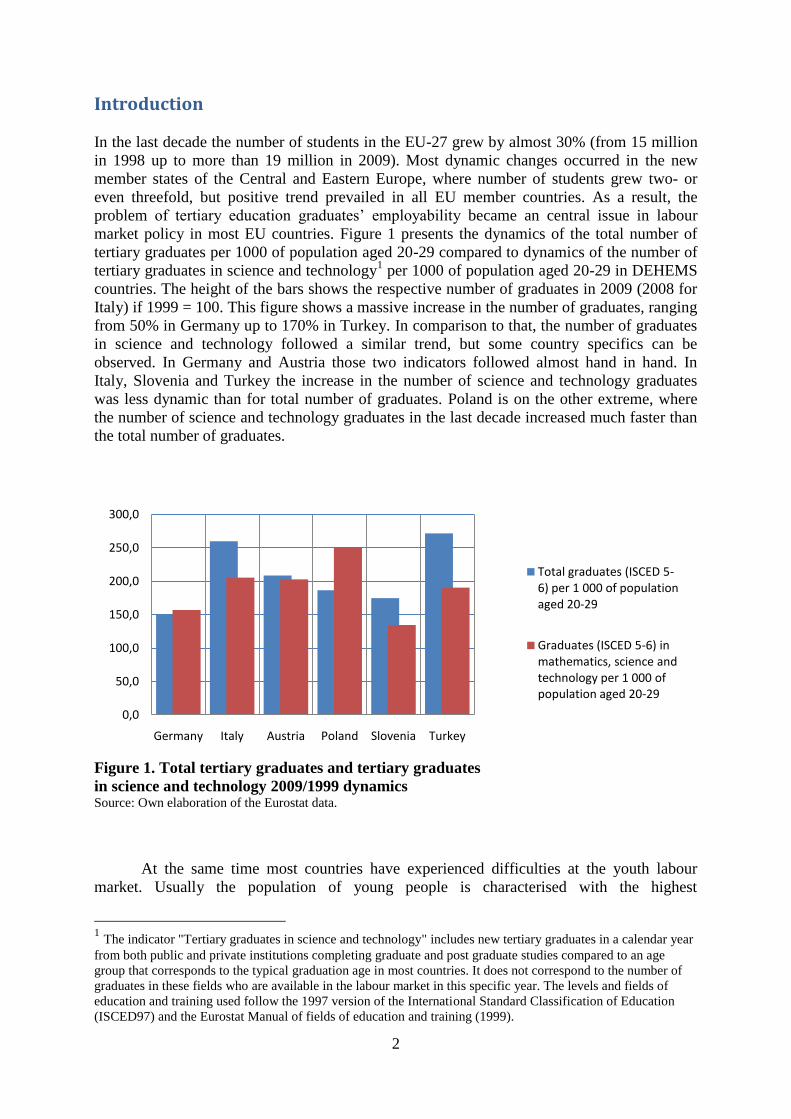
market policy in most EU countries. Figure 1 presents the dynamics of the total number of

tertiary graduates per 1000 of population aged 20-29 compared to dynamics of the number of

tertiary graduates in science and technology1 per 1000 of population aged 20-29 in DEHEMS

countries. The height of the bars shows the respective number of graduates in 2009 (2008 for

Italy) if 1999 = 100. This figure shows a massive increase in the number of graduates, ranging

from 50% in Germany up to 170% in Turkey. In comparison to that, the number of graduates

in science and technology followed a similar trend, but some country specifics can be

observed. In Germany and Austria those two indicators followed almost hand in hand. In

Italy, Slovenia and Turkey the increase in the number of science and technology graduates

was less dynamic than for total number of graduates. Poland is on the other extreme, where

the number of science and technology graduates in the last decade increased much faster than

the total number of graduates.

Figure 1. Total tertiary graduates and tertiary graduates

in science and technology 2009/1999 dynamics Source: Own elaboration of the Eurostat data.

At the same time most countries have experienced difficulties at the youth labour

market. Usually the population of young people is characterised with the highest

1 The indicator "Tertiary graduates in science and technology" includes new tertiary graduates in a calendar year

from both public and private institutions completing graduate and post graduate studies compared to an age

group that corresponds to the typical graduation age in most countries. It does not correspond to the number of

graduates in these fields who are available in the labour market in this specific year. The levels and fields of

education and training used follow the 1997 version of the International Standard Classification of Education

(ISCED97) and the Eurostat Manual of fields of education and training (1999).

0,0

50,0

100,0

150,0

200,0

250,0

300,0

Germany Italy Austria Poland Slovenia Turkey

Total graduates (ISCED 5-6) per 1 000 of population aged 20-29

Graduates (ISCED 5-6) in mathematics, science and technology per 1 000 of population aged 20-29

3

unemployment rates and the lowest employment rates. At the same time, it is a group

suffering from lowest quality of employment (with relatively low wages and low level of

employment security). It poses a question of efficiency of education process and its impact on

employment and wage profiles.

The labour market success may be understood in many different ways. The measure

mostly often used for labour market success is a fact of carrying out a paid work. It is

regarded as an indicator of workers‟ attractiveness from the labour demand point of view and

of the match of their education profile to market requirements. However such definition of a

labour market success posses further difficulties: is an university graduate that failed to find

work in her occupation and work for a three hours a week as a babysitter successful on the

labour market? According to the ILO definitions, she will be recognised as an employed

person. For assessing labour market success not only the fact of work, but also its time and

quality should be taken for an account (the problem has been discussed by Kalleberg et al.

2000 and recently by Howell and Diallo, 2008). Only if we take into consideration

characteristics of job, we‟ll be capable of shed some light of determinants of the actual labour

market success.

1. Graduates’ of Science domain socio-biographic background

In all six DEHEMS Project countries (Austria, Germany, Italy, Poland, Slovenia and Turkey,

referred to as DEHEMS countries for short further on) students of Science domain constitute

a very different part of all students population. The largest share is observed in Germany

where every sixth student is studying a programme which belongs to Science domain. On the

other extreme we have Slovenia with only 4,6%, which means that this study domain is not

that much popular among young Slovenians. Detailed structure of students in the Science

domain for six DEHEMS countries is shown in the table below.

Table 1. Share of Science domain students in DEHEMS countries

Austria Germany Italy Poland Slovenia Turkey

Life sciences (ISC 42) 3.1 3.7 3.5 1.9 1.4 1.7

Physical sciences (ISC 44) 2.3 4.8 1.3 1.3 1.1 3.6

Mathematics and statistics (ISC 46) 0.8 2.9 0.8 0.8 0.4 2.3

Computing (ISC 48) 7.1 5.0 1.3 3.4 1.7 1.1

Total 13.3 16.4 6.9 7.4 4.6 8.7 Source: OECD and Statistical Office of the Republic of Slovenia, as of 2009.

In all DEHEMS countries except for Italy, Science domain is dominated by male students.

This observation is contrasting with the fact that generally for all study fields share of female

students is higher than 50% (with the exception of Turkey, probably to traditional and cultural

reasons). In Austria the scale of feminization of the Science domain is lowest with a share of

women 33.1% only. The most man-dominated study field is not surprisingly Computing (ISC

48). Detailed figures for feminization are shown in table 2.

Table 2. Share of women in the population of Science domain students in DEHEMS countries

Austria Germany Italy Poland Slovenia Turkey

Life sciences (ISC 42) 67.3 66.6 70.1 74.0 71.2 62.3

Physical sciences (ISC 44) 34.6 43.7 38.9 65.8 44.4 43.3

Mathematics and statistics (ISC 46) 37.6 64.3 54.9 70.0 59.4 45.8

4

Computing (ISC 48) 17.4 15.6 15.9 18.6 7.8 24.0

Total over Science (ISC 400) 33.1 44.1 52.5 47.0 40.5 45.3

Total over all fields of study 52.8 55.4 58.3 65.6 64.3 46.4 Source: OECD and Statistical Office of the Republic of Slovenia, as of 2009.

2. Labour market success: key concepts

Traditionally, labour market success after graduation is interpreted in terms of possessing paid

employment. Therefore a synthetic measure of success in given study discipline would be an

aggregated employment rate. This traditional approach, although still useful is however not

sufficient to describe various aspects of the term – “success” and its necessarily subjective

nature. Given differences in preferences, one can observe different aspects being perceived as

success by different individuals. Furthermore, the idea of success can be related to socio-

demographic background of individuals, their values and beliefs and economic context

(business cycle effect). Other aspects of success that can be taken under consideration are

therefore:

- Types of employment contracts: short-term employment contracts do not give

appropriate level of security;

- Employment stability: frequent job changes prevent from accumulating job-specific

human capital;

- Wage level: low wages provide low return to education and decrease the incentives to

acquire human capital through both formal education and on-the-job training;

- Human capital accumulation: knowledge cumulated by work experience is a valuable

asset itself;

- Utilization of skills and knowledge acquired during education: allows to effectively

use the skills and knowledge provided by HEI and to develop them by job experience;

- Personal development: important for subjective perception of overall development;

- Career perspectives: starting with low position but with open possibilities might be

more important than having relatively high position from the beginning but with some

form of glass ceiling;

- Degree in which actual job matches graduate‟s expectations: important for subjective

perception of satisfaction;

- General satisfaction: work-life balance, which gives enough time to spend with the

family and enough income to enjoy consumption of variety of goods and services.

Labour market success can be interpreted in many ways, in terms of job satisfaction, job

security, appropriate earnings, work autonomy and independence, work being a challenge and

opportunity to develop skills and knowledge, ability to balance job duties with family and

social life, possesing a job matching the skills and knowledge gained during studies. The

problem of operationalization of the labour market success of graduates is described in section

4. Next section describes various characteristics of the first employment of science graduates.

3. Transition of science graduates into labour market

3.1. Labour market status

The most standard approach to the labour market success relies on looking at the labour

market status of graduates. When asked about their current status, 91,4% of graduates of

5

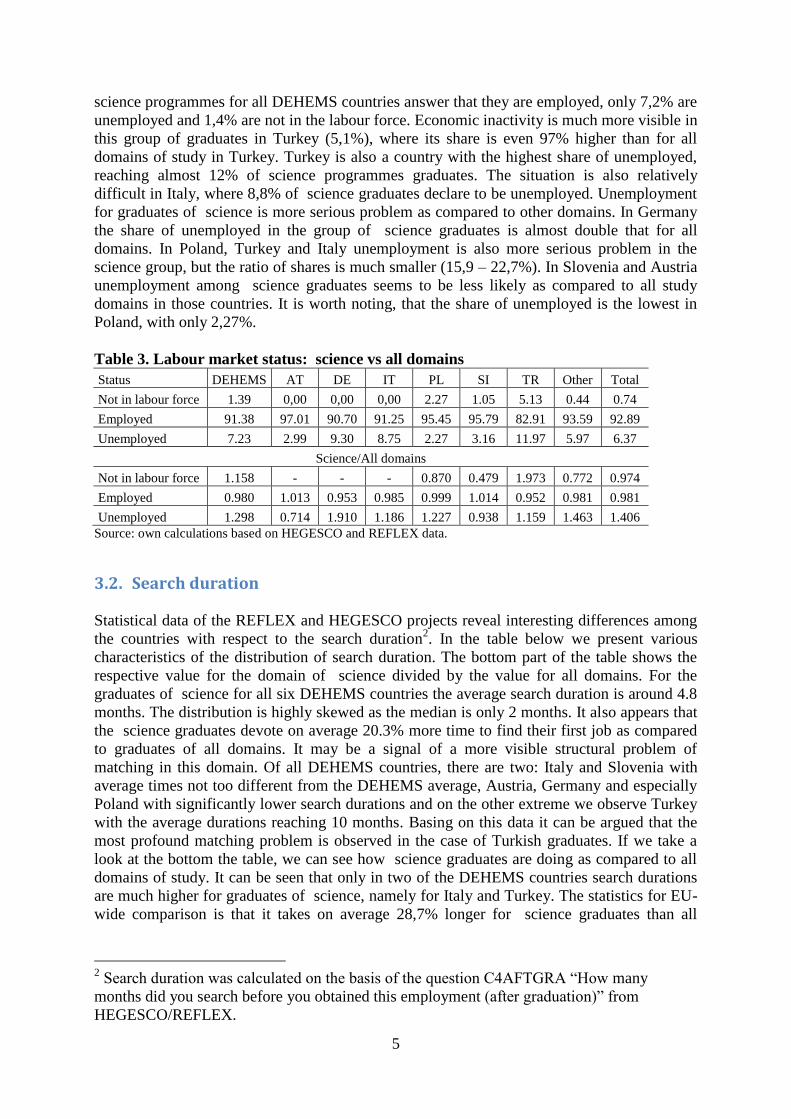
science programmes for all DEHEMS countries answer that they are employed, only 7,2% are

unemployed and 1,4% are not in the labour force. Economic inactivity is much more visible in

this group of graduates in Turkey (5,1%), where its share is even 97% higher than for all

domains of study in Turkey. Turkey is also a country with the highest share of unemployed,

reaching almost 12% of science programmes graduates. The situation is also relatively

difficult in Italy, where 8,8% of science graduates declare to be unemployed. Unemployment

for graduates of science is more serious problem as compared to other domains. In Germany

the share of unemployed in the group of science graduates is almost double that for all

domains. In Poland, Turkey and Italy unemployment is also more serious problem in the

science group, but the ratio of shares is much smaller (15,9 – 22,7%). In Slovenia and Austria

unemployment among science graduates seems to be less likely as compared to all study

domains in those countries. It is worth noting, that the share of unemployed is the lowest in

Poland, with only 2,27%.

Table 3. Labour market status: science vs all domains

Status DEHEMS AT DE IT PL SI TR Other Total

Not in labour force 1.39 0,00 0,00 0,00 2.27 1.05 5.13 0.44 0.74

Employed 91.38 97.01 90.70 91.25 95.45 95.79 82.91 93.59 92.89

Unemployed 7.23 2.99 9.30 8.75 2.27 3.16 11.97 5.97 6.37

Science/All domains

Not in labour force 1.158 - - - 0.870 0.479 1.973 0.772 0.974

Employed 0.980 1.013 0.953 0.985 0.999 1.014 0.952 0.981 0.981

Unemployed 1.298 0.714 1.910 1.186 1.227 0.938 1.159 1.463 1.406

Source: own calculations based on HEGESCO and REFLEX data.

3.2. Search duration

Statistical data of the REFLEX and HEGESCO projects reveal interesting differences among

the countries with respect to the search duration2. In the table below we present various

characteristics of the distribution of search duration. The bottom part of the table shows the

respective value for the domain of science divided by the value for all domains. For the

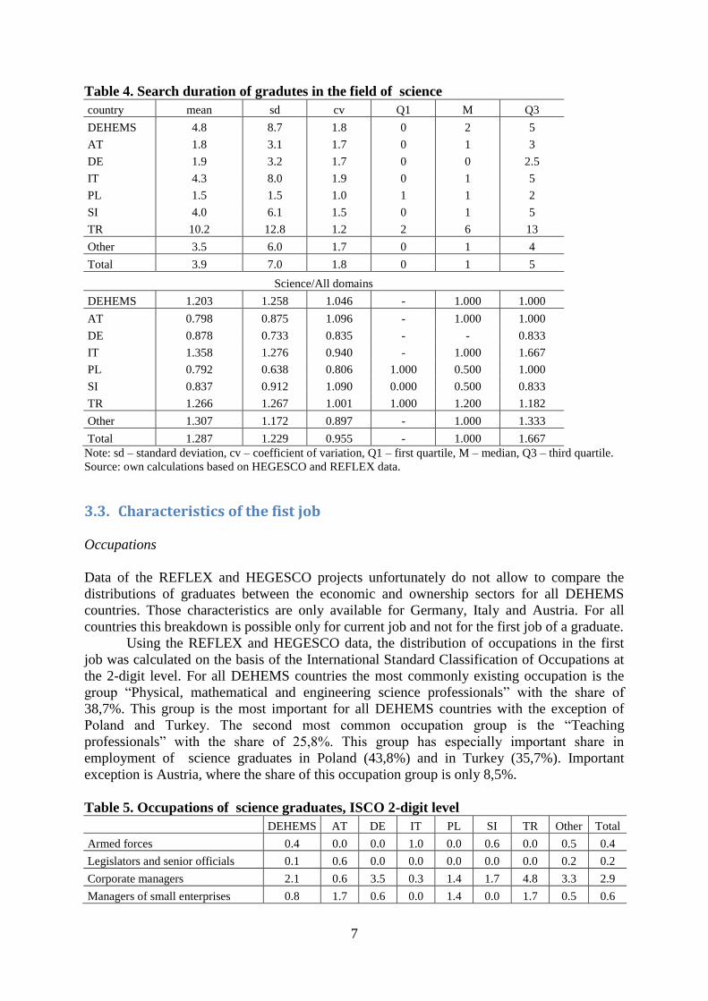
graduates of science for all six DEHEMS countries the average search duration is around 4.8

months. The distribution is highly skewed as the median is only 2 months. It also appears that

the science graduates devote on average 20.3% more time to find their first job as compared

to graduates of all domains. It may be a signal of a more visible structural problem of

matching in this domain. Of all DEHEMS countries, there are two: Italy and Slovenia with

average times not too different from the DEHEMS average, Austria, Germany and especially

Poland with significantly lower search durations and on the other extreme we observe Turkey

with the average durations reaching 10 months. Basing on this data it can be argued that the

most profound matching problem is observed in the case of Turkish graduates. If we take a

look at the bottom the table, we can see how science graduates are doing as compared to all

domains of study. It can be seen that only in two of the DEHEMS countries search durations

are much higher for graduates of science, namely for Italy and Turkey. The statistics for EU-

wide comparison is that it takes on average 28,7% longer for science graduates than all

2 Search duration was calculated on the basis of the question C4AFTGRA “How many

months did you search before you obtained this employment (after graduation)” from

HEGESCO/REFLEX.

6

graduates to find their first jobs. Italy is an example where the science graduates situation is

relatively the worst with respect to search durations.

7

Table 4. Search duration of gradutes in the field of science

country mean sd cv Q1 M Q3

DEHEMS 4.8 8.7 1.8 0 2 5

AT 1.8 3.1 1.7 0 1 3

DE 1.9 3.2 1.7 0 0 2.5

IT 4.3 8.0 1.9 0 1 5

PL 1.5 1.5 1.0 1 1 2

SI 4.0 6.1 1.5 0 1 5

TR 10.2 12.8 1.2 2 6 13

Other 3.5 6.0 1.7 0 1 4

Total 3.9 7.0 1.8 0 1 5

Science/All domains

DEHEMS 1.203 1.258 1.046 - 1.000 1.000

AT 0.798 0.875 1.096 - 1.000 1.000

DE 0.878 0.733 0.835 - - 0.833

IT 1.358 1.276 0.940 - 1.000 1.667

PL 0.792 0.638 0.806 1.000 0.500 1.000

SI 0.837 0.912 1.090 0.000 0.500 0.833

TR 1.266 1.267 1.001 1.000 1.200 1.182

Other 1.307 1.172 0.897 - 1.000 1.333

Total 1.287 1.229 0.955 - 1.000 1.667

Note: sd – standard deviation, cv – coefficient of variation, Q1 – first quartile, M – median, Q3 – third quartile.


3.3. Characteristics of the fist job

Occupations

Data of the REFLEX and HEGESCO projects unfortunately do not allow to compare the

distributions of graduates between the economic and ownership sectors for all DEHEMS

countries. Those characteristics are only available for Germany, Italy and Austria. For all

countries this breakdown is possible only for current job and not for the first job of a graduate.

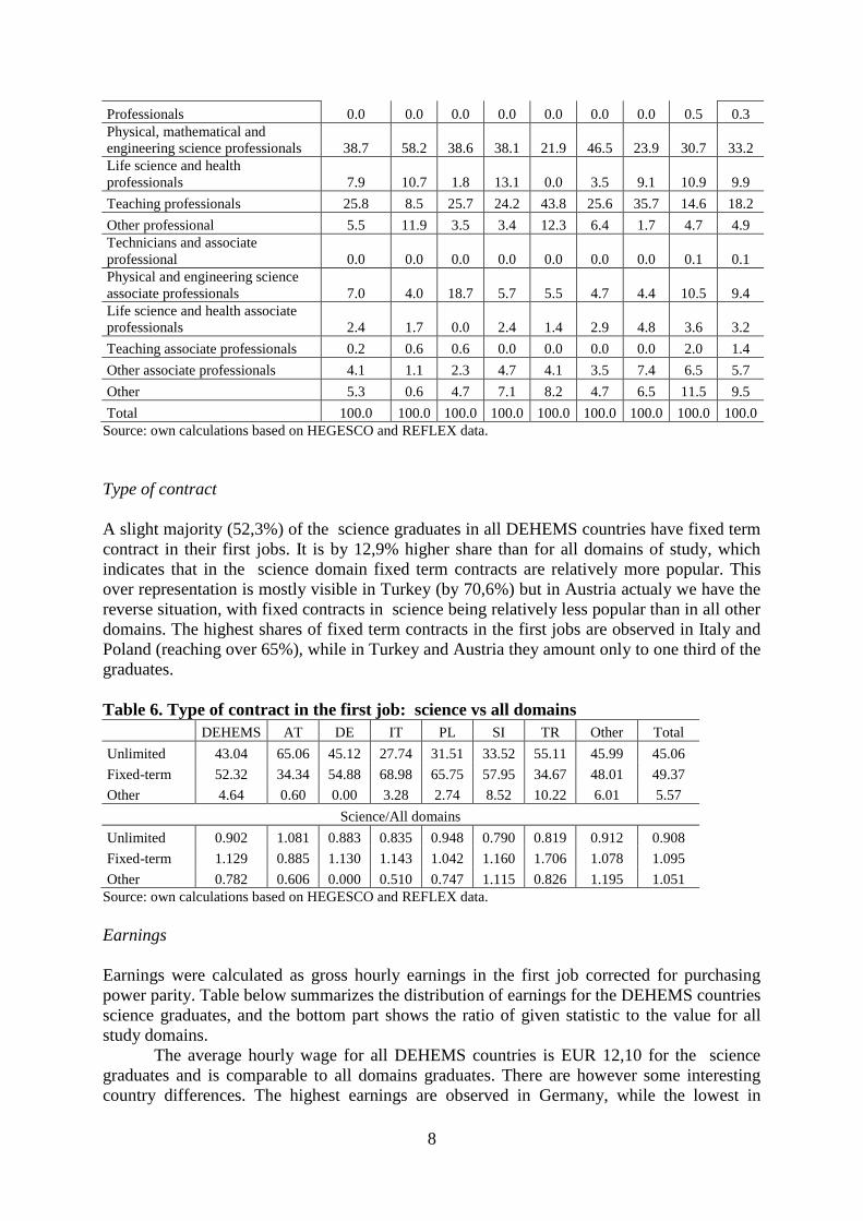
Using the REFLEX and HEGESCO data, the distribution of occupations in the first

job was calculated on the basis of the International Standard Classification of Occupations at

the 2-digit level. For all DEHEMS countries the most commonly existing occupation is the

group “Physical, mathematical and engineering science professionals” with the share of

38,7%. This group is the most important for all DEHEMS countries with the exception of

Poland and Turkey. The second most common occupation group is the “Teaching

professionals” with the share of 25,8%. This group has especially important share in

employment of science graduates in Poland (43,8%) and in Turkey (35,7%). Important

exception is Austria, where the share of this occupation group is only 8,5%.

Table 5. Occupations of science graduates, ISCO 2-digit level

DEHEMS AT DE IT PL SI TR Other Total

Armed forces 0.4 0.0 0.0 1.0 0.0 0.6 0.0 0.5 0.4

Legislators and senior officials 0.1 0.6 0.0 0.0 0.0 0.0 0.0 0.2 0.2

Corporate managers 2.1 0.6 3.5 0.3 1.4 1.7 4.8 3.3 2.9

Managers of small enterprises 0.8 1.7 0.6 0.0 1.4 0.0 1.7 0.5 0.6

8

Professionals 0.0 0.0 0.0 0.0 0.0 0.0 0.0 0.5 0.3

Physical, mathematical and

engineering science professionals 38.7 58.2 38.6 38.1 21.9 46.5 23.9 30.7 33.2

Life science and health

professionals 7.9 10.7 1.8 13.1 0.0 3.5 9.1 10.9 9.9

Teaching professionals 25.8 8.5 25.7 24.2 43.8 25.6 35.7 14.6 18.2

Other professional 5.5 11.9 3.5 3.4 12.3 6.4 1.7 4.7 4.9

Technicians and associate

professional 0.0 0.0 0.0 0.0 0.0 0.0 0.0 0.1 0.1

Physical and engineering science

associate professionals 7.0 4.0 18.7 5.7 5.5 4.7 4.4 10.5 9.4

Life science and health associate

professionals 2.4 1.7 0.0 2.4 1.4 2.9 4.8 3.6 3.2

Teaching associate professionals 0.2 0.6 0.6 0.0 0.0 0.0 0.0 2.0 1.4

Other associate professionals 4.1 1.1 2.3 4.7 4.1 3.5 7.4 6.5 5.7

Other 5.3 0.6 4.7 7.1 8.2 4.7 6.5 11.5 9.5

Total 100.0 100.0 100.0 100.0 100.0 100.0 100.0 100.0 100.0


Type of contract

A slight majority (52,3%) of the science graduates in all DEHEMS countries have fixed term

contract in their first jobs. It is by 12,9% higher share than for all domains of study, which

indicates that in the science domain fixed term contracts are relatively more popular. This

over representation is mostly visible in Turkey (by 70,6%) but in Austria actualy we have the

reverse situation, with fixed contracts in science being relatively less popular than in all other

domains. The highest shares of fixed term contracts in the first jobs are observed in Italy and

Poland (reaching over 65%), while in Turkey and Austria they amount only to one third of the

graduates.

Table 6. Type of contract in the first job: science vs all domains


Unlimited 43.04 65.06 45.12 27.74 31.51 33.52 55.11 45.99 45.06

Fixed-term 52.32 34.34 54.88 68.98 65.75 57.95 34.67 48.01 49.37

Other 4.64 0.60 0.00 3.28 2.74 8.52 10.22 6.01 5.57

Science/All domains

Unlimited 0.902 1.081 0.883 0.835 0.948 0.790 0.819 0.912 0.908

Fixed-term 1.129 0.885 1.130 1.143 1.042 1.160 1.706 1.078 1.095

Other 0.782 0.606 0.000 0.510 0.747 1.115 0.826 1.195 1.051


Earnings

Earnings were calculated as gross hourly earnings in the first job corrected for purchasing

power parity. Table below summarizes the distribution of earnings for the DEHEMS countries

science graduates, and the bottom part shows the ratio of given statistic to the value for all

study domains.

The average hourly wage for all DEHEMS countries is EUR 12,10 for the science

graduates and is comparable to all domains graduates. There are however some interesting

country differences. The highest earnings are observed in Germany, while the lowest in

9

Turkey and Poland. It is also interesting that in all countries except for Slovenia and Turkey,

graduates of science programmes earn a little more than all domain average. The highest, 7%

difference is observed in Austria, then 4,6% in Germany. Poland and Italy have nearly 2,5%

higher average hourly wages for graduates of science, while in Slovenia they are lower by

6,4%.

Table 7. Distribution of gross hourly earnings in the first job: science vs all domains

mean sd cv p25 p50 p75

DEHEMS 12.07 5.97 0.49 7.47 10.96 16.00

AT 15.42 4.27 0.28 12.30 15.89 17.44

DE 19.07 6.02 0.32 15.07 19.02 21.92

IT 10.33 4.21 0.41 7.30 9.73 12.35

PL 8.35 3.90 0.47 5.67 8.10 9.79

SI 11.51 4.64 0.40 7.83 10.96 13.05

TR 8.35 4.62 0.55 5.26 7.17 10.74

Other 14.84 8.22 0.55 10.66 14.08 17.39

Total 13.57 7.40 0.55 8.78 12.67 16.72

Science/All domains

DEHEMS 0.995 1.024 1.029 0.955 0.987 1.022

AT 1.070 0.932 0.871 1.100 1.137 1.040

DE 1.046 1.058 1.012 1.032 1.081 1.000

IT 1.025 1.019 0.994 1.000 1.040 1.008

PL 1.026 0.953 0.929 1.078 1.115 1.011

SI 0.936 0.921 0.984 0.909 0.933 0.926

TR 0.989 0.961 0.972 0.970 1.000 1.061

Other 1.030 0.987 0.958 1.047 1.032 1.043

Total 1.007 0.988 0.981 0.974 1.001 1.026

Note: sd – standard deviation, cv – coefficient of variation, Q1 – first quartile, M – median, Q3 – third quartile.


Kernel density estimates of the gross hourly wage distribution, broken down by countries is

shown on the graph below:

Figure 2. Distribution of gross hourly wages (by countries, adjusted for PPP) Source: own elaboration based on HEGESCO and REFLEX data.

10

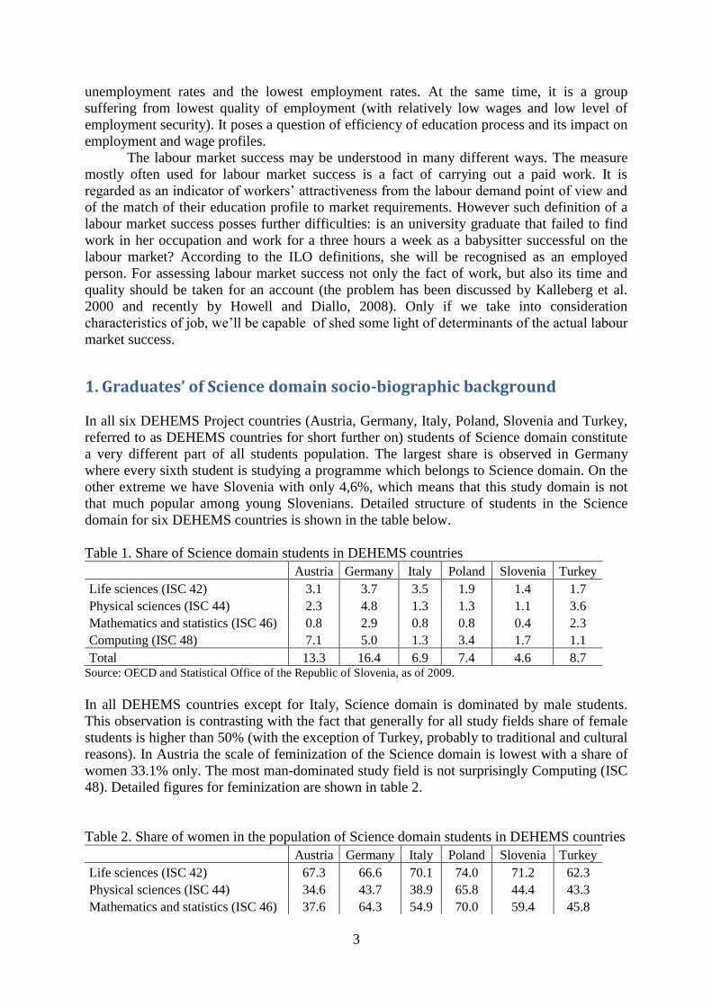
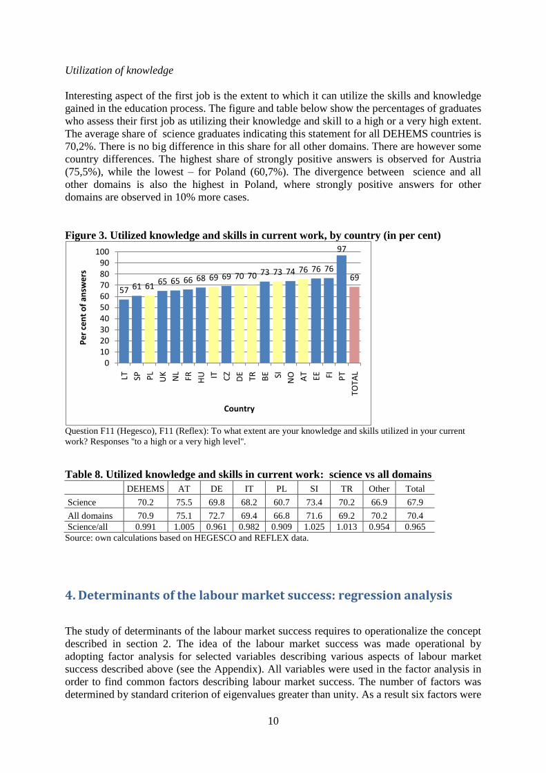
Utilization of knowledge

Interesting aspect of the first job is the extent to which it can utilize the skills and knowledge

gained in the education process. The figure and table below show the percentages of graduates

who assess their first job as utilizing their knowledge and skill to a high or a very high extent.

The average share of science graduates indicating this statement for all DEHEMS countries is

70,2%. There is no big difference in this share for all other domains. There are however some

country differences. The highest share of strongly positive answers is observed for Austria

(75,5%), while the lowest – for Poland (60,7%). The divergence between science and all

other domains is also the highest in Poland, where strongly positive answers for other

domains are observed in 10% more cases.

Figure 3. Utilized knowledge and skills in current work, by country (in per cent)

Question F11 (Hegesco), F11 (Reflex): To what extent are your knowledge and skills utilized in your current

work? Responses ''to a high or a very high level''.

Table 8. Utilized knowledge and skills in current work: science vs all domains


Science 70.2 75.5 69.8 68.2 60.7 73.4 70.2 66.9 67.9

All domains 70.9 75.1 72.7 69.4 66.8 71.6 69.2 70.2 70.4

Science/all 0.991 1.005 0.961 0.982 0.909 1.025 1.013 0.954 0.965


4. Determinants of the labour market success: regression analysis

The study of determinants of the labour market success requires to operationalize the concept

described in section 2. The idea of the labour market success was made operational by

adopting factor analysis for selected variables describing various aspects of labour market

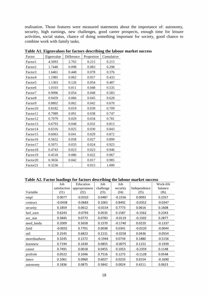
success described above (see the Appendix). All variables were used in the factor analysis in

order to find common factors describing labour market success. The number of factors was

determined by standard criterion of eigenvalues greater than unity. As a result six factors were

57 61 6165 65 66 68 69 69 70 70 73 73 74 76 76 76

97

69

0102030405060708090

100

LT SP PL

UK

NL

FR HU IT CZ

DE

TR BE SI

NO AT EE FI PT

TOTA

L

Pe

r ce

nt

of

answ

ers

Country

11

selected and named: job satisfaction, education appropriatness, job as a challenge, job

security, independence and work-life balance. Eigenvalues and factor loadings are presented

in the Appendix in the tables A1 and A2.

Determinants of six measures of labour market success were analysed using regression

method on a set of explanatory variables. The subset of significant regressors was chosen

using the stepwise selection method with 10% treshold significance level. Construction of

explanatory variables is presented in the Appendix in the table A3.

After merging data from those two data sets, an integrated dataset included 43311

observations for all REFLEX and HEGESCO countries. Dataset consisted of 533 variables, in

most cases of binary or discrete type. The most significant problems with the data elaboration

are listed below:

In many cases one particular piece of information is located in many variables,

each of which is relevant only for one country due to specific regulations. Average

grade is an example of this problem, with different grade systems in different

countries.

Estimating a domain-specific model for every country is hardly possible due to the

low number of observations in some domains (see tab. 3).

In case of some variables, the share of missing values is significant.

Basing on theoretical considerations, a list of potential dependant variables was

formulated that included almost thirty variables.

Data elaboration process included several steps. The first one consisted in processing

of each of the variables potentially useful for analysis. The “no answer” and “not relevant for

this country” etc. observations were treated as missing values and had been re-coded. In

several cases, where original variables seemed to contained too detailed information, new

variables were created as a result of an aggregation of several variable‟s values.

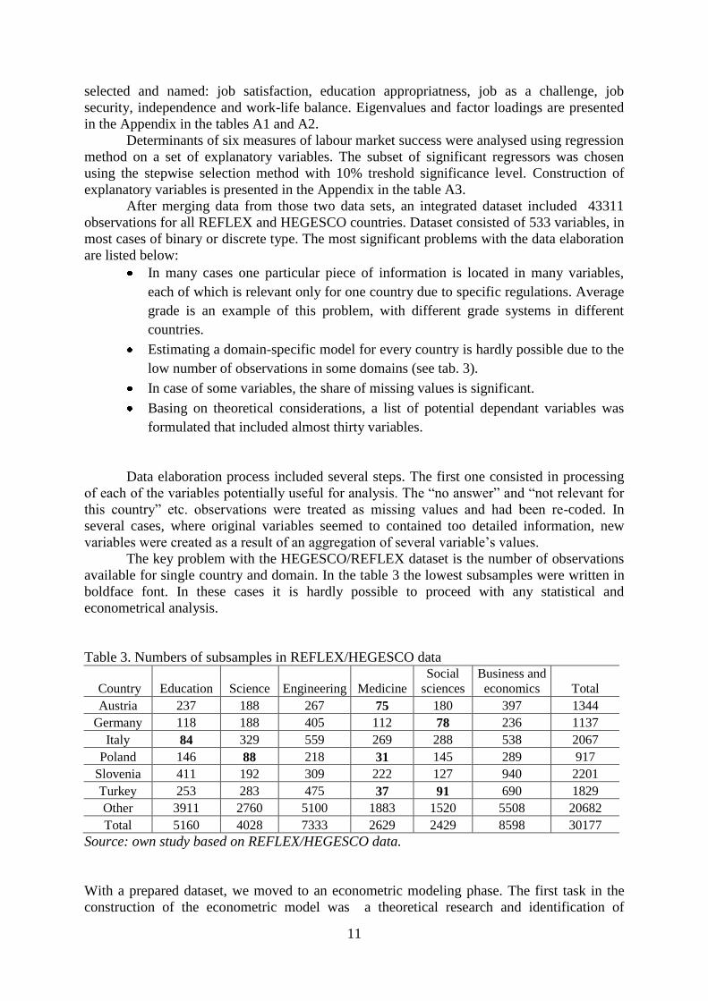
The key problem with the HEGESCO/REFLEX dataset is the number of observations

available for single country and domain. In the table 3 the lowest subsamples were written in

boldface font. In these cases it is hardly possible to proceed with any statistical and

econometrical analysis.

Table 3. Numbers of subsamples in REFLEX/HEGESCO data

Country Education Science Engineering Medicine Social

sciences Business and

economics Total

Austria 237 188 267 75 180 397 1344

Germany 118 188 405 112 78 236 1137

Italy 84 329 559 269 288 538 2067

Poland 146 88 218 31 145 289 917

Slovenia 411 192 309 222 127 940 2201

Turkey 253 283 475 37 91 690 1829

Other 3911 2760 5100 1883 1520 5508 20682

Total 5160 4028 7333 2629 2429 8598 30177

Source: own study based on REFLEX/HEGESCO data.

With a prepared dataset, we moved to an econometric modeling phase. The first task in the

construction of the econometric model was a theoretical research and identification of

12

dependent and explanatory variables. In the REFLEX/HEGESCO data set, experts were

able to identify almost sixty independent and almost thirty dependent variables. Preparation of

thirty separate econometric models for each domain would be too detailed and meaningless in

the context of the DEHEMS project‟s objectives. To resolve this problem Principal

Component Analysis3 was carried out.

The main objective of PCA is to reduce number of variables for analysis. This is done

by finding a relatively small number of components which are linear combinations of original

variables. PCA is based on analysis of correlations. The key idea is to group together

variables that behave similarly and transform the dataset from a large to a relatively small

number of variables by reducing dimensions. This process keeps as much information as

possible about the original data variability. Of course losing some information is a cost, but it

is compensated by increased readability and usefulness of the data. The number of factors

taken to further analysis is determined by the eigenvalues (if higher than one - total variance

is explained by a single component). Factor loadings describe the strength of input of

variables into components. Results of PCA are usually rotated so as each variable has high

loading in no more than one component. Analysis of factors gives a mathematical solution,

which is not always interpretable. Possible corrections to obtain sensible results and their

interpretation are done by a researcher. Components do not have direct numeric interpretation,

but they allow to identify variables of key significance for each of the factors.

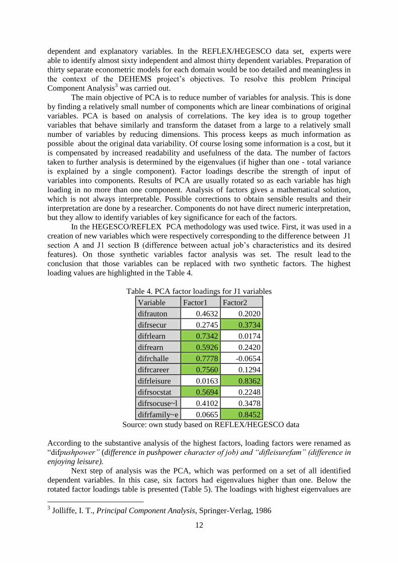
In the HEGESCO/REFLEX PCA methodology was used twice. First, it was used in a

creation of new variables which were respectively corresponding to the difference between J1

section A and J1 section B (difference between actual job‟s characteristics and its desired

features). On those synthetic variables factor analysis was set. The result lead to the

conclusion that those variables can be replaced with two synthetic factors. The highest

loading values are highlighted in the Table 4.

Table 4. PCA factor loadings for J1 variables

Variable Factor1 Factor2

difrauton 0.4632 0.2020

difrsecur 0.2745 0.3734

difrlearn 0.7342 0.0174

difrearn 0.5926 0.2420

difrchalle 0.7778 -0.0654

difrcareer 0.7560 0.1294

difrleisure 0.0163 0.8362

difrsocstat 0.5694 0.2248

difrsocuse~l 0.4102 0.3478

difrfamily~e 0.0665 0.8452

Source: own study based on REFLEX/HEGESCO data

According to the substantive analysis of the highest factors, loading factors were renamed as

“difpushpower” (difference in pushpower character of job) and “difleisurefam” (difference in

enjoying leisure).

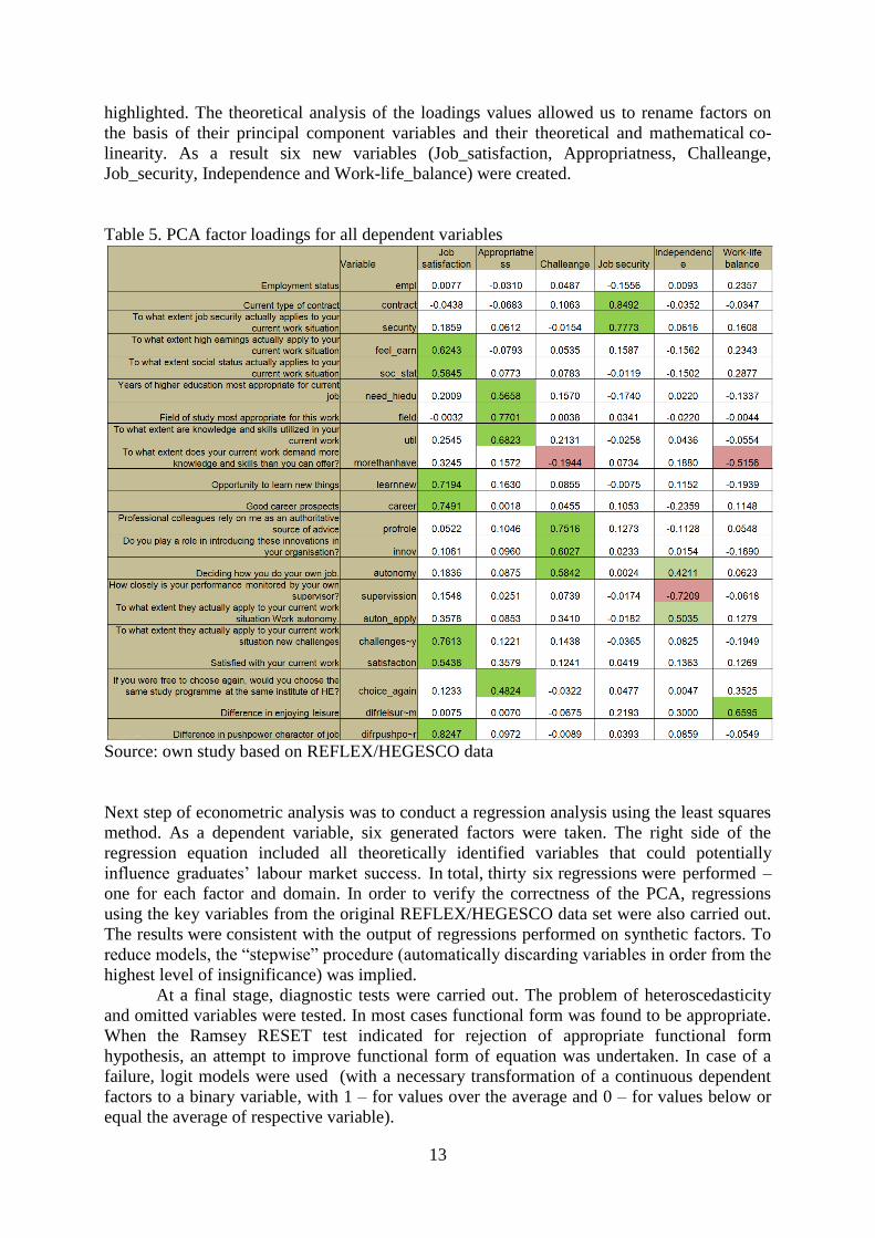
Next step of analysis was the PCA, which was performed on a set of all identified

dependent variables. In this case, six factors had eigenvalues higher than one. Below the

rotated factor loadings table is presented (Table 5). The loadings with highest eigenvalues are

3 Jolliffe, I. T., Principal Component Analysis, Springer-Verlag, 1986

13

highlighted. The theoretical analysis of the loadings values allowed us to rename factors on

the basis of their principal component variables and their theoretical and mathematical co-

linearity. As a result six new variables (Job_satisfaction, Appropriatness, Challeange,

Job_security, Independence and Work-life_balance) were created.

Table 5. PCA factor loadings for all dependent variables

Source: own study based on REFLEX/HEGESCO data

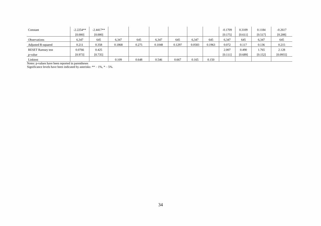
Next step of econometric analysis was to conduct a regression analysis using the least squares

method. As a dependent variable, six generated factors were taken. The right side of the

regression equation included all theoretically identified variables that could potentially

influence graduates‟ labour market success. In total, thirty six regressions were performed –

one for each factor and domain. In order to verify the correctness of the PCA, regressions

using the key variables from the original REFLEX/HEGESCO data set were also carried out.

The results were consistent with the output of regressions performed on synthetic factors. To

reduce models, the “stepwise” procedure (automatically discarding variables in order from the

highest level of insignificance) was implied.

At a final stage, diagnostic tests were carried out. The problem of heteroscedasticity

and omitted variables were tested. In most cases functional form was found to be appropriate.

When the Ramsey RESET test indicated for rejection of appropriate functional form

hypothesis, an attempt to improve functional form of equation was undertaken. In case of a

failure, logit models were used (with a necessary transformation of a continuous dependent

factors to a binary variable, with 1 – for values over the average and 0 – for values below or

equal the average of respective variable).

14

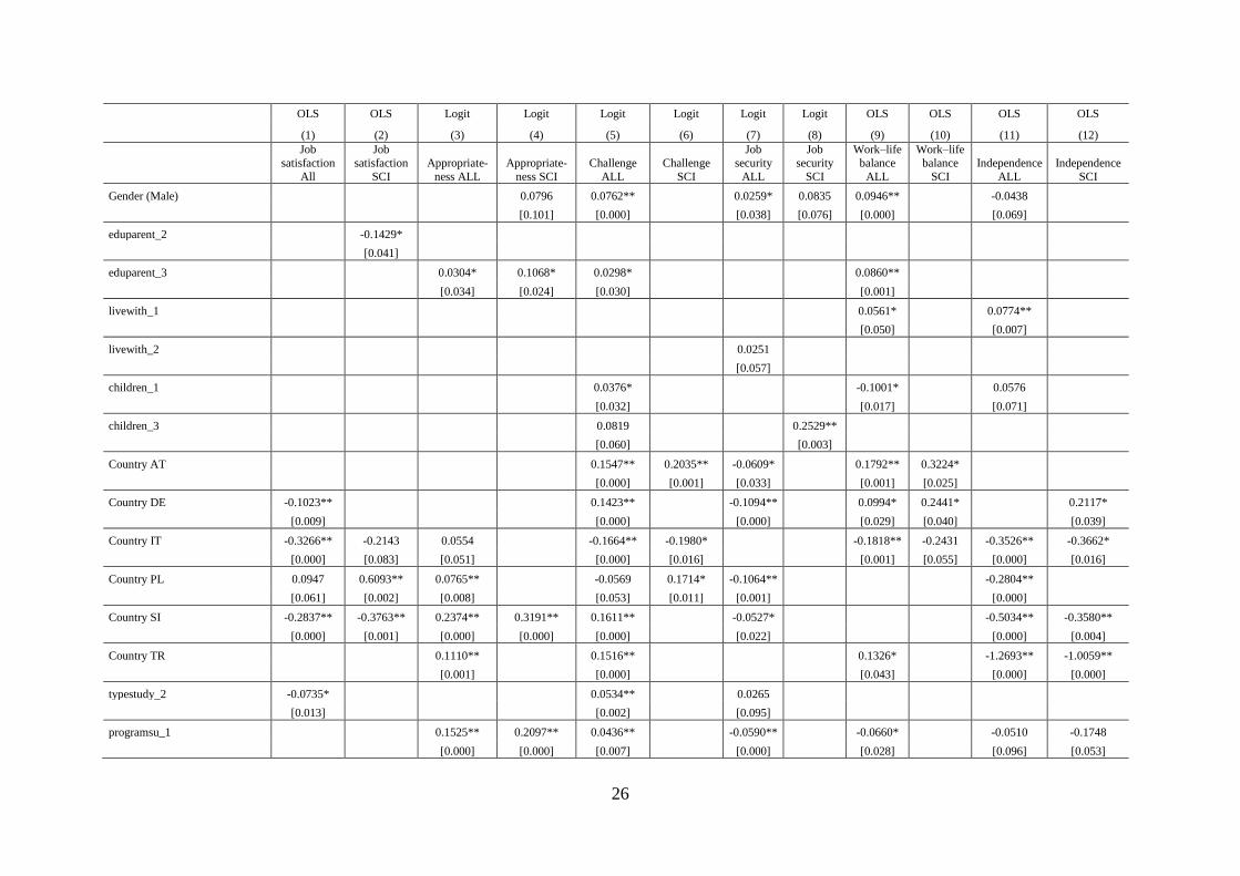
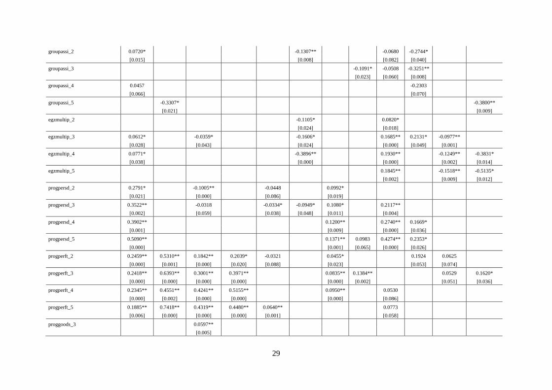
Detailed regression results are shown in the table A4 in the Appendix. Here, the most

interesting outcomes will be discussed and commented.

Socio-demographic characteristics

Gender was found a significant predictor of education appropriateness and job security only.

In both cases, male science graduates have higher values of those two variables than women.

Higher levels of parents education seems to decrease current job satisfaction while it increases

education appropriateness. It does not play any role for other dimensions of labour market

success. Country differences were found quite interesting. In terms of job satisfaction, Polish

science graduates have significantly higher values than European average, while Italian and

Slovenian graduates have significantly lower. In terms of education appropriateness, the only

country that is significantly different from European average is Slovenia, where graduates

have higher values of education appropriateness. Austrian and Polish science graduates

appear to have more challenging jobs than European average, while their Italian colleagues

have significantly lower values of this dimension. In terms of job security DEHEMS countries

do not differ from the European average. Austrian and German science graduates exhibit

higher values of work-life balance, while Italians are characterized by significantly lower

values. Italian, Slovenian and Turkish graduates (to the highest extent) are found to have

significantly lower work independence than the average. Austrian and Polish graduates do not

differ from the average significantly but Germans have significantly higher values of work

independence.

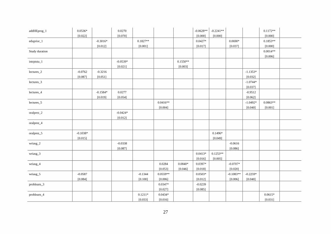
Study process characteristics

Completing master degree programme results in more education appropriateness but it

decreases work independence at the same time as compared to bachelor graduates. Having

finished additional HE programme reduces the probability of experiencing more job security.

Vocational secondary education background is correlated with lower values of overall job

satisfaction. Study duration was not found significant predictor of any of the labour market

success measures.

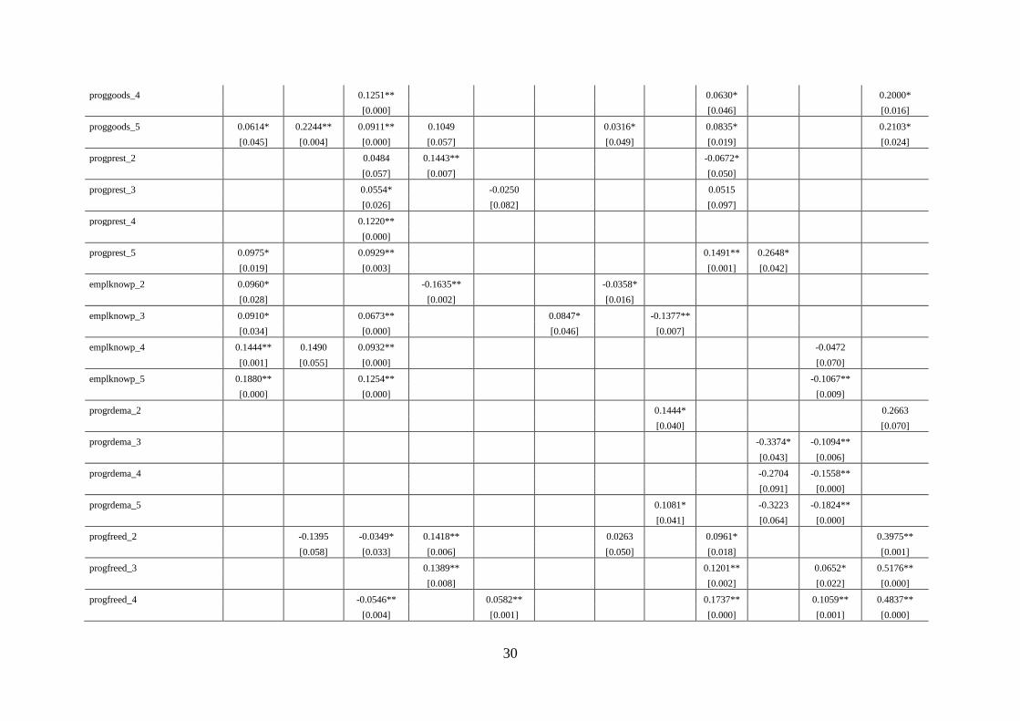
Programme characteristics

Graduates who evaluate their programmes as good for their personal development experience

higher values of job security and work-life balance. Those for whom the study programmes

were good for performing current job tasks exhibit higher current overall job satisfaction and

higher education appropriateness. The same is true about the programmes which were

regarded as good for starting work, but additionally graduates from such programmes

experience also higher work independence. Science graduates from prestigious programmes

experience higher work-life balance. Good knowledge of the programme by employers

influences positively the job satisfaction and has no relation to other labour market success

measures. Demanding programmes seem to reduce the work-life balance of science graduates.

High level of freedom in shaping own study programme increases education appropriateness.

Broad focus of the study programme decreases job satisfaction but increases work-life

balance. Vocational orientation of the programme also reduces job satisfaction but increases

job security.

15

Modes of teaching

From the set of variables describing modes of teaching, high extent of lectures decreases

current job satisfaction. High extent of oral presentations increases job security, while high

extent of written assignments reduces both education appropriateness and work-life balance.

High extent of problem based learning favours education appropriateness. Graduates who

stated that teacher was the main source of information experience higher job security. High

extent of theories and paradigms favours work independence but reduces education

appropriateness. High extent of research projects in the study programmes increases both job

satisfaction and job security while it decreases work independence. High extent of group

assignments influences job satisfaction and work independence negatively. And lastly, high

extent of multiple choice questions increases work-life balance but reduces challenge and

work independence.

Personal attitude

Science graduates with higher grades than average tend to have higher job security but lower

job challenge. Those who strived for highest possible marks experience lower overall job

satisfaction and lower work independence. Finally, those who performed extra work above

what was required to pass exams tend to have higher work independence than others.

International mobility

Spending time abroad during studies and after studies both for study and work purpose plays

very little role in determining labour market success. Graduates who spent time abroad after

graduation both for study and work purpose tend to have lower job security than others.

Higher values of work independence are observed for graduates who spent time abroad for

study purpose both during studies and after graduation.

Labour market experience

Study-related work experience acquired before HE tends to increase current job satisfaction

and work-life balance but reduces education appropriateness and work independence. Non

study-related work experience gained during HE increases current job satisfaction. Study-

related work experience during HE decreases job satisfaction but affects positively education

appropriateness and work challenge.

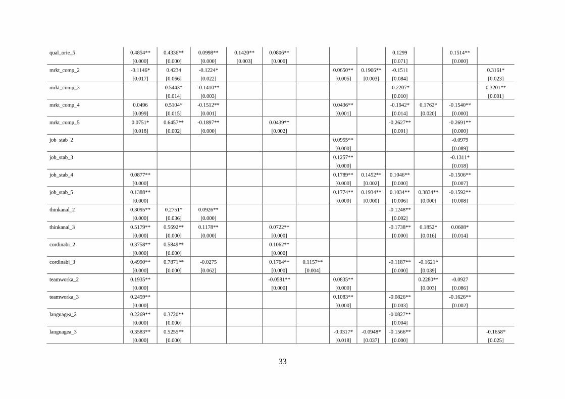
Firm or current job characteristics

Serious change that occurred in the firm increases job challenge. High extent of quality

orientation of firms increases job satisfaction and education appropriateness. More stable

demand on the market on which the firm operates results in higher job security and higher

work-life balance. High level of competence in analytical thinking, coordinating others‟ work

and language skills increase job satisfaction. The latter determinant reduces job security and

work independence.

16

5. Conclusions

In this article we tried to find determinants of the labour market success of science domain

graduates for six DEHEMS countries. The task is not trivial due to possible misunderstanding

of the term „success‟. Project results indicated that labour market success should be

understood in terms of the following aspects: employment status, type of contract, job

security, job autonomy, earnings, social status, appropriateness of education, utilization of

knowledge, opportunity to learn new things, career prospects, professional role, new

challengesm , work satisfaction. In order to reduce the number of dependent variables of the

study we conducted a PCA analysis and found 6 factors, which were then used as measures of

labour market success. The set of determinants included variables describing socio-

demographic characteristics, study process characteristics, programme characteristics, modes

of teaching and learning, personal attitude, international mobility, labour market experience,

firm or current job characteristics. In the process of econometric procedure robust OLS

estimations were conducted, and where necessary (rejection of the null hypothesis of correct

functional form) logistic regressions were applied.

Regression analysis revealed a number of interesting facts. In some cases labour

market success can be related to parents education. Therefore one can argue that investment in

HE can be seen to have some cross-generational positive social external effects. Country

dummies were found to be significant in many cases, so one can only regret that insufficient

number of observations did not allow for more detailed study of country specifics. Study

process characteristics seemed to play relatively minor role in determining future labour

market success. On the other hand the most important factors come from the set of variables

describing programme characteristics and modes of teaching but also firm or current job

characteristics. It is worth noting that study programme characteristics and modes of teaching

are under control of HE management. Regression results indicate that programmes regarded

as good for performing current job tasks, regarded as good basis for starting work, known by

employers favour labour market success in terms of overall job satisfaction, which is a

mixture of high earnings, social status, good career prospects and job matching expectations.

Further studies could be conducted to look for other aspects of labour market success.

For instance, it would be very interesting to look at qualification mismatch and the problem of

under or over qualification of young labour force. Dynamic analyses using panel data could

also shed some light on the problem of unemployment persistence, employment stability and

labour market flows for the graduates across Europe.

17

6. Appendix

Variables identified as components of the labour market success:

Employment status (empl) – 1: working, 0: not working;

Type of contract (contract) – 0: fixed term, 1: self-employed, 2: full time contract;

Job security (security) – to what extent job security applies to current work – 1 (not at all) to 5

(to a very high extent);

Job autonomy (auton_apply) – to what extent job autonomy applies to current work – 1 (not

at all) to 5 (to a very high extent);

Earnings (feel_earn) – to what extent high earnings apply to current work – 1 (not at all) to 5

(to a very high extent);

Social status (soc_stat) – to what extent social status applies to current work – 1 (not at all) to

5 (to a very high extent);

Years of higher education most appropriate for current job (need_hiedu);

Field of study most appropriate for this work (field) – 0: completely different than possessed,

1: own or related;

Utilization of knowledge (util) – to what extent are knowledge and skills utilized in current

work – 1 (not at all) to 5 (to a very high extent);

Demand for more skills (morethanhave) – to what extent does current work demand more

knowledge and skills than can actually be offered – 1 (not at all) to 5 (to a very high extent);

Opportunity to learn new things (learnnew) – to what extent opportunity to learn new things

applies to current work – 1 (not at all) to 5 (to a very high extent);

Good career prospects (career) – to what extent good career prospects applies to current work

– 1 (not at all) to 5 (to a very high extent);

Professional role (profrole) – professional colleagues rely on me as an authoritative source of

advice: 1 (not at all) to 5 (to a very high extent);

Innovativeness (innov) – playing a role in introducing innovations in organisation (Product or

service, Technology, tools or instruments, knowledge or methods);

Own deciding (autonomy) – to what extent are you responsible for deciding how you do your

own job – 1 (not at all) to 5 (to a very high extent);

Supervission (supervission) – how closely is performance monitored by own supervisor – 1

(not very closely) to 5 (very closely);

New challenges (challenges_apply) – to what extent new challegnes apply to current work – 1

(not at all) to 5 (to a very high extent);

Work satisfaction (satisfaction) – how satisfied are you with your current work – 1 (very

dissatisfied) to 5 (very satisfied);

Choosing the same programme again (choice) – would you choose the same study programme

at the same institute – 1: Yes, 2: No, a different study programme at the same institute, 3: No,

the same study programme at a different institute, 4: No, a different study programme at a

different institute, 5: No, I would decide not to study at all;

difrleisurefam - divergence between own valuation and the actual realisation of work features

related to leisure time and combining work and family duties;

difrpushpower - divergence between own valuation and the actual realisation of work features

related to earnings, career prospects, social status, going something important for society, new

challenges.

The last two variables were created using scoring coefficinets after factor analysis on

measures of the divergence between the importance of given job feature and its actual

18

realisation. Those features were measured statements about the importance of: autonomy,

security, high earnings, new challenges, good career prospects, enough time for leisure

activities, social status, chance of doing something important for society, good chance to

combine work with family tasks.

Table A1. Eigenvalues for factors describing the labour market success

Factor Eigenvalue Difference Proportion Cumulative

Factor1 4.5093 2.765 0.215 0.215

Factor2 1.7440 0.098 0.083 0.298

Factor3 1.6461 0.448 0.078 0.376

Factor4 1.1985 0.062 0.057 0.433

Factor5 1.1363 0.126 0.054 0.487

Factor6 1.0103 0.011 0.048 0.535

Factor7 0.9996 0.054 0.048 0.583

Factor8 0.9459 0.066 0.045 0.628

Factor9 0.8802 0.062 0.042 0.670

Factor10 0.8182 0.019 0.039 0.709

Factor11 0.7989 0.091 0.038 0.747

Factor12 0.7079 0.029 0.034 0.781

Factor13 0.6793 0.048 0.032 0.813

Factor14 0.6316 0.025 0.030 0.843

Factor15 0.6063 0.041 0.029 0.872

Factor16 0.5652 0.058 0.027 0.899

Factor17 0.5071 0.033 0.024 0.923

Factor18 0.4743 0.023 0.023 0.946

Factor19 0.4518 0.086 0.022 0.967

Factor20 0.3656 0.042 0.017 0.985

Factor21 0.3236 . 0.015 1.000

Table A2. Factor loadings for factors describing the labour market success

Variable

Job

satisfaction

(f1)

Education

appropriatness

(f2)

Job

challenge

(f3)

Job

security

(f4)

Independence

(f5)

Work-life

balance

(f6)

empl 0.0077 -0.0310 0.0487 -0.1556 0.0093 0.2357

contract -0.0438 -0.0683 0.1063 0.8492 -0.0352 -0.0347

security 0.1859 0.0612 -0.0154 0.7773 0.0616 0.1608

feel_earn 0.6243 -0.0793 0.0535 0.1587 -0.1562 0.2343

soc_stat 0.5845 0.0773 0.0783 -0.0119 -0.1502 0.2877

need_hiedu 0.2009 0.5658 0.1570 -0.1740 0.0220 -0.1337

field -0.0032 0.7701 0.0038 0.0341 -0.0220 -0.0044

util 0.2545 0.6823 0.2131 -0.0258 0.0436 -0.0554

morethanhave 0.3245 0.1572 -0.1944 0.0734 0.1880 -0.5156

learnnew 0.7194 0.1630 0.0855 -0.0075 0.1152 -0.1939

career 0.7491 0.0018 0.0455 0.1053 -0.2359 0.1148

profrole 0.0522 0.1046 0.7516 0.1273 -0.1128 0.0548

innov 0.1061 0.0960 0.6027 0.0233 0.0154 -0.1690

autonomy 0.1836 0.0875 0.5842 0.0024 0.4211 0.0623

19

supervission 0.1548 0.0251 0.0739 -0.0174 -0.7209 -0.0618

auton_apply 0.3578 0.0853 0.3410 -0.0182 0.5035 0.1279

challenges_apply 0.7613 0.1221 0.1438 -0.0365 0.0825 -0.1949

satisfaction 0.5438 0.3579 0.1241 0.0419 0.1363 0.1269

choice 0.1233 0.4824 -0.0322 0.0477 0.0047 0.3525

difrleisurefam 0.0075 0.0070 -0.0675 0.2193 0.3000 0.6595

difrpushpower 0.8247 0.0972 -0.0089 0.0393 0.0859 -0.0549

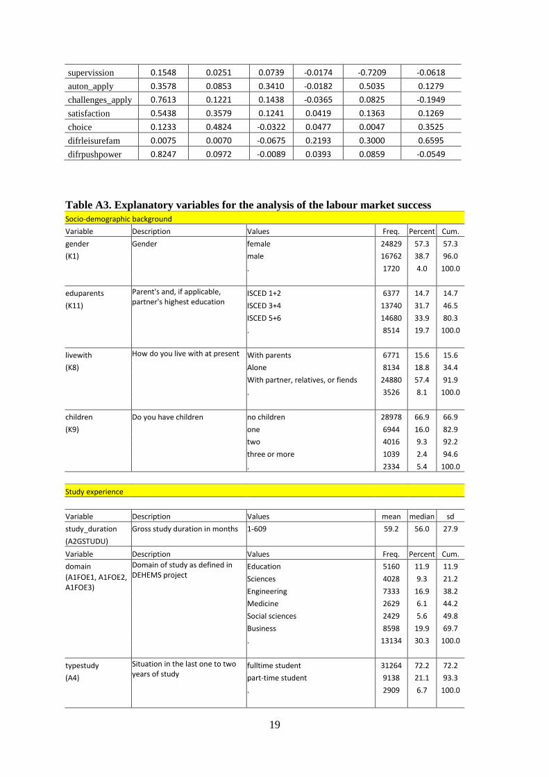
Table A3. Explanatory variables for the analysis of the labour market success

Socio-demographic background

Variable Description Values Freq. Percent Cum.

gender Gender female 24829 57.3 57.3

(K1)

male 16762 38.7 96.0

. 1720 4.0 100.0

eduparents Parent's and, if applicable,

partner's highest education ISCED 1+2 6377 14.7 14.7

(K11) ISCED 3+4 13740 31.7 46.5

ISCED 5+6 14680 33.9 80.3

. 8514 19.7 100.0

livewith How do you live with at present With parents 6771 15.6 15.6

(K8) Alone 8134 18.8 34.4

With partner, relatives, or fiends 24880 57.4 91.9

. 3526 8.1 100.0

children Do you have children no children 28978 66.9 66.9

(K9)

one 6944 16.0 82.9

two 4016 9.3 92.2

three or more 1039 2.4 94.6

. 2334 5.4 100.0

Study experience

Variable Description Values mean median sd

study_duration Gross study duration in months 1-609 59.2 56.0 27.9

(A2GSTUDU) Variable Description Values Freq. Percent Cum.

domain Domain of study as defined in DEHEMS project

Education 5160 11.9 11.9

(A1FOE1, A1FOE2, A1FOE3)

Sciences 4028 9.3 21.2

Engineering 7333 16.9 38.2

Medicine 2629 6.1 44.2

Social sciences 2429 5.6 49.8

Business 8598 19.9 69.7

. 13134 30.3 100.0

typestudy Situation in the last one to two

years of study fulltime student 31264 72.2 72.2

(A4) part-time student 9138 21.1 93.3

. 2909 6.7 100.0

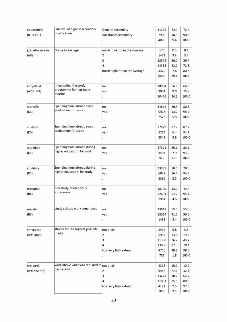
20

edupriorHE Sublevel of highest secondary qualification

General secondary 31334 72.4 72.4

(B1LEVEL) Vocational secondary 7909 18.3 90.6

. 4068 9.4 100.0

gradetoaverage Grade to average much lower than the average 173 0.4 0.4

(A3) 2 1422 3.3 3.7

3 15578 36.0 39.7

4 14368 33.2 72.8

much higher than the average 3370 7.8 80.6

. 8400 19.4 100.0

intrptstud Interrupting the study

programme for 4 or more months

no 28934 66.8 66.8

(A2IRUPT) yes 3901 9.0 75.8

. 10476 24.2 100.0

workafts Spending time abroad since

graduation: for work no 34862 80.5 80.5

(K6) yes 5923 13.7 94.2

. 2526 5.8 100.0

studafts Spending time abroad since

graduation: for study no 37979 87.7 87.7

(K6) yes 2784 6.4 94.1

. 2548 5.9 100.0

workdurs Spending time abroad during

higher education: for work no 37271 86.1 86.1

(K5) yes 3404 7.9 93.9

. 2636 6.1 100.0

studdurs Spending time abroad during

higher education: for study no 33989 78.5 78.5

(K5) yes 6927 16.0 94.5

. 2395 5.5 100.0

nrexpdur non study-related work

experience no 18729 43.2 43.2

(B4) yes 22601 52.2 95.4

. 1981 4.6 100.0

rexpdur study-related work experience no 23819 55.0 55.0

(B3) yes 18024 41.6 96.6

. 1468 3.4 100.0

strivebest strived for the highest possible

marks not at all 2494 5.8 5.8

(A9STRIVE) 2 5957 13.8 19.5

3 11358 26.2 45.7

4 13996 32.3 78.1

to a very high extent 8750 20.2 98.3

. 756 1.8 100.0

extrwork work above what was required to

pass exams not at all 4318 10.0 10.0

(A9EXWORK) 2 9582 22.1 32.1

3 13273 30.7 62.7

4 11061 25.5 88.3


. 956 2.2 100.0

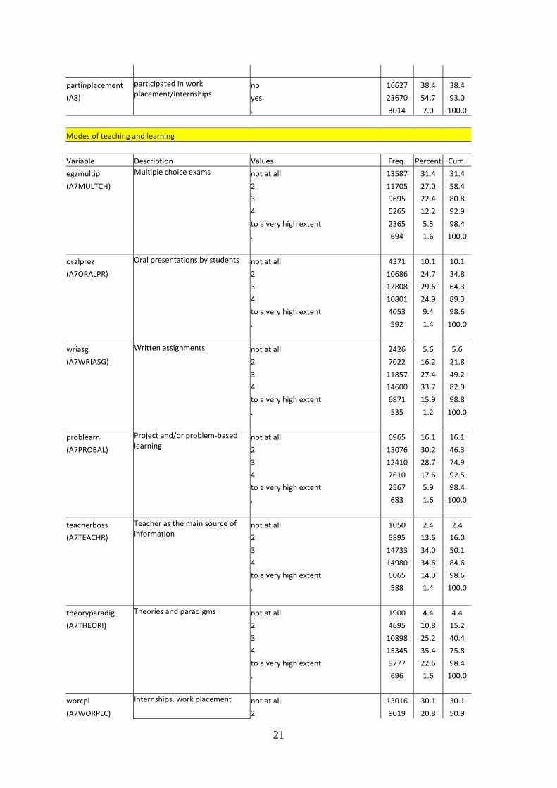
21

partinplacement participated in work

placement/internships no 16627 38.4 38.4

(A8) yes 23670 54.7 93.0

. 3014 7.0 100.0

Modes of teaching and learning


egzmultip Multiple choice exams not at all 13587 31.4 31.4

(A7MULTCH) 2 11705 27.0 58.4

3 9695 22.4 80.8

4 5265 12.2 92.9


. 694 1.6 100.0

oralprez Oral presentations by students not at all 4371 10.1 10.1

(A7ORALPR) 2 10686 24.7 34.8

3 12808 29.6 64.3

4 10801 24.9 89.3


. 592 1.4 100.0

wriasg Written assignments not at all 2426 5.6 5.6

(A7WRIASG) 2 7022 16.2 21.8

3 11857 27.4 49.2

4 14600 33.7 82.9


. 535 1.2 100.0

problearn Project and/or problem-based

learning not at all 6965 16.1 16.1

(A7PROBAL) 2 13076 30.2 46.3

3 12410 28.7 74.9

4 7610 17.6 92.5


. 683 1.6 100.0

teacherboss Teacher as the main source of

information not at all 1050 2.4 2.4

(A7TEACHR) 2 5895 13.6 16.0

3 14733 34.0 50.1

4 14980 34.6 84.6


. 588 1.4 100.0

theoryparadig Theories and paradigms not at all 1900 4.4 4.4

(A7THEORI) 2 4695 10.8 15.2

3 10898 25.2 40.4

4 15345 35.4 75.8


. 696 1.6 100.0

worcpl Internships, work placement not at all 13016 30.1 30.1

(A7WORPLC) 2 9019 20.8 50.9

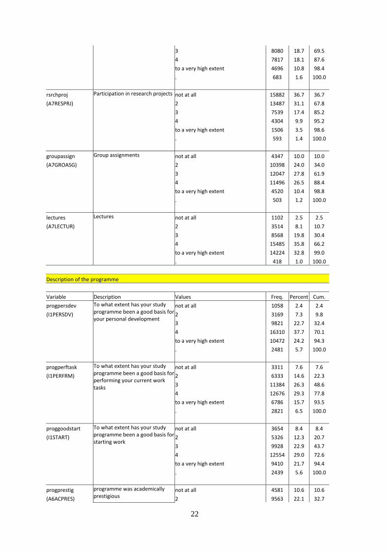
22

3 8080 18.7 69.5

4 7817 18.1 87.6


. 683 1.6 100.0

rsrchproj Participation in research projects not at all 15882 36.7 36.7

(A7RESPRJ) 2 13487 31.1 67.8

3 7539 17.4 85.2

4 4304 9.9 95.2


. 593 1.4 100.0

groupassign Group assignments not at all 4347 10.0 10.0

(A7GROASG) 2 10398 24.0 34.0

3 12047 27.8 61.9

4 11496 26.5 88.4


. 503 1.2 100.0

lectures Lectures not at all 1102 2.5 2.5

(A7LECTUR) 2 3514 8.1 10.7

3 8568 19.8 30.4

4 15485 35.8 66.2


. 418 1.0 100.0

Description of the programme


progpersdev To what extent has your study programme been a good basis for your personal development

not at all 1058 2.4 2.4

(I1PERSDV) 2 3169 7.3 9.8

3 9821 22.7 32.4

4 16310 37.7 70.1


. 2481 5.7 100.0

progperftask To what extent has your study

programme been a good basis for performing your current work tasks

not at all 3311 7.6 7.6

(I1PERFRM) 2 6333 14.6 22.3

3 11384 26.3 48.6

4 12676 29.3 77.8


. 2821 6.5 100.0

proggoodstart To what extent has your study

programme been a good basis for starting work

not at all 3654 8.4 8.4

(I1START) 2 5326 12.3 20.7

3 9928 22.9 43.7

4 12554 29.0 72.6


. 2439 5.6 100.0

progprestig programme was academically

prestigious not at all 4581 10.6 10.6

(A6ACPRES) 2 9563 22.1 32.7

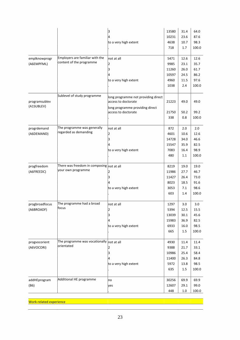
23

3 13580 31.4 64.0

4 10231 23.6 87.6


. 718 1.7 100.0

emplknowprogr Employers are familiar with the

content of the programme not at all 5471 12.6 12.6

(A6EMPFML) 2 9985 23.1 35.7

3 11260 26.0 61.7

4 10597 24.5 86.2


. 1038 2.4 100.0

programsublev

Sublevel of study programme long programme not providing direct access to doctorate 21223 49.0 49.0

(A1SUBLEV) long programme providing direct access to doctorate 21750 50.2 99.2

. 338 0.8 100.0

progrdemand The programme was generally

regarded as demanding not at all 872 2.0 2.0

(A6DEMAND) 2 4601 10.6 12.6

3 14728 34.0 46.6

4 15547 35.9 82.5


. 480 1.1 100.0

progfreedom There was freedom in composing

your own programme not at all 8219 19.0 19.0

(A6FREEDC) 2 11986 27.7 46.7

3 11427 26.4 73.0

4 8023 18.5 91.6


. 603 1.4 100.0

progbroadfocus The programme had a broad

focus not at all 1297 3.0 3.0

(A6BROADF) 2 5394 12.5 15.5

3 13039 30.1 45.6

4 15983 36.9 82.5


. 665 1.5 100.0

progvocorient The programme was vocationally

orientated not at all 4930 11.4 11.4

(A6VOCORI) 2 9388 21.7 33.1

3 10986 25.4 58.4

4 11400 26.3 84.8


. 635 1.5 100.0

addHEprogram Additional HE programme no 30256 69.9 69.9

(B6) yes 12607 29.1 99.0

. 448 1.0 100.0

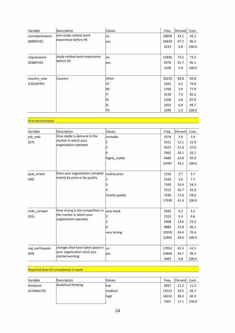
Work-related experience

24


nonrelpriorwork non study-related work experience before HE

no 18658 43.1 43.1

(B4BEFHE) yes 20430 47.2 90.3

. 4223 9.8 100.0

relpriorwork study-related work experience

before HE no 31826 73.5 73.5

(B3BEFHE) yes 9379 21.7 95.1

. 2106 4.9 100.0

country_new Country Other 30229 69.8 69.8

(COUNTRY)

AT 1821 4.2 74.0

DE 1700 3.9 77.9

IT 3139 7.3 85.2

PL 1200 2.8 87.9

SI 2923 6.8 94.7

TR 2299 5.3 100.0

Firm environment


job_stab How stable is demand in the market in which your organization operates

unstable 1674 3.9 3.9

(G7) 2 5221 12.1 15.9

3 9107 21.0 37.0

4 7842 18.1 55.1

highly_stable 4680 10.8 65.9

. 14787 34.1 100.0

qual_orient Does your organization compete

mainly by price or by quality mailny price 1163 2.7 2.7

(G6) 2 2164 5.0 7.7

3 7200 16.6 24.3

4 7215 16.7 41.0

mainly quality 7630 17.6 58.6

. 17939 41.4 100.0

mrkt_compet How strong is the competition in

the market in which your organization operates

very week 1832 4.2 4.2

(G5) 2 2323 5.4 9.6

3 5908 13.6 23.2

4 9884 22.8 46.1

very strong 10559 24.4 70.4

. 12805 29.6 100.0

org_earthquake changes that have taken place in

your organization since you started working

no 17952 41.5 41.5

(G9) yes 23694 54.7 96.2

. 1665 3.8 100.0

Required level of competence in work


thinkanal Analytical thinking low 4837 11.2 11.2

(H1ANALYR) medium 14515 33.5 44.7

high 16552 38.2 82.9

. 7407 17.1 100.0

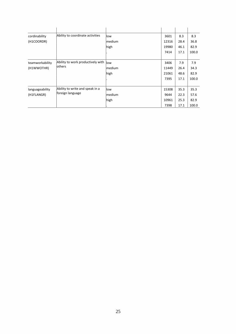
25

cordinability Ability to coordinate activities low 3601 8.3 8.3

(H1COORDR) medium 12316 28.4 36.8

high 19980 46.1 82.9

. 7414 17.1 100.0

teamworkability Ability to work productively with

others low 3406 7.9 7.9

(H1WWOTHR) medium 11449 26.4 34.3

high 21061 48.6 82.9

. 7395 17.1 100.0

languageability Ability to write and speak in a

foreign language low 15308 35.3 35.3

(H1FLANGR) medium 9644 22.3 57.6

high 10961 25.3 82.9

. 7398 17.1 100.0

26

OLS OLS Logit Logit Logit Logit Logit Logit OLS OLS OLS OLS

(1) (2) (3) (4) (5) (6) (7) (8) (9) (10) (11) (12)

Job

satisfaction

All

Job

satisfaction

SCI

Appropriate-

ness ALL

Appropriate-

ness SCI

Challenge

ALL

Challenge

SCI

Job

security

ALL

Job

security

SCI

Work–life

balance

ALL

Work–life

balance

SCI

Independence

ALL

Independence

SCI

Gender (Male) 0.0796 0.0762** 0.0259* 0.0835 0.0946** -0.0438

[0.101] [0.000] [0.038] [0.076] [0.000] [0.069]

eduparent_2 -0.1429*

[0.041]

eduparent_3 0.0304* 0.1068* 0.0298* 0.0860**

[0.034] [0.024] [0.030] [0.001]

livewith_1 0.0561* 0.0774**

[0.050] [0.007]

livewith_2 0.0251

[0.057]

children_1 0.0376* -0.1001* 0.0576

[0.032] [0.017] [0.071]

children_3 0.0819 0.2529**

[0.060] [0.003]

Country AT 0.1547** 0.2035** -0.0609* 0.1792** 0.3224*

[0.000] [0.001] [0.033] [0.001] [0.025]

Country DE -0.1023** 0.1423** -0.1094** 0.0994* 0.2441* 0.2117*

[0.009] [0.000] [0.000] [0.029] [0.040] [0.039]

Country IT -0.3266** -0.2143 0.0554 -0.1664** -0.1980* -0.1818** -0.2431 -0.3526** -0.3662*

[0.000] [0.083] [0.051] [0.000] [0.016] [0.001] [0.055] [0.000] [0.016]

Country PL 0.0947 0.6093** 0.0765** -0.0569 0.1714* -0.1064** -0.2804**

[0.061] [0.002] [0.008] [0.053] [0.011] [0.001] [0.000]

Country SI -0.2837** -0.3763** 0.2374** 0.3191** 0.1611** -0.0527* -0.5034** -0.3580**

[0.000] [0.001] [0.000] [0.000] [0.000] [0.022] [0.000] [0.004]

Country TR 0.1110** 0.1516** 0.1326* -1.2693** -1.0059**

[0.001] [0.000] [0.043] [0.000] [0.000]

typestudy_2 -0.0735* 0.0534** 0.0265

[0.013] [0.002] [0.095]

programsu_1 0.1525** 0.2097** 0.0436** -0.0590** -0.0660* -0.0510 -0.1748

[0.000] [0.000] [0.007] [0.000] [0.028] [0.096] [0.053]

27

addHEprog_1 0.0536* 0.0270 -0.0628** -0.2241** 0.1172**

[0.022] [0.070] [0.000] [0.000] [0.000]

eduprior_1 -0.3016* 0.1827** 0.0427* 0.0690* 0.1853**

[0.012] [0.001] [0.017] [0.037] [0.000]

Study duration 0.0014**

[0.006]

intrptstu_1 -0.0539* 0.1550**

[0.021] [0.003]

lectures_2 -0.0762 -0.3216 -1.1353*

[0.087] [0.051] [0.032]

lectures_3 -1.0744*

[0.037]

lectures_4 -0.1584* 0.0277 -0.9512

[0.019] [0.054] [0.062]

lectures_5 0.0416** -1.0492* 0.0863**

[0.004] [0.040] [0.001]

oralprez_2 -0.0424*

[0.012]

oralprez_4

oralprez_5 -0.1038* 0.1496*

[0.015] [0.049]

wriasg_2 -0.0338 -0.0616

[0.087] [0.086]

wriasg_3 0.0413* 0.1253**

[0.016] [0.005]

wriasg_4 0.0284 0.0840* 0.0397* -0.0707*

[0.053] [0.046] [0.018] [0.020]

wriasg_5 -0.0587 -0.1344 0.0559** 0.0503* -0.1083** -0.2259*

[0.084] [0.100] [0.006] [0.012] [0.006] [0.040]

problearn_3 0.0347* -0.0239

[0.027] [0.085]

problearn_4 0.1211* 0.0434* 0.0615*

[0.033] [0.016] [0.031]

28

problearn_5

teacherbo_2 0.1439** 0.0714

[0.001] [0.057]

teacherbo_3 0.1094* 0.0688 0.1380*

[0.015] [0.073] [0.014]

teacherbo_4 0.1130* 0.1009** 0.1870** -0.0525*

[0.012] [0.007] [0.001] [0.030]

teacherbo_5 0.1297** 0.0757* 0.1659**

[0.003] [0.045] [0.007]

theorypar_2 -0.0746 0.4729*

[0.069] [0.020]

theorypar_3 0.0860** -0.0664 -0.1725** 0.3774*

[0.002] [0.086] [0.001] [0.042]

theorypar_4 0.0621* -0.0933* -0.0838 0.3629*

[0.020] [0.015] [0.090] [0.049]

theorypar_5 -0.1160** -0.0844* 0.4069*

[0.006] [0.021] [0.036]

worcpl_2 0.0901

[0.053]

worcpl_3 -0.0284 0.1361**

[0.095] [0.007]

worcpl_4 -0.0529

[0.075]

worcpl_5 0.0953** -0.1624 0.0953* 0.4404**

[0.000] [0.102] [0.016] [0.003]

rsrchproj_2 -0.0774**

[0.007]

rsrchproj_3 -0.0320 0.0322 0.1125* -0.1024**

[0.085] [0.060] [0.020] [0.002]

rsrchproj_4 -0.0399 0.0456* -0.0440* -0.1264** -0.2134*

[0.093] [0.034] [0.029] [0.002] [0.049]

rsrchproj_5 0.2289** 0.3079* -0.0934* 0.0852*

[0.001] [0.049] [0.040] [0.025]

29

groupassi_2 0.0720* -0.1307** -0.0680 -0.2744*

[0.015] [0.008] [0.082] [0.040]

groupassi_3 -0.1091* -0.0508 -0.3251**

[0.023] [0.060] [0.008]

groupassi_4 0.0457 -0.2303

[0.066] [0.070]

groupassi_5 -0.3307* -0.3800**

[0.021] [0.009]

egzmultip_2 -0.1105* 0.0820*

[0.024] [0.018]

egzmultip_3 0.0612* -0.0359* -0.1606* 0.1685** 0.2131* -0.0977**

[0.028] [0.043] [0.024] [0.000] [0.049] [0.001]

egzmultip_4 0.0771* -0.3896** 0.1930** -0.1249** -0.3831*

[0.038] [0.000] [0.000] [0.002] [0.014]

egzmultip_5 0.1845** -0.1518** -0.5135*

[0.002] [0.009] [0.012]

progpersd_2 0.2791* -0.1005** -0.0448 0.0992*

[0.021] [0.000] [0.086] [0.019]

progpersd_3 0.3522** -0.0318 -0.0334* -0.0949* 0.1080* 0.2117**

[0.002] [0.059] [0.038] [0.048] [0.011] [0.004]

progpersd_4 0.3902** 0.1200** 0.2740** 0.1669*

[0.001] [0.009] [0.000] [0.036]

progpersd_5 0.5090** 0.1371** 0.0983 0.4274** 0.2353*

[0.000] [0.001] [0.065] [0.000] [0.026]

progperft_2 0.2459** 0.5310** 0.1842** 0.2039* -0.0321 0.0455* 0.1924 0.0625

[0.000] [0.001] [0.000] [0.020] [0.088] [0.023] [0.053] [0.074]

progperft_3 0.2418** 0.6393** 0.3001** 0.3971** 0.0835** 0.1384** 0.0529 0.1620*

[0.000] [0.000] [0.000] [0.000] [0.000] [0.002] [0.051] [0.036]

progperft_4 0.2345** 0.4551** 0.4241** 0.5155** 0.0950** 0.0530

[0.000] [0.002] [0.000] [0.000] [0.000] [0.086]

progperft_5 0.1885** 0.7418** 0.4319** 0.4480** 0.0640** 0.0773

[0.006] [0.000] [0.000] [0.000] [0.001] [0.058]

proggoods_3 0.0597**

[0.005]

30

proggoods_4 0.1251** 0.0630* 0.2000*

[0.000] [0.046] [0.016]

proggoods_5 0.0614* 0.2244** 0.0911** 0.1049 0.0316* 0.0835* 0.2103*

[0.045] [0.004] [0.000] [0.057] [0.049] [0.019] [0.024]

progprest_2 0.0484 0.1443** -0.0672*

[0.057] [0.007] [0.050]

progprest_3 0.0554* -0.0250 0.0515

[0.026] [0.082] [0.097]

progprest_4 0.1220**

[0.000]

progprest_5 0.0975* 0.0929** 0.1491** 0.2648*

[0.019] [0.003] [0.001] [0.042]

emplknowp_2 0.0960* -0.1635** -0.0358*

[0.028] [0.002] [0.016]

emplknowp_3 0.0910* 0.0673** 0.0847* -0.1377**

[0.034] [0.000] [0.046] [0.007]

emplknowp_4 0.1444** 0.1490 0.0932** -0.0472

[0.001] [0.055] [0.000] [0.070]

emplknowp_5 0.1880** 0.1254** -0.1067**

[0.000] [0.000] [0.009]

progrdema_2 0.1444* 0.2663

[0.040] [0.070]

progrdema_3 -0.3374* -0.1094**

[0.043] [0.006]

progrdema_4 -0.2704 -0.1558**

[0.091] [0.000]

progrdema_5 0.1081* -0.3223 -0.1824**

[0.041] [0.064] [0.000]

progfreed_2 -0.1395 -0.0349* 0.1418** 0.0263 0.0961* 0.3975**

[0.058] [0.033] [0.006] [0.050] [0.018] [0.001]

progfreed_3 0.1389** 0.1201** 0.0652* 0.5176**

[0.008] [0.002] [0.022] [0.000]

progfreed_4 -0.0546** 0.0582** 0.1737** 0.1059** 0.4837**

[0.004] [0.001] [0.000] [0.001] [0.000]

31

progfreed_5 0.1630* 0.0767** 0.1785** 0.1148* 0.3943*

[0.017] [0.005] [0.002] [0.022] [0.020]

progbroad_2 -0.2101* -0.0393 0.5499

[0.034] [0.059] [0.082]

progbroad_3 -0.1395 0.7296*

[0.067] [0.016]

progbroad_4 0.0565* 0.7671*

[0.029] [0.012]

progbroad_5 0.1286* -0.0455** 0.7675*

[0.015] [0.008] [0.015]

progvocor_2 0.2019** 0.1099**

[0.001] [0.001]

progvocor_3 0.0277 0.1516* 0.0967** 0.0601* 0.1496

[0.085] [0.015] [0.001] [0.031] [0.064]

progvocor_4 -0.1596 0.0373* -0.0317* 0.0371* 0.2241** 0.0614

[0.060] [0.025] [0.034] [0.024] [0.000] [0.087]

progvocor_5 -0.3289* 0.0608* 0.0663** 0.2634**

[0.046] [0.011] [0.001] [0.000]

gradetoav_2 0.1114* 0.3908*

[0.045] [0.018]

gradetoav_3 -0.0371* -0.1413* -0.2042* 0.4108**

[0.011] [0.041] [0.037] [0.008]

gradetoav_4 -0.1231 0.0364* -0.1957* 0.1545** 0.4288**

[0.056] [0.010] [0.032] [0.001] [0.006]

gradetoav_5 0.0838* 0.0756** -0.2848* -0.0614** 0.1302* 0.3950*

[0.045] [0.001] [0.011] [0.005] [0.035] [0.013]

strivebes_2

strivebes_3 -0.0627* 0.0365* 0.0236

[0.045] [0.022] [0.092]

strivebes_4 -0.0945** -0.0680* -0.2092**

[0.003] [0.013] [0.009]

strivebes_5 -0.1760** -0.1650 0.0520** 0.1585 -0.0634 -0.3379**

[0.000] [0.063] [0.007] [0.094] [0.091] [0.001]

32

extrwork_2 -0.0347* -0.0679*

[0.040] [0.030]

extrwork_3 -0.0413** -0.0274* -0.0991* -0.0665*

[0.010] [0.045] [0.043] [0.016]

extrwork_4 0.0488 -0.0411* -0.0713*

[0.054] [0.015] [0.022]

extrwork_5 0.3046*

[0.040]

workafts_1 0.0459** -0.1158* -0.0562 -0.1918*

[0.008] [0.035] [0.071] [0.033]

studafts_1 -0.0805** -0.1491 -0.2439 0.2582

[0.003] [0.076] [0.069] [0.072]

workdurs_1 0.1123**

[0.003]

studdurs_1 -0.0305 -0.0587** 0.1856*

[0.083] [0.000] [0.032]

nonrelpri_1 0.0424

[0.082]

relpriorw_1 0.2615* -0.1610 0.0420* 0.2424* -0.2005

[0.024] [0.055] [0.012] [0.034] [0.091]

nrexpdur_1 0.1432* -0.0451** 0.0264 0.0779

[0.036] [0.002] [0.057] [0.085]

rexpdur_1 -0.1735* 0.0466** 0.1253** 0.0947*

[0.013] [0.001] [0.009] [0.020]

partinpla_1 -0.0654** -0.0274 -0.0432** -0.0699** -0.0850 -0.0550 -0.3399**

[0.010] [0.098] [0.007] [0.000] [0.074] [0.095] [0.000]

org_earth_1 -0.0975** -0.0513** 0.1335** 0.0767 0.0661** 0.0921 -0.1049** -0.0768**

[0.000] [0.001] [0.000] [0.088] [0.000] [0.060] [0.000] [0.003]

qual_orie_2 0.1815* 0.1361 -0.3099*

[0.013] [0.075] [0.021]

qual_orie_3 0.3866** 0.2634* 0.0620** -0.1657** 0.0371* 0.1660** 0.1767* -0.1639

[0.000] [0.032] [0.005] [0.002] [0.012] [0.001] [0.013] [0.081]

qual_orie_4 0.3938** 0.3893** 0.0388 -0.1116* 0.0291* 0.1717** 0.1786* -0.2009*

[0.000] [0.002] [0.078] [0.028] [0.043] [0.000] [0.012] [0.030]

33

qual_orie_5 0.4854** 0.4336** 0.0998** 0.1420** 0.0806** 0.1299 0.1514**

[0.000] [0.000] [0.000] [0.003] [0.000] [0.071] [0.000]

mrkt_comp_2 -0.1146* 0.4234 -0.1224* 0.0650** 0.1906** -0.1511 0.3161*

[0.017] [0.066] [0.022] [0.005] [0.003] [0.084] [0.023]

mrkt_comp_3 0.5443* -0.1410** -0.2207* 0.3201**

[0.014] [0.003] [0.010] [0.001]

mrkt_comp_4 0.0496 0.5104* -0.1512** 0.0436** -0.1942* 0.1762* -0.1540**

[0.099] [0.015] [0.001] [0.001] [0.014] [0.020] [0.000]

mrkt_comp_5 0.0751* 0.6457** -0.1897** 0.0439** -0.2627** -0.2691**

[0.018] [0.002] [0.000] [0.002] [0.001] [0.000]

job_stab_2 0.0955** -0.0979

[0.000] [0.089]

job_stab_3 0.1257** -0.1311*

[0.000] [0.018]

job_stab_4 0.0877** 0.1789** 0.1452** 0.1046** -0.1506**

[0.000] [0.000] [0.002] [0.000] [0.007]

job_stab_5 0.1388** 0.1774** 0.1934** 0.1034** 0.3834** -0.1592**

[0.000] [0.000] [0.000] [0.006] [0.000] [0.008]

thinkanal_2 0.3095** 0.2751* 0.0926** -0.1248**

[0.000] [0.036] [0.000] [0.002]

thinkanal_3 0.5179** 0.5692** 0.1178** 0.0722** -0.1738** 0.1852* 0.0608*

[0.000] [0.000] [0.000] [0.000] [0.000] [0.016] [0.014]

cordinabi_2 0.3758** 0.5849** 0.1062**

[0.000] [0.000] [0.000]

cordinabi_3 0.4990** 0.7871** -0.0275 0.1764** 0.1157** -0.1187** -0.1621*

[0.000] [0.000] [0.062] [0.000] [0.004] [0.000] [0.039]

teamworka_2 0.1935** -0.0581** 0.0835** 0.2280** -0.0927

[0.000] [0.000] [0.000] [0.003] [0.086]

teamworka_3 0.2459** 0.1083** -0.0826** -0.1626**

[0.000] [0.000] [0.003] [0.002]

languagea_2 0.2269** 0.3720** -0.0827**

[0.000] [0.000] [0.004]

languagea_3 0.3583** 0.5255** -0.0317* -0.0948* -0.1566** -0.1658*

[0.000] [0.000] [0.018] [0.037] [0.000] [0.025]

34

Constant -2.2254** -2.4417** -0.1709 0.3109 0.1184 -0.2617

[0.000] [0.000] [0.175] [0.611] [0.517] [0.208]

Observations 6,347 645 6,347 645 6,347 645 6,347 645 6,347 645 6,347 645

Adjusted R-squared 0.211 0.358 0.1868 0.275 0.1048 0.1297 0.0583 0.1963 0.072 0.117 0.136 0.215

RESET Ramsey test 0.0766 0.425

2.007 0.490 1.765 2.128

p-value [0.973] [0.735] [0.111] [0.689] [0.152] [0.0955]

Linktest

0.109 0.648 0.546 0.667 0.165 0.150

Notes: p-values have been reported in parentheses

Significance levels have been indicated by asterisks: ** – 1%, * – 5%.

Documents

Determinants of science graduates labour market success* · Determinants of science graduates labour market success* Tomasz Gajderowicz (University of Warsaw) Gabriela Grotkowska