Determination and scale-up of the milling parameters of a high talc

containing oxidised copper-cobalt ore using a pear-shaped ball mill

Méschac-Bill Kime1*, Arthur Kaniki2, Antoine-Floribert Mulaba-Bafubiandi3

1,3Mineral Processing and Technology Research Center, Department of Metallurgy,

University of Johannesburg, P.O. Box 17011, Auckland Park 2028, South Africa

2Faculté Polytechnique, Université de Lubumbashi, P.O. BOX 1825, Lubumbashi, Dem. Rep.

of Congo

*corresponding Author email: mbkime@uj.ac.za Abstract

The study reports on the grinding test conducted on an oxidised copper-cobalt ore in order

to determine the milling parameters using pear-shaped ball mill. Twelve mono sized

fractions of an oxidised copper-cobalt ore sample were prepared and wet ground batch wise

using a laboratory-scale ball mill at the University of Lubumbashi: -6700 + 4750, -4750 +

3350, -3350 + 2360, -2360 + 2000, -2000 + 1700, -1700 + 1400, -1400 + 1000, -1000 + 850, -

850 + 500, -500 + 250, -250 + 125 and -125 + 75 microns. After the sample and the balls

were loaded to the ball mill, it was run for seven different time intervals (½, 1, 2, 4, 8, 15 and

30 minutes). The short time (½ minute) provided data more closely related to the Breakage

Function (B) since less secondary breakage was hypothesised.

The data collected was used to determine some of the selection (S) and B Function

parameters. The remaining parameters were estimated using a population balance model

simulator that seeks the best combination of these parameters in order to minimize the

residual error between the experimental and predicted product size distributions (PSDs). To

evaluate the kinetics model developed, an un-sized oxidised copper-cobalt ore sample was

also milled for ½, 1, 2, 4, 8, 15 and 30 minutes. The measured (PSDs) obtained fairly agreed

with the predicted ones. This suggested that the S and B Functions parameters obtained can

be used for continuous operation mass balances.

Keywords: Pear-shaped ball mill, Population Balance Modelling, Selection Function, Scale-up, Breakage Function, oxidised copper-cobalt ore, high talc content

1. Introduction

Size reduction of solids is a very energy intensive and highly inefficient process. It consumes

about 5 % of the electricity produced worldwide [1], and about over 50 % of the total

energy used in mineral processing plants [2]. It is therefore a moral requirement for

minerals processing engineers to seek ways of improving the efficiency of size reduction

processes in order to save energy. This often amounts to determining the optimal design

configurations for the milling of an ore sample in a laboratory mill under standard

conditions. Prior to optimising the milling stage, requirements for downstream processes in

terms of particle size distribution need to be first understood as low liberation and over-

grinding will cause other obstacles further. Once this is done, it is also important to clear

understand the breakage properties of the ore to be used. The kinetics of size reduction in

tumbling mills is often determined using two probabilistic functions: selection and breakage

functions [3]. The knowledge of the Selection and Breakage functions also enables the

prediction of particle size distribution for a given ore sample.

Oxidised copper-cobalt ores are often treated by hydrometallurgical methods and in some

case by flotation. Hydrometallurgical methods typically entail selectively dissolving the

metals (Cu and Co) in an acid aqueous solution (leaching) and transferring the dissolved

metals to an organic solution and re-transferring these to a second aqueous solution

(solvent extraction). The leaching kinetics of oxidised copper-cobalt ores strongly depends

on the feed particle size distribution [4]. Leaching processes of oxidised copper-cobalt ores

are highly favoured by a fine grinding, usually 65 - 70 % less than 75 microns. For a high talc-

containing copper-cobalt-bearing ore, it is essential to reduce the ore to talcum powder

fineness in order to liberate the copper and cobalt minerals. In fact during the milling,

comminution breakage will preferentially occur along the soft and friable talc, and thus

leaving the grains of copper and cobalt enclosed in the gangue materials. This will obviously

slow down the leaching process. Oxidised copper-cobalt ores have also been successfully

floated, by use of sulphidisation agents that enhance adsorption susceptibility of collectors

onto the mineral grain surfaces [5 – 8]. Flotation of a copper cobaltiferous ore such as that

of the Etoile mine in the Democratic Republic of Congo would be a challenge. This is

explained by the presence of large amount of talc in the gangue minerals that predisposes

the copper-cobalt minerals to an inefficient froth flotation. In fact, entrainment of fine talc

in the flotation concentrates is the real threat. Talc is by nature hydrophobic and brittle [9].

It floats naturally and can also be successfully depressed during flotation by the addition of

polymeric depressants [10]. However, if the copper-cobalt ore is over-ground and large

amount of fine talc particles (-38 µm) is produced, they will unavoidably be recovered in the

water stream and therefore contaminate the concentrate. The understanding of the milling

kinetics of copper-cobalt ore can help determining the optimum milling conditions, so as to

obtain good leaching kinetics or to prevent over production of fine talc particles that is

detrimental for flotation. In this study, an endeavour to optimise the milling conditions of a

copper-cobalt ore was conducted using a laboratory pear-shaped ball.

1.1 Modelling the grinding process

The modern theory of comminution relies on two probabilistic sets of parameters: the

Selection Function S and the Breakage Function B.

1.1.1 Selection Function

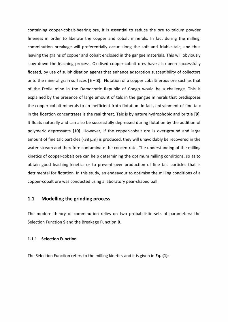
The Selection Function refers to the milling kinetics and it is given in Eq. (1):

αaxiS =Λ

xi1+μ

(1)

where xi is the upper limit of the particle size interval under consideration; the model

parameters a and μ are mainly functions of the grinding conditions while α and Λ are

material properties.

Fig. 1 hereunder shows the first-order breakage law for a given material. The initial straight

line portion of the curve which shows the normal breakage behaviour is the area where S

has not passed through the maximum. The second portion, area where S has passed the

maximum, shows the abnormal breakage behaviour. According to Griffith theory of

breakage [11], this trend can be attributed to the fact that very fine particles are hard to

break. The breakage rate is also affected by the reduced capture probabilities of fine

particles in mills [12]. This suggests that the breakage rate increases with increase in particle

size. However, for too large particles that cannot be correctly nipped and fractured by the

balls, the rate of breakage steadily drops and tends to zero.

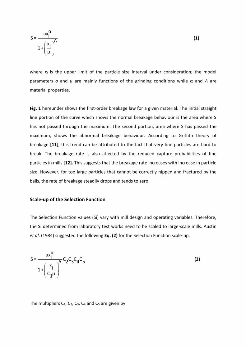
Scale-up of the Selection Function

The Selection Function values (Si) vary with mill design and operating variables. Therefore,

the Si determined from laboratory test works need to be scaled to large-scale mills. Austin

et al. (1984) suggested the following Eq. (2) for the Selection Function scale-up.

αaxiS = C C C C4 52 3Λxi1+

C μ1

(2)

The multipliers C1, C2, C3, C4 and C5 are given by

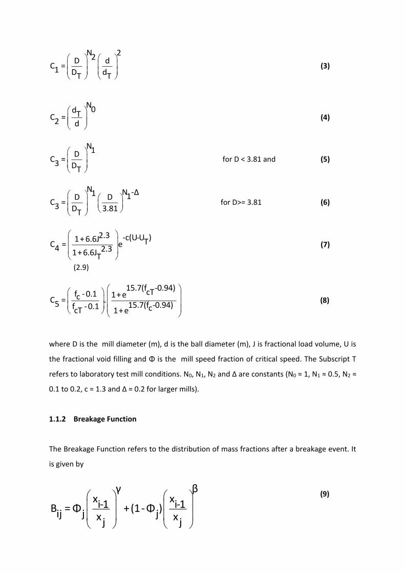
N 22D dC =1 D dT T

(3)

N0dTC =2 d (4)

N1DC =3 DT

for D < 3.81 and (5)

N N -Δ1 1D DC =3 D 3.81T

for D>= 3.81 (6)

2.3 -c(U-U )1+ 6.6J TC = e4 2.31+ 6.6JT

(7)

(2.9)

15.7(f -0.94)cTf - 0.1 1+ ecC = .5 15.7(f -0.94)f - 0.1 ccT 1+ e (8)

where D is the mill diameter (m), d is the ball diameter (m), J is fractional load volume, U is

the fractional void filling and Φ is the mill speed fraction of critical speed. The Subscript T

refers to laboratory test mill conditions. N0, N1, N2 and Δ are constants (N0 ≈ 1, N1 ≈ 0.5, N2 ≈

0.1 to 0.2, c = 1.3 and Δ = 0.2 for larger mills).

1.1.2 Breakage Function

The Breakage Function refers to the distribution of mass fractions after a breakage event. It

is given by

(9)

γ βx xi-1 i-1B =Φ +(1-Φ )ij j jx xj j

where Φ, γ and β are the model parameters that depend on the ore properties. xi is the

particle size in the ith class of breakage progeny and xj the particle size of the size being

broken.

The Bij values are said to be normalisable if the breakage distribution function is

independent of the initial particle size (Austin et al., 1984). In other words, the fraction

which appears at sizes less than the starting size is independent of the starting size. For

normalized B values, δ=0 and the Bij are superimposed upon each other.

A graphical illustration of the cumulative breakage distribution function based on Eq. (9) is

given in Fig. 2. The distribution is in fact a simple weighted sum of two Schuhmann

distributions (straight line plots on a log-log scale). The slope of the lower portion of the curve

gives the value of γ , the slope of the upper portion of the curve gives the value of β , and j is

the intercept of the lower portion of the curve at xj [11].

1.1.3 Batch Grinding Equation

The knowledge of the Selection and Breakage functions enables the prediction of particle

size distribution for a given ore sample. [11] procedure which consists in a series of

laboratory tests in a small mill using a one-size-fraction method is often used. The material

is loaded in the mill together with the ball media. Then the grinding is performed for several

suitable grinding time intervals. After each interval, the product is sieved. Thus the

disappearance rate of feed size material is calculated for the different grinding time

intervals. By performing a population balance at size class i in which the selection and

breakage functions are incorporated, one gets

dw (t) i-1i = -S w (t)+ b S w (t)i i i,j j jdt j=1

i 1

, n i j 1 (10)

2. Experimental

2.1 Description of the experimental laboratory mill

An experimental laboratory scale ball mill available at the University of Lubumbashi was

used in this research work. The ball mill measured 0.305 m in diameter and 0.127 in length.

It was driven by an asynchronous motor rated with power close to 10 kW. A schematic of

the experimental laboratory ball mill used is shown in Fig. 3.

2.2 Sample preparation

The copper-cobalt ore used in the actual test work was obtained from the feed to the

primary mill (run of mine) at the Etoile mine of Rwashi mining, a subsidiary of the Metorex

group. The ball mill feed content mass was calculated using following

.

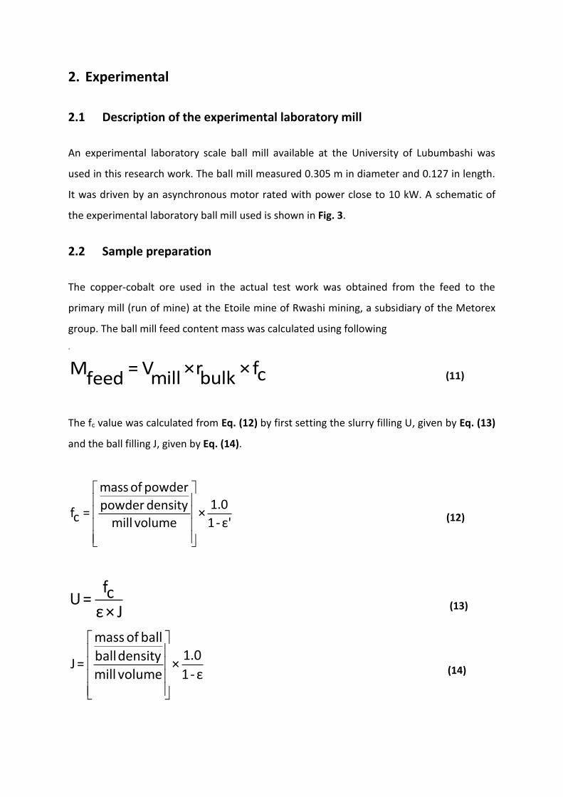
M = V ×r × fcmill bulkfeed (11)

The fc value was calculated from Eq. (12) by first setting the slurry filling U, given by Eq. (13)

and the ball filling J, given by Eq. (14).

mass of powder1.0powder density

f = ×c mill volume 1-ε' (12)

fcU=ε× J (13)

mass of ball1.0ball density

J = ×mill volume 1-ε (14)

where

Slurry filling (U) is the fraction of the spaces between the balls at rest which is filled with

slurry. Mill filling (fc) is expressed as the fraction of the mill volume filled by slurry bed using

a slurry bed porosity ε. Ball filling (J) is expressed as the fraction of the mill volume filled by

the ball bed at rest, assuming a bed porosity ε’. In this work, the slurry bed porosity and ball

bed porosity were chosen equal to 0.4 that is the conventionally formal bed porosity.

2.3 Laboratory operating conditions Table 1 gives the laboratory and industrial operating conditions.

2.4 Milling Kinetics tests The one-size fraction method by Austin et al. (1984) for measuring the Selection and

Breakage Functions was used to determine the breakage and selection function parameters.

Twelve mono sized fractions were prepared and wet ground batch wise using a laboratory-

scale ball mill at the University of Lubumbashi: -6700 + 4750 µm, -4750 + 3350 µm, -3350 +

2360 µm, -2360 + 2000 µm, -2000 + 1700 µm, -1700 + 1400 µm, -1400 + 1000 µm, -1000 +

850 µm, -850 + 500 µm, -500 + 250 µm, -250 + 125 µm and -125 + 75 µm. After the sample

and the balls were loaded to the ball mill, it was run for seven different time intervals (½, 1,

2, 4, 8, 15 and 30 minutes). The total individual composite samples for each test were

carefully removed from the mill. They were weighed in the collection bucket while wet; then

pressure filtered, using tared filter paper before being placed on a pan and finally in an oven

for drying over night at a temperature of about 65°C. The dried samples were then re-

weighed and a representative sample was taken for particle size distribution determination.

Then, the feed for the next grinding period was the material retained on the screens,

combined with the rest of the mill contents.

2.5 Simulation of the grinding process

The Matlab simulator code by [13] that directly translates the population balance model

(Eq. (10)) was used to generate the simulated product size distributions. Details on the

Matlab code used can be found in Appendices A.1-A.3.The flowchart of the calculation

procedure is shown in Fig. 4. In order to tune this simulator with the actual grinding process,

the breakage function parameters (β, γ and Φ) and selection function parameters (α),

determined from the experimental tests according to the one-size method by [11], were

pre-entered into the code. The remaining selection Function parameters (a, Λ and µ) were

then estimated by the simulator by minimising the sum of squared errors (SSEs) between

the predicted and experimental product size distributions. Finally, the bi,j functions were

then back-calculated by the simulator.

3. Results and discussions

3.1 Determination of the Selection Function parameters

The size-dependence of the Selection Function parameters Eq. (1) was used to derive

numerically the rate of breakage of the copper-cobalt ore. Experimental mass percents

retained on the top screen were plotted against the grinding time t on a log-linear scale for

all feed sizes. To illustrate this, the first order grinding plots of the copper-cobalt for

selected mono sized fractions (-250 + 125 µm, -3350 + 2360 µm and -6700 + 4750 µm) are

shown in Figs. 5-7. The results in Table 2 indicate that the magnitudes of the Selection

Function increased with the increase in the size of particles; but quickly decreased beyond

1700 µm.

The Selection Function values were plotted in Fig. 8. It can be seen that the Selection

Function curve presents two regions: a low-particle-size linear region and an upper non-

linear region. The graphical procedure of the full determination of all parameters associated

with the Selection Function is given in Fig. 1 [11]. With respect to the data outlined in this

article, the Selection Function curve was assumed to be linear up to 1700 µm, where the

maximum value of S occurred. In other words, the media were large enough to break

efficiently the particles in this region. With a further increase in the particle size, the ore

sample was too big and strong to be properly nipped and fractured by the actual ball

distribution. Hence, the breakage took place in the abnormal breakage region. As a result,

the specific rates of breakage decreased. The value of alpha (α) was then determined from

the linear region in Fig. 8, by using a power function. This value was fed into the population

balance model for the computer simulations.

The Selection Function parameters are summarized in Table 3.

The specific rates of breakage determined in the laboratory ball milling tests were scaled-up

to the industrial scale mill using Eq. (2). The multipliers used to scale-up the selection

functions were calculated by using Eqs. (3) - (8). The multipliers obtained are C1=18.343,

C2=0.275, C3=2.999, C4=1.016 and C5=1.563. Only the model parameters a and μ are affected

by the multipliers (a for Si scaled-up: supa = a.C .C .C .C4 52 3 ,µ for Si scaled-up: supμ

μ =C1

),

since they depend on the grinding conditions. The remaining Selection Function parameters

(α and Λ) are material properties. The scaled-up Selection Function parameters are

presented in Table 4.

3.2 Determination of the Breakage Function parameters The B-II calculation procedure of the primary breakage function as proposed by [11] was

used to generate the Breakage Function parameters. This method suggests the use of

shorter grinding times, which result in 20–30% broken materials out of the top size before

re-breakage. [3] further stated that up to 65% broken material will still provide accurate

data to be used with this procedure. All the feed materials were considered to be

normalizable (δ = 0) for simulation purposes. This means that the fraction appearing at sizes

less than the initial feed size was independent of the initial feed size. The cumulative

breakage distribution functions of the copper-cobalt ore at different initial feed sizes are

shown in Fig. 9.

The Bij values obtained were fitted to the empirical model in Eq. (9) [11], and the model

parameters: β, γ and φ for the UG2 ore were evaluated. The Breakage Function parameters

are listed in Table 5. The average Breakage Function values obtained are β = 5.20, γ = 1.01

and Φ = 0.86. These values parameters are a little different with those obtained by [14] for a

copper ore in a VertimillTM pilot test, which were: β = 3.33, γ = 0.615 and Φ = 0.463. This was

believed to be due to the presence of high talc content in the copper-cobalt ore sample

treated. [15] also found values of β = 4.0, γ = 0.60 and Φ = 0.45; based on their ball milling

experiment on copper ore sample from the Los Broncos mine.

3.3 Particle size distributions The parameters (α, Λ, γ and µ) were estimated by the optimization model that seeks the

best combination of these parameters in order to minimize the residual error between the

experimental and predicted product size distributions. The parameters of the Selection and

Breakage Functions evaluated from the experimental data were used as initial guesses to

the model in the parameter search process. The average Breakage and Selection Functions

parameters were then used to obtain the product size distribution (PSD) of a normal

copper-cobalt ore (un-sized) that was milled for ½, 1, 2, 4, 8, 15 and 30 minutes. The

measured and predicted size distributions for all the milling products are given in Fig. 10. It

can be seen that there is a fair agreement between the measured size distributions, shown

as markers in the plotted graphs, and the simulated size distributions, shown as solids lines.

This allowed validating the kinetics model and suggested that the Selection and Breakage

Functions parameters obtained can be used for continuous operation mass balance.

4. Conclusion

An understanding of the milling kinetics of the Etoile mine copper-cobalt ore is being

improved. The simulations indicated that is possible to predict the particle size of a pear-

shaped ball mill using the population balance model. The milling kinetics model developed

can be useful to provide insight into the copper-cobalt ore behaviour in milling circuits by

using routine laboratory batch milling test results. Such information can also be

implemented on the grinding circuit models in order to improve actual industrial copper-

cobalt ore flowsheets.

5. Acknowledgements

The authors are grateful to the management of Rwashi mining for the donation of the

copper-cobalt ore sample that was used in this work and for having granted them access to

the technical data of the milling circuit.

6. References

[1] Rhodes M. Introduction to Particle Technology. John Wiley and Sons, Chichester. 1998.

[2] Walkiewicz JW, Lindroth DP, Clark AE. Iron ore grindability improved by heating.

Engineering & Mining Journal 1996;197:p16CC.

[3] Austin LG, Luckie PT. The Estimation of non-normalized breakage distribution

parameters from batch grinding tests. Powder Technology 1972;5:215–222.

[4] Bingöl D, Canbazoğlu M. Dissolution kinetics of malachite in sulphuric acid.

Hydrometallurgy 2004;72:159–165.

[5] Kongolo K, Kipoka M, Minanga K, Mpoyo M. Improving the efficiency of oxide copper-

cobalt ores flotation by combination of sulphidisers. Minerals Engineering 2003;16:1023–

1026.

[6] Ziyadanogullari R, Aydin F. A new application for flotation of oxidized copper ore. Journal

of Minerals and Materials Characterization and Engineering 2005;4:67-73.

[7] Lee K, Archibald D, Reuter MA. Flotation of mixed copper oxide and sulphide minerals

with xanthate. Minerals Engineering 2009;22:395–401.

[8] Tebogo PP, Muzenda E. A multistage sulphidisation flotation procedure for a low grade

malachite copper ore. International Journal of Chemical, Nuclear, Metallurgical and

Materials Engineering 2010;4.

[9] McHardy J, Salman T. Some aspects of the surface chemistry of talc flotation.

Department of mining and metallurgical engineering, McGill University, Montreal, Quebec,

Canada. 1974.

[10] Morris, G.E., Fornasiero, D., and Ralston, J. Polymer depressant at the talc-water

interface: adsorption isotherm, microflotation and electrokinetic studies. International

journal of mineral processing 2002;67:211-227.

[11] Austin LG, Klimpel RR, Luckie PT. Modelling for Scale- up of Tumbling Ball Mills: Control

’84. Society of Mining Engineers of the AIME 1984.

[12] Tangsathitkulchai C. Acceleration of particle breakage rates in wet batch ball milling.

Powder Technology 2002;124:67– 75.

[13] Bwalya M. Population Balance Simulator code. School of Chemical and Metallurgical

Engineering, University of the Witwatersrand. 2012.

[14] Mazzinghy DB, Galéry R, Schneider CL, Alves VK. Scale up and simulation of VertimillTM

pilot test operated with copper ore. Journal of materials research and technology

2014;3:86–89.

[15] Tangsathitkulchai C, Austin LG. The Effect of Slurry Density on Breakage Parameters of

Quartz, Coal and Copper Ore in a Laboratory Ball Mill. Powder Technology 1985;42:287-296.

7. Appendices