Appl. Sci. 2020, 10, 6036; doi:10.3390/app10176036 www.mdpi.com/journal/applsci

Article

Determination of Axial Force in Tie Rods of Historical Buildings Using the Model-Updating Technique Ivan Duvnjak, Suzana Ereiz, Domagoj Damjanović and Marko Bartolac *

Faculty of Civil Engineering, University of Zagreb,1000 Zagreb, Croatia; ivan.duvnjak@grad.unizg.hr (I.D.); suzana.ereiz@grad.unizg.hr (S.E.); domagoj.damjanovic@grad.unizg.hr (D.D.) * Correspondence: marko.bartolac@grad.unizg.hr

Received: 7 August 2020; Accepted: 28 August 2020; Published: 31 August 2020

Abstract: Tie rods are structural elements that transfer axial tensile loads and are typically used on walls, vaults, arches, and buttresses in historical buildings. To verify their load-bearing capacity and identify possible structural damage risks, the forces transferred by tie rods and the corresponding stresses must be determined. However, this is often a challenging task due to the lack of project documentation for historical buildings. Uncertainties like complex boundary conditions or unknown material and geometrical properties make it hard to assess the tie rods’ load level. This paper presents a methodology for the determination of axial forces in tie rods that combines on-site experimental research and a numerical model-updating technique. Along with the common approach based on a determination of the natural frequency of tie rods, this paper presents an approach based on tie rods’ mode shapes. Special emphasis is placed on the boundary conditions coefficient, which is a crucial parameter in the analytical solution for axial forces determination based on the conducted on-site experiments. The method is applied in a historical building case study.

Keywords: tie rod; structural health monitoring (SHM); natural frequencies; mode shapes; root-mean-square error (RMSE)

1. Introduction

Displacements that occur with historical buildings can be arrested using metal beams, or tie rods, which support the masonry walls, buttresses, arches, and vaults in the plane of bending out. Tie rods are subjected to axial tension and are an essential element in the control of horizontal forces (displacements) produced by static and dynamic loads related to seismic actions. In extreme cases, a tie rod can reach its maximum bearing capacity due to high stress or the pulling out of its anchor point. Both scenarios can lead to a loss of structural integrity. Therefore, the value of the internal tensile force in tie rods is a frequent subject of discussion. Figure 1 represents a typical tie rod in historically-important buildings such as cathedrals, churches, or castles.

Figure 1. Cathedral of St. James in Šibenik (Croatia). Tie rods are supporting the walls and arches.

Appl. Sci. 2020, 10, 6036 2 of 15

Several uncertainties exist when determining the forces in tie rods, including complex boundary conditions [1–3] and geometrical and material properties [3,4]. Boundary conditions can vary, ranging from theoretically-fixed and pinned conditions to those that should be considered with spring elements (Figure 2). In practice, the length of the anchoring of the tie rod is associated with geometrical problems. Due to the limitations of inspection, material properties such as the Young’s modulus are often unknown. Evaluation of tensile forces in tie rods can be achieved using static, dynamic, or mixed approaches.

Figure 2. Examples of complex (unclear) boundary conditions.

Two static approaches can be used for the determination of tensile forces in tie rods. The first involves loading of the tie rod in several stages and then measuring deflections and strains in representative locations [5–7]. The second approach is known as the residual stress method [8]. This involves attaching strain gauge rosettes to the surface, drilling a hole at the center of the gauge, and measuring the residual strain caused by the relaxation of the material surrounding the drilled hole. The several disadvantages to static approaches include the following:

• The tie rods are generally located at elevated positions; • High-accuracy displacement sensors should be used due to small vertical displacements. These

should be placed on a previously-determined referent location; • The strain gauge installation can be complicated at elevated positions.

The aforementioned approaches require considerable time for application and they are slightly destructive. Based on the mentioned disadvantages, many authors have researched a dynamic approach based on numerical or analytical methods [9–11].

Vibration-based methods (dynamic approach), as nondestructive methods, are widely applied for the evaluation of axial forces in tensile elements of structures. These methods are mainly based on tie rods’ natural frequencies, which are later used for the determination of forces. A distinction must be made between transverse oscillations of strings and beams. String theory is widely used for the determination of cable forces in structures such as bridges [12] due to the high ratio of length to cross-section dimensions. Unlike beam theory, string theory does not consider the flexural stiffness or boundary conditions [13,14].

Tensile forces in tie rods can also be evaluated using a mixed approach. This approach is a combination of previously-mentioned approaches—static- and vibration-based. In this case, tie rods are modeled as simply supported Euler beams with rotational springs with unknown stiffness on each edge [15]. Besides the stiffness of rotational springs, the second unknown parameter is force. These unknown parameters are obtained by solving a system of equations composed of static equations for deflection and dynamic equations for natural frequencies. This method requires data from two separate experiments. The first experiment involves measuring the deflection in representative locations on a beam and the second involves measuring the natural frequency. Although a mixed approach showed good results in laboratory conditions, measurement errors can cause a significant deviation in results. If the number of unknown parameters is larger, the probability

Appl. Sci. 2020, 10, 6036 3 of 15

of error is also greater. Although there are two such parameters in this case, they are enough to cause a significant deviation in the results [16–18].

In this study, a combination of experimental and numerical research was used for the determination of forces in tie rods based on the natural frequencies (fn), flexural stiffness (EI), mass (m), and boundary conditions. The method was verified on a historical building case study. One characteristic tie rod in this building was analyzed in detail. Based on these analyses of the characteristics of a single tie rod and the experimentally-determined values of the natural frequencies on the other tie rods in the building, the force in all the tie rods was determined reliably.

The remainder of this paper is structured as follows: Section 2 presents an analytical solution for lateral vibration of a tie rod and provides an equation for the determination of the tensile force, Section 3 describes the proposed methodology in detail, and Section 4 presents the application of the proposed methodology on a real historical building.

2. Analytical Solution for Lateral Tie Rod Vibration

As discussed above, the natural frequencies of a tie rod depend on three basic assumptions—axial load, stiffness, and boundary conditions. The lateral vibrations of the tie rod are assumed as a superposition of two solutions—the lateral vibrations of the Euler‒Bernoulli beam (considering stiffness) and the lateral vibration of string (considering the axial effect). The boundary conditions are considered in the proposed solutions of differential equations.

Figure 3a depicts small-amplitude free lateral vibration with a uniform cross-section of the beam with material density ρ. In the cross section, dx is the acting internal forces (P) with a positive orientation, including the weight of beam caused by vibrations (Figure 3b).

Figure 3. (a) Beam under lateral vibration and axial loading and (b) differential segment of beam representing the positive orientation of bending moments, shear forces, and axial and inertial forces of mass.

Shear forces (Vz) are acting in a vertical direction of an element and are responsible for balancing a weight of segment that varies in time along with element ( ρ ∂ ∂2 2dx w/ t ). The sum of vertical forces is equal to the product of the mass of the element and acceleration (Equation (1)):

∂ ∂= → −ρ − + = ∂∂

2Z

Z Z2

Vwz 0 V dx V dx 0xt

,

∂ ∂= −ρ∂ ∂

2Z

2

V w x t

.

(1)

If the moments are taken about point C of the element dx (Equation (2a)), the term contains vertical forces (Vz and Pz) and axial bending moment (My). Substituting the bending moment with flexural stiffness (EI) and taking the second derivative of the deflection of beam ( 2 2

yM EI w / x= − ∂ ∂

) and a component of axial force Pz = Ptgα = P∂w/∂x, Equation 2b gives Equation (3)

Appl. Sci. 2020, 10, 6036 4 of 15

∂ ∂ = → + + − + + + + = ∂ ∂

y Zc y Z Z y Z z

M Vdx dx dx dxM 0 M V P M dx V dx P 02 2 x x 2 2

,

∂+ − =

∂y

Z z

Mdx dx2V 2P dx 02 2 x

,

(2a)

∂ ∂= −∂ ∂

yZ

M wV Px x

, (2b) ∂∂ ∂= −

∂ ∂ ∂

2 2yz

2 2

MV wPx x x

, (2c) ∂ ∂ ∂= − −∂ ∂ ∂

4 2z

4 2

V w wEI Px x x

. (3)

Finally, substituting Equation (3) into Equation (1) provides the basic equation for lateral vibration of the beam with inner constant axial force (Equation (4)):

∂ ∂ ∂+ −ρ =∂ ∂ ∂

4 2 2

4 2 2

w w wEI P 0x x t

. (4)

The solution of this equation can be expressed as a form of harmonic functions of w(x,t) (Equation (5)) or in terms of exponential functions. For the selected function, constants (A, B, C, and D) should be found considering various boundary conditions with applying known conditions to the deflection, slope, bending moment, and shear forces: 𝑤 𝐴 cos 𝜅𝑥 cosh𝜅𝑥 𝐵 cos𝜅𝑥 cosh𝜅𝑥𝐶 sin𝜅𝑥 sinh 𝜅𝑥 𝐷 sin𝜅𝑥 sinh 𝜅𝑥 . (5)

Ultimately, a natural frequency for the nth mode shape in tie rods can be determined according to [19,20] as

κ= +π π

2 2

n 2 2 2

EI Plf 1m '2 l EI n

, (6)

where n is the mode shape number, fn is the nth natural frequency, l is a span of tie rod, m’ is mass per unit length ( =ρm' bh , b—width, and h—height of cross section) and κ is a boundary condition parameter, as presented in Table 1. By rearranging the previous equation, the boundary conditions (κ) can be determined:

πκ =

+π

2n

2

2 2

f 2 l

EI Plm ' m ' n

(7)

Table 1. Value of boundary condition parameter κ for the first two [19] and nth [20] natural frequencies having various boundary conditions

Boundary Condition

Static System Coefficient κ

1st Mode 2nd Mode nth Mode Hinge–hinge 3.142 6.283 ≅ πn

Clamp–clamp

4.730 7.853 ( )+≅ π

2n 12

Clamp–hinge

3.927 7.069 ( )+≅ π

4n 14

Clamp–free

1.875 4.694 ( )−≅ π

2n 12

Appl. Sci. 2020, 10, 6036 5 of 15

Based on known natural frequencies (fn), properties (EI, m’), and boundary conditions (κ), we can determine the axial force of a tie rod:

π= − πκ

4 22 2 2 2n4 2

n EIP 4f m'l nl

. (8)

Although the previous equation is simple, it only considers ideal boundary conditions. Generally, in real life, the boundary conditions are quite complicated and very often nonsymmetrical problems. This is why we assessed the axial forces in tie rods using analytical solutions, experimental research, and numerical analysis.

3. Methodology for Boundary Conditions and Axial Load Identification

The proposed methodology is composed of three stages divided into experimental research on-site and numerical optimization, considering an analytical solution for the determination of axial force (Figure 4). The experimental research (stage 1) involved vibration-based measurement [21] of natural frequencies, exp

nf , and mode shapes determination by using operational modal analysis (OMA) [22,23]. Based on the assumed boundary conditions, known materials, and geometric properties, an initial numerical model of a tie rod was developed (Figure 4, stage 2). Mode shapes from the numerical simulation and experiments were compared using normalized root-mean-square error (RMSE) [24], as presented in Equation (9):

RMSE = , ,( ) , (9)

where n is the mode shape number, Φnumn ,j is the numerically-obtained normalized mode shape

vector, and Φ expn , j is the experimentally-obtained operating deflection shape at the jth point on the tie

rod. Based on the RMSE values, the numerical model was updated by adapting the boundary conditions (BC). When the RMSE reached its minimum value, it indicated that the experimental and numerical mode shapes were overlapping, which ultimately meant that boundary conditions were updated adequately (Figure 4, stage 2—updated model BC). Finally, based on known natural frequencies from on-site measurements, exp

nf , and a previously-updated numerical model, the axial

force was tuned to a numerical model to match the natural frequency, numnf , with that from an

experiment, expnf (Figure 4, stage 2—updated model (BC + num

nf ). Using this procedure, considering experimental measurements, and updating the numerical model, the axial force (P) was determined (Figure 4, end of stage 2).

Appl. Sci. 2020, 10, 6036 6 of 15

Figure 4. Methodology for boundary conditions determination.

Generally, the simulated boundary conditions in the numerical model are complicated and do not coincide with the basic support conditions given in Table 1. Hence, by applying known geometrical and material properties with the resulting axial force in an analytical solution (Equation (7)), we can determine the coefficient κ, which is associated with the boundary conditions (Figure 4, stage 3). Using this methodology on one characteristic tie rod, a boundary coefficient was determined and this value can then be applied to other tie rods with the same boundary conditions (Figure 5). Therefore, it is sufficient to perform on-site measurements of the natural frequencies in each tie rod to determine the axial force (Figure 5, end of stage 3). In case of varying boundary conditions for tie rods in the building, the numerical model updating should be applied to each tie rod (stages 1 and 2) without determination of coefficient κ.

Figure 5. Methodology for axial load identification.

4. Case Study Using the Proposed Methodology

The previously-described methodology (Figures 4 and 5) was applied to a historical building case study. The Cathedral of St. James in Šibenik (Figure 6), Croatia, is a good example of a historical building with defined dynamic tie rod parameters (frequencies and mode shapes). For the sake of simplicity, one of the tested iron tie rods was taken as a reference for which we conducted a detailed analysis.

4.1. Description of Structure

The Cathedral of St. James in Šibenik, Croatia, is a unique architectural work whose construction began in 1431 and lasted almost 100 years. The cathedral was built exclusively of stone and marble, without brick, wood, or concrete as binders. The cathedral is shaped like a Latin cross, divided by

Material and geometrical properties

Natural frequencies (fnexp)

Boundary conditions κ

STAGE 1 STAGE 3

Axial force P (Eq. 8)

ON SITE MEASUREMENTS

Legend:

Start

Output

Appl. Sci. 2020, 10, 6036 7 of 15

arcades into a three-nave structure. The medium-sized nave, which is tall and illuminated, holds 12 Gothic columns, whereas the lateral naves are darker and lower. Data regarding the geometry of the cathedral can be found in a previous study [25]. In 2001, the Cathedral of St. James was given UNESCO World Heritage status.

(a) (b)

Figure 6. Cathedral of St. James in Šibenik, Croatia. (a) West view of cathedral and (b) iron tie rods inside the cathedral.

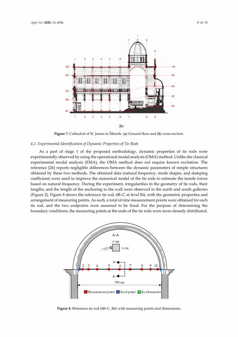
The system of tie rods in the Cathedral of St. James in Šibenik consists of iron and aluminum tie rods set in the three levels of the cathedral. At the abutment of the central barrel vault, nine iron tie rods are connected at level R4 (Figure 7). The columns and vaults of the gallery are connected by 24 aluminum tie rods shorter than the tie rods of the central barrel vault. Aluminum tie rods are placed in the transverse direction (axis 1‒7, from A to B and from C to D) and in the longitudinal direction (axis B and C, from 1 to 7) at the R2 level (Figure 7). The iron tie rods were the focus of the research.

(a)

Appl. Sci. 2020, 10, 6036 8 of 15

(b)

Figure 7. Cathedral of St. James in Šibenik. (a) Ground floor and (b) cross-section.

4.2. Experimental Identification of Dynamic Properties of Tie Rods

As a part of stage 1 of the proposed methodology, dynamic properties of tie rods were experimentally observed by using the operational modal analysis (OMA) method. Unlike the classical experimental modal analysis (EMA), the OMA method does not require known excitation. The reference [26] reports negligible differences between the dynamic parameters of simple structures obtained by these two methods. The obtained data (natural frequency, mode shapes, and damping coefficient) were used to improve the numerical model of the tie rods to estimate the tensile forces based on natural frequency. During the experiment, irregularities in the geometry of tie rods, their lengths, and the length of the anchoring to the wall were observed in the north and south galleries (Figure 2). Figure 8 shows the reference tie rod, 6B‒C at level R4, with the geometric properties and arrangement of measuring points. As such, a total of nine measurement points were obtained for each tie rod, and the two endpoints were assumed to be fixed. For the purpose of determining the boundary conditions, the measuring points at the ends of the tie rods were more densely distributed.

Figure 8. Reference tie rod (6B‒C, R4) with measuring points and dimensions.

Appl. Sci. 2020, 10, 6036 9 of 15

For simplicity, tie rod 6B‒C was taken as the reference, and a more detailed analysis was performed on it, as follows: The on-site measurements were performed using five piezoelectric accelerometers (Brüell & Kjaer, Denmark, type 4508-B, nominal sensitivity 100 mV/g). The OMA was conducted by roving four accelerometers through two measuring stages, using one as a referent. The tie rods were excited by randomly using a rubber impact hammer. Frequency domain decomposition (FDD) and enhanced frequency domain decomposition (EFDD) were used for the estimation of modal parameters (Figure 9). The values of the experimentally-obtained frequencies for the concerned mode shapes were read from the characteristic record (Figure 10).

Figure 9. The first two experimentally-obtained mode shapes of the reference iron tie rod 6B‒C.

Figure 10. Characteristic record of frequency domain decomposition (FDD) for the determination of natural frequencies on reference iron tie rod 6B‒C.

The natural frequencies of the remaining tie rods were measured using only one accelerometer placed at the node 4 (Figure 8). Geometric properties (L—length, b—width, and h—height) and the first two experimentally-obtained natural frequencies (fnexp, n = 1, 2) for the observed tie rods are presented in Table 2. Please note that the cross-section dimensions present an average value of five measurements performed in quarters of tie rods’ length.

Table 2. Values of the first two frequencies of experimentally-observed tie rods in the Cathedral of St. James in Šibenik at level R4.

Tie Rod L (m)

h (mm)

b (mm)

f1exp (Hz)

f2exp (Hz)

2B‒C 6.84 55 55 7.25 17.94 3B‒C 6.71 64 64 7.56 19.00 4B‒C 6.81 60 60 7.31 18.69 5B‒C 6.87 68 68 7.31 19.56 6B‒C 6.90 61 61 6.94 17.50 7B‒C 6.95 56 56 8.25 18.88 7‒8B 6.97 56 56 8.13 19.38 7‒8C 6.98 60 60 8.63 19.38

Appl. Sci. 2020, 10, 6036 10 of 15

4.3. Numerical Simulation

The numerical model of the tie rod was developed as the Euler‒Bernoulli beam element in SAP2000 software (Computers and Structures, Walnut Creek, CA, USA). The geometrical characteristics of tie rods—width and height—were assumed to be constant over their entire length and the rods were assumed to be homogenous throughout their volume. The material properties were based on literature review and taken as invariable; the elastic modulus E was considered as 185 GPa, the Poisson coefficient ν as 0.3 and material density ρ as 7850 kg/m3. Once the modal parameters were experimentally obtained, a numerical model was updated while changing the boundary conditions from fixed to hinged. To construct a real-life model, boundary conditions were additionally tuned with spring coefficients (stage 2 of the proposed methodology).

4.3.1. Initial Model

The initial numerical model was constructed to determine the deviation of the real state of the structure from the ideal boundary conditions (clamp and hinge) and to evaluate which of those boundary conditions better described the real state. The finite element (FE) distribution of the numerical model corresponded to the arrangement of the measuring points shown in Figure 8. For each initial model, the first two natural frequencies and mode shapes were determined (Figure 11).

(a) (b)

Figure 11. Comparison of the experimental mode shapes of the reference tie rod 6B‒C and the mode shapes associated initial numerical models for the (a) first and (b) second mode shapes.

To avoid subjective assessment of the boundary conditions, mode shapes from numerical simulation and experiments were compared using normalized RMSE (Equation (9)). For each initial numerical model and its corresponding mode shapes, the RMSE values were determined. Based on the RMSE values (Table 3), we observed that the initial model with hinged boundary conditions better correlated (values approaching 0) with the on-site measurements. Based on the results, hinged boundary conditions were identified as a good selection for the initial model and were further updated by adapting the spring stiffness on the boundary.

Table 3. Root-mean-square error (RMSE) values for initial numerical models for two mode shapes.

RMSE Values Mode Number Hinge–Hinge Clamp–Clamp

1 7.06 9.15 2 8.50 10.66

Appl. Sci. 2020, 10, 6036 11 of 15

4.3.2. Updated Model

When updating the numerical model of tie rods, rotational springs were added at each boundary, starting from the initial hinged model. Spring stiffness was determined by an iterative procedure. Their values were changed until the mode shapes of the numerical model entirely corresponded to the mode shapes obtained by on-site measurements. During the iteration, the change in the RMSE value was monitored depending on the change of the spring stiffness (k) (Figure 12). Through several iteration steps, due to the minimum value of RMSE, it was possible to select the appropriate spring stiffness for each mode shape. In this way, the finite element (FE) model was updated to overlap with the experimental model considering only the boundary conditions.

Figure 12. The values of the RMSE for the observed mode shapes and different spring stiffness values.

Table 4. shows the natural frequencies computed by SAP2000 (fnnum) and the relative error between these frequencies and the frequency values determined by on-site measurement (fnexp). The error varied between 20% and 30% for the first two frequencies, which confirmed the assumptions about the axial force in the tie rods.

Table 4. Values of experimentally-measured natural frequencies and computed frequencies (fnnum) for the updated numerical model.

Mode Number fnnum (Hz)

fnexp (Hz)

Relative Error (%)

1 4.83 6.94 30.20 2 13.95 17.50 20,29

Therefore, the next step was to adjust the natural frequencies of the numerical model to correspond to those obtained from on-site measurements. The natural frequencies were adjusted by changing the tension in the FE model of the tie rod. In addition, the procedure of tuning natural frequencies is iterative, and it was implemented for the first two mode shapes. The values of experimentally-measured natural frequencies (fnexp) were compared to the numerical model (fnnum) and are presented in Figure 13. After tuning the tension for both mode shapes (P1, P2) in the FE model, the results of natural frequencies were in good agreement with those measured for both mode shapes (Figure 13). The tuning of dynamic properties of the FE model enabled us to determine the actual tension in the tie rod (Table 4).

Appl. Sci. 2020, 10, 6036 12 of 15

Figure 13. Change of force values depending on the ratio of numerical and experimental frequency values for two mode shapes (P1, P2).

Based on the proposed methodology, we continued to the final stage (stage 3) of determination of axial force and coefficient κ. With known axial force (from the updated numerical model) and geometrical and material properties (from on-site observations), coefficient κ could be determined by using Equation (7). As expected, the values of coefficient κ (Table 5) obtained for both mode shapes were within the theoretical boundaries of the hinge–hinge and clamp–clamp conditions previously presented in Table 1. Based on the force values obtained from two mode shapes indicated in Table 5, one can observe that there is a difference of around 12% between these values. It can be concluded that the force value varies depending on the number of the observed mode shapes as indicated in [27].

Table 5. The force values read for the first two mode shapes and the value of coefficient κ determined by the calculation of the updated model.

Mode Number fnnum

(Hz) P

(kN) σ

(MPa) κ

1 6.94 122.8 33.0 3.534 2 17.5 137.2 36.9 6.777

We assumed that the coefficient κ found by using this procedure could be applied to all remaining tie rods. The stated assumption was based on the on-site visual inspection and the observed geometrical and material properties.

Based on the defined coefficient κ, experimentally-determined natural frequencies, and analytical equations, the values of the axial forces and the stress levels (Table 6) were determined for the observed iron tie rods in the Cathedral of St. James in Šibenik, Croatia.

Table 6. The value of forces Pn (kN) and stress levels σn (MPa) for the observed mode shapes in the tie rods observed in the Cathedral of St. James in Šibenik at level R4.

2B‒C 3B‒C 4B-C 5B-C Mode Num.

κ Pn

(kN) σn

(MPa) Pn

(kN) σn

(MPa) Pn

(kN) σn

(MPa) Pn

(kN) σn

(MPa) 1 3.534 115,8 38,3 149.6 36.5 132.1 36.7 159.4 34.5 2 6.777 144.7 47.8 158.8 38.8 167.7 46.6 207.9 45.0 Mean values 130.3 43.1 154.2 37.7 149.9 41.6 183.6 39.7 6B‒C 7B‒C 7‒8B 7‒8C

Mode Num.

κ Pn

(kN) σn

(MPa) Pn

(kN) σn

(MPa) Pn

(kN) σn

(MPa) Pn

(kN) σn

(MPa) 1 3.534 122.8 33.0 170.8 54.5 166.3 53.0 215.2 59.8 2 6.777 137.2 36.9 188.7 60.2 208.1 66.4 219.6 61.0 Mean values 130.0 34.9 179.8 57,3 187.2 59.7 217.4 60.4

Appl. Sci. 2020, 10, 6036 13 of 15

The shown stress levels were determined as the arithmetic values of the stress determined for the first two mode shapes (Table 6). Based on Figure 14, we concluded that the stress levels in the observed tie rods at level R4 in the Cathedral of St. James are far below the yield strength. Similar values were presented in study [28].

Figure 14. Stress levels measured on the tie rods in the Cathedral of St. James in Šibenik at level R4.

5. Conclusions

Tie rods are used in historical buildings to prevent horizontal displacement and resulting structural damage to elements like walls, buttresses, arches, and vaults. In their usual application, tie rods transfer axial tensile loads. Due to the importance of preventing damage to historical buildings, determining these loads and the corresponding stress levels is crucial, and can be achieved using several approaches based on static, dynamic, and mixed methods. This paper presented a methodology for the determination of axial forces in tie rods of historical buildings based on the model-updating technique. This methodology is composed of three stages. The first stage involves an on-site experimental study. In addition to the determination of the geometrical and material properties of the selected tie rod, this stage results in the determination of its natural frequencies and mode shapes. In the second stage, an initial numerical model is developed based on the experimentally-determined geometrical and material properties and the assumed boundary conditions. The mode shapes from the numerical model and the experiment are then compared by using the root-mean-square error. A minimum value of error indicates that the numerical and experimental findings overlap and the boundary conditions are adequately updated. Axial forces are then tuned in the numerical model to match the experimentally-determined natural frequencies from the first stage. In the third stage, the geometrical and material properties are combined with the tuned axial force into an analytical solution, resulting in the determination of the boundary conditions coefficient κ. This coefficient can then be applied to other tie rods with similar geometrical and material characteristics in their respective historical buildings without repeating the second stage of the methodology. The outlined methodology was verified using a historical building case study. Notably, the boundary coefficient κ indicated in this paper is valid only for the analyzed building. Therefore, the values obtained for this coefficient are not universal and the tie rods of each building should be investigated individually based on the proposed methodology. The importance of the proposed methodology lies in its nondestructive nature, a very important feature in case of historical buildings. Also, the proposed method is relatively simple and quick to implement on site. We considered two mode shapes in the determination of tie rod axial load. To investigate the possibility of axial load determination from higher-order mode shapes, we recommend applying a denser disposition of acceleration measurement positions.

Appl. Sci. 2020, 10, 6036 14 of 15

Author Contributions: Conceptualization, I.D., D.D., and M.B.; methodology, I.D and D.D.; formal analysis, S.E. and I.D.; investigation, I.D. and D.D.; writing—original draft preparation, S.E.; writing—review and editing, S.E. and M.B.; visualization, I.D.; supervision, I.D. and D.D.; project administration, I.D.; funding acquisition, I.D., D.D., and M.B. All authors have read and agreed to the published version of the manuscript.

Funding: This research was funded by the European Union through the European Regional Development Fund’s Competitiveness and Cohesion Operational Program, grant number KK.01.1.1.04.0041, project “Autonomous System for Assessment and Prediction of infrastructure integrity (ASAP).” The APC was funded by the authors’ affiliation.

Conflicts of Interest: The authors declare no conflict of interest. The funders had no role in the design of the study; in the collection, analyses, or interpretation of data; in the writing of the manuscript, or in the decision to publish the results.

References

1. Li, S.; Reynders, E.; Maes, K.; De Roeck, G. Vibration-based estimation of axial force for a beam member with uncertain boundary conditions. J. Sound Vib. 2013, 332, 795–806, doi:10.1016/j.jsv.2012.10.019.

2. Li, D.S.; Yuan, Y.Q.; Li, K.P.; Li, H.N. Experimental axial force identification based on modified Timoshenko beam theory. Struct. Monit. Maint. 2017, 4, 153–173.

3. Li, S.; Josa, I.; Cavero, E. Post Earthquake Evaluation of Axial Forces and Boundary Conditions for High-Tension Bars. In Proceedings of the 16th World Conference of Earthquake, Santiago, Chile, 3–9 January 2017.

4. C. Calderini, P. Piccardo, and R. Vecchiattini, Experimental Characterization of Ancient Metal Tie-Rods in Historic Masonry Buildings. Int. J. Arch. Herit. 2019, 13, 416–428, doi:10.1080/15583058.2018.1563230

5. Briccoli, S.B.; Ugo, T. Experimental Methods for Estimating in Situ Tensile Force in Tie-Rods. J. Eng. Mech. 2001, 127, 1275–1283.

6. Tullini, N.; Rebecchi, G.; Laudiero, F. Bending tests to estimate the axial force in tie-rods. Mech. Res. Commun. 2012, 44, 57–64, doi:10.1016/j.mechrescom.2012.06.005.

7. Tullini, N. Bending tests to estimate the axial force in slender beams with unknown boundary conditions. Mech. Res. Commun. 2013, 53, 15–23, doi:10.1016/j.mechrescom.2013.07.011.

8. Duvnjak, I.; Damjanović, D.; Krolo, J.; Structural health monitoring of cultural heritage structures: Applications on Peristyle of Diocletian’s palace in Split. In Proceedings of the 8th European Workshop on Structural Health Monitoring, Bilbao, Spain, 5–8 July 2016.

9. Collini, L.; Garziera, R.; Riabova, K. Vibration Analysis for Monitoring of Ancient Tie-Rods. Shock. Vib. 2017, 2017, 7591749, doi:10.1155/2017/7591749.

10. Lai, J.-W.; Mahin, S. Strongback System: A Way to Reduce Damage Concentration in Steel-Braced Frames. J. Struct. Eng. 2015, 141, 04014223, doi:10.1061/(asce)st.1943-541x.0001198.

11. Lagomarsino, S.; Calderini, C. The dynamical identification of the tensile force in ancient tie-rods. Eng. Struct. 2005, 27, 846–856, doi:10.1016/j.engstruct.2005.01.008.

12. Casas, J. A Combined Method for Measuring Cable Forces: The Cable-Stayed Alamillo Bridge, Spain. Struct. Eng. Int. 1994, 4, 235–240, doi:10.2749/101686694780601700.

13. Geier, R.; De Roeck, G.; Flesch, R. Accurate cable force determination using ambient vibration measurements. Struct. Infrastruct. Eng. 2006, 2, 43–52, doi:10.1080/15732470500253123.

14. Irawan, R.; Priyosulistyo, H.; Suhendro, B. Evaluation of Forces on a Steel Truss Structure Using Modified Resonance Frequency. Procedia Eng. 2014, 95, 196–203, doi:10.1016/j.proeng.2014.12.179.

15. Gentilini, C.; Marzani, A.; Mazzotti, M. Nondestructive characterization of tie-rods by means of dynamic testing, added masses and genetic algorithms. J. Sound Vib. 2013, 332, 76–101, doi:10.1016/j.jsv.2012.08.009.

16. Blasi, C.; Sorace, S. Determining the Axial Force in Metallic Rods. Struct. Eng. Int. 1994, 4, 241–246, doi:10.2749/101686694780601809.

17. Sorace, S. Parameter Models for Estimating In-Situ Tensile Force in Tie-Rods. J. Eng. Mech. 1996, 122, 818–825, doi:10.1061/(asce)0733-9399(1996)122:9(818).

18. Vasić, M. A Multidisciplinary Approach for the Structural Assessment of Historical Construction with Tie-Rods. Ph.D. Thesis, Politecnico di Milano, Milano, Italy, 2015.

19. Stokey, W.F. Vibration of systems having distributed mass and elasticity. In Harris' Shock and Vibration Handbook, 5th ed.; Harris, C.M.; Piersol, A. G., Eds.; McGraw-Hill1: New York, NY, USA, 2002; Volume 15, pp. 238–287.

Appl. Sci. 2020, 10, 6036 15 of 15

20. Nugroho, G.; Priyosulistyo, H.; Suhendro, B. Evaluation of Tension Force Using Vibration Technique Related to String and Beam Theory to Ratio of Moment of Inertia to Span. Procedia Eng. 2014, 95, 225–231, doi:10.1016/j.proeng.2014.12.182.

21. Rak, M.; Krolo, J.; Herceg, L.; Čalogović, V.; Šimunić, Ž. Monitoring for special civil engineering facilities. Građevinar 2010, 62, 897–904.

22. Zhang, L.; Brincker, R.P. Andersen, An overview of major developments and issues in modal identification. In Proceedings of the IMAC XXII: A Conference on Structural Dynamics, Dearborn, MI, USA, 26–29 January 2004; pp. 1–8.

23. Cakir, F. Determination of dynamic parameters of double- layered brick arches. Građevinar 2015, 67, 123–130. 24. Bakhshizade, A.; Ashory, M. R. Root mean square error criterion using operational deflection shape

curvature for structural damage detection. Math. Models Eng. 2015, 1, 96–101. 25. Gelo, D.; Meštrović, M. Discrete dome model for St. Jacob cathedral in Šibenik. Građevinar 2016, 68, 687–696. 26. Orlowitz, E.; Brandt, A. Comparison of experimental and operational modal analysis on a laboratory test

plate. Measurement 2017, 102, 121–130, doi:10.1016/j.measurement.2017.02.001. 27. Amabili, M.; Carra, S.; Collini, L.; Garziera, R.; Panno, A. Estimation of tensile force in tie-rods using a

frequency-based identification method. J. Sound Vib. 2010, 329, 2057–2067, doi:10.1016/j.jsv.2009.12.009. 28. Gentile, C.; Poggi, C.; Ruccolo, A.; Vasic, M. Dynamic assessment of the axial force in the tie-rods of the

Milan Cathedral. Procedia Eng. 2017, 199, 3362–3367, doi:10.1016/j.proeng.2017.09.442.

© 2020 by the authors. Licensee MDPI, Basel, Switzerland. This article is an open access article distributed under the terms and conditions of the Creative Commons Attribution (CC BY) license (http://creativecommons.org/licenses/by/4.0/).