DETERMINATION OF DISSOLVED NUTRIENTS (N, P, SI) IN SEAWATER WITH

HIGH PRECISION AND INTER-COMPARABILITY USING GAS-SEGMENTED CONTINUOUS FLOW ANALYSERS

D. J. Hydes1, M. Aoyama2, A. Aminot3, K. Bakker4, S. Becker5, S. Coverly6, A. Daniel3, A. G.

Dickson5, O. Grosso7, R. Kerouel3, J. van Ooijen4, K. Sato8, T. Tanhua9, E. M. S. Woodward10, J. Z. Zhang11

1 National Oceanography Centre, European Way, Southampton, SO14 3ZH UK. e-mail: david.hydes@noc.soton.ac.uk

2 Meteorological Research Institute, 1-1 Nagamine, Tsukuba-city, Ibaraki 305-0052, Japan. e-mail: maoyama@mri-jma.go.jp

3 Institut français de recherche pour l'exploitation de la mer, Technopole de Brest-Iroise, BP 70, 29280 Plouzane, France. e-mail : anne.daniel@ifremer.fr; roger.kerouel@ifremer.fr

4 Royal Netherlands Institute for Sea Research, Postbus / P.O.Box 59, NL-1790 AB Den Burg, Texel, The Netherlands. e-mail: karelb@nioz.nl; jan.van.ooijen@nioz.nl

5 Scripps Institution of Oceanography, University of California San Diego, 9500 Gilman Drive, La Jolla, CA 92093-0244, USA. e-mail: sbecker@ucsd.edu; adickson@ucsd.edu

6 SEAL Analytical GmbH, Werkstrasse 4, 22844 Norderstedt, Germany. e-mail: stephen.coverly@seal-analytical.com

7 Centre d’Oceanographie de Marseille, Campus de Luminy, 163 Avenue de Luminy, 13288 Marseille Cedex 9, France. e-mail : olivier.grosso@univmed.fr

8 Marine Works Japan Ltd., 2-16-32 Kamariyahigashi, Kanazawa-ku, Yokohama 236-0042, Japan. e-mail: satok@mwj.co.jp

9 Leibniz Institute of Marine Sciences, Duesternbrooker Weg 20, D-24105 Kiel, Germany. e-mail: ttanhua@ifm-geomar.de

10 Plymouth Marine Laboratory, The Hoe, Plymouth PL1 3DH, UK. e-mail: emsw@pml.ac.uk. 11 National Oceanic and Atmospheric Administration, Atlantic Oceanographic and Meteorological Laboratory,

4301 Rickenbacker Causeway, Miami, FL 33149, USA. e-mail: jia-zhong.zhang@noaa.gov ABSTRACT The Global Ocean Ship-based Hydrographic Investigations Program (GO-SHIP) brings together scientists with interests in physical oceanography, the carbon cycle, marine biogeochemistry and ecosystems, and other users and collectors of ocean interior data to develop a sustained global network of hydrographic sections as part of the Global Ocean Climate Observing System. A series of manuals and guidelines are being produced by GO-SHIP which update those developed by the World Ocean Circulation Experiment (WOCE) in the early 1990s. Analysis of the data collected in WOCE suggests that improvements are needed in the collection of nutrient data if they are to be used for determining change within the ocean interior. Production of this manual is timely as it coincides with the development of reference materials for nutrients in seawater (RMNS). These RMNS solutions will be produced in sufficient quantities and be of sufficient quality that they will provide a basis for improving the consistency of nutrient measurements both within and between cruises. This manual is a guide to suggested best practice in performing nutrient measurements at sea. It provides a detailed set of advice on laboratory practice for all the procedures surrounding the use of

1

gas-segmented continuous flow analysers (CFA) for the determination of dissolved nutrients (usually ammonium, nitrate, nitrite, phosphate and silicate) at sea. It does not proscribe the use of a particular instrument or related chemical method as these are well described in other publications. The manual provides a brief introduction to the CFA method, the collection and storage of samples, considerations in the preparation of reagents and the calibrations of the system. It discusses how RMNS solutions can be used to “track” the performance of a system during a cruise and between cruises. It provides a format for the meta-data that need to be reported along side the sample data at the end of a cruise so that the quality of the reported data can be evaluated and set in context relative to other data sets. Most importantly the central manual is accompanied by a set of nutrient standard operating procedures (NSOPs) that provide detailed information on key procedures that are necessary if best quality data are to be achieved consistently. These cover sample collection and storage, an example NSOP for the use of a CFA system at sea, high precision preparation of calibration solutions, assessment of the true calibration blank, checking the linearity of a calibration and the use of internal and externally prepared reference solutions for controlling the precision of data during a cruise and between cruises. An example meta-data report and advice on the assembly of the quality control and statistical data that should form part of the meta-data report are also given. CONTENTS 1. INTRODUCTION ............................................................................................................................. 4 1.1 Guide to this Document ..................................................................................................................... 4 1.2 The RMNS approach .......................................................................................................................... 4 1.3 Definitions of Quality Control and Quality Assurance ................................................................. 5 2. NUTRIENT ANALYSIS AND THE USE OF GAS – SEGMENTED CONTINUOUS FLOW ANALYSERS (CFA) .............................................................................. 5 2.1 Historical note ...................................................................................................................................... 5 2.2 Basis-Colorimetry ................................................................................................................................ 6 2.3 Required procedures ........................................................................................................................... 6 2.4 Sample Collection and Storage .......................................................................................................... 6 2.4.1. Water Samplers ......................................................................................................................... 7 2.4.2 Sampling Procedure and Precautions ..................................................................................... 7 2.4.3 Sample Bottles ........................................................................................................................... 7 2.4.4 Sample Storage .......................................................................................................................... 8 2.5 Analyser set up: key components, their function, and points to remember ............................... 8 2.5.1 CFA hardware ............................................................................................................................ 8 2.5.2 Assembly and maintenance ................................................................................................... 10 2.6 Preparation of reagents .................................................................................................................... 10 2.6.1 Specification of reagents ........................................................................................................ 11 2.6.2 Reagent containers .................................................................................................................. 11 2.6.3 Pure Water ................................................................................................................................ 11 2.6.4 Wash and blank solutions ...................................................................................................... 12 2.6.5 Choice of blank and wash solutions .................................................................................... 12 2.7 Preparation of calibration standard solutions ............................................................................... 12

2

2.7.1. Procedure for preparation of standard solutions .............................................................. 12 2.7.2 Volumetric Laboratory Ware ................................................................................................. 13 2.7.3 Pipettes ..................................................................................................................................... 14 2.8 Check list of sources of error ......................................................................................................... 14 3. QUALITY ASSESSMENT ............................................................................................................ 16 3.1 Precision and accuracy ...................................................................................................................... 16 3.2 Quality assessment techniques ......................................................................................................... 16 3.3 Internal techniques ............................................................................................................................ 16

3.3.1 Duplicate measurements ........................................................................................................ 16 3.3.2 Internal QC test solution ....................................................................................................... 17 3.3.3 Tracking solutions ................................................................................................................... 18

3.4 External techniques ........................................................................................................................... 19 3.4.1 Collaborative test exercises .................................................................................................... 19

4. CALIBRATION PROCEDURES ................................................................................................. 20 4.1 Preparation of calibration solutions ............................................................................................... 20 4.2 Calibration of the nutrient analyzer ............................................................................................... 20

4.2.1 Overview .................................................................................................................................. 20 4.2.2 Working standards .................................................................................................................. 21 4.2.3 Linearity of calibrations .......................................................................................................... 21

4.3 Linearity problems ............................................................................................................................. 21 4.3.1 Illustration of non-linearity can occur based on data submitted to the INSS inter-comparison in 2008 ............................................................................................ 21

5. EXPERIENCE WITH USE OF RMNS SOLUTIONS ............................................................ 23 5.1 Example of improvement of comparability based on the use of RMNS solutions ................. 23 6. NUTRIENT ANALYSIS DATA AND META-DATA REPORTING ................................. 25 6.1 Check list for reporting nutrient data ............................................................................................. 25 7. REFERENCES ................................................................................................................................. 25 8. ACKNOWLEDGEMENTS ........................................................................................................... 28 APPENDIX: NUTRIENT STANDARD OPERATING PROCEDURES 29 NSOP 1 Applying air buoyancy corrections..................................................................................... 29 NSOP 2 Gravimetric calibration of volumetric flasks and pipettes .............................................. 33 NSOP 3 Preparation of calibration solutions ................................................................................... 37 NSOP 4 Establishing the linearity of calibrations ........................................................................... 40 NSOP 5 Determination of true blank value ..................................................................................... 47 NSOP 6 Improving the inter-run precision of nutrient measurement by

use of a tracking standard ................................................................................................... 58 NSOP 7 Water sampling and sample storage for nutrients ........................................................... 61 NSOP 8 Low level nutrients - water sampling and sample storage .............................................. 64 NSOP 9 Example NSOP for CFA operations at sea ...................................................................... 67 NSOP 10 Preparation of control charts .............................................................................................. 75 NSOP 11 Statistical techniques used in quality assessment ............................................................ 81 NSOP 12 Requirements for reporting of nutrient meta-data .......................................................... 88

3

1. INTRODUCTION 1.1 Guide to this document This document seeks to promote best practice in the use of any CFA system, to achieve optimum measurements of nutrients in seawater. It describes a systematic approach to achieving improved determination of seawater nutrients including appropriate analytical quality assurance procedures. This document does not provide a detailed guide to specific methodologies. We suggest that this document be used in conjunction with other more detailed description of how to successfully determine nutrients in seawater using a CFA system such as Aminot and Kerouel (2007) and Aminot et al. (2009). Following the approach of Dickson et al. (2007) for the analysis of carbonate system parameters in seawater, specific recommended nutrient standard operating procedures (NSOPs) are appended. Some of these are closely based on the Dickson et al., (2007) procedures. We provide recommendations for meta-data reporting of the quality control information gathered on a cruise. These should be followed by all laboratories reporting data for nutrients to national and international data centres. We recommend that where possible common reference materials for nutrients in seawater (RMNS) are used by all laboratories (see below). This approach is required to improve the comparability of the global ocean nutrients data set. 1.2 The RMNS approach To date no internationally agreed reference materials have been available for nutrient determinations in seawater, consequently significant discrepancies have been identified between data sets (e.g. Gouretski and Janke, 2001; Tanhua et al. 2009; Olafsson and Olsen, 2010). The quality and intercomparability of data would be much improved if reliable RMNS solutions were used. In 2006 Michio Aoyama, of the Meteorological Research Institute, Japan working with Hidekazu Ota, of the General Environmental Technos Co., Ltd. (aka “KANSO Technos”) organised an inter-comparison study which included 55 different laboratories worldwide (Aoyama, 2007). The solutions used were prepared by KANSO Technos. They were natural seawaters containing a range of concentrations of nutrients, which were autoclaved and then bottled under the highest standards of cleanliness. Aoyama (2007) showed the solutions were sufficiently stable and consistent in their concentrations that they could be used as RMNS. Aoyama and Ota’s success was based on lessons learnt during the series of inter-comparison studies organised through ICES by Alain Aminot and Don Kirkwood (e.g. Aminot and Kirkwood 1995). Extensive use of RMNS solutions will greatly improve the inter comparability measurements within and between laboratories. These materials along with the use of best practice in using analysis equipment and improved internal standardisation should make it commonly possible to achieve comparability of nutrient analyses to a level better than 1%. For example the use of a “tracking” reference material (see section 3.3.3) through a measurement campaign can improve the internal accuracy of measurements and the approach can be extended to link work on successive campaigns. To-date this approach has only been practiced by a few laboratories. Work by van Ooijen and Bakker in the Netherlands at the RNIOZ provides a clear demonstration of the effectiveness of this

4

approach. 1.3 Definitions Quality Control and Quality Assurance A quality assurance programme consists of two separate related activities, quality control and quality assessment (Taylor, 1987). Quality control — is the system of activities whose purpose is to control the quality of a measurement so that it meets the needs of users. The aim is to ensure that data generated are of known accuracy to a stated, quantitative degree of probability. The outcome is the provision of data that is dependable. Quality assessment/assurance — is the system of activities that provide assurance that quality control is being done effectively. It provides a continuing evaluation of the quality of the analyses and of the performance of the analytical system. The aim of quality control is to provide a stable measurement system whose outputs can be treated statistically, i.e., the measurement is “in control” after “traceable” procedures have been followed. Any part of the procedure that can influence the measurement process has to be considered and should then be optimised (e.g. weighing and dispenser calibrations) and stabilized (e.g. laboratory temperatures) to the extent that is necessary (and practical) to obtain data of known quality. Measurement quality can be influenced by a variety of factors that are classified into three main categories (Taylor and Oppermann, 1986): management practices, personnel training and technical operations. The first requirement of quality control is for the use of suitable and properly maintained equipment and facilities. Procedures should be standardised and documented so that all technical operations are carried out in a reliable and consistent manner. (Good laboratory management, and appropriate training of individual analysts, is essential to the production of data of high quality (see Taylor and Oppermann, 1986; Taylor, 1987; Vijverberg and Cofino, 1987; Dux, 1990), these aspects are not discussed further here.) Such procedures should be complemented by the use of Good Laboratory Practices (GLPs), Good Measurement Practices (GMPs) and Standard Operating Procedures (SOPs). Both GLPs and GMPs should be developed and documented in each laboratory. They should identify critical operations that can cause variance or bias and seek to minimise their effects. SOPs describe the way specific operations or analytical methods should be carried out. They can form the basis for effective reporting of how particular work was carried out. 2. NUTRIENT ANALYSIS AND THE USE OF GAS-SEGMENTED CONTINUOUS FLOW ANALYSERS (CFA) 2.1 Historical note on CFA In the late 1960s to meet the demands for the analysis of 10s to 100s of samples per day marine scientists followed the lead set in medical labs and began to automate chemical measurements. Early progress was made using the CFA system invented in 1957 by Skeggs (Skeggs, 2000; Atlas et al.,

5

1971). These systems have evolved to become the method of choice for the determination of nutrients in seawater (Mee, 1986, Aminot and Kerouel 2007). However there is evidence that data quality fell after GEOSECS due to the increased use of automated analytical equipment (Gouretski and Jancke, 2001). Serious systematic errors can occur when a system is used by insufficiently trained people treating it as a “black box”. Therefore to achieve high quality data, it is essential that an informed and skilled approach is taken to using the equipment and recording of appropriate meta-data. 2.2 Basis - Colorimetry During the first half of the 20th century a number of methods were developed for the determination of the then recognised nutrient elements in seawater (nitrogen, phosphorous and silicon). These were based on the formation of coloured dye, the intensity of the colour of which was proportional to the concentration of the particular nutrient compound in the seawater being analysed. These methods progressed from colour assessment by eye to measurements using spectrophotometers (Strickland and Parsons, 1972). The generally simple nature of the methods meant that they could be easily adapted for use with the new “Auto-Analyzer” systems (Atlas et al., 1971). The key assumption in colorimetric analysis is that the amount of colour formed by the chemical reaction carried out is proportional to the amount of the analyte present in the solution. Ideally a linear relationship can be arrived at between the two. A “physical law” the Beer-Lambert law describes the relationship. The absorbance of the solution is directly proportional to the concentration of the colour formed and the path length in the measurement cell. (In turn this assumes at that the method used produces a colour intensity, which is proportional to the concentration of the analyte in the seawater.) The absorbance is the negative logarithm of the ratio of the amount of light leaving the solution divided by the amount of light entering the solution. This can be measured in a spectrophotometer but in CFA system only the light leaving the solution is measured. In the first systems this was approximated to an absorbance by reading the values recorded on log scaled chart paper. From AA-II type systems onwards, logarithmic amplifier hardware has been used to linearise the output of the detector photocell. There are therefore three factors in the use of a CFA method that determine how well the out put can be calibrated – (1) the reaction conditions must be such that the colour formed is proportional to the concentration of the analyte, (2) the amount of colour formed must be below the level beyond which the Beer-Lambert law no longer holds, (3) the electronics of the detector must produce an undistorted linearization of the output signal. 2.3 Required procedures Each stage in the generation of data for the concentration of nutrients in seawater requires attention. In this document we provide an overview of these stages. In addition we have prepared a set of NSOPs for key stages. 2.4 Sample Collection (see NSOP 7) Nutrients are present in the oceans in a wide range of concentrations. Care must be taken across this concentration range to ensure that the concentrations measured represent the in situ concentrations actually present at the time of sampling. Particular care is required in the case of the extremely low concentrations present in oligothrophic surface waters. Such samples can be contaminated during

6

sampling and sample storage. Microbial films form on sampler and sample bottle walls in short times, hours to a few days. Such films can take up or release nutrients. Nutrients vary widely in biochemical and in vitro reactivity. Gordon et al. (1993) considered that nitrite and phosphate are the most labile while silicate appears to be the least reactive. Nitrite concentrations in seawater samples and standard solutions can change markedly in a few hours under common storage conditions. However, silicate samples and standards can often be stored at room temperature (in the dark) for days with little detectable change. 2.4.1 Water Samplers (NSOP 7) At the beginning of a cruise leg and at weekly intervals during a cruise, the water samplers should be inspected for evidence of contamination and damaged components. Any rust should be removed and damaged components replaced. Microbial films should be removed using a soft sponge and a strong surface active phosphate free cleaning agent, such as Decon 90. (Brushes, and scouring agents and pads must not be used as they will damage the surface of the sampler and increase the likelihood of future contamination). 2.4.2 Sampling Procedure and Precautions (NSOP 7) The sampling procedure is important. Sample containers should be rinsed three times with the seawater being sampled, filling the bottle approximately 1/3 full each time, shaking with the cap loosely in place after each partial filling and then emptying the rinse water. Finally, fill the sample container 3/4 full (to allow for expansion if samples have to be frozen) and screw or press the cap on firmly. During sampling, care must be taken not to contaminate the nutrient samples with fingerprints. Fingerprints contain measurable amounts of PO4. In particular, hands washed with soap are a common source of phosphate contamination. You should not handle the end of the sample draw tube, nor touch the inside surfaces of the sample container. Cigarette smoke is also known to contaminate samples. Avoid contamination with seawater, rainwater or other spurious materials dripping off the rosette or water samplers. If gloves are warn during sampling these must be tested for their potential to introduce contamination. This testing needs to cover the contamination potential for all the different determinands being collected during a cruise. 2.4.3 Sample Bottles (NSOP 7) The largest errors in nutrient analysis tend to be due to a poor choice of sample containers, compounded by inappropriate storage. Seawater as it comes from the sampling apparatus on the ship is a relatively sterile solution, particularly when sampled below the thermocline. It is therefore a gross error to put samples into non-sterile containers. That is any container other than an autoclaved one that has been used previously. It is appropriate to use disposable containers and to use them once and once only. If appropriate sterile containers are used samples collected directly into them can be stable for several days or more if stored in the dark in a refrigerator. All containers used must be checked for potential contamination prior to use.

7

2.4.4 Sample Storage (NSOP 7) Ideally nutrient samples should be analysed immediately after sampling to avoid any possibility of biological growth or decay in the samples. It is important that the time at which a sample was measured is recorded in the meta-data. This will allow discrepant data resulting from in appropriately long storage to be identified. In practice samples may be stored (in the dark in cool/refrigerated conditions) for several hours to days except when sampling waters in peak bloom conditions. Under these conditions immediate filtering is advised. This advice to does not apply to measurements of ammonium and for work at low concentrations when rapid analysis is advised.) Remember! “Cleanliness is next to Godliness”. If storage is necessary for more than two to three days, samples should be frozen as soon after collection and as rapidly as possible. Before freezing ensure that sample bottles are no more than 3/4 full and firmly capped. A deep freezer (at least -20 oC) should be used. Good air circulation around the bottles in the freezer is important. Sample bottles should be retained in labelled gridded racks, so that they can be easily found and sorted for analysis when the time has come to measure them. Samples should be thawed in air. Water baths should not be used because of the danger of contamination from tap water. As the sample melts and comes to room temperature its volume goes through a minimum and the resulting low pressure in the containers can suck in contaminating water from a water bath. Samples for the determination of Si should be allowed to stand for at least 24 hours at room temperature for de-polymerisation to occur (Macdonald et al., 1986; Zhang and Ortner, 1998). For work at higher concentrations (>40 µM kg-1) you should check that your freezing and thawing procedures are appropriate. 2.5 Analyser set up: key components, their function, and points to remember 2.5.1 CFA hardware For a fuller introduction to CFA systems and practical guidance on their use in the analysis of seawater the reader should consult Aminot and Kerouel (2007) and Aminot et al (2009). The general components of a CFA are illustrated schematically in Figure 1. In a CFA system a multi-channel peristaltic pump moves samples and chemical reagents in a continuously flowing stream. The sample stream is segmented with air (or nitrogen) bubbles. This reduces mixing between adjacent segments (Zhang, 1997) and enhances mixing of the reagents within the sample stream. The segmented stream passes through a system manifold -a series glass coils appropriate to the individual method, in which mixing and time delays are accomplished. The sample-reagent mixture reacts chemically to produce a coloured compound whose light absorption is proportional to the concentration of nutrient in the sample. Finally the amount of light transmitted through the coloured solution is measured by a flow-through colorimeter located at the end of the flow path. Some methods use fluorometric rather that colorimetric detection, in these cases the output from the fluorimeter should be directly proportional to the concentration of the determinand. A fundamental difference between manual and CFA procedures is that complete colour development

8

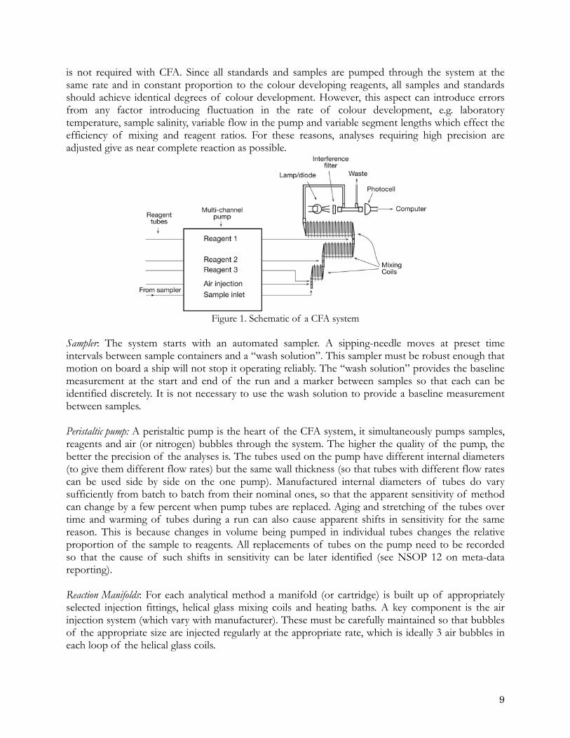
is not required with CFA. Since all standards and samples are pumped through the system at the same rate and in constant proportion to the colour developing reagents, all samples and standards should achieve identical degrees of colour development. However, this aspect can introduce errors from any factor introducing fluctuation in the rate of colour development, e.g. laboratory temperature, sample salinity, variable flow in the pump and variable segment lengths which effect the efficiency of mixing and reagent ratios. For these reasons, analyses requiring high precision are adjusted give as near complete reaction as possible.

Figure 1. Schematic of a CFA system

Sampler: The system starts with an automated sampler. A sipping-needle moves at preset time intervals between sample containers and a “wash solution”. This sampler must be robust enough that motion on board a ship will not stop it operating reliably. The “wash solution” provides the baseline measurement at the start and end of the run and a marker between samples so that each can be identified discretely. It is not necessary to use the wash solution to provide a baseline measurement between samples. Peristaltic pump: A peristaltic pump is the heart of the CFA system, it simultaneously pumps samples, reagents and air (or nitrogen) bubbles through the system. The higher the quality of the pump, the better the precision of the analyses is. The tubes used on the pump have different internal diameters (to give them different flow rates) but the same wall thickness (so that tubes with different flow rates can be used side by side on the one pump). Manufactured internal diameters of tubes do vary sufficiently from batch to batch from their nominal ones, so that the apparent sensitivity of method can change by a few percent when pump tubes are replaced. Aging and stretching of the tubes over time and warming of tubes during a run can also cause apparent shifts in sensitivity for the same reason. This is because changes in volume being pumped in individual tubes changes the relative proportion of the sample to reagents. All replacements of tubes on the pump need to be recorded so that the cause of such shifts in sensitivity can be later identified (see NSOP 12 on meta-data reporting). Reaction Manifolds: For each analytical method a manifold (or cartridge) is built up of appropriately selected injection fittings, helical glass mixing coils and heating baths. A key component is the air injection system (which vary with manufacturer). These must be carefully maintained so that bubbles of the appropriate size are injected regularly at the appropriate rate, which is ideally 3 air bubbles in each loop of the helical glass coils.

9

Colorimeter: From the manifold the reacted-coloured solution passes through the colorimeter. In a standard AA-II (Technicon) type system the light source is a filament bulb and the selection of analytical wavelength is achieved by passing the light through a suitable interference filter. In an AA-II type system a debubbler is used to remove the air bubbles before they can enter the detector cell. The individual segments begin to mix at this point. The detector cell is essentially a glass tube inline with the light source and the detector, which is a photo-diode (or photo-tube in newer systems). The solution is brought in and out of the light path by bends in the glass tube. This means that a detector cell is not optically perfect and some light path refractive distortion can occur (Froelich and Pilson, 1978; Dias et al., 2006). If the wash and sample are of different densities spurious signals can be generated at the beginning and end of each peak as light is refracted by the gradient formed as they mix. Newer systems tend to have better optics and in some cases the bubbles are allowed to pass through the flowcell. Noise from the bubble is either removed by gating the light source in time with the bubbles or by electronically processing the signal to detect and remove the bubble signals. 2.5.2 Assembly and maintenance For satisfactory results the components must be arranged with several ideas in mind. (1) The path lengths between sampler and pump, pump and manifold etc. must be minimised. This

is especially true of sections of the flow streams that are not segmented by air bubbles, e.g. the lines between the sampling needle and the pump. A long un-segmented stream can lead to excessive mixing between samples and wash water.

(2) Transmission tubing connected to reagent pump tubes should have a diameter similar to the

pump tube or up to 30% smaller. Transmission tubing carrying the bubble-segmented stream should have the same diameter as the glass manifold fittings or up to 30% less. This also applies to the waste line carrying bubbles from the colorimeter; a regular bubble pattern should be maintained throughout its length. As the diameter relative to the volume increases, resistance to pumping increases and surging can develop in the flow. This induces noise.

(3) All components should be arranged to avoid hydraulic pressure heads along the flow stream.

Hydraulic heads tend to generate surging in the flow. It is not good practice to locate reagent reservoirs on shelves over the CFA, or have drain tubes of small diameter, which go directly into receptacles on the floor.

(4) Avoid "dead volumes" in the flow channels. Dead volumes are usually introduced by de-bubblers

and gaps in the butt joints between glass fittings.

(5) A regular bubble pattern is essential for a noise-free output signal. Achieving good bubble patterns depends upon the system cleanliness and on ensuring that all plastic tubing through which bubbles pass, including the waste line from the detector, is wetted. Good bubbles appear round at the front and back, whereas in non-wetting conditions the bubbles appear straight at the back. At the end of each day’s operation the reagent and manifold line should be flushed with pure water followed by a phosphate free cleansing agent such as Decon 90, then by pure water again.

2.6 Preparation of reagents

10

2.6.1 Specifications of reagents Problems with reagents purity should be minimised by using “Analytical Grade” reagents. Due to the way a CFA system works small amounts of contamination can be tolerated, as they will produce a constant offset in the reagent baseline, which equally affects samples and standards equally. Reagent contamination is a problem when it produces sufficient absorbance to push the total absorbance into a nonlinear range. The reagent absorbance relative to water should be measured regularly. In general, the higher the reagent absorbance, the higher the detection limit of the method. When weighing and packaging "pre-weighed" solid reagents for work at sea, the label of each package should identify the batch of chemical from which the weighing was done. A corresponding record should be kept of the name of the manufacturer and lot number from the label of the original container. Good practice, when making up the reagent solutions, is to record when and from what source each batch of reagent was prepared and the time and date when its use was begun. Such information can be invaluable for tracing sources of problems arising from "bad batches" of reagents or improperly formulated or weighed reagents. 2.6.2 Reagent containers and their maintenance Containers should be convenient to use and easy to clean. The use of glass should be kept to minimum to avoid silica contamination by glass dissolution (Zhang et al., 1999). Tap water must never be used because of the high levels of Si and NO3 it usually contains. Use generous quantities of pure water for cleaning and Decon 90, if necessary. Once a container is clean – it should be kept clean by sealing it – simply put the lid back on – it does not need to be dry. In some laboratories atmospheric ammonium can cause contamination problems. Regular cleaning of storage containers reduces variance in the analytical results, as reagents degrade more slowly in well-maintained bottles than in dirty ones. When solutions are transferred all spillages on the outside of bottles should be cleaned off. The biggest danger resulting from poor cleanliness is that molybdenum blue stains on the necks of bottles are allowed to form. If this contamination gets into the reagent solution it will go blue through an auto-catalytic reaction. The acidified molybdate reagent used in the determination of Si throws a white precipitate as it ages. This is easily controlled at sea where the solution is replaced regularly by simply rinsing the molybdate solution bottles with pure water. If a precipitate does form in the bottle it can be dissolved with a solution of 10 % Decon 90 in pure water. 2.6.3 Pure Water Dependably pure water is a necessity for nutrient work. The use of distilled water should be avoided because it can be contaminated by Si (from glass stills) and N-compounds (ammonium and nitrogen oxides) absorbed from the atmosphere during its production. Water prepared by reverse osmosis followed by deionisation should be used where possible. Such systems are now commonly available on research ships. Ideally the water should be of 18 megohm.cm specific resistance. If possible pure water should not be stored because, as noted for distillation, ammonium and nitrogen oxides can be absorbed from the ships atmosphere. Similarly glass containers should be avoided due to Si contamination (Zhang et al, 1999). Note: Sonicating pure water to degas it can sonochemically produce measurable concentrations of nitrite from dissolved nitrogen gas. 2.6.4 Wash and blank solutions

11

All CFA systems tend to suffer from spurious signals when solutions of different density are present in the detector cell. Therefore a wash solution must have a matrix with similar optical density to that of the seawater samples being measured. The wash solution is also commonly used for the preparation of the calibration standards. In a CFA system a chemical reaction may not be complete when the coloured solution passes through the detector cell. The sample matrix can affect the rate of colour formation. The apparent sensitivity of the method could be different between standards and samples if the compositions of the wash solution and samples are significantly different. You MUST check if the methods you are using give different apparent sensitivities when standards made up in pure water, seawater or sodium chloride solution. 2.6.5 Choice of blank and wash solutions The ideal wash solution and matrix for preparation of calibration standards is natural seawater of similar salinity to the samples being measured and which contains undetectable or low concentrations of the analytes. Some laboratories are in the fortunate position of being able to collect, store and validate a large volume of natural seawater with low concentrations of nutrients. This water is then used at sea as both the wash solution and for the preparation of working standards. Such water should be collected and filtered through a filter having a pore size of 1 microns or smaller and then be stored in the dark for several months to stabilise. Before it is used the nutrient concentration in the aged water should be checked, ideally by a more sensitive method than the one that will be used for during the cruise. Sodium chloride solution containing 40 g l-1 has been used successfully as artificial seawater (ASW) wash and for the preparation of standards, as it has the same refractive index as seawater at salinity 35 and for most analyses the rates of the reaction are not significantly different from those in seawater. Whether LNS or ASW are used as the wash they are effectively taken to be the “zero” standard, therefore meticulous attention must be paid to monitoring the quality of these waters with respect to their nutrient content. Details of how this should be done are provided in NSOP 10. When ASW is prepared from sodium chloride each batch of sodium chloride needs to be checked. Although contamination with respect to PO4 and NO3 is rare it does occur, but more common is contamination by Si. This can be as large as a few µM kg-1 and requires the rejection of batches of sodium chloride. With the advent of newer instrumentation with better flowcell optics, a number of laboratories are using pure water as the baseline wash water (Aminot et al. 2009). It may be used for the sampler wash when the values recorded from it are not used in the calculation of the sample concentrations, because a separate “zero” standard of LNS or ASW is used. 2.7 Preparation of calibration standard solutions 2.7.1 Procedure for preparation of standard solutions CFA systems determine a concentration in terms of mass of determinand per volume of solution relative to a series of standard solutions. The concentration determined is therefore at the

12

temperature at which the standard solutions were prepared. It is this temperature that should to calculate the density of the sample, when converting from µM l-1 to µM kg-1. Primary (concentrated) standards are prepared using analytical-grade salts and ultra-pure water. Working standards are prepared in either nutrient-depleted natural seawater or artificial seawater. The accuracy of the preparation of the standard solution is critical. To achieve high quality measurements the salts must be dried and ground carefully before weighing. Salts should be dried in an oven at 105 °C for 2 hours then cooled in a desiccator. Higher temperatures should not used for drying to avoid decomposing the salts. If salts are not dried prior to weighing, errors of 2-3 % can arise. Weighing should take into account air buoyancy (NSOP 1). The primary and secondary standards should be made up and diluted into volumetric flasks whose volumes have been checked. Dilution of primary standards must be done using calibrated pipettes of known reliability (NSOP 2). Please note well: The use of un-calibrated plastic volumetric ware and lack of attention to solution temperature at the time of making up standards can lead to aggregate errors on the order of three percent or even greater.. 2.7.2 Volumetric Laboratory Ware (NSOP 1 & 2) To ensure the accuracy of calibrations all volumetric glass and plastic-ware need to be gravimetrically calibrated. You can do this better than the manufacturer will do. Temperature effects upon volumes contained by borosilicate glass volumetric ware are well documented and volumes at ship and shore laboratory temperatures can be computed (NSOP 2, Lembeck, 1974). You should make yourself aware of the likely errors that can result from changing laboratory temperatures. The weights obtained from the calibration weighing must be corrected for the density of water and air buoyancy. The gravimetrically calibrated volumes must be used in computing concentrations of standard solutions. Plastic (polypropylene) volumetric flasks must be gravimetrically calibrated within 2-3 oC of the temperature at which they will be used. Gordon et al (1993) reported that the volumes of plastic volumetric flasks calibrated in the OSU laboratory can be stable over several years' time. However, the volumes of all plastic volumetric flasks must be checked before each cruise. If they have been dried in an oven the volume can be permanently shifted by as much as 1 %. Because of the better stability of Pyrex compared to plastics with respect to thermal expansion and because of the slow attack by DIW, Pyrex is recommended for preparation of the concentrated “primary” calibration standard solution. Exposure time to the Pyrex should be kept to minimum. Gordon et al. (1993) reported that Pyrex volumetric flasks gave initial dissolution rates of 0.03 to 0.045 µM kg-1 silicate per minute into LNSW and no detectable dissolution into DIW.” Similarly, Zhang et al (1999) demonstrated that dissolution from glassware can introduce micromolar silicate within a few hours. The extent of dissolution depends upon contact time, salinity and pH of solution, and the size and shape of the containers.” Therefore, glass for the initial dissolution of primary standards and then transfer solution immediately into plastic (polycarbonate) containers that have a low transpiration rate for water. 2.7.3 Pipettes (NSOP 2)

13

Fixed volume pipettes should be used. Pipettes with adjustable volume are not recommended for use at sea as the precision of these pipettes would need to be checked each time their volume was changed and this cannot be done at sea. All pipettes should have nominal calibration tolerances of 0.1% or better. Each pipette must be gravimetrically calibrated in order to verify and improve upon this nominal tolerance. This should be done before and after each cruise. All persons preparing standards on the cruise should be trained in the use of pipettes. Their ability to obtain good precision with the pipettes should be checked by an exercise in which they do multiple pipetting and weighing of each aliquot pipetted. 2.8 Check list of sources of error

1. Impurity of salts used to prepare standards can be a major source of error. For example it was traditionally assumed sodium hexafluorosilicate was only 96 % pure (Strickland and Parsons 1972). Where possible new standards should be compared with old and with materials prepared by other labs. A number of errors can occur with the preparation and dilution of primary and secondary standards. These errors may in some cases be relatively small in themselves but can accumulate.

2. Weighing – the air buoyancy correction is 0.1 %. 3. Volumetrics - grade A glassware tolerances range from 0.16 % at 25 ml to 0.04 % at 1000ml.

User calibration can reduce this error to 0.01 %. 4. Volumetrics - plastic can permanently shrink if heated (in for example a drying oven). The

volume change can exceed 1%. 5. Change in volume of glassware with temperature – the volume of Pyrex volumetric flask

calibrated at 20 oC will reduce by 0.015 % if cooled to 5 oC 6. Change in volume of an aqueous solution with temperature - the volume of a solution will

increase by 0.2 % if warmed from 5 oC to 20 oC. 7. “Eppendorf ” type air displacement pipettes are commonly used. These have precision of

0.1% if used carefully. The accuracy expected to be about 0.1 % of the stated value when the pipette is new.

8. Pipetting cold solution in an air displacement pipette can cause an increase in the volume by 5 % if a pipette at 20 oC is used to take solution from a bottle stored in a refrigerator.

9. Errors can arise in the output from CFA systems from the potential errors in calibration listed above and also from mechanical performance of the system. These errors (considered below) are difficult to quantify but can be minimized by using appropriate procedures and careful attention to details. Some modern systems have software, which helps by checking the optical, thermal and hydraulic characteristics of the instrument before a run can be started.

10. It is important that the analyser should be run in a thermally stable environment and the analyzer should be fully “warmed up” before an analytical run is started.

11. A record should be kept of the baseline height and the absorbance produced by the top standard – as an indicator of possible changes in or contamination of reagent or wash water solutions.

12. The stability (noise) of the reagent baseline directly determines the detection limit. It should be measured and recorded regularly, so that shifts in performance can identified.

13. “Carryover” of one sample to the next can occur depending on the manifold and the

14

sampling rate. It can be measured and corrected for when modern software packages are used. However for best performance particularly when samples with highly varying concentration are being run (say a across the thermocline), the system should be adjusted to reduce carryover to a minimum, ideally <1% of the proceeding peak height.

14. When a CFA system is working well, the variation between duplicate measurements of peak heights should be <0.2 % of the full-scale range of the analysis.

15. If a linear calibration curve is used to calculate non-linear absorbance signals, significant errors in nutrient data can occur. This is particularly true in samples whose concentrations are outside the range of calibrant concentrations. It can also be significant in the mid-range (causing errors of ~ 3 %) see section 4.3.1.

16. Major problems can occur even with the new software systems supplied with most new CFA systems, if that software is used thoughtlessly. Visual checks of peak shape, the position of peak picking and the plausibility of results should always be carried out.

Table 1. Summary of errors listed above that are possible at different stages of a CFA based

analysis Source of Error % Weighing Impure standard salt 4 Wet standard salt 3 Buoyancy 0.1 Volumetrics Heat distorted plastic 1 Not checked grade A 0.16 User calibrated 0.01 Temperature change glass (15 oC) 0.015 Temperature change water (15 oC) 0.200 Pipette - "Eppendorf" type Precision 0.1 Accuracy 0.1 Temperature effect 15 oC on air volume 5 CFA Inherent precision 0.1 Carryover <0.5 Forcing a linear fit to non linear calibration data. 3 Reporting µM l-1 as µMkg-1 or visa-versa 3

The errors listed above are summarised in Table 1. From this table it is clear that using consistent batches of pure salts for the preparation of standards is important for achieving consistent results. These salts must be prepared in a consistent manner including their drying and grinding before they are weighed (see NSOP 3). The potential total errors possible from preparing working standards from primary and secondary standards stored in a refrigerator, which are cold when pipetted should be noted and avoided. The next largest potential error is when a linear fit is forced on non linear calibration data (see section 4.3.1). It is also imperative that data are clearly reported as µM l-1 (this is the unit they are measured in at the temperature at which the calibration standards were prepared) or fully worked up as µM kg-1 taking into account the salinity of the sample (and the calibration temperature). Finally all volumetric ware must be checked and calibrated particularly plastic volumetric flasks and air displacement pipettes.

15

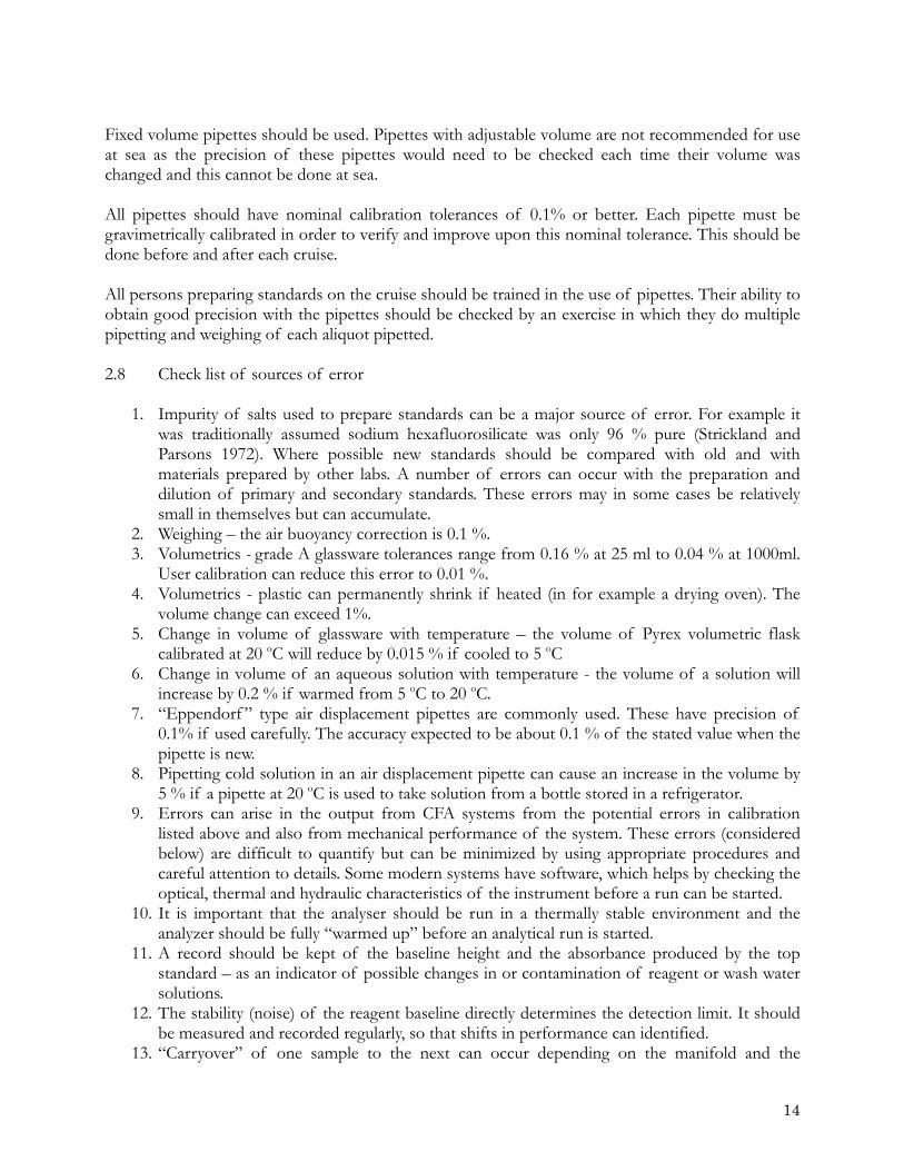
3. QUALITY ASSESSMENT 3.1 Precision and accuracy Precision is a measure of how reproducible a particular experimental procedure is. It can refer either to a particular stage of the procedure, e.g., the final analysis, or to the entire procedure including sampling and sample handling. It is quantified by performing replicate measurements and estimating a mean and standard deviation from the results. Accuracy is a measure of the degree of agreement of a measured value with the “true” value. An accurate method provides unbiased results. Quantification of accuracy is only possible when the “true” value is known. In practice this is possible when certified reference solutions can be measured as part of the everyday analytical procedure. 3.2 Quality assessment techniques A key part of any quality assurance program is the statistical evaluation of the quality of the data output. There are both internal and external techniques for quality assessment (see Taylor, 1987). Key internal techniques are duplicated measurements, internal test samples, control charts and audits. While external techniques include, collaborative tests, exchange of samples, external reference materials and audits. 3.3 Internal techniques 3.3.1 Duplicate measurements Duplicate measurements of an appropriate number of samples provide an evaluation of the precision that is being achieved. At least 10% of the samples should be measured in duplicate on each sample run. Differences between duplicates should be reported both as the true difference between the duplicates first minus the second value and the absolute difference. Ideally, one would analyse duplicate samples from all of the samples. Duplicates should be measured early and late in the run so that the difference measured gives an indication of drift in sensitivity occurring in the run and repeated as part of the next run to check for calibration differences between runs. A picture of variance during the cruise and for the whole cruise can then be built up, and recorded in the control charts for the cruise (NSOP 10). As an example nitrate concentration differences between duplicate measurements for 4600 pairs during the cruise R/V Mirai MR0706 and MR0704 cruises are shown below. In this case, about half of the duplicate measurements were within 0.2 % for the samples with concentrations between 35 – 40 µM kg-1 of nitrate.

16

0

500

1000

1500

2000

0 0.08 0.16 0.24 0.32 0.4 0.48 0.56 0.64 0.72 0.8

Num

ber o

f dat

a

micro mol kg-1

Figure 2. Nitrate concentration differences (absolute) between duplicate measurements of 4600 pairs during the cruise R/V Mirai MR0706 and MR0704 cruises. Nitrate concentrations were in the range between 35 µM

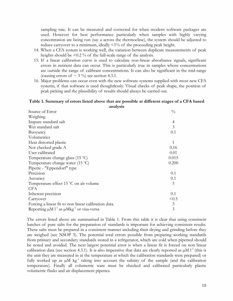
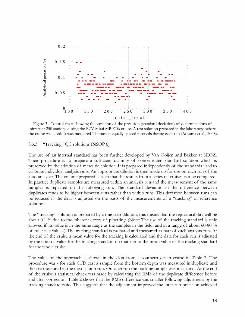
kg-1 and 40 µM kg-1. The width of the bar corresponds to 0.1% of the concentration of the samples. 3.3.2 Internal QC test solution An internal test solution prepared in a laboratory can be used to monitor precision and bias (drift between runs over the length of a cruise), if the test solution value can be prepared with sufficient precision. Similarly if the material (standard solution) used is sufficiently stable for a sufficiently long period of time it can also be used to assess bias between cruises. An example of the use of such an internal standard is shown below. This is control chart (See NSOP 10) for repeated measurements made on standard prepared in the laboratory before the cruise. At the end of cruise the information in these charts allows the work on the cruise to be evaluated. This ensures that the work is being carried out appropriately and that the necessary documentation is being maintained.

17

0

0 . 0 5

0 . 1

0 . 1 5

0 . 2

1 0 0 1 5 0 2 0 0 2 5 0 3 0 0 3 5 0 4 0 0

Ana

lytic

al p

reci

sion

/%

s t a t i o n _ s e r i a l Figure 3. Control chart showing the variation of the precision (standard deviation) of determinations of

nitrate at 250 stations during the R/V Mirai MR0706 cruise. A test solution prepared in the laboratory before the cruise was used. It was measured 11 times at equally spaced intervals during each run (Aoyama et al., 2008). 3.3.3 “Tracking” QC solutions (NSOP 6) The use of an internal standard has been further developed by Van Ooijen and Bakker at NIOZ. Their procedure is to prepare a sufficient quantity of concentrated standard solution which is preserved by the addition of mercuric chloride. It is prepared independently of the standards used to calibrate individual analysis runs. An appropriate dilution is then made up for use on each run of the auto-analyser. The volume prepared is such that the results from a series of cruises can be compared. In practice duplicate samples are measured within an analysis run and the measurement of the same samples is repeated on the following run. The standard deviation in the difference between duplicates tends to be higher between runs rather than within runs. This deviation between runs can be reduced if the data is adjusted on the basis of the measurements of a “tracking” or reference solution. The “tracking” solution is prepared by a one step dilution; this means that the reproducibility will be about 0.1 % due to the inherent errors of pipetting. (Note: The use of the tracking standard is only allowed if its value is in the same range as the samples in the field, and in a range of about 60-80 % of full scale values.) The tracking standard is prepared and measured as part of each analysis run. At the end of the cruise a mean value for the tracking is calculated and the data for each run is adjusted by the ratio of value for the tracking standard on that run to the mean value of the tracking standard for the whole cruise. The value of the approach is shown in the data from a southern ocean cruise in Table 2. The procedure was - for each CTD cast a sample from the bottom depth was measured in duplicate and then re-measured in the next station run. On each run the tracking sample was measured. At the end of the cruise a statistical check was made by calculating the RMS of the duplicate difference before and after correction. Table 2 shows that the RMS difference was smaller following adjustment by the tracking standard ratio. This suggests that the adjustment improved the inter-run precision achieved

18

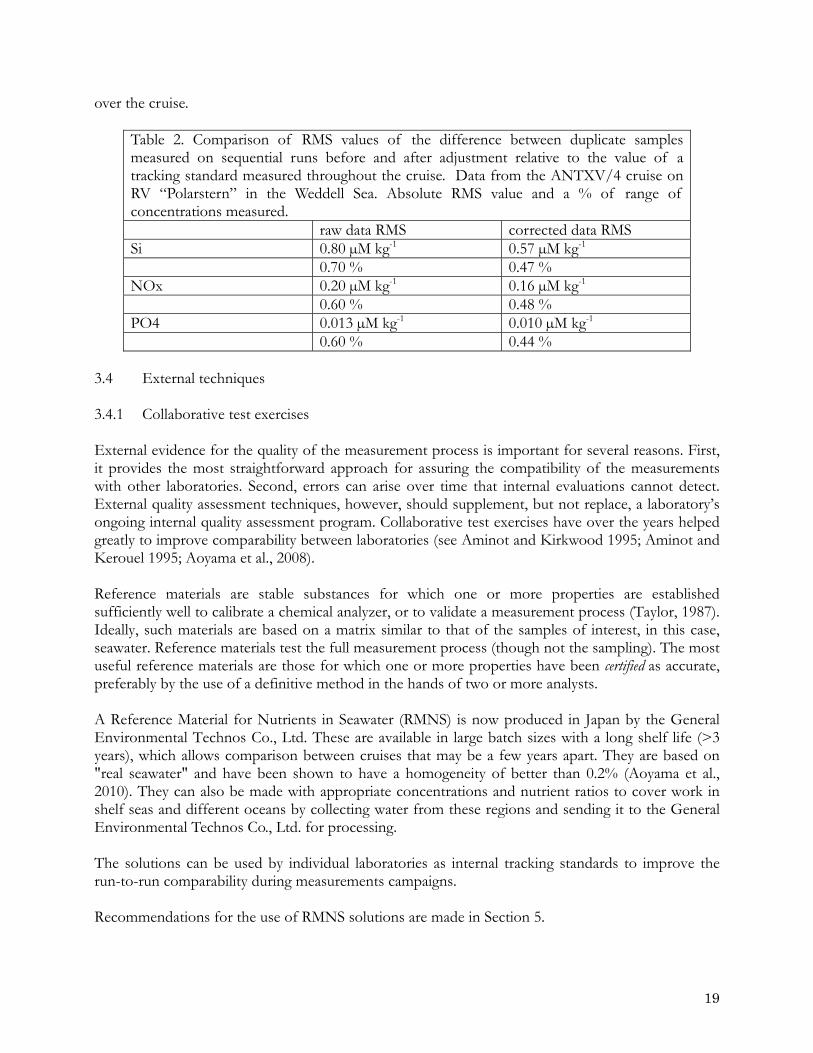
over the cruise.

Table 2. Comparison of RMS values of the difference between duplicate samples measured on sequential runs before and after adjustment relative to the value of a tracking standard measured throughout the cruise. Data from the ANTXV/4 cruise on RV “Polarstern” in the Weddell Sea. Absolute RMS value and a % of range of concentrations measured. raw data RMS corrected data RMS Si 0.80 µM kg-1 0.57 µM kg-1 0.70 % 0.47 % NOx 0.20 µM kg-1 0.16 µM kg-1 0.60 % 0.48 % PO4 0.013 µM kg-1 0.010 µM kg-1 0.60 % 0.44 %

3.4 External techniques 3.4.1 Collaborative test exercises External evidence for the quality of the measurement process is important for several reasons. First, it provides the most straightforward approach for assuring the compatibility of the measurements with other laboratories. Second, errors can arise over time that internal evaluations cannot detect. External quality assessment techniques, however, should supplement, but not replace, a laboratory’s ongoing internal quality assessment program. Collaborative test exercises have over the years helped greatly to improve comparability between laboratories (see Aminot and Kirkwood 1995; Aminot and Kerouel 1995; Aoyama et al., 2008). Reference materials are stable substances for which one or more properties are established sufficiently well to calibrate a chemical analyzer, or to validate a measurement process (Taylor, 1987). Ideally, such materials are based on a matrix similar to that of the samples of interest, in this case, seawater. Reference materials test the full measurement process (though not the sampling). The most useful reference materials are those for which one or more properties have been certified as accurate, preferably by the use of a definitive method in the hands of two or more analysts. A Reference Material for Nutrients in Seawater (RMNS) is now produced in Japan by the General Environmental Technos Co., Ltd. These are available in large batch sizes with a long shelf life (>3 years), which allows comparison between cruises that may be a few years apart. They are based on "real seawater" and have been shown to have a homogeneity of better than 0.2% (Aoyama et al., 2010). They can also be made with appropriate concentrations and nutrient ratios to cover work in shelf seas and different oceans by collecting water from these regions and sending it to the General Environmental Technos Co., Ltd. for processing. The solutions can be used by individual laboratories as internal tracking standards to improve the run-to-run comparability during measurements campaigns. Recommendations for the use of RMNS solutions are made in Section 5.

19

4. CALIBRATION PROCEDURES 4.1 Preparation of calibration solutions (NSOP 3) Working standard solutions for calibration of the analyser are prepared by serial dilution of primary standard solution. The primary standard solution is prepared at sea by dissolution of pure, crystalline standard materials, pre-weighed ashore. Preparation of the solutions is done using calibrated volumetric ware and pipettes (NSOP 2). Standard concentrations must be calculated for the exact masses taken, not the nominal weights. This includes correcting for air buoyancy (NSOP 1). The timing and frequency of preparation of standards should be consistent and carefully recorded. A complete and detailed record should be kept of all the identities of the pipettes, and volumetric flask used for preparation of each standard along with the label information for each pre-weighed standard used and the date and time of preparation of primary and secondary standards. It is expected that primary standard solutions of nitrate, phosphate and silicate should be stable for the duration of a normal hydrographic cruise lasting about a month. However to provide a check on the possible deterioration of the primary standards, new ones should be prepared every two weeks. The results from the "new" and "old" standards should be compared and used along with information from "tracking" standards to identify if deterioration of the primary standards has occurred. Serial dilution of the primary standards may require the preparation of an intermediate secondary standard. This will be prepared in pure water. It may be expected to be stable for several days if stored in a refrigerator, but it is best prepared daily. 4.2 Calibration of the nutrient analyzer 4.2.1 Overview Calibration of the analyser should be performed on each analytical run. This is necessary to take into accounts shifts in the sensitivity of the system due to changing conditions such as laboratory temperature, aging of pump tubes and degradation of the reagents. Calibration is normally carried out by:- (1) measuring a set of standards at the start of the run, (2) at regular intervals measuring the position of the baseline (3) repeatedly measuring a chosen solution- a “drift” standard (normally at 75 % of full scale) at regular intervals during the run to check for changes (drift) in sensitivity. The relative response of the system to nitrate relative to nitrite can change due to change in the efficiency of the cadmium column used to reduce nitrate to nitrite. A pair of standards one containing a high concentration of nitrate and the other an equivalent concentration of nitrite should be run and the results compared to assess the reduction efficiency of the cadmium column. If the efficiency is too low (<90%) or erratic the column should be replaced. To determine the amount of carryover from one sample to the next a high standard followed by two low ones should be run. The difference between the heights of the two low standards divided by the height of the high standard gives the carryover factor (Zhang, 1997). The concentration in each sample can then be calculated once the analytical run has been done and the data recorded. Modern CFA systems are now usually supplied with software that, based on a protocol, allows the

20

peaks to be detected and their height measured ignoring spikes in the data. The software links peaks to the types of samples and standards being measured at a given position in the run. It then calculates the concentration of nutrients in the samples taking into account the concentrations of standards, drifts, column efficiency and peak carryover. 4.2.2 Working standards The concentration of the working standards should cover the range expected in the sampled waters. Prior to cruise this can be found in historical data sets such as ocean atlases. The range to be used must be decided before a cruise and not changed between legs. A minimum of four working standards should be made up for each run. The range of concentrations should be evenly divided across the range of expected concentrations. 4.2.3 Linearity of calibrations (NSOP 4) In CFA work, systems are usually adjusted so that a near linear calibration can be used to compute sample concentrations. However, the linearity of method needs to be checked, particularly when working at high concentrations. With old instruments, small changes in flow volumes when changing tubes or changes in light source output can push a method response into the nonlinear range. Even with newer instruments we need to know the range of linearity for each method. The set up of the analyser should be adjusted by using an appropriate ratio of sample to reagents so that over the concentration ranges to be measured the analyser gives as close to linear response as possible. This should be checked to ensure the mid-scale offset from a straight line is <0.2%, use of a quadratic fit to the calibration data may be required to achieve this. 4.3 Linearity problems 4.3.1 Illustration of non-linearity based on data submitted to the INSS inter-comparison in 2008 For calibrating the data from a CFA system, if a laboratory bases its calibration on using only two known concentrations and a base line value then it can only derive a linear function, “y = ax + b” from the calibration data. If three or more levels of calibration solution are run then either a linear function or quadratic function (y = ax2 + bx + c) can be fitted to the calibration data. The choice should be based on experience of the output of the system. If a quadratic fit does give a better fit it should be checked to see if this is a true result or one generated by an error such the use of an inaccurate pipette. To check this a larger number (~10) of standards should run as samples and the raw peak heights examined (See NSOP 4). The 2008 Inter-laboratory comparison study provided an opportunity to assess the non-linear problem based on the results returned for the common RMNS solutions analysed. A number of the laboratories provided a description of their calibration procedures including the number of standards run and the type of fit (linear or quadratic) applied to the data. In Figure 4 the results reported by the different laboratories are compared as the difference between each laboratories results and the result determined by a laboratory that measured five calibration standards and then applied a quadratic fit to derive the calibration equation. The comparison is made for two different groups of laboratories. The first group (Group 1) of three laboratories measured five calibration standards and derived a calibration equation by a linear fit to the data. The second

21

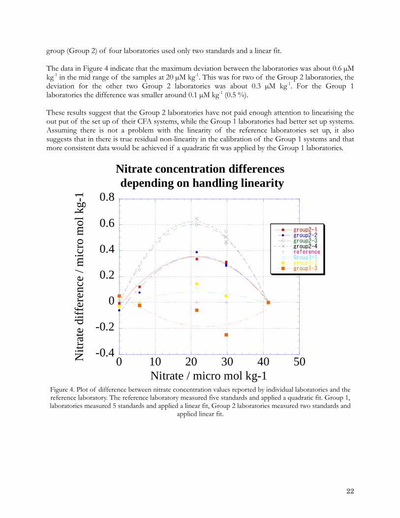
group (Group 2) of four laboratories used only two standards and a linear fit. The data in Figure 4 indicate that the maximum deviation between the laboratories was about 0.6 µM kg-1 in the mid range of the samples at 20 µM kg-1. This was for two of the Group 2 laboratories, the deviation for the other two Group 2 laboratories was about 0.3 µM kg-1. For the Group 1 laboratories the difference was smaller around 0.1 µM kg-1 (0.5 %). These results suggest that the Group 2 laboratories have not paid enough attention to linearising the out put of the set up of their CFA systems, while the Group 1 laboratories had better set up systems. Assuming there is not a problem with the linearity of the reference laboratories set up, it also suggests that in there is true residual non-linearity in the calibration of the Group 1 systems and that more consistent data would be achieved if a quadratic fit was applied by the Group 1 laboratories.

-0.4

-0.2

0

0.2

0.4

0.6

0.8

0 10 20 30 40 50

Nitrate concentration differences depending on handling linearity

group2-1group2-2group2-3group2-4referenceGroup1-1group1-2group1-3

Nitr

ate

diff

eren

ce /

mic

ro m

ol k

g-1

Nitrate / micro mol kg-1

Figure 4. Plot of difference between nitrate concentration values reported by individual laboratories and the reference laboratory. The reference laboratory measured five standards and applied a quadratic fit. Group 1, laboratories measured 5 standards and applied a linear fit, Group 2 laboratories measured two standards and

applied linear fit.

22

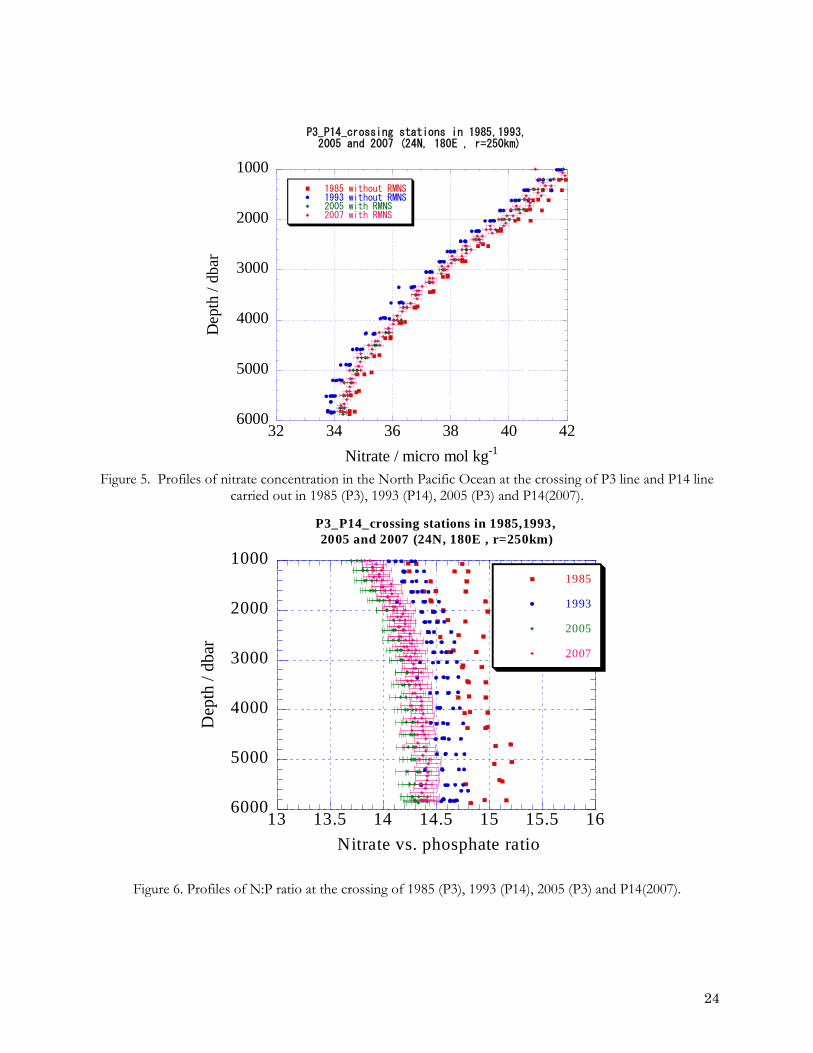
5. EXPERIENCE WITH USE OF RMNS SOLUTIONS The purpose of RMNS solutions is to improve the consistency of measurements within a cruise and between cruises. They are limited resource so need to be used in conjunction with internal standard solutions produced by each laboratory. The relative accuracy of in house standard solutions can then be validated when the RMNS values from a cruise are compared the values reported by other laboratories who have used the same batch of RMNS solutions. RMNS solutions are potentially more homogeneous than “tracking solutions” prepared from dry salts (see section 3.3.3 and NSOP 6). They should be used either in place of or alongside a laboratory’s internally prepared tracking solution. RMNS samples would be measured on each analytical run and the data would be used at the end of the cruise to adjust the data for the cruise in the same manner as is done when a tracking standard is used (NSOP 6). In the cruise meta-data all the RMNS values should be reported along with the mean, median and standard deviation. Inter-comparison exercises have shown evidence that discrepancies arise between different laboratories if inappropriate assumptions are being made about the linearity of calibration data. (See section 4.2.3 above). So that such non-linearity can be detected, a minimum of three RMNS solution at low, mid and top of the range should analysed at regular intervals during a cruise. Reporting these data in the meta-data at the end of cruise will allow non linearity to be identified when comparisons are made to the data reported by other laboratories who have measured the same RMNS solutions. 5.1 Example of improvement of comparability based on the use of RMNS solutions Figure 5 shows concentrations of nitrate in the North Pacific Ocean at the crossing point of four WOCE cruises for the WOCE lines P3 line and P14 (within 250 km of 24 oN - 180 oE). These were in 1985 (P3), 1993 (P14), 2005 (P3) and 2007 (P14). During the P3 cruise in 1985 and P14 cruise in1993, nutrients measurements were done using an in-house calibration standard. During the P3 and P14 reoccupation cruises in 2005 and 2007, a set of RMNS were used as calibration standard throughout the cruises. Figure 5.1 shows a much closer agreement between reoccupation cruise than between the earlier P3 and P14 cruises. Figure 6 shows that the use of the RMNS solutions produces data with tighter N:P ratio but also significant shift in the value of the ratio, from 15 to less than 14.5 at depth of 5000 metres.

23

32 34 36 38 40 42

1000

2000

3000

4000

5000

6000

P3_P14_crossing stations in 1985,1993, 2005 and 2007 (24N, 180E , r=250km)

1985 without RMNS1993 without RMNS2005 with RMNS2007 with RMNS

Nitrate / micro mol kg-1

Dep

th /

dbar

Figure 5. Profiles of nitrate concentration in the North Pacific Ocean at the crossing of P3 line and P14 line

carried out in 1985 (P3), 1993 (P14), 2005 (P3) and P14(2007). Figure 5.2 Profiles of N:P ratio at the crossing of 1985 (P3), 1993 (P14), 2005 (P3) and

13 13.5 14 14.5 15 15.5 16

1000

2000

3000

4000

5000

6000

P3_P14_crossing stations in 1985,1993, 2005 and 2007 (24N, 180E , r=250km)

1985

1993

2005

2007

Nitrate vs. phosphate ratio

Dep

th /

dbar

Figure 6. Profiles of N:P ratio at the crossing of 1985 (P3), 1993 (P14), 2005 (P3) and P14(2007).

24

6. NUTRIENT ANALYSIS DATA AND META-DATA REPORTING

(See NSOP 12 - Meta-data reporting) 6.1 Check list for reporting nutrient data Adequate and accurate records must be kept of all the procedures used and the results of the quality assessments of each reported data set: All archived data should be reported with this “meta-data” attached in electronic format. Without the meta-data to document methods and QA/QC protocols, archived data are of limited use. The material to be archived should include Samples results:

• Header file showing what was measured (variables/parameters, units) • Time and location of sample taken(time; latitude; longitude; station identifier) • Time the sample was measured • Raw nutrient data • Nutrient data adjusted for tracking and RMNS results • Clear statement that the data are reported as µM l-1 or µM kg-1

Quality control results:

• Control charts • Precision from duplicates in and between runs • Tracking solution data • RMNS data • Record of calculations and adjustments

Meta-Data on how the measurements were carried out:

• How the measurements were made (equipment, calibration, methodology etc., with references to literature, if available);

• Who measured it (name and institution of the analyst(s) and Principal Investigator responsible for the data);

• Quality assurance report • Data records

7. REFERENCES Aminot, A. and D. S. Kirkwood. 1995. Report on the results of the fifth ICES Inter-comparison study for

Nutrients in Seawater. ICES Cooperative Research Report No. 213, 79 pp. Aminot, A. and R. Kerouel. 1995. Reference material for nutrients in seawater: stability of nitrate,

nitrite, ammonium and phosphate in autoclaved samples. Mar. Chem. 49, 221–232. Aminot, A. and R. Kerouel. 2007. Dosage automatique des nutriments dans les eaux marines

methodes en flux continu. 188p. In Methodes d’analyse en milieu marin. Ifremer, ed. Editions

25

Quae ISBN 978-2-7592-0023-8. Aminot, A., R. Kerouel and S Coverly. 2009. Nutrients in Seawater Using Segmented Flow Analysis.

Pp. 143-178, Chapter 8 in Practical Guidelines for the Analysis of Seawater. Oliver Wurl, ed. CRC 2009 408pp ISBN-13: 978-1420073065.

Aoyama, M., J. Hamanaka, A. Kudo, Y. Otsubo, K.Sato, A. Yasuda, and S. Yokogawa. 2005. Nutrients,

Pp. 57-73 in WHP P6, A10, I3/I4 Revisit Data Book - Blue Earth Global Expedition 2003 (BEAGLE2003) – Volume 2, Hiroshi Uchida and Masao Fukasawa, eds., JAMSTEC, Yokosuka.

Aoyama, M., S. Becker, M. Dai, H. Daimon, L. I. Gordon, H. Kasai, R. Kerouel, N. Kress, D. Masten,

A. Murata, N. Nagai, H. Ogawa, H. Ota, H. Saito, K. Saito, T. Shimizu, H. Takano, A. Tsuda, K. Yokouchi and A. Youenou. 2007. Recent comparability of Oceanographic Nutrients Data: Results of a 2003 Intercomparison Exercise using Reference Materials. Analytical Science 23, 1151-1154.

Aoyama, M., J. Barwell-Clarke, S. Becker, M. Blum, Braga E. S., S. C. Coverly, E. Czobik, I. Dahllof,

M. H. Dai, G. O. Donnell, C. Engelke, G. C. Gong, Gi-Hoon Hong, D. J. Hydes, M. M. Jin, H. Kasai, R. Kerouel, Y. Kiyomono, M. Knockaert, N. Kress, K. A. Krogslund, M. Kumagai, S. Leterme, Yarong Li, S. Masuda, T. Miyao, T. Moutin, A. Murata, N. Nagai, G. Nausch, M. K. Ngirchechol, A. Nybakk, H. Ogawa, J. van Ooijen, H. Ota, J. M. Pan, C. Payne, O. Pierre-Duplessix, M. Pujo-Pay, T. Raabe, K. Saito, K. Sato, C. Schmidt, M. Schuett, T. M. Shammon, J. Sun, T. Tanhua, L. White, E.M.S. Woodward, P. Worsfold, P. Yeats, T. Yoshimura, A.Youenou and J. Z. Zhang. 2008. 2006 Inter-laboratory Comparison Study of a Reference Material for Nutrients in Seawater. Technical Reports of the Meteorological Research Institute 58, 104 pp., Tsukuba, Japan.

Aoyama, M. C.and co-authors. 2010. 2008 Inter-laboratory Comparison Study of a Reference

Material for Nutrients in Seawater. Technical Reports of the Meteorological Research Institute 60, 134 pp., Tsukuba, Japan.

Atlas, E. L., S. W. Hager, L. I. Gordon and P. K. Park. 1971. A practical manual for use of the Technicon

Autoanalyser in seawater nutrient analyses; Revised. Technical Report 215. Oregon State University, Dept of Oceanography, Ref. No. 71-22. 48 pp.

Dias A.C., E.P. Borges, E.A. Zagatto, and P.J. Worsfold. 2006. A critical examination of the

components of the Schlieren effect in flow analysis. Talanta 68,1076-1082. Dickson, A.G., C.L. Sabine, and J.R. Christian, eds. 2007. Guide to best practices for ocean CO2

measurements. PICES Special Publication 3, 191 pp. Dux, J.P., (1990). Handbook of Quality Assurance for the Analytical Chemistry Laboratory, 2nd edn.

Van Nostrand Reinhold, New York, 203 pp. Froelich P.N. and M.E.Q. Pilson 1978. Systematic absorbance errors with Technicon Autoanalyser II

colorimeters. Water Res. 12, 599-603.

26

Gordon, L.I., J.C. Jennings, A.A. Ross, and J.M. Krest. 1993. A Suggested Protocol for Continuous Flow Automated Analysis of Seawater Nutrients (Phosphate, Nitrate, Nitrite and Silicic Acid). In The WOCE Hydrographic Program and the Joint Global Ocean Fluxes Study , WOCE Hydrographic Program Office, Methods Manual WHPO 91-1.

Gouretski V.V. and K. Jancke. 2001. Systematic errors as the cause for an apparent deep water

property variability: global analysis of the WOCE and historical hydrographic data. Progress in Oceanography 48, 337–402.

Lembeck, J. 1974. The Calibration of Small Volumetric Laboratory Glassware. NBSIR 74-461. Available

online at: http://ts.nist.gov/MeasurementServices/Calibrations/upload/74-461.PDF. MacDonald, R.W., F.A. McLaughlin and C.S. Wong. 1986. Storage of reactive silicate samples by

freezing. Limnol.Oceanogr. 31: 1139-1142. Mee, L.D. 1986. Continuous flow analysis in chemical oceanography: Principles, applications and

perspectives. Sci. Total Environ. 49, 27-87. Mostert, S.A.. 1988. Notes on improvements and modifications to the automatic methods for

determining dissolved micronutrients in seawater. S. Afr. J. Mar. Sci. 7, 295-298. Olafsson, J. and A. Olsen. 2010. Nordic Seas nutrients data in CARINA. Earth Syst. Sci. Data Discuss.,

3, 55-78. Skeggs L.T. Jr. 2000. Persistence and Prayer: From the Artificial Kidney to the AutoAnalyzer. Clinical

Chemistry 46, 1425-1436. Strickland, J.D.H. and T.R. Parsons. 1972. A practical handbook of sea-water analysis (2nd Edition). J.

Fish. Res. Bd. Canada. 167, 311 pp. Tanhua, T., P. J. Brown, and R. M. Key. 2009. CARINA: nutrient data in the Atlantic Ocean. Earth

Syst. Sci. Data 1, 7-24. Taylor, J.K. and H.V. Oppermann. 1986. Handbook for the quality assurance of metrological measurements.

National Bureau of Standards. NBS Handbook 145. Vijverberg F. A. J. M. and W. P. Cofino. 1987. Control procedures: good laboratory practice and quality

assurance. ICES Techniques in Marine Science No. 6. Zhang, J.-Z. 1997. Distinction and quantification of carryover and sample interaction in gas

segmented continuous flow analysis. Journal of Automatic Chemistry Vol. 19, No.6, 205-212. Zhang, J.-Z. and P. B. Ortner. 1998. Effect of thawing conditions on the recovery of reactive silicic

acid from frozen natural water samples. Water Research 32, 2553-2555. Zhang, J.-Z., C. Fischer and P. B. Ortner. 1999. Dissolution of silicate from glassware as a

contaminant in silicate analysis of natural water samples. Water Research 33, 2879-2883.

27

28

8. ACKNOWLEDGEMENTS In November 2007 Michio Aoyama of the Japanese Meteorological Research Institute organised a meeting in Tsukuba, Japan to discuss the establishment of an “International Scale for the Measurements of Nutrients in Seawater” (INSS) as part of a process that would improve the international comparability of nutrient measurements in seawater. This would be based on the development of seawater based reference solutions which could then be used by all laboratories making measurements of nutrients in seawater. The meeting also recognised that progress towards a higher level of intercomparability would be hindered if best practice were not followed by the laboratories using these new reference seawater materials. The meeting therefore agreed to work on an update of the Gordon et al (1993) protocols developed to support the WOCE hydrographic programme. The aim was to explain and illustrate best practice, taking as their starting point as the excellent work of Lou Gordon and the team he led to prepare “A Suggested Protocol for Continuous Flow Automated Analysis of Seawater Nutrients (Phosphate, Nitrate, Nitrite and Silicic Acid) in the WOCE Hydrographic Program and the Joint Global Ocean Fluxes Study by Louis I. Gordon, Joe C. Jennings, Jr. Andrew A. Ross, James M. Krest (1993) WOCE Hydrographic Program Office, Methods Manual WHPO 91-1”. The format of the new document follows that of Dickson et al. (2007) [Dickson, A.G., Sabine, C.L. and Christian, J.R. (Eds.) 2007. Guide to best practices for ocean CO2 measurements. PICES Special Publication 3, 191 pp.] in having a central text accompanied by a set of individual standard operating procedures (SOPs). The content of several of our nutrient standard operating procedures (NSOPs) follows very closely the content of ones of Dickson et al. Andrew Dickson very kindly supplied the original “Word” files for the carbonate SOPs for use in preparing the NSOPs.

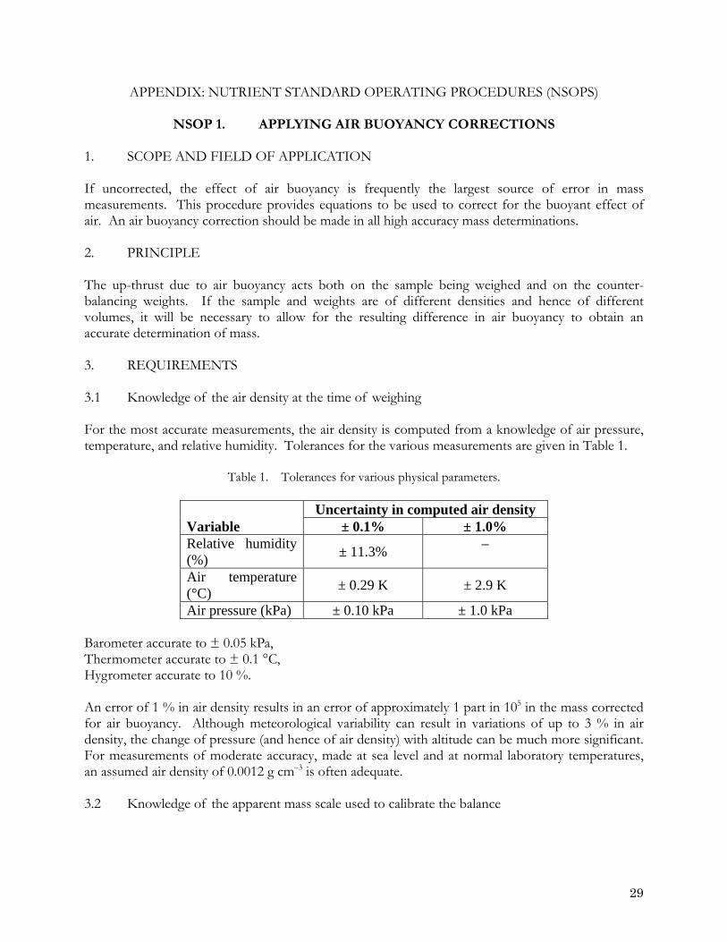
APPENDIX: NUTRIENT STANDARD OPERATING PROCEDURES (NSOPS)

NSOP 1. APPLYING AIR BUOYANCY CORRECTIONS 1. SCOPE AND FIELD OF APPLICATION If uncorrected, the effect of air buoyancy is frequently the largest source of error in mass measurements. This procedure provides equations to be used to correct for the buoyant effect of air. An air buoyancy correction should be made in all high accuracy mass determinations. 2. PRINCIPLE The up-thrust due to air buoyancy acts both on the sample being weighed and on the counter-balancing weights. If the sample and weights are of different densities and hence of different volumes, it will be necessary to allow for the resulting difference in air buoyancy to obtain an accurate determination of mass. 3. REQUIREMENTS 3.1 Knowledge of the air density at the time of weighing For the most accurate measurements, the air density is computed from a knowledge of air pressure, temperature, and relative humidity. Tolerances for the various measurements are given in Table 1.

Table 1. Tolerances for various physical parameters.

Variable Uncertainty in computed air density

± 0.1% ± 1.0% Relative humidity (%) ± 11.3% –

Air temperature (°C) ± 0.29 K ± 2.9 K

Air pressure (kPa) ± 0.10 kPa ± 1.0 kPa Barometer accurate to ± 0.05 kPa, Thermometer accurate to ± 0.1 °C, Hygrometer accurate to 10 %. An error of 1 % in air density results in an error of approximately 1 part in 105 in the mass corrected for air buoyancy. Although meteorological variability can result in variations of up to 3 % in air density, the change of pressure (and hence of air density) with altitude can be much more significant. For measurements of moderate accuracy, made at sea level and at normal laboratory temperatures, an assumed air density of 0.0012 g cm–3 is often adequate. 3.2 Knowledge of the apparent mass scale used to calibrate the balance

29

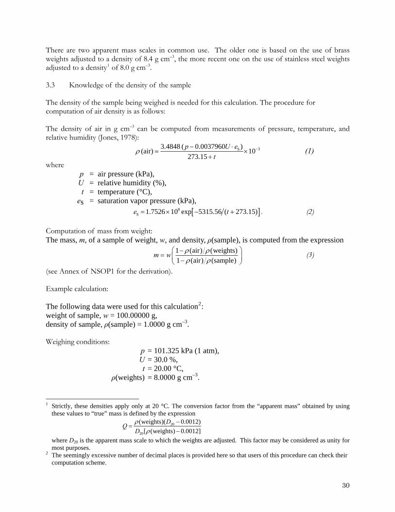
There are two apparent mass scales in common use. The older one is based on the use of brass weights adjusted to a density of 8.4 g cm–3, the more recent one on the use of stainless steel weights adjusted to a density1 of 8.0 g cm–3. 3.3 Knowledge of the density of the sample The density of the sample being weighed is needed for this calculation. The procedure for computation of air density is as follows: The density of air in g cm–3 can be computed from measurements of pressure, temperature, and relative humidity (Jones, 1978):

3S3.4848 ( 0.0037960 )(air) 10273.15

p U et

ρ −− ⋅=

+× (1)

where p = air pressure (kPa), U = relative humidity (%), t = temperature (°C), es = saturation vapor pressure (kPa),

[ ]8S 1.7526 10 exp 5315.56 ( 273.15)e t= × − + . (2)

Computation of mass from weight: The mass, m, of a sample of weight, w, and density, ρ(sample), is computed from the expression

1 (air) (weights)1 (air) (sample)

m w ρ ρρ ρ

⎛ −= ⎜ −⎝ ⎠

⎞⎟

(3)

(see Annex of NSOP1 for the derivation). Example calculation: The following data were used for this calculation2: weight of sample, w = 100.00000 g, density of sample, ρ(sample) = 1.0000 g cm–3. Weighing conditions: p = 101.325 kPa (1 atm), U = 30.0 %, t = 20.00 °C, ρ(weights) = 8.0000 g cm–3.

1 Strictly, these densities apply only at 20 °C. The conversion factor from the “apparent mass” obtained by using

these values to “true” mass is defined by the expression

20

20

(weights)( 0.0012)[ (weights) 0.0012]

DQ

Dρ

ρ−

=−

where D20 is the apparent mass scale to which the weights are adjusted. This factor may be considered as unity for most purposes.

2 The seemingly excessive number of decimal places is provided here so that users of this procedure can check their computation scheme.

30

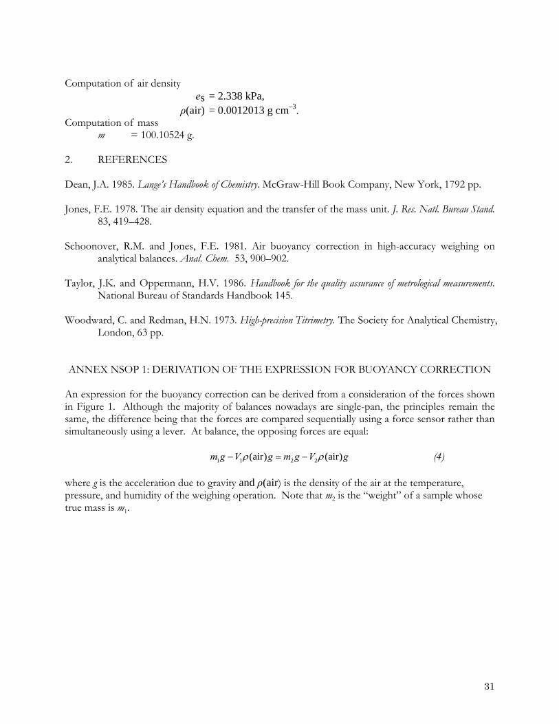
Computation of air density es = 2.338 kPa, ρ(air) = 0.0012013 g cm–3. Computation of mass m = 100.10524 g. 2. REFERENCES Dean, J.A. 1985. Lange’s Handbook of Chemistry. McGraw-Hill Book Company, New York, 1792 pp. Jones, F.E. 1978. The air density equation and the transfer of the mass unit. J. Res. Natl. Bureau Stand.

83, 419–428. Schoonover, R.M. and Jones, F.E. 1981. Air buoyancy correction in high-accuracy weighing on

analytical balances. Anal. Chem. 53, 900–902. Taylor, J.K. and Oppermann, H.V. 1986. Handbook for the quality assurance of metrological measurements.

National Bureau of Standards Handbook 145. Woodward, C. and Redman, H.N. 1973. High-precision Titrimetry. The Society for Analytical Chemistry,

London, 63 pp. ANNEX NSOP 1: DERIVATION OF THE EXPRESSION FOR BUOYANCY CORRECTION

An expression for the buoyancy correction can be derived from a consideration of the forces shown in Figure 1. Although the majority of balances nowadays are single-pan, the principles remain the same, the difference being that the forces are compared sequentially using a force sensor rather than simultaneously using a lever. At balance, the opposing forces are equal:

1 1 2 2(air) (air)m g V g m g V gρ ρ− = − (4) where g is the acceleration due to gravity and ρ(air) is the density of the air at the temperature, pressure, and humidity of the weighing operation. Note that m2 is the “weight” of a sample whose true mass is m1.

31

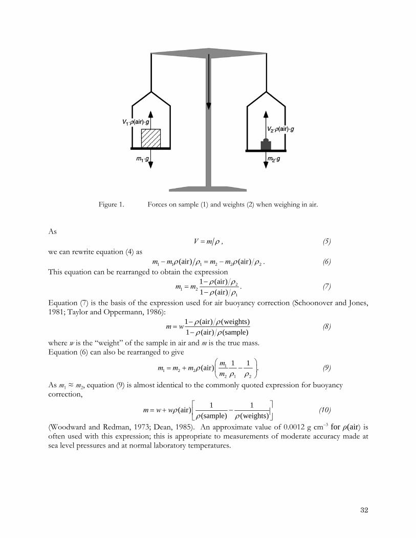
Figure 1. Forces on sample (1) and weights (2) when weighing in air. As

V m ρ= , (5) we can rewrite equation (4) as

1 1 1 2 2(air) (air)m m m m 2ρ ρ ρ− = − ρ . (6) This equation can be rearranged to obtain the expression

21 2

1

1 (air)1 (air)

m m ρ ρρ ρ

−=

−. (7)

Equation (7) is the basis of the expression used for air buoyancy correction (Schoonover and Jones, 1981; Taylor and Oppermann, 1986):

1 (air) (weights)1 (air) (sample)

m w ρ ρρ ρ

−=

− (8)

where w is the “weight” of the sample in air and m is the true mass. Equation (6) can also be rearranged to give

11 2 2

2 1 2

1 1(air) .mm m mm

ρρ ρ

⎛ ⎞= + −⎜

⎝ ⎠⎟ (9)

As m1 ≈ m2, equation (9) is almost identical to the commonly quoted expression for buoyancy correction,

1 1(air)(sample) (weights)

m w wρρ ρ⎡ ⎤

= + −⎢ ⎥⎣ ⎦

(10)

(Woodward and Redman, 1973; Dean, 1985). An approximate value of 0.0012 g cm–3 for ρ(air) is often used with this expression; this is appropriate to measurements of moderate accuracy made at sea level pressures and at normal laboratory temperatures.

32

NSOP 2. GRAVIMETRIC CALIBRATION OF VOLUME CONTAINED IN VOLUMETRIC FLASKS AND PIPETTES USING WATER

1. SCOPE AND FIELD OF APPLICATION This procedure describes how to calibrate the volume of solution contained by volumetric flasks, pipettes or other containers capable of being filled to a reproducible mark. This is expressed as the volume contained at a standard temperature (usually 20.0°C). This procedure is capable of achieving a reproducibility of better than 0.01% (1 relative standard deviation). “Eppendorf ” type air displacement pipettes are commonly used along with volumetric flasks for the preparation of calibration solutions. These have precision of 0.1 % if used carefully. The accuracy expected to be about 0.1 % of the stated value when the pipette is new. Their precision and accuracy should be checked on a regular basis. 2. PRINCIPLE The mass of water contained by the flask at a measured calibration temperature is used to compute the volume of water contained at that temperature. The volume that would be contained at the standard temperature (20°C) can be calculated by taking account of the volumetric expansion of the flask. The volume of liquid contained at any desired temperature can be calculated in a similar fashion. Warning. This requires that the temperature of the calibration solution is known. Taking solutions directly from a refrigerator and preparing a standard solution should be avoided for this reason. Similarly pipetting cold solution in an air displacement pipette can cause an increase in the volume by 5 % if a pipette calibrated at 20oC is used to pipette a solution at 5oC. This because the cold solution once in the pipette can cause the air above it to contract. 3. APPARATUS

• Analytical balance capable of weighing the quantity of water contained with a sensitivity of 1 part in 105 while having the capacity to weigh the water together with the container being calibrated.

• Thermometer accurate to ± 0.1 °C. • Container large enough to retain more than 10 aliquots dispensed by the pipette being

calibrated. 4. REAGENTS

• Deionised water in equilibrium with the temperature of the laboratory. 5. PROCEDURE CALIBRATION OF VOLUMETRIC FLASKS

• Weigh the clean dry empty container together with the associated closure. • Fill the container being calibrated to the mark with pure water, allowing the temperature

of the container and contained water to reach an equilibrium value. Note this temperature.

33

• Close the container and reweigh it.

6. CALCULATION AND EXPRESSION OF RESULTS 6.1 Volume of the water contained at the calibration temperature Compute the weight of the water contained from the difference between weights of the filled and empty container: . (11) 2

Compute the mass of water contained, correcting for air buoyancy (see NSOP 1): (H O) (filled container) (empty container)w w w= −

2 21 (air) (weights)(H O) (H O) .1 (air) (sample)

m w ρ ρρ ρ

⎛ ⎞−= ⎜ ⎟−⎝ ⎠

(12)

The volume contained at the noted temperature (t) is 2 2( ) (H O) (H O, ) .V t m tρ= (13) The density of air-saturated water in the temperature range 5 to 40 °C is given by the expression (Jones and Harris, 1992)

3 2W

3 2 5

7 4

(kg m ) 999.84847 6.337563 10 ( / C)8.523829 10 ( / C) 6.943248 10 ( / C)3.821216 10 ( / C)

tt tt

ρ − −

− −

−

= + × °

− × ° + × °− × °

3

l

(14) where t is the temperature on ITS 903. To achieve an accuracy of 1 part in 104, t must be known to within 0.5 °C. 6.2 Volume that would be contained at an alternate temperature To convert the volume contained at one temperature (t1) to a standard or alternate temperature (t2), we need to take account of the thermal expansion of the container being used. For Pyrex-like glasses (Corning 7740, Kimble KG-33, Schott Duran, Wheaton 200, etc.) the coefficient of linear expansion αl is 32.5 × 10–7 K–1; for glasses such as Kimble KG-35, αl is about 55 × 10–7 K–1. The coefficient of volumetric expansion, 3(1 ) 1 3V lα α α= + − ≈ , (15) is used to calculate the corrected volume at the alternate temperature, . (16) [ ]2 1 2 1( ) ( ) 1 ( )VV t V t t tα= + −This correction is negligible for all except the most precise work; unless t2 – t1 exceeds 10 °C or if plastic ware is used. Example calculation: The following data were used for this calculation:

3 The International Practical Temperature Scale of 1968 (IPTS 68) has been superceded by the International

Temperature Scale of 1990 (ITS 90). A simple equation can be used to relate the two over the oceanographic temperature range 0 to 40 °C (Jones and Harris, 1992):

t90 = 0.0002 + 0.99975 t68. The small difference in temperature scales is typically not important to the calibration of glassware for the

procedures in this Guide.

34

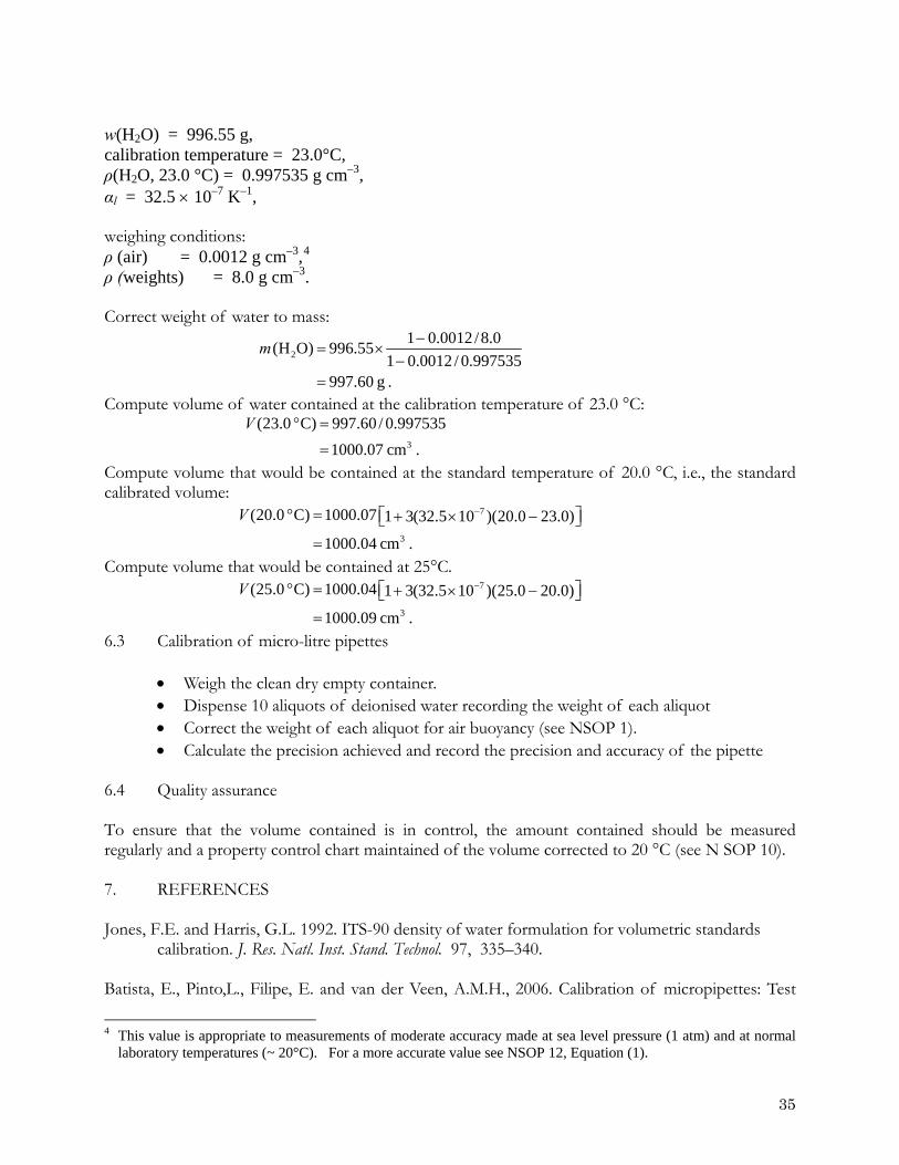
w(H2O) = 996.55 g, calibration temperature = 23.0°C, ρ(H2O, 23.0 °C) = 0.997535 g cm–3, αl = 32.5 × 10–7 K–1, weighing conditions: ρ (air) = 0.0012 g cm–3,4 ρ (weights) = 8.0 g cm–3. Correct weight of water to mass:

21 0.0012 /8.0(H O) 996.55

1 0.0012 / 0.997535997.60 g .

m −= ×

−=

Compute volume of water contained at the calibration temperature of 23.0 °C:

3

(23.0 C) 997.60 / 0.9975351000.07 cm .

V ° =

=Compute volume that would be contained at the standard temperature of 20.0 °C, i.e., the standard calibrated volume:

7

3

(20.0 C) 1000.07 1 3(32.5 10 )(20.0 23.0)

1000.04 cm .

V −° = ⎡ ⎤+ × −⎣ ⎦=

Compute volume that would be contained at 25°C.

7

3

(25.0 C) 1000.04 1 3(32.5 10 )(25.0 20.0)

1000.09 cm .

V −° = ⎡ ⎤+ × −⎣ ⎦=

6.3 Calibration of micro-litre pipettes

• Weigh the clean dry empty container. • Dispense 10 aliquots of deionised water recording the weight of each aliquot • Correct the weight of each aliquot for air buoyancy (see NSOP 1). • Calculate the precision achieved and record the precision and accuracy of the pipette

6.4 Quality assurance To ensure that the volume contained is in control, the amount contained should be measured regularly and a property control chart maintained of the volume corrected to 20 °C (see N SOP 10). 7. REFERENCES Jones, F.E. and Harris, G.L. 1992. ITS-90 density of water formulation for volumetric standards

calibration. J. Res. Natl. Inst. Stand. Technol. 97, 335–340. Batista, E., Pinto,L., Filipe, E. and van der Veen, A.M.H., 2006. Calibration of micropipettes: Test

4 This value is appropriate to measurements of moderate accuracy made at sea level pressure (1 atm) and at normal

laboratory temperatures (~ 20°C). For a more accurate value see NSOP 12, Equation (1).

35

methods and uncertainty analysis. Measurement 40, 338-342. doi:10.1016/j.measurement.2006.05.01.

36

NSOP 3. PREPARATION OF CALIBRATION SOLUTIONS FOR USE WITH CFA SYSTEM

1. SCOPE AND FIELD OF APPLICATION This NSOP describes the preparation of the solutions needed to calibrate a segmented continuous flow analyser (CFA) used to determine dissolved nutrients - ammonium, nitrate, nitrite, phosphate and silicate. 2. PRINCIPLE Primary standard solutions are prepared from dry salts in the laboratory in sufficient quantity that replicate aliquots can be taken to sea and stored on land for a cross check subsequent to the cruise. The primary solution is diluted sequentially to achieve solutions at appropriate concentrations. The dry materials are weighed following NSOP 1 to achieve weight in vacuo and dissolved in and diluted in volumetric flasks which have been calibrated following NSOP 2. 3. APPARATUS

• Pestle and Mortar • Drying oven • Desiccator • Analytical balance capable of weighing the quantity of salt with a sensitivity of 1 part in

105 while having the capacity to weigh the water together with the container being calibrated,

• Thermometer accurate to ± 0.1 °C • Calibrated volumetric flasks • Calibrated pipettes

4. REAGENTS

• Pure (18 megohm.cm RO-deionised) water. • Appropriate nutrient salts • Low nutrient seawater (LNS) or sodium chloride solution (40 g/l) if LNS of sufficient

quality and quantity is not available. 5. GENERAL CONSIDERATIONS The primary standard materials must be chemically pure, reagent grade or primary standard grade chemicals, they should be dried at 105oC for 2 hours and cooled in a desiccator before weighing. Before drying the salts may need to be finely crushed using a carefully cleaned mortar and pestle; they must not be ground.5

5 Crushing is accomplished with use of minimum force, rocking the pestle back and forth over a small amount of the material to be crushed. Grinding is defined here as a vigorous circular movement of the pestle against the mortar, with maximum or strong force. Grinding can impart considerable energy to the material being ground, sufficient to

37

Weights must be corrected to in-vacuo in order to achieve 0.1 % accuracy which is desirable given the reproducibility attainable with CFA. The weights given below are nominal. If, for efficiency, exact weights are not taken, careful track must be kept of the exact weights placed in each "pre-weigh" container, air buoyancy corrections made, and actual concentrations used in subsequent computations of concentrations. Adjust the concentrations of the primary standards suggested below to be appropriate for the range of concentration in the samples you will be working with. The label of each "pre-weigh" container should identify the batch of chemical from which the weighing was done. A record should be kept of the manufacturer and lot number from the label of the original container. When making up the reagent solutions, when and from what source each batch of reagent was prepared and the time and date when its use is begun should be recorded. 6. PREPARATION OF PRIMARY STANDARDS When a set of primary standards is prepared the working concentrations obtained from theses standards should be compared with those of the previous set of primary standards. If the absorbances of new working standards do not agree within 0.3 % of the values from the previous standards the test should be repeated and if discrepancies are still present appropriate new primary standard should be prepared and possible reasons for the miss-match must be investigated and the finds recorded. 6.1 Nitrite: Primary nitrite standard (5,000 μM l–1). Use analytical-grade sodium nitrite (NaNO2; 69.00 g mol–1). (If the purity differs from 100 % but is certified, increase the mass to be weighed proportionally. Do not use an old product (Hansen and Koroleff, 1999). Weigh 0.345 g for 1,000 ml of solution. When the salt is completely dissolved, transfer it to a clean glass or plastic storage bottle. Store at ambient temperature, in the dark, and renew each month. Never add acid or mercury as a preservative, because they accelerate nitrite loss (Aminot and Kérouel, 1996). 6.2 Nitrate: Primary nitrite standard (5,000 μM l–1). Dry (105 °C, 1 hour) analytical-grade potassium nitrate (KNO3; 101.11 g mol–1), then let it cool in a desiccator. Weigh 505.6 mg for 1,000 ml of solution. (note: if the KNO3 purity differs from 100% but is certified, increase the weighted mass proportionally). When the salt is completely dissolved, mix the solution and transfer it to a clean glass or plastic storage bottle: Store at ambient temperature and in the dark. The solution is stable for at least 1 year provided no evaporation occurs (Aminot and Kérouel, 1996). 6.3 Ammonium: Use analytical-grade ammonium sulphate ((NH4)2SO4; 132.14 g mol–1). (This is preferred to NH4Cl, which is slightly hygroscopic; note that ammonium sulphate contains two ammonium groups per molecule.) If its purity differs from 100 % but is certified, increase the mass to be weighted proportionally. 6.4 Phosphate: Use analytical-grade potassium dihydrogenphosphate (KH2PO4; 136.09 g mol–1). If its purity differs from 100% but is certified, increase the mass to be weighed proportionally. 6.5 Silicate: Use analytical-grade sodium hexafluorosilicate (Na2SiF6; 188.06 g mol–1) in a fine powder of purity ≥ 99 % (e.g., Carlo Erba 480005 or Fluka 71596). If its purity differs from 100 %

cause chemical change in some cases. The need for crushing is to fracture coarsely crystalline material into a fine, uniform powder so that water trapped in coarse crystals can evaporate during the drying process.

38

but is certified, increase the mass to be weighed proportionally. Primary silicate standard (5,000 μM l–1) Weigh 940.3 mg and transfer it using ultra-pure water into a 1,000 ml plastic volumetric flask. Add about 800 ml of ultra-pure water and leave under magnetic stirring to ensure complete dissolution (up to several hours at ~20 °C). Remove with care the stirrer magnet while properly rinsing it, then adjust the volume, mix the solution, and transfer it to a plastic bottle. In a tightly closed bottle, this standard is stable for several years at ambient temperature (Aminot and Kérouel, 1996). 7. PREPARATION OF WORKING STANDARDS The dilution of the primary standard will be determined by the range of concentrations required to cover the concentrations to be encountered on a particular cruise. It is often convenient to prepare a secondary standard in pure water which is then diluted to provide the working standards. This secondary standard can be a mixed standard. This reduces the amount of pipetting required to prepare the working standards. Secondary standards should be prepared daily. Working standards should not be retained for more than 8 hours. 8. REFERENCES Aminot, A., and R. Kerouel. 1996. Stability and preservation of primary calibration solutions of

nutrients. Marine Chemistry 52:173-181. Hansen, H. P., and F. Koroleff. 1999. Determination of nutrients. In Methods of seawater analysis, K.

Grasshoff, K. Kremling and M. Ehrhardt, eds. Wiley-VCH, Weinheim, Germany.

39

NSOP 4. ESTABLISHING THE LINEARITY OF STANDARD CALIBRATIONS 1. SCOPE AND FIELD OF APPLICATION If insufficient attention is paid to the appropriateness of fitting a linear calibration equation to auto-analyser data, errors of several percent can be generated in the mid-range of the data. Examples of this are provided in section 4.3 of the main manual. The tests suggested here should be carried out whenever a method is set up or modified in order to establish whether a linear or quadratic equation gives the better slope fit to the data. It is particularly important to carry out such tests when sample concentrations are analysed, which are higher than your normal concentration range. Some laboratories have run such tests on a regular basis during cruises to control the behaviour of their system, as particularly when working in high concentration ranges close to the end of the linear range of a method changes such as a contaminated reagent could shift the output into a non-linear range. 2. PRINCIPLE Non-linearity in the output from an auto-analyser can come from two sources:

(1) True non Beer-Lambert Law non-linearity, i.e., when the absorbance of a reacted solution exceeds that for which the particular method is linear. (In this case the method should become linear if the reaction mixture is diluted.)

(2) A non-linear output related to the linearization performed by the electronics of the

detector. (In this case the method will not become linear if the reaction mixture is diluted.)

The linearity of a method can be tested by running an appropriate number of standard solutions over the concentration range of interest and then examining the spread of residual differences between the data, and the best fit linear and quadratic calibration equations when fitted to that data. The degree of likely error can then be estimated at the mid-point of the calibration range ideally this offset should be <0.5 %. 3. REQUIREMENTS

• An auto-analyser system • System software set to provide raw data output for peak heights • Ten standard solutions • Spreadsheet or statistical software to calculate best fit and residuals

4. METHOD

1. Set up the auto-analyser to run the method of interest over the required concentration range.

40

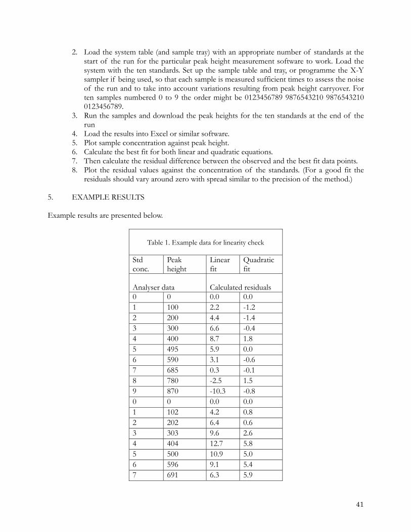
2. Load the system table (and sample tray) with an appropriate number of standards at the start of the run for the particular peak height measurement software to work. Load the system with the ten standards. Set up the sample table and tray, or programme the X-Y sampler if being used, so that each sample is measured sufficient times to assess the noise of the run and to take into account variations resulting from peak height carryover. For ten samples numbered 0 to 9 the order might be 0123456789 9876543210 9876543210 0123456789.

3. Run the samples and download the peak heights for the ten standards at the end of the run

4. Load the results into Excel or similar software. 5. Plot sample concentration against peak height. 6. Calculate the best fit for both linear and quadratic equations. 7. Then calculate the residual difference between the observed and the best fit data points. 8. Plot the residual values against the concentration of the standards. (For a good fit the

residuals should vary around zero with spread similar to the precision of the method.) 5. EXAMPLE RESULTS Example results are presented below.

Table 1. Example data for linearity check

Std conc.

Peak height

Linear fit

Quadratic fit

Analyser data

Calculated residuals

0 0 0.0 0.0 1 100 2.2 -1.2 2 200 4.4 -1.4 3 300 6.6 -0.4 4 400 8.7 1.8 5 495 5.9 0.0 6 590 3.1 -0.6 7 685 0.3 -0.1 8 780 -2.5 1.5 9 870 -10.3 -0.8 0 0 0.0 0.0 1 102 4.2 0.8 2 202 6.4 0.6 3 303 9.6 2.6 4 404 12.7 5.8 5 500 10.9 5.0 6 596 9.1 5.4 7 691 6.3 5.9

41

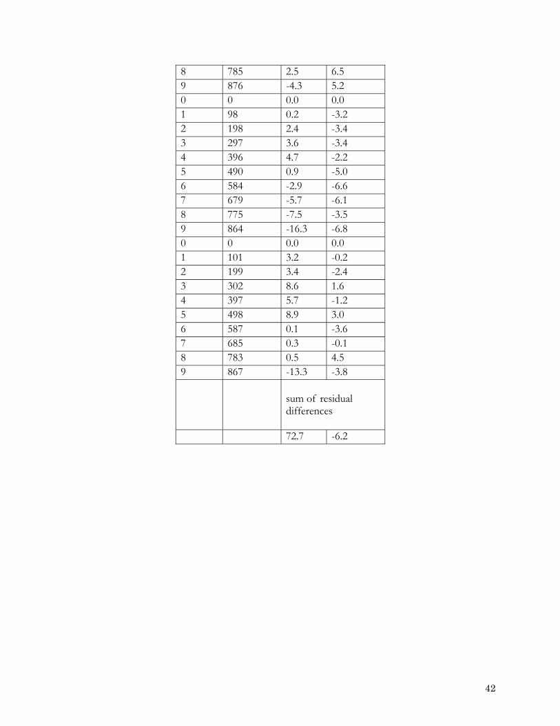
8 785 2.5 6.5 9 876 -4.3 5.2 0 0 0.0 0.0 1 98 0.2 -3.2 2 198 2.4 -3.4 3 297 3.6 -3.4 4 396 4.7 -2.2 5 490 0.9 -5.0 6 584 -2.9 -6.6 7 679 -5.7 -6.1 8 775 -7.5 -3.5 9 864 -16.3 -6.8 0 0 0.0 0.0 1 101 3.2 -0.2 2 199 3.4 -2.4 3 302 8.6 1.6 4 397 5.7 -1.2 5 498 8.9 3.0 6 587 0.1 -3.6 7 685 0.3 -0.1 8 783 0.5 4.5 9 867 -13.3 -3.8

sum of residual differences

72.7 -6.2

42

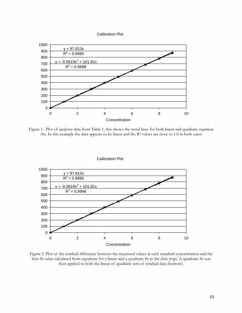
Calibration Plot

y = 97.813xR2 = 0.9995

y = -0.5619x2 + 101.81xR2 = 0.9998

0100200300400500600700800900

1000

0 2 4 6 8Concentration

10

Figure 1. Plot of analyser data from Table 1, this shows the trend lines for both linear and quadratic equation

fits. In this example the data appears to be linear and the R2 values are close to 1.0 in both cases

Calibration Plot

y = 97.813xR2 = 0.9995

y = -0.5619x2 + 101.81xR2 = 0.9998

0100200300400500600700800900

1000

0 2 4 6 8Concentration

10

Figure 2. Plot of the residual difference between the measured values at each standard concentration and the best fit value calculated from equations for a linear and a quadratic fit to the data (top). A quadratic fit was

then applied to both the linear of quadratic sets of residual data (bottom).

43

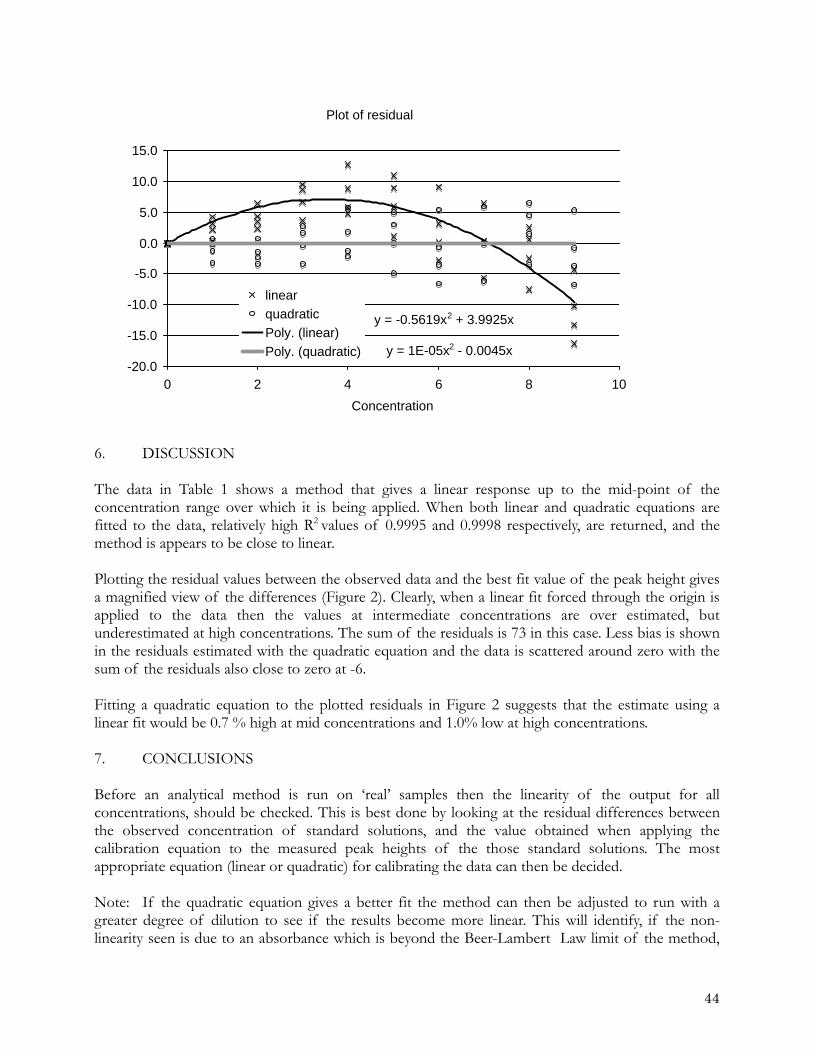
Plot of residual

y = -0.5619x2 + 3.9925x

y = 1E-05x2 - 0.0045x-20.0

-15.0

-10.0

-5.0

0.0

5.0

10.0

15.0

0 2 4 6 8Concentration

10

linearquadraticPoly. (linear)Poly. (quadratic)

6. DISCUSSION The data in Table 1 shows a method that gives a linear response up to the mid-point of the concentration range over which it is being applied. When both linear and quadratic equations are fitted to the data, relatively high R2 values of 0.9995 and 0.9998 respectively, are returned, and the method is appears to be close to linear. Plotting the residual values between the observed data and the best fit value of the peak height gives a magnified view of the differences (Figure 2). Clearly, when a linear fit forced through the origin is applied to the data then the values at intermediate concentrations are over estimated, but underestimated at high concentrations. The sum of the residuals is 73 in this case. Less bias is shown in the residuals estimated with the quadratic equation and the data is scattered around zero with the sum of the residuals also close to zero at -6. Fitting a quadratic equation to the plotted residuals in Figure 2 suggests that the estimate using a linear fit would be 0.7 % high at mid concentrations and 1.0% low at high concentrations. 7. CONCLUSIONS Before an analytical method is run on ‘real’ samples then the linearity of the output for all concentrations, should be checked. This is best done by looking at the residual differences between the observed concentration of standard solutions, and the value obtained when applying the calibration equation to the measured peak heights of the those standard solutions. The most appropriate equation (linear or quadratic) for calibrating the data can then be decided. Note: If the quadratic equation gives a better fit the method can then be adjusted to run with a greater degree of dilution to see if the results become more linear. This will identify, if the non-linearity seen is due to an absorbance which is beyond the Beer-Lambert Law limit of the method,

44

or due to an inherent problem with the linearity of output from the detector of the auto-analyser.

45

NSOP 5. DETERMINATION OF TRUE SAMPLE BLANK VALUE 1. INTRODUCTION 1.1 Definition of the blank value Following Taylor (1990) an analytical blank can be defined in the following way: A blank is the measured value for the apparent concentration of a determinand obtained when the determinand is not present in the sample at the time of measurement, that is to say the measured value for the component is due to artefacts. The blank value (which may be positive or negative) should be deducted from a measured value to give a net value due to the actual quantity of the determinand contained in the sample. The blank measurement must be made in such a way that the applied correction is valid. In order to obtain the true value for a determination it is essential to have access to the signal that would be obtained for a sample when the concentration of the determinand is zero. The sources of blank errors and problem specific to CFA analyses are considered below. It is essential that laboratories employ consistent procedures for assessing the blank values appropriate to the instrumentation that they are using and for the type of samples they are working with. 1.2 Choice of approach for CFA to determining blank values For work with samples with a small range of refractive index difference (generally open ocean samples) the approach can be simpler than when working with samples from river plumes and estuaries. Consequently two operating procedures are presented. Particularly when working at low concentrations it is critical important that the correct approach is used. 1.3 Artifacts contributing to the blank Four types of artifacts can contribute to the blank. The additive nature of these artifacts is illustrated in Figure 5.1. In order of priority for CFA analyses they are:

• Contamination of the baseline water - All baseline solutions (natural or artificial saline water or pure water) used have the potential for varying degree of contamination - even pure water can be contaminated during handling and storage.

• Refractive index blank. - A signal is generated by optically imperfect flowcells. This changes as the salinity of the samples varies (e.g. phosphate in an AAII type system an error of 0.04 μM for a 10 units change in salinity can be typical). This signal is usually positive, but negative signals can occur. In addition transient signals can be generated at the start and end of peaks when light is reflected off the interface between of waters of different density in the flow cell. This is the Schlieren effect. It can occur even in instruments in which the segmenting air bubble passes through the cell.

• Sample turbidity - A signal is generated by particles suspended in the sample. (Note: reaction with the reagents may modify the turbidity relative to that in the untreated sample.)

46

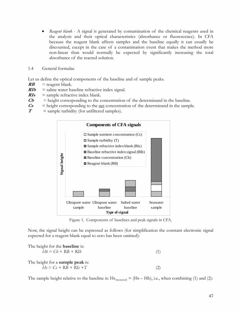
• Reagent blank - A signal is generated by contamination of the chemical reagents used in the analysis and their optical characteristics (absorbance or fluorescence). In CFA because the reagent blank affects samples and the baseline equally it can usually be discounted, except in the case of a contamination event that makes the method more non-linear than would normally be expected by significantly increasing the total absorbance of the reacted solution.

1.4 General formulae Let us define the optical components of the baseline and of sample peaks. RB = reagent blank. RIb = saline water baseline refractive index signal. RIs = sample refractive index blank. Cb = height corresponding to the concentration of the determinand in the baseline. Cs = height corresponding to the net concentration of the determinand in the sample. T = sample turbidity (for unfiltered samples).

Components of CFA signals

Ultrapure watersample

Ultrapure waterbaseline

Salted waterbaseline

Seawatersample

Type of signal

Sign

al h

eigh

t

Sample nutrient concentration (Cs)Sample turbidity (T)Sample refractive index blank (RIs)Baseline refractive index signal (RIb)Baseline concentration (Cb)Reagent blank (RB)

Figure 1. Components of baselines and peak signals in CFA.

Now, the signal height can be expressed as follows (for simplification the constant electronic signal expected for a reagent blank equal to zero has been omitted): The height for the baseline is: Hb = Cb + RB + RIb (1) The height for a sample peak is: Hs = Cs + RB + RIs +T (2) The sample height relative to the baseline is: Hs(measured) = (Hs – Hb), i.e., when combining (1) and (2):

47

Hs(measured) = Cs + RB + RIs +T – (Cb + RB + RIb) Hs(measured) = (Cs - Cb) + (RIs - RIb) +T The height corresponding to the net concentration in the sample is: Cs = Hs(measured) + Cb – (RIs - RIb + T) (3) 1.4.1 If the baseline is pure water: In that case RIb = 0, hence: Cs = Hs(measured) + Cb – [RIs + T] (4) Cb is determined by difference between the baseline signal and the signal of a freshly drawn ultra pure water (PW0). If using pure water as baseline Cb has to be determined by comparison with freshly drawn water on a regular basis. This can be done as an “extra” cup on the run. Turbidity T, which is generally negligible for oceanic waters (and = 0 for filtered samples), is measured together with the RIs (see operating procedure NSOP 5.1). The great advantage of using pure water tp provide the baseline is that pure water is easily available and Cb should be close to zero. The disadvantages are:- (1) that the refractive index blank potentially has to be determined for each saline sample, if the optics of the analyser used generate a significant refractive index blank; (2) if a Schlieren effect occurs, this can distort the peak shape and consequently increase the time each sample must be sampled for in order to achieve a stable peak height. 1.4.2 If the baseline is saline water: The idea of using a saline baseline is principally to minimise the Schlieren effect and also to avoid having to make a correction for the refractive index blank, when the samples have similar salinity.

Cs = Hs(measured) + Cb – [(RIs – RIb) + T] (3) However if the salinity of samples varies significantly and/or turbidity is not negligible, all artefacts must be determined. How large a “significant” variation in salinity is, is highly dependent on the instrumentation, the particular method being used and the precision required from it. In equation (3), (RIs – RIb) is the difference between the refractive index signal of the sample and the saline baseline. This relative refractive index blank is small and ideally (RIs – RIb) = 0 when the baseline and the samples have similar salinities. This particular case is generally achieved when working with ocean waters where the range of salinity encountered on a particular cruise will usually be small and T will also be effectively zero. In that particular case, equation (3) becomes:

Cs = Hs(measured) + Cb (5) In which case the critical aspect is the determination of Cb. 1.4.3 Determination of Cb and Rib Both Cb and RIb and must be monitored. The refractive index blank RIb should be relatively

48

invariant if the same instrument and method are being used. However Cb can potentially change each with each batch of solution used as the baseline. This can be achieved by making a set of measurements of the baseline and samples with and without colour development, so that the contribution to the signal of the background signal due to contamination and refractive index variations can be distinguished. For this a set of so called “RIs reagents” are used (see section 1.5 of this NSOP). The heights Cb and RIb are converted into concentrations by determining the sensitivity of the method S (in terms of peak measured per unit concentration of the determinand). For work with a saline water baseline four measurements of the baseline are made after the sensitivity has been determined. The procedure is described in NSOP 5.2. 1.5 The RIs (colour free) reagents The refractive index blanks (RIs and RIb) are the absorbances resulting from the differences in optical properties between fresh water and seawater in the absence of any colour development (Loder and Glibert, 1977; Froelich and Pilson, 1978). The refractive index depends on salinity, but also on reaction conditions which may affect the refractive index or the turbidity, such as the total salt content and the pH of the reagents. To measure a RIs, the signals from fresh and seawater must be compared in conditions as close as possible to those of the analysis but without any colour development. This requires that what we call ‘RIs reagents’, are prepared. They omit the one component, which is indispensable for colour development. By using RIs reagents, the optical properties of the medium are kept as similar as possible to those prevailing during the colour forming reaction. It is sometimes recommended, that pure water can be used for the RIs reagents. However this fails to accurately determine refractive index differences. Similarly, it is important to keep the wetting agent in the solutions to maintain the hydraulic stability of the flow and as the wetting agent often contributes the refractive index. Note: that if a reagent contains only the chemical that should be removed, the corresponding RIs reagent is then pure water. For example, the chemicals removed from the RIs reagents are - in the molybdenum blue methods for phosphate and silicate it is the molybdate, and in the Benschneider and Robinson’s method for nitrite (and nitrate) it is the NED (Aminot et al., 2009). 1.6 Recommendation To obtain accurate values of sample concentrations several corrections have to be applied to the raw values of sample peak heights. Minimising their number and reducing the analysis steps reduces cumulative errors and increases data quality. Working with a pure water (18 megohm.cm) baseline can help achieve this aim if the instrumentation and the method being used allow it. This requires that optical artefacts such as the Schleiren effect remain small enough to allow satisfactory measurements of the peak heights.

49

NSOP 5.1 DETERMINATION OF THE BLANK VALUE WHEN WORKING WITH SALINE SAMPLES AND USING PURE WATER TO PROVIDE THE BASELINE

MEASUREMENT. 1. SCOPE AND FIELD OF APPLICATION This NSOP describes the sequence of measurements that need to be made when pure water is used to provide the baseline measurement in a CFA system. It is appropriate for any type of water, provided the Schlieren effect does not excessively distort the peak shape. 2. PRINCIPLE Freshly drawn pure (18 megohm.cm) water is used and is assumed to contain negligible concentration of the determinand. This removes the uncertainty that is inherent in using a saline solution. In this procedure, raw sample concentrations are computed from raw heights and only the slope of the calibration curve, before the sample blanks are subtracted to provide the net concentrations. Section 1.4 of NSOP 5 shows that for baseline concentration, the size of the sample refractive index (RIs) effect and the sample turbidity (T) must be determined. Cs = height corresponding to the net concentration of the determinand in the sample. Cs = Hs(measured) + Cb – [RIs + T] (4) Where Hs = height of sample peak Hb = height of pure water baseline with complete reagents HbPW0 = height of freshly drawn pure water sample with complete reagents, Cb = height corresponding to the concentration of the determinand in the baseline. Cb = Hb - HbPW0 Hb(RIs) = height of pure water baseline with RIs reagents Hs(RIs) = height of sample peak with RIs reagents, For each sample (RIs + T) =(Hs(RIs) - Hb(RIs)) Figure 1 of this NSOP illustrates the determination of these artifacts. 3. EQUIPMENT Standard Continuous Flow Analyzer (CFA) equipment 4. REAGENTS

• Stock standards of the specific nutrient • Baseline solution - pure water

50

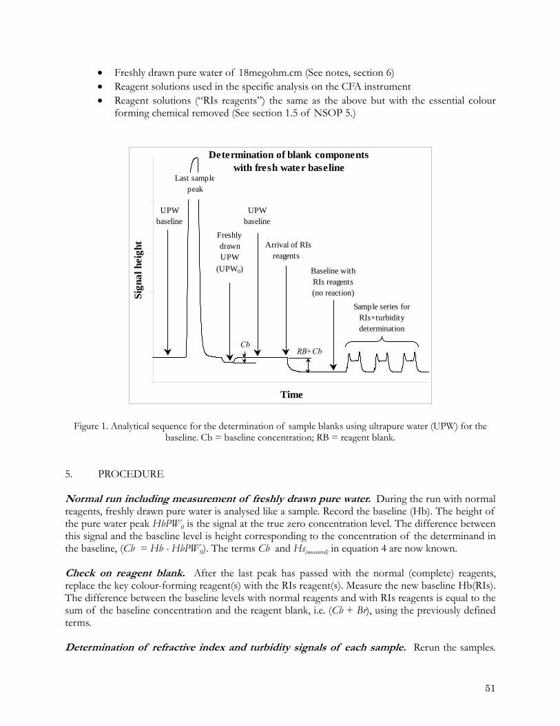
• Freshly drawn pure water of 18megohm.cm (See notes, section 6) • Reagent solutions used in the specific analysis on the CFA instrument • Reagent solutions (“RIs reagents”) the same as the above but with the essential colour

forming chemical removed (See section 1.5 of NSOP 5.)

Time

Sign

al h

eigh

t

FreshlydrawnUPW

(UPW0) Baseline withRIs reagents(no reaction)

Arrival of RIsreagents

Sample series forRIs+turbiditydetermination

RB+Cb

Last samplepeak

UPWbaseline

UPWbaseline

Cb

Determination of blank components with fresh water baseline

Figure 1. Analytical sequence for the determination of sample blanks using ultrapure water (UPW) for the baseline. Cb = baseline concentration; RB = reagent blank.

5. PROCEDURE Normal run including measurement of freshly drawn pure water. During the run with normal reagents, freshly drawn pure water is analysed like a sample. Record the baseline (Hb). The height of the pure water peak HbPW0 is the signal at the true zero concentration level. The difference between this signal and the baseline level is height corresponding to the concentration of the determinand in the baseline, (Cb = Hb - HbPW0). The terms Cb and Hs(measured) in equation 4 are now known. Check on reagent blank. After the last peak has passed with the normal (complete) reagents, replace the key colour-forming reagent(s) with the RIs reagent(s). Measure the new baseline Hb(RIs). The difference between the baseline levels with normal reagents and with RIs reagents is equal to the sum of the baseline concentration and the reagent blank, i.e. (Cb + Br), using the previously defined terms. Determination of refractive index and turbidity signals of each sample. Rerun the samples.

51

Record the peak heights Hs(RIs). For each sample Hs(RIs) corresponds to the sum of refractive index and the turbidity, Hs(RIs) = (RIs + T) see equation 4. Calculation. By combining the results of stages 1 and 3, equation 4 is now solved and Cs is now known for each sample and can then used in the normal way to calculate the results. 6. NOTES Dissolved silicate can be present in ultra pure water even if the conductivity reading on the dispensing unit is 18 megohm.cm. Therefore the blank determination for silicate should be done with water obtained from equipment where the purification cartridges are known to have been recently replaced. The omitted chemicals (“essential chemicals”) are: PO4 Ammonium Molybdate Si Ammonium Molybdate NOx NED NO2 NED NH4 Sodium Hypochlorite Usually, Cb = 0, but contamination may occur for ammonium (from handling) and silicate (from aged ion exchange resins). In general, with oceanic waters of sample salinity and turbidity are similar so that differences of [RIB+T] among samples are insignificant and only a few representative samples need to be checked to obtain that value.

52

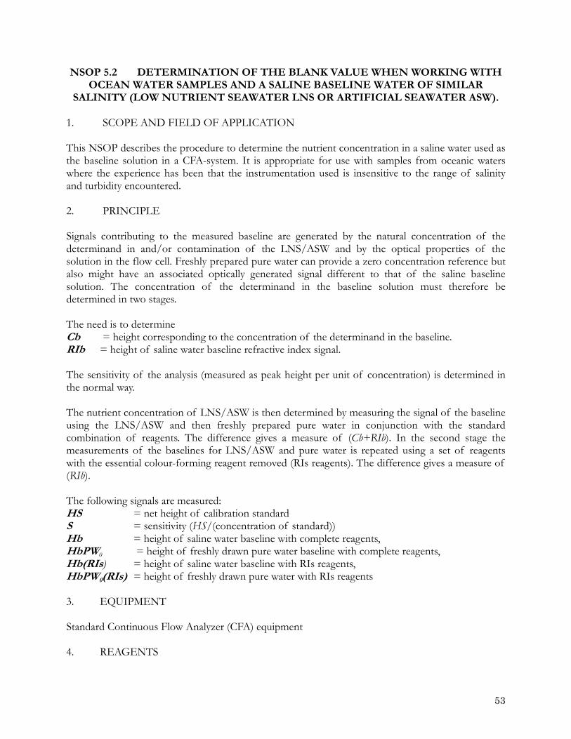
NSOP 5.2 DETERMINATION OF THE BLANK VALUE WHEN WORKING WITH OCEAN WATER SAMPLES AND A SALINE BASELINE WATER OF SIMILAR

SALINITY (LOW NUTRIENT SEAWATER LNS OR ARTIFICIAL SEAWATER ASW). 1. SCOPE AND FIELD OF APPLICATION This NSOP describes the procedure to determine the nutrient concentration in a saline water used as the baseline solution in a CFA-system. It is appropriate for use with samples from oceanic waters where the experience has been that the instrumentation used is insensitive to the range of salinity and turbidity encountered. 2. PRINCIPLE Signals contributing to the measured baseline are generated by the natural concentration of the determinand in and/or contamination of the LNS/ASW and by the optical properties of the solution in the flow cell. Freshly prepared pure water can provide a zero concentration reference but also might have an associated optically generated signal different to that of the saline baseline solution. The concentration of the determinand in the baseline solution must therefore be determined in two stages. The need is to determine Cb = height corresponding to the concentration of the determinand in the baseline. RIb = height of saline water baseline refractive index signal. The sensitivity of the analysis (measured as peak height per unit of concentration) is determined in the normal way. The nutrient concentration of LNS/ASW is then determined by measuring the signal of the baseline using the LNS/ASW and then freshly prepared pure water in conjunction with the standard combination of reagents. The difference gives a measure of (Cb+RIb). In the second stage the measurements of the baselines for LNS/ASW and pure water is repeated using a set of reagents with the essential colour-forming reagent removed (RIs reagents). The difference gives a measure of (RIb). The following signals are measured: HS = net height of calibration standard S = sensitivity (HS/(concentration of standard)) Hb = height of saline water baseline with complete reagents, HbPW0 = height of freshly drawn pure water baseline with complete reagents, Hb(RIs) = height of saline water baseline with RIs reagents, HbPW0(RIs) = height of freshly drawn pure water with RIs reagents 3. EQUIPMENT Standard Continuous Flow Analyzer (CFA) equipment 4. REAGENTS

53

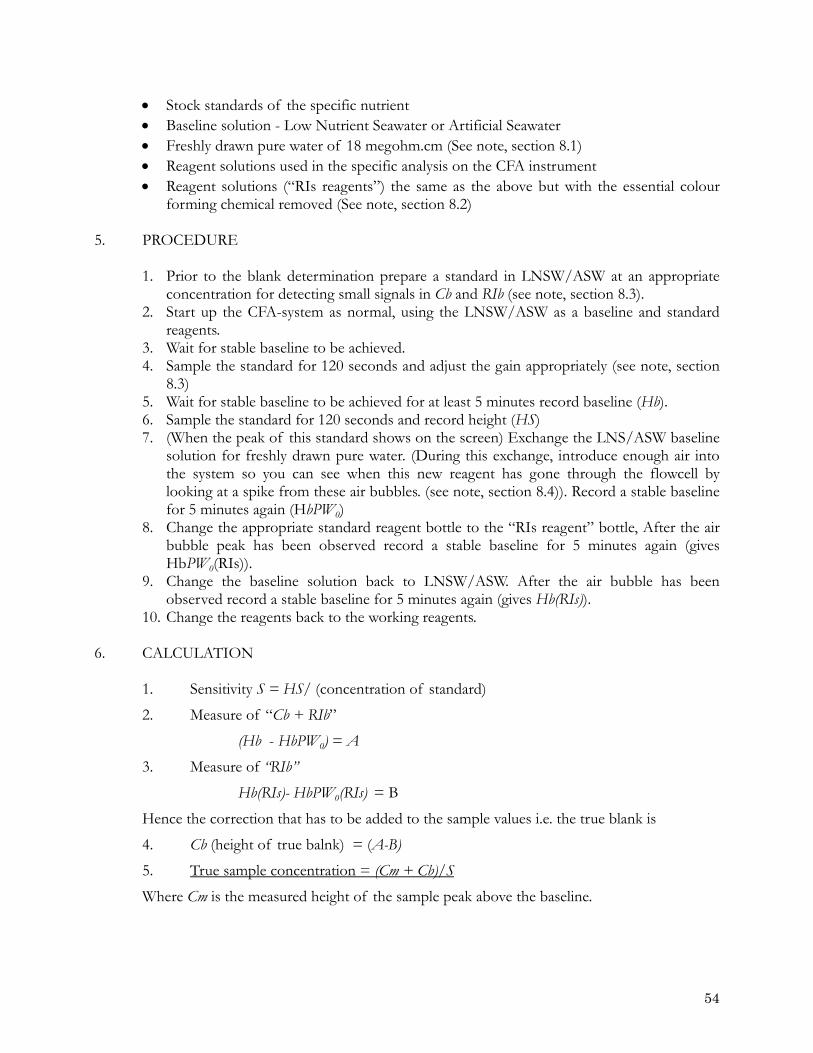
• Stock standards of the specific nutrient • Baseline solution - Low Nutrient Seawater or Artificial Seawater • Freshly drawn pure water of 18 megohm.cm (See note, section 8.1) • Reagent solutions used in the specific analysis on the CFA instrument • Reagent solutions (“RIs reagents”) the same as the above but with the essential colour

forming chemical removed (See note, section 8.2) 5. PROCEDURE

1. Prior to the blank determination prepare a standard in LNSW/ASW at an appropriate concentration for detecting small signals in Cb and RIb (see note, section 8.3).

2. Start up the CFA-system as normal, using the LNSW/ASW as a baseline and standard reagents.

3. Wait for stable baseline to be achieved. 4. Sample the standard for 120 seconds and adjust the gain appropriately (see note, section

8.3) 5. Wait for stable baseline to be achieved for at least 5 minutes record baseline (Hb). 6. Sample the standard for 120 seconds and record height (HS) 7. (When the peak of this standard shows on the screen) Exchange the LNS/ASW baseline

solution for freshly drawn pure water. (During this exchange, introduce enough air into the system so you can see when this new reagent has gone through the flowcell by looking at a spike from these air bubbles. (see note, section 8.4)). Record a stable baseline for 5 minutes again (HbPW0)

8. Change the appropriate standard reagent bottle to the “RIs reagent” bottle, After the air bubble peak has been observed record a stable baseline for 5 minutes again (gives HbPW0(RIs)).

9. Change the baseline solution back to LNSW/ASW. After the air bubble has been observed record a stable baseline for 5 minutes again (gives Hb(RIs)).

10. Change the reagents back to the working reagents. 6. CALCULATION

1. Sensitivity S = HS/ (concentration of standard)

2. Measure of “Cb + RIb” (Hb - HbPW0) = A

3. Measure of “RIb”

Hb(RIs)- HbPW0(RIs) = B

Hence the correction that has to be added to the sample values i.e. the true blank is

4. Cb (height of true balnk) = (A-B) 5. True sample concentration = (Cm + Cb)/S

Where Cm is the measured height of the sample peak above the baseline.

54

7. CAUTION As the baseline water can be contaminated during handling and storage this means that depending on the working conditions, the background level of nutrients may not be the same in the LNS/ASW used to prepare the working standards as that in the baseline LNS/ASW, being pumped through the analyser - even though both came from the same bulk solution at some point in time. Effort should be made to minimise such discrepancies. A way to do this is to determine the calibration (zero) blank as one of the set of measured calibration standards. It should be determined on LNS/ASW drawn from the bulk solution providing the baseline at the same time as the water used to prepare the spiked standards and should be handled and stored in the same way. 8. NOTES

1. Dissolved silicate can be present in ultra pure water even if the conductivity reading on the dispensing unit is 18 megohm.cm. Therefore the blank determination for silicate should be done with water obtained from equipment where the purification cartridges are known to have been recently replaced.

2. The omitted chemicals (“essential chemicals”) are:

PO4 Ammonium Molybdate Si Ammonium Molybdate NOx NED NO2 NED NH4 Sodium Hypochlorite

3. The calibration standard should be at an appropriate concentration for detecting small signals in Cb and RIb. For measurement of at macro nutrient concentrations in ocean water for silicate and nitrate a standard concentration of 5 µM l-1 would be appropriate and for phosphate 1 µM l-1 with the peak height adjusted to give full scale “deflection”. Those determining micro-nutrient concentration would work with lower concentration standards.

4. Marking the change over by introducing extra air should be done with each change-over of

baseline solution and reagents. 9. REFERENCES Aminot, A., Kérouel, R and Coverly, S.C. 2009. Nutrients in seawater using segmented flow analysis.

Chapter 9 in Practical Guidelines for the Analysis of Seawater. Wurl, O., ed. USA: CRC Press. In press.

Froelich, P.N. and Pilson, M.E.Q. 1978. Systematic absorbance errors with Technicon Autoanalyzer

II colorimeters. Water Research 12, 599-603. Loder, T.C. and. Glibert, P.M. 1977. Blank and salinity corrections for automated nutrient analysis of

55

56

estuarine and seawaters. Pp. 48-56 in Advances in automated analysis. 7th Technicon International Congress, December, 13-15, 1976.

Taylor, J.K, 1990. Quality assurance of chemical measurements. USA: Lewis Publishers, Inc., 328 p.

NSOP 7 - Water sampling and storage of samples for the determination of concentrations of nutrients in seawater

NSOP 6. IMPROVING THE INTER-RUN PRECISION OF NUTRIENT MEASUREMENT BY USE OF A TRACKING STANDARD

1. SCOPE AND FIELD OF APPLICATION This NSOP describes the procedure developed at RNIOZ (Texel, Netherlands), which uses results from measurements of a stable artificial standard solution made through out a cruise to adjust the data and there by improve inter-run precision. 2. PRINCIPLE The assumption are (1) that the preparation of so called “tracking” standard solution by single dilution of stable mixed standard solution can produce a solution containing concentrations of nutrients which are less variable than the calibration relationship measured on each run of a CFA system measuring nutrient during a cruise; (2) if this precisely prepared solution is measured on each run then the output from each run can be adjusted by the ratio between the concentration of the standard measured on that run and the average of all runs, in order to improve the overall precision of the measurements during the cruise. 3. EQUIPMENT

• Volumetric flask calibrated to 0.01 % • Dispensing pipette calibrated and with a precision of 0.1 % • Thermometer reading to 0.1oC

4. REAGENTS

• Mixed secondary standard containing know amounts of nitrate, phosphate and silicate preserved by the addition of Mercuric Chloride to a concentration of 0.02 g l-1 (HgCl2)

• Low nutrient seawater or sodium chloride solution (40 g l-1) 5. PROCEDURE

1. Prior to each run of the CFA system prepare a fresh tracking standard recording the temperature. The concentration should be chosen to be about 80 % of that of the top standards.

2. During the run measure the standard a minimum of three times spaced through the run. 3. At the end of the run record the mean value for the standard. 4. Validate the use of the standard by measuring in duplicate the deepest sample taken from

the rosette on the analytical run for the samples from that rosette cast. 5. For the validation repeat the measurement of the duplicated deep sample on the run for

samples from the next cast. 6. During the cruise prepare a control chart for the values of the tracking standard. 7. At the end of the cruise calculate the mean value for the tracking standard. 8. For each analytical run calculate the ratio of the value of the tracking standard on that

run to the mean value of the tracking standard for the cruise. 9. Adjust the values for each run by the ratio of the tracking standard values.

57

NSOP 7 - Water sampling and storage of samples for the determination of concentrations of nutrients in seawater

10. Compare the route mean square value of the difference between measurements of the deep sample duplicates measured in a run and the difference between run.

11. Use of the tracking standard is acceptable if the root mean square differences are smaller after adjustment to the tracker standard value.

6. NOTES All details of this adjustment process and the control chart of the tracer values should be include as part of the cruise meta-data set. Alternatively RMNS materials produced from the same batch can be used to the same effect as the tracking standards, however due to cost implications it is normally the case to use a tracking standard on this regular basis but then compare and check against a RMNS standard every few days during a cruise, hence this links the tracking standards and the RMNS solutions, and hence calibrates the tracking standard also. Details of these results should also be logged and compared as before.

58

NSOP 7 - Water sampling and storage of samples for the determination of concentrations of nutrients in seawater

NSOP 7. WATER SAMPLING AND STORAGE OF SAMPLES FOR THE DETERMINATION OF CONCENTRATIONS OF NUTRIENTS IN SEAWATER

1. SCOPE AND FIELD OF APPLICATION This NSOP describes how to collect discrete samples, from a Niskin or other water sampler, that are suitable for the analysis of dissolved nutrients - nitrate, nitrite, phosphate and silicate. It also describes how samples should be stored after collection if necessary. 2. PRINCIPLE A sample of seawater is collected in a sterile plastic container that can be tightly sealed for short or long term storage. 3. APPARATUS Water Samplers At the beginning of a cruise leg and at weekly intervals, the water samplers should be inspected for evidence of biological and damaged components. Any rust should be removed and damaged components replaced. Microbial films should be removed using a soft sponge and Decon 90. (Brushes, and scouring agents and pads must not be used as they will damage the surface of the bottle and increase the likelihood of future contamination). Drawing tube Tygon tubing is normally used to transfer the sample from the Niskin to the sample container; however, if dissolved organic carbon samples are being collected from the same Niskins, then it may be necessary to use silicone tubing to prevent contamination from the Tygon. When oxygen samples are also being collected the drawing tube should be pre-treated by soaking in clean seawater for at least one day. This minimizes the amount of bubble formation in the tube when drawing a sample. Sample container The largest errors occur in nutrient analysis tend to be due to poor choice of sample containers, compounded by inappropriate storage. Seawater as it comes from the sampling apparatus on the ship is a relatively sterile solution, particularly when sampled below the thermocline and will therefore be slow to change if placed in a sterile container. It is therefore a gross error to put samples into non-sterile containers. That is any container other than an autoclaved one that has been used previously. Disposable containers such 30ml Coulter Counter vials provide a simple source of sterile containers when used once and then disposed of. It is essential that you check your chosen containers both for contamination and sterility. 4. PROCEDURE 4.1 Introduction The order in which different samples are taken from the Niskin bottle will decided by the principal scientist on the cruise taking into consideration the stability of the components being sampled for. Nutrients are relatively stable and will normally be sampled towards the end of the process before salinity samples are drawn.

59

NSOP 7 - Water sampling and storage of samples for the determination of concentrations of nutrients in seawater

4.2 Filling procedure • Fill a sample vial rack - with an appropriate number of vials for the number of bottles on

the rosette and the number of duplicates to be taken. • Clearly label each sample vial with the bottle number and a unique identity for the cast. • Check that the drawing tube is clean - replace if necessary • Rinse the sample container — Rinse the container and its lid twice with half to a third

the volume of the container of sample • Fill the sample container three quarters full. • Check the headspace — Check the vial has not been over filled, a head space is necessary

if subsequently samples need to be frozen. Firmly tighten the container’s lid 4.3 Sample documentation The following information must be recorded in the sampling logbook at the time of sampling:

• Time and date when taken. • Full name of person who took sample. • Location: an unambiguous designation of the station, cast, and the rosette position from

which the sample was taken. • Container designation: a number or alphanumeric symbol unique to the sample

container; and the cruise. • Comments: additional information such as conditions when sampling, problems with

sample collection, etc. 5. SAMPLE STORAGE During a cruise samples should be stored in a cool, dark, location (preferably refrigerated but not frozen) until use. Ideally nutrient samples should be analysed immediately after sampling to avoid any possibility of biological growth or decay in the samples. 5.1 Sample storage with freezing If storage is necessary for more than a two to three days samples should be frozen as soon after collection and as rapidly as possible. Before freezing ensure that sample bottles are no more than 3/4 full and firmly capped. A deep freezer (at least -20 oC) should be used. Good air circulation around the bottles in the freezer is important. Sample pots should be retained in labeled gridded racks, so that they can be easily found and sorted for analysis when they the time has come to measure them Samples should be thawed in air. Water baths should not be used because of the danger of contamination from tap water. As the sample melts and comes to room temperature it volume goes through a minimum the resulting low pressure in the containers can suck in contaminating water from a water bath. Samples for the determination of Si should be allowed to stand for at least 24 hours at room temperature for de-polymerisation to occur. For work at higher (>40 mM/m3) concentrations you should check that your freezing and thawing procedures are appropriate.

60

NSOP 7 - Water sampling and storage of samples for the determination of concentrations of nutrients in seawater

61

6. QUALITY ASSURANCE Duplicate sampling is recommended, both from the same sampler (e.g., Niskin bottle) and if possible, from two (Niskin) samplers tripped together at the same depth, to assess the quality of the sampling procedures. It is important that the time at which a sample was measured is recorded in the meta-data. This will potentially allow discrepant data resulting from in appropriately long storage to be identified..

NSOP 8. WATER SAMPLING AND STORAGE OF SAMPLES FOR THE DETERMINATION OF LOW CONCENTRATIONS OF NUTRIENTS IN SEAWATER

1. SCOPE AND FIELD OF APPLICATION This SOP describes how to collect discrete samples, from a Niskin bottle or other water samplers that are suitable for the analysis of low concentrations dissolved nutrients - ammonium, nitrate, nitrite and phosphate. It also describes how samples should be stored after collection if this cannot be avoided. The recommendation is that samples are not stored. 2. PRINCIPLE A sample of seawater is collected in a clean, ‘aged’, sterile plastic (HDPE) container that can be tightly sealed for short or long term storage. 3. APPARATUS Water Samplers At the beginning of a cruise leg and at weekly intervals, the water samplers should be inspected for evidence of biological and damaged components. Only water samples with external springs should be used. Any rust should be removed and damaged components replaced. Microbial films should be removed using a soft sponge and Decon 90. (Brushes, and scouring agents and pads must not be used as they will damage the surface of the bottle and increase the likelihood of future contamination). Drawing tube For low concentration samples and dissolved organic carbon samples to transfer the sample from the Niskin to the sample container; “aged” silicon tubing should be used (Tygon tubing can generate contamination). When oxygen samples are also being collected the drawing tube should be pre-treated by soaking in clean seawater for at least one day. This minimizes the amount of bubble formation in the tube when drawing a sample. Sample container The largest errors occur in nutrient analysis tend to be due to poor choice of sample containers, compounded by inappropriate storage. Seawater as it comes from the sampling apparatus on the ship is a relatively sterile solution, particularly when sampled below the thermocline. It is therefore a gross error to put samples into non-sterile containers. You must check and document how well the containers you use do their job with respect to both contamination and loss of nutrients. 4. PROCEDURE 4.1 Introduction The order in which different samples are taken from the Niskin bottle will decided by the Principal Scientist on the cruise taking into consideration the stability of the components being sampled for. Nutrients are relatively stable and will normally be sampled towards the end of the process before salinity samples are drawn. However, for ammonium analysis and for nanomolar nitrate, nitrite and phosphate then the sampling should be as soon as possible to allow on-board analysis to take place

62

immediately. In this case the nutrients would be sampled after any gas sampling procedures. It is imperative that the gloves worn for nutrient sampling are clean and non-contaminating. They should be tested by leaving in Milli-Q water and then analysing to see if the gloves proposed actually leach any nutrients out. Any persons sampling before the nutrients should also wear the appropriate gloves. 4.2 Filling procedure

• Fill a sample vial rack - with an appropriate number of vials for the number of bottles on the rosette and the number of duplicates to be taken.

• Clearly label each samples vial with a unique identity for the cruise, and the sampling event.

• Check that the drawing tube is clean – clean thoroughly or replace if necessary • Rinse the sample bottle — Rinse the vial and its lid thrice (with a third to half the

container volume sample. • Fill the sample bottle — Fill the vial three quarters full. • Check the headspace — Check the vial has not been over filled, a head space is necessary

if subsequently samples need to be frozen. Firmly tighten the vial’s lid. 4.3. Sample documentation The following information must be recorded in the sampling logbook at the time of sampling:

• Time and date when taken. • Full name of person who took sample. • Location: an unambiguous designation of the station, cast, and bottle number from

which the sample was taken. • Container designation: a number or alphanumeric symbol unique to the sample

container; and the cruise. • Comments: additional information such as conditions when sampling, problems with

sample collection, etc.

5. SAMPLE STORAGE Ideally nutrient samples should be analysed immediately after sampling to avoid any possibility of biological growth or decay in the samples. If necessary, samples should be stored in a cool, dark, location (preferably refrigerated but not frozen) until use, but ideally no longer than 1-2 hours. 5.1 Sample storage with freezing If storage is necessary samples should be frozen as soon after collection and as rapidly as possible. Before freezing ensure that sample bottles are no more than 3/4 full and firmly capped. A deep freezer (at least -20 oC) should be used. Good air circulation around the bottles in the freezer is important. Sample pots should be retained in labelled gridded racks, so that they can be easily found and sorted for analysis when they the time has come to measure them. Samples should be thawed in air. Water baths should not be used because of the danger of contamination from tap water. As the sample melts and comes to room temperature it volume goes

63

through a minimum the resulting low pressure in the containers can suck in contaminating water from a water bath. Samples for the determination ammonium, nitrate and phosphate are best measured as soon as the possible after thawing. It is recommended that a series of internal standards are added to the samples before freezing to act as a freezing ‘tracking standard’, this can show how well the samples have survived the freezing process and what artifacts have occurred as a result. 6. QUALITY ASSURANCE Duplicate sampling is recommended, both from the same sampler (e.g., Niskin bottle) and, if possible, from two Niskin bottle samplers tripped together at the same depth, to assess the quality of the sampling procedures. It is important that the time at which a sample was measured is recorded in the meta-data. This will potentially allow discrepant data resulting from inappropriately long storage to be identified..

64

NSOP 9. EXAMPLE SOP FOR SHIPBOARD OPERATION OF A CFA SYSTEM 1. SCOPE AND FIELD OF APPLICATION This SOP describes the standardised set up of one laboratory’s system for the shipboard determination of nutrients (nitrate + nitrite, nitrite, phosphate and silicate). An SOP of this type should be part of the meta-data reported at the end of each cruise. Each laboratory’s SOP should be updated as necessary before a cruise and the procedures outlined in the SOP followed during the cruise. 2. PRINCIPLE The purpose of this SOP is to provide a record of how a CFA system was operated during a cruise. It should ensure that work on the cruise is carried out in a consistent and reproducible manner. It should also ensure that key procedures that aid in maintaining the relative accuracy of data such as the calibration of volumetric ware and pipettes are carried and documented in traceable way prior to and post cruise. 3. EXAMPLE STANDARD OPERATING PROCEDURES FOR SEA GOING AUTO-

ANALYSER USE PREPARED BY MARINE WORKS, JAPAN LTD., FOR THE USE OF A “BRAN AND LUEBBE TRAACS 800” SYSTEM AT SEA

3.1 Methods The analytical methods of the nutrients during this cruise are similar with previous cruises (Aoyama et al., 2005). Nitrate + nitrite: Nitrate + nitrite and nitrite are analyzed following a modification of the method of Grasshoff (1970). The sample nitrate is reduced to nitrite in a cadmium tube the inside of which is coated with metallic copper. The sample stream after reduction is treated with an acidic, sulfanilamide reagent to produce a diazonium ion. N-1-Naphthylethylene-diamine added to the sample stream to produce a red azo dye. With reduction of the nitrate to nitrite, both nitrate and nitrite react and are measured; without reduction, only nitrite reacts. Thus, for the nitrite analysis, no reduction is performed and the alkaline buffer is not necessary. Nitrate is computed by difference. Silicate: The silicate method is analogous to that described for phosphate. The method used is essentially that of Grasshoff et al. (1983). Silicomolybdic acid is first formed from the silicate in the sample and molybdic acid. The silicomolybdic acid is reduced to silicomolybdous acid, or "molybdenum blue," using ascorbic acid. Phosphate: The phosphate analysis is a modification of the procedure of Murphy and Riley (1962). Molybdic acid is added to the seawater sample to form phosphomolybdic acid which is in turn reduced to phosphomolybdous acid using L-ascorbic acid as the reductant. The flow diagrams and reagents for each parameter are shown in Figures 1-4 below.

65

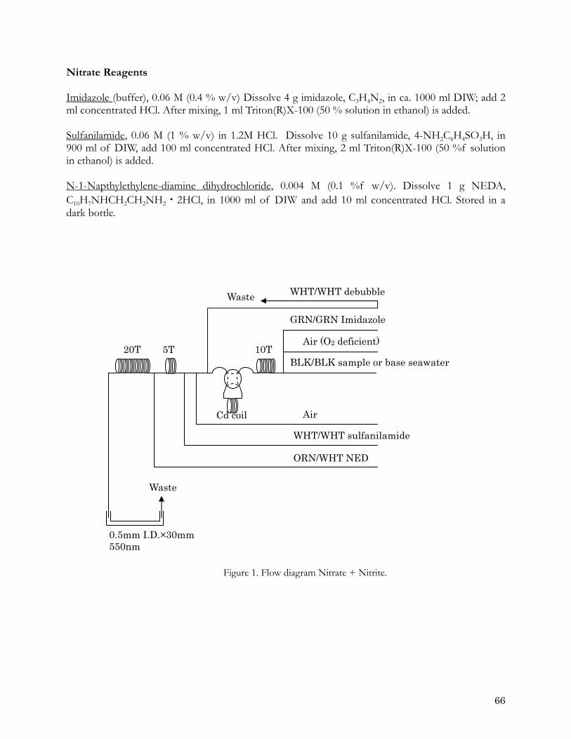
Nitrate Reagents Imidazole (buffer), 0.06 M (0.4 % w/v) Dissolve 4 g imidazole, C3H4N2, in ca. 1000 ml DIW; add 2 ml concentrated HCl. After mixing, 1 ml Triton(R)X-100 (50 % solution in ethanol) is added. Sulfanilamide, 0.06 M (1 % w/v) in 1.2M HCl. Dissolve 10 g sulfanilamide, 4-NH2C6H4SO3H, in 900 ml of DIW, add 100 ml concentrated HCl. After mixing, 2 ml Triton(R)X-100 (50 %f solution in ethanol) is added. N-1-Napthylethylene-diamine dihydrochloride, 0.004 M (0.1 %f w/v). Dissolve 1 g NEDA, C10H7NHCH2CH2NH2・2HCl, in 1000 ml of DIW and add 10 ml concentrated HCl. Stored in a dark bottle.

ORN/WHT NED

Figure 1. Flow diagram Nitrate + Nitrite.

BLK/BLK sample or base seawater

Cd coil

10T5T 20T

WHT/WHT debubbleWaste

GRN/GRN Imidazole

Air (O2 deficient)

Air

WHT/WHT sulfanilamide

Waste

0.5mm I.D.×30mm 550nm

66

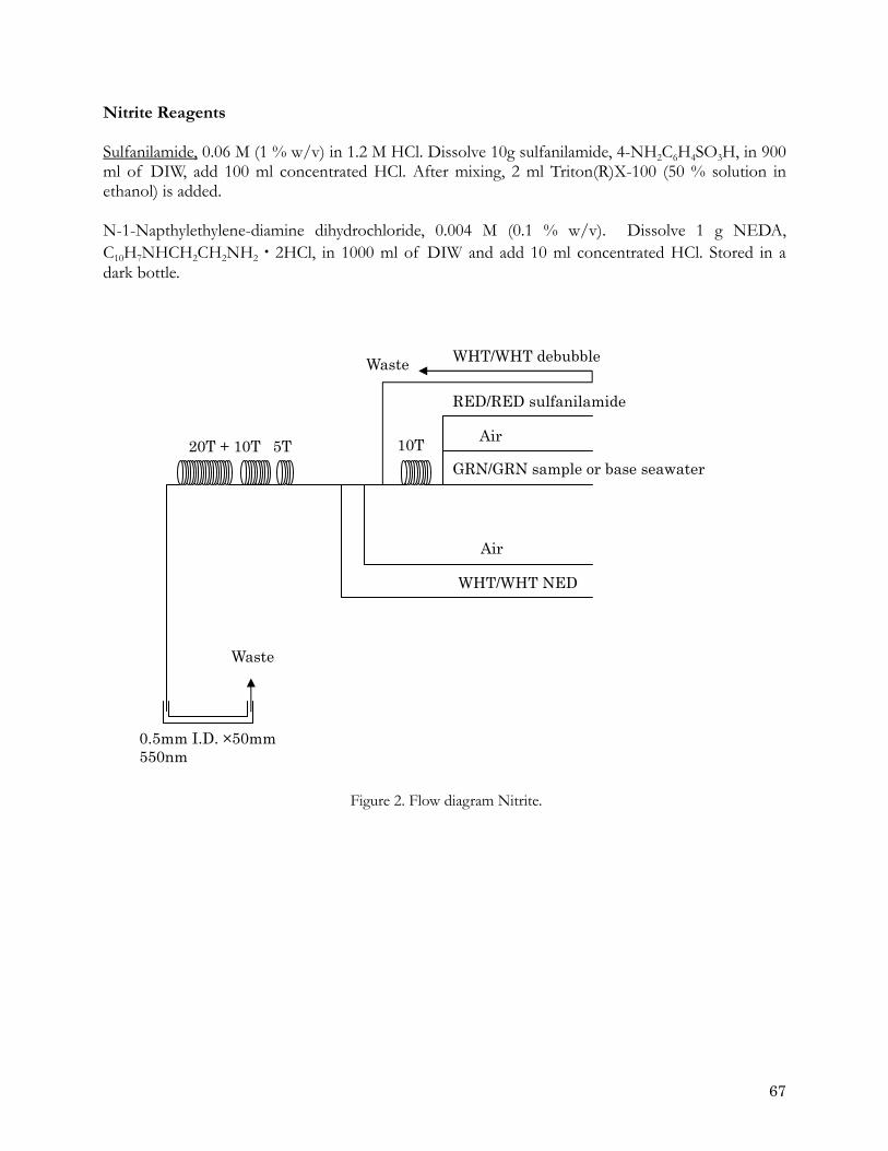
Nitrite Reagents Sulfanilamide, 0.06 M (1 % w/v) in 1.2 M HCl. Dissolve 10g sulfanilamide, 4-NH2C6H4SO3H, in 900 ml of DIW, add 100 ml concentrated HCl. After mixing, 2 ml Triton(R)X-100 (50 % solution in ethanol) is added. N-1-Napthylethylene-diamine dihydrochloride, 0.004 M (0.1 % w/v). Dissolve 1 g NEDA, C10H7NHCH2CH2NH2・2HCl, in 1000 ml of DIW and add 10 ml concentrated HCl. Stored in a dark bottle.

WHT/WHT debubbleWaste

RED/RED sulfanilamide

Air 10T 20T + 10T 5T GRN/GRN sample or base seawater

Air

WHT/WHT NED

Waste

0.5mm I.D. ×50mm 550nm

Figure 2. Flow diagram Nitrite.

67

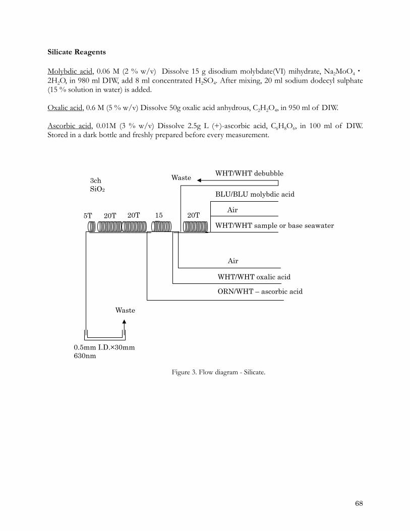
Silicate Reagents Molybdic acid, 0.06 M (2 % w/v) Dissolve 15 g disodium molybdate(VI) mihydrate, Na2MoO4・2H2O, in 980 ml DIW, add 8 ml concentrated H2SO4. After mixing, 20 ml sodium dodecyl sulphate (15 % solution in water) is added. Oxalic acid, 0.6 M (5 % w/v) Dissolve 50g oxalic acid anhydrous, C2H2O4, in 950 ml of DIW. Ascorbic acid, 0.01M (3 % w/v) Dissolve 2.5g L (+)-ascorbic acid, C6H8O6, in 100 ml of DIW. Stored in a dark bottle and freshly prepared before every measurement.

WHT/WHT debubbleWaste

BLU/BLU molybdic acid

0.5mm I.D.×30mm

Air20T20T

WHT/WHT sample or base seawater 20T 5T 15

T

3ch SiO2

Air

WHT/WHT oxalic acid

ORN/WHT – ascorbic acid

Waste

630nm

Figure 3. Flow diagram - Silicate.

68

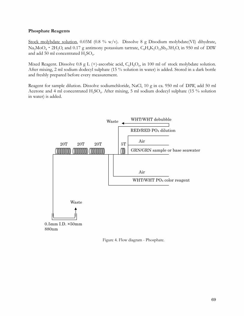
Phosphate Reagents Stock molybdate solution, 0.03M (0.8 % w/v). Dissolve 8 g Disodium molybdate(VI) dihydrate, Na2MoO4・2H2O, and 0.17 g antimony potassium tartrate, C8H4K2O12Sb2.3H2O, in 950 ml of DIW and add 50 ml concentrated H2SO4. Mixed Reagent. Dissolve 0.8 g L (+)-ascorbic acid, C6H8O6, in 100 ml of stock molybdate solution. After mixing, 2 ml sodium dodecyl sulphate (15 % solution in water) is added. Stored in a dark bottle and freshly prepared before every measurement. Reagent for sample dilution. Dissolve sodiumchloride, NaCl, 10 g in ca. 950 ml of DIW, add 50 ml Acetone and 4 ml concentrated H2SO4. After mixing, 5 ml sodium dodecyl sulphate (15 % solution in water) is added.

Figure 4. Flow diagram - Phosphate.

5T 20T 20T

WHT/WHT debubble

RED/RED PO4 dilution

Air

GRN/GRN sample or base seawater

Air

WHT/WHT PO4 color reagent

Waste

Waste

0.5mm I.D. ×50mm 880nm

20T

69

3.2 Sampling procedures Sampling of nutrients followed that oxygen, trace gases and salinity. Samples were drawn into two of virgin 10 ml polyacrylates vials without sample drawing tubes. These were rinsed three times before filling and vials were capped immediately after the drawing. The vials are put into water bath at 24 ± 1deg. C in 10 minutes before use to stabilize the temperature of samples in both MR0704 and MR0706. No transfer was made and the vials were placed directly into an auto sampler tray. Samples were analyzed after collection basically within 20 hours in MR0704 and 14 hours in MR0706. 3.3 Data processing Raw data from TRAACS800 were treated as follows:

1. Check baseline shift. 2. Check the shape of each peak and positions of peak values taken, and then change the

positions of peak values taken if necessary. 3. Calibration curves to get nutrients concentration were assumed second order equations. 4. Carry-over correction and baseline drift correction were applied to peak heights of each

samples followed by sensitivity correction. 5. Baseline correction and sensitivity correction were done basically using liner regression. 6. Load pressure and salinity from CTD data to calculate density of seawater and convert

data from μM/l to μM /kg 3.4 Nutrients standards 3.4.1 Volumetric Laboratory Ware and preparation of in-house standards All volumetric glass- and polymethylpentene (PMP)-ware used were gravimetrically calibrated. Plastic volumetric flasks were gravimetrically calibrated at a temperature within 2-3oC of the ship’s laboratory temperature (21 oC. Volumetric flasks of Class quality (Class A) are used because their nominal tolerances are 0.05 % or less over the size ranges likely to be used in this work. Class A flasks are made of borosilicate glass. The computation of volume contained by glass flasks at various temperatures other than the calibration temperatures were done by using the coefficient of linear expansion of borosilicate crown glass. The weights obtained in the calibration weightings were corrected for the density of water and air buoyancy. To prevent excessive dissolution of silicate from the glass, the standard solutions were transferred to plastic bottles as quickly as possible after they are made up to volume and well mixed. 3.4.2 Pipettes All pipettes have nominal calibration tolerances of 0.1 % or better. These were gravimetrically calibrated in order to verify and improve upon this nominal tolerance, before and after the cruise.

70

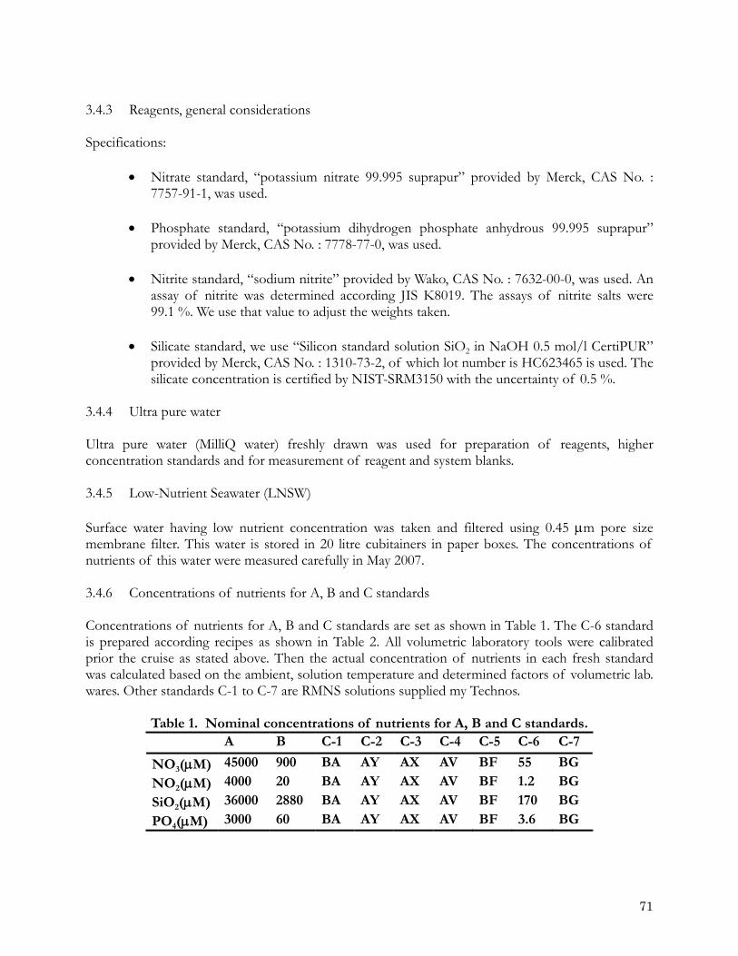
3.4.3 Reagents, general considerations Specifications:

• Nitrate standard, “potassium nitrate 99.995 suprapur” provided by Merck, CAS No. : 7757-91-1, was used.

• Phosphate standard, “potassium dihydrogen phosphate anhydrous 99.995 suprapur”

provided by Merck, CAS No. : 7778-77-0, was used.

• Nitrite standard, “sodium nitrite” provided by Wako, CAS No. : 7632-00-0, was used. An assay of nitrite was determined according JIS K8019. The assays of nitrite salts were 99.1 %. We use that value to adjust the weights taken.

• Silicate standard, we use “Silicon standard solution SiO2 in NaOH 0.5 mol/l CertiPUR”

provided by Merck, CAS No. : 1310-73-2, of which lot number is HC623465 is used. The silicate concentration is certified by NIST-SRM3150 with the uncertainty of 0.5 %.

3.4.4 Ultra pure water Ultra pure water (MilliQ water) freshly drawn was used for preparation of reagents, higher concentration standards and for measurement of reagent and system blanks. 3.4.5 Low-Nutrient Seawater (LNSW) Surface water having low nutrient concentration was taken and filtered using 0.45 μm pore size membrane filter. This water is stored in 20 litre cubitainers in paper boxes. The concentrations of nutrients of this water were measured carefully in May 2007. 3.4.6 Concentrations of nutrients for A, B and C standards Concentrations of nutrients for A, B and C standards are set as shown in Table 1. The C-6 standard is prepared according recipes as shown in Table 2. All volumetric laboratory tools were calibrated prior the cruise as stated above. Then the actual concentration of nutrients in each fresh standard was calculated based on the ambient, solution temperature and determined factors of volumetric lab. wares. Other standards C-1 to C-7 are RMNS solutions supplied my Technos.

Table 1. Nominal concentrations of nutrients for A, B and C standards. A B C-1 C-2 C-3 C-4 C-5 C-6 C-7

NO3(μM) 45000 900 BA AY AX AV BF 55 BG

NO2(μM) 4000 20 BA AY AX AV BF 1.2 BG

SiO2(μM) 36000 2880 BA AY AX AV BF 170 BG

PO4(μM) 3000 60 BA AY AX AV BF 3.6 BG

71

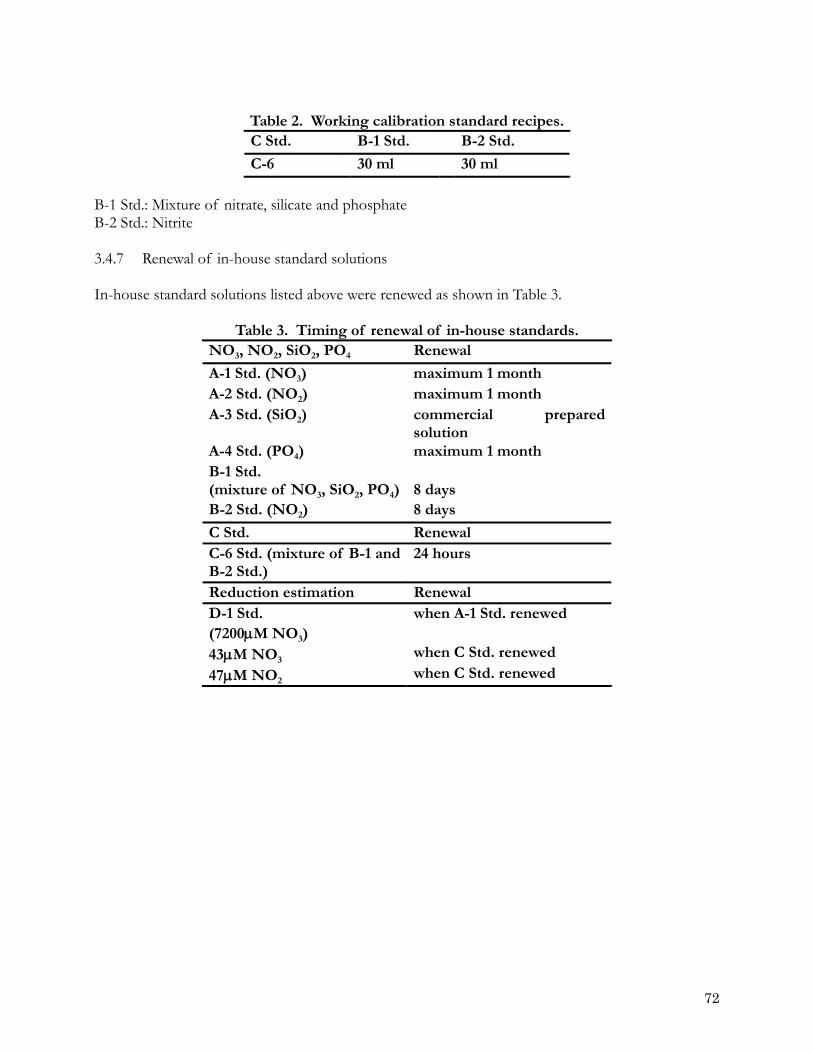
72

Table 2. Working calibration standard recipes. C Std. B-1 Std. B-2 Std.

C-6 30 ml 30 ml

B-1 Std.: Mixture of nitrate, silicate and phosphate B-2 Std.: Nitrite 3.4.7 Renewal of in-house standard solutions In-house standard solutions listed above were renewed as shown in Table 3.

Table 3. Timing of renewal of in-house standards. NO3, NO2, SiO2, PO4 Renewal

A-1 Std. (NO3) maximum 1 month A-2 Std. (NO2) maximum 1 month A-3 Std. (SiO2) commercial prepared

solution A-4 Std. (PO4) maximum 1 month B-1 Std. (mixture of NO3, SiO2, PO4) 8 days B-2 Std. (NO2) 8 days

C Std. Renewal C-6 Std. (mixture of B-1 and B-2 Std.)

24 hours

Reduction estimation Renewal D-1 Std. (7200μM NO3)

when A-1 Std. renewed

43μM NO3 when C Std. renewed

47μM NO2 when C Std. renewed

NSOP 10. PREPARATION OF CONTROL CHARTS 1. SCOPE AND FIELD OF APPLICATION This procedure details the preparation and use of property ( )X and range (R) control charts. The X chart is used to demonstrate whether a measurement mean is in control and the R chart is used to demonstrate whether measurement variability is in control. Such charts are basic tools for the quality assurance of analytical measurements. They can be used to document measurement uncertainty and to monitor a variety of aspects of a measurement process, such as blank levels or instrument sensitivity. 2. PRINCIPLE The construction of a control chart is based on statistical principles, specifically on the normal distribution. The control limits are based on considerations of probability, so that decisions that a system is in control are supported by evidence. Similarly, the control limits can be used to warn of potential problems and reveal the need for corrective action. Control charts should be kept in real time so that such corrective action is taken promptly. NSOP 11 provides all the necessary information to carry out the statistical calculations needed in this NSOP.

3. THE X CHART Values obtained for repetitive measurements of a control sample are plotted sequentially to evaluate the stability of the measurement process (see Figure 1). Such control samples must be similar to the test samples of interest, otherwise it is not possible to draw conclusions about the performance of the system on test samples from this information. The results from at least 12 measurements are needed to get the process underway (the temporal spread of the observations should be considered and chosen appropriately - limits can be set at the start of cruise based on experience from previous work)—are used to compute estimates of the mean and standard deviation of the data in accordance with the standard expressions given in NSOP 11.

73

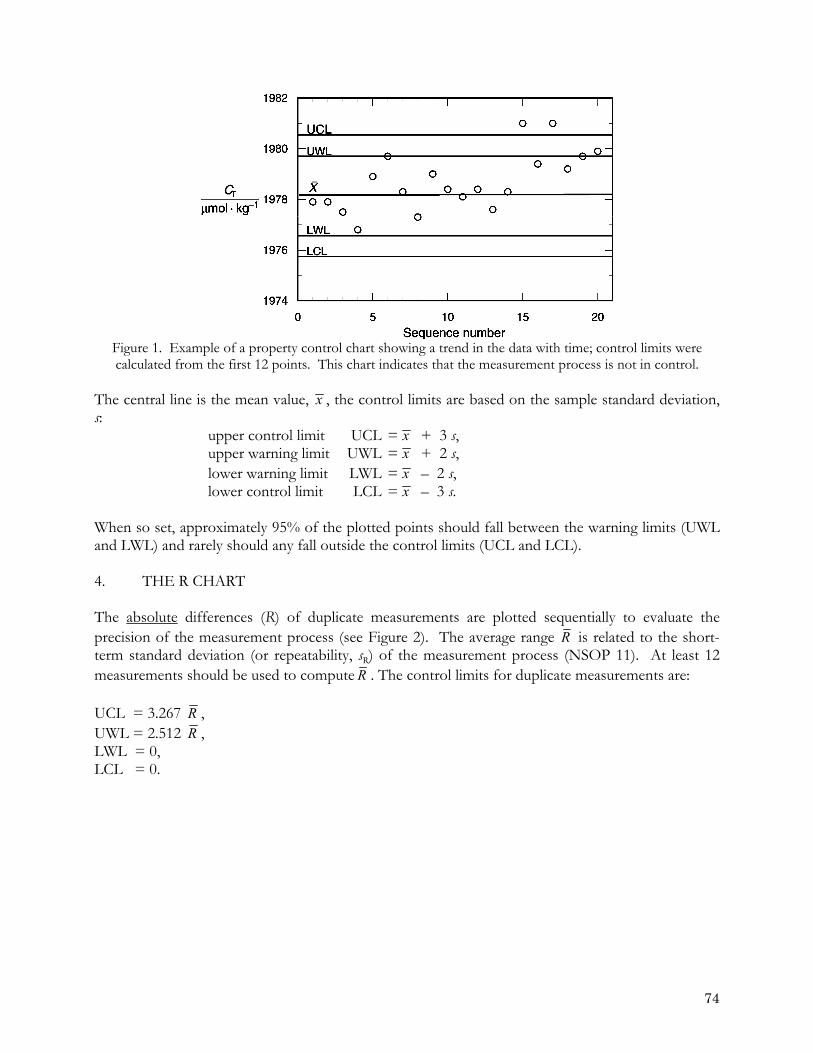
Figure 1. Example of a property control chart showing a trend in the data with time; control limits were calculated from the first 12 points. This chart indicates that the measurement process is not in control.

The central line is the mean value, x , the control limits are based on the sample standard deviation, s: upper control limit UCL = x + 3 s, upper warning limit UWL = x + 2 s, lower warning limit LWL = x – 2 s, lower control limit LCL = x – 3 s. When so set, approximately 95% of the plotted points should fall between the warning limits (UWL and LWL) and rarely should any fall outside the control limits (UCL and LCL). 4. THE R CHART The absolute differences (R) of duplicate measurements are plotted sequentially to evaluate the precision of the measurement process (see Figure 2). The average range R is related to the short-term standard deviation (or repeatability, sR) of the measurement process (NSOP 11). At least 12 measurements should be used to compute R . The control limits for duplicate measurements are: UCL = 3.267 R , UWL = 2.512 R , LWL = 0, LCL = 0.

74

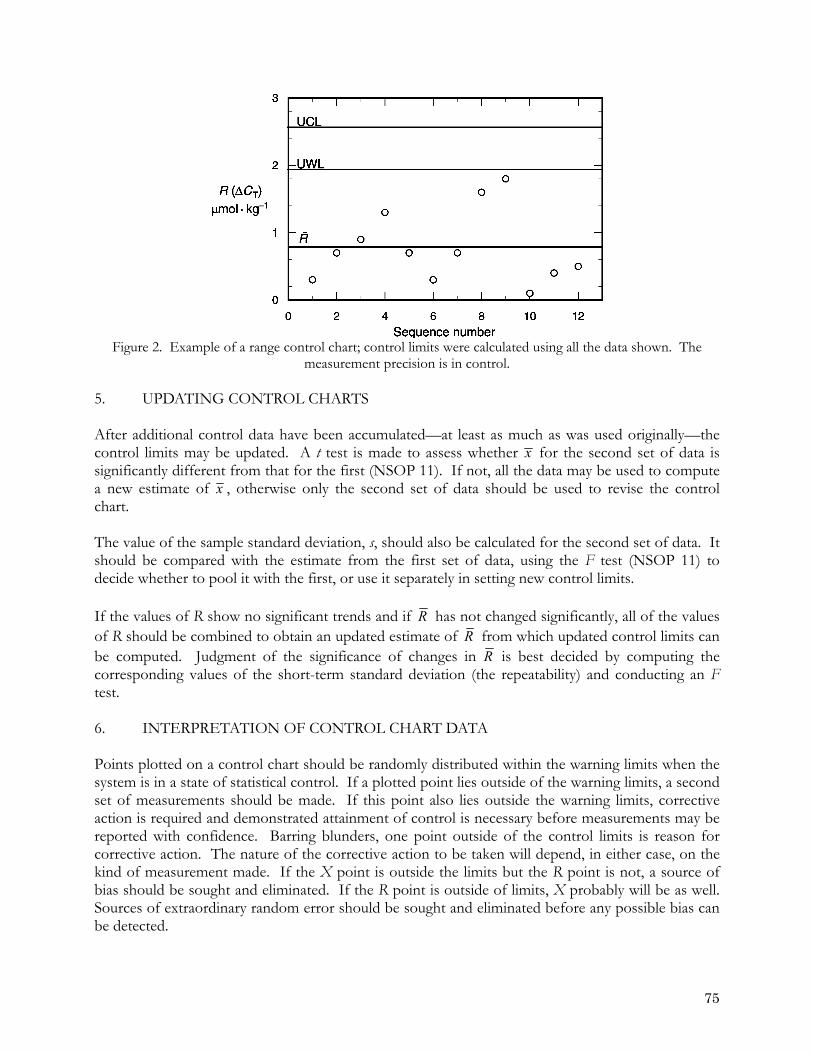
Figure 2. Example of a range control chart; control limits were calculated using all the data shown. The

measurement precision is in control. 5. UPDATING CONTROL CHARTS After additional control data have been accumulated—at least as much as was used originally—the control limits may be updated. A t test is made to assess whether x for the second set of data is significantly different from that for the first (NSOP 11). If not, all the data may be used to compute a new estimate of x , otherwise only the second set of data should be used to revise the control chart.

SOP 11) to ecide whether to pool it with the first, or use it separately in setting new control limits.

The value of the sample standard deviation, s, should also be calculated for the second set of data. It should be compared with the estimate from the first set of data, using the F test (Nd If the values of R show no significant trends and if R has not changed significantly, all of the values of R should be combined to obtain an updated estimate of R f m which updated control limits can be computed. Judgment of the significance of changes in

roR is best decided by computing the

corresponding values of the short-term standard deviation (the repeatability) and conducting an F st.

. INTERPRETATION OF CONTROL CHART DATA

traordinary random error should be sought and eliminated before any possible bias can

te 6 Points plotted on a control chart should be randomly distributed within the warning limits when the system is in a state of statistical control. If a plotted point lies outside of the warning limits, a second set of measurements should be made. If this point also lies outside the warning limits, corrective action is required and demonstrated attainment of control is necessary before measurements may be reported with confidence. Barring blunders, one point outside of the control limits is reason for corrective action. The nature of the corrective action to be taken will depend, in either case, on the kind of measurement made. If the X point is outside the limits but the R point is not, a source of bias should be sought and eliminated. If the R point is outside of limits, X probably will be as well. Sources of exbe detected.

75

76

Control charts may be used to evaluate the uncertainty of measurement in some cases. When an appropriate control chart is maintained, a X chart may be used to evaluate bias and to document the tandard deviation of the measurement process. Then the values of s on which the control limits are

g confidence limits for measurement values.

ateman, G. and Buydens, L. 1993. Quality Control in Analytical Chemistry, 2nd edition, Wiley-

aylor, J.K. and Oppermann, H.V. 1986. Handbook for the quality assurance of metrological measurements.

aylor, J.K. 1987. Quality Assurance of Chemical Measurements, Lewis Publishers, Inc., Chelsea,

Taylor, J.K. 1990. Statistical Techniques for Data Analysis. Lewis Publishers, Inc., Chelsea, 200 pp.

sbased may be used in calculatin 7. REFERENCES

KInterscience, New York, 317 pp.

Ryan, T.P. 1989. Statistical Methods for Quality Improvement. John Wiley & Sons, Inc., New York, 446 pp.

TNational Bureau of Standards. NBS Handbook 145.

T328 pp.

NSOP 11. STATISTICAL TECHNIQUES USED IN QUALITY ASSESSMENT 1. SCOPE AND FIELD OF APPLICATION NSOP 11, describes various statistical calculations used in quality assessment. Calculations are detailed which allow the computation of:-

• mean and standard deviation of a set of values • standard deviation from a set of duplicate measurements • confidence interval for a mean • examination of the values of two means or of two standard deviations to assess if they

are significantly different at some chosen level of probability • least-squares estimates of the slope and intercept of a straight line.

2. PRINCIPLE These calculations are based on statistical principles, specifically on the normal distribution. More details of the relevant statistical background are given in the bibliography. 3. PROCEDURE 3.1 Estimation of the mean and standard deviation from a series of measurements Given n measurements, 1 2 3, , , , nx x x xK , the mean, x , is given by

1

1 n

ii

x xn =

= ∑ (17)

and an estimate of the standard deviation, s, is given by

1 22

1

( )

1

n

ii

x xsn

=

⎛ ⎞−⎜ ⎟=

⎜ ⎟−⎝ ⎠

∑ .(18)

3.2 Estimation of the standard deviation from the difference of sets of duplicate measurements Given k differences of duplicate measurements, , 1 2 3, , , ,

kd d d dK

an estimate of the standard deviation, s, is given by

1 22

1

2

k

iR i

dsk

=

⎛ ⎞⎜ ⎟=⎜ ⎟⎝ ⎠

∑ . (19)

This is a measure of the short-term standard deviation, or repeatability of measurements6.

6 The International Organization for Standardization (ISO) applies two descriptions of precision: (1) the

reproducibility, the closeness of agreement between individual results obtained with the same method but under

77

3.3 Confidence interval for a mean The formula for use is

tsxn

± (20)

where x = sample mean,

n = number of measurements on which the mean is based, s = estimate of the standard deviation7, t = Student’s t value, i.e., the probability factor for the desired confidence limit and the

number of degrees of freedom associated with s. (For numerical values, see Table 1 in the Annexe to this procedure.) 3.4 Comparing values of two means Case 1. No reason to believe that the standard deviations differ. Step 1:Step 2:

Choose α, the desired probability level (i.e., the significance level) of the test. Calculate a pooled standard deviation from the two estimates to obtain a better estimate of

the standard deviation:

1 22 2

A A B Bp

A B

s ss ν νν ν

⎛ += ⎜ +⎝ ⎠

⎞⎟

Step 3:

(21)

where υA and υB are the number of degrees of freedom associated with sA and sB, respectively. sp will thus be based on υA + υB degrees of freedom.

Calculate the uncertainty, U, of the differences

1 2

pA B

1 1U tsn n

⎛= +⎜

⎝ ⎠

⎞⎟

Step 4:

(22)

where t is the appropriate Student’s t value. Compare A Bx xΔ = − with U. If Δ ≤ U, there is no reason to believe that the means

disagree. Case 2. The standard deviations differ significantly (see section 3.5). Step 1:Step 2:

Choose α, the significance level of the test. Compute the estimated variance of each mean using the individual estimates of the

standard deviations, 2

A A A B B B,V s n V s n= = 2

Step 3:

. (23) Compute the effective number of degrees of freedom8 :

different conditions (e.g., in different laboratories) and (2) the repeatability, the closeness of agreement between successive results obtained with the same method and under the same conditions.

7 If x and s are based on the same data set, the number of degrees of freedom, df = n – 1. However, if s is based on additional evidence, such as a system under statistical control (judged by a control chart), then the degrees of freedom on which the estimate of s is based may be used to determine t. In such a case, one can calculate a confidence interval for even a single measurement.

78

( )2A B

2 2A B

A B

* 2

1 1

V Vf V V

n n

+=

++ +

−

Step 4:

. (24)

Calculate the uncertainty, U, of the differences A B

*U t V V= + (25) where t* is the effective value of t based on f * degrees of freedom and the chosen

significance level, a (Table 1 in the Annex to this NSOP). Step 5: Compare A Ax xΔ = − with U. If Δ ≤ U, there is no reason to believe that the means

disagree. 3.5 Comparing estimates of a standard deviation (F test) This test may be used to decide whether there is sufficient reason to believe that two estimates of a standard deviation are significantly different. It consists of calculating the ratio of the variances and comparing it with tabulated values. Unless the computed ratio is larger than the tabulated value, there is no reason to believe that the respective standard deviations are significantly different. The F ratio is calculated as

2L2S

sFs

= (26)

where sL is the larger value and sS is the smaller of the two estimates under consideration. The critical value of F will depend on the significance level chosen and on the degrees of freedom associated with sL and sS (see Table 2 in the Annex to this NSOP). 3.6 Computation of least-squares estimates For the linear model, 0 1i iy x iβ β= + + ε (27) where x is essentially without error (for data with errors in x and y—see York, 1966) and the error εi is normally distributed with a constant variance, least- squares estimates of the coefficients, β0 and β1, are given by the expressions

1 2

( )(

( )

i ii

ii

)x x y y

x xβ

− −=

−

∑∑

, (28)

0 y 1xβ β= − . (29) An estimate of the experimental error variance is then given by

2

0 12

( )

2

i ii

y xs

n

β β− −=

−

∑ (30)

and estimates of the standard errors of the coefficients by

1 22

20

1S.E.( ) ( )i

i

xs n x xβ⎛ ⎞+⎜= −⎜⎝ ⎠

∑ ⎟⎟

, (31)

8 A number of expressions exist in the literature for this calculation, with some authors even arguing that such a

pooling of the variances is inappropriate. The expression used here comes from Taylor (1987).

79

( )1 1 2

2S.E.( )

( )ii

s

x xβ =

−∑. (32)

3.7 Example calculations 3.7.1 Estimation of the mean and standard deviation from a series of measurements Given the following 9 measurements: 1977.67, 1977.98, 1977.29, 1978.60, 1979.48, 1979.14, 1979.33, 1979.95, 1979.99, the mean is 1978.83 and the standard deviation is 0.99. 3.7.2 Estimation of the standard deviation from the difference of sets of duplicate measurements Given 10 pairs of measurements: 1976.8, 1979.3; 1978.9, 1979.6; 1979.6, 1979.8; 1978.3, 1978.6; 1981.2, 1979.8; 1977.6, 1977.8; 1976.2, 1976.8; 1978.6, 1977.0; 1976.6, 1978.9; 1978.3, 1978.9 the standard deviation calculated using

1 2

2

1

2

iiR

ds

k=

⎛ ⎞⎜ ⎟=⎜ ⎟⎝ ⎠

∑

is 0.93. 3.7.3 Confidence interval for a mean The 95% confidence interval for the mean calculated in section 3.7.1 is

(2.306)(0.99)1978.83 1978.83 0.769

± = ±

3.7.4 Comparing values for two means Case 1. No reason to believe that the standard deviations differ. A A1978.78, 0.93, 9x s= = An = B B1981.74, 0.87, 18x s n= = B =

Step 1:Step 2:

Require 95 % confidence in decision. Pooled standard deviation:

80

1 22 2

p8(0.93) 17(0.87)

8 170.89.

s⎛ ⎞+

= ⎜ ⎟+⎝ ⎠=

Step 3: Calculate U:

1 21 12.060(0.89)

9 180.75.

U ⎛ ⎞= +⎜ ⎟⎝ ⎠

=

Step 4: As ∆ (= 1981.74 – 1978.78 = 2.96) is larger than U, the means disagree at the 95 % confidence level.

Case 2. The standard deviations differ significantly.

A A1978.78, 0.93, 9x s= = An = B B1981.74, 2.75, 16x s n= = B =

Step 1:Step 2:

Step 3:

Require 95 % confidence in decision. Compute the estimated variance of each mean:

2

A2

B

(0.93) / 9 0.0961

(2.75) /16 0.4727.

V

V

= =

= =

Compute the effective number of degrees of freedom:

2

2 2* (0.0961 0.4727)

2 21.(0.0961) (9 1) (0.4727) (16 1)

f+⎡ ⎤= −⎢ ⎥+ + +⎣ ⎦

≈

Step 4:

Calculate U: 1 22.08(0.0961 0.4727) 1.57U = + = .

Step 5: As ∆ (= 1981.74 – 1978.78 = 2.96) is larger than U, the means disagree at the 95 % confidence level.

3.7.5 Comparing estimates of a standard deviation

A A1978.78, 0.93, 9x s= = An = B B1975.35, 1.71, 12x s n= = B =

Calculate F:

2

2

(1.71) 3.38(0.93)

F = = .

The tabulated value of F—with 8 degrees of freedom in the numerator and 11 degrees of freedom in the denominator—is 3.7. As the computed value is smaller than the tabulated value, there is no reason to believe that the two standard deviations are significantly different. 3.7.6 Example computation of least-squares estimates Given 6 pairs of measurements of x and y: 0.0 1892 498.8 66537

81

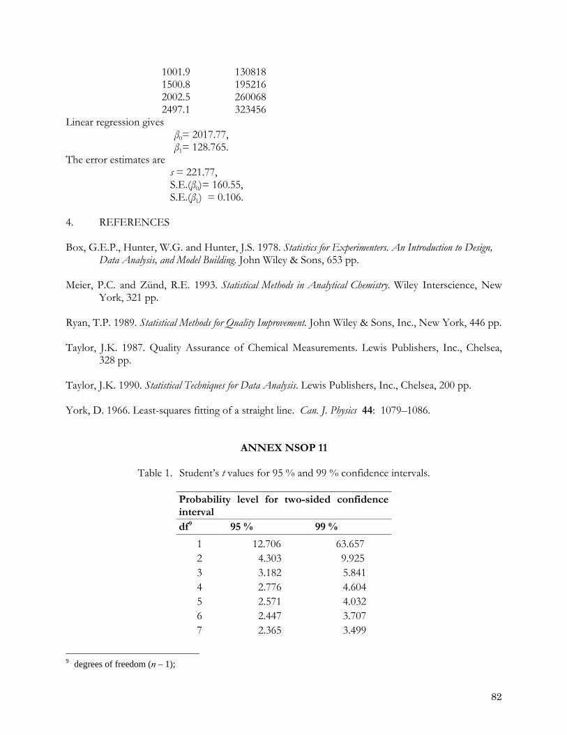
1001.9 130818 1500.8 195216 2002.5 260068 2497.1 323456 Linear regression gives

β0= 2017.77, β1= 128.765.

The error estimates are s = 221.77, S.E.(β0)= 160.55, S.E.(β1) = 0.106.

4. REFERENCES Box, G.E.P., Hunter, W.G. and Hunter, J.S. 1978. Statistics for Experimenters. An Introduction to Design,

Data Analysis, and Model Building. John Wiley & Sons, 653 pp. Meier, P.C. and Zünd, R.E. 1993. Statistical Methods in Analytical Chemistry. Wiley Interscience, New

York, 321 pp. Ryan, T.P. 1989. Statistical Methods for Quality Improvement. John Wiley & Sons, Inc., New York, 446 pp. Taylor, J.K. 1987. Quality Assurance of Chemical Measurements. Lewis Publishers, Inc., Chelsea,

328 pp. Taylor, J.K. 1990. Statistical Techniques for Data Analysis. Lewis Publishers, Inc., Chelsea, 200 pp. York, D. 1966. Least-squares fitting of a straight line. Can. J. Physics 44: 1079–1086.

ANNEX NSOP 11

Table 1. Student’s t values for 95 % and 99 % confidence intervals.

Probability level for two-sided confidence interval df9

95 % 99 %

1 12.706 63.657 2 4.303 9.925 3 3.182 5.841 4 2.776 4.604 5 2.571 4.032 6 2.447 3.707 7 2.365 3.499

9 degrees of freedom (n – 1);

82

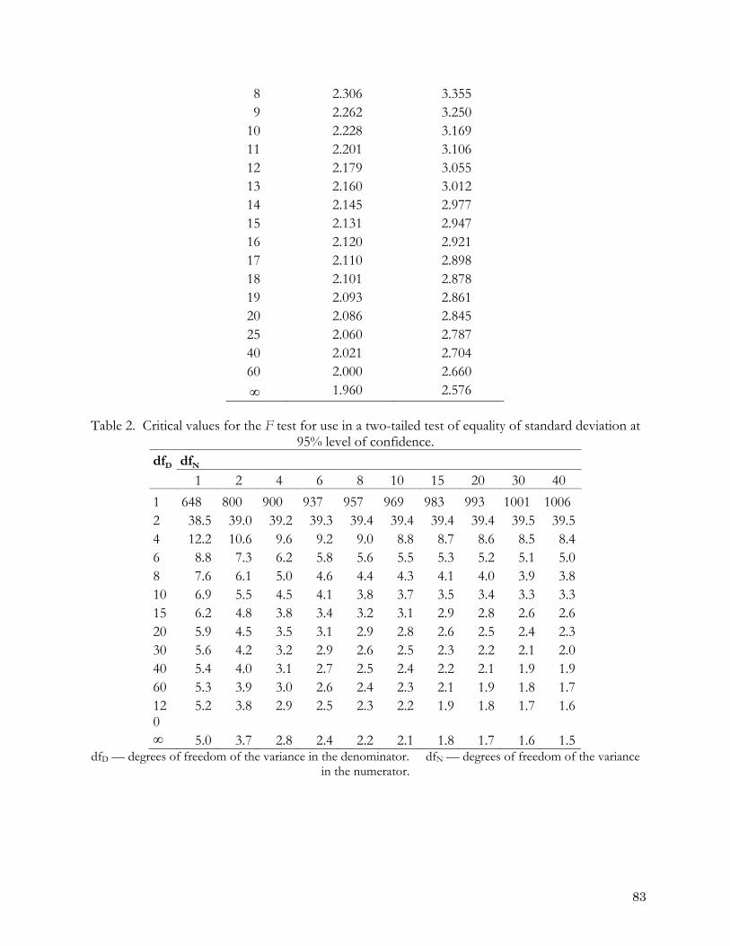
83

8 2.306 3.355 9 2.262 3.250 10 2.228 3.169 11 2.201 3.106 12 2.179 3.055 13 2.160 3.012 14 2.145 2.977 15 2.131 2.947 16 2.120 2.921 17 2.110 2.898 18 2.101 2.878 19 2.093 2.861 20 2.086 2.845 25 2.060 2.787 40 2.021 2.704 60 2.000 2.660 ∞ 1.960 2.576

Table 2. Critical values for the F test for use in a two-tailed test of equality of standard deviation at

95% level of confidence. dfD dfN

1 2 4 6 8 10 15 20 30 40 1 648 800 900 937 957 969 983 993 1001 1006 2 38.5 39.0 39.2 39.3 39.4 39.4 39.4 39.4 39.5 39.5 4 12.2 10.6 9.6 9.2 9.0 8.8 8.7 8.6 8.5 8.4 6 8.8 7.3 6.2 5.8 5.6 5.5 5.3 5.2 5.1 5.0 8 7.6 6.1 5.0 4.6 4.4 4.3 4.1 4.0 3.9 3.8 10 6.9 5.5 4.5 4.1 3.8 3.7 3.5 3.4 3.3 3.3 15 6.2 4.8 3.8 3.4 3.2 3.1 2.9 2.8 2.6 2.6 20 5.9 4.5 3.5 3.1 2.9 2.8 2.6 2.5 2.4 2.3 30 5.6 4.2 3.2 2.9 2.6 2.5 2.3 2.2 2.1 2.0 40 5.4 4.0 3.1 2.7 2.5 2.4 2.2 2.1 1.9 1.9 60 5.3 3.9 3.0 2.6 2.4 2.3 2.1 1.9 1.8 1.7 120

5.2 3.8 2.9 2.5 2.3 2.2 1.9 1.8 1.7 1.6

∞ 5.0 3.7 2.8 2.4 2.2 2.1 1.8 1.7 1.6 1.5 dfD — degrees of freedom of the variance in the denominator. dfN — degrees of freedom of the variance

in the numerator.

NSOP 12. REQUIREMENTS FOR REPORTING OF NUTRIENT META-DATA 1. SCOPE AND FIELD OF APPLICATION Reporting of a comprehensive meta-data set is an essential step required for the validation of data set within any data base it is entered into. An standard electronic form is being developed and will be made available to enable efficient and consistent reporting of meta-data across the global marine nutrient measurement community, an example is shown in Figure 12.1 below. 2. PRINCIPLE All nutrient data collected should be accompanied by a complete meta-data set which follows the requirements set out below. General Information: (this information is generic to all meta-data collected during a scientific cruise, and is needed to link data sets):

1. Cruise information: • Vessel (name; country; vessel ID) • Date and Port of departure • Date and Port of arrival • Cruise ID (EXPOCODE) • Name of experiment (e.g. P16 or M60/5) • Leg • Geographical coverage (e.g. North Atlantic; 30 °N to 50 °N and 60 °W to 10 °W) • Number of CTD stations

Nutrient measurements:

1. Investigator:

• Name: • Organization: • Address: • Phone: • Email:

2. Variables description: • Variable names • Reporting units

Method description:

Record 1. Instrument: State instrumentation used for the measurements. For instance: Braan-

Luebbe TrAAcs 800 autoanalyzer. 2. Method for each measured parameter, and appropriate reference. For instance:

Ammonium was measured with o-phthalaldehyde (OPA) in the presence of borate buffer

84

solution and sodium sulfite; fluorescence measured at 460 nm, excitation at 370 nm. Method no G-327-05 Rev 3 (Seal Analytics), Kerouel and Aminot, 1997.

3. Deviations in your set-up from the reference method. 4. Modifications to the standard instrument configuration for the method 5. Settings such as the sampling/rinsing cycles, temperatures, air/nitrogen in the gas

bubbles etc 6. Lab temperature (e.g. 20-24°C variable). 7. Sampling containers type (e.g. 100 ml polypropylene bottles, reused after acid clean). 8. Any preprocessing of sample (e.g filtration - record filter type and method used pressure

or suction etc.) 9. Poisoning of samples? 10. Storage – method used and duration (e.g. frozen -20 oC for three months defrosted 3

days before measurement) 11. Thawing procedures if sample was frozen

Reagents:

1. Brands and stock information of the reagents/salts used. 2. Where the solutions prepared on the ship, or pre-made in the lab prior to cruise 3. Which medium was used for the reagents (e.g. RO water)

Standardization:

1. How were your stock solutions prepared (initial salts, medium) 2. Temperature of preparation of standards (This is the temperature used when converting

µM l-1 to µM kg-1) 3. Dilution sequence used to prepare working standards 4. Medium used for working standards 5. Blank measurements (medium) 6. Pipettes were used and calibration history

Reference material:

1. Certified reference material or certified standards used (state batch numbers, producer etc.).

Quantification procedures:

1. Software used for peak picking and calibration 2. Degree of equation used for calibration and zero forced through origin 3. Calibration curves/ranges (number of points used for calibration curve, concentration

used for calibrants) 4. Blank corrections (Null and refractive index blank) 5. Matrix corrections (method used to quantify corrections)

Data quality:

85

1. Estimate of accuracy10 and precision11. 2. State how these numbers were obtained (e.g. by measurements of X duplicates and by

running X number of Certified Reference Material). 3. Proportion of samples measured in duplicate 4. Method used to round off results to the number of significant digits

Samples results:

1. Header file showing what was measured (variables/parameters, units); 2. Time and location of sample taken(time; latitude; longitude; station identifier) 3. Time sample was measured 4. Raw nutrient data 5. Nutrient data adjusted for tracking and RMNS results 6. Clear statement that the data are reported as µM l-1 or µM kg-1

3. NOTES A significant part of the information required above is specific for the nutrient measurements. Several of these fields will be generic for a particular lab, i.e. will only have to filled out once by each lab; variations to the standard procedures then be edited in along with specific information for each cruise such as the precision data. Figure 1 (below) shows an example of the electronic (pdf based) meta-data reporting form that will be made available by the RMNS project for use by the global community reporting data on concentrations of nutrients in the ocean.

10 “Accuracy" is the closeness of agreement between a measured value and the true quantitative value of the measurand. It can only be quantified in situations where measurements can be made of a measurand for which an agreed value exists such as a certified reference material. 11 “Precision” is the closeness of agreement of replicate measurements of the same property under specified conditions. It can be quantified by a measure such as standard deviation. Definitions follow VIM (International Vocabulary of Metrology); http://www.bipm.org/utils/common/documents/jcgm/JCGM_200_2008.pdf

86

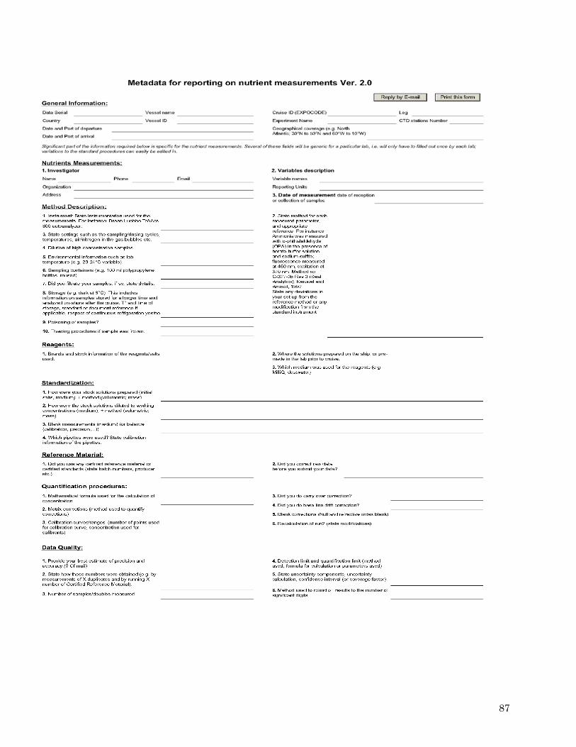
87