Determination of frequency and temperature dependent ... · PDF fileDetermination of frequency and temperature dependent mechanical material properties by ... are used for the calculation

Determination of frequency and temperature dependent mechanical material properties by means of an Inverse Method

J. Ilg, S. J. Rupitsch & R. Lerch Chair of Sensor Technology, Friedrich-Alexander-University, Erlangen-Nuremberg, Germany

Abstract

We present a method to determine the frequency as well as the temperature dependence of mechanical material parameters. In general, we apply a so-called Inverse Method that adapts simulation results to match the best possible measurements. The variable quantities within the simulation are the sought-after material parameters, namely the elasticity modulus, Poisson’s ratio, and a damping factor. Measurements are carried out by applying forced mechanical vibrations over a wide frequency range from quasi static up to more than 5 kHz. In particular, an electromechanical shaker harmonically excites tensile or bending vibrations of clamped plates and cylindrically shaped specimens. Two Laser Doppler vibrometers measure the vibration right next to the clamping and at the free end of the specimen, yielding a frequency dependent transfer function by relating the two measurands. Since the experimental setup is built up within an environmental chamber, temperatures from -40 to 150°C can be applied. Based on the experiment and the actual measuring points, a finite element (FE) analysis is performed to simulate the transfer function. Finally, the Inverse Method iteratively adapts the sought-after material parameters in such a convenient way that the simulated transfer function matches the measured one. The presented method was utilized to investigate the frequency and temperature dependence of different material classes: silicon rubber, plastics, metals, ceramics, and glass fibre reinforced plastics. In order to quantify and compare the dynamic material behaviour, functional relations of elasticity modulus/damping factor versus temperature are determined. Keywords: elasticity modulus, damping factor, forced vibration testing, frequency dependence, temperature dependence, mechanical material properties.

Materials Characterisation VI 101

www.witpress.com, ISSN 1743-3533 (on-line) WIT Transactions on Engineering Sciences, Vol 77, © 2013 WIT Press

doi:10.2495/MC130091

1 Introduction

The development and design of every technical device demands for reliable material parameters of all involved materials. First and foremost, the parameters are used for the calculation of the structural capability. Furthermore, the increasing usage of computer aided engineering requests precise material parameters. Especially for sensors and actuators, an exact knowledge of mechanical as well as electrical quantities yields reliable simulations and ensures the functionality of a device. For the identification of the material parameters of piezoceramic transducers, we already introduced a so-called Inverse Method [1, 2]. Based on this method, the present contribution deals with a similar procedure to investigate the dynamic as well as thermal dependencies of mechanical material properties, namely elasticity modulus, Poisson’s ratio, and a damping factor. In most cases, the mechanical properties for a material – e.g. provided by the manufacturer – are given as static values, typically arising from tensile or bending tests. Other possible methods are the indentation of defined tips and the acoustical logging of ultrasound pulses. It is well known that material properties more or less depend on temperature and frequency. Moreover, the so-called Williams-Landel-Ferry (WLF) shift constant gives a nonlinear relation between these two dependencies [3]. Especially plastics show a significant sensitivity due to frequency and temperature. Consequently, many applications could benefit from a more precise knowledge of these relations. Some publications already dealt with this topic, mostly by exciting a specimen with a defined force and calculating material parameters with analytical descriptions (e.g., [4, 5]). Although these approaches exhibit very short computing times, they are exclusively applicable to specific sample geometries and demand for well defined experimental setups. Just as other research [6, 7], we overcome this problem by means of using finite element simulations instead of analytical relations. In principle, these methods allow for arbitrary sample geometries und various measurements quantities at the cost of computational effort. In contrast to the existing publications on this topic, our novel method mainly benefits from utilizing both, a proven and tested optimization algorithm as well as an adapted finite element method. In addition, the experimental setup covers a wider frequency and temperature range compared to previous researches. Our first approach for determining frequency dependent material parameters was published in [8, 9] applied to cylindrically shaped specimens made of silicone rubber. The present paper mainly deals with thin-walled components, namely polymer, ceramic, and aluminium plates. The paper is organized as follows: In Sec. 2 the experimental setup to measured frequency resolved transfer function is explained. The utilized FE model and approach is briefly discussed in Sec. 3. After these fundamentals, the applied Inverse Method to determine frequency dependent material properties is described with different sub-steps (Sec. 4). Section 5 gives examples of possible investigations with the presented method and lists the results. Finally, the paper is summarized in Sec. 6, including a short outlook to our future research.

102 Materials Characterisation VI


2 Experimental setup

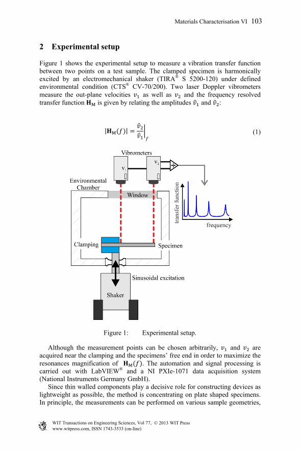
Figure 1 shows the experimental setup to measure a vibration transfer function between two points on a test sample. The clamped specimen is harmonically excited by an electromechanical shaker (TIRA® S 5200-120) under defined environmental condition (CTS® CV-70/200). Two laser Doppler vibrometers measure the out-plane velocities as well as and the frequency resolved transfer function M is given by relating the amplitudes and :

| M | (1)

Figure 1: Experimental setup.

Although the measurement points can be chosen arbitrarily, and are acquired near the clamping and the specimens’ free end in order to maximize the resonances magnification of M . The automation and signal processing is carried out with LabVIEW® and a NI PXIe-1071 data acquisition system (National Instruments Germany GmbH). Since thin walled components play a decisive role for constructing devices as lightweight as possible, the method is concentrating on plate shaped specimens. In principle, the measurements can be performed on various sample geometries,



though it fits especially to rotationally symmetric specimens as the computational effort (Sec. 3) can be reduced in this case [8, 9]. Figure 2 displays the three different possible excitations of a clamped beam in single direction: bending around x-axis (a), bending around z-axis (b), tension in y-direction (c). Cylindrically shaped samples are exclusively excited in z-direction (d). Note that the definition of the coordinate system is given in Fig. 3 and is always related to the specimen. One major problem, especially for the cases (b) and (c), is the occurrence of undesired vibrations in other directions than movement of the shakers base. The mass centre of clamping and sample do not exactly coincide with the shakers axis for various specimens. This results in an increasingly swaying movement of the shakers base and especially the free end of the sample for higher frequencies. In order to exclusively measure the vibration in the direction of the excitation , an in-plane laser Doppler vibrometer is utilized (Polytec® LSV-065-306F). Velocity is always detected by means of an out-of-plane vibrometer (Polytec® OFV-303) that measures the surface normal velocity. The type of vibrometer is indicated with a double-pointed arrow in Fig. 2.

Figure 2: Different cases of excitation for the two sample geometries: bending of a plate over short edge (a) and long edge (b), tension of a plate (c), tension of a cylinder (d); v1 and v2 represent the two measurands.

The measurement procedure is organized as follows: At first, the desired temperature is committed to the chamber control and the actual temperature is measured by means of a PT100 near to the free end of the sample. When this sensor detects the achievement of the target temperature, a holding time of 30 minutes is applied to ensure a homogeneous temperature distribution within the specimen. Subsequent, the transfer function is acquired by measuring and

for each entry in a given frequency vector. Note that these amplitudes are calculated by averaging over 100 single sinusoidal vibrations. The limitation of the frequency range depends on various quantities. First, the whole shaker setup exhibits resonance frequencies as well, depending on the masses of plunger,



clamping, and specimen (manufacturer data for unloaded base: >5 kHz). Consequently, the input power to the shaker has to be increased when the first anti-resonance occurs to provide a significant movement of the clamping. Second, the vibrometers introduce some limitations, namely a lower frequency limit and a specific sensitivity that determines the possible resolution of the measurements. Typically the frequency range is limited to 10 Hz – 5 kHz, but especially for materials with a low damping factor, measurements could be carried out up to more than 10 kHz (see Sec. 5).

3 Finite element models

Additionally to the measurements, the presented Inverse Method is based on FE simulations. Therefore, a finite element model is needed that fulfils both, precise simulation results as well as minimum computing time. For the standard FE method (h–version) based on finite elements with second order shape functions the aspect ratio of an element is limited to avoid locking effects (see e.g. [10]). Since mainly thin walled samples are investigated, this standard method would result in a high amount of elements and as a consequence in high computing times. On account of this fact, the presented method uses FE models with hierarchic shape functions (p–version) of higher order (p > 2). Additionally, the utilized non-commercial FE tool CFS++ [11] allows for the implementation of anisotropic shape functions – here, the order in x- and y-direction is chosen higher than along the thickness. For detailed information on this topic, we refer to [12– 14]. The order p of the shape functions is chosen by means of increasing p until the simulated transfer function converges towards the solution with a very fine standard FE mesh. Note that for this parameter study, the transfer function contains five resonances. An example of a FE model optimized for the –version is given in Fig. 3 (left). In case of cylindrical specimens the standard h–version with second order shape functions is applied and the resulting model is exemplarily displayed in the right drawing of Fig. 3.

Figure 3: Finite element models for a plate shaped specimen (left) and for a cylindrical sample (right).

The simulated frequency resolved transfer function S is calculated equally to the measured one (Eq. (1)). For a plate, the nodes at the bottom and



the top side – with respect to z-direction – between the clamping are harmonically excited in one direction and fixed in the others. The excitation for cylindrical models is defined corresponding to the applied clamping as well (compare Figs. 2 and 3). The material of the FE models is assumed to be globally homogeneous and isotropic. The variable material parameters are the real part of the elasticity modulus , the damping factor , and the Poisson’s ratio . Typically, the complex Young’s modulus is given by

j (2)

and the damping factor or loss factor tan is defined by the quotient between imaginary and real part :

2 tan (3)

Note that due to readability, the real part of the elasticity modulus is denoted as . Considering the three different cases of excitation (Fig. 2),

corresponds to the bending/flexural modulus or a tensile modulus. Only in case of isotropic material samples, represents the Young’s modulus.

4 Inverse Method

The presented measurements und FE models are necessary input quantities for the so-called Inverse Method. This procedure is implemented in MATLAB® (The MathWorks, Inc.) and can be divided into the three sub-steps described in the following. Additionally, the result of each step is given in Fig. 4. Within every step, one or more material parameters are adapted in order fit simulation results towards the measurements.

4.1 Eigenfrequency optimization

At first, the elasticity modulus is adapted by means of two eigenfrequency simulations and the measured resonance frequencies that can be obtained from the measured transfer function. Based on the difference between two simulated eigenfrequencies S, S, with respect to a given variation of the moduli

, a proper initial guess , for the n-th eigenfrequency M, is calculated by assuming proportionality. This first step provides the following optimization with a proper initial guess of for every resonance (see Fig. 4) that was found in the measured transfer function. The major benefit of this preliminary step is that the whole procedure can start with a completely unknown set of material parameters.



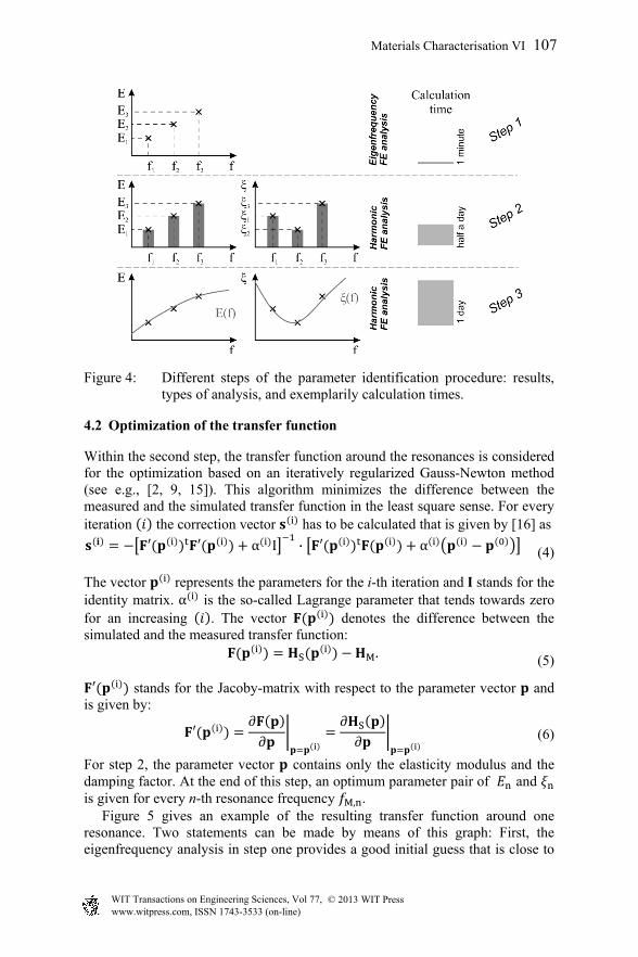
Figure 4: Different steps of the parameter identification procedure: results, types of analysis, and exemplarily calculation times.

4.2 Optimization of the transfer function

Within the second step, the transfer function around the resonances is considered for the optimization based on an iteratively regularized Gauss-Newton method (see e.g., [2, 9, 15]). This algorithm minimizes the difference between the measured and the simulated transfer function in the least square sense. For every iteration the correction vector has to be calculated that is given by [16] as

α I · α (4)

The vector represents the parameters for the i-th iteration and stands for the identity matrix. α is the so-called Lagrange parameter that tends towards zero for an increasing . The vector denotes the difference between the simulated and the measured transfer function:

S M. (5)

stands for the Jacoby-matrix with respect to the parameter vector and is given by:

∂∂

∂ S

∂ (6)

For step 2, the parameter vector contains only the elasticity modulus and the damping factor. At the end of this step, an optimum parameter pair of and is given for every n-th resonance frequency M, . Figure 5 gives an example of the resulting transfer function around one resonance. Two statements can be made by means of this graph: First, the eigenfrequency analysis in step one provides a good initial guess that is close to



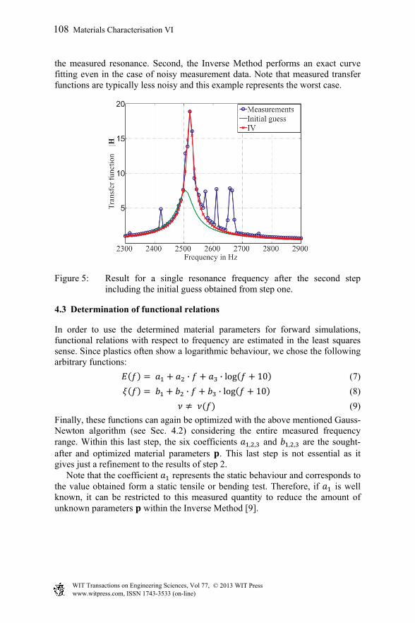
the measured resonance. Second, the Inverse Method performs an exact curve fitting even in the case of noisy measurement data. Note that measured transfer functions are typically less noisy and this example represents the worst case.

Figure 5: Result for a single resonance frequency after the second step including the initial guess obtained from step one.

4.3 Determination of functional relations

In order to use the determined material parameters for forward simulations, functional relations with respect to frequency are estimated in the least squares sense. Since plastics often show a logarithmic behaviour, we chose the following arbitrary functions:

· · log 10

· · log 10

(7)

(8)

(9)

Finally, these functions can again be optimized with the above mentioned Gauss-Newton algorithm (see Sec. 4.2) considering the entire measured frequency range. Within this last step, the six coefficients , , and , , are the sought-after and optimized material parameters . This last step is not essential as it gives just a refinement to the results of step 2. Note that the coefficient represents the static behaviour and corresponds to the value obtained form a static tensile or bending test. Therefore, if is well known, it can be restricted to this measured quantity to reduce the amount of unknown parameters within the Inverse Method [9].



5 Results

This section gives examples of measurements that can be carried out with the presented experimental setup and the Inverse Method. First, Fig. 6 shows the temperature dependent bending modules of a high-pressure die-casted aluminium plate identified with excitation case (a) (see Fig. 2). Here, the results are obtained only from the first step of the Inverse Method. Although, the accuracy of the determined elasticity modulus depends on the frequency resolution, a good indication of the temperature dependence is given.

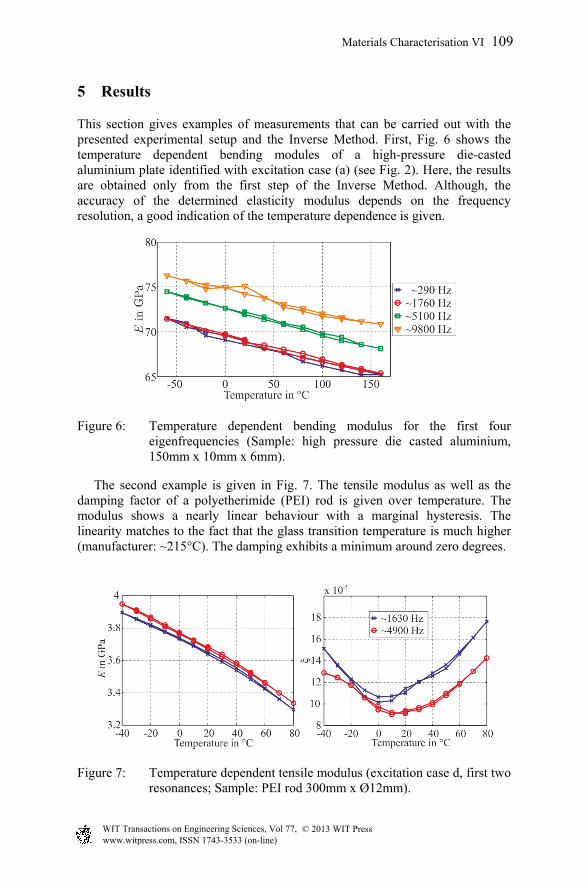
Figure 6: Temperature dependent bending modulus for the first four eigenfrequencies (Sample: high pressure die casted aluminium, 150mm x 10mm x 6mm).

The second example is given in Fig. 7. The tensile modulus as well as the damping factor of a polyetherimide (PEI) rod is given over temperature. The modulus shows a nearly linear behaviour with a marginal hysteresis. The linearity matches to the fact that the glass transition temperature is much higher (manufacturer: ~215°C). The damping exhibits a minimum around zero degrees.

Figure 7: Temperature dependent tensile modulus (excitation case d, first two resonances; Sample: PEI rod 300mm x Ø12mm).



The last example is given in Fig. 8, investigating a glass fibre reinforced polypropylene (GFR-PP) plate. Here, the frequency dependent bending modulus is given for different temperatures. One can see that with increasing temperature, the modulus is decreasing much more with frequency. The glass transition temperature of PP is around 0°C, which can be observed in the wide distance to the -20°C and +20°C curves.

Figure 8: Frequency dependent bending modulus (excitation case a) for different temperatures (Sample: glass fibre reinforced polypropylene, TEPEX® dynalite104 2mm).

Finally, the frequency dependence of the material properties is quantitatively expressed according to Section 4.3. The determined coefficients of functional relations for various investigated materials are summarized in Tab. 1. The value

indicates the upper frequency limit of the measurements and consequently gives the range in which the functions are valid.

Table 1: Coefficients of the functional relations (Eqs (4) and (5)) for various investigated specimens, representing the bending modulus (case a) at room temperature (20°C).

(Pa) (Pa·s) (Pa) (s) PEI 3.08·109 -4.85·104 1.21·108 7.11·10-2 1.31·10-5 -2.51·10-2 GFR-PP 1.74·1010 1.44·104 4.09·108 3.20·10-2 -2.37·10-6 -6.20·10-3 Aluminium 6.83·1010 6.08·105 2.05·108 2.90·10-3 6.90·10-8 -7.21·10-4 ~ length width thickness PEI 2.5 kHz 280 mm 40 mm 5 mm GFR-PP 3.0 kHz 200 mm 40 mm 2 mm Aluminium 10.0 kHz 150 mm 10 mm 6 mm



6 Conclusion and outlook

We presented a novel method to determine the frequency as well as temperature dependence of the elasticity modulus and a damping factor. The experimental setup allows for dynamic bending and tensile loading of plate shaped specimens. In addition, the necessary finite element model is capable of producing reliable simulation results for thin-walled samples by applying the –version of the FE method. Both simulations and measurements are the input quantities for the utilized Inverse Method, wherein simulation results are adapted appropriately to match the experimental data. The determined material properties are quantified as functional relations versus frequency at room temperature for different specimens. The thermal dependencies of the elasticity modulus and the damping factor are graphically presented in different ways considering a single frequency or the whole frequency range. The investigated materials exhibit a more or less distinct frequency and temperature dependence. Especially for polymers – as one could expect – the dynamic and thermal properties have to be considered with a view to an accurate design of devices incorporating these materials. However, also aluminium shows a significant frequency and particularly temperature dependence. Well knowledge of both relations yields reliable simulation results and can help to reduce the weight of a device in a very early stage of development. The focus of our future work lies on including Poisson’s ratio in the Inverse Method and, furthermore, concentrating on transversally isotropic materials.

Acknowledgements

This research is supported by the Deutsche Forschungsgemeinschaft (DFG) in context of the Collaborative Research Centre/Transregio 39 PT-PIESA, subproject C6.

References

[1] Rupitsch, S. J. and Lerch, R.: Inverse Method to estimate material parameters for piezoceramic disc actuators. Applied Physics A, 97(4), pp. 735–740, 2009.

[2] Rupitsch, S.J., Ilg, J., Lerch, R., Enhancement of the Inverse Method Enabling the Material Parameter Identification for Piezoceramics. Proceedings of the IEEE Ultrasonic Symposium, Orlando, pp. 357–360, 2011.

[3] Ferry, J., Viscoelastic Properties of Polymers. Wiley-Interscience: Chichester, England, 1980.

[4] Madigosky, W.M. and Lee, G.F., Improved resonance technique for materials characterization. The Journal of the Acoustical Society of America, 73(4), pp. 1374–1377, 1983.



[5] Gibson, R.F., Modal vibration response measurements for characterization of composite materials and structures. Composites Science and Technology, 60(15), pp. 2769–2780, 2000.

[6] Willis, R.L., Lei Wu, L. and Berthelot, Y.H., Determination of the complex Young and shear dynamic moduli of viscoelastic materials. The Journal of the Acoustical Society of America, 109(2), pp. 611–621, 2001.

[7] Kim, S.-Y. and Lee, D.-H., Identification of fractional-derivative-model parameters of viscoelastic materials from measured FRFs. Journal of Sound and Vibration. 2009, 324(3-5), pp. 570–586.

[8] Ilg, J., Rupitsch, S.J., Sutor, A. and Lerch, R., Determination of Dynamic Material Properties of Silicone Rubber Using One-Point Measurements and Finite Element Simulations. IEEE Transactions on Instrumentation and Measurement, 61(11), pp. 3031–3038, 2012.

[9] Rupitsch, S.J., Ilg, J., Sutor, A., Lerch, R. and Döllinger, M., Simulation based estimation of dynamic mechanical properties for viscoelastic materials used for vocal fold models. Journal of Sound and Vibration, 330, pp. 4447–4459, 2011.

[10] Bathe, K.-J., Finite Element Procedures. Prentice Hall: New Jersey, 1996. [11] Kaltenbacher, M., Advanced Simulation Tool for the Design of Sensors and

Actuators. Proceedings Eurosensors XXIV, 5, pp. 597–600, 2010. [12] Duester, A., Broeker, H. and Rank, E., The p-version of the finite element

method for three-dimensional curved thin walled structures. Int. Journal for Numerical Methods in Engineering, 52, pp. 673–703, 2001.

[13] Šolín, P., Segeth, K. and Doležel, I., Higher-Order Finite Element Methods. Chapman and Hall: New York, 2004.

[14] Hauck, A., Kaltenbacher, M. and Lerch, R., Simulation of Thin Piezoelectric Structures Using Anisotropic Hierarchic Finite Elements. Proceedings of the IEEE Ultrasonics Symposium, Vancouver, pp. 476–479, 2006.

[15] Kaltenbacher, B., Neubauer, A. and Scherzer, O., Iterative Regularization Methods for Nonlinear Ill-Posed Problems. de Gruyter: Berlin New York, 2008.

[16] Rupitsch, S.J., Wolf, F., Sutor, A. and Lerch, R., Reliable modeling of piezoceramic materials utilized in sensors and actuators. Acta Mechanica, 223(8), pp. 1809–1821, 2012.



Documents

Determination of frequency and temperature dependent ... · PDF fileDetermination of frequency and temperature dependent mechanical material properties by ... are used for the calculation