DETERMINATION OF MIXING LENGTHS IN DILUTION GAUGING

A. BARSBY

Water Research Association Medmenham, Buckinghamshire, England

SUMMARY

Dilution gauging of river discharge depends on the injected tracer becoming adequately mixed with the flow, before samples are taken to assess the downstream concentration. However, as dispersion along a needlessly great mixing length demands the use of excessive time and tracer, it is important, prior to the dilution measurement, to determine the minimum length of river that will provide adequate mixing.

Alternative approaches to mixing length assessment are: (a) Calculation from channel and flow parameters, and (b) Observation of the dispersion of a preliminary injection. New studies in natural

streams are presented which provide an intercomparison of these techniques.

Constant rate injections have been used in a series of 9 tests the discharges ranging from 0.05 to 5 m3/sec. At several stations along each stream, mixing progress was observed by measuring the variation in concentration from bank to bank.

By using logarithmic interpolation of observed mixing at each station, deduced lengths for 99% mixing have been compared with results given by the empirical formulae of Hull, Rimmar, and André. The most satisfactory of these was Rimmar's and a modification of his formula is suggested, permitting evaluation of mixing lengths from easily measured parameters.

Sayre's equation, for lateral dispersion in a finite channel, has been developed to provide a simple technique of extrapolating from the length giving a measured degree of mixing to that required for mixing to the 99% level. Accordingly, preliminary injection experiments can be conducted over a small fraction of the eventual mixing length.

Techniques for reducing mixing lengths are discussed but a limitation to such improvement is pointed out and illustrated by an example of transversally-distributed multi-point injection.

The work confirms techniques (a) and (b) as complementary ones in the estimation of mixing length. Generally, calculation from channel parameters seems preferable in small turbulent streams, where a conservative estimate would be tolerable; the preli­minary injection method if recommended for larger rivers where accuracy of prediction justifies the additional work involved.

RESUME

Le calibrage de la dilution du débit de rivière dépend de ce que l'indicateur une fois injecté se mélange adéquatement avec le courant, avant que l'on puisse prendre des spécimens pour déterminer la concentration du courant dans le sens de l'aval. Toutefois, puisque la dispersion le long d'un bief de mélange pas nécessairement grand prend beaucoup de temps et demande l'emploi d'un indicateur, il est important avant de mesurer la dilution de déterminer le bief minimal qui fournira un mélange adéquat.

Il y a deux moyens alternatifs pour l'estimation de la longueur de mélange: a) Calculer au moyen de paramètres de canal et de courant; b) Observer la dispersion d'une injection préliminaire. On donne ici de nouvelles études

faites dans des cours d'eau naturels et qui fourniront une intercomparaison de ces techniques.

Des injections à taux constant ont été accomplies dans une série de 9 expériences, les débits allant de 0,05 à 5 m3 par seconde. En plusieurs endroits le long de chaque cours d'eau, on a observé les progrès de mélange en mesurant la variation de concen­tration d'une rive à l'autre.

En se servant d'interpolation logarithmique du mélange observé à chaque étape on a comparé les longueurs obtenues pour un mélange à 99% avec les résultats donnés par

395

les formules empiriques de Hull, Rimmar et André. De ces formules, la plus satisfaisante était celle de Rimmar et l'on en suggère une modification permettant l'évaluation des longueurs de mélange au moyen de paramètres faciles à mesurer.

L'équation de Sayre, pour la dispersion latérale dans un canal limité, a été dévelop­pée pour fournir une technique simple d'extrapoler à partir de la longueur donnant un degré mesuré de mélange jusqu'à la longueur nécessaire pour un mélange à un niveau de 99%. En conséquence on peut conduire des expériences d'injection préliminaires sur une petite fraction de la longueur finale de mélange.

Des techniques pour réduire les longueurs de mélange sont en discussion mais il faut faire remarquer qu'un tel perfectionnement a une limite qui s'illustre par un exemple d'injection à plusieurs points avec distribution transverse.

Les travaux confirment les techniques a) et b) comme complémentaires à l'estima­tion de la longueur de mélange. Le calcul au moyen de paramètres de canal semble généralement préférable dans les petits cours d'eau torrentiels où une évaluation modérée est suffisante. La méthode de l'injection préliminaire est recommandée pour les plus grandes rivières où l'exactitude des prédictions justifie le travail qu'elle entraîne en surcroît.

INTRODUCTION

The dilution method of river gauging depends on the assessment of the degree of dilution experienced by a tracer injected into the stream. A basic requirement of the method is that the determination of the diluted concentration shall be made at a station sufficiently far downstream of the injection point for adequate mixing with the river flow to have taken place. Although it is possible to sample at a station even further downstream, to do so would be extravagant of time and of tracer, and would accentuate the effect of any loss or degradation of the tracer. It is therefore an important prelimina­ry to a dilution gauging measurement to assess the minimum distance that will provide adequate mixing.

This paper presents experimental data from natural rivers, together with a theoreti­cal assessment of two techniques for the estimation of mixing lengths:

(a) The substitution of observed values of certain channel and flow parameters, such as depth, breadth, mean velocity etc., into one of several available empirical formulae, or

(b) The use, prior to the dilution gauging, of a trial injection in which the progress of mixing at several downstream stations is observed. Subsequently a value of the mixing length may be obtained by interpolation.

Field trials have been made to provide an intercomparison of these techniques and in particular to assess the reliability of each of the available formulae for mixing length prediction.

2. FIELD PROCEDURE TO DETERMINE PROGRESS OF MIXING

Nine field trials were carried out on rivers of widely differing character, with discharges ranging from 0.05 to 5 m3/sec. Tracer, either sodium or potassium chloride, was injected at the centre-point of each stream, at a constant rate. Between 3 and 6 sampling stations were employed, located downstream of the injection point at inter­vals providing roughly equal increments of mixing between successive stations. Sampling racks containing between 5 and 15 bottles equally spaced across the section were used for sampling the flow. The variation of concentration at each station was then assessed using either a portable conductivity meter in the field, or alternatively by subsequent flame photometric determination in the laboratory.

396

3. DEGREES OF MIXING

Four formulae were considered for expressing the degree of mixing at a sampling station, in terms of the measured variations in concentration referred to above. These methods were the Coefficient of Variation and the formulae due to Rimmar(x) Schus­ter (2), and Cobb and Bailey (3).

Although the statistical parameter one would normally use to assess the variation in concentration in a section would be the Coefficient of Variation, its evaluation is rather time consuming. Rimmar's method, which is based on the maximum divergence of any sample from the mean, was found to be liable to place undue weight on a parti­cular sample, as for example, one contaminated sample in a cross-section would have a very great effect on the degree of mixing calculated by this method. The formulae of Schuster and of Cobb and Bailey are very similar; both are easy to evaluate and take due account of the divergence of every sample from the mean. On balance 99.0% on Schuster's scale was arbitrarily defined as the requirement for just adequate mixing. Schuster's formula is shown below:

M% 1 -\N1-N\ + \N2-N\ + ...\NX-N

100

where

M

x N

degree of mixing (%); tracer concentration in respective samples; number of samples in the cross-section; mean concentration in the cross-section ;

|-/Vi— R\ etc., are absolute values.

Xlml-

Fig. 1 — Residual lack of mixing in each of the trials, plotted against distance below injection point.

The study was restricted to uniform lengths of channel, in order to be able to describe the hydraulic characteristics of the stream reasonably accurately. It was therefore necessary in some of the trials to extrapolate the data to obtain the distance necessary to achieve 99% mixing. As mixing approaches 100% asymptotically, it is convenient to adopt a log.log. plot of (100- M)% versus X, where X is the distance

397

below the injection point. Such a graph, shown in figure 1, enables values of L, that is, X for M = 99% to be deduced by interpolation or extrapolation as necessary.

4. THE USE OF FORMULAE FOR MIXING LENGTH ESTIMATION

4.1. The formulae investigated

The values of mixing length measured as described above were then compared with the values predicted by each of the formulae below, in which: L mixing length, (the subscript referring to the formula concerned) (m); b mean breadth of river (m) ; d mean depth of river (m); C Chezy coefficient (m-.sec - 1) ; v mean velocity (m.sec^1); Q discharge (m3 .sec_1); S water surface slope; a and c constants; g acceleration due to gravity (cm.sec - 2); g' acceleration due to gravity (ft.sec -2); (5 an empirically determined coefficient in Yotsukura's formulae, "for which

values have been found ranging from 0.3 to 0.8 in natural streams, but which may have values over a greater range";

n Manning's Roughness coefficient (sec.ft._*); N distance to the point where the tracer first reaches the bank (ft.) ; R hydraulic radius (ft.).

(a) Hull

By using the formula

and by making assumptions concerning typical width to breadth ratios of rivers and the value of mean velocity in terms of the discharge, Hull (4) derives the formula:

LH =aQ°-33 (2)

where a is a constant equal to 50 for centre-point injection and 200 for bank side injection. Although equation 2 is the version of Hull's formula normally used, it was considered that equation 1 would also merit investigation.

(b) André

André (5) suggests the formula

LA = cQ*b (3)

where c is a constant equal to 8 for small rivers.

(c) Rimmar

Rimmar proposes the formula

LR = 0.13 bz C(0JC + 6)lgd (4)

398

A simplification of this formula is suggested by approximating the hydraulic radius to depth and the value of (0.7 C + 6) to C, giving:

LR, cc 7 2 2

b v

d2S

(5)

(d) Yotsukura Yotsukura (6) suggests the formulae below, in f.p.s. units

N = 1.49 K*b2

12Pn\lg' d and

(6)

U = 1.49 R* b2

8 fin Vg' d (7)

4.2. Comparison of measured and predicted mixing lengths

Figure 2 compares the measured mixing lengths for the nine trials with the values predicted by the various formulae.

IB 10' 103

Mixing lengths calculated by Hull's furmula(m) — » ' la)

10 10! , 10J

Mixing lengths calculated by Andre's formula (m) -(b)

103r

Measured mixing length (m)

ID 10? 103

Mixing lengths calculated by Rimmar's formula (m) —-*• (0

to3 io ' %* (v in m.s-1 • d's

Id)

10s

Fig. 2 — Comparison of measured mixing lengths with those calculated by various formulae.

399

It would appear that using the value of a = 50 as suggested by Hull, the normally used version of Hull's formula, equation 2, considerably underestimates the mixing length. However the more fundamental form, equation 1, showed much better agree­ment with observed values. Andre's formula also seems to underestimate the mixing lengths in the range of rivers over which the trials were conducted. This would be corrected to some extent by choice of a rather higher value of c. It should also be noted that if a less stringent standard than 99% on the Schuster scale were adopted as a criterion of adequacy of mixing the correspondence of results predicted by the formulae of Hull or André with measured values would be considerably better. Rimmar's for­mula showed quite a good statistical correlation (r = 0.90) with observed mixinglengths and would seem to be the most reliable of the formulae investigated for mixing length prediction. The proposed version of this formula shown in equation 5, eliminates the Chezy coefficient in order to simplify evaluation in the field. As shown in figure 2(d), this simplification introduced only a moderate increase in scatter (/• = 0.86) so this method is recommended for use in the field on occasions where a less precise prediction is tolerable. The statistical correlations for each of the above formulae with observed mixing lengths are summarized below:

Formula Correlation coefficient, r

Hull, equation 1 0.64 Hull, equation 2 0.61 André, equation 3 0.70 Rimmar, equation 4 0.90 Simplified Rimmar, equation 5 0.86

As a further aid to field work, the relationship established in these trials between b^v^/d^S and L has been used to prepare a coaxial diagram, figure 3, for rapid evaluation of mixing lengths. The diagram incorporates just three parameters; discharge, water surface slope and mean depth, since one may write:

6 =

to = e

d2S d4S

The right-hand quadrant of figure 3 is used to evaluate Q2/d4 from estimated values of Q and d, the left-hand quadrant incorporates the observed water-surface slope and yields the value of L directly.

It was not possible to assess critically Yotsukura's formula in the same manner as the others, as no information was available on the choice of/S for a particular case.

400

Fig. 3 — Coaxial diagram for mixing length estimation.

Observed values of mixing length for the nine trials have therefore been substituted for Ly in equation 7, and this formula then solved for /?. The results are generally within the range suggested by Yotsukura. It appears from these results that there is some depen­dence of/S on Q. Figure 4, in which fi is plotted against Q* is suggested as a method of selecting a value of fS to use in any given case.

0-7

OS

Yotsukura's

H OS

0-4

0-3

02

01

H V2Q4W 1-6 18

IQi lmVl

Fig. 4 Relationship of Yotsukura's fS with Qi

401

In cases where the uncertainty of prediction involved by the use of one of the above formulae were crucial in deciding how to conduct a dilution measurement then it is probable that the use of the preliminary injection technique described below would be justified.

5. THE PRELIMINARY INJECTION TECHNIQUE

This would be carried out in a manner similar to the field procedure described in section 2. To avoid extravagant use of time and tracer, consideration was given to a method of simplifying the preliminary exercise by sampling at a relatively short distance, and deducing the full mixing length by a process of extrapolation.

As the curves in figure 1 are sensibly parallel at values of (100-M)<10% it should be possible, using a preliminary test at about L/4 to estimate the mixing length with reasonably good precision. The observed point would be plotted on figure 1, and a line drawn through it, parallel to the others. The intercept on the X axis would then be the expected mixing length.

An alternative approach to mixing length extrapolation is based on the work of Sayre (7), who considers the dispersion of an injected tracer, allowing for the 'reflection' effect at the boundaries of the stream. Sayre uses as his standard of mixing the ratio of the centre-line concentration, Ci to the mean concentration in the section, C. As a simplification for field work, the ratio

™ C l T C j .

R = —« *

has been used instead, where C. , C,, and Cj. are the concentrations at positions b/4, b/2, and 36/4 across the stream. Assuming a symmetrical concentration distri­bution about the centre-line, it can be shown that:

^ = a / ( 0 ) + 2/(a) + 2/(2a)

and

Cj. _ Ca. r( a \ , ,./ 3 a \ , ,./ 5 a

where

f(Y) = a. Gaussian concentration distribution function of variance a2 in the ^direction; a. = b/a

From these two equations, the curves in figure 5 have been drawn. Adopting a value of œ = 1.9 for adequate mixing

(i.e. CJC = 1.01), it can be shown that

L / a X 2

X V1.9.

Thus the Y axis in figure 5 is also (L/X), so enabling L to be estimated, knowing 7? at particular values of X. Curves (b) and (c) on figure 5 show the effect of shifting the

402

sampling point laterally by O.lè and 0.2b respectively. A similar effect arises if the concentration distribution is displaced from the centre-line of the stream, so ideally Cj., Cx and d are mesured with respect to the centre-line of concentration.

KEY. C.K Mining font :

111 catol lb) crffsxl by 0-1 b Id ottsd bj 02 b

Fig. 5 — Curves of (a/1.9) against 7?, for extrapolation from incomplete to complete mixing.

The table below shows, for one of these trials the mixing length predicted on this basis from the values of R observed at each sampling station.

Extrapolation from station at Extrapolated value of L

33 m 70 m

235 m

192 m 290 m 303 m

In this test the discharge was 1.7 m3 s ec - 1 , the mean depth 0.34 m, breadth 6.2 m and slope 0.002. The mixing length observed was 350 m. This trial would suggest therefore that extrapolation from about a quarter of the eventual mixing length is feasible.

6. METHODS OF REDUCING MIXING LENGTHS

The foregoing sections have dealt exclusively with centre-point injections. Probably the most important technique for mixing length reduction involves the use of distributed injection in which the tracer is spread across the width of the river, either evenly or at several discrete points. It may be shown, again by using Sayre's approach, that in a channel with uniform lateral velocity distribution very considerable shortening of the

403

mixing lengths should be possible. For example if L\ and £5 are the mixing lengths for single and for 5 point injection respectively then

^ . 2 5 L5

Curve (a) in figure 6 shows the progress of mixing in a particular test, using centre-point injection. The trial was subsequently repeated, using 5 point injection, with equal discharge from each of the injection nozzles, the effect being shown in curve (b) of figure 6. Contrary to the prediction of the idealized analysis, the improvement using 5 point injection was only slight, the effect being the reduction of the distance to any chosen degree of mixing by a constant amount—about 80 m—rather than by a multi­plying factor. The reason for this was apparent on examination of the lateral concentra­tion profiles at each sampling station, which showed that although the five small peaks in the concentration profile due to the five points of injection soon disappeared, there remained an overall non-uniformity due to the uneven lateral velocity distribution. It was therefore the variations in concentration due to this cause that dominated the mixing length.

»•/.-

t 110!-Ml V.

IV.-

0-IV. 10 IB1 103

ïlml — -

Fig. 6 — Progress of mixing using various injection systems.

If one were compelled for practical reasons—such as inaccessibility of certain parts of a river—to make use of a length giving less than 99% mixing, multi-point injection could still be of considerable benefit. For example, reference to figure 6 shows that if one were unable to sample further downstream than 30 m, single point injection would give only about 63% mixing, whereas a 5-point system would give 90%.

To overcome the effect of the river's lateral velocity distribution, a further trial was conducted in which the flow from each nozzle was adjusted to match the discharge in that section of the river. The result, shown in curve (c) of figure 6 shows a remarkable shortening of mixing length.

Mixing length reduction may also be achieved using secondary circuits, in which the tracer is introduced, often under pressure, into a bypass from the main channel. Again, high pressure injection can be used, or the tracer injected behind some mid-channel

lal Shgle ponl injecliofi

5 pont injection. equal discharge Iron) each jet

S point mieclion. jets odjusled «cording lo mers dischorge profile

404

obstruction. However, these techniques would only be expected to give slight improve­ments in mixing length. Although artificial baffles may be used in small streams to disperse the tracer, this is too laborious for general application.

Bends in a river may either improve or impair mixing. The helical flow caused by bends will aid the mixing process, whereas any zone of slack water just beyond the inside of a bend may offset this advantage. This is a matter requiring urgent study.

It is of course possible to reduce the mixing length simply by accepting a lower degree of mixing at the sampling station. However, Rimmar states that this is only acceptable if both the velocity and the increment in concentration of the tracer are measured in each element of the channel cross-section. He apparently feels that to do so accurately is a practical impossibility and therefore objects to the use of a mean value of tracer concentration, in the gauged cross-section, as an alternative to the ade­quately mixed value. When only moderate accuracy is required, say ± 5 % , it seems that relatively incomplete mixing could be accepted providing that: (1) sampling over the cross-section is thorough, and (2) the results are weighted according to the velocity distribution.

7. SUDDEN INJECTION

All the work described has been carried out using the constant rate injection techni­que. When the alternative system of sudden injection is employed, the requirement at the sampling station is that J"(C-Co) ât is the same at any point on the cross-section; Co being the natural or 'background' concentration of the tracer in the river. It is generally accepted that this requirement is met at the same point as uniform concentration would be achieved using constant rate injection, so that the mixing length is the same in each case. The conclusions of this paper may therefore be applied to mixing length deter­mination for use with either the constant rate or sudden injection techniques.

8. VERTICAL MIXING

It is realised that if the tracer is injected at the surface of the river, it is also necessary for vertical mixing to be complete before sampling is carried out. However, for two reasons vertical mixing is usually established long before lateral dispersion is complete. Firstly in the majority of rivers the depth to breadth ratio is quite low, and almost always less than unity, and secondly, the vertical dispersion coefficient is often greater than that in the horizontal direction, due to the mechanism of 'roller' motion. So although there is an inherent assumption in this paper that mixing lengths are deter­mined by lateral dispersion, vertical mixing should not be overlooked, particularly in deep, narrow rivers (cf. réf. (7), p. 188).

9. CONCLUSIONS

River gauging by the dilution technique demands a knowledge of the length of river necessary to ensure adequate mixing of an injected tracer. Various empirical formulae for the estimation of such lengths have been compared with those measured in field trials. Of the four formulae investigated, Rimmar's was found to be the most satisfac­tory, and a modified form is suggested capable of very simple evaluation.

Methods are suggested to enable the length necessary for adequate mixing to be extrapolated from a shorter length in which partial mixing is observed. This offers a notable reduction in preliminary field work.

405

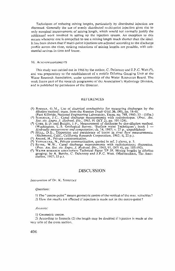
Techniques of reducing mixing lengths, particularly by distributed injection are discussed. Generally the use of evenly distributed multi-point injection gives rise to only marginal improvements of mixing length, which would not normally justify the additional work involved in setting up the injection system. An exception to this occurs whenever one is compelled to use a mixing length much shorter than the ideal. It has been shown that if multi-point injections are adjusted according to the discharge profile across the river, striking reductions of mixing lengths are possible, with sub­stantial savings in time and tracer.

10. ACKNOWLEDGEMENTS

This study was carried out in 1966 by the author, C. Delannoy and J. P. C. Watt (8), and was preparatory to the establishment of a mobile Dilution Gauging Unit at the Water Research Association, under sponsorship of the Water Resources Board. The work forms part of the research programme of the Association's Hydrology Division, and is published by permission of the Director.

REFERENCES

(1) RIMMAR, G.M., Use of electrical conductivity for measuring discharges by the dilution method ; trans, from the Russian Trudy GGI, 36, (90), pp. 18-48. (East Kilbride, National Engineering Laboratory, Trans, no. 749, 1960; 33 + (10)p.)

(2) SCHUSTER, J. C., Canal discharge measurements with radioisotopes. (Proc. Am. Soc. civ. Engrs, J. Hydraul. Div., 1965, 91 (HY 2), pp. 101-124).

(3) COBB, E .D. and BAILEY, J .F. , Measurement of discharge by dye-dilution method. (Washington, U.S. Geological Survey, 'Surface water Techniques'; book 1 — Hydraulic measurement and computation; ch. 14, 1965; v. 27 p., unpublished)

(4) HULL, D.E., Dispersion and persistence of tracer in river flow measurements. (Richmond, Calif., California Research Corporation, 1962; ii, 22 p.).

(5) ANDRÉ, H., Private communication. (6) YOTSUKURA, N., Private communication, quoted in ref. 3 above, p. 3. (') SAYRE, W.W., Canal discharge measurements with radioisotopes; discussion.

(Proc. Am. Soc. ch. Engrs, J. Hydraul. Div., 1965, 91, (HY 6), pp. 185-192). (8) WATER RESEARCH ASSOCIATION Technical Paper TP 58. Mixing lengths in dilution

gauging; by A. Barsby, C. Delannoy and J .P.C. Watt. (Medmenham, The Asso­ciation, 1967; 33 p.).

DISCUSSION

Intervention of Dr. K. SZESZTAY

Questions:

1) The "centre-point" means geometric centre of the vertical of the max. velocities ? 2) How the results are affected if injection is made not in the centre-point ?

Answers:

1) Geometric centre. 2) According to formula (2) the length may be doubled if injection is made at the

very side of the cross section.

406

Questions on Hydrometry Paper "Mixing Lengths in Dilution Gauging". A. Barsby.

1. W.G. WANNELL, Rhodesia:

Question: Has the author conducted any work on examining the reliability of Yotsukura's formulae fori ,y andN.

Reply: Unfortunately, as stated in the paper, Yotsukura does not give a guide as to how to select an appropriate value of /3 for any given case, and so it was difficult to assess the formula for Ly. Also it has been difficult in the U.K. to obtain permission to inject dyes into rivers, to enable N, the distance to the point where the tracer reaches the banks, to be determined. However, the relationship Ly = 9.N derived from equa­tions (6) and (7) certainly merits investigation as a simple and rapid means of estimating mixing lengths.

Additional reply : In a subsequent correspondence with Dr. Yotsukura, the author has learnt that (3 is indentified with the lateral dispersion coefficient.

2. Dr. K. SZESZTAY, Hungary:

Question: When single-point injection is used how is the mixing length affected by the position of the injection point across the river?

Reply: All the single-point injection tests described in this paper were carried out by injecting at the centre-line of the river, this also being the position of maximum flow in most cases. Hull's formula, equation (2), gives mixing length proportional to a constant a, equal to 50 for centre-point injection and to 200 for bank-side injection, so that bank-side injection would be expected to require four times the usual mixing length. However, in cases where the lateral velocity profile is non-uniform this factor may be expected to be much higher than four.

407