Embed Size (px)
Citation preview

University of Kentucky University of Kentucky
UKnowledge UKnowledge
Theses and Dissertations--Physics and Astronomy Physics and Astronomy
2017
Determination of Stellar Parameters through the Use of All Determination of Stellar Parameters through the Use of All
Available Flux Data and Model Spectral Energy Distributions Available Flux Data and Model Spectral Energy Distributions
Gemunu Ekanayake University of Kentucky, [email protected] Digital Object Identifier: https://doi.org/10.13023/ETD.2017.170
Right click to open a feedback form in a new tab to let us know how this document benefits you. Right click to open a feedback form in a new tab to let us know how this document benefits you.
Recommended Citation Recommended Citation Ekanayake, Gemunu, "Determination of Stellar Parameters through the Use of All Available Flux Data and Model Spectral Energy Distributions" (2017). Theses and Dissertations--Physics and Astronomy. 44. https://uknowledge.uky.edu/physastron_etds/44
This Doctoral Dissertation is brought to you for free and open access by the Physics and Astronomy at UKnowledge. It has been accepted for inclusion in Theses and Dissertations--Physics and Astronomy by an authorized administrator of UKnowledge. For more information, please contact [email protected].

STUDENT AGREEMENT: STUDENT AGREEMENT:
I represent that my thesis or dissertation and abstract are my original work. Proper attribution
has been given to all outside sources. I understand that I am solely responsible for obtaining
any needed copyright permissions. I have obtained needed written permission statement(s)
from the owner(s) of each third-party copyrighted matter to be included in my work, allowing
electronic distribution (if such use is not permitted by the fair use doctrine) which will be
submitted to UKnowledge as Additional File.
I hereby grant to The University of Kentucky and its agents the irrevocable, non-exclusive, and
royalty-free license to archive and make accessible my work in whole or in part in all forms of
media, now or hereafter known. I agree that the document mentioned above may be made
available immediately for worldwide access unless an embargo applies.
I retain all other ownership rights to the copyright of my work. I also retain the right to use in
future works (such as articles or books) all or part of my work. I understand that I am free to
register the copyright to my work.
REVIEW, APPROVAL AND ACCEPTANCE REVIEW, APPROVAL AND ACCEPTANCE
The document mentioned above has been reviewed and accepted by the student’s advisor, on
behalf of the advisory committee, and by the Director of Graduate Studies (DGS), on behalf of
the program; we verify that this is the final, approved version of the student’s thesis including all
changes required by the advisory committee. The undersigned agree to abide by the statements
above.
Gemunu Ekanayake, Student
Dr. Ronald Wilhelm, Major Professor
Dr. Christopher Crawford, Director of Graduate Studies

Determination of Stellar Parameters through the use of All Available Flux Data and
Model Spectral Energy Distributions
DISSERTATION
A dissertation submitted in partial
fulfillment of the requirements for
the degree of Doctor of Philosophy
in the College of Arts and Sciences
at the University of Kentucky
By
Gemunu Ekanayake
Lexington, Kentucky
Director: Dr. Ronald Wilhelm, Professor of Physics and Astronomy
Lexington, Kentucky 2017
Copyright c� Gemunu Ekanayake 2017

ABSTRACT OF DISSERTATION
Determination of Stellar Parameters through the use of All Available Flux Data and
Model Spectral Energy Distributions
Basic stellar atmospheric parameters, such as e↵ective temperature, surface gravity,
and metallicity plays a vital role in the characterization of various stellar popula-
tions in the Milky Way. The Stellar parameters can be measured by adopting one
or more observational techniques, such as spectroscopy, photometry, interferometry,
etc. Finding new and innovative ways to combine these observational data to de-
rive reliable stellar parameters and to use them to characterize some of the stellar
populations in our galaxy is the main goal of this thesis.
Our initial work, based on the spectroscopic and photometric data available in
literature, had the objective of calibrating the stellar parameters from a range of
available flux observations from far-UV to far-IR. Much e↵ort has been made to
estimate probability distributions of the stellar parameters using Bayesian inference,
rather than point estimates.
We applied these techniques to blue straggler stars (BSSs) in the galactic field,
which are thought to be a product of mass transfer mechanism associated with binary
stars. Using photometry available in SDSS and GALEX surveys we identified 85
stars with UV excess in their spectral energy distribution (SED) : indication of a
hot white dwarf companion to BSS. To determine the parameter distributions (mass,

temperature and age) of the WD companions, we developed algorithms that could
fit binary model atmospheres to the observed SED. The WD mass distribution peaks
at 0.4M�, suggests the primary formation channel of field BSSs is Case-B mass
transfer, i.e. when the donor star is in red giant phase of its evolution. Based
on stellar evolutionary models, we estimate the lower limit of binary mass transfer
e�ciency � ⇠ 0.5.
Next, we have focused on the Canis Major overdensity (CMO), a substructure
located at low galactic latitude in the Milky Way, where the interstellar reddening
(E(B�V )) due to dust is significantly high. In this study we estimated the reddening,
metallicity distribution and kinematics of the CMO using a sample of red clump (RC)
stars. The average E(B�V ) (⇠ 0.19) is consistent with that measured from Schlegel
maps (Schlegal et.al. 1998). The overall metallicity and kinematic distribution is
in agreement with the previous estimates of the disk stars. But the measured mean
alpha element abundance is relatively larger with respect to the expected value for
disk stars.
KEYWORDS: Stellar parameters, Kurucz models, Blue straggler, Canis Major Over-
density, Red clump
Gemunu Ekanayake
May 4, 2017

Determination of Stellar Parameters through the use of All Available Flux Data and
Model Spectral Energy Distributions
By
Gemunu Ekanayake
Director of Dissertation: Ronald Wilhelm
Director of Graduate Studies: Christopher Crawford
Date: May 4, 2017

ACKNOWLEDGMENTS
I would like to thank my advisor Prof. Ronald Wilhelm for all the support and
guidance given throughout all these years. I’m eternally grateful for the opportunity
you gave me to conduct research in astronomy. Most importantly thank you for being
an awesome human being.
I also thank my committee members Prof. Renbin Yan, Prof. Thomas Troland
and Prof. Sebasthiyan Bryson for their diverse guidance.
Last but not least, I would like to thank my parents and my sisters for their
unconditional support.
iii
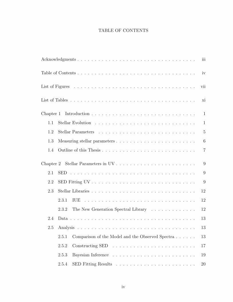
TABLE OF CONTENTS
Acknowledgments . . . . . . . . . . . . . . . . . . . . . . . . . . . . . . . . . . iii
Table of Contents . . . . . . . . . . . . . . . . . . . . . . . . . . . . . . . . . . iv
List of Figures . . . . . . . . . . . . . . . . . . . . . . . . . . . . . . . . . . . vii
List of Tables . . . . . . . . . . . . . . . . . . . . . . . . . . . . . . . . . . . . xi
Chapter 1 Introduction . . . . . . . . . . . . . . . . . . . . . . . . . . . . . . 1
1.1 Stellar Evolution . . . . . . . . . . . . . . . . . . . . . . . . . . . . . 1
1.2 Stellar Parameters . . . . . . . . . . . . . . . . . . . . . . . . . . . . 5
1.3 Measuring stellar parameters . . . . . . . . . . . . . . . . . . . . . . . 6
1.4 Outline of this Thesis . . . . . . . . . . . . . . . . . . . . . . . . . . . 7
Chapter 2 Stellar Parameters in UV . . . . . . . . . . . . . . . . . . . . . . . 9
2.1 SED . . . . . . . . . . . . . . . . . . . . . . . . . . . . . . . . . . . . 9
2.2 SED Fitting UV . . . . . . . . . . . . . . . . . . . . . . . . . . . . . . 9
2.3 Stellar Libraries . . . . . . . . . . . . . . . . . . . . . . . . . . . . . . 12
2.3.1 IUE . . . . . . . . . . . . . . . . . . . . . . . . . . . . . . . . 12
2.3.2 The New Generation Spectral Library . . . . . . . . . . . . . 12
2.4 Data . . . . . . . . . . . . . . . . . . . . . . . . . . . . . . . . . . . . 13
2.5 Analysis . . . . . . . . . . . . . . . . . . . . . . . . . . . . . . . . . . 13
2.5.1 Comparison of the Model and the Observed Spectra . . . . . . 13
2.5.2 Constructing SED . . . . . . . . . . . . . . . . . . . . . . . . 17
2.5.3 Bayesian Inference . . . . . . . . . . . . . . . . . . . . . . . . 19
2.5.4 SED Fitting Results . . . . . . . . . . . . . . . . . . . . . . . 20
iv

2.6 Summary . . . . . . . . . . . . . . . . . . . . . . . . . . . . . . . . . 22
Chapter 3 Blue Straggler Stars in the Galactic Field . . . . . . . . . . . . . . 24
3.1 Introduction . . . . . . . . . . . . . . . . . . . . . . . . . . . . . . . . 24
3.1.1 Blue Straggler Stars . . . . . . . . . . . . . . . . . . . . . . . 24
3.1.2 Mass Transfer via Roche-Lobe Overflow . . . . . . . . . . . . 26
3.1.3 Field Blue Straggler Stars . . . . . . . . . . . . . . . . . . . . 28
3.1.4 White Dwarf Stars . . . . . . . . . . . . . . . . . . . . . . . . 29
3.2 Analysis . . . . . . . . . . . . . . . . . . . . . . . . . . . . . . . . . . 30
3.2.1 Identification of Field Blue Straggler Stars . . . . . . . . . . . 30
3.2.2 SDSS Data . . . . . . . . . . . . . . . . . . . . . . . . . . . . 30
3.2.3 GALEX Data . . . . . . . . . . . . . . . . . . . . . . . . . . . 32
3.2.4 Cross-Identification of sources . . . . . . . . . . . . . . . . . . 34
3.2.5 Extinction Correction . . . . . . . . . . . . . . . . . . . . . . . 35
3.2.6 UV-Excess Stars . . . . . . . . . . . . . . . . . . . . . . . . . 36
3.2.7 Temperature Sanity Check . . . . . . . . . . . . . . . . . . . . 37
3.2.8 BSS-WD Fitting . . . . . . . . . . . . . . . . . . . . . . . . . 41
3.2.9 Synthetic Fluxes . . . . . . . . . . . . . . . . . . . . . . . . . 43
3.2.10 Observed Fluxes . . . . . . . . . . . . . . . . . . . . . . . . . 43
3.2.11 SED Fitting . . . . . . . . . . . . . . . . . . . . . . . . . . . . 44
3.2.12 Distribution of WD parameters . . . . . . . . . . . . . . . . . 46
3.2.13 Mass Transfer e�ciency . . . . . . . . . . . . . . . . . . . . . 50
3.3 Summary . . . . . . . . . . . . . . . . . . . . . . . . . . . . . . . . . 54
Chapter 4 Canis Major Overdensity . . . . . . . . . . . . . . . . . . . . . . . 56
4.1 Introduction . . . . . . . . . . . . . . . . . . . . . . . . . . . . . . . . 56
4.1.1 Red Clump Stars . . . . . . . . . . . . . . . . . . . . . . . . . 57
4.1.2 Observational Data . . . . . . . . . . . . . . . . . . . . . . . . 59
v
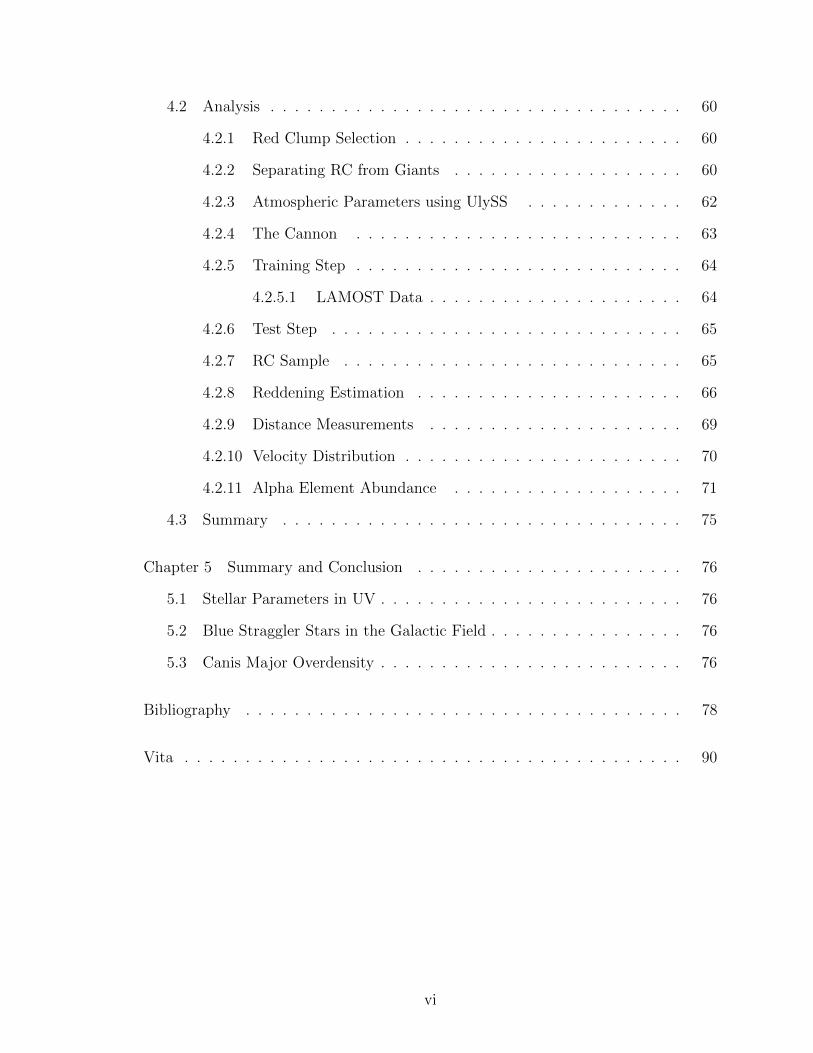
4.2 Analysis . . . . . . . . . . . . . . . . . . . . . . . . . . . . . . . . . . 60
4.2.1 Red Clump Selection . . . . . . . . . . . . . . . . . . . . . . . 60
4.2.2 Separating RC from Giants . . . . . . . . . . . . . . . . . . . 60
4.2.3 Atmospheric Parameters using UlySS . . . . . . . . . . . . . 62
4.2.4 The Cannon . . . . . . . . . . . . . . . . . . . . . . . . . . . 63
4.2.5 Training Step . . . . . . . . . . . . . . . . . . . . . . . . . . . 64
4.2.5.1 LAMOST Data . . . . . . . . . . . . . . . . . . . . . 64
4.2.6 Test Step . . . . . . . . . . . . . . . . . . . . . . . . . . . . . 65
4.2.7 RC Sample . . . . . . . . . . . . . . . . . . . . . . . . . . . . 65
4.2.8 Reddening Estimation . . . . . . . . . . . . . . . . . . . . . . 66
4.2.9 Distance Measurements . . . . . . . . . . . . . . . . . . . . . 69
4.2.10 Velocity Distribution . . . . . . . . . . . . . . . . . . . . . . . 70
4.2.11 Alpha Element Abundance . . . . . . . . . . . . . . . . . . . 71
4.3 Summary . . . . . . . . . . . . . . . . . . . . . . . . . . . . . . . . . 75
Chapter 5 Summary and Conclusion . . . . . . . . . . . . . . . . . . . . . . 76
5.1 Stellar Parameters in UV . . . . . . . . . . . . . . . . . . . . . . . . . 76
5.2 Blue Straggler Stars in the Galactic Field . . . . . . . . . . . . . . . . 76
5.3 Canis Major Overdensity . . . . . . . . . . . . . . . . . . . . . . . . . 76
Bibliography . . . . . . . . . . . . . . . . . . . . . . . . . . . . . . . . . . . . 78
Vita . . . . . . . . . . . . . . . . . . . . . . . . . . . . . . . . . . . . . . . . . 90
vi

LIST OF FIGURES
1.1 Hertzsprung-Russel diagram for globular cluster M55. Adopted from
http://www.atnf.csiro.au/outreach/education/senior/astrophysics/
stellarevolution_clusters.html . . . . . . . . . . . . . . . . . . . . . 3
2.1 The sensitivity of flux distributions to Te↵, log g and [M/H]. The solid line
is for a model with Te↵ = 7500, log g = 4.0 and [M/H] = 0.0. The dotted
and dashed lines indicate models with one of the parameters adjusted, as
indicated. All fluxes have been normalized to zero at 5556. . . . . . . . . 10
2.2 Comparison of the observed spectrum with the best fitting model spectrum
for stars in our study. . . . . . . . . . . . . . . . . . . . . . . . . . . . . . 15
2.3 Comparison of the observed spectrum with the best fitting model spectrum
for stars in our study. . . . . . . . . . . . . . . . . . . . . . . . . . . . . . 16
2.4 Passband response functions from which synthetic magnitudes have been
computed. All curves are normalized to one, and as shown as function of
wavelength. . . . . . . . . . . . . . . . . . . . . . . . . . . . . . . . . . . 18
2.5 Example posterior joint distribution between Teff and log g for a star in
our study. Color bar on right of plot represent the probability. . . . . . . 21
3.1 Observed CMD for M67. The axes are the color and magnitude la-
beled with the central wavelengths. The pentagonal points are the blue
stragglers more luminous than the main-sequence turno↵, the squares
the intermediate-color stragglers and clump giants, including one possi-
ble AGB star.Adopted from [27] . . . . . . . . . . . . . . . . . . . . . . . 25
vii

3.2 The evolutionary pathway to produce blue straggler stars (BSSs) through
mass transfer. First the bigger primary evolves o↵ the main sequence
and fills its Roche lobe. Then secondary gains mass from the primary
becoming a BSS . . . . . . . . . . . . . . . . . . . . . . . . . . . . . . . . 27
3.3 The color selection in u-g and g-r used to select BHB and BS stars.
Adopted from Xue et.al. [36] . . . . . . . . . . . . . . . . . . . . . . . . 32
3.4 BSS-BHB separation in SDSS data using the stellar parameters . . . . . 33
3.5 Transmission curves for GALEX bandpasses . . . . . . . . . . . . . . . . 34
3.6 Footprints of the SDSS (green), GALEX AIS (blue) and MIS (red) imaging
surveys [38] . . . . . . . . . . . . . . . . . . . . . . . . . . . . . . . . . . 35
3.7 Stellar parameter distributions for filed BSSs selected in this study . . . 36
3.8 (FUV-NUV) vs. SDSS/DR7 Te↵ values from GALEX-SDSS data. Sym-
bols denote 1 kK bins in Te↵. Solid symbols denote the stars used to define
the upper (FUV-NUV) - Te↵ diagonal sequence and calibrate this color
from their Te↵ values. The dot-dashed locus separates the calibration
sequence from the UV-excess population in the lower left. [43] . . . . . . 38
3.9 Comparison of temperatures of BSSs in this work with SSPP . . . . . . . 40
3.10 (FUV-NUV) vs. SSPP temperature values from SDSS-GALEX data. The
red dashed line is the 2� deviation from the fit to the diagonal sequence.
Stars located left to this line are BSS with UV-excess. . . . . . . . . . . . 41
3.11 Example of BSS+WD fitting. Orange circles are the observed FUV,NUV
and u photometry. Blue and Red lines represent the synthetic spectra
of BS (ATLAS9- Kurucz) and WD (Bergeron) respectively.Grey is the
combined best fit spectrum for observed photometry. . . . . . . . . . . . 47
3.12 White Dwarf parameters . . . . . . . . . . . . . . . . . . . . . . . . . . . 48
viii

3.13 This figure adopted from [52] shows the comparison of the SDSS DR7 WD
mass distributions from their work (black) and Kleinman et al. (2013,
filled blue). The low-mass objects (red; M < 0.45 M�) are thought to be
the WD originated from binary mass transfer processes. . . . . . . . . . . 50
3.14 Theoretical mass-age relations from BaSTI evolutionary models. . . . . . 53
3.15 Cumulative distribution of mass transfer e�ciency . . . . . . . . . . . . . 54
4.1 Latitude profiles of a 2MASS M-giant star sample selected around CMa.
Upper-left panel assumes a North/South symmetry around b = 0� , lower-
left panel assumes a warp amplitude of 2� in the southern direction. Star
counts in left panels are corrected for reddening using the Schlegel et al.
maps. Right panels show the same plots, except for correcting the Schlegel
et al. values with the formula given in Bonifacio et al. showing the CMa
over-density has almost disappeared. . . . . . . . . . . . . . . . . . . . . 58
4.2 The number of red clump stars in the solar neighborhood, based on Hip-
parchus data,is shown as a function of absolute magnitude of I band with
the thin solid line (fit and histogram).The number of red clump stars in
the G302 field (Holland et al. 1996), is shown as a function of absolute
magnitude with thick solid line. All distributions are normalized. Adopted
from [66] . . . . . . . . . . . . . . . . . . . . . . . . . . . . . . . . . . . . 59
4.3 The CMD in the V vs V-I plane of all stars in the direction of the CMO.
Data points in red indicate stars belonging to the red clump. For the
clarity the Blue Plume stars are also highlighted in blue. . . . . . . . . . 61
4.4 The stellar parameters derived from ULySS spectrum fitting. . . . . . . . 63
4.5 First-order coe�cients and scatter of the spectral model. . . . . . . . . . 66
4.6 Stellar parameters derived from The Cannon. . . . . . . . . . . . . . . . 67
4.7 Stellar parameters derived from The Cannon. . . . . . . . . . . . . . . . 68
4.8 Heliocentric distance distribution of RC stars. . . . . . . . . . . . . . . . 70
ix
4.9 BSS-BHB separation in SDSS data using the stellar parameters . . . . . 72
4.10 Stellar distribution of stars in the [/Fe] vs. [Fe/H] plane as a function of
R and |z|. . . . . . . . . . . . . . . . . . . . . . . . . . . . . . . . . . . 73
4.11 Distribution of stars in the [/Fe] vs. [Fe/H] plane for our stars. . . . . . . 73
4.12 Distribution of the height to the stars from the Galactic plane. . . . . . 74
x

LIST OF TABLES
2.1 Stellar parameters obtained from SED fitting compares to published values
(column format is published/SED fitting) . . . . . . . . . . . . . . . . . 22
3.1 Extinction in di↵erent passbands . . . . . . . . . . . . . . . . . . . . . . 37
3.2 Stellar parameters and photometry of UV-excess BSS . . . . . . . . . . . 42
3.3 Bolometric Corrections by Flower (1996) as a Function of Temperature:
BCv = a+ b(logTeff ) + c(logTeff )2 + ... . . . . . . . . . . . . . . . . . . 46
3.4 Stellar Parameters of WD stars . . . . . . . . . . . . . . . . . . . . . . . 51
xi

Chapter 1 Introduction
The universe as we find it today, was created by the Big Bang about 13.8 Gyrs ago
([1]). After few billion years after the Big Bang, the Galaxies are formed. Understand-
ing how these Galaxies formed and evolved through time is one of the fundamental
objectives in modern astronomy.
Our home in the universe, Milky Way, gives us an unique opportunity to achieve
this goal by measuring and analyzing the stars spread throughout the Galaxy. The
Milky way galaxy consists of several billion stars of di↵erent ages, masses and sizes.
The determination exact distribution of these stars is a di�cult task, simply because
we are living inside of it. But thanks to modern astronomy we have a good enough
picture about the structure of our Galaxy. Milky way consists various stellar popu-
lations, each characterized by distinct spatial distribution, kinematics, and chemical
content. The Milky Way is usually modeled by three discrete components;the thin
disk, the thick disk, and the halo. However, these are by no means pure smooth dis-
tributions of stars, but rather combination of many di↵erent substructures. Due to
the invention of modern sky surveys, evidence for much more complex substructures
like stellar streams and overdensities are found.
Stars with initial masses between about 0.8 and 8 M� dominate the stellar pop-
ulations in our Milky Way Galaxy. In this thesis we will be concerned with such
low-intermediate mass stars, therefore the following discussion on stellar evolution is
limited only to those stars.
1.1 Stellar Evolution
After the big-bang only hydrogen, helium and traces of lithium and deuterium were
formed. All other elements identified today, including the main component of human
1

bodies, carbon, were formed later. Most elements lighter than iron are formed in
main-sequence and old stars, while elements heavier than iron are originated in dying
stars. Stars consist of roughly 6% percent of the baryonic matter [2].
According to recent observational studies, long thin filaments were formed inside
molecular clouds and, next, these filaments fragment into protostellar cores due to
gravitational instability, when their linear density exceeds a certain threshold. [3] An
object may be called a star if it is able to generate energy by nuclear fusion at a level
su�cient to stop the contraction due to gravity.
A star like the sun, but in general all the low-intermediate stars with masses
between 1-8 M� spend almost 90% of their life on the main sequence (MS) of the
Hertzsprung-Russel diagram, which represents the luminosity of a star as a function
of its e↵ective temperature (Figure 1.1).
At this stage, stars keep their equilibrium through thermonuclear reactions, p-p
chain or the CNO cycle, which convert Hydrogen into Helium. When a star exhausts
its initial hydrogen supply in the core, the main sequence phase arrives to its end
and the star begins to contract until the temperature and density are high enough to
ignite hydrogen in a shell around the hydrogen-exhausted core. This, in turn, causes
the star to expand and climb up the Red Giant Branch (RGB)
The evolution on the red giant branch is much faster than main sequence phase.
When hydrogen exhausted in the core, the star begins to burn hydrogen in a shell
around the core. when the convection in the envelope moves in to the region where
nuclear reactions taking place, it can dredges up the material that has been produced
by p-p chain and CNO cycle. This could alter the chemical composition of the outer
surface of the star. At this stage the star starts to loose mass from its outer boundary
through a slow stellar wind.
Stars with initial mass less than 2.2 M� develop a semi-degenerate core during
the RGB phase. It accretes mass from the shell without contracting and remains
2
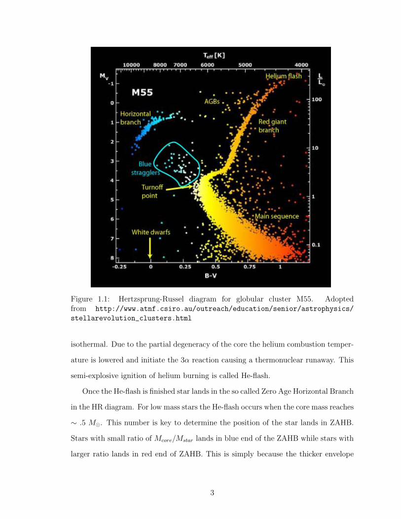
Figure 1.1: Hertzsprung-Russel diagram for globular cluster M55. Adoptedfrom http://www.atnf.csiro.au/outreach/education/senior/astrophysics/
stellarevolution_clusters.html
isothermal. Due to the partial degeneracy of the core the helium combustion temper-
ature is lowered and initiate the 3↵ reaction causing a thermonuclear runaway. This
semi-explosive ignition of helium burning is called He-flash.
Once the He-flash is finished star lands in the so called Zero Age Horizontal Branch
in the HR diagram. For low mass stars the He-flash occurs when the core mass reaches
⇠ .5 M�. This number is key to determine the position of the star lands in ZAHB.
Stars with small ratio of Mcore/Mstar lands in blue end of the ZAHB while stars with
larger ratio lands in red end of ZAHB. This is simply because the thicker envelope
3
able to shield the hotter star and appear redder and cooler. For these reasons stars
with intermediate mass occupy the reddest part of the ZAHB, creating the so called
red-clump. During horizontal branch phase stars burn helium in their cores stably,
via 3↵ reaction. Once the helium is exhausted in the core star starts to move towards
the Asymptotic Giant Branch (AGB).
At the end of HB phase, stellar core consisting of carbon and oxygen. During
the early AGB (EAGB) phase the shell of hydrogen, still on, continues to deposit
helium in the layer that separates it from the core of C-O, making it more and more
degenerate. Again similar to He-flash, the degeneracy lowers the ignition temperature
of the helium until the shell lights up in a semi-explosive way. The shell of helium
becomes dominant, and continues to deposit CO on the core, making it more and
more degenerate. At the same time the inter-shell stops progressively to expand until
the shell of hydrogen returns to dominate. During this phase of EAGB, the stars
with the mass larger than 4.6M�
can experience the second chemical mixing process. As already mentioned, the
expansion of the structure allow the convection layers to penetrate from the outside.
If this is su�ciently deep to arrive to the inter-shell, it can bring the elements such
as He, C, N, O, to the surface which are the products of combustion of hydrogen.
The next phase is called Thermally Pulsing AGB (TPAGB) and during this period
stars experience multiple thermal pulses. The fundamental process that occurs during
TPAGB is the third dredge-up. The mixing during third dredge-up involves extremely
profound regions of the star (⇠ 75 percent of the structure) and generates chemical
signatures that di↵er form those characterizing the other two dredge-ups, such as an
increase of the abundance of carbon at the surface.
During the entire duration of the AGB phase, the stars su↵er substantial mass
loss. This is due to the fact that the envelope of these stars is expanded and cooled,
therefore causing to from layers of molecules and dust, which are then removed as
4

stellar wind by the e↵ect of radiation pressure.
After about a dozen thermal pulses, the latest expansion is su�cient to allow the
release of the outermost layers around the nucleus of CO which is rapidly becoming
fully degenerate. With this phase, known as post-AGB, the nuclear-active evolution
of the stars ends leading to the final stages of a stars life.
Stars with low-intermediate mass end their life cycle as white dwarf stars. The
white dwarfs consists of the fully degenerate core and very thin outer layer. These
objects evolve by cooling down at constant radius.
1.2 Stellar Parameters
In order to fully describe a star, a number of parameters should be known. The
mass M, the luminosity L, and the radius R can be considered as the first order
parameters that describe a star. Models of stellar evolution and stellar atmospheres
are based on these parameters. In order to test stellar evolution theory and the
stellar atmosphere theory, high-precision measured fundamental parameters for stars
in various evolutionary stages are needed.
The set of parameters based on L,M and R are used in studies that are closer
to directly observed quantities. Among those the e↵ective temperature Teff and the
logarithmic of surface gravity log g are the most useful parameters, given by following
equations.
Teff =L
4⇡R2�(1.1)
where, � is the Stefan-Boltzmann constant.
g =GM
R2(1.2)
where G is the gravitational constant.
5
Most evolutionary calculations are presented as isochrones, i.e. mass dependent
tracks of constant age, in a HR diagram.
In addition to the e↵ective temperature and the surface gravity, the chemical
composition of a star is required to fully understand the system.
Most common term used in astronomy to describe the chemical composition of an
astronomical object is called metallicity (Z), which is the mass fraction of elements
which have larger atomic numbers that hydrogen or helium. Together with the mass
fraction of hydrogen (X) and helium (Y ) that covers the whole range of elements
(with Z +X +Y = 1). One often use the solar metallicity Z = 0.0169 as a reference,
with X = 0.7346 and Y = 0.2485 ([4]). The metallicity is an important attribute
since it will e↵ect the properties of a galaxy. Typically only one mettalicty is being
measured. For example the Fe abundance, since it is usually the easiest to measure.
The usual convention is to represent the metallicity with respect to the value of the
sun. i.e
[Fe/H] = log10(Fe/H)
(Fe/H)�(1.3)
In addition to the parameters discussed above, few more parameters may be re-
quired to fully describe the physics of a star. These parameters include angular
momentum, magnetic field, mass loss rate and pulsation period.
All of these parameters evolve as a function of time, where the zero-point is usually
defined when the star appears first on the main sequence, i.e. the so so-called zero age
main sequence (ZAMS). Therefore in order to compare the observations to theoretical
models, the age of the star is required as an additional parameter in some cases.
1.3 Measuring stellar parameters
Fundamental stellar parameters mentioned in previous section, such as e↵ective tem-
perature and surface gravity, can be measured using one (or more) of several types
6
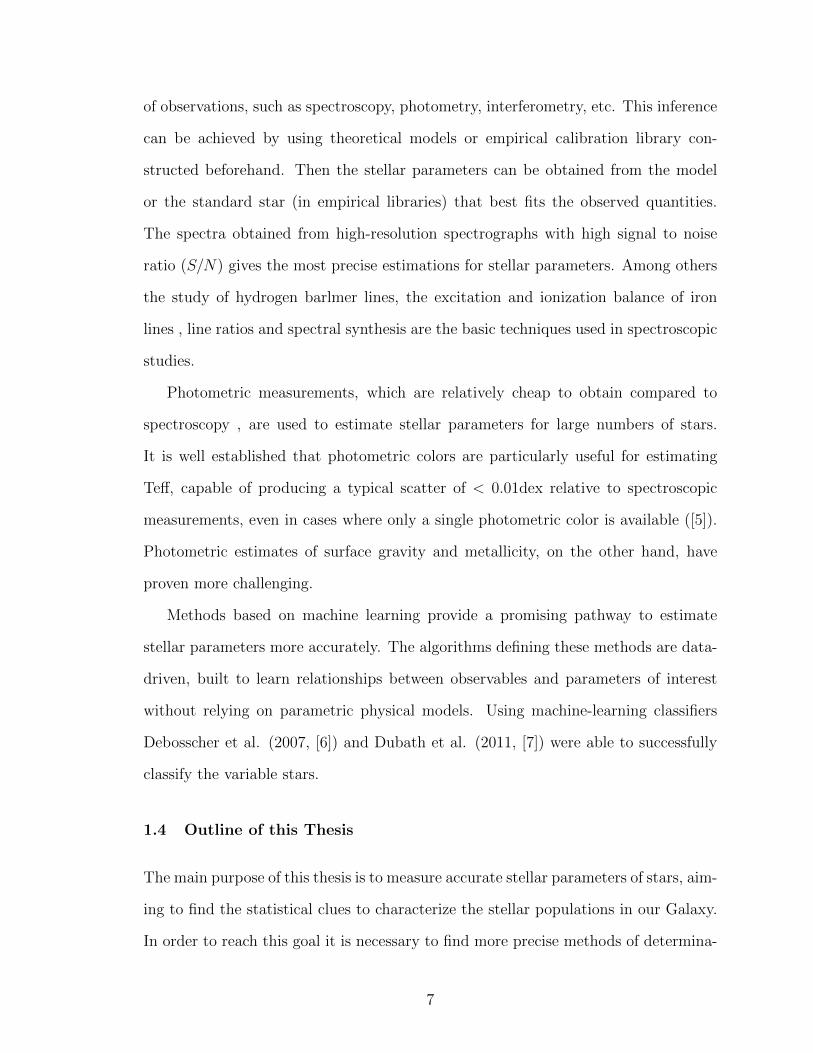
of observations, such as spectroscopy, photometry, interferometry, etc. This inference
can be achieved by using theoretical models or empirical calibration library con-
structed beforehand. Then the stellar parameters can be obtained from the model
or the standard star (in empirical libraries) that best fits the observed quantities.
The spectra obtained from high-resolution spectrographs with high signal to noise
ratio (S/N) gives the most precise estimations for stellar parameters. Among others
the study of hydrogen barlmer lines, the excitation and ionization balance of iron
lines , line ratios and spectral synthesis are the basic techniques used in spectroscopic
studies.
Photometric measurements, which are relatively cheap to obtain compared to
spectroscopy , are used to estimate stellar parameters for large numbers of stars.
It is well established that photometric colors are particularly useful for estimating
Te↵, capable of producing a typical scatter of < 0.01dex relative to spectroscopic
measurements, even in cases where only a single photometric color is available ([5]).
Photometric estimates of surface gravity and metallicity, on the other hand, have
proven more challenging.
Methods based on machine learning provide a promising pathway to estimate
stellar parameters more accurately. The algorithms defining these methods are data-
driven, built to learn relationships between observables and parameters of interest
without relying on parametric physical models. Using machine-learning classifiers
Debosscher et al. (2007, [6]) and Dubath et al. (2011, [7]) were able to successfully
classify the variable stars.
1.4 Outline of this Thesis
The main purpose of this thesis is to measure accurate stellar parameters of stars, aim-
ing to find the statistical clues to characterize the stellar populations in our Galaxy.
In order to reach this goal it is necessary to find more precise methods of determina-
7

tion of stellar parameters, especially the e↵ective temperature (Teff ), surface gravity
(log g) and metallicity ([Fe/H]). To achieve this, several techniques were imple-
mented such that all available data being used to construct the energy distribution
of a given star.
At first we studied the Spectral Energy Distributions (SED) of old metal poor
A-type stars aiming to upgrade the UV calibration of these stars. For that we used
a sample of stars that have IUE and NGSL spectra in addition to the accurate pho-
tometry. Here we introduced a probabilistic method to infer stellar parameters using
the observed SED. This study is presented in Chapter 2.
In Chapter 3 we present the results of detecting the Blue Straggler-White Dwarf
(BSS-WD) binaries in the Galactic field. The fitting using the composite SED of the
binary we identified eighty stars with WD companions. Here we present the potential
mass transfer histories based on the parameters determined via SED fitting.
In chapter 4 we present a study on Canis Major Overdensity (CMO). We used
data-driven method to infer the stellar parameters of the sample of stars towards CMO
in order to select Red Clump (RC) stars. We used RC to measure the reddening,
kinematics and chemical content towards the CMO.
8

Chapter 2 Stellar Parameters in UV
2.1 SED
The observed spectral energy distribution (SED) of a star can reveal a lot information
about the properties of the star. The total radiation emitted by a star depends on
various complex physical processes of the star and one has to be able to disentangle the
components which make up the SED in order to understand those physical processes.
The radiation received at the Earth surface depends not only on the radiation emitted
by the star alone, but also on the interstellar processes that modifies the SED by
absorbtion and scattering of the photons.
Stellar SED can be studied by using broad band photometry, where the flux is
measured over a certain range of wavelength. The flux in di↵erent bands is measured
via a filter which will only let through light of certain wavelengths, in a range specific
for each band. Depending on the specifications of the telescope and the instrument,
the flux is only measured in a limited number of bands. Therefore, to fully sample
the SED of a star, a combination of instruments/telescopes is necessary.
To be able to determine the stellar atmospheric parameters that shaped the flux
distribution coming out of the star we need to fit the model atmosphere flux to the
observations.
2.2 SED Fitting UV
The importance of using ultra-violet photometry in stellar studies was pointed out
in many studies (eg.[8]). UV is useful in characterizing the metalicity and the star
formation history of young stellar populations ([9]), to study the ↵ element enhance-
ment of stars ([10]) and to estimate the uv-upturn ([11], [12]) or the contribution of
9

blue horizontal branch stars to the integrated flux in galaxies.
Figure 2.1: The sensitivity of flux distributions to Te↵, log g and [M/H]. The solidline is for a model with Te↵ = 7500, log g = 4.0 and [M/H] = 0.0. The dotted anddashed lines indicate models with one of the parameters adjusted, as indicated. Allfluxes have been normalized to zero at 5556.
In a simple stellar population (SSP) the blue wavelengths are highly sensitive to
the hot stars like main-sequence turno↵, blue horizontal branch(BHB) or blue strag-
10

gler stars (BSSs). Figure 2.1 shows the sensitivity of the flux distribution to the
various atmospheric parameters for an A-type model star. There is significant varia-
tion in the fluxes in UV region compare to the optical part when the model parameters
are varied. The luminosity from these stars can have an important contribution to
the integrated spectra ([13],[14]). It is vital to distinguish between the old and young
stellar populations that contribute to the UV flux in order to properly characterize
the stellar population. That process relies on identifying the di↵erent contribution to
the di↵erent parts of the spectral energy distribution (SED). Therefore, combining
optical and UV data is important aspect in SED studies. ([15])
Overwhelming majority of studies use Kurucz atmospheric models when compar-
ing observed SED to synthetic SED to determine the stellar parameters. In optical
wavelengths these synthetic spectra agreed fairly well with energy distributions of real
stars having the same physical parameters. However, when fitting with UV fluxes
the disagreement occurred between the model and observed fluxes. This is especially
noticeable in the studies done using the earlier version of Kurucz models.([16]) Later
Kurucz developed improved version of models with new opacity distribution functions
(ODFs), with new atomic and molecular lines and were successful to certain degree
in solving the issue of UV fluxes.
The object of this chapter is to determine how the UV flux of A-type stars like
blue stragglers or blue horizontal branch stars a↵ect the stellar parameter determi-
nation via SED fitting. Here we present our method of multi-band SED fitting based
on Bayesian probabilistic inference to determine the stellar atmospheric parameters
which uses all the available photometric data for a given object. We test our method
for sample of A-type stars (either BHB or BSS) that have good spectroscopic and/or
photometric data and well determined stellar parameters.
11

2.3 Stellar Libraries
In order to study the UV behavior in SEDs of blue horizontal branch and blue strag-
gler stars we require stars that have good spectroscopic data from far UV to near IR.
Unfortunately most spectral libraries limited to the optical region of the SED. The
lack of libraries extending blueward 3500 A has prevented the building of models that
allow us to perform detailed studies, such as those performed in the optical range.
2.3.1 IUE
This is the fist available stellar UV library ([17]). This contains low resolution spectra
for about 218 stars mostly with solar metallicity. The spectra were collected from
International Ultraviolet Explorer (IUE) satellite, with wavelength coverage 1300 to
3400 ([18]). The library essentially composed of stars exhibiting normal behavior in
the ultraviolet. Even though this is quite a small sample when compare to the size
of the modern optical libraries, the di↵erence between the available optical and UV
libraries is quite significant. One of the shortcomings of the IUE is that the coverage
in metallicity is mostly limited to solar values. According to our estimates only about
30 stars of the library have the metallicities less than -1.
2.3.2 The New Generation Spectral Library
A significant step regarding UV spectral libraries was later made by the New Genera-
tion Spectral Library (NGSL) (2009,[19]). The observation were made by the Imaging
Spectrograph (STIS) onboard the Hubble Space Telescope (HST). The stellar spectra
of the NGSL cover the range 2300-9000 at resolution R ⇠ 1000. But unlike the IUE,
it does not reach the Far UV wavelengths. However the 374 stars of this library were
rigorously chosen to have a good coverage in the space of atmospheric parameters.
NGSL spectra have a good coverage of stellar atmospheric parameters, with metallic-
12
ities between -2.0 dex and 0.5 dex and spectral types from O to M for all luminosity
classes.
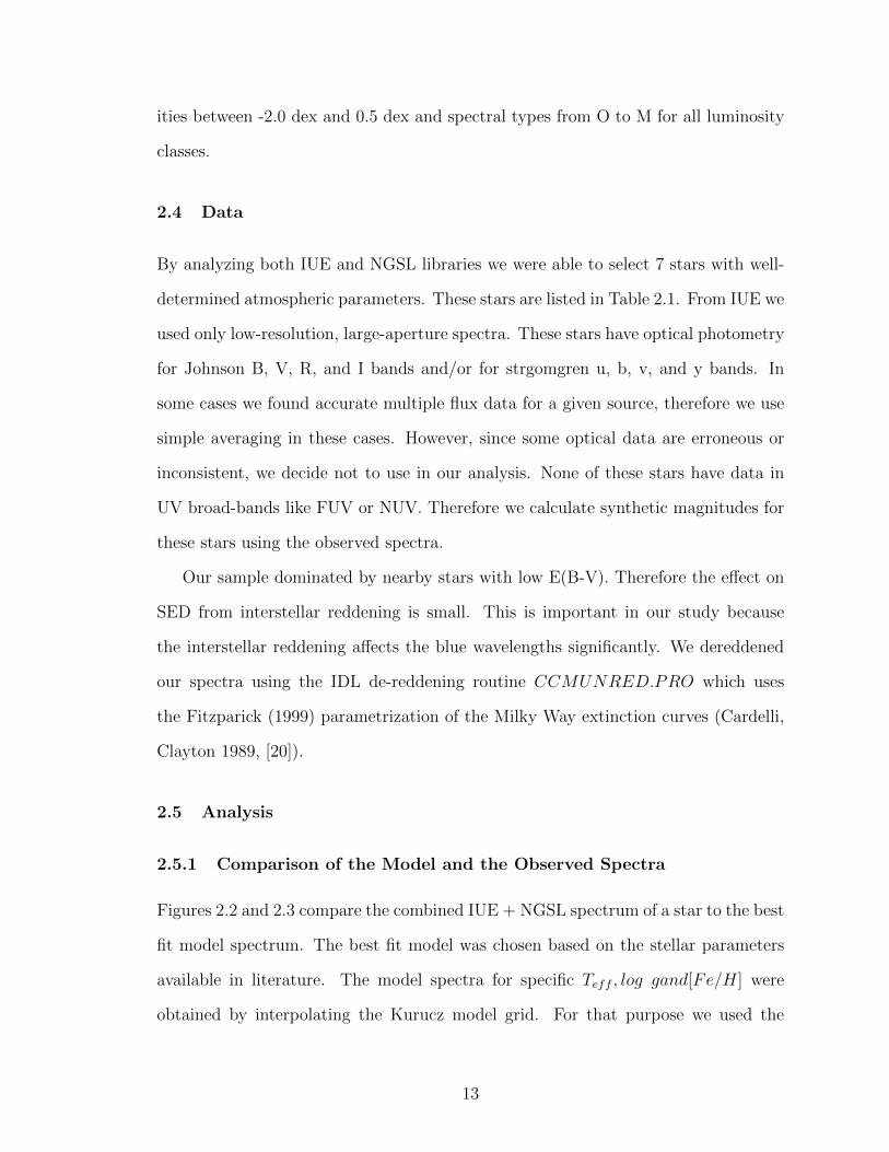
2.4 Data
By analyzing both IUE and NGSL libraries we were able to select 7 stars with well-
determined atmospheric parameters. These stars are listed in Table 2.1. From IUE we
used only low-resolution, large-aperture spectra. These stars have optical photometry
for Johnson B, V, R, and I bands and/or for strgomgren u, b, v, and y bands. In
some cases we found accurate multiple flux data for a given source, therefore we use
simple averaging in these cases. However, since some optical data are erroneous or
inconsistent, we decide not to use in our analysis. None of these stars have data in
UV broad-bands like FUV or NUV. Therefore we calculate synthetic magnitudes for
these stars using the observed spectra.
Our sample dominated by nearby stars with low E(B-V). Therefore the e↵ect on
SED from interstellar reddening is small. This is important in our study because
the interstellar reddening a↵ects the blue wavelengths significantly. We dereddened
our spectra using the IDL de-reddening routine CCMUNRED.PRO which uses
the Fitzparick (1999) parametrization of the Milky Way extinction curves (Cardelli,
Clayton 1989, [20]).
2.5 Analysis
2.5.1 Comparison of the Model and the Observed Spectra
Figures 2.2 and 2.3 compare the combined IUE + NGSL spectrum of a star to the best
fit model spectrum. The best fit model was chosen based on the stellar parameters
available in literature. The model spectra for specific Teff , log gand[Fe/H] were
obtained by interpolating the Kurucz model grid. For that purpose we used the
13

spectrum synthesis package, SPECTRUM ([21]). SPECTRUM synthesizes stellar
spectra assuming a plane-parallel atmosphere geometry and local thermal equilibrium
(LTE) which is consistent with Kurucz ATLAS12 models. we interpolate the Kurucz
models using kmod IDL package.1. kmod interpolates linearly a Kurucz model for
the desired values of e↵ective temperature, surface gravity and metallicity using 8
surrounding models.
For all the stars in our sample the matching between energy distributions is rel-
atively good. However, some stars show deviation from the model spectrum at FUV
wavelengths. For example the stars HD86986, HD2857, HD74721 and HD109995
show larger flux relative to the model spectrum below 2000 A. We estimate this
di↵erence by taking the average flux in the region below 2000 A for both spectra, and
noticed that observed spectra have 10-15 % stronger flux in far-UV. But if we take
in to account the estimated errors for these parameters this di↵erence can be easily
accounted for.
Based on this investigation we can conclude that the Kurucz ATLAS12 models
agree quite well with the observed energy distributions of low-matallicity BHB or
BSS stars.
1http://www.as.utexas.edu/ hebe/
14

Figure 2.2: Comparison of the observed spectrum with the best fitting model spec-trum for stars in our study.
15
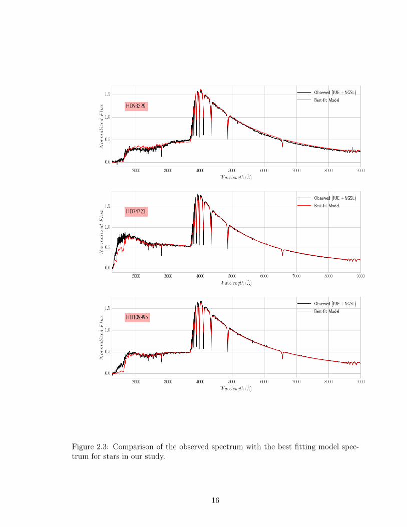
Figure 2.3: Comparison of the observed spectrum with the best fitting model spec-trum for stars in our study.
16

2.5.2 Constructing SED
We used grids of model spectra calculated by Kurucz(2004) in this study. We calculate
synthetic magnitudes based on these spectra for various bands including Johnson U,
B, V, R, I stromgren u, v, b, y and GALEX FUV and NUV.
The standard formula to calculate the synthetic magnitude for particular bandpass
is,
m = �2.5 log(
R �f
�i
�f�S�d�R �
f
�i
�S�d�) + ZP (2.1)
where f� is the flux calculated at the surface of the star, and S� is the response
function for a given passband and integration limits represent the wavelength interval
for a given passband. Response functions for the di↵erent passbands are shown in
Figure 2.4.
As mentioned above all of the stars in our sample have accurate optical photometry
in several bands. For the UV part of the SED we calculated the FUV and NUV
magnitudes using the combined NGSL and IUE spectra.
17

Figure 2.4: Passband response functions from which synthetic magnitudes have beencomputed. All curves are normalized to one, and as shown as function of wavelength.
18

2.5.3 Bayesian Inference
There are many di↵erent codes available for SED fitting and most of them considers
the best-fit model parameters. This method can cause problems when the observa-
tional data covers a large wavelength ranges. Moreover, the errors associated with
the best-fit measurements can be physically meaningless sometimes.
In this study therefore we decided to use the Bayesian approach, for measuring
the goodness of fit between the observed and model data while incorporating the
statistical measurement errors. The key idea here is to obtain a full probability
distribution for a given parameter. The knowledge of the full distribution allows
to estimate meaningful confidence intervals for a given parameter. In addition a
full distribution can be reduced to a point estimate by computing the expectation
value, mode or standard deviation whenever necessary for tabulating or visualizing
purposes.
In Bayesian statistics, the posterior probability distribution p(✓/D) of the true
value of the model parameters ✓ given the observations D is proportional to the
product of likelihood function p(D/✓) and prior p(✓),
p(✓/D) / p(D/✓)p(✓) (2.2)
Here p(✓) encodes any a priori knowledge about the parameters which we wish to
include in our model. It reflects our knowledge of the distribution of the parameters
in the absence of the observations D.
When we don’t have any prior information we can use a flat (or uniform) prior
for all of our parameters. Then we compute the likelihood of observing SED by
assuming normally distributed uncertainties on the observed magnitudes, such that
the likelihood function is given by,
19

p(✓/D) / p(D/✓) = exp(��2red) (2.3)
where,
�2 =X
i
(fobs � fmodel)2
�2i
(2.4)
where i denotes the ith band and the sum is performed over all observed photo-
metric bands of the star being fitted. The reduced chi-square, �2red as defined by �2/k,
where k is the degree of freedom: k = n �m. Here n is the number of photometric
measurements and m is the number of free parameters in the model.
Taking the probability Pi = P (✓/D) as weights for each model, the expectation
value for a give parameter can be calculated.
x =
Pi PixiPi Pi
(2.5)
Also, the standard deviation,
�x =
sPi Pi(xi � x)2P
i Pi
(2.6)
2.5.4 SED Fitting Results
We computed the posterior probability density for the stars in our sample and exam-
ples of them are shown in Figure 2.5.
20

Figure 2.5: Example posterior joint distribution between Teff and log g for a star inour study. Color bar on right of plot represent the probability.
The whole sample follows the same pattern, where the posterior for log g and
[Fe/H] is typically broad, while that of Teff is relatively tighter.
The final expectation values and standard deviations calculated from these dis-
tributions are shown in Table 2.1.
21

Object Teff (K) log g (dex) [Fe/H] (dex)
HD2857 7450/7560 2.6/2.9 -1.6/-1.1HD74721 8640/8500 3.55/3.3 -1.48/-1.2HD86986 7850/7790 3.1/3.0 -1.5/-1.2HD10995 8000/7900 3.5/3.2 -1.7/-1.2HD93329 8127/8200 2.8/3.1 -1.2/-0.9HD319 8140/8090 4.3/3.7 -0.7/-0.9HD60778 8100/8130 2.7/3. -1.4/-1.1
Table 2.1: Stellar parameters obtained from SED fitting compares to published values(column format is published/SED fitting)
As shown in the Table 2.1 , our temperature values agree quite well with the high
resolution spectroscopic measurements. The log g and [Fe/H] values are not as accu-
rate as Teff values, and has average scatter about 0.3 dex compare to the published
values. But the broader probability distribution in these parameters causes signifi-
cantly larger errors in log g and [Fe/H]. Typical errors are 150 K for temperature
and 0.6 dex for log g and [Fe/H].
2.6 Summary
In this section, we evaluate the consistency between observed energy distribution of
metal-poor A-type stars and that of Kurucz(ATLAS12) models, especially focusing on
the UV wavelengths. We noticed that the observed and model energy distributions
agreed quite well overall, with slight deviation at far-UV wavelengths. We have
estimated that the model fluxes below 2000 A predict less flux than the observed
flux.
In addition we measured the stellar parameters for these stars following a Bayesian-
like probability SED fitting procedure. The purpose of this method was to use the all
available flux data from UV to IR, while considering the statistical significance of the
full model parameter space. The method successfully predict the temperature values
but there is significant scatter in surface gravity and metalicity measurements. This
22

suggests that the method is not very successful in breaking the degeneracy between
parameters. However, we emphasize the most useful aspect of the Bayesian inference
is the ability to incorporate pre-known information (prior) to the calculations. In our
method we treated all the parameters with equal probability (flat priors). By using
appropriate priors for the parameters can in principle break the degeneracies between
parameters and give more accurate estimates.
23

Chapter 3 Blue Straggler Stars in the Galactic Field
3.1 Introduction
3.1.1 Blue Straggler Stars
Blue Straggler stars were first discovered in a photometric study of globular cluster
M3 by Sandage in 1953. [22]. They are identified by there position in color magnitude
diagram, in which they appear along the extension of the main sequence but more
bluer and brighter than the main sequence turn-o↵ and apparently younger than the
most of the stellar population. The BSS sequence is a typical feature of most of the
globular clusters.(Figure 2.1) Moreover, since Sandages discovery blue stragglers have
been observed in many stellar environments,like , open clusters [23] , globular clusters
[24], dwarf spheroidal galaxies [25] and galactic field.[26]
Interestingly, the single stellar evolutionary theory failed at explaining the exis-
tence of BSS sequence in CMD of steller populations. Even though exact mechanism
of the formation of blue stragglers is not fully understood there are two theories pop-
ular among astronomers . Both theories rely on the basic idea that BSS are formed
by adding mass to a main sequence star in a binary or multiple stellar system via
some mechanism.
(1) Merger between stellar systems
This could happen in many scenarios: merger of a contact binary, merger during
a dynamical encounter and a merger of an inner binary in hierarchical triple sys-
tem. Direct stellar collision will result in a slower rotating BSS. Binary coalescence,
however, will result in a faster rotating object (if the pair is of similar mass).
(2) Mass transfer between two stars in a binary system.
This is the case where the more massive star in a binary system transfers material,
24

Figure 3.1: Observed CMD for M67. The axes are the color and magnitude labeledwith the central wavelengths. The pentagonal points are the blue stragglers more lu-minous than the main-sequence turno↵, the squares the intermediate-color stragglersand clump giants, including one possible AGB star.Adopted from [27]
during its post main-sequence phase,to its companion star. If the mass transfer is
stable, this may add su�cient mass to the secondary to convert it into a blue straggler.
This appears to be the main formation channel for BSS.
By comparison, BSS formation via the mechanisms involving single stars were
25

either discredited or believed to be much rarer. Some of the interesting ideas related
to single star BSSs are : delayed or late star evolution, extended main sequence
lifetimes due to large scale mixing [28] , highly evolved stars that happened to land
close to the normal main sequence and tidal capturing of young Galactic field stars.
3.1.2 Mass Transfer via Roche-Lobe Overflow
The Roche lobe is the region around a star in a binary system within which orbiting
material is gravitationally bound to that star. It is an approximately circular-shaped
region bounded by a critical gravitational equipotential, with the apex of the tear
drop pointing towards the other star (the apex is at the L1 Lagrangian point of the
system). When the radius of a star in a binary system becomes larger than its Roche-
Lobe, it will transfer mass to its companion star as shown Figure 3.2. This mechanism
is called Roche lobe overflow (RLOF). It was one of the first models suggested for
the origin of BSS [29].
In a cluster of stars , when the accretor is a main sequence star and accrete enough
material to increase its mass above that of the cluster turno↵, a blue straggler is
formed.
The product of binary mass transfer depends on several characteristics of the
system:
1. the evolutionary status of the donor : this implies its complete internal struc-
ture
2. the structure of the donor envelope
3. the mass ratio of the binary
4. the type of the accretor
The nature of all these properties are responsible for the stability of the mass
transfer and for its final product.
26

Figure 3.2: The evolutionary pathway to produce blue straggler stars (BSSs) throughmass transfer. First the bigger primary evolves o↵ the main sequence and fills itsRoche lobe. Then secondary gains mass from the primary becoming a BSS
Generally the mass transfer binaries are classified on the basis of what state of
evolution the donor is in ([30])
Case A: during hydrogen burning in the core of the donor.This can happen if
the orbital separation of the binary is small (usually a few days).
Case B: after exhaustion of hydrogen in the center of the donor (red giant phase).
In this case orbital period is less than about 100 days, but longer than a few days.
Case C: after exhaustion of central helium (He) burning (AGB phase). Here the
orbital period is above 100 days.
It is believed that Case A mass transfer is more likely to be result in the coelescense
of the two stars.(for example [31]) In that sense it can be treated as one of the
merger scenarios. According to the binary evolution simulations ([31] etc.), in order to
produce a BSS via Case B and Case C, the mass transfer has to stable. During stable
27

mass transfer the donor stays within its Roche-lobe. Therefore the stability of the
mass transfer depends on donors response to the mass loss and on how conservative
the process is and what are angular momentum loss processes in this binary.
Given stable mass transfer, case B mass transfer leaves a He white dwarf compan-
ion bound to the blue straggler, while Case C mass transfer leaves a CO white dwarf
companion.
3.1.3 Field Blue Straggler Stars
For given stellar population the dominant formation channel of BSSs depends on its
environment. The BSS in galactic field, where the stellar number density is much
lower than globular clusters, were formed primary due to mass transfer [26]. High
resolution study of Field BSS done by Preston an Sneden [26] suggested that 60
% their sample were binaries. Moreover they concluded that the great majority of
field BSSs probably created by Roche-lobe overflow during red giant branch evolution
(Case B). Ryan et. al. ([32])studied lithium deficiency and rotation of the BSS and
came to the conclusion that these stars can be regard as mass transfer binaries.
The origin of BSS in the Galactic field is related to the formation of the Galactic
halo as well. In addition to the idea of in situ origin, Preston ([33]) argued that
modest fraction of BSS could be a stellar population belong to an accreted Galactic
satellites similar to Carina dSph.
While we have an overall understanding of how blue stragglers could be formed
via di↵erent mass transfer mechanisms, stellar evolution theory is far from predicting
the exact nature and the frequencies. To test the theory with observations, it is vital
to identify the clean sample of mass transfer candidates. Since blue stragglers in
globular clusters are contaminated by those formed via collisions, blue stragglers in
a field are the best candidates for a clean sample of mass-transfer BSS.
As mentioned in the last section the mass-transfer process result in BSS with a
28

white dwarf companion. BSS are much brighter than WDs at optical wavelengths so
,such binaries are hard to find. But if the WD companions to BSS are young and
hot, they can be detected at ultraviolet wavelengths. This opens the possibility to
detect the mass transfer formation of BSS.
3.1.4 White Dwarf Stars
White dwarfs are the end product of stellar evolution for the low-intermediate mass
main sequence stars. In fact, more than 95 % of all stars are expected to end their
lives as white dwarfs. In white dwarfs gravitational collapse in prevented by the
pressure of degenerate electrons, rather than the thermo-nuclear reactions. One of
the key features of white dwarfs is the cooling sequence, i.e. white dwarfs decrease
their luminosity as they age.
Based on the composition of the thin atmosphere, white dwarfs classified into
several types. White dwarfs that have hydrogen dominated atmospheres are called
DA white dwarfs, while white dwarfs have helium dominated atmospheres are called
DB. DA white dwarfs are the most common type. There gravity is so strong such that
all the heavy elements are sinked down below the visible layers. This will create a
thin pure hydrogen atmosphere in the white dwarf. In hot (young) white dwarfs this
sedimentation process happens happens very quickly because the di↵usion time scales
are only of the order of days. In the case of DB white dwarfs (pure He atmospheres),
the outer H layer has been completely lost, and He as the next lightest element floats
up to the top.
A small number of white dwarfs (less than 10 % of total WD observed) are com-
posed of di↵erent elements in their atmospheres, such as C (DQ) and other heavy
elements (DZ). Hot white dwarf atmospheres composed of ionized He are called DO,
and cool stars which show no identifiable features are labelled as DC.
Pre-white dwarf atmospheres are mainly composed of He and/or a mixture of C,
29

N and O, or H depending on the previous evolution from the MS. The H-rich stars
remain their whole lives as DA. He- and CNO-rich stars initiate their life as hot DO
and the di↵usion of heavy elements is supposed to leave behind a surface of H as
they cool. Below Te↵ < 10000 K, the chemical evolution of the WD becomes more
complicated and is not fully understood.
This chapter focuses on the detecting the mass transfer field BSSs from the SDSS
survey and use them to characterize the formation histories.
3.2 Analysis
3.2.1 Identification of Field Blue Straggler Stars
The stellar population in Galactic field is di↵erent from the other two principal Galac-
tic populations, thick and thin discs. While the stars in the halo field are old and
metal poor the stars in discs are young and metal rich. But separation of these
populations is not easy because the distributions overlap.
Over the years many photometric studies have been done to identify field BSS,
primarily using color-color plots. For example Yanni et. al ([34]) identified 2700 field
BSSs using SDSS photometry . Sirko et. al used SDSS photometry in combination
with spectroscopy to identify field BSSs ([35]).
The data used for this study were taken from the Sloan Digital Sky Survey Data
Release 12 (SDSS DR12) and Galaxy Evolution Explorer (GALEX) GR5, an ultra-
violet survey.
3.2.2 SDSS Data
SDSS is an optical photometric and spectroscopic survey that obtains its data from a
2.5 m telescope in Apache observatory in New Mexico. SDSS DR12 o↵ers the latest
data from SDSS project 3. It provides photometry in 5 bands (u, g, r, i and z)
for 400 million objects spanning a magnitude range 15-22 and covering 11500 deg2,
30

approximately quarter of the celestial sphere. The detection limit for point sources
with 1 arcsecs seeing is 22.3, 23.3, 23.1, 22.3 and 20.8 magnitudes on the AB system
respectively, at an air mass of 1.4. Also DR12 includes low resolution spectroscopy
with resolution R 1800 and wavelength coverage 3800-9200A, for about 2 million
objects.
Using the SDSS photometry field BSSs can be identified using the u-g vs g-r
color-color plot using the following color cuts.(Figure 3.3)
0.60 < (u� g) < 1.60 (3.1)
�0.20 < (g � r) < 0.05 (3.2)
This area in the color-color diagram is populated by A-type stars including high
gravity BSS and low gravity BHB stars. Therefore, in order to separate the BSS from
BHB stars one would need stellar parameters for individual stars. For that purpose
we employed the current version of the Extension for Galactic Understanding and
Exploration (SEGUE) Stellar Parameter Pipeline (SSPP) [37].
SSPP uses 8 primary methods for the estimation of e↵ective temperature, Teff ,
10 for the estimation of logg and 12 for the estimation of [Fe/H]. Typical errors for
the SSPP measurements are, �(Teff ) = 200K, �(logg) = 0.4dex, and �([Fe/H]) =
0.3 dex (These evaluations are for the stars that have spectra signal to noise ratio
(S/N = 25), so these errors increase as the S/N decreases.)
The stars selected via the initial color cut using equation 3.1 and 3.2 were plotted
in Teff � log g plane as shown in Figure 3.4. The two sequences of low gravity BHB
and high gravity BSS are clearly visible in the logg vs Teff diagram. We select only
the BSSs above 7000 K to avoid contamination of other F,G type main sequence stars
and/or variable RR lyrae stars.
31

Figure 3.3: The color selection in u-g and g-r used to select BHB and BS stars.Adopted from Xue et.al. [36]
3.2.3 GALEX Data
The Galaxy Evolution Explorer (GALEX) was a NASA Small Explorer mission 1,
all-sky ultraviolet survey conducted from 2003-2013. It was performed in two ul-
traviolet(UV) bands Far-UV(FUV) and Near-UV(NUV). (Figure 3.5) The e↵ective
wavelengths are 1516 and 2267 angstroms for FUV and NUV bands respectively. It
consists of 0.5 m diameter modified Ritchey-Cheretien telescope which has a wide
1.25 degree filed of view and simultaneous imaging coverage in the FUV and NUV.
The image resolution of the instrument is 4.2” in the FUV band and 5.3” in the NUV
band. With pixels 1.5”, this translates to FWHM of approximately 2. pixels in the
1See http://www.galex.caltech.edu for more information.
32
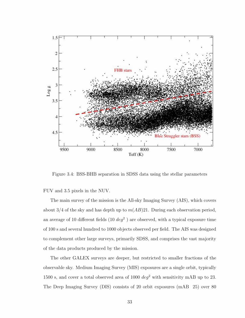
Figure 3.4: BSS-BHB separation in SDSS data using the stellar parameters
FUV and 3.5 pixels in the NUV.
The main survey of the mission is the All-sky Imaging Survey (AIS), which covers
about 3/4 of the sky and has depth up to m(AB)21. During each observation period,
an average of 10 di↵erent fields (10 deg2 ) are observed, with a typical exposure time
of 100 s and several hundred to 1000 objects observed per field. The AIS was designed
to complement other large surveys, primarily SDSS, and comprises the vast majority
of the data products produced by the mission.
The other GALEX surveys are deeper, but restricted to smaller fractions of the
observable sky. Medium Imaging Survey (MIS) exposures are a single orbit, typically
1500 s, and cover a total observed area of 1000 deg2 with sensitivity mAB up to 23.
The Deep Imaging Survey (DIS) consists of 20 orbit exposures (mAB 25) over 80
33

Figure 3.5: Transmission curves for GALEX bandpasses
deg2 and is designed to overlap with existing multiwavelength coverage.
3.2.4 Cross-Identification of sources
Most GALEX observations are designed to cover regions of the sky already observed
by the SDSS at a comparable depth (Figure 3.6).
In order to construct spectral energy distributions(SED) from UV to IR requires
to linking SDSS sources to GALEX counterparts. The matching was done online
using the CDS X-Match Service 2, adopting a match radius of 5” . Such a match
highly depends on the positional accuracy and resolution of both surveys. Because
the GALEX images have lower angular resolution, we tallied instances of multiple
2http://cdsxmatch.u-strasbg.fr/xmatch
34
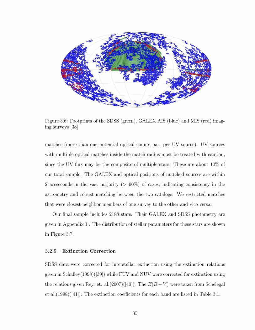
Figure 3.6: Footprints of the SDSS (green), GALEX AIS (blue) and MIS (red) imag-ing surveys [38]
matches (more than one potential optical counterpart per UV source). UV sources
with multiple optical matches inside the match radius must be treated with caution,
since the UV flux may be the composite of multiple stars. These are about 10% of
our total sample. The GALEX and optical positions of matched sources are within
2 arcseconds in the vast majority (> 90%) of cases, indicating consistency in the
astrometry and robust matching between the two catalogs. We restricted matches
that were closest-neighbor members of one survey to the other and vice versa.
Our final sample includes 2188 stars. Their GALEX and SDSS photometry are
given in Appendix 1 . The distribution of stellar parameters for these stars are shown
in Figure 3.7.
3.2.5 Extinction Correction
SDSS data were corrected for interstellar extinction using the extinction relations
given in Schafley(1998)([39]) while FUV and NUV were corrected for extinction using
the relations given Rey. et. al.(2007)([40]). The E(B�V ) were taken from Schelegal
et al.(1998)([41]). The extinction coe�cients for each band are listed in Table 3.1.
35

Figure 3.7: Stellar parameter distributions for filed BSSs selected in this study
3.2.6 UV-Excess Stars
The optical CMDs are usually dominated by the cool stars so that the characterization
BSSs or other hot stars like extreme blue horizontal branch or the binary star products
is di�cult. In addition BSSs can be easily mimicked by photometric blends of sub-
giant branch (SGB) and red giant branch (RGB) stars in the optical CMD. Therefore
UV colors must be used to identify the special features of the BSSs.
36
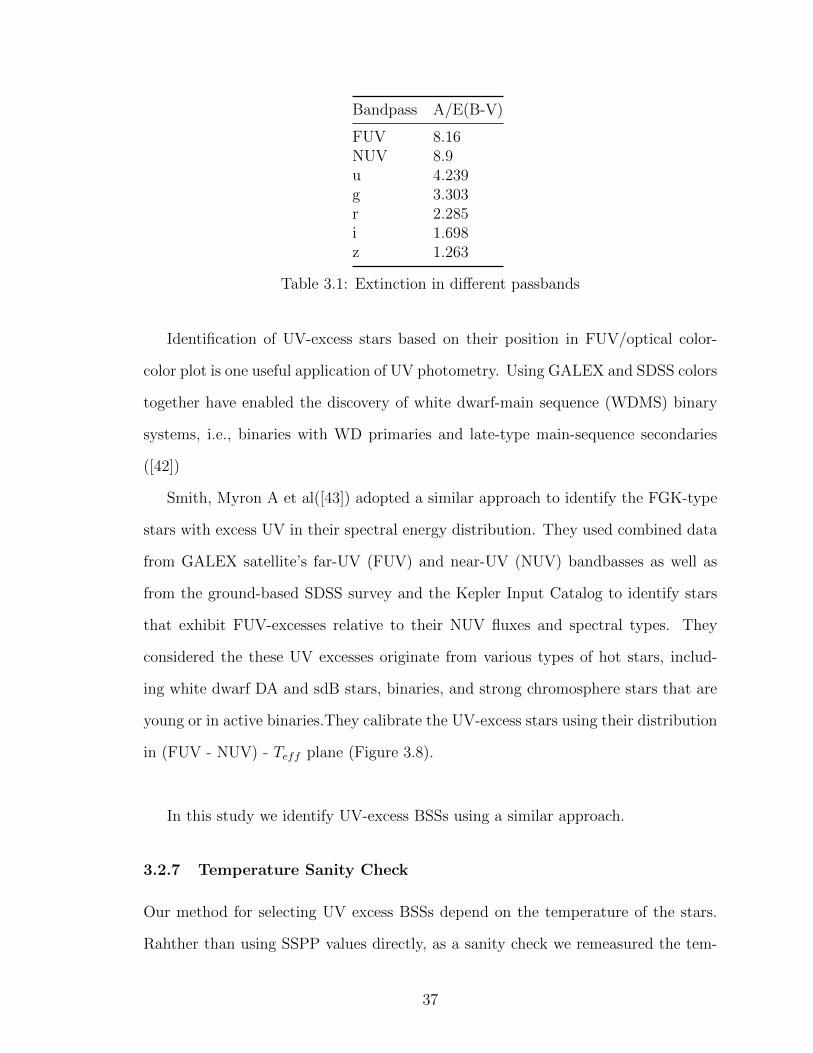
Bandpass A/E(B-V)
FUV 8.16NUV 8.9u 4.239g 3.303r 2.285i 1.698z 1.263
Table 3.1: Extinction in di↵erent passbands
Identification of UV-excess stars based on their position in FUV/optical color-
color plot is one useful application of UV photometry. Using GALEX and SDSS colors
together have enabled the discovery of white dwarf-main sequence (WDMS) binary
systems, i.e., binaries with WD primaries and late-type main-sequence secondaries
([42])
Smith, Myron A et al([43]) adopted a similar approach to identify the FGK-type
stars with excess UV in their spectral energy distribution. They used combined data
from GALEX satellite’s far-UV (FUV) and near-UV (NUV) bandbasses as well as
from the ground-based SDSS survey and the Kepler Input Catalog to identify stars
that exhibit FUV-excesses relative to their NUV fluxes and spectral types. They
considered the these UV excesses originate from various types of hot stars, includ-
ing white dwarf DA and sdB stars, binaries, and strong chromosphere stars that are
young or in active binaries.They calibrate the UV-excess stars using their distribution
in (FUV - NUV) - Teff plane (Figure 3.8).
In this study we identify UV-excess BSSs using a similar approach.
3.2.7 Temperature Sanity Check
Our method for selecting UV excess BSSs depend on the temperature of the stars.
Rahther than using SSPP values directly, as a sanity check we remeasured the tem-
37

Figure 3.8: (FUV-NUV) vs. SDSS/DR7 Te↵ values from GALEX-SDSS data. Sym-bols denote 1 kK bins in Te↵. Solid symbols denote the stars used to define theupper (FUV-NUV) - Te↵ diagonal sequence and calibrate this color from their Te↵values. The dot-dashed locus separates the calibration sequence from the UV-excesspopulation in the lower left. [43]
peratures for our sample by fitting of the Hydrogen balmer lines of the SDSS spec-
trum to model spectrum. For that purpose we created the synthetic spectra using
SPECTRUM package ([21]). SPECTRUM synthesizes stellar spectra assuming a
plane-parallel atmosphere geometry and local thermal equilibrium (LTE).
38
We adopted Kurucz ATLAS12 atmosphere models.3 In order to achieve a more
dense grid of spectra we interpolate the Kurucz models using kmod IDL package.4.
kmod interpolates linearly a Kurucz model for the desired values of e↵ective tem-
perature, surface gravity and metallicity using 8 surrounding models. Our final grid
consists of spectra with the temperatures in the range 6500 - 10,000 K in steps of 125
K.
The final temperatures were estimated using the Bayesian formalism describe in
section 2.3. Note here we fit the spectral absorption line, rather than photometric
point, therefore our degree of freedom is equal to the number of pixels in a given
line(or the number of wavelength data points). Since we used H � ↵ and H � �
lines in our fitting, we we multiply the individual likelihood to get the final posterior
probability. Finally the point estimates of mean and error in temperatures were
calculated.The mean error obtained for temperatures is 140 K.
We compared the temperatures obtained from our method to those obtained from
the SSPP in order to check the consistency (Figure 10). Both SSPP and our method
predicts consistent values for majority of the stars. Given the uncertainties in our
measurements we continue our analysis with the all the stars except the ones with
Teff di↵erence larger than 250 K. For the rest of the analysis we consider only the
SSPP values.
3Kurucz models are available at http:kurucz.harvard.edu
4http://www.as.utexas.edu/ hebe/
39

Figure 3.9: Comparison of temperatures of BSSs in this work with SSPP
We plotted Te↵ values determined from the SSPP vs FUV � NUV color of the
stars in our sample (Figure 3.10). The diagonal sequence in the Figure 3.10 reflects
the relationship between SDSS Teff and FUV � NUV for the main-sequence stars.
We fit the main diagonal sequence with a quadratic fit and the stars lying outside the
2� from the best fit were selected as UV-excess BSS stars. These are our candidates
for the BSS with a hot WD companion.
40

Figure 3.10: (FUV-NUV) vs. SSPP temperature values from SDSS-GALEX data.The red dashed line is the 2� deviation from the fit to the diagonal sequence. Starslocated left to this line are BSS with UV-excess.
3.2.8 BSS-WD Fitting
In order to obtain the stellar parameters of BSS-WD binaries, we fit the observed
SED of UV-excess stars with a composite model SED consists of BSS and white
dwarf. We employed theoretical grid of spectra developed by Kurucz(2004), in which
the e↵ective temperature, Teff covers a range from 6000 to 10000 in steps of 250
K, and the surface gravity, logg covers a range from 0.5 to 5. in steps of 0.5, and
metallicity, [Fe/H] covers a range from -2.5 to 0.5 in steps of 0.5. In order to use our
SED fitting routine, model spectra were converted to bandpass fluxes, as explained
in next section.
For white dwarf models we employed the theoretical color tables developed by
Bergeron( University of Montreal; private communication). For these models stellar
41
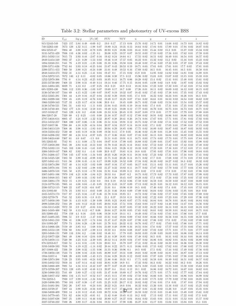
Table 3.2: Stellar parameters and photometry of UV-excess BSS
ID Teff log g [Fe/H] FUV NUV u g r i z
915-52443-549 7423 157 3.84 0.49 -0.69 0.2 19.0 0.17 17.13 0.04 15.76 0.02 14.71 0.01 14.68 0.02 14.73 0.01 14.82 0.02740-52263-440 7673 129 4.32 0.15 -1.98 0.07 19.89 0.24 19.35 0.13 18.64 0.02 17.84 0.01 17.89 0.01 17.94 0.02 18.07 0.03684-52523-47 7004 40 3.88 0.23 -0.78 0.05 20.93 0.21 18.06 0.03 16.41 0.03 15.44 0.02 15.3 0.01 15.27 0.02 15.34 0.023131-54731-429 7936 110 4.36 0.03 -1.35 0.1 20.08 0.25 19.57 0.07 18.55 0.03 17.53 0.02 17.56 0.01 17.62 0.01 17.59 0.032951-54592-114 7615 73 3.93 0.44 -2.07 0.16 19.42 0.24 18.64 0.1 17.55 0.02 16.51 0.02 16.49 0.01 16.54 0.01 16.57 0.022849-54454-349 7083 37 4.21 0.29 -1.53 0.02 19.46 0.18 17.57 0.05 16.22 0.01 15.32 0.02 15.2 0.02 15.16 0.01 15.22 0.021894-53240-211 7441 78 4.19 0.21 -1.25 0.08 21.18 0.26 19.58 0.04 18.48 0.02 17.44 0.02 17.33 0.01 17.37 0.01 17.43 0.022299-53711-626 7742 64 3.93 0.18 -0.25 0.04 21.67 0.43 20.53 0.19 18.71 0.03 17.61 0.01 17.61 0.01 17.7 0.02 17.81 0.032299-53711-453 7460 50 3.88 0.21 -0.24 0.08 21.01 0.48 19.53 0.16 17.69 0.02 16.5 0.01 16.45 0.01 16.5 0.01 16.58 0.012848-54453-473 7032 31 4.14 0.25 -1.41 0.04 19.47 0.1 17.15 0.02 15.9 0.01 14.95 0.02 14.82 0.02 14.81 0.02 14.88 0.011254-52972-515 7672 140 4.2 0.11 -0.02 0.05 18.66 0.38 17.5 0.12 15.96 0.02 15.01 0.01 15.07 0.02 15.15 0.01 15.33 0.011252-52970-306 7791 0 4.14 0.23 -0.25 0.03 16.95 0.11 16.75 0.06 16.28 0.02 15.4 0.02 15.41 0.01 15.48 0.01 15.61 0.022335-53730-480 7468 33 3.98 0.31 -0.49 0.14 19.14 0.46 17.75 0.15 16.04 0.05 14.98 0.02 14.9 0.02 14.97 0.02 15.02 0.023241-54884-335 8029 71 4.13 0.2 -1.97 0.25 19.3 0.21 18.9 0.13 18.16 0.04 17.23 0.02 17.32 0.01 17.42 0.01 17.54 0.02685-52203-430 7686 112 3.93 0.36 -1.03 0.07 19.69 0.17 18.7 0.08 17.26 0.01 16.11 0.02 16.09 0.02 16.12 0.02 16.15 0.023130-54740-107 7344 69 4.15 0.22 -1.89 0.07 19.87 0.19 19.32 0.07 18.45 0.02 17.45 0.02 17.38 0.01 17.35 0.02 17.43 0.022252-53565-281 7301 44 4.19 0.16 -0.27 0.04 21.02 0.39 19.05 0.05 17.4 0.01 16.32 0.02 16.24 0.01 16.26 0.01 16.3 0.011961-53299-168 7291 45 4.05 0.19 -0.76 0.02 19.49 0.17 18.25 0.07 17.61 0.02 16.61 0.01 16.53 0.02 16.54 0.02 16.62 0.021960-53289-343 7127 33 4.23 0.17 -0.54 0.06 20.9 0.4 18.45 0.09 16.71 0.02 15.68 0.02 15.54 0.01 15.54 0.02 15.57 0.023138-54740-521 7381 31 4.03 0.3 -1.11 0.03 21.04 0.45 19.95 0.19 18.44 0.03 17.4 0.01 17.31 0.01 17.35 0.02 17.38 0.023138-54740-401 7562 177 4.31 0.16 -2.59 0.01 19.49 0.21 19.08 0.12 17.77 0.03 16.76 0.01 16.75 0.01 16.73 0.01 16.71 0.021857-53182-27 7343 129 4.31 0.2 -0.88 0.08 21.53 0.34 20.45 0.19 18.87 0.03 17.9 0.01 17.77 0.01 17.79 0.01 17.88 0.03366-52017-28 7320 60 4.2 0.23 -1.01 0.08 21.16 0.37 19.37 0.12 17.88 0.02 16.91 0.02 16.86 0.01 16.86 0.02 16.92 0.022797-54616-614 8005 47 4.24 0.19 -1.22 0.32 20.87 0.38 20.41 0.26 18.74 0.04 17.67 0.01 17.71 0.01 17.81 0.02 17.92 0.032551-54552-257 7368 100 4.07 0.06 -1.31 0.06 21.51 0.34 19.91 0.12 18.75 0.02 17.58 0.02 17.51 0.02 17.52 0.02 17.52 0.032247-53857-96 7290 68 4.18 0.29 -0.54 0.04 20.57 0.34 19.57 0.14 18.18 0.02 17.1 0.02 17.05 0.01 17.08 0.01 17.15 0.022180-54613-519 7368 46 3.98 0.31 -1.83 0.01 20.94 0.29 18.85 0.06 17.75 0.02 16.89 0.02 16.87 0.02 16.87 0.02 16.92 0.021659-53224-452 7530 40 4.05 0.19 -0.56 0.09 19.56 0.15 17.9 0.05 16.46 0.02 15.39 0.01 15.38 0.01 15.45 0.02 15.55 0.022550-54206-232 7097 80 4.24 0.14 -0.97 0.05 21.17 0.36 18.61 0.07 17.16 0.02 16.15 0.01 16.04 0.02 16.02 0.02 16.04 0.022189-54624-640 7307 61 4.0 0.67 -1.5 0.0 21.51 0.45 19.91 0.11 18.71 0.03 17.74 0.02 17.73 0.01 17.75 0.01 17.84 0.03595-52023-92 7542 81 4.11 0.08 -1.72 0.04 19.07 0.18 17.99 0.05 16.88 0.02 15.89 0.01 15.87 0.01 15.92 0.01 15.98 0.021727-53859-288 7045 39 3.84 0.43 -0.53 0.02 21.79 0.43 20.25 0.14 18.61 0.02 17.52 0.02 17.42 0.02 17.42 0.02 17.48 0.022782-54592-113 7445 103 3.88 0.45 -1.61 0.05 19.64 0.21 19.26 0.12 18.33 0.02 17.23 0.01 17.16 0.01 17.12 0.01 17.11 0.023308-54919-447 7368 82 3.92 0.4 -1.41 0.09 20.9 0.37 19.81 0.14 18.8 0.03 17.95 0.02 17.91 0.01 17.96 0.02 18.04 0.032781-54266-417 7768 145 4.37 0.16 -1.34 0.03 20.35 0.26 19.28 0.11 18.16 0.02 17.23 0.02 17.31 0.01 17.34 0.01 17.41 0.022156-54525-520 7483 58 3.89 0.42 -0.98 0.02 21.75 0.42 20.26 0.14 18.71 0.02 17.7 0.01 17.68 0.02 17.74 0.01 17.83 0.023297-54941-411 7411 56 3.98 0.45 -1.14 0.17 19.99 0.28 18.52 0.08 17.34 0.02 16.33 0.02 16.27 0.02 16.3 0.02 16.32 0.022152-53874-290 7557 40 4.14 0.23 -1.02 0.09 19.07 0.16 17.47 0.05 16.17 0.01 15.11 0.02 15.11 0.01 15.17 0.01 15.26 0.023406-54970-104 7191 81 4.32 0.02 -1.98 0.02 21.27 0.32 19.92 0.11 18.77 0.02 17.87 0.02 17.79 0.02 17.77 0.03 17.83 0.023406-54970-518 7335 50 4.25 0.18 -1.79 0.04 21.91 0.44 19.89 0.11 18.8 0.02 17.9 0.02 17.8 0.01 17.82 0.01 17.86 0.033387-54951-106 7979 116 4.21 0.38 -1.84 0.21 20.53 0.4 20.07 0.2 18.75 0.02 17.73 0.02 17.73 0.02 17.87 0.02 17.99 0.023384-54948-315 7403 67 3.89 0.33 -1.92 0.07 21.29 0.28 19.45 0.07 18.29 0.02 17.3 0.02 17.24 0.02 17.25 0.02 17.32 0.021348-53084-179 7652 15 4.19 0.21 -2.24 0.0 19.6 0.18 18.53 0.06 17.59 0.02 16.59 0.01 16.59 0.02 16.67 0.02 16.69 0.022124-53770-535 7005 44 4.08 0.04 -1.45 0.05 21.25 0.45 18.57 0.09 17.13 0.02 16.25 0.01 16.12 0.01 16.12 0.01 16.15 0.012336-53712-115 7469 22 4.07 0.23 -0.6 0.07 21.01 0.4 19.96 0.19 18.5 0.02 17.46 0.02 17.4 0.01 17.45 0.01 17.52 0.02424-51893-60 7176 23 3.93 0.11 -0.61 0.09 21.31 0.46 18.84 0.09 17.09 0.02 16.04 0.02 15.94 0.02 15.95 0.01 16.0 0.022445-54573-173 7317 87 4.25 0.34 -1.37 0.46 21.78 0.34 19.85 0.1 18.72 0.02 17.66 0.02 17.57 0.02 17.65 0.02 17.69 0.021282-52759-79 7541 52 3.83 0.35 -1.8 0.13 21.1 0.37 19.53 0.11 18.32 0.02 17.22 0.03 17.23 0.01 17.29 0.01 17.36 0.023377-54950-189 7349 31 4.13 0.35 -1.38 0.09 19.95 0.21 18.83 0.07 17.75 0.02 16.84 0.01 16.78 0.01 16.81 0.02 16.84 0.022899-54568-252 7164 29 4.01 0.12 -0.22 0.05 20.04 0.23 17.51 0.04 15.63 0.03 14.57 0.02 14.46 0.02 14.47 0.01 14.56 0.021456-53115-620 7072 59 3.9 0.27 -0.84 0.04 21.53 0.48 18.97 0.05 17.32 0.02 16.22 0.02 16.14 0.02 16.18 0.02 16.24 0.022661-54505-400 7402 59 4.13 0.12 -0.7 0.08 20.64 0.27 18.93 0.05 17.65 0.02 16.61 0.02 16.59 0.01 16.62 0.01 16.71 0.01335-52000-452 7758 159 4.1 0.16 -2.03 0.06 19.58 0.19 19.11 0.1 18.49 0.02 17.54 0.02 17.61 0.01 17.66 0.01 17.7 0.022647-54495-235 7096 51 3.9 0.12 -1.47 0.02 21.61 0.42 19.04 0.09 17.62 0.02 16.66 0.02 16.56 0.02 16.55 0.02 16.59 0.023253-54941-210 7296 41 3.96 0.27 -1.74 0.04 21.47 0.47 19.29 0.07 17.99 0.02 17.06 0.02 17.0 0.02 17.03 0.02 17.08 0.02334-51993-267 7270 74 3.94 0.28 -1.38 0.01 21.78 0.41 20.32 0.13 18.76 0.02 17.7 0.02 17.63 0.02 17.66 0.01 17.71 0.023214-54866-426 7159 49 3.85 0.3 -1.68 0.04 21.69 0.48 19.99 0.16 18.55 0.04 17.6 0.02 17.57 0.02 17.55 0.02 17.61 0.022892-54552-128 7256 80 3.84 0.37 -1.99 0.13 22.22 0.3 19.94 0.08 18.67 0.02 17.82 0.02 17.71 0.01 17.71 0.01 17.77 0.023285-54948-131 7509 116 3.94 0.2 -1.66 0.02 18.48 0.1 17.79 0.05 16.93 0.03 15.98 0.03 16.03 0.03 16.06 0.02 16.14 0.032512-53877-326 7061 48 3.86 0.16 -2.04 0.09 21.44 0.38 18.85 0.04 17.48 0.02 16.5 0.01 16.41 0.02 16.44 0.01 16.46 0.023170-54859-111 7520 98 4.23 0.31 -2.39 0.05 20.12 0.14 18.93 0.04 17.87 0.02 16.86 0.01 16.82 0.01 16.84 0.02 16.89 0.02878-52353-617 7240 51 4.14 0.31 -1.81 0.16 20.61 0.3 18.79 0.07 17.41 0.02 16.44 0.02 16.33 0.02 16.36 0.03 16.38 0.023193-54830-593 7838 78 4.19 0.22 -1.14 0.02 20.44 0.22 19.71 0.11 18.66 0.03 17.55 0.02 17.62 0.01 17.66 0.02 17.75 0.03267-51608-422 7336 59 3.98 0.32 -1.55 0.06 21.55 0.36 19.96 0.1 18.5 0.02 17.5 0.02 17.44 0.02 17.49 0.02 17.56 0.031739-53050-128 7533 73 3.98 0.16 -2.23 0.05 20.89 0.37 19.31 0.08 18.01 0.02 16.98 0.02 16.81 0.01 16.87 0.02 17.13 0.021934-53357-4 7408 39 4.03 0.09 -1.43 0.15 21.64 0.28 20.35 0.12 19.02 0.03 17.97 0.03 17.95 0.02 17.98 0.02 18.02 0.041590-52974-388 7126 23 3.95 0.05 -0.24 0.02 21.86 0.46 19.31 0.1 17.71 0.02 16.58 0.01 16.49 0.02 16.51 0.02 16.57 0.023195-54832-552 7059 34 4.07 0.14 -0.42 0.03 20.81 0.39 18.9 0.1 17.32 0.02 16.3 0.02 16.22 0.02 16.2 0.01 16.26 0.013230-54860-409 7081 54 4.34 0.14 -0.42 0.07 20.77 0.37 18.49 0.08 16.74 0.02 15.65 0.02 15.55 0.02 15.58 0.02 15.63 0.022273-53709-207 7353 128 4.05 0.32 -0.48 0.13 20.97 0.4 19.41 0.12 18.1 0.02 16.86 0.02 16.72 0.01 16.67 0.01 16.62 0.013230-54860-353 7541 69 3.89 0.27 -1.52 0.05 21.47 0.49 19.89 0.17 18.76 0.02 17.75 0.01 17.71 0.02 17.77 0.02 17.84 0.023226-54857-452 8004 116 4.15 0.17 -0.52 0.17 18.15 0.11 17.89 0.02 17.58 0.02 16.66 0.01 16.74 0.01 16.86 0.01 16.99 0.02758-52253-5 7930 117 3.99 0.18 -1.34 0.04 18.47 0.12 18.45 0.04 18.45 0.03 17.75 0.02 17.79 0.02 17.92 0.01 18.05 0.032420-54086-395 7780 101 4.07 0.38 -1.47 0.05 21.25 0.35 20.17 0.12 18.82 0.02 17.84 0.01 17.8 0.01 17.87 0.01 17.94 0.022541-54481-384 7282 26 3.87 0.0 -0.24 0.01 20.22 0.21 18.0 0.04 16.32 0.02 15.26 0.01 15.16 0.03 15.17 0.02 15.25 0.022055-53729-37 7297 44 3.99 0.25 -0.56 0.05 19.97 0.17 17.86 0.04 16.37 0.01 15.32 0.02 15.26 0.0 15.27 0.01 15.35 0.013166-54830-409 7203 14 4.18 0.12 -0.45 0.03 20.72 0.34 18.28 0.07 16.59 0.02 15.55 0.01 15.46 0.01 15.49 0.02 15.61 0.023161-54779-445 7351 62 4.04 0.23 -0.81 0.1 21.42 0.48 19.45 0.13 18.2 0.02 17.13 0.02 17.11 0.01 17.22 0.02 17.3 0.022941-54507-638 7097 25 4.09 0.11 -0.46 0.02 20.89 0.27 18.37 0.04 16.64 0.02 15.65 0.01 15.51 0.01 15.52 0.01 15.57 0.022337-53740-222 7100 26 3.89 0.17 -0.24 0.04 19.51 0.17 17.98 0.06 16.27 0.01 15.17 0.01 15.04 0.01 15.04 0.01 15.1 0.01
42

masses and cooling ages are obtained from a detailed evolutionary cooling sequences
appropriate for these stars. For the white dwarfs with pure hydrogen model atmo-
spheres above temperatures = 30,000 K, the carbon-core cooling models of Wood
([44]) with thick hydrogen layers of MH/M⇤ = 104 were used. For temperatures
below 30,000 K, cooling models similar to those described in Fontaine, Brassard,
& Bergeron et. al ([45]) but with carbon-oxygen cores and MH/M⇤ = 104 were
used. For the pure helium model atmospheres, similar models being used but with
MH/M⇤ = 10�10.5
3.2.9 Synthetic Fluxes
In the course of fitting procedure we calculate synthetic fluxes for both BSS and WD
in GALEX and SDSSS bandpasses. The synthetic spectra can be converted to a
monochromatic flux for a given bandpass via,
f =
R �f
�i
�f�S�d�R �
f
�i
�S�d�(3.3)
where f� is the flux at a given wavelength � and S� is the filter response at a given
wavelength. The integration limits are the minimum and maximum wavelength of
the bandpass.
3.2.10 Observed Fluxes
The observed, extinction corrected, magnitudes were transformed to fluxes using the
standard formulas. For SDSS bandpasses,
mAB = �2.5 log f⌫ � 48.6 (3.4)
5see Bergeron, Leggett, & Ruiz 2001, ApJS, 133, 413 for more details
43
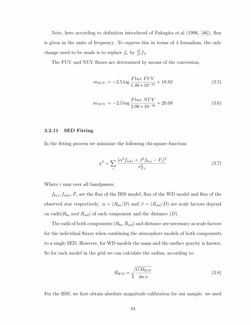
Note, here according to definition introduced of Fukugita et.al (1996, [46]), flux
is given in the units of frequency. To express this in terms of � formalism, the only
change need to be made is to replace f⌫ by �2
c2f�.
The FUV and NUV fluxes are determined by means of the conversion,
mFUV = �2.5 logFlux FUV
1.40 ⇤ 10�15+ 18.82 (3.5)
mNUV = �2.5 logFlux NUV
2.06 ⇤ 10�16+ 20.08 (3.6)
3.2.11 SED Fitting
In the fitting process we minimize the following chi-square function:
�2 =X
i
(↵2fwd,i + �2fbs,i � Fi)2
�2F,i
(3.7)
Where i sum over all bandpasses.
fbs,i, fwd,i, Fi are the flux of the BSS model, flux of the WD model and flux of the
observed star respectively. ↵ = (Rbs/D) and � = (Rwd/D) are scale factors depend
on radii(Rbs and Rwd) of each component and the distance (D).
The radii of both components (Rbs, Rwd) and distance are necessary as scale factors
for the individual fluxes when combining the atmosphere models of both components
to a single SED. However, for WD models the mass and the surface gravity is known.
So for each model in the grid we can calculate the radius, according to:
RWD =
sGMWD
gWD
(3.8)
For the BSS, we first obtain absolute magnitude calibration for our sample. we used
44

transformation equations given in Zhao & Newberg(2006, [47]), which were derived
from the SDSS stars with known UBVRI photometry, including a sample of BSS
stars.
V = g � 0.561(g � r)� 0.004 (3.9)
(B � V ) = 0.916(g � r) + 0.187 (3.10)
These transformations are valid within the range �0.5 < g � r < 1.0,([48]) which
is consistent with the color range we adopted here.
Using the V magnitude we obtained from Equation 3.9, we can now calculate the
absolute magnitude in V band (Mv)using the relation given in Kinman et al.(1994,
[49]):
Mv = 1.32 + 4.05(B � V )� 0.45Fe
H
�(3.11)
This relation was constructed by studying the BSSs in globular clusters with
di↵erent metallicities covering a wide range of colors and absolute magnitudes.
The luminosity of the star can be then, found by using the Mv and bolometric
correction as,
✓L
Lo
◆= 10�0.4[M
v
�Vo
�31.752+(BCv
�BCv,o
)] (3.12)
Where for the bolometric correction we adopt the values given by Torres(2010)
[50] :
Vo = �26.75
BCv,o = �0.09 and
BCv = a+ b(logTeff ) + c(logTeff )2 + ...
45
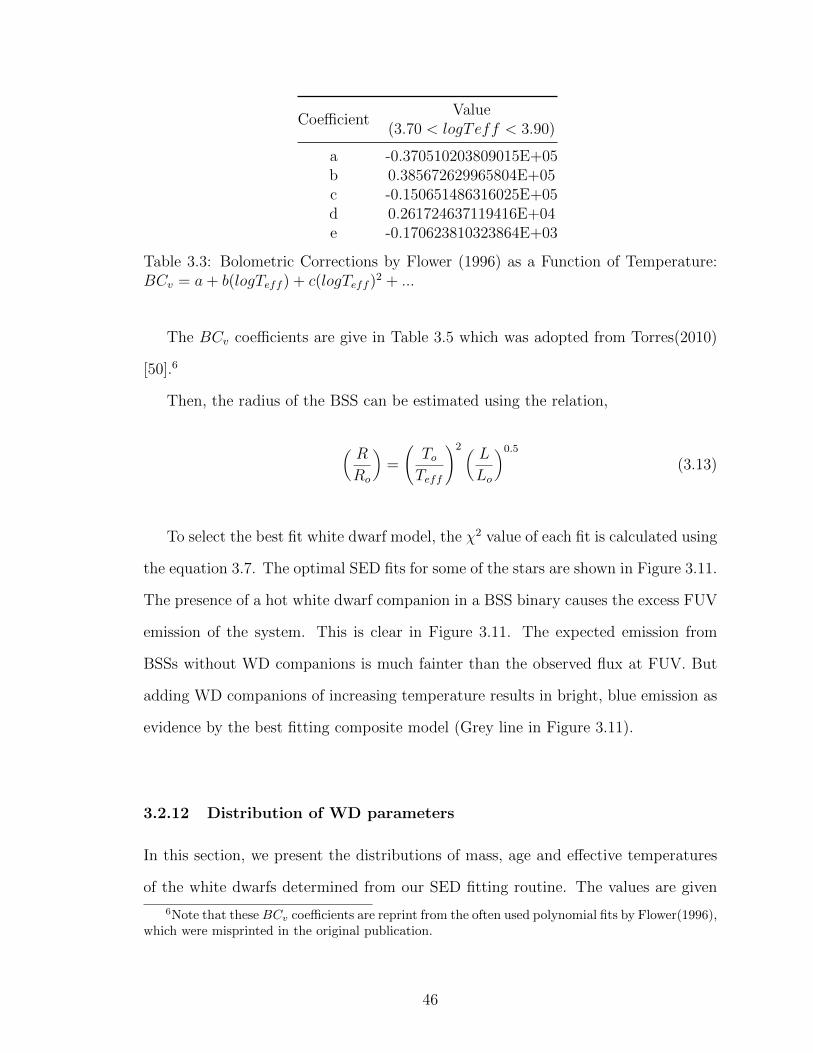
Coe�cientValue
(3.70 < logTeff < 3.90)
a -0.370510203809015E+05b 0.385672629965804E+05c -0.150651486316025E+05d 0.261724637119416E+04e -0.170623810323864E+03
Table 3.3: Bolometric Corrections by Flower (1996) as a Function of Temperature:BCv = a+ b(logTeff ) + c(logTeff )2 + ...
The BCv coe�cients are give in Table 3.5 which was adopted from Torres(2010)
[50].6
Then, the radius of the BSS can be estimated using the relation,
✓R
Ro
◆=
To
Teff
!2 ✓L
Lo
◆0.5
(3.13)
To select the best fit white dwarf model, the �2 value of each fit is calculated using
the equation 3.7. The optimal SED fits for some of the stars are shown in Figure 3.11.
The presence of a hot white dwarf companion in a BSS binary causes the excess FUV
emission of the system. This is clear in Figure 3.11. The expected emission from
BSSs without WD companions is much fainter than the observed flux at FUV. But
adding WD companions of increasing temperature results in bright, blue emission as
evidence by the best fitting composite model (Grey line in Figure 3.11).
3.2.12 Distribution of WD parameters
In this section, we present the distributions of mass, age and e↵ective temperatures
of the white dwarfs determined from our SED fitting routine. The values are given
6Note that these BCv coe�cients are reprint from the often used polynomial fits by Flower(1996),
which were misprinted in the original publication.
46

Figure 3.11: Example of BSS+WD fitting. Orange circles are the observed FUV,NUVand u photometry. Blue and Red lines represent the synthetic spectra of BS(ATLAS9- Kurucz) and WD (Bergeron) respectively.Grey is the combined best fitspectrum for observed photometry.
in table 3.
The most striking features of the distributions are: Vast majority of white dwarfs
are very young (few million years old, See figure 3.11) and with temperatures range
between 20000 - 40000 K (see figure 3.12).
This is consistent with our initial selection criteria of BSS, as recently formed BSS
are expected to have mush larger UV excess.
The white dwarf mass distribution is shown in the bottom panel of figure 3.11.
47

Figure 3.12: White Dwarf parameters
48

One interesting feature of the mass distribution is the peak at white dwarf mass
0.41 M�. White dwarf stars with masses below 0.47 M� are thought to be He-core
white dwarfs. ( Core helium ignition starts when the core mass is roughly 0.47M�)
If these stars were single stars, they would have main sequence life times that are
longer than age of the Universe. Therefore these stars must be a product binary star
evolution.
Only possible scenario for having such low mass white dwarf is case-B binary mass
transfer. At this stage expanding red giant core has not yet fully grown, therefore
the resultant white dwarf will appear with a smaller mass.
On the other hand white dwarfs with masses > .5M� are consistent with theo-
retical predictions from the Case-C mass transfer hypothesis. Case-C mass transfer
(from an asymptotic giant to a main sequence star) leaves a carbonoxygen white
dwarf companion with a mass of about .5 M� -0.6 M� dictated by the core mass of
the asymptotic giant donor at the end of the mass transfer phase ([51]).
The WD Mass distribution in the Galactic field peaks at about 0.59 M� and
exhibits a significant low- mass tail of white dwarfs with masses lower than 0.45
M� which peaks at 0.40 M� ([52]) (Figure 3.13). That white dwarfs predominantly
found in close binary systems, mostly with another white dwarf or a neutron star
companion ([53]). Interestingly, the low mass end of this distribution is consistent
with our results as well.
49

Figure 3.13: This figure adopted from [52] shows the comparison of the SDSS DR7WDmass distributions from their work (black) and Kleinman et al. (2013, filled blue).The low-mass objects (red; M < 0.45 M�) are thought to be the WD originated frombinary mass transfer processes.
The presence of any detected WDs can be used to map out the history of mass
transfer-formed BSSs.
3.2.13 Mass Transfer e�ciency
Mass transfer e�ciency �, which is defined as the mass fraction of the lost mass from
the primary accreted by the secondary, is an important parameter that determines the
character of the BSS. This has been a major issue for the binary evolution calculations.
50

Table 3.4: Stellar Parameters of WD stars
ID WD Te↵ WD mass WD age(My)
915-52443-549 45000.0 0.68 2.81740-52263-440 120000.0 0.7 0.07684-52523-47 20000.0 0.39 31.73131-54731-429 70000.0 0.56 0.572951-54592-114 55000.0 0.51 1.292849-54454-349 30000.0 0.43 9.661894-53240-211 35000.0 0.45 4.592299-53711-626 35000.0 0.45 4.592299-53711-453 25000.0 0.41 16.82848-54453-473 25000.0 0.41 16.81254-52972-515 85000.0 0.6 0.271252-52970-306 120000.0 0.7 0.072335-53730-480 30000.0 0.43 9.663241-54884-335 120000.0 0.7 0.07685-52203-430 70000.0 0.99 0.63130-54740-107 60000.0 0.53 0.962252-53565-281 30000.0 0.43 9.661961-53299-168 65000.0 0.54 0.741960-53289-343 20000.0 0.39 31.73138-54740-521 30000.0 0.43 9.663138-54740-401 55000.0 0.51 1.291857-53182-27 40000.0 0.46 3.1366-52017-28 35000.0 0.45 4.592797-54616-614 60000.0 0.53 0.962551-54552-257 35000.0 0.45 4.592247-53857-96 50000.0 0.5 1.692180-54613-519 35000.0 0.45 4.591659-53224-452 35000.0 0.45 4.592550-54206-232 25000.0 0.41 16.82189-54624-640 50000.0 0.5 1.69595-52023-92 50000.0 0.5 1.691727-53859-288 35000.0 0.45 4.592782-54592-113 50000.0 0.5 1.693308-54919-447 85000.0 0.6 0.272781-54266-417 75000.0 0.57 0.452156-54525-520 40000.0 0.46 3.13297-54941-411 35000.0 0.45 4.592152-53874-290 35000.0 0.45 4.593406-54970-104 35000.0 0.45 4.593406-54970-518 35000.0 0.45 4.593387-54951-106 55000.0 0.51 1.292337-53740-222 30000.0 0.43 9.66
51

Because of its uncertainty most calculations treat it as constant value.([54], [55]). Lu.
p et.al used monte carlo simulations to calculate the models to investigate the origin
of BSSs population in M67. In their calculations they used the � = 0.5 and � = 1.0
(fully conservative mass transfer, i.e. no mass or angular momentum loss from the
system) and found that the higher value could reproduce the data better.
Using the WD parameters we obtained via the BSS-WD fitting can be used to
infer the lower limit of this important parameter.
The amount of mass transferred from the now WD to BSS, �Mt,
�Mtrans = Mi �Mwd (3.14)
where Mi is the progenitor mass of the WD.
We interpolate theoretical relations which were constructed using BaSTI evolu-
tionary models(Pietrinferni et al., 2006([56])) so that we can calculate the progenitor
mass at a given metallicity and age (Figure 3.14).
We adopted the non-canonical BaSTI models with the mass loss e�ciency of
the Reimers law(Reimers 1977) set to ⌘ =0.2. The initial He mass fraction ranges
from 0.245 to 0.303, for the more metal-poor to the more metal-rich composition,
respectively. The adopted BaSTI models cover twelve metallicity bins: Z=0.0001,
0.0003, 0.0006, 0.001, 0.002,0.004, 0.008, 0.0100, 0.0198, 0.0240, 0.0300 and 0.0400.
Jo↵re P. et. al (2011, [57]) estimated the age of the field halo stars using as sample
of SDSS stars. The estimated the mean age 11 giga years, which we adopted in our
calculations to determine the mass from interpolated BASTI models. The field stars
Jo↵re P. et. al used in their study has a metallicity of -1.6 dex. To be consistant
with that work we limited our sample to the stars with [Fe/H] < -1. This reduce
our sample to 35 stars.
Following as similar procedure, we can determine the mass of the BSS MBSS
by using the theoretical relations and the temperature the of the BSS. However to
calculate the amount of mass transferred one would require the initial mass of the
52

Figure 3.14: Theoretical mass-age relations from BaSTI evolutionary models.
secondary star (Now BSS), where the exact value is impossible to infer. But we can
estimate the lower limit of the transferred mass by considering the halo turno↵ mass
of 0.8 M�,
Then the mass accreted on to the secondary (now BSS) is given by,
�Macc = MBSS � 0.8 (3.15)
Now this will give us the lower limit of the mass transfer e�ciency.
The derived � values are shown as cumulative histogram in Figure 3.15. All the
stars have mass transfer e�ciencies above � ⇠ 0.5.
53
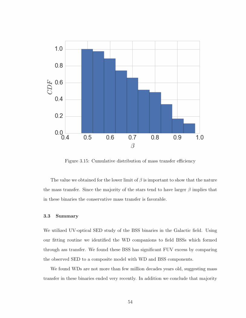
Figure 3.15: Cumulative distribution of mass transfer e�ciency
The value we obtained for the lower limit of � is important to show that the nature
the mass transfer. Since the majority of the stars tend to have larger � implies that
in these binaries the conservative mass transfer is favorable.
3.3 Summary
We utilized UV-optical SED study of the BSS binaries in the Galactic field. Using
our fitting routine we identified the WD companions to field BSSs which formed
through ass transfer. We found these BSS has significant FUV excess by comparing
the observed SED to a composite model with WD and BSS components.
We found WDs are not more than few million decades years old, suggesting mass
transfer in these binaries ended very recently. In addition we conclude that majority
54

of the WDs are helium WDs. The obvious way to produce such low mass stars is via
the mass transfer process of RGB star in a binary system.
Combining the WD stellar parameters with the evolutionary models we estimated
the lower limit of the binary mass transfer e�ciency in these stars to be, � = 0.5.
In order to determine the exact formation mechanisms for a particular population
of BSSs a detailed characterization of the BSSs is needed. This require determining
the rotation velocities and binary orbital parameters. Since the formation channel
for BS binaries can distinguish from the type of companion star expected, it is vital
to identify the observational constraints of the companion. In addition these binaries
will be good test cases for more sophisticated mass transfer modeling e↵orts in the
future.
55

Chapter 4 Canis Major Overdensity
4.1 Introduction
The existence of strong elliptical-shaped stellar overdensity, close to the Galactic plane
at (l = 240, b = 8), in the constellation of Canis Major was identified by Martin et. al
in 2004 ([58]), based on the analysis of red giant stars of the 2 Micron All Sky Survey
(2MASS). They identified the large scale Galactic asymmetry in stellar distribution
above and below the Galactic plane and was first interpreted as a remnant of a
disrupting dwarf galaxy.
In addition their follow up spectroscopic study showed that that the M-giants
in Canis Major Overdensity (CMO) has average velocity of 109 km/s with a low
dispersion, which is not consistent with the expected velocity for thick disk stars,
thus supporting their initial hypothesis.
The idea of external origin is consistent with current paradigm of galaxy forma-
tion, which states that large disk galaxies like our Milky Way can be formed by the
accretion of smaller systems of dark matter, stars and di↵use gas. Therefore merg-
ing dwarf galaxy has been thought to be the progenitor of the, so called Monoceros
stream, a low-latitude stellar stream encircling the Milky Way about 100 degrees at
a galactocentric distances from 15 kpc to 20 kpc ([59]). Penarrubia et. al (2005,
[60]) attempted to figure out the current location of the progenitor of the Monocerros
stream through N-body dynamical modelling. They have shown that it is possible to
find a model that explains all the detected parts the stream that is consistent with
CMO being the projenitor of the stream.
Another hypothesis regarding the origin of CMO is that the overdensity is due
to an e↵ect of the stellar component of the warp of the Galactic disk. Momany
et. al (2004, [61]) showed that the overdensity can be explained by a simple shift
56

of the Galactic plane by 2 degrees to the south. They compared the kinematics
of CMa M-giant selected sample with Galactic disk stars in the UCAC2 catalog and
found no abnormality in proper motion, suggesting CMa stars represent the thick disk
kinematics. In addition Using the UCAC2 proper motion catalogue, they showed that
stars composing the overdensity are rotating around the Milky Way in a prograde
manner and at a tangential velocity that is compatible with the disc.
One of the main obstacles for resolving this issue of CMO origin is the very high
extinction in the Galactic disk. Due to it’s position at very low galactic latitude the
stars in CMO su↵ers significant extinction from dust and gas. Many of the studies
of CMD have adopted their reddening values from the maps presented by Schlegel
et. al(1998,[62] ). Some authors suggested that Schlegel maps overestimated the
reddening values for E(B � V ) > 0.2 ([63]). Momany et. al (2006, [53]) used the
reddening values adopting the reddening corrections as suggested by Bonifacio, and
showed that the e↵ect of reddening in detecting the overdensity (Figure 4.2).
In this work we present a photometric and spectroscopic study of sample of red
clump of stars along the line of sight of the center of the CMO. We use these stars
to measure the Galactic extinction towards the CMa and estimate the kinematic
signature towards the CMO.
4.1.1 Red Clump Stars
The red clump is a prominent feature in the color magnitude diagrams of intermediate-
age star clusters. This represents moderately high metallicity, low mass stars in the
stage of He-burning in their cores. Due to their relatively large convective envelopes,
they appear at the redder end of the horizontal branch close to the first-ascent red
giant branch. Theoretical models predict that their absolute luminosity fairly weakly
depends on their age and chemical composition. This constant intrinsic luminos-
ity of RC stars gained significance as standard candles so they are widely used as
57

Figure 4.1: Latitude profiles of a 2MASS M-giant star sample selected around CMa.Upper-left panel assumes a North/South symmetry around b = 0� , lower-left panelassumes a warp amplitude of 2� in the southern direction. Star counts in left panelsare corrected for reddening using the Schlegel et al. maps. Right panels show thesame plots, except for correcting the Schlegel et al. values with the formula given inBonifacio et al. showing the CMa over-density has almost disappeared.
probes of stellar distances, ages, kinematics, and extinctions ([64], [65]). The ab-
solute magnitude-color diagram obtained from Hipparchus data clearly shows this
compact nature of the absolute magnitude such that the variance in the I-band is
only about 0.15 mag (Figure).
58

Figure 4.2: The number of red clump stars in the solar neighborhood, based onHipparchus data,is shown as a function of absolute magnitude of I band with thethin solid line (fit and histogram).The number of red clump stars in the G302 field(Holland et al. 1996), is shown as a function of absolute magnitude with thick solidline. All distributions are normalized. Adopted from [66]
4.1.2 Observational Data
The data for this study come from two sources. The photometric data in Johnson
U,B,V,R and I bands were come from a photometric survey conducted by Giovanni
Carraro. The original data set consists of 670 stars, observed along the line of sight of
the expected center of the CMD. All of these stars were observed in 2MASS survey,
so we extracted the 2MASS J,H and K band photometry for these stars by cross-
matching the catalogues. While we working on this project, the first data from the
59

Pan-STARRS1 (PS1-DR1) was released ([67]). By positional cross matching of PS1-
DR1 catalogue with our data, we obtained PS1 photometry for all the stars in our
sample. The PS1 survey used a 1.8 meter telescope and its 1.4 Gigapixel camera to
image the sky in five broadband filters (g, r, i, z, y).
Kenneth Carrel1 conducted a spectroscopic survey on a selected sample from
Carraro’s photometric data. From the photometric data he selected candidate RC
and Blue Plume (BP) stars based on their position on V � (V � I) color-magnitude
diagram (Figure 4.3). These candidates stars were observed using the AAOmega
spectrograph at the Anglo-Australian telescope. The spectra has resolution of 2000
and average signal to noise ratio of 25.
4.2 Analysis
4.2.1 Red Clump Selection
As mentioned in previous section, our initial candidates of red clump stars were
selected using the V � (V � I) color-magnitude diagram (Figure 4.3). While the
chosen color-magnitude cut encompasses majority of red clump stars, it also allows
for the inclusion of large number of contaminating nearby main-sequence stars and
G,K giant stars from the Galactic disk.
To minimize the contamination from both the main sequence and red giant stars
we estimated their stellar parameters.
4.2.2 Separating RC from Giants
Bovy et. al (2014, [68] ) presented a method to limit the contamination from red
giants while building the APOGEE-RC catalog. using stellar evolutionary models
and high quality asteroseismology data they were able to calibrate and identify large
number of red clump stars from the APOGEE data. They applied temperature
1http://www.angelo.edu/
60

Figure 4.3: The CMD in the V vs V-I plane of all stars in the direction of the CMO.Data points in red indicate stars belonging to the red clump. For the clarity the BluePlume stars are also highlighted in blue.
dependent cuts to identify the systematic di↵erences between the RGB and RC stars
that have similar metallicities. These cuts are valid only if the accuracy of the stellar
parameters are comparable with that of APOGEE data. Currently spectroscopic
pipeline for APOGEE has the errors 200 K for temperature and 0.2 dex for both
log g and metalicity.
Anna q Ho et. al.(2017, [69]) present a data-driven method (this package is called
The Cannon) applied to spectral modeling to determine the stellar parameters of the
low-resolution LAMOST giants. Using overlapping data set from both surveys as a
training set they measured LAMOST stellar parameters with typical uncertianities of
70 K in Teff , 0.1 in log g and 0.1 in [Fe/H], and 0.04 in [↵/M], values comparable to
61

the conservative APOGEE DR12 uncertainties. This method increases the accuracy
of LAMOST data set significantly.
In order to get a much cleaner sample of red clump of stars we decided to use
The Cannon to measure the stellar parameters for our stars using the LAMOST
giants as the training set. The applicability of the spectral model created by The
Cannon is limited by the bounds of the training set. Therefore we need to restrict
our test set such that they are reasonably close to the training set. To that end we
employed spectrum fitting package ULySS to measure stellar parameters, to select
the candidate giant stars from our sample.
4.2.3 Atmospheric Parameters using UlySS
The spectrum fitting package ULySS2 was developed by Koleva et. al(2009,[70])
Main technique behind this package is minimizing �2 between an observed spectrum
and a linear combination of non-linear models. UlySS constructs a model spectrum
using the MILES interpolator, presented in Prugani et. al (2011, []) using MILES
spectral library. The interpolator returns a spectrum for any temperature, metallicity,
and gravity by an interpolation over the entire MILES library. Then the program
identifies the best fitting parameters for a given observed spectrum. For our sample,
fit is performed over the wavelength range 3900 - 6800 A.
The results from UlySS stellar parameters are shown in Figure 4.4. Based on
their distribution in the Teff � log g plane it is possible to separate high gravity main
sequence stars from giants with ease.
By applying a simple cut of log g < 4.0 and Teff > 4500, we selected a sample of
217 red giants stars. Then from this giant sample we need to identify individual RC
candidates in order to continue our analysis.
2http://ulyss.univ-lyon1.fr/
62

Figure 4.4: The stellar parameters derived from ULySS spectrum fitting.
4.2.4 The Cannon
The Cannon is a data driven method that construct a generative model based on
the spectra in the training set. It constructs a probability density function (pdf) as
a function of ’labels’ (stellar parameters) for the flux of the spectra as a function
of wavelength. The spectral model is characterized by ✓� the coe�cients at each
wavelength � and ln some function built from the labels of the training set:
fn� = ✓�ln + noise (4.1)
The noise is an rms combination of the associated uncertainty variance �2n� of
63

each of the pixels of the flux from finite photon counts and instrumental e↵ects and
the intrinsic variance or scatter of the model at each wavelength of the fit, s2�. This
model assumes that the noise model is a Gaussian random number with zero mean
and unit variance.
In the test step, the spectral model is being used to predict the labels to the
test spectra. This is the inverse of the Equation 4.1. Here The Cannon uses the
spectral model coe�cients and scatter, to be exactly those that were determined in
the training step. Then the pixels and fluxes of a test spectrum are optimized for the
labels of that star.
To be used by The Cannon any spectroscopic data set must satisfy the conditions
laid out in Ness et al. (2015, [71]). The spectra must have same resolution, wavelength
coverage and must be continuum normalized. In addition each spectrum must be
accompanied by a noise spectrum.
4.2.5 Training Step
In training step The Cannon uses the objects in training set to train the model.
We define the label vector, ln of the equation (4.1), to be a quadratic function of
labels.
4.2.5.1 LAMOST Data
LAMOST, also called the Guo Shou Jing Telescope, is a 4-meter reflecting Schmidt
telescope with 4000 fibers on a 20-square degree focal plane ([72]). The LAMOST
survey is planned to observe more than 5 million low resolution stellar spectra during
its 5-year survey. The resolution of the spectra are around 1800 which is consistent
with the resolution of our sample.
We selected a subset of LAMOST stars as our training set, presuming the labels
determined by Anna q Ho et. al.(2017, [69]) to be ground truth. In selecting the
64

training set we adopt following cuts in labels: 4100 < Teff < 5500, 1 < log g < 4.
and 1 < [Fe/H] < 4..
Figure 4.5 shows the first order coe�cients of the labels in the spectral model.
The higher the coe�cient at a given wavelength, the more the flux is sensitive to
the label at that wavelength. Note there are many regions where the di↵erent labels
dominates in contribution to the flux. It is evident that spectral feature likes Mg I,
Na I D, and the Ca II triplet are all sensitive to the Teff , log g and [Fe/H].
4.2.6 Test Step
Using the spectral model we developed in the train step we derived the labels for our
test stars. The newly derived stellar parameters are show in figure 4.6. The mean
metallicity of the stars is ⇠ -0.30. which is consistant with the mean meatallicity of
the thick disk at this distance.
The errors in The Cannon are determined from the covariance matrix of the model.
The typical uncertianities of the test labels are 70 K Teff , 0.1 for log g and 0.1 for
[Fe/H].
4.2.7 RC Sample
Based on the stellar parameters derived we then proceeded to select the RC stars
from our sample. We followed the methodology described in Bovy et.al([]).
We start with the cut,
1.8 < log g < 0.0018dex/K(Teff � To([Fe/H])) + 2.5 (4.2)
where,
To = �382.5K/dex[Fe/H] + 4607K (4.3)
Our final RC sample include 74 stars. Using this sample we can estimate the
reddening and the kinematics towards the CMO.
65

Figure 4.5: First-order coe�cients and scatter of the spectral model.
4.2.8 Reddening Estimation
To estimate the individual reddening of each star we fit the observed energy distri-
bution to a best fit model SED. Since we already know the stellar parameters we can
select the model SED that best represent the observed star. The di↵erence in the
model the observed SED depend two parameters, the distance to the star and the
extinction. These are treated as free parameters in our fitting routine.
66

Figure 4.6: Stellar parameters derived from The Cannon.
The best fitting reddening value is obtained by minimizing the following function.
�2 =nX
n=1
(fi,o � ↵fi,m10�0.4ki
E(B�v))2
�2i,o
(4.4)
n : number of photometric points
fi,o : observed flux in band i
fi,m model flux in band i
67

ki : extinction coe�cient for a given passband i
�i,o : observation error in flux in band i
↵ = (R/D) : a scaling factor depends on radius R and distance D.
The SEDs were constructed using the all available flux data including Johnson,
2MASS and PS1. The photometric magnitudes were converted to flux using the
relation;
m = �2.5log(f) + ZP (4.5)
Magnitude zero points are adapted from Bessel (1990, [73]) and Tonry et. al
(2012, [74]).
Figure 4.7: Stellar parameters derived from The Cannon.
The histogram of E(B � V ) for individual star are shown in figure 4.7. The
distribution has mean value of E(B � V ) = 0.19. This in agreement with the value
68

predicted at the center of CMO by Schlegal et. al maps. In addition the recent 3D
dust maps constructed by Green G. et. al indicates average reddening of E(B�V ) ⇠
0.20 towards this location.
4.2.9 Distance Measurements
Given the reddening values obtained in the previous section, we now proceed to
analyze the distribution of RC stars. We start o↵ by looking at the heliocentric
distances to the CMO.
In order to estimate the distances to individual stars we require absolute mag-
nitude. There are many absolute magnitude calibrations of RC stars using di↵erent
photometric bands (For example [75] and [76]).
The average absolute Ks magnitude of nearby RC stars is well-calibrated using
Hipparchus parallaxes. We choose the recent Laney et al. (2012) calibration of
MK = �1.61 of local RC stars. This calibration is in very good agreement with
the work of Alves (2000, [77]), but is 0.07mag brighter than the calibration of van
Helshoecht, V. et. al ([78]).
The distance to a star from the Earth is given by,
Dhelio = 10k�M
K
5 �2 (4.6)
The calculated distances to the individual stars is shown in Figure 4.8. Standard
error analysis o↵ Equation 4.6 gave the average distance error of 15%.
As can be seen in the Figure 4.6, the stars located at centered around 8 kpc. This
is consistent with the CMO distance estimated by Martin et. al.(2004) and Bellazini
et.al.
69

Figure 4.8: Heliocentric distance distribution of RC stars.
4.2.10 Velocity Distribution
The line of sight velocities (Vhelio) measured from RC spectra are with respect to the
sun. We converted the Vhelio to line of sight velocity with respect to the Galactic
Standard of rest using the relation given in Li et al. (2012, [79] and Dehnen et.al.
(1998, [80]),
VGSR = Vhelio + 10coslcosb+ 220.0sinlcosb+ 7.2sinb (4.7)
Also, the heliocentric distances can be converted to the Galactocentric distance
using the following equation.
DGC =q[Dheliocosbcosl �D�]2 +D2
heliocos2bcos2l +D2
heliosin2b (4.8)
70

where we adopt the distance to the Galactic center D� = 8.0 kpc, according to
Boehel et. al. (2016, [81]). Figure.. show the distance vs velocity with respect to the
Galactic Standard of rest. Dashed lines represent the Galactic rotational velocities
evaluated at the location of the CMO. These lines were constructed for three di↵erent
rotational velocities v� = 150, 180, 210km/s using the following relation.
VGC =8.0 V�cosbcoslp
DGCcos2bcos2l � 8.0 cosbcos2l(4.9)
The average azimuthal velocities of the Galaxy are v� = 15, 180, 215km/s for
the halo, thick disk and thin disk respectively ([81]). Figure 4.9 implies that stars
in our sample follow either thick disk or thin disk velocities. In addition the large
velocity dispersion of the sample suggests that these stars are a part of dynamically
hot component, in contrast to a dynamically cold merger remnant.
4.2.11 Alpha Element Abundance
Analysis of the elemental abundance patterns in thick-disk stars is very useful in
unraveling the information about the Galactic evolution. The ratio of Alpha Element
Abundance to iron [↵/Fe], is one of the most important measurement that provide
information about the star formation history in the Galaxy.
The observed [alpha / Fe] trend with [Fe/H] is due to the time delay between SN
II, which produce alpha elements and iron-peak elements (Arnett 1978, [82]), and SN
Is, which yield mostly iron-peak with little alpha element production.
Studies of disk dwarf stars by several authors confirmed the trend of increasing
[alpha / Fe] with decreasing [Fe/H] in the Galactic disk. Hayden et. al (2014, [83])
Used a sample of 69,919 red giants from the SDSS-III/APOGEE Data Release 12, to
measure the distribution of stars in the [↵/Fe] vs. [Fe/H] plane. They found that
the location of the high-alpha sequence is nearly constant across the disk, however
there are very few high-alpha stars at R > 11 kpc (Figure 4.10).
71

Figure 4.9: BSS-BHB separation in SDSS data using the stellar parameters
Anna Ho et. al. measured the alpha element abundance for the all LAMOST
DR12 giants using The Cannon. This was the first attempt to measure the [↵/M ]
for these objects but cautioned about their accuracy given the limits in their training
set. Nevertheless, we attempted to measure [↵/M ] with The Cannon using LAMOST
training data. The distribution of the stars in the ([Fe/H], [↵/M ]) plane is shown in
the figure.
72

Figure 4.10: Stellar distribution of stars in the [/Fe] vs. [Fe/H] plane as a functionof R and |z|.
Figure 4.11: Distribution of stars in the [/Fe] vs. [Fe/H] plane for our stars.
In order to compare our results with Hayden et. al, we calculated the vertical
73
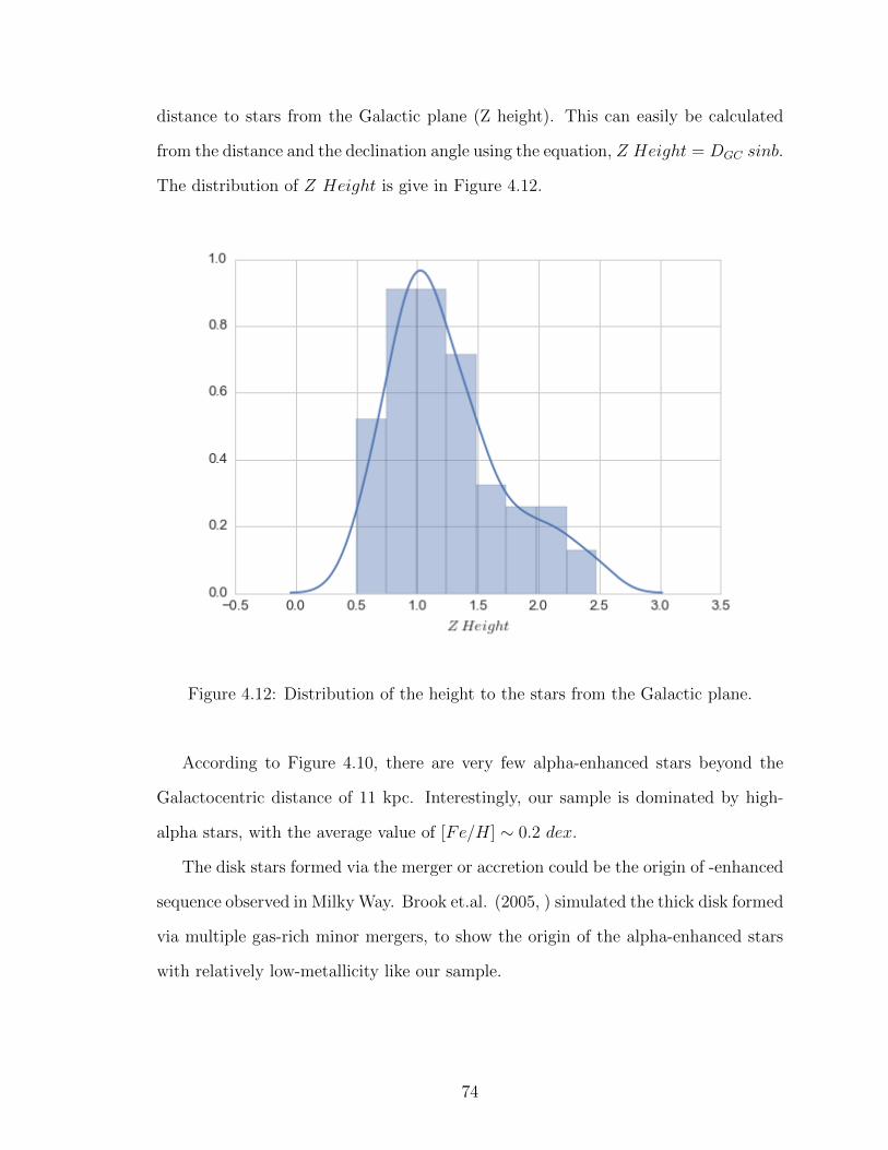
distance to stars from the Galactic plane (Z height). This can easily be calculated
from the distance and the declination angle using the equation, Z Height = DGC sinb.
The distribution of Z Height is give in Figure 4.12.
Figure 4.12: Distribution of the height to the stars from the Galactic plane.
According to Figure 4.10, there are very few alpha-enhanced stars beyond the
Galactocentric distance of 11 kpc. Interestingly, our sample is dominated by high-
alpha stars, with the average value of [Fe/H] ⇠ 0.2 dex.
The disk stars formed via the merger or accretion could be the origin of -enhanced
sequence observed in MilkyWay. Brook et.al. (2005, ) simulated the thick disk formed
via multiple gas-rich minor mergers, to show the origin of the alpha-enhanced stars
with relatively low-metallicity like our sample.
74
4.3 Summary
Using sample of red clump stars, we were able to estimate the chemical and kinemati-
cal charactor of the Canis Major Overdensity. The overall metallicity is in agreement
with expected value for thick disk stars at this distance. The avarage alpha abun-
dance for these stars is ⇠ 0.25 dex. This is in contrast with the few low-alpha stars
observed at Galactocentric distances > 11 kpc of Hayden et.al.
The kinematic distribution of RC stars supports a mixture of thin/thick disk stars,
while the large dispersion of the velocity does not favor a dynamically cold structure.
Few of the concerns we had during this study needs to be mentioned here.
The temperatures of the stars obtained from ULySS are 300 K higher than the
temperatures obtained from The Cannon. This same o↵st was observed between the
temperatures calculated from the spectrum fitting package, SPAce (Stellar Parame-
ters and Chemical abundance Estimator)3 and The Cannon. However, the tempera-
tures obtained from The Cannon are consistant with temperatures predicted by both
stellar isochrones and the APOGEE catalog at this metallicity.
As a test study we estimated E(B�V ) using the stellar parameters adopted from
ULySS. This gave us mean E(B � V ) of 0.3. A separate study conducted by our
group using the Blue Plume stars also predicted E(B�V ) ⇠ 0.3 towards the CMO.
Interestingly, this is in agreement with the Galactic dust maps obtained from Plank
collaboration.
Also, we estimated the [↵/Fe] for our sample using the SPAce. This gave us mean
[↵/Fe] ⇠ 0., which is consistant with the Hayden et.al. (2014). Again, we emphasize
that the [↵/Fe] derived from The Cannon depend on the accuracy of the [↵/Fe]
estimates of the training set and the accuracy of the LAMOST [↵/Fe] values are not
being fully tested yet.
3http://dc.g-vo.org/
75

Chapter 5 Summary and Conclusion
In this work we utilized many di↵erent strategies to determine the stellar parameters
of individual stars. To that end we used all available flux data for a given star. The
main conclusions of the work can be summarised as follows.
5.1 Stellar Parameters in UV
We evaluated the consistency between observed energy distribution of metal-poor
A-type stars and that of Kurucz(ATLAS12) models, especially focusing on the UV
wavelengths. We noticed that the observed and model energy distributions agreed
quite well overall, with slight deviation at far-UV wavelengths. We have estimated
that the model fluxes below 2000 A predict less flux than the observed flux.
5.2 Blue Straggler Stars in the Galactic Field
Combining the flux data from optical and ultraviolet surveys, we were able to adentify
85 hot and young white dwarf companions to field blue straggler stars and measure
their stellar parameters. Based on the WD parameter distribution we conclude that
majority of the WDs are helium WDs formed through case-B mass transfer. Combin-
ing the WD stellar parameters with the evolutionary models we estimated the lower
limit of the binary mass transfer e�ciency in these stars to be, � = 0.5.
5.3 Canis Major Overdensity
The chemical and kinematical charactor of the red clump stars of the Canis Major
Overdensity suggest an in-situ origin of the CMO. The kinematic distribution of
RC stars supports a mixture of thin/thick disk stars, while the large dispersion of
76

the velocity does not favor a dynamically cold structure. The measured interstellar
reddening towards CMO is in agreement with the work of Schlegel et. al (1998).
Copyright c� Gemunu Ekanayake, 2017.
77

Bibliography
[1] Planck Collaboration, R. Adam, P. A. R. Ade, N. Aghanim, Y. Akrami, M. I. R.
Alves, F. Argueso, M. Arnaud, F. Arroja, M. Ashdown, and et al. Planck 2015
results. I. Overview of products and scientific results. A&A, 594:A1, September
2016.
[2] M. Fukugita and P. J. E. Peebles. The Cosmic Energy Inventory. ApJ, 616:643–
668, December 2004.
[3] P. et.al. Andre. From filamentary clouds to prestellar cores to the stellar IMF:
Initial highlights from the Herschel Gould Belt Survey. A&A, 518:L102, July
2010.
[4] F. LeBlanc. An Introduction to Stellar Astrophysics. 2010.
[5] Z. Ivezic, B. Sesar, M. Juric, N. Bond, J. Dalcanton, C. M. Rockosi, B. Yanny,
H. J. Newberg, T. C. Beers, C. Allende Prieto, R. Wilhelm, Y. S. Lee, T. Sivarani,
J. E. Norris, C. A. L. Bailer-Jones, P. Re Fiorentin, D. Schlegel, A. Uomoto,
R. H. Lupton, G. R. Knapp, J. E. Gunn, K. R. Covey, J. Allyn Smith, G. Mik-
naitis, M. Doi, M. Tanaka, M. Fukugita, S. Kent, D. Finkbeiner, J. A. Munn,
J. R. Pier, T. Quinn, S. Hawley, S. Anderson, F. Kiuchi, A. Chen, J. Bushong,
H. Sohi, D. Haggard, A. Kimball, J. Barentine, H. Brewington, M. Harvanek,
S. Kleinman, J. Krzesinski, D. Long, A. Nitta, S. Snedden, B. Lee, H. Harris,
J. Brinkmann, D. P. Schneider, and D. G. York. The Milky Way Tomography
with SDSS. II. Stellar Metallicity. ApJ, 684:287–325, September 2008.
[6] J. Debosscher, L. M. Sarro, C. Aerts, J. Cuypers, B. Vandenbussche, R. Garrido,
78

and E. Solano. VizieR Online Data Catalog: Supervised classification of variable
stars (Debosscher+, 2007). VizieR Online Data Catalog, 347, November 2007.
[7] P. Dubath, L. Rimoldini, M. Suveges, J. Blomme, M. Lopez, L. M. Sarro, J. De
Ridder, J. Cuypers, L. Guy, I. Lecoeur, K. Nienartowicz, A. Jan, M. Beck,
N. Mowlavi, P. De Cat, T. Lebzelter, and L. Eyer. Random forest automated
supervised classification of Hipparcos periodic variable stars. MNRAS, 414:2602–
2617, July 2011.
[8] D. N. C. Lin and S. M. Faber. Some implications of nonluminous matter in
dwarf spheroidal galaxies. ApJ, 266:L21–L25, March 1983.
[9] F. Beutler, C. Blake, M. Colless, D. H. Jones, L. Staveley-Smith, L. Campbell,
Q. Parker, W. Saunders, and F. Watson. The 6dF Galaxy Survey: baryon
acoustic oscillations and the local Hubble constant. MNRAS, 416:3017–3032,
October 2011.
[10] M. Montes, J. A. Acosta-Pulido, M. A. Prieto, and J. A. Fernandez-Ontiveros.
The innermost globular clusters of M87. MNRAS, 442:1350–1362, August 2014.
[11] F. Hernandez-Perez and G. Bruzual. Binary stars and the UVX in early-type
galaxies. MNRAS, 444:2571–2579, November 2014.
[12] S. Kaviraj, K. Schawinski, J. E. G. Devriendt, I. Ferreras, S. Khochfar, S.-J.
Yoon, S. K. Yi, J.-M. Deharveng, A. Boselli, T. Barlow, T. Conrow, K. Forster,
P. G. Friedman, D. C. Martin, P. Morrissey, S. Ne↵, D. Schiminovich, M. Seibert,
T. Small, T. Wyder, L. Bianchi, J. Donas, T. Heckman, Y.-W. Lee, B. Madore,
B. Milliard, R. M. Rich, and A. Szalay. UV-Optical Colors As Probes of Early-
Type Galaxy Evolution. ApJS, 173:619–642, December 2007.
79

[13] H.-c. Lee, Y.-W. Lee, and B. K. Gibson. Horizontal-Branch Morphology and the
Photometric Evolution of Old Stellar Populations. AJ, 124:2664–2676, November
2002.
[14] C. Maraston and D. Thomas. Strong Balmer Lines in Old Stellar Populations:
No Need for Young Ages in Ellipticals? ApJ, 541:126–133, September 2000.
[15] J. A. Rose. Spectral anomalies in the Hyades and Pleiades and in field stars with
active chromospheres. AJ, 89:1238–1251, August 1984.
[16] D. P. Huenemoerder and S. C. Barden. Spectroscopy of RS CVn and W UMa
Systems: Extraction of Component Spectra. In Bulletin of the American Astro-
nomical Society, volume 16 of BAAS, page 510, March 1984.
[17] M. N. Fanelli, R. W. O’Connell, D. Burstein, and C.-C. Wu. Spectral synthesis
in the ultraviolet. IV - A library of mean stellar groups. ApJS, 82:197–245,
September 1992.
[18] A. Heck, D. Egret, M. Jaschek, and C. Jaschek. IUE low-dispersion spectra flux
catalogue. I - Normal stars (magnetic tape). A&AS, 57:213–216, August 1984.
[19] M. D. Gregg, D. Silva, J. Rayner, F. Valdes, G. Worthey, A. Pickles, J. A. Rose,
W. Vacca, and B. Carney. The HST/STIS Next Generation Spectral Library.
In American Astronomical Society Meeting Abstracts, volume 36 of Bulletin of
the American Astronomical Society, page 1496, December 2004.
[20] J. A. Cardelli, G. C. Clayton, and J. S. Mathis. The relationship between in-
frared, optical, and ultraviolet extinction. ApJ, 345:245–256, October 1989.
[21] R. O. Gray and C. J. Corbally. The calibration of MK spectral classes using
spectral synthesis. 1: The e↵ective temperature calibration of dwarf stars. AJ,
107:742–746, February 1994.
80
[22] A. R. Sandage. The color-magnitude diagram for the globular cluster M 3. AJ,
58:61–75, 1953.
[23] R. D. Mathieu and A. M. Geller. A binary star fraction of 76 per cent and
unusual orbit parameters for the blue stragglers of NGC 188. Nature, 462:1032–
1035, December 2009.
[24] F. R. Ferraro, B. Paltrinieri, R. T. Rood, and B. Dorman. Blue Straggler Stars:
The Spectacular Population in M80. ApJ, 522:983–990, September 1999.
[25] Y. Momany, E. V. Held, I. Saviane, S. Zaggia, L. Rizzi, and M. Gullieuszik. The
blue plume population in dwarf spheroidal galaxies. Genuine blue stragglers or
young stellar population? A&A, 468:973–978, June 2007.
[26] G. W. Preston and C. Sneden. What Are These Blue Metal-Poor Stars? AJ,
120:1014–1055, August 2000.
[27] L. Deng, R. Chen, X. S. Liu, and J. S. Chen. The Blue Stragglers in M67 and
Single-Population Synthesis. ApJ, 524:824–830, October 1999.
[28] J. C. Wheeler. Blue stragglers as long-lived stars. ApJ, 234:569–578, December
1979.
[29] W. H. McCrea. Extended main-sequence of some stellar clusters. MNRAS,
128:147, 1964.
[30] R. Kippenhahn and A. Weigert. Entwicklung in engen Doppelsternsystemen I.
Massenaustausch vor und nach Beendigung des zentralen Wassersto↵-Brennens.
ZAp, 65:251, 1967.
[31] X. Chen and Z. Han. Primordial binary evolution and blue stragglers. MNRAS,
395:1822–1836, June 2009.
81
[32] S. G. Ryan, S. G. Gregory, U. Kolb, T. C. Beers, and T. Kajino. Rapid Rotation
of Ultra-Li-depleted Halo Stars and Their Association with Blue Stragglers. ApJ,
571:501–511, May 2002.
[33] G. W. Preston and A. U. Landolt. Pulsating Blue Metal-poor Stars. AJ,
118:3006–3015, December 1999.
[34] B. Yanny, H. J. Newberg, S. Kent, S. A. Laurent-Muehleisen, J. R. Pier, G. T.
Richards, C. Stoughton, J. E. Anderson, Jr., J. Annis, J. Brinkmann, B. Chen,
I. Csabai, M. Doi, M. Fukugita, G. S. Hennessy, Z. Ivezic, G. R. Knapp, R. Lup-
ton, J. A. Munn, T. Nash, C. M. Rockosi, D. P. Schneider, J. A. Smith, and D. G.
York. Identification of A-colored Stars and Structure in the Halo of the Milky
Way from Sloan Digital Sky Survey Commissioning Data. ApJ, 540:825–841,
September 2000.
[35] E. Sirko, J. Goodman, G. R. Knapp, J. Brinkmann, Z. Ivezic, E. J. Knerr,
D. Schlegel, D. P. Schneider, and D. G. York. Blue Horizontal-Branch Stars in
the Sloan Digital Sky Survey. II. Kinematics of the Galactic Halo. AJ, 127:914–
924, February 2004.
[36] X. X. Xue, H. W. Rix, G. Zhao, P. Re Fiorentin, T. Naab, M. Steinmetz, F. C.
van den Bosch, T. C. Beers, Y. S. Lee, E. F. Bell, C. Rockosi, B. Yanny, H. New-
berg, R. Wilhelm, X. Kang, M. C. Smith, and D. P. Schneider. The Milky Way’s
Circular Velocity Curve to 60 kpc and an Estimate of the Dark Matter Halo
Mass from the Kinematics of ˜2400 SDSS Blue Horizontal-Branch Stars. ApJ,
684:1143–1158, September 2008.
[37] Y. S. Lee, T. C. Beers, T. Sivarani, C. Allende Prieto, L. Koesterke, R. Wilhelm,
P. Re Fiorentin, C. A. L. Bailer-Jones, J. E. Norris, C. M. Rockosi, B. Yanny,
H. J. Newberg, K. R. Covey, H.-T. Zhang, and A.-L. Luo. The SEGUE Stellar
82

Parameter Pipeline. I. Description and Comparison of Individual Methods. AJ,
136:2022–2049, November 2008.
[38] Tamas Budavari et.al. Galex-sdss catalogs for statistical studies. The Astrophys-
ical Journal, 694(2):1281, 2009.
[39] E. F. Schlafly and D. P. Finkbeiner. Measuring Reddening with Sloan Digital
Sky Survey Stellar Spectra and Recalibrating SFD. ApJ, 737:103, August 2011.
[40] S.-C. Rey, R. M. Rich, S. T. Sohn, S.-J. Yoon, C. Chung, S. K. Yi, Y.-W. Lee,
J. Rhee, L. Bianchi, B. F. Madore, K. Lee, T. A. Barlow, K. Forster, P. G.
Friedman, D. C. Martin, P. Morrissey, S. G. Ne↵, D. Schiminovich, M. Seibert,
T. Small, T. K. Wyder, J. Donas, T. M. Heckman, B. Milliard, A. S. Szalay,
and B. Y. Welsh. GALEX Ultraviolet Photometry of Globular Clusters in M31:
Three-Year Results and a Catalog. ApJS, 173:643–658, December 2007.
[41] D. J. Schlegel, D. P. Finkbeiner, and M. Davis. Maps of Dust Infrared Emis-
sion for Use in Estimation of Reddening and Cosmic Microwave Background
Radiation Foregrounds. ApJ, 500:525–553, June 1998.
[42] A. Rebassa-Mansergas, A. Nebot Gomez-Moran, M. R. Schreiber, B. T.
Gansicke, A. Schwope, J. Gallardo, and D. Koester. Post-common envelope bi-
naries from SDSS - XIV. The DR7 white dwarf-main-sequence binary catalogue.
MNRAS, 419:806–816, January 2012.
[43] M. A. Smith, L. Bianchi, and B. Shiao. Interesting Features in the Combined
GALEX and Sloan Color Diagrams of Solar-like Galactic Populations. AJ,
147:159, June 2014.
[44] M. A. Wood. Theoretical White Dwarf Luminosity Functions: DA Models. In
D. Koester and K. Werner, editors, White Dwarfs, volume 443 of Lecture Notes
in Physics, Berlin Springer Verlag, page 41, 1995.
83

[45] G. Fontaine, P. Brassard, and P. Bergeron. The Potential of White Dwarf Cos-
mochronology. PASP, 113:409–435, April 2001.
[46] M. Fukugita, T. Ichikawa, J. E. Gunn, M. Doi, K. Shimasaku, and D. P. Schnei-
der. The Sloan Digital Sky Survey Photometric System. AJ, 111:1748, April
1996.
[47] C. Zhao and H. J. Newberg. Transformation from SDSS Photometric System
to Johnson-Morgan-Cousins System in HK Survey. ArXiv Astrophysics e-prints,
December 2006.
[48] T. C. Beers, D. Carollo, Z. Ivezic, D. An, M. Chiba, J. E. Norris, K. C. Freeman,
Y. S. Lee, J. A. Munn, P. Re Fiorentin, T. Sivarani, R. Wilhelm, B. Yanny,
and D. G. York. The Case for the Dual Halo of the Milky Way. ApJ, 746:34,
February 2012.
[49] T. D. Kinman, N. B. Suntze↵, and R. P. Kraft. The structure of the galactic
halo outside the solar circle as traced by the blue horizontal branch stars. AJ,
108:1722–1772, November 1994.
[50] G. Torres. On the Use of Empirical Bolometric Corrections for Stars. AJ,
140:1158–1162, November 2010.
[51] J. R. Hurley, C. A. Tout, and O. R. Pols. Evolution of binary stars and the
e↵ect of tides on binary populations. MNRAS, 329:897–928, February 2002.
[52] Donald Knuth. Knuth: Computers and typesetting.
[53] Y. Momany, S. R. Zaggia, P. Bonifacio, G. Piotto, F. De Angeli, L. R. Bedin,
and G. Carraro. Probing the Canis Major stellar over-density as due to the
Galactic warp. A&A, 421:L29–L32, July 2004.
84

[54] J. P. De Greve and C. De Loore. Evolution of massive close binaries. A&AS,
96:653–663, December 1992.
[55] X. Chen and Z. Han. Primordial binary evolution and blue stragglers. MNRAS,
395:1822–1836, June 2009.
[56] A. Pietrinferni, S. Cassisi, M. Salaris, and F. Castelli. A Large Stellar Evolution
Database for Population Synthesis Studies. II. Stellar Models and Isochrones for
an ↵-enhanced Metal Distribution. ApJ, 642:797–812, May 2006.
[57] P. Jofre and A. Weiss. The age of the Milky Way halo stars from the Sloan
Digital Sky Survey. A&A, 533:A59, September 2011.
[58] N. F. Martin, R. A. Ibata, M. Bellazzini, M. J. Irwin, G. F. Lewis, and
W. Dehnen. A dwarf galaxy remnant in Canis Major: the fossil of an in-plane
accretion on to the Milky Way. MNRAS, 348:12–23, February 2004.
[59] H. J. Newberg, B. Yanny, C. Rockosi, E. K. Grebel, H.-W. Rix, J. Brinkmann,
I. Csabai, G. Hennessy, R. B. Hindsley, R. Ibata, Z. Ivezic, D. Lamb, E. T. Nash,
M. Odenkirchen, H. A. Rave, D. P. Schneider, J. A. Smith, A. Stolte, and D. G.
York. The Ghost of Sagittarius and Lumps in the Halo of the Milky Way. ApJ,
569:245–274, April 2002.
[60] J. Penarrubia and A. J. Benson. E↵ects of dynamical evolution on the distribu-
tion of substructures. MNRAS, 364:977–989, December 2005.
[61] Y. Momany, S. R. Zaggia, P. Bonifacio, G. Piotto, F. De Angeli, L. R. Bedin,
and G. Carraro. Probing the Canis Major stellar over-density as due to the
Galactic warp. A&A, 421:L29–L32, July 2004.
[62] D. J. Schlegel, D. P. Finkbeiner, and M. Davis. Maps of Dust Infrared Emis-
sion for Use in Estimation of Reddening and Cosmic Microwave Background
Radiation Foregrounds. ApJ, 500:525–553, June 1998.
85
[63] P. Bonifacio, V. Hill, P. Molaro, L. Pasquini, P. Di Marcantonio, and P. Santin.
First results of UVES at VLT: abundances in the Sgr dSph. A&A, 359:663–668,
July 2000.
[64] D. Hatzidimitriou and M. R. S. Hawkins. Stellar populations and large-scale
structure of the SMC. II - Geometry of the north-eastern and south-western
outlying regions. MNRAS, 241:667–690, December 1989.
[65] L. Girardi and M. Salaris. Population e↵ects on the red giant clump absolute
magnitude, and distance determinations to nearby galaxies. MNRAS, 323:109–
129, May 2001.
[66] K. Z. Stanek and P. M. Garnavich. Red Clump Stars - New, Improved Distance
Indicator. In American Astronomical Society Meeting Abstracts, volume 30 of
Bulletin of the American Astronomical Society, page 1409, December 1998.
[67] K. C. Chambers, E. A. Magnier, N. Metcalfe, H. A. Flewelling, M. E. Huber,
C. Z. Waters, L. Denneau, P. W. Draper, D. Farrow, D. P. Finkbeiner, C. Holm-
berg, J. Koppenhoefer, P. A. Price, R. P. Saglia, E. F. Schlafly, S. J. Smartt,
W. Sweeney, R. J. Wainscoat, W. S. Burgett, T. Grav, J. N. Heasley, K. W.
Hodapp, R. Jedicke, N. Kaiser, R.-P. Kudritzki, G. A. Luppino, R. H. Lupton,
D. G. Monet, J. S. Morgan, P. M. Onaka, C. W. Stubbs, J. L. Tonry, E. Ba-
nados, E. F. Bell, R. Bender, E. J. Bernard, M. T. Botticella, S. Casertano,
S. Chastel, W.-P. Chen, X. Chen, S. Cole, N. Deacon, C. Frenk, A. Fitzsim-
mons, S. Gezari, C. Goessl, T. Goggia, B. Goldman, E. K. Grebel, N. C. Ham-
bly, G. Hasinger, A. F. Heavens, T. M. Heckman, R. Henderson, T. Henning,
M. Holman, U. Hopp, W.-H. Ip, S. Isani, C. D. Keyes, A. Koekemoer, R. Ko-
tak, K. S. Long, J. R Lucey, M. Liu, N. F. Martin, B. McLean, E. Morganson,
D. N. A. Murphy, M. A. Nieto-Santisteban, P. Norberg, J. A. Peacock, E. A.
Pier, M. Postman, N. Primak, C. Rae, A. Rest, A. Riess, A. Ri↵eser, H. W. Rix,
86

S. Roser, E. Schilbach, A. S. B. Schultz, D. Scolnic, A. Szalay, S. Seitz, B. Shiao,
E. Small, K. W. Smith, D. Soderblom, A. N. Taylor, A. R. Thakar, J. Thiel,
D. Thilker, Y. Urata, J. Valenti, F. Walter, S. P. Watters, S. Werner, R. White,
W. M. Wood-Vasey, and R. Wyse. The Pan-STARRS1 Surveys. ArXiv e-prints,
December 2016.
[68] J. Bovy, D. L. Nidever, H.-W. Rix, L. Girardi, G. Zasowski, S. D. Chojnowski,
J. Holtzman, C. Epstein, P. M. Frinchaboy, M. R. Hayden, T. S. Rodrigues,
S. R. Majewski, J. A. Johnson, M. H. Pinsonneault, D. Stello, C. Allende Pri-
eto, B. Andrews, S. Basu, T. C. Beers, D. Bizyaev, A. Burton, W. J. Chaplin,
K. Cunha, Y. Elsworth, R. A. Garcıa, D. A. Garcıa-Hernandez, A. E. Garcıa
Perez, F. R. Hearty, S. Hekker, T. Kallinger, K. Kinemuchi, L. Koesterke,
S. Meszaros, B. Mosser, R. W. O’Connell, D. Oravetz, K. Pan, A. C. Robin,
R. P. Schiavon, D. P. Schneider, M. Schultheis, A. Serenelli, M. Shetrone, V. Silva
Aguirre, A. Simmons, M. Skrutskie, V. V. Smith, K. Stassun, D. H. Weinberg,
J. C. Wilson, and O. Zamora. The APOGEE Red-clump Catalog: Precise Dis-
tances, Velocities, and High-resolution Elemental Abundances over a Large Area
of the Milky Way’s Disk. ApJ, 790:127, August 2014.
[69] A. Y. Q. Ho, M. K. Ness, D. W. Hogg, H.-W. Rix, C. Liu, F. Yang, Y. Zhang,
Y. Hou, and Y. Wang. Label Transfer from APOGEE to LAMOST: Precise
Stellar Parameters for 450,000 LAMOST Giants. ApJ, 836:5, February 2017.
[70] M. Koleva, P. Prugniel, A. Bouchard, and Y. Wu. ULySS: a full spectrum fitting
package. A&A, 501:1269–1279, July 2009.
[71] M. Ness, D. W. Hogg, H.-W. Rix, A. Y. Q. Ho, and G. Zasowski. The Cannon:
A data-driven approach to Stellar Label Determination. ApJ, 808:16, July 2015.
[72] X.-Q. Cui, Y.-H. Zhao, Y.-Q. Chu, G.-P. Li, Q. Li, L.-P. Zhang, H.-J. Su, Z.-Q.
87

Yao, Y.-N. Wang, X.-Z. Xing, X.-N. Li, Y.-T. Zhu, G. Wang, B.-Z. Gu, A.-L.
Luo, X.-Q. Xu, Z.-C. Zhang, G.-R. Liu, H.-T. Zhang, D.-H. Yang, S.-Y. Cao,
H.-Y. Chen, J.-J. Chen, K.-X. Chen, Y. Chen, J.-R. Chu, L. Feng, X.-F. Gong,
Y.-H. Hou, H.-Z. Hu, N.-S. Hu, Z.-W. Hu, L. Jia, F.-H. Jiang, X. Jiang, Z.-B.
Jiang, G. Jin, A.-H. Li, Y. Li, Y.-P. Li, G.-Q. Liu, Z.-G. Liu, W.-Z. Lu, Y.-
D. Mao, L. Men, Y.-J. Qi, Z.-X. Qi, H.-M. Shi, Z.-H. Tang, Q.-S. Tao, D.-Q.
Wang, D. Wang, G.-M. Wang, H. Wang, J.-N. Wang, J. Wang, J.-L. Wang, J.-P.
Wang, L. Wang, S.-Q. Wang, Y. Wang, Y.-F. Wang, L.-Z. Xu, Y. Xu, S.-H.
Yang, Y. Yu, H. Yuan, X.-Y. Yuan, C. Zhai, J. Zhang, Y.-X. Zhang, Y. Zhang,
M. Zhao, F. Zhou, G.-H. Zhou, J. Zhu, and S.-C. Zou. The Large Sky Area Multi-
Object Fiber Spectroscopic Telescope (LAMOST). Research in Astronomy and
Astrophysics, 12:1197–1242, September 2012.
[73] M. S. Bessell. UBVRI passbands. PASP, 102:1181–1199, October 1990.
[74] J. L. Tonry, C. W. Stubbs, K. R. Lykke, P. Doherty, I. S. Shivvers, W. S.
Burgett, K. C. Chambers, K. W. Hodapp, N. Kaiser, R.-P. Kudritzki, E. A.
Magnier, J. S. Morgan, P. A. Price, and R. J. Wainscoat. The Pan-STARRS1
Photometric System. ApJ, 750:99, May 2012.
[75] K. Z. Stanek and P. M. Garnavich. Distance to M31 with the Hubble Space
Telescope and HIPPARCOS Red Clump Stars. ApJ, 503:L131–L134, August
1998.
[76] M. Valentini and U. Munari. A spectroscopic survey of faint, high-Galactic-
latitude red clump stars. I. The high resolution sample. A&A, 522:A79, Novem-
ber 2010.
[77] D. R. Alves. K-Band Calibration of the Red Clump Luminosity. ApJ, 539:732–
741, August 2000.
88

[78] V. van Helshoecht and M. A. T. Groenewegen. K-band magnitude of the red
clump as a distance indicator. A&A, 463:559–565, February 2007.
[79] L.-C. Deng, H. J. Newberg, C. Liu, J. L. Carlin, T. C. Beers, L. Chen, Y.-Q.
Chen, N. Christlieb, C. J. Grillmair, P. Guhathakurta, Z.-W. Han, J.-L. Hou,
H.-T. Lee, S. Lepine, J. Li, X.-W. Liu, K.-K. Pan, J. A. Sellwood, B. Wang, H.-
C. Wang, F. Yang, B. Yanny, H.-T. Zhang, Y.-Y. Zhang, Z. Zheng, and Z. Zhu.
LAMOST Experiment for Galactic Understanding and Exploration (LEGUE)
The survey’s science plan. Research in Astronomy and Astrophysics, 12:735–
754, July 2012.
[80] W. Dehnen and J. J. Binney. Local stellar kinematics from HIPPARCOS data.
MNRAS, 298:387–394, August 1998.
[81] A. Boehle, A. M. Ghez, R. Schodel, L. Meyer, S. Yelda, S. Albers, G. D. Martinez,
E. E. Becklin, T. Do, J. R. Lu, K. Matthews, M. R. Morris, B. Sitarski, and
G. Witzel. An Improved Distance and Mass Estimate for Sgr A* from a Multistar
Orbit Analysis. ApJ, 830:17, October 2016.
[82] W. D. Arnett. On the bulk yields of nucleosynthesis from massive stars. ApJ,
219:1008–1016, February 1978.
[83] M. R. Hayden, J. A. Holtzman, J. Bovy, S. R. Majewski, J. A. Johnson, C. Al-
lende Prieto, T. C. Beers, K. Cunha, P. M. Frinchaboy, A. E. Garcıa Perez, L. Gi-
rardi, F. R. Hearty, Y. S. Lee, D. Nidever, R. P. Schiavon, K. J. Schlesinger, D. P.
Schneider, M. Schultheis, M. Shetrone, V. V. Smith, G. Zasowski, D. Bizyaev,
D. Feuillet, S. Hasselquist, K. Kinemuchi, E. Malanushenko, V. Malanushenko,
R. O’Connell, K. Pan, and K. Stassun. Chemical Cartography with APOGEE:
Large-scale Mean Metallicity Maps of the Milky Way Disk. AJ, 147:116, May
2014.
89

Vita
Gemunu Ekanayake
Education
Ph.D. Physics ......................................................................... expected May 2017
University of Kentucky, Lexington, Kentucky, United States
M.Sc. Physics ......................................................................... May 2014
University of Kentucky, Lexington, Kentucky, United States
B.S. Physics ......................................................................... August 2008
University of Peradeniya, Kandy, Sri Lanka
Professional Positions Held
Graduate Assistant ................................................................... Sept 2015 - present
University of Kentucky, Lexington, Kentucky, United States
Teaching Assistant ................................................................... Sept 2009 - May 2013
University of Kentucky, Lexington, Kentucky, United States
Society Memberships
American Physical Society
American Astronomical Society
90