Embed Size (px)
Citation preview

Rochester Institute of Technology Rochester Institute of Technology
RIT Scholar Works RIT Scholar Works
Theses
1991
Determination of the thermal properties of thin polymer films Determination of the thermal properties of thin polymer films
Duane A. Swanson
Follow this and additional works at: https://scholarworks.rit.edu/theses
Recommended Citation Recommended Citation Swanson, Duane A., "Determination of the thermal properties of thin polymer films" (1991). Thesis. Rochester Institute of Technology. Accessed from
This Thesis is brought to you for free and open access by RIT Scholar Works. It has been accepted for inclusion in Theses by an authorized administrator of RIT Scholar Works. For more information, please contact [email protected].

DETERMINATION OF THE THERMAL PROPERTIESOF THIN POLYMER FILMS
byDuane A. Swanson
A Thesis Submittedin
Partial Fulfillmentof the
Requirements for the Degree ofMASTER OF SCIENCE
in Mechanical Engineeringat
Rochester Institute of Technology
Approved by:
Dr. Joseph S. Torok, Thesis Co-AdvisorMechanical Engineering DepartmentRochester Institute of Technology
Dr. Ali Ogut, Thesis Co-AdvisorMechanical Engineering DepartmentRochester Institute of Technology
Dr. Alan NyeMechanical Engineering DepartmentRochester Institute of Technology
Mr. Richard CianciottoManager of Process Technology DepartmentMobil Chemical Company, Films Division
Dr. Charles Haines, Department HeadMechanical Engineering DepartmentRochester Institute of Technology

I, Duane A. Swanson, do hereby grant permission to
Wallace Memorial Library, of R.I.T., to reproduce my
thesis in whole or part. Any reproduction will not be
used for commercial use or profit.

ACKNOWLEDGEMENT
To Mobil Chemical Company, Films Division, especially Richard
Cianciotto and Sharon Kemp-Patchett,
for their support and
initiating this research work with R.I.T., I express sincere
gratitude.
To R.I.T. Mechanical Engineering Faculty Members, who have
instilled me with vast knowledge and experience throughout my
college career, many thanks.
To Dr. Joseph S. Torok, my professor, advisor, mentor, and friend,
I express deepest gratitude and appreciation.
To my Mother and Father, my appreciation for providing support and
encouragement to allow me to achieve.
Most of all, I would like to thank my wife, Nancy. For her
patience, understanding, and love, I dedicate this work.
ABSTRACT
The purpose of this investigation was to analyze heat transfer
characteristics of cavitated-core polymer films. The effects of
thickness and composition on the insulative properties of thin
polymer films were studied.
Two experimental tests were developed to measure the heat
transfer rate through a variety of thin films. One test apparatus
was used to study convective and radiative effects while the second
was used to study the conductive effects.
A finite element model of a frozen food commodity wrapped in
an insulative thin film was developed. Transient simulations were
performed for the dynamic characterization of thermal wave
propagation across the film layer. This model was then used to
compare insulative properties associated with various packaging
films .
Experiments established that radiation effects are very
significant in the freezer environment. Experiments also verified
that cavitated-core films were more insulative than solid films.
Modeling results illustrated that thickness and conductivity of a
thin film only have insulative significance when exposed to a
purely conductive environment.

TABLE OF CONTENTS
ABSTRACT i
1.0 Introduction 1
2.0 Theory & Literature Review 3
2.1 Heat Transfer Theory 3
2.2 Heat Transfer Methods for Thin Films 10
3.0 Materials & Methods 13
3.1 Apparatus & Procedures 13
3.1.1 Insulated Box 13
3.1.2 Thermal Analyzer 15
4.0 Results and Discussion 17
4.1 Insulated Box -
Emissivity Factor 17
4.2 Thermal Analyzer - Transient Conduction Response 25
4.3 Statistical Analysis 33
5.0 Modeling and Simulation 39
5.1 Insulated Box - Verification of Test Results 39
5.2 Finite Element Modeling Theory 46
5.3 Thermal Analyzer - Pure Conduction 54
5.3.1 Galerkin Approximation 54
5.3.2 Determination of Apparent Conductivities 64
5.4 Freezer Environment 66
5.4.1 Response Characteristics
5.4.2 Dynamic Formulation
5.4.3 Summary of Freezer Simulation results
6.0 Conclusions & Recommendations
7.0 References
8.0 Appendix
8.1 Fortran List Files
8 . 2 Additional Responses
n
66
70
74
84
87
88
89
102

TABLES
4.1 The Relationship Between Gauge and Kapp for 26
a particular film type.
5.1 Material List With Apparent Conductivity 65
5.2 Conduction : Summary of Freezer Simulation 81
Nodal Temperatures
5.3 Convection : Summary of Freezer Simulation 82
Nodal Temperatures
5.4 Convection & Radiation : Summary of Freezer 83
Simulation Nodal Temperatures
m

FIGURES
1
2
,3
,4
.5
,6
,7
3.1
3.2
4.1
Modes of Heat Transfer
Differential Control Volume, dxdydz
Conduction
Convection
Thermal Radiation
Net Radiation
Hot/Cold Temperature Differential
Insulated Box
Thermal Analyzer
Freeze cycles of 1.0 mil coex/1.0 mil coex OPP,1.0 mil coex OPP, 1.1 mil coated OPPalyte/.75 mil
cellophane.
4.2 Freeze cycles of aluminum foil, white pigmented
polyethylene, 1.5 mil uncoated OPPalyte, and
metallized 1.50 mil uncoated OPPalyte.
4.3 Freeze cycles of aluminum foil, 1.4 mil metallyte,
wax paper, and 1.4 mil uncoated OPPalyte.
4.4 Freeze cycles with Insulated Box filled with
antifreeze and air. 1.5 mil poylethelyne vs.
.72 mil aluminum foil.
4.5 Thermal Analyzer results showing metallized vs.
OPPalytes and non-OPPalytes.
4.6 Thermal Analyzer results showing the effect of gauge
for uncoated OPPalytes.
4.7 Thermal Analyzer Results showing the effect of gauge
for oriented polypropylene.
4.8 Thermal Analyzer results showing OPPalytes vs.
non-OPPalytes .
4.9 Thermal Analyzer results showing metallized vs.
1.50 mil uncoated OPPalyte.
4.10 95% Confidence Interval Bars on Insulated Box Results
4.11 Thermal Analyzer Results of 1.40 Metallyte with
95% Confidence Interval Bars
4.12 Thermal Analyzer Results of 1.40 mil Coextruded
Oriented Polypropylene w/ 95% Confidence Int. Bars
4.13 Thermal Analyzer Results of 1.50 mil coated OPPalyte
w/ 95% Confidence Interval Bars
4.14 Thermal Analyzer Results of 1.77 mil High OpacityWhite w/ 95% Confidence Interval Bars
3
4
6
8
8
9
12
14
15
19
20
21
22
27
28
29
31
32
34
35
36
37
38
IV
FIGURES
5.1 Insulated Box Schematic 39
5.2A Theoretical freeze cycle with and without antifreeze. 43
5.2B Theoretical freeze cycle with effect of film 44
emissitivity.
5.2C Percent of Heat Flux due to Radiative Effects 45
5.3 Thermal Analyzer 1-D Schematic 54
5.4 Temperature distribution in the domains. 55
5.5 System response for selected values of k,. 64
5.6 Various input temperature profiles. 69
5.7 Package elements 70
5.8 Pure Conduction : Dynamic response of nodal 78
temperatures .
5.9 Pure Convection : Dynamic response of nodal 79
temperatures .
5.10 Convection and Radiation : Dynamic response of 80
nodal temperatures.
8.1 Thermal Analyzer response of laminated substrates103
8.2 Thermal Analyzer response 104
8.3 Thermal Analyzer response 105
8 . 4 Thermal Analyzer response 106

Nomenc1ature
As surface area,m2
Cp specific heat, J/kgK
D depth, m
Eq rate of energy generation, W
Eln rate of energy transfer into a control volume, W
Eout rate of energy transfer out of a control volume, W
Est rate of increase in internal stored energy, W
h convection heat transfer coefficient, W/m2K
h average convection heat transfer coef.,W/m2K
k thermal conductivity, W/mK
L length, m
q heat transfer rate, W
q" heat flux,W/m2
T temperature ,K
t time,s
V Volume ,
m3
Greek Letters
a thermal diffusivity, m2/s
r boundary conditions
e emissitivity ,m2/s
a Stefan-Boltzman constant (5.67E-08 W/m2K4)
p mass density,kg/m3
* appropriate functions
n domain
VI

DETERMINATION OF THE THERMAL PROPERTIES OF POLYMER THIN FILMS
Program : FreezelO : ACSL : RIT VAX/VMS
Programmer : Duane A. Swanson
Abstract : The ACSL program solves a system of ten differential
equations that represent a Finite Element Model designed to
estimate the transient heat transfer of a frozen commodity
wrapped in an insulating film and subjected to various inputs. "
PROGRAM FREEZE10
DERIVATIVE
CONSTANT TSTP = 1200.,...
T20 =-1. , . . .
(WiflD
T60 =-1. ,
T10O= -1.,
. . .
T30 =-1. ,
T70 = -1. ,T110
T40 = -1.,
T80 = -1.,. . .
T50 = -1. , T90 = -1.,.
HE =
.015,. . .
DELTAX = 2.45E-05,...
PI = 3.14159, . . .
ALPHA = 3.09E-07, . . .
KF =
.10,. . .
TAVE = -1 .,
. . .
TAMP = 5 . ,. . .
KAIR = 24.3E-03, . . .
HAIR = 2.5,...
ill = J-f
* *
A #/
RHOC = 3.33E6
C INTERVAL CINT = 1.
ii
=
-1.01,
CI = ALPHA/ (HE)
C2 = 6./(HE*100. )
MT = T/60
'"Vario environmental inputs the model can be subjected to.
"CASE 1 HARMONICINPUT"
"TINF = TAVE + TAMP*SIN(T*3.14159/600)"
"CASE 2 TINF STEP INPUT"
"Y = PULSE(0. ,1200. ,200.)"
X = PULSE( 200. ,2400. ,800.)"
HZ = PULSE(1000. ,3600. ,400. )"
"TINF= TAVE + (1.5)*Y*MT + X*TAMP -
( . 75 ) *Z* (MT-10 . )
96

1.0 INTRODUCTION
Polymer plastic films are widely used in packaging of food
commodities. These films are becoming ever more popular, due to
ease of manufacturing and printability ,for prolonging product
shelf-life. Many of the films used in the packaging of freezer and
refrigerator commodities consist of a solid polymer. A new
packaging substrate has been developed consisting of several layers
in which a cavitated core is sandwiched between two solid film
layers. This composite structure manufactured by a cavitating
process is hypothesized to provide better thermal protection.
This approach is different compared to past packaging film
development in that thermal protection is included in the design of
the composite layers. Most of the previous design considerations
have focused on tensile and puncture strength, printability, and
water vapor transmission properties.
The objective of this work was to carry out an experimental
and theoretical study to investigate the thermal characteristics of
composite films such as cavitated 0PPalyte(TM), white polyethylene,
clear coextruded polypropylene, and metallized films in comparison
to other conventional packaging materials. The thermal response to
all three modes of heat transfer, i.e. convection, conduction, and
radiation, will be considered.
Using the Finite Element Method, the mechanism of heat
transfer through a film is mathematically modeled. With this model,
1

the experimental setup will be verified by establishing a high
level of confidence. Further, apparent conductivities will be found
for typical composite films. Once these thermal parameters are set,
one can use a model that simulates a frozen commodity wrapped in an
insulative film subject to various freezer environments ( i.e.
freezer cycling or temperature shock) . This modelling allows for
comparison of different films (solid, cavitated, metallized, etc..)
with respect to their insulative properties and effectiveness in
storing frozen commodities.

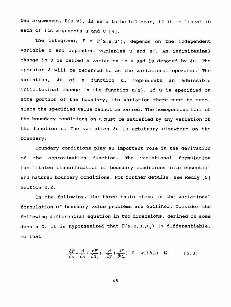
2.0 Theory and Literature Review:
2.1 Heat Transfer Theory :
Heat is transported through a medium (gas, liquid, or solid)
due to a temperature difference at two different points. Heat flows
from a high temperature region to a low temperature region.
Temperature is fundamentally a potential field denoting the
relative energy of the substance [1J. This transmission of energy
takes place in three modes : conduction, convection and radiation
as depicted below (See Figure 2.1).
I>I
>
FLUID
1>
To>TS co
-fi
T,
WWV vv\'v\\,<V\\Vv\\v \\ x
Conduction Convection
Figure 2 . 1
Modes of Heat Transfer
Radiation
Conduction
Heat Conduction denotes the transport of energy as a result of
molecular interactions under the influence of a nonhomogeneous
temperature distribution.
Consider a homogeneous medium in which a temperature
distribution exists, T(x,y,z). By applying the conservation of
energy to an inf initesimally small control volume, dx*dy*dz ,the
governing equation of heat conduction may be derived.
Figure 2 . 2
Differential Control Volume, dxdydz
The heat conduction rates (perpendicular to the control surfaces of
the differential volume) can be expressed in terms of qx, qy, and
qz . The heat conduction rates on sides opposite the control
surfaces of the control volume can be represented by a first-order
Taylor series expansion, where
where i *,y,z(2.1)
In the homogeneous medium considered, an energy source may exist,
This rate of thermal energy generation is denoted as
Eg= qdxdydz
(2.2)
where q is the rate of energy generation per unit volume (W/m3)
Conversely, the internal energy stored by the material is
Est=
Pc;dT
dtdxdydz (2.3)

On a rate basis, using the principle of conservation of energy, the
general form of the energy balance equation may be expressed as:
Ein +
Eg~
Eout=
Est(2.4)
Combining the above equations, we obtain:
<?x+<?y+<?z+Qdxdydz-
qx+dx-qy+dy-qz+dz= pcp^dxdydz
Simplifying, Eq. (2.4) becomes
dqx dq dqz dT , , ,
~
^dx~
^dy--^-
+qdxdydz^cp^-tdxdydz
(2>5)
Using conduction heat transfer rates postulated by Fourier's law,
a phenomenological assumption, and then multiplying by the
corresponding differential surface area, a heat transfer rate can
be established for each coordinate direction:
qx=
-kdydz^ (2.6A)x
ox
qv- -kdxdz^- (2.6B)
yay
qz= -kdxdy-^-
(2.6C)
Using Eq. (2.6A-C) and dividing out by the control volume, dxdydz,
we obtain the heat diffusion equation:
d(ic ar, d ar, a
ikdT}+(i=pCpdt
(2.7A)dx dx ay ay dz dz p
at
This is the basic equation for heat conduction analysis.
For a one-dimensional medium, in steady-state, with no
5

heat generation, and constant properties, Eq. (2.7A) reduces to
a2r
dx2
= 0 (2.7B)
Using boundary conditions T1X.0T1 and T2x,L=T2, a temperature
distribution can be obtained :
T7-T,T -
-x + Tx
Using the definition of heat flux
q"
=
y*dx
one can obtain,
q"= -k (T2
- TJ/L
whereq" = heat flux
Ti = Temp, of wall surface (1=1,2)
L = wall thickness
k = thermal conductivity of material q;
T
(2.8)
(2.9)
/*
A
\T(x)
X /I /
Figure 2 . 3
Conduction
Also, the total heat transfer rate including the wall surface area,
A, can be denoted as:
q= qA =
-kA(T2- TJ/L (2.10)

Convection
Convection is the mode of heat transfer that takes place
between a fluid of velocity, v, and temperature, T, flowing over
a solid surface of arbitrary shape, as shown in Figure 2.4. If the
temperature of the surface Ts is different from the temperature of
the flowing fluid then heat transfer will take place by convection.
The mechanism involves the transfer of energy as a result of bulk
fluid motion. The rate of energy transfer is directly associated
with the nature of the flow. Forced convection flow consists of
moving the fluid by a external force, such as with a fan or a pump.
Conversely, in free or natural convection, the fluid motion is
induced by buoyancy forces resulting from a density gradient in the
fluid due to the existence of a temperature difference [1].
The local heat flux is
q"= h(Ts-TJ (2.11)
where h is the local convection coefficient. The total heat
transfer rate when Ts is constant over the entire surface is
q= As
q"
<*A,
q= (TS-TJ/AS h dAs (2.12)
The local heat transfer coefficient varies along the surface
depending on many physicalconditions like fluid velocity, density,
temperature and surface finish. By defining an average convection
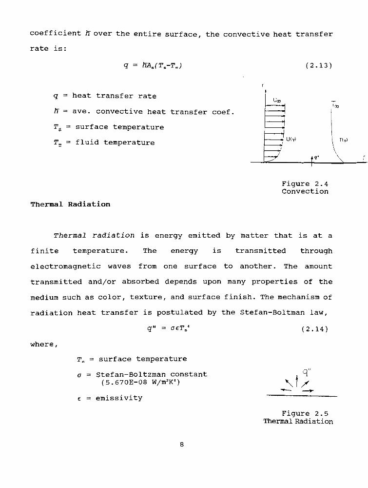
coefficient h over the entire surface, the convective heat transfer
rate is:
g= h~As(Ts-TJ (2.13)
q= heat transfer rate
h~
= ave. convective heat transfer coef
Ts= surface temperature
T = fluid temperatureU(v>
Tr
T(-y)
X
Thermal Radiation
Figure 2 . 4
Convection
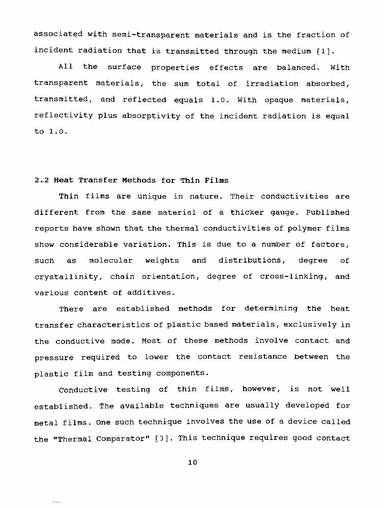
Thermal radiation is energy emitted by matter that is at a
finite temperature. The energy is transmitted through
electromagnetic waves from one surface to another. The amount
transmitted and/or absorbed depends upon many properties of the
medium such as color, texture, and surface finish. The mechanism of
radiation heat transfer is postulated by the Stefan-Boltman law,
q"=
aeTs4
(2.14)
where,
Ts= surface temperature
o - Stefan-Boltzman constant
(5.670E-08 W/m2K4)
e =
emissivity
q"
Figure 2.5
Thermal Radiation

The maximum radiation heat flux may be emitted from an ideal
surface (black-body). The emissivity of a black-body is 1.0 and
anything less than ideal (grey body) will be a fraction of that
parameter [ 1 ] .
The net radiation between two surfaces is of more practical
significance. The net rate of radiation is given by
gnet=
aeAs(Ts*
-
Tsur4J (2.15)
Figure 2 . 6
Net Radiation
where Tsur is the surrounding temperature and As is the area of the
surface in question.
Although we have focused on radiation being emitted by a
surface, irradiation may originate from emission or reflection
occurring at other surfaces. A surface has three basic irradiation
properties consisting of absorptivity, reflectivity and
transmissivity .
Absorptivity is the fraction of irradiation that is absorbed
by the surface and reflectivity is the fractional amount that is
reflected from the surface. On the other hand, transmissivity is
associated with semi-transparent materials and is the fraction of
incident radiation that is transmitted through the medium [ 1 ] .
All the surface properties effects are balanced. With
transparent materials, the sum total of irradiation absorbed,
transmitted, and reflected equals 1.0. With opaque materials,
reflectivity plus absorptivity of the incident radiation is equal
to 1.0.
2.2 Heat Transfer Methods for Thin Films
Thin films are unique in nature. Their conductivities are
different from the same material of a thicker gauge. Published
reports have shown that the thermal conductivities of polymer films
show considerable variation. This is due to a number of factors,
such as molecular weights and distributions, degree of
crystallinity ,chain orientation, degree of cross-linking, and
various content of additives.
There are established methods for determining the heat
transfer characteristics of plastic based materials, exclusively in
the conductive mode. Most of these methods involve contact and
pressure required to lower the contact resistance between the
plastic film and testing components.
Conductive testing of thin films, however, is not well
established. The available techniques are usually developed for
metal films. One such technique involves the use of a device called
the "ThermalComparator" [3]. This technique requires good contact
10

between a hemispherical testing tip and the film. This contact
generally leaves an indentation on the film surface due to the
creation of a high pressure point during testing.
Since some of the films tested in this study are constructed
of a compressible cavitated core, which can be damaged, techniques
such as the one described above can not be used. As a result, a
non-contact method of determining thermal characteristics was used
in this study. Also, a test at high temperatures should be avoided
since the melting point of plastics is generally low.
In this study the use of a steady-state hot/cold apparatus was
considered first. In order to obtain further information, a model
was developed using the steady-state heat conduction equation for
the temperature distribution in a hot/cold air chamber. Typical
film conductivities of 0.01 to .5 W/mK were assumed along with a
temperature difference of approximately 50C ( Thot-Tcold ) and film
thickness of .05mm (about 2 mils).
Results from the one-dimensional model studies showed that
very small temperature differences across the film are obtained,
even for a film thickness of .5mm. In fact, it was determined that
most materials suitable for such a steady-state hot/cold apparatus
are bulk materials of at least 25 mils thick. The magnitude of
films in this study range from . 5 to 5 mils, most being under 2.5
mils.
Laminated stacks of film to increase the material thickness
for greater testing sensitivity was also considered. But due to
concern for the poor contact between films, lamination effects and
11

difficulty measuring small temperature differences, it was not
further pursued.
The method used in this study consisted of exposing the film
to a hot/cold environment as shown below :
FILM
HOT COLD
Figure 2.7
The film is subjected to a temperature differential in a convective
and radiative environment.
An apparatus called an "Insulated Box"was designed and
constructed from hard insulation. In testing, the box covered with
film at one open side was exposed to a freezer environment and the
temperature variations inside the box were recorded as a function
of time.
After the successful testing of the Insulated Box, a purely
conductive apparatus (Thermal Analyzer) was also designed and
tested. The objective of this testing was to compare the films on
a purely conductive basis. This method is similar to the technique
used by Hoosung Lee [ 4 ] .
The Thermal Analyzer consists of a system employing transient,
one-dimensional heat transfer. Essentially, two aluminum blocks of
different temperatures are at steady state at time t0. After the
two blocks are brought together with a film sandwiched between
them, the resistance to heat flow is determined by measuring the
temperature as a function of time in the top block.
12

3.0 MATERIALS & METHODS
3.1 APPARATUS AND PROCEDURES :
3.1.1 Insulated Box
In order to utilize a noncontact, transient, hot/cold
apparatus, the insulated box was designed (Figure 3.1). The box was
insulated with two inch rigid insulation on five sides. The top
side was left open for fitting the film sample. Three thermocouples
were equally suspended inside the box along its vertical depth. One
thermocouple was placed very close to the film without touching it
and another at the bottom of the box.
The thermocouple at the bottom served two purposes: first, to
determine when the inside of the box had reached steady-state, and
second, to qualify that the transmission of heat through the rigid
insulation was minimal compared to the transmission through the top
side. The top of the box was fitted with a thin plexiglass plate to
secure films with an adhesive spray glue.
The box with constant temperature air inside was fitted with
the film and placed film side down (to minimize natural convective
effects) inside a freezer approximately at-30
C. The freezer
controls were bypassed to enable the freezer to operate
continuously and reach a steady, maximum, cold potential.
Thermal transmission takes place from the box, through the
film and into the freezer. Temperature, as a function of time, was
recorded until the air inside the box reached the stable freezer
temperature. The freezer temperature adjacent to the film surface
13

was also recorded. The actual response was determined using the
dimensionless parameter:
(T,(t)-
T.)/(Tx(0)-
T.)
The response of the dimensionless parameter vs. time was
plotted for each film. Repeated testing showed good reproducibility
of the data.
The Insulated Box was also used in a series of separate tests
using automobile antifreeze as the internal fluid. The use of a
liquid in the box eliminated any interior radiation effects that
may be present.
PLEXIGLASS
INSULATION
THERMO
COUPLES
1
1
1
1
1
1
iI
10
1
Figure 3 . 1
Insulated box
14

3.1.2 Thermal Analyzer
Using the Hoosung Lee [4] approach, the Thermal Analyzer which
is schematically shown below, was designed.
WEIGHT
NSULATION C2
UPPER AL BLOCK
-
LOWER L BLOCK
/
/ / /
T(c.
Figure 3 . 2
Thermal Analyzer
The actual test apparatus includes a two block system with the
lower block maintained at a constant temperature and the upper
block being in transient response. Both blocks are surrounded by
rigid insulation in order to eliminate heat transfer from the
sides. Therefore, the primary energy transmission is one-
dimensional. The lower block is kept at a constant temperature of
60C by a heat source consisting of a microscope lamp. The top
block was initially at room temperature of about 20C. Two
15

thermocouples were mounted in the blind holes as close to the block
surfaces as possible.
A single film sample was placed onto the top block with a
small amount of high vacuum silicon grease to reduce the contact
resistance between the two mediums. A small amount of weight was
applied to the top block to provide some pressure for good contact.
Tests were performed using identical films to ensure this weight
provided good repeatable responses. The thermocouple mounted in the
bottom aluminum block remained constant throughout testing.
When the blocks were brought in contact, the temperature was
measured as a function of time, until the thermocouple 1 (upper
block) reached the equilibrium temperature of60
C. Consecutive
tests were completed with each film for reliability. Once again,
the dimensionless parameter
( Ttcl(t)-
Ttc2 )/( Ttcl(0)-
Ttc2 )
was used for recording the thermocouple responses . Good
reproducibilty was obtained.
16
4.0 RESULTS AND DISCUSSION
4.1 Insulated Box
All of the films listed in Table 4.1 were tested with the
Insulated Box. The results are organized by the following
classification: cavitated OPPalytes, coextruded oriented
polypropylene, metallized, OPPalyte/metallized and conventional.
OPPalytes vs. Coextruded Oriented Polypropylene
The transient response are shown in Figure 4.1. The comparisons
show that there is no difference between the responses. For
individual or film composite between 1.0 to 2.0 mils, film gauge,
opacity, or composite makeup have no significance.
Metallized vs. Non-metallized OPPalytes
The results of these tests are shown in Figure 4.2. Aluminum foil
and metallized films show a greater insulative barrier than
nonmetallized films (OPPalytes, coextruded oriented polypropylene,
or polyethelene ) . This is indicated by the slower temperature drop
as a function of time.
Metal li zed /OPPalvte
The results from these tests are also shown in Figure 4.2. Tests
were performed with different film positioning as well."In"
denotes the metal side facing inside the box (facing warm air);
whereas,"out" denotes the metal facing out towards the cold
17

environment. The results showed that the insulative protection
depended upon film surface positioning. In comparison, when the
metallized side faced in (ie. warm side), it was less insulative
than when the metallized side faced out (cold space).
Metallized /OPPalyte vs. all others
The metal lized/OPPalyte films were compared to aluminum foil and
nonmetallized films. These results are also shown in Figure 4.2. It
is observed that aluminum foil and metallized/OPPalyte with
metallized facing"out" have essentially the same response.
Although metallized/OPPalyte faced "in" (towards warm space) was
less insulative than aluminum foil or metallized facing "out", it
was still more insulative than any other nonmetallized films.
Conventional films vs. all others
The conventional films responded correspondingly to the other films
of similar structure as shown in Figure 4.3. The transient response
of aluminum foil was very similar as metallized films. Waxed paper
and freezer paper responded like polymer films. Also, foil/paper
responded the same as metal/polymer composite films.
Box Filled with Antifreeze
The transient response of the box filled with antifreeze is much
slower than the box filled with air as shown in Figure 4.4.
Aluminum foil is also more insulative than polyethelyne in this
scenario, repeating the results of the air filled box.
18

cu H
04 bo
IT)
X r*
0)
o \u
4->
>1-H rH
e (0
o 04
orH
a.04
op
(0
X(1)
0o
00 rH
H
B
H
6 rH
o rH
H*.
04<4-l 04O o
(0
<D
iH
0>
<u
0o 0)
c:u m
rHn
a) H n.N H o<D r-i
4) O iH
b a>U,
r-l 0
U
3
h a)
04 304 .C
o ao
0404o
TJ rH 0, X 04$ rH 04 0) 04p a) o o o(8 0 U0 X X
UHJIHf-H 0-H 0BUBO
HlflHOH
fl BH B
1 1 1 ^ ^r 1 1 1 I'
I I I I I
8"0 9'0 *"0 3"0
Ho a
CD B X0) 0Eh CQ
U r4
<D (0
N -H
(V -P
0) -rl
r4 Cb M
oII II
in
o
oto
o
_o
do
c0)
o(0r-i
T3
aB0)Eh
II
EH Eh Eh
a
fl)
cH
2
H
C "M. M. ) / C "M. .1. )
19

O T30) d)
P N
C-H
0) rH
E r^
& <a
H 4J
a <u
B
pH
3
TJC
(U
P
0 04
o
TJ
.5-p
(0 0)O PO >i
C rH
3 (0
_i
*
B
B3rH
(0
<4H
O
(VN
0)
a>
Jh
b
X3
(V
P(0
0oc3
i5 rH
P-H
0) B>1rH IT)
Oan
CM
Jh
3
P ~
H
0 a
B H
(0
c in o*H 0.B H O
< "S'SN P
H >H
H H O.
B H O .
m 5 :
B
a 4
I
aCO
in
_a
oto
aCM
_a
8*0 9"0 VO 2"0
Q
fl]
cH
H
<4H
B*1
B X ga> o oEhOQ.
-* ^ 12o to
N -H
<D P0) -H
>H Cb H
a
E0)Eh
II IIII
Eh Eh Eh
20

Q)
p
BrH
(01" 04
04H O
XJ
H 0)H +J
O A3
<W 00
cH H
B 'H
3 SH
(0 "*
<H H
oTJ
w cQ) JrH
o>1r4
a0) (0
n a0)
r4
X(0
3
H BJH 040 U 0414 0) O
Q) aa -p <o tj3 >404
"
C H
X(0 (0
3 PH 0)
H -H B -H
BBSin
<\ * m <*
rv . .
H H
("j-fj:)
Cz-j;)
aB X<D OEh CQ
a
e^
aj jN -H
<1) -P
r Cb H
aE<DEh
Eh Eh Eh
(A
(1)
cH
H
21

M-H
<u -*N H
0) 0
CD b
JH<H b
H 3
P C
r, H
ITI fe3
fl H
P <H
3 rH
H
T3 E0)
rH(VI
rHr
H
<4H
X w
0 >
ffl(1)
n c
fi) >1
piH
m ID
rH3
1 P
rn0)
n >1
Mr-t
0
-C0<
PH
H
3H
E'D
0)U)
rH
C)rH
>1 .
uJH
CDN
H
(0
0)
CD
b
73
C(0
^r
*
<D
U
3Cn
E0)
Eh
aE X
<D OEh 03
<C
U<D
N
<u
<D -H
JH Cb H
II II
pC0)
o
(0ll
TJ
(0
a
E0Eh
Eh Eh Eh
CO
CD
D
c
CD
E._>
C -jc TJC ) / C -jc JL )
22

Discussion of Results
The general trend of results can be attributed to radiation
properties of the film, specifically emissivity. The insulated box
results emulate the governing eguation of net radiation transfer
between two surfaces and free convection between two surfaces and
surounding air. The convection coefficient, h (W/mK) , is held
moderately constant in the test procedure. Thus, depending on the
given emissivity of the film, surface finish and surrounding
temperatures, the heat transfer rate through the film will be
slower or faster.
Highly polished aluminum surfaces have a very low emissivity
(approximately .05) and high reflectivity; whereas, white or clear
plastic films have an emissivity of about .9 . The low emissivity
of polished aluminum allows for minimal radiation to take place
between the inside and outside film surfaces and its surroundings,
making it an insulative material under these conditions when
compared to polymer films.
When nonmetallized films are used, the absorbed radiation
energy from the inside of the box is transmitted more easily to the
freezer environment due to high emissivity.
Metallized composite films with the metallized surface"out"
(metal facing cold) are more insulative than those with the
metallized surface"in" (metal facing warm). The low emmisivity on
the outside surface contributes to low thermal transmission.
The dominant surface radiation must take place between the
23

outside of the film and the freezer environment, since both
aluminum foil and metallized composite films with the metallized
surface"out"
have very close responses.
For metallized composite films with metallized surface"in"
(metal facing warm) , the transmissivity is zero causing the film to
be more insulative than the nonmetallized opaque films, but the
nonmetal surface facing toward the cold space radiates more energy
making the film less insulative than with the metallized surface
"out".
Effective use of these results can be summarized in the
following manner:
APPLICATION
Quick Freeze
Slow Freeze
Quick Thaw
Slow Thaw
SURFACE POSITIONING
METALLIZED SURFACE
Facing Warm Space
Facing Cold Space
Facing Cold Space
Facing Warm Space
PLASTIC SURFACE
Facing Cold Space
Facing Warm Space
Facing Warm Space
Facing Cold Space
As noticed, depending on the manufacturer's needs and applications,
one can benefit from the use of the films radiative properties.
24
4.2 Thermal Analyzer
The Thermal Analyzer, on the other hand, was experimentally
set-up as purely a one-dimensional, transient conduction apparatus.
This method utilizes a few factors essential for thin film heat
transfer measurements :
1) Quick transient transmission of heat (about 60 seconds for
most films to reach equilibrium) .
2) A conducting medium (aluminum) that has a significant
magnitude of difference in properties to plastic films.
3) A well insulated set-up to minimize convection and
radiation effects.
The results from Thermal Analyzer testing were reproducible.
The weights on top of the upper block produced good contact and
reliable data with no apparent damage to the film. The weight
distributed over the film surface was considered to be on the same
order of magnitude as in packaging applications. A few different
films were initially tested to ensure good reliability of the
Thermal Analyzer results. The initial testing provided a 5%
tolerance in consecutive test runs.
The results from the films tested with this method are shown
in the transient responses of dimensionless temperature and also in
Table 5.1 which also lists gauge, and apparent conductivity
(discussed in next section).
The Thermal Analyzer results are organized in the following
groups: metallized, coextruded oriented polypropylene, cavitated
OPPalytes, OPPalyte/metal composite and other conventional films
25
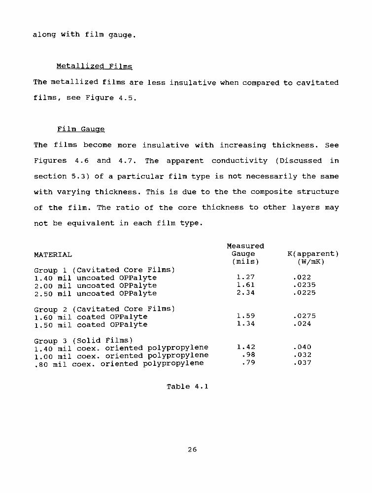
along with film gauge.
Metallized Films
The metallized films are less insulative when compared to cavitated
films, see Figure 4.5.
Film Gauge
The films become more insulative with increasing thickness. See
Figures 4.6 and 4.7. The apparent conductivity (Discussed in
section 5.3) of a particular film type is not necessarily the same
with varying thickness. This is due to the the composite structure
of the film. The ratio of the core thickness to other layers may
not be equivalent in each film type.
MATERIAL
Group 1 (Cavitated Core Films)
1.40 mil uncoated OPPalyte
2.00 mil uncoated OPPalyte
2.50 mil uncoated OPPalyte
Group 2 (Cavitated Core Films)
1.60 mil coated OPPalyte
1.50 mil coated OPPalyte
Group 3 (Solid Films)
1.40 mil coex. oriented polypropylene
1.00 mil coex. oriented polypropylene
.80 mil coex. orientedpolypropylene
Measured
Gauge
(mils)
K( apparent)
(W/mK)
1.27
1.61
2.34
.022
.0235
.0225
1.59
1.34
.0275
.024
1.42
.98
.79
.040
.032
.037
Table 4 . 1
26

01
TJ
C
o
u
<u
in
_ o uj
(0
H ,*
P oH 0C rH
H XJ
rH UCD
CD 3r-t Oan
30 Po c0 (0
E PJh W
CD C
.C OP O
P <4H
(0 O
a a
E ECD CDEh Eh
Cx-x)
27

CD0>
3(00<
<4H
o
p0CD<4H
U
CD
CD
P
ff>
CH
30
Cfl
CO
pH
3 CD01 PCD >,Jh rH
(0
Jh 04CD 04N O>i
HTJ(0 CDC
<
(0
EJh
CD
a .
Eh <ih
vo
^<
CD
Jh
30>
CD qj CD
tttittH H H
(8 (0 (8
04 04 0<04 04 04o o o
S'SSp-p pto d
ooouoo
i-l 1-4 *4
H -H -H
B B B
v o in
H (N <N
o
in
en
oto
incu
o
in
to
Qzou
III
w
UJ
in
H J*P oH 0C -ih J3
H r4
VCD 3r-i 0arH
30 Po cO (0
E PJh
0)
P
P <4H
CO 0
aae sCD CDEh Eh
tl
to CVi
rj-rj:)
C.Z-.Z)
28

CD CDrl-H
Jh
Jh 0CDN TJ
><DrHTJ
ID 3C Jh
<PX
rH (0
(Q 0B OJhCD Ua o
04 04 0404 04 04o o o
TJ TJ TJCD CD QJTJ TJ TJ3 3 3Jh Jh JhP -P PXXXCD CD CD
0 0 0u u u
rA H H
H -H -H
B B B
o o in
co
H H
/*
.^
in
o
in
en
H XP oH OCH
H.O
-t u
9)
CO 3rH Oan
3OP
o c0 IS
E PJh 0
CD CO
P O
P <4-4
ffl o
aa
B B0) CDEh Eh
&
oCO
en
in a
ru zauID
w
o LUCO Z
_ in
-4 o
in
en CD in to cu
("j-rj:)
Ci-D
29
OPPalyte vs. Coextruded Oriented Polypropylene
The cavitated cores in OPPalyte films produce a thermal barrier
better than solid films; consequently, their conductivities (See
Table 4.1) are lower. Also, see Figure 4.8.
Metallized/OPPalyte
The results show very small difference between the
metallized/OPPalyte and the plain OPPalyte films. See Figure 4.9,
Conventional films
Conventional films such as polyethylene and paper products are
not as insulative as OPPalytes. This is due to the thinner gauge
and the absence of a cavitated core.
Other results than those referred to here can be seen in the
Appendix 7.3.
30

to
>
to
(D
P>rH
(0
04
01
o
er
cH
30Gto
10
p
TJ1 1 1
CDP 0) 0)CCD SMH
-4
H H 4J
to eo >h
0 04 04 rH
0 04 04 (0
TJ COOS*
0 O 04
X Jh O O P
88""
O rH
TJ-ht^O
p b a $
u 2 ^
o a o ooSceoOrH 3 3 0
H Jh
CDCD 3-H O0H
3O P
o
o
E PJh
CD
P
P <4H
(0 O
a aE SCD <UEh Eh
I
Cx-Ti)
Cz-D
31

to
>
TJCDN
J
P
CD
E
CD
CA
04
o
TJ
CDP
cu
ooc3
30ato
to
p
3(0
CD
Jh
B
(D O
n m
< CDN
S asU +j
CD m
* C0c
en
CD
Jh30>
H
b
>rH
f-i
CO
r4 >J
P 0H 0ch
H^a
rH Jh
0)
CD 3r^ 0an
3O P
0 c
0 flJ
E PJh CO
CD C, OP O
P *Mm
(0 0
a a
s BCD CDEh -
oII II
I
Ci-Ti)
32

4.3 Statistical Analysis
The Insulated Box and the Thermal Analyzer were analyzed for
confidence to establish significance in the differences seen in the
transient responses.
First, the Insulated Box data was grouped according to film
type: nonmetallized, metallized, nonmetallized/metallized composite
facing"in"
and facing "out". The groups of data were run through
the SAS statistical package for a 95% confidence interval
(tolerance bars) of the cubic line fit used to estimate the dynamic
response.
Results showed that the groupings of data (ie. nonmetallized)
have statistically significant differences, just as first assumed.
The 95% confidence interval bars are drawn about the cubic
estimation in Figure 4.10. The tolerance bars ranged from +0.02
(dimensionless quantity) at the beginning and end of the response
to +0.01 at about 30 minutes into the test run.
The Thermal Analyzer data was grouped using 3 to 4
experimental test runs of each individual film. These data groups
were statistically analyzed using SAS to find 95% confidence
interval on the cubic line estimation of the dynamic responses.
The results showed a maximum of +0.01 tolerance (dimensionless
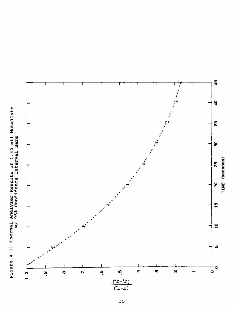
quantity) for each film response. See Figures 4.11 through 4.14.
This data shows good reliability in the test method and a high
level of confidence in the differences established between the
films.
33

CO
p
3U3
CD
01
XoCD
TJ
CD
Pas
<-4
3CO
c
c
o
to
Jh
OS
CD
as
>u
<D
P
C
CD
OcCD
TJH
<+H
c
ou
<#>
IT)
en
CD
>H
3tr>
H
b
10 CO
E E<-a rH
H rH
<4H <4H
TJ ,_^ TJ
CD CD*""
N P N r
H 3 rH C
rH 0 r-i H
COrH rH s
B (0
p CT
as
P IT
H to CD C CD C
<IH E fi rH s H
rH C 0 C o
TJ H 0 (0 0 (0
CD <4H z IH z <4H
N \ \
H TJ TJ rH TJ rH
p
CD
z
rH CD CD (0 CD
rH N N p N
as H H CD iH
p rH rH Z rH
CD rH rH rHs'
g (0 as o
c P P p
o CD CD CD*
z
1
Z
1
Z
!
1
1
l
// '
7 rr
h yA_o
pWI , | I | , |I I , I , I II , | l 1 I I | I M
|M-
8*0 9*0 *"0 Z'U
C "M.Mi ) / C "Jr.jl )
- o
4-
3CH
H
34
CD
P
>r-i
r4
as
PCD
z
l-\ (0H Jh
e CO
CO
o
tf f*.
CO
H >Jh
<4H CD
OPC
W H
prH CD
3 0(0 c
CD CD
TJrH
Jh h
CD cN 0>iOH
as <*>
srH V.
(0 3EJhCD
JCEh
CD
Jh
3
-rfrT
H
m
o
in
en
oeo
(0
in "O
cu ca
u
cu
JO
o IDCU z
in
- o
-
in
01 to in to cu
Cl-TA)
("1-1)
35

TJ
CD
P
CCD-H
u
o to
Jh
TJ as
CD CO
TJ
3 r-i
U as
P >X U
CD P0 CD
U CH
r-i
H CD
s 0c
o CD
*r TJH
H *4
c<4H 00 u
(0 o>
P in
H en
3
to \
CD 3OS
CD
Jh C
CD CDN r-t
>i>iH a(0 oc Jh
< aS-i
r-i -H
as 0
s oh
JhCD
SH
CN
CD
Jh
3T>
("j;-rj;)
("j;-j;)
36

Ci-Ti)
Ci-D
37

CD
ja
asr-*
as
CD
co
10
>1r4
P as
H CO
0
CO r-i
a to
o >u
CD
CTP
rt c
s H
rH CDH CJE c
CDp 13r H
<4H
rH c
0<4H O0
<*>
tO ID
P <T\
r4
3 \CO 3CD
a CD
3u crCD (0
N a
>iOi-i
as CD
C P< H
J2r-\ 2as
EJh
CD
SZ
fr
CD
Jh
3tP
H
b
/
J
I
1
/
/
/
/
r
/
/
in
o
in
to
oCO
to
in ?
eu zoCJ
HIen
o HICU Z
J
/
/
r
/
/
in
-
in
en CD eo in eo cu
38
5.0 MODELING And SIMULATION
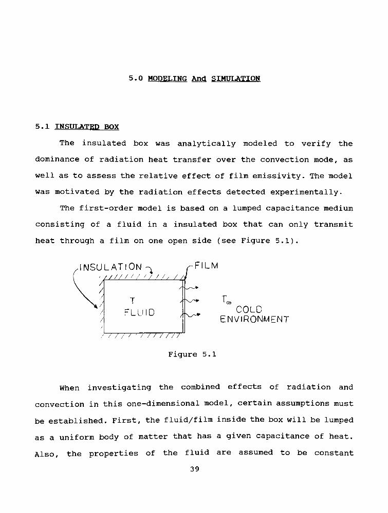
5.1 INSULATED BOX
The insulated box was analytically modeled to verify the
dominance of radiation heat transfer over the convection mode, as
well as to assess the relative effect of film emissivity. The model
was motivated by the radiation effects detected experimentally.
The first-order model is based on a lumped capacitance medium
consisting of a fluid in a insulated box that can only transmit
heat through a film on one open side (see Figure 5.1).
NSULATlON-^
///////// /// //!fFILM
COLD
ENVIRONMENT
////'///////
Figure 5 . 1
When investigating the combined effects of radiation and
convection in this one-dimensional model, certain assumptions must
be established. First, the fluid/film inside the box will be lumped
as a uniform body of matter that has a given capacitance of heat.
Also, the properties of the fluid are assumed to be constant
39

throughout the process .
The first-order differential equation governing the heat
transfer across the film is deduced from energy considerations as:
p C v dT/dt =
-[ h A (Tx-
TJ + eho(Tx4
-
T4J ] (5.1)
(heat flux) = (convective term) + (radiative term)
in which :
p= density (combined)
C = Specific Heat (combined)V = volume
T = Temperature of the bodyh = convection coefficient
A = film surface area
T = ambient surface temperature
e = surface emissivity
a = Stefan-Boltzmann constant
Ti = Temperature of thermocouple 1
The values of the constants in Eq. (5.1) were extracted from
insulated box measurements and convection assumptions as:
V =.00375
m3
A =.022
m2
h = 10 W/mK T=-30C
0. < e < 1 a =5.67*10~8 W/m2K4
Two simulations were performed to qualitatively model the
experimental results.
Case 1 : Air filled box
pconb= 1-0
kg/m3
/c = 1007. J/kgK
Case 2 : Box filled with Antifreeze
pconb= 1110
kg/m3
,C = 2370. J/kgK
40
The simulation results are summarized in Figure 5.2A-C. It is
clear that the larger heat capacitance of the antifreeze filled box
yields a prolonged decay of the dimensionless parameter. The slower
heat transfer rate of the antifreeze versus the air filled box in
Figure 5 . 2A correlates with the experimental responses in Figure
4 . 3 and 4.4.
The correlation for high and low emissivity in the air filled
case ( .9 and.1, respectively) is depicted in Figure 5.2B. The
curve corresponding to an emissivity coefficient of .9 shows a
considerable difference in response. The medium with higher
emissivity (.9) exhibits a considerably faster response, denoting
more heat transfer from the surface.
The modeling also supports the significance of emmisivity- The
percentage of the total heat flux due to the radiative term is
shown in Figure 5.2C. Although the radiative term is not dominant,
it is very significant, especially in free convection.
The above modeling results are derived from a lumped parameter
model and are only intended for qualitative analysis of the heat
transfer process and verification of experimental results. A
higher-order model would have to be developed in order to achieve
quantitative results. The experimental responses strongly suggest
an acute sensitivity of energy transfer to surface properties and
much less sensitivity to specific film gauge or core properties.
Further development of this first-order model is not warranted
since the Insulated Box experiments only show the extreme
difference between metallic and nonmetallic films. In order to
41
further investigate effects of thefilms'
radiative properties,
such as emissitivity, reflectiveness or absorption, more elaborate
experimental work would have to be completed.
42

I
Eh
I
tvT
0.00 0.72 1.44
Time (seconds*103)
Figure 5 . 2A
Theoretical freeze cycle with and without antifreeze,
43

I
Eh
Eh
I
E-7
0.00 0.72 1.44 2.16
Time (seconds*103)
Figure 5.2B
Theoretical freeze cycle with effect of film emissitivity
44

to
p
o
<D
U
<4H
W
CJ
>H
P
as
H
TJ
(0
a
oEh
CD
3a
o03
CO
e =.9
h = io W/mK
0.00 0.72 1.44 2.16 .60
Time (Seconds x 103)
Figure 5.2C
Percent of Heat Flux due to Radiative Effects
45
5.2 FINITE ELEMENT MODELING THEORY
Finite element methods are based on the local application of
variational principles. In a variational framework, a generalized
solution to an operator equation is found by minimizing a giving
functional. The advantage afforded by a variational formulation is
that differentiability properties of solutions are less restrictive
and thereby allow for approximate solutions which are only
piecewise smooth.
The term "variationalformulation" is used contextually to
mean the weak formulation, in which weak refers to the fact that a
function satisfies a boundary value problem in a certain averaged
sense. The differential equation is recast in an equivalent
integral form by trading differentiation between a test function
and the dependant variable. When the differential operator is
symmetric, the weak formulation can be further posed as a
minimization problem for a given functional, I(u). From the
calculus of variations, the minimizing function is the true
solution of the differential equation. For an approximate solution
to a variational problem, the primary variable is approximated by
a linear combination of appropriately chosen functions:
j'-i
46
The parameters c., are determined such that the function u minimizes
the functional I(u), ie. u satisfies the weak formulation [5].
In addition to satisfying a governing equation, the solution
to a boundary value problem must admit specified values on the
boundary of the domain. On the other hand, if the solution or its
derivatives are specified initially (ie. at a set time t0) , then it
is referred to as an initial-value problem. The equations governing
the heat flow in the films represent an initial/boundary value
problem. That is, a combination of the above.
In order to appreciate the fundamental principles of the
finite element method, one must understand the concepts of
functionals and variational operators. Consider the integral
expression
I(u) = faF(x, u,u')dx (5.2)J b
where the integrand F(x,u,u') is a given function of the three
arguments x, u, and du/dx. The value of the integral depends
primarily upon u, hence I(u) is appropriate. The integral in Eq.
(5.2) represents a scalar for any given function u(x). I(u) is
called a functional, since it assigns a value defined by integrals
whose arguments themselves are functions. Mathematically, a
functional is an operator mapping u into a scalar I(u).
A functional l(u) is said to be linear in u if and only if the
relation
l(ou + 6v) =al(u) + Bl(v)
holds for all scalars a, B and functions u and v. A functional of
47
two arguments, B(u,v), is said to be bilinear, if it is linear in
each of its arguments u and v [ 4 ] .
The integrand, F =
F(x,u,u'), depends on the independent
variable x and dependent variables u and u'. An infinitesimal
change in u is called a variation in u and is denoted by <Su. The
operator S will be referred to as the variational operator. The
variation, 5u of a function u, represents an admissible
infinitesimal change in the function u(x). If u is specified on
some portion of the boundary, its variation there must be zero,
since the specified value cannot be varied. The homogeneous form of
the boundary conditions on u must be satisfied by any variation of
the function u. The variation 5u is arbitrary elsewhere on the
boundary .
Boundary conditions play an important role in the derivation
of the approximation function. The variational formulation
facilitates classification of boundary conditions into essential
and natural boundary conditions. For further details, see Reddy [5]
Section 2.2.
In the following, the three basic steps in the variational
formulation of boundary value problems are outlined. Consider the
following differential equation in two dimensions, defined on some
domain n. It is hypothesized that F(x,u,ux,uy) is differentiable,
so that
^d{dFL)d{dFL)=0 withn Qdu dx dux dy duy
48
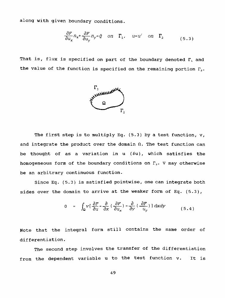
along with given boundary conditions,
dF dF / -n
-nx+~a ny=q on F1,u-u'
on T2duxx duyy y "" li' " " "" X2(5.3)
That is, flux is specified on part of the boundary denoted Tx and
the value of the function is specified on the remaining portion r2.
Q
r2
The first step is to multiply Eq. (5.3) by a test function, v,
and integrate the product over the domain fi. The test function can
be thought of as a variation in u (5u), which satisfies the
homogeneous form of the boundary conditions on r2. V may otherwise
be an arbitrary continuous function.
Since Eq. (5.3) is satisfied pointwise, one can integrate both
sides over the domain to arrive at the weaker form of Eq. (5.3),
0 . (v[^d{dF_)d{_dF_)]Jq du dx duy dy uv (5.4)
Note that the integral form still contains the same order of
differentiation .
The second step involves the transfer of the differentiation
from the dependent variable u to the test function v. It is
49
desirable to transfer the partial derivatives with respect to x and
y (ux & uy) to v so, that only first-order differentiation is
required of both u and v. This results in an equalization of
smoothness for both u and v, and thus is a weaker continuity
requirement on the solution u to the variational problem. In the
process of transferring the differentiation, ie. integration by
parts, we obtain the natural boundary conditions. Eq. (5.4) is now
expressed as
0 - f[v^ +^dF_ +^dF_]dxdy^v{dF_nx+dF_)ds
Jq ou ox ou dy ou Jv auxx
ou
The coefficients of v in the second integral represent the natural
boundary conditions .
The third step in the formulation consists of simplifying the
boundary terms in Eq. (5.5) by applying the specified natural
boundary conditions in the problem statement. This is accomplished
by splitting the two boundary integrals over the subsets rx and T2.
0 .
f[v&+
^F+ cH: dF_]dxdyrv{dF_nx+dF_n)dsf v<Sds
Ja du dx dux dy du Jr2 duxx
ouyy
jt1
dF. dV dF dv 9F_]dxd f v{dF_ dF_
ly Jr2 5ux 3uy
(5.6)
The first boundary integral vanishes, since v is specified (<5u=0)
on T2. The variational formulation thus results in a reduction of
order as well as an automatic imposition of the natural boundary
conditions.
50
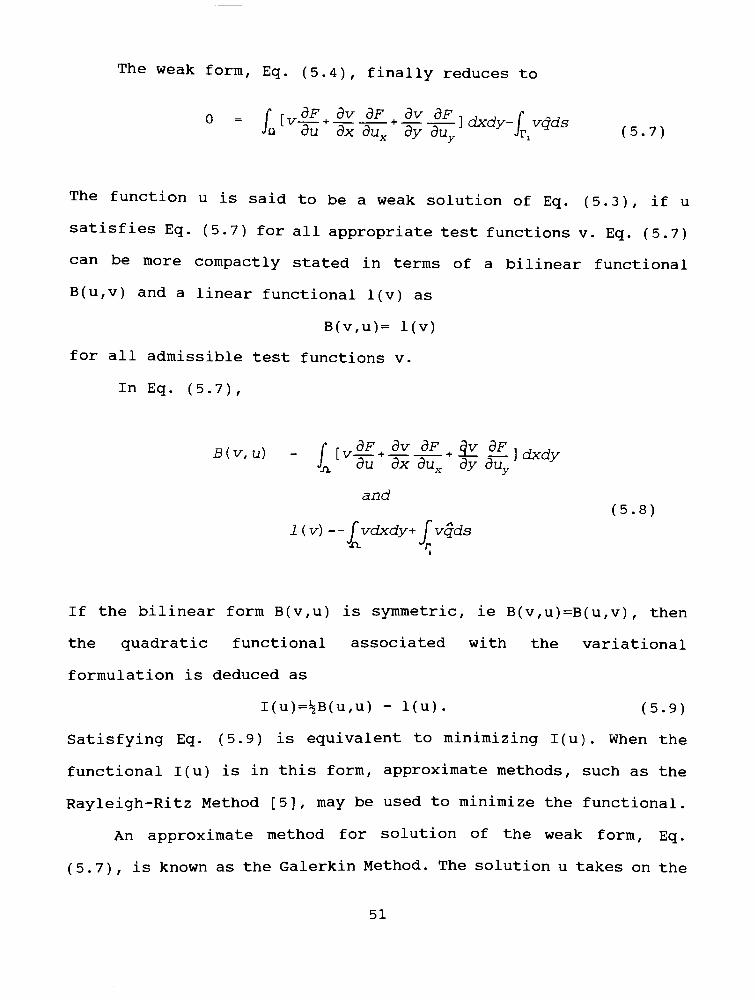
The weak form, Eq. (5.4), finally reduces to
dF.dv dF dv dFf r
dFadv dF dv dF , , . f .
I Lv +3- +^- ] dxdy- \ vqdsJQ du dx du dy du JrL (5.7)
The function u is said to be a weak solution of Eq. (5.3), if u
satisfies Eq. (5.7) for all appropriate test functions v. Eq. (5.7)
can be more compactly stated in terms of a bilinear functional
B(u,v) and a linear functional l(v) as
B(v,u)= l(v)
for all admissible test functions v.
In Eq. (5.7) ,
q/,r ,,\ f r dF dv dF dv dF , , ,
B(v,u) =
|[v-E- +
-5--5 +-35 ] dxdyJn du dx duv dv du\n.
"" ^^w"x ^y ^"y
and
dy
(5.8)
l(v) =- fvdxdy+ J vqds
If the bilinear form B(v,u) is symmetric, ie B(v,u)=B(u,v) , then
the quadratic functional associated with the variational
formulation is deduced as
I(u)=J;B(u,u)- l(u). (5.9)
Satisfying Eq. (5.9) is equivalent to minimizing I(u). When the
functional I(u) is in this form, approximate methods, such as the
Rayleigh-Ritz Method [5], may be used to minimize the functional.
An approximate method for solution of the weak form, Eq.
(5.7), is known as the Galerkin Method. The solution u takes on the
51

form
UN
N
J-l
= Cj*j
in which *.,, the approximating basis functions, must satisfy the
following conditions:
1) They must be well defined and nonzero as well as
sufficiently differentiable as required by the bilinear
form B ( , )
2) Any set {*J(i=l,N) must be linearly independent
3) (*1}(i=l,oo) must be complete.
These conditions guarantee convergence to the solution. For further
discussion of the above conditions, the reader should consult Reddy
[5] Section 2.3. When defining the test function, knowledge of the
anticipated solution as well as satisfaction of any essential or
natural boundary conditions should be taken into account.
The Galerkin approximation is expressed as
un=Ecj*j(x)(5.10)
and the test function is correspondingly written as
m
VE^i (5.11)i-i
52
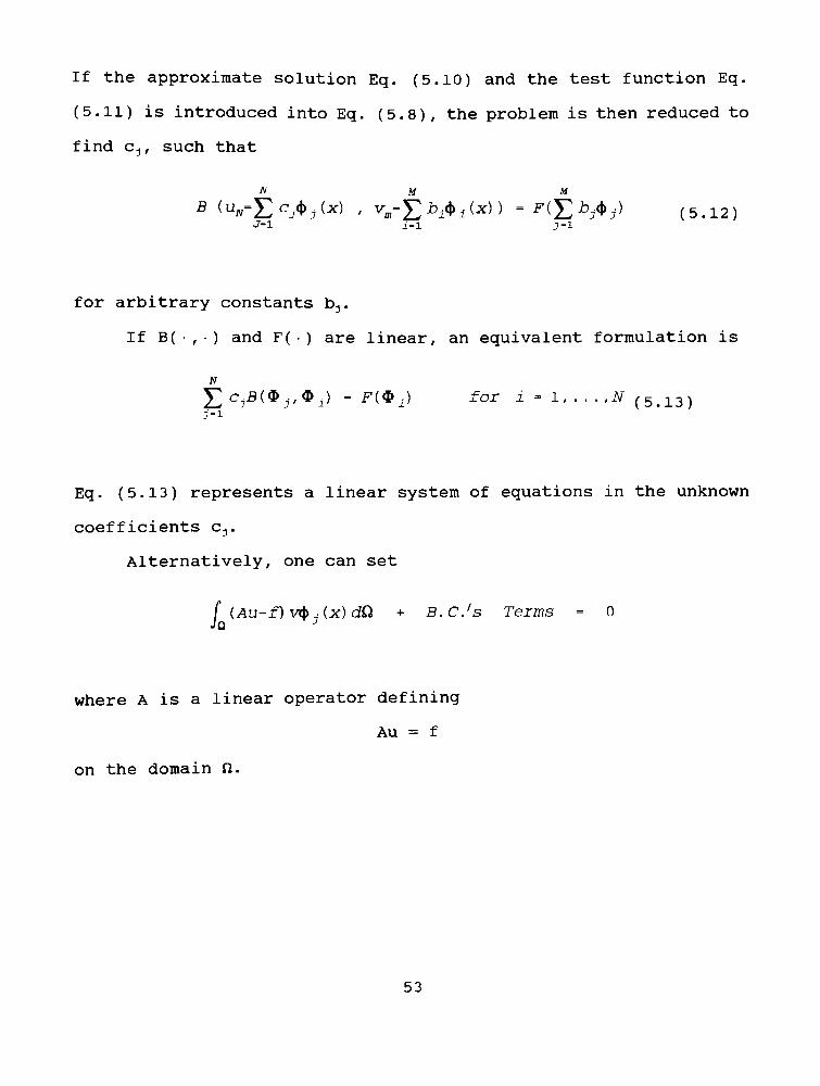
If the approximate solution Eq. (5.10) and the test function Eq.
(5.11) is introduced into Eq. (5.8), the problem is then reduced to
find c-,, such that
B (uN=c,ct),U) , v.-fjb^U)) -Flj^bflj) (5.12)j-i i-i j-i
for arbitrary constants b-,.
If B( , ) and F( ) are linear, an equivalent formulation is
N
c+B(*.,,* ,)= F($i) for i-l #
(5.13)J-l
Eq. (5.13) represents a linear system of equations in the unknown
coefficients c.,.
Alternatively, one can set
f (Au-f)v$Ax)dQJQ
J
+ B.C.'s Terms = 0
where A is a linear operator defining
Au = f
on the domain n.
53

5.3 THERMAL ANALYZER
5.3.1 Galerkin Approximation
The thermal analyzer apparatus (see Figure 3.2) can be modeled
by assuming one-dimensional heat flow, with all heat energy being
transferred through the film from the bottom aluminum block to the
upper block. The film is very thin in comparison to the dimensions
of the aluminum blocks. Further, with the edges being insulated,
the only heat transfer is in the direction perpendicular to the
block surfaces with minimal edge effects. The response is rapid
enough so that any convection taking place on the edge is
negligible. Figure 5.3 below depicts the model schematically with
the associated boundary conditions at the heat source and
insulation barrier.
film
axu
nm
T=60c
Figure 5.3
Mathematically, the film can be represented as a discontinuity
in the material properties of the two conducting aluminum plates.
The conducting composite medium is modeled as two domains divided
by a thin conducting film layer.
54

-['VVW^j-
Dx D2
aluminum film aluminum
Conduction through any medium within the subdomains is
governed by the standard transient heat conduction equation,
FT dT
d*2 at (5.13)
The domains Dt and D2 represent the conducting aluminum blocks.
T(x,t) is the instantaneous temperature distribution within the
domains and
a = k/(pc)
is the thermal diffusivity of aluminum. Separating the two domains
is an extremely thin film layer. The temperature distributions in
the aluminum domains will be approximated using appropriate
Galerkin shape functions, whereas the film temperature profile will
be assumed to be linear, due to the very small thickness of the
film. The instantaneous temperature profile in the apparatus model
is depicted in Figure 5.4.
Figure 5.4
Temperature distribution in the domains.
55
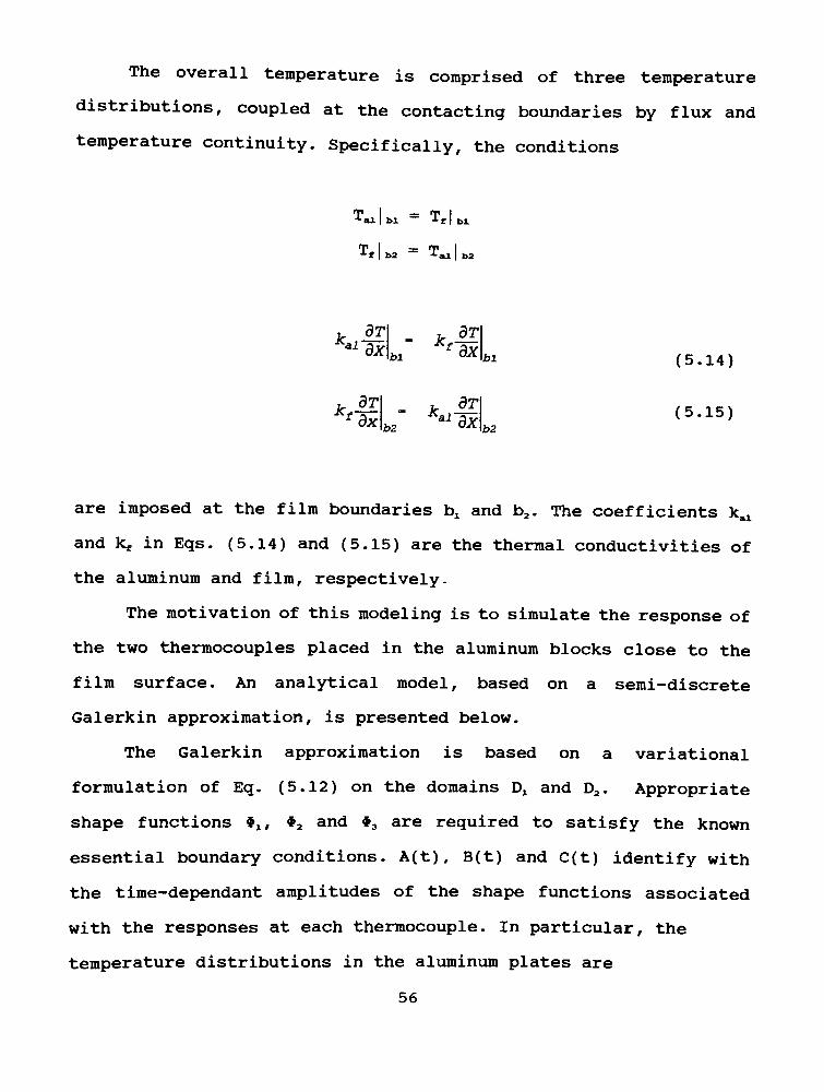
The overall temperature is comprised of three temperature
distributions, coupled at the contacting boundaries by flux and
temperature continuity. Specifically, the conditions
Ti | bi Tt I bl
T* b2= T^ ba
bl
bz
- k il
** (5.14)
(5.15)b2
are imposed at the film boundaries bx and b2. The coefficients k^
and kj in Eqs. (5.14) and (5.15) are the thermal conductivities of
the aluminum and film, respectively -
The motivation of this modeling is to simulate the response of
the two thermocouples placed in the aluminum blocks close to the
film surface. An analytical model, based on a semi-discrete
Galerkin approximation, is presented below.
The Galerkin approximation is based on a variational
formulation of Eq. (5.12) on the domains Dx and D2. Appropriate
shape functions #1# *2 and #3 are required to satisfy the known
essential boundary conditions. A(t) , B(t) and C(t) identify with
the time-dependant amplitudes of the shape functions associated
with the responses at each thermocouple. In particular, the
temperature distributions in the aluminum plates are
56

hypothesized as
T1(x,t)=A(t)*1(x) +60
T2(x,t)=B(t)*2(x) -
C(t)*3(x) +20"
(5.16)
(5.17)
The shape functions *x, *2 and *3 must satisfy the boundary
conditions
x(0,t) =0 & Bi'^L^t)-
C*'3(L2,t) = 0
Transforming the governing differential equation (5.12) into the
variational form, appropriate terms are then integrated by parts.
By implementing the boundary conditions, the equation becomes
simplified. For each domain:
Ll dT, ptv BT, d7\ T
o dx dx dt dx (5.18)
where TA represents the temperature distribution in domain D and
V(x) is the test function associated with the Galerkin method,
specifically *. Substitution of the temperature shape functions,
Eqs. (5.16) and (5.17), into the variational form Eq. (5.18),
results in two ordinary differentialequations for the time-varying
amplitudes:
K1XA + K12A = PSMLJ (5.19)
(5.20)%22 ^23
^32 -^33
B
C
+
^22 ^23
^32 -^33
B
C'Pi
2(0)
3(o)
57

These two differential equations are coupled by continuity of
temperature and flux at the contacting boundaries. That is,
i~dTi
P2 -adx
x-Lj
--2L*^
KK*~ox~ _a_
fl2(0)-A1(I1)-40
x-ij -^a
-t* ink*.
adx
X-0
-Pi
Eqs. (5.19) and (5.20) can thus be expressed as a system of
equations
a xf
KxxA+Ki2^^-'-f [S4>2 (0) -A^ (Lz) -40] -cj), (L)Lf -^a
^11 ^12
^21 ^22
B
C
+
^11 "^12
"21 -"22
B
C
JL--l[B|)2(0)-A<|>1(L1)-40]'
^ ^a
J>2(0)
*3(0)
The initial temperatures of the top and bottom blocks are 20C and
60C, respectively. A linear transformation for the simulated
temperature profiles is utilized to allow for the initial values
A(0) = B(0) = C(0)= 0. The equations are then solved for A(t) ,
B(t) ,and C(t) which results in the temperature profiles
Tx(x,t) =
A(t)$1(x)+60"
T2(x,t) = B(t)#2(x)-
C(t)*3(x) +20
58

The locations of the thermocouples are specified by x=Pi (i=l,2)
Thus the corresponding thermocouple responses are given by:
Ti(px,t) =A(t)*1(p1)+60"
T2(p2,t) =
B(t)*2(p2) -
C(t)#3(p2)+20
The shape functions were chosen as $, =
sin(x) , *2 = l and *3 =
sin(?rx/2*L2) , since these satisfy the known boundary conditions.
The weak formulation on each domain is summarized below.
/dT2dT
(tt-~ +~)vdx=0 Weak formulation
On Dx :
".r<ff-i^*^(5.21)
On D, :
^/>f+f-><*-^<>(5.22)
The respective Galerkin approximations were chosen as
T = A(t)*x +60
,(on DJ
T = B(t)*2-
C(t)#3 + 20, (on D2)
where: *x = sin (x) and
*2 = 1
$3 = sin (?rx/2*L2) .
59
The shape functions * are substituted for v in Eqs. (5.21) and
dT,(5.22). Since
dx=^4>i and -^l=BcJ)/2-aj)/3
dx, it follows that
fLl
(a^Vi^^M^) dx =
P^ (Lx)Jo
fL2(a2(B<l)/2-Qj)/3)ct)/i+(Bcj)2 +Qt>3)<|)Idx = pfotiO)) for i-1,2JQ
(5.23)
(5.24)
Since the temperature distribution in the film is assumed to
be linear, continuity of flux at each contacting surface requires:
*3T>
^al~
dx
-
kJ*- *.
^2val~
dx
Now : ka^-adx
kf=
kal(fltJ)2(0)-A(|1(J1))-40)
X-Z^
So , P2- a
dT
dxX-I^
(5.25)
Integrating Eqs. (5.23) and (5.24) :
On Dx:
AafLlcos2 (x)dx +
A^'sin2
(x) dx = P^sin (L2
Aa[iLl +-isin(2L1)]+A[^-L1-^sin(2L1)]
V*[jb-Asin(L1) -40] sin(L1) (5.26A)
60

On D2:
Integrating with respect to *2:
fNs-Csint-^n-idx = p2-iJo 2L-,
. 2L, aKfBL2-C
2=- X_ [B-Asin(L,) -40]
71 ^ai^f
Integrating with respect to $3:
a(^)2cf^cos2(^)dx+f^(JB-Csin(^^).sin(JE^)dx=P12-0
2L-, Jo 2L, Jo 2L, 2L,
7C2 2L2 . L2.-. -a-^C + -B
- - 0
8L2 ti 2
Rewriting the two equations representing D2
^ac+{SL2-^L2).__Ap,
8L22tc2 * (5.26B)
2L2.5__Ji!__c. (5.26C)
Tt (8-ix2)L7 8-7i2
Eqs. (5.26A-C) represent the final form of the equations qoverning
the amplitude variation and are simultaneously solved for A and B.
In the standard form, the coupled first-order system of
differential equations is expressed as
61
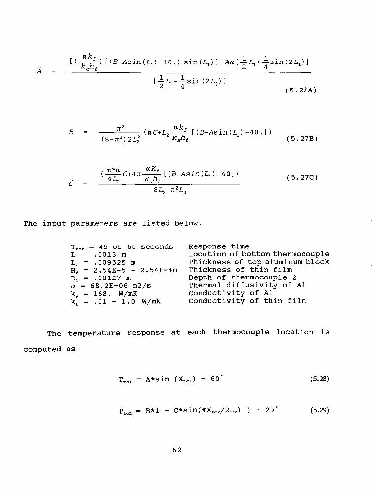
ak
[ l-jr-) i (-B-Asin(L1) -40. ) sin(L1) ] -Aa (-|-L1+-jSin(2Z,1) ]K*f
[^L1~^sxn{2L2)}
(5.27A)
tc2
aicfS = (aC+L,-
-f [(B-Asin(L1)-40.] )(8-tc2)2L22
Mf (5.27B)
C -
{TT2C+^ij-f[{B-ASin{L^ ~4] >(5.27C)
IL2-7t2L2
The input parameters are listed below.
Ttot = 45 or 60 seconds Response time
Lx=
.0013 m Location of bottom thermocouple
L2=
.009525 m Thickness of top aluminum block
Hf= 2.54E-5 - 2.54E-4m Thickness of thin film
Dx=
.00127 m Depth of thermocouple 2
a = 68.2E-06 m2/s Thermal diffusivity of Al
ka = 168. W/mK Conductivity of Al
kf =.01
- 1.0 W/mk Conductivity of thin film
The temperature response at each thermocouple location is
computed as
Ttcl = A*sin (Xtcl) +60
(5.28)
rn = B*l - C*sin(7rXtc2/2L2) ) +20
(5.29)
62
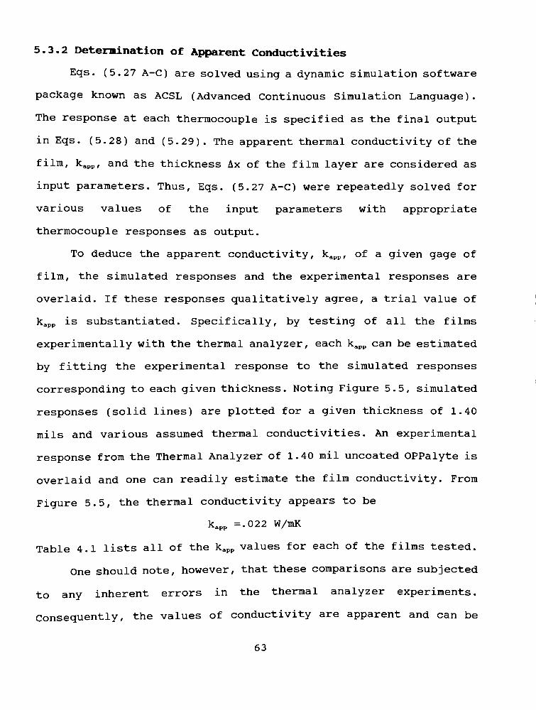
5.3.2 Determination of Apparent Conductivities
Eqs. (5.27 A-C) are solved using a dynamic simulation software
package known as ACSL (Advanced Continuous Simulation Language).
The response at each thermocouple is specified as the final output
in Eqs. (5.28) and (5.29). The apparent thermal conductivity of the
film, kapp, and the thickness Ax of the film layer are considered as
input parameters. Thus, Eqs. (5.27 A-C) were repeatedly solved for
various values of the input parameters with appropriate
thermocouple responses as output.
To deduce the apparent conductivity, kapp, of a given gage of
film, the simulated responses and the experimental responses are
overlaid. If these responses qualitatively agree, a trial value of
kapp is substantiated. Specifically, by testing of all the films
experimentally with the thermal analyzer, each kapp can be estimated
by fitting the experimental response to the simulated responses
corresponding to each given thickness. Noting Figure 5.5, simulated
responses (solid lines) are plotted for a given thickness of 1.40
mils and various assumed thermal conductivities. An experimental
response from the Thermal Analyzer of 1.40 mil uncoated OPPalyte is
overlaid and one can readily estimate the film conductivity. From
Figure 5.5, the thermal conductivity appears to be
kapp =.022 W/mK
Table 4.1 lists all of the kapp values for each of the films tested.
One should note, however, that these comparisons are subjected
to any inherent errors in the thermal analyzer experiments.
Consequently, the values of conductivity are apparent and can be
63

only established on a relative and comparative basis with other
films tested under the same conditions.
Published values of very thin materials vary greatly due to
the variety of experimental techniques, in the Thermal Analyzer,
surface contact between the film and aluminum blocks is one of the
correction factors that must be incorporated to find an absolute
conductivity. Since this contact resistance also exists in real
life applications as well, no correction is made for simulations.
To obtain absolute conductivities one would have to establish
an errorless thermal analyzer and transducer, establish a
thickness-to-conductivity relation for the given samples, or
correlate a surface contact factor derived from a no-film test to
an apparent conductivity.
S
\V\
v\o"
V
o N. \x.
to \N\o"
N. N
\\. ^*
E-." "^Kf=.015
he
X. '4-*^*
"*
!^\o"
Kf=.025^-
^Kf=.020
o(SI
o~
oo
0.00 10.0 20.0 30.0
TIME (SECONDS)
1.40 mil uncoated
OPPalyte (Kf=.022)
40.0 50.0
Figure 5 . 5
System response for selected values of kf,
64

Table 5.1
Material List with apparent k
MATERIAL
1. 1.10 mil uncoatedOPPalyte*'
2. 1.50 mil uncoated OPPalyte
3. 1.40 mil uncoated OPPalyte
4. 2.00 mil uncoated OPPalyte
5. 2.50 mil uncoated OPPalyte
6. 1.60 mil coated OPPalyte
7. 1.50 mil coated OPPalyte
8. 1.00 mil/1.00 mil uncoated OPPalyte
9. 1.10 mil/1.10 mil uncoated Oppalyte
10. metallized/1.50 mil uncoated OPPalyte
11. 1.40 mil coextruded oriented polypropylene
12. 1.00 mil coextruded oriented polypropylene
13. .80 mil coextruded oriented polypropylene
14. Poly coated paper
15. Foil/paper
16. waxed paper
17. aluminum foil
18. chipboard
19. 2.50 mil uncoated OPPalyte/chipboard
20. white pigmented polyethylene
21. polyester
22. high opacity sealable white opaque
23. Hercules white opaque OPP
24. 1.10 mil coated 0PPaLYTE/.75 mil cellephane
25. 1.00 mil coex OPP/1.00 mil coex OPP
26. 1.40 milMetallyte''
27. Hercules metallized white opaque OPP
28. 2.75 mil white low density polyethylene
29. 2.35 mil white low density polyethylene
30a. 7. 5 polystyrene foam
30b. 11.0 mil polystrene foam
31. Metalized polyester/white polyester
32. Poly coated paper
(Ice cream wraps)
(TM) = Trademark
OPPalyte = Trademark name for all Mobil white opaque films
Metallyte = Trademark name for all Mobil metallized films
OPP = oriented polypropylene
* Note : Waxpaper when tested seemed to"melt"
under the thermal
analyzer temperature and any conclusions about waxpaper could be
faulty -
65
GAGE Kapp
(mils) W/mK
1.13 .025
1.55 .026
1.27 .022
1.61 .0235
2.34 .0225
1.59 .0275
1.34 .024
1.89 .032
2.36 .035
1.32 .025
1.42 .040
.98 .032
.79 .037
3.50 .028
2.65 .070
1.35 .050*
.72 .051
16.75 .058
.058
1.50 .075
.59 .032
1.77 .020
1.61 .032
1.82 .031
2.10 .060
1.45 .035
1.61 .042
2.77
2.40 .075
5.95 .029
11. 0(?) .0225
1.97 .070
2.01 .050

5.4 Freezer Enviromngnt-
Response Characteristics Associated with a Freezer Environment
Once the apparent heat transfer parameters of the films are
quantitatively established, one can use this information for
modeling and simulation in environments associated with various
thin film applications.
One specific aspect that is most crucial to the packaging of
frozen dairy products within a typical freezer environment is the
automatic defrost cycle. In the defrost cycle, temperatures rise
above
0
C, where most freezer commodities such as ice cream or
vegetables can momentarily thaw. This defrost cycle can be
potentially detrimental to the package contents. If partially
unfrozen, then refrozen, the package contents will undergo freezer
burn and may be damaged. Frozen liquid items may leak and
eventually refreeze into undesirable shapes.
Manufacturers are seeking the development of films that will
better protect perishable items from permanent damage, such as
freezer burn. The objective of modeling the response of a product
in a freezer environment is to ascertain whether a relative
difference in film properties will actually cause a substantial
improvement in the protection of a product.
The developed model simulates the response of a perishable
item wrapped in various film enclosures. The response profiles were
determined for a variety of film parameters, such as conductivity
66

and thickness, as well as for different freezer environments. The
profiles can be compared to see if any change in the conductivity
results in a substantial change of temperature response within a
package. The expense in the manufacturing of a new composite film
would have to be justified by a definite improvement of protective
property .
The food commodity is first discretized for finite element
modeling. The product domain is bounded by thin layers of film,
generating contact boundary conditions. The different modes of heat
transfer, namely, conduction, convection and radiation are
considered individually to ascertain the relative influence upon
the response of the model. The possible boundary conditions at the
film surface can be numerous, therefore, only a few conditions are
examined in detail. The primary cases are delineated as
1) Pure conduction: The film is in contact with another solid
( ie. food commodity package) .
2) Pure convection: The film is in contact with a fluid (ie.
air) that has an associated convection coefficient, h
(W/m2K) .
3) Convection and radiation: The film exterior, assumed to be
metallized, is exposed to the ambient freezer
environment .
In order to realistically model the thermal response, several
variations in ambient temperature fluctuations were investigated.
These consist of
A) Harmonic : A ramp, constant and fall of temperature to
67

simulate a defrost cycle.
B) Ramp : A constant rise and leveling of temperature to
simulate leaving the frozen commodity exposed to room
temperature .
C) Pulse : Subjecting the frozen item to a warmer environment
for a short period of time then refreezing.
These freezer environment variations are shown in Figure 5.6.
68
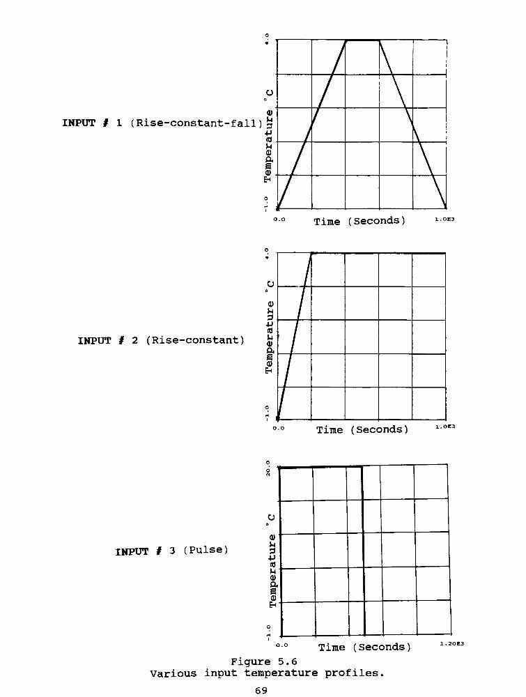
cu
INPUT # 1 (Rise-constant-fall)4-1
as
u
CU
aECUEh
INPUT # 2 (Rise-constant)
INPUT # 3 (Pulse)
Time ( Seconds )
u
cu /as
cu7<D
/V i
Time (Seconds)
fN
9
CUJh
3+
(0
rH
CU
ascufc-l-
0
H
00Time (Seconds)
Figure 5.6
Various input temperature profiles.
69
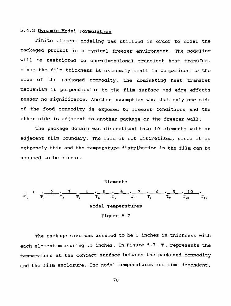
5-4.2 Dynamic Model Formulation
Finite element modeling was utilized in order to model the
packaged product in a typical freezer environment. The modeling
will be restricted to one-dimensional transient heat transfer,
since the film thickness is extremely small in comparison to the
size of the packaged commodity. The dominating heat transfer
mechanism is perpendicular to the film surface and edge effects
render no significance. Another assumption was that only one side
of the food commodity is exposed to freezer conditions and the
other side is adjacent to another package or the freezer wall.
The package domain was discretized into 10 elements with an
adjacent film boundary. The film is not discretized, since it is
extremely thin and the temperature distribution in the film can be
assumed to be linear.
Elements
1.2. 3-4. 5. 6. 7. 8. 9. 10.
Tx T2 T3 T4 Ts T6 T7 T8 T9 T10 TX1
Nodal Temperatures
Figure 5 . 7
The package size was assumed to be 3 inches in thickness with
each element measuring . 3 inches . In Figure 5.7, TX1 represents the
temperature at the contact surface between the packaged commodity
and the film enclosure. The nodal temperatures are time dependent,
70

governed by the transient heat conduction equation. Once the film
boundary conditions are imposed, the model is quantitatively
represented as a tenth-order system of ordinary differential
equations.
The boundary conditions, described above, couple the
individual equations by requirements of flux continuity and
temperature continuity at element boundaries. The dynamical system
is developed as follows.
The local equation for each individual element is
[ K ]e[ T ] + [ R ]e[T]=[f]
(5.30)
where K is the stiffness matrix, R is the dissipation matrix and f
is the generalized force vector. Expressing the conduction equation
d2x dT
dt2 dt(5.31)
in the weak form over each individual element, the element
equations are given by
a 1 -1
-1 1
h 2 l
1 2
pi
(5.32)
Next, the element matrices are assembled with adjoining
71

element matrices to produce a global system for the entire
discretization .
1-10
-1 2 -1
0-12
h 6
(5.33)
0
2 -1 0
-1 2 -1
0 -1 1
2 10
14 1
0 14
0 Pi1
0
4 1 00
1 4 1
0 1 2
p210
Eq. (5.33), in its present form, cannot be solved, since at
this point there are too many unknowns. The system is made
determinate by applying the initial and boundary conditions, after
which the modified system can be solved.P210
contains the film
boundary condition at the exterior surface and is determined by the
appropriate specifications inherent to exterior interaction through
conduction, convection, or radiation & convection.
The Tx boundary condition contains both Tx(0) and T^O). In the
present case, T1(0)=0, by assuming that node 1 of the commodity
contacts either another commodity at the same temperature or ice at
a fixed temperature. Also, for simplicity, it is also assumed that
Ti(o)=0. The initial value at T(0) can be changed to accommodate
any case by adding appropriately to the right hand side [F],
Eq. (5.32) is put into standard form by premultiplying it with
R"1, to obtain
[R"1
][ K ][ T ] + [ T ] = [R"1
][ F ]
72
from which
[ T ] = -
[R"1
][ K ][ T ] + [R"1
][ F ] (5.34)
The final form of Eq. (5.34) is shown as a system of differential
equations listed a Fortran list file in the Appendix.
73
5.4.3 SnimnaT-y of Freezer Simulation Results
A number of cases were investigated, ranging from different
freezer environments to different modes of heat transfer. All of
the freezer environments were characterized by pulse-like
temperature profiles resulting in a dynamic response represented by
a thermal wave of energy propagating through the medium. As the
thermal wave propagates along the spatial, the amplitude of the
temperature is damped due to the internal energy diffusion within
the package contents. This thermal wave propagation differs from
model to model, depending on the inputed temperature variations and
associated boundary conditions (See Figures 5.8 - 5.10). As
expected, the nodal temperatures closest to the film boundary are
the most sensitive to the input temperature variation.
A change in the primary heat transfer mode on the film surface
or the environmental fluctuation resulted in a different frequency
and amplitude of the propagating thermal wave. It is interesting to
note that a change in thickness or conductivity of the film, given
an input response, results only in an amplitude change of the
thermal wave and not a frequency change. Since the amplitude is
actually the magnitude of temperature, one can comparatively
differentiate the relative barrier properties associated with
various film thicknesses and thermal conductivities. Since the
nodal temperatureclosest to the film is the most sensitive, the
74

thermal barrier properties of different films will be analyzed for
the temperature response at TX1. Recall that node 11 represents the
surface of the product which is in contact with the film enclosure.
The comparison will be instituted as a percent difference in
the peak values of temperature across the film boundary, TX1 and
ambient temperature Tinf. This usually occurs near the end of the
simulation run. In particular,
insulative sensitivity= (T-Tlnf )*100
-Linf
The various film parameters, namely, conductivity and
thickness, are compared as a change in insulative sensitivity. The
results of this simulation are summarized in Tables 5.2 through
5.4. In each table, film gauge is varied along the horizontal row
and film conductivity is varied along the vertical column. The
variations in gauge and conductivity were 1.0, 5.0, 10.0, mils and
.05,.10 ,
1.0 W/Mk, respectively.
Table 5.2 illustrates the insulative sensitivity of particular
films to the pure conduction mode, which represents a package
immediately adjacent to another one. For very thin films (<1.0
mils), there is negligible change in sensitivity for Inputs #1 and
#2. As the film gage increases to 5. mils and then to 10. mils, the
change in sensitivity increases on the order of 10% and 20%,
respectively, as the conductivity increases. Therefore, for
relatively thick films, the value of conductivity is critical.
For lower conductivities (<.l W/Mk), the sensitivity is
increased by 10% as the film gauge is increased from 1 mil to 5 and
75
10 mils. For Kf = l.o W/Mk, there is no apparent change in
sensitivity as the film gauge is increased.
Table 5.3 represents the results obtained for the pure
convection mode. The comparison of this mode to the mode that
includes radiation combined with convection will give a reliable
comparison of the effect of surface radiation on package
protection. This scenario is realized as a package situated on top
of a stack of additional packages, subjected to free (nonforced)
air currents in the freezer. There is no apparent change in
sensitivity with a change of either film parameter. Consequently,
in this freezer environment, a change of film thickness or
conductivity is not significant. Another important factor is the
calculation of the convection coefficient, h. These results have an
h value of approximately 2.5 W/m2K, which corresponds to free
convection. The thermal wave propagation can be analyzed in Figure
5.9. For the response to be sensitive to any of the film
parameters, the convection coefficient must be forced convection,
generally on the order of 150 W/m2K, which is unrealistic.
Table 5.4 summarizes the simulated responses associated with
the combined effects of convection and radiation. This combined
mode significantly effects the temperature response as shown in
Figure 5.10. As was apparent for the case involving pure
convection, the model is insensitive to changes in film gage and
conductivity. The emmissivity factor did not become significant
until Input #3 (Pulse). Although the Pulse Input is severe, the
magnitude of difference in temperature response was only1
c.
76
Radiation coefficients are difficult to estimate. It should be
noted that radiation is a direct function of surface color, finish
and texture. Radiation coefficients are best handled
experimentally, with careful attention paid to environmental
factors.
77

Pure Conduction
DELTAX = 1 mil
Kf =.1
Response at TX Response at Tx
Note
Time (Seconds)
Input same as Convection,
u
CUJh
3+J
as
U
CU
aecuEh
o0
Time ( Seconds )
0Response at T,
/u0
CU )r
3P
as
U(1)
Eh
00
u
cu
u3+J
(C
u
cu
a
ecuEh
Response at T7
J>^sO.o
Time (Seconds) Time (Seconds)1.0E3
Figure 5 . 8
Dynamic responses of nodal temperatures
78

Pure Convection
DELTAX = 1 mil
Kf = 0.1
Input
u
cuu
34->
as
u
cu
a
scu&H
1 : t L
U
CU
u
3
-P
(0
rH
CU
a
ECU&H
Response at TX1
0i
^
K1
Time (Seconds)Time (Seconds)
Response at T10
u
cuu
34->
<C
UCU
ecuEh
/
/
CJ
cu
3+J
<0
rH
CU
aECUEh
Response <it T9
6i
H
O
Time (Seconds)o.o
Time ( Seconds )1-OE3
Figure 5 . 9
Dynamic responses of nodal temperatures
79

Convection and Radiation
DELTAX = 1 mil
e = 0.2
Kf = 0.1
Input
u
cu
u
3
P
as
cua
ECUEh
Response at Tx
~\
Time ( Seconds ) Time (Seconds)1.0E3
Response at T1001
SO0
CU
u3P
as
!h
aECDEh <
H
0
H .
o
Response at T9
0l
CJo
u
3+J
(0
CUa
sCUPh
0
Time (Seconds)Time (Seconds)
Figure 5.10
Dynamic responses of nodal temperatures
80

CONDUCTION
INPUT #1 (HARMONIC)
DELTAX 1 mil 5 mil ILLJPLL
^_05 Tlx= 3.871 Tu= 3.36 Tu= 2.79
T10= 1.13 T10=.889
T10=.638
Tlx= 3.36
T1C=.889
T= 3.675
T1D= 1.037
T= 3.967
Tlo= 1.182
1 Txl= 3.93 TX1= 3.675 T1X= 3.36
T10= 1.165 T10= 1.037 T10=.895
1. TX1= 3.993 TX1= 3.967 T1X= 3.933
Txo= 1.19 T10= 1.182 T10= 1.165
INPUT #2 (RISE-CONSTANT)
DELTAX 1 mil 5 mil 10 mil
K*_
.05T1X= 3.911 TX1= 3.569 TX1= 3.163
T10= 1.57 T10= 1.303 T10= 1.019
1. T1X= 3.996 TX1= 3.978 TX1= 3.953
T10= 1.642 T10= 1.623 T10= 1.603
INPUT #3 (PULSE)
tELTAX 1 mi.1 5 mil 10 mil
.01
T1D=
17.8
9.36 T1D=
11.27
4.517
T1X=
T1D=
7.249
2.506
.05
TX1=
T1Q=
19.95
12.16
Tlx=
T1D=
17.82
9.316 T1Q=
15.80
7.428
1.
T1D=
19.97
13.72 Txo=
19.89
13.26
T =
T =
10
19.78
12.86
Table 5.2
Summary of freezer simulation nodal temperatures,
81

CONVECTION
INPUT #1 (RISE-CONSTANT-FALL)
DELTAX 1 mil 5 mil 10 mil
_K*.
Txx=-.8516 T1X=-.8517 Tlx=-.852
T10=-.9338 T10=-.9339 T10=-.9342
TX1=-.8513 TX1=-.8513 T1X=-.8514
Txo=-.9337 T10=~.9337 T10=--9338
INPUT #2 (RISE-CONSTANT)
DELTAX 1 mil 10 mil
K
.05T11=-.7856 Txx=-.7877
T10=-.9175 T10=-.9184
1.0 Tlx=--7854 Txl=-.8552
Txo=--9174 T10=-.9174
INPUT #3 (PULSE)
DELTAX 1 mil 10 mil
01 Tlx=-.2643 Txl=-.3030
Tlo=--704 T10=--7198
05 Txl=-.2607 Txl=-.2689
Tlo=--7027 Tlo=-.7060
1.0 Tlx=-.2600 Txl=-.2602
TXO=--7024 TXO=-.7025
Table 5.3
Summary of freezer simulation nodal temperatures
82

CONVECTTQN & RADIATION
INPUT #1 (RISE-CONSTANT-FALL)
Emissitiv;Lty e= .2 e=.9
DELTAX 1 mil 10 mil 1 mil 10 mil
K,.05 Txx=-.7968 Txl=-.799 T1X=-.6135 Txx=-.6176
TXO=-.909 Tlo=-.910 Txo=-.8267 Txo=-.8267
.1 Tlx=-.796 Txl=-.798 T1X=-.613 Txx=-.615
TXO=--909 T10=-.909 Txo=-.8267 Txo=-.8267
1. Tlx=--796 Txl=--796 Tlx=-.613 Txx=-.6133
TXO=--9092 TXO=-.9092 Txo=-.8266 Txo=-.8267
INPUT #2 (RISE & CONSTANT)
Emissit:ivit;/e=.2 e=.9
DELTAX 1 mil 10 mil 1 mil 10 mil
K.05 Txl=-.7228 Txl=--7250 Txl=-.8095 Tlx=-.8115
Txo=-.8995 Tlo=-.9006 Txo=-.4792 Txo=-.4846
1. Txx=--7225 Txx=--7227 Tlx=-.8093 Tlx=-.8094
Txo=-.8993 Txo=-.8994 Txo=-.4787 Txo=-.4789
INPUT #2 (PULSE)
Emissit1V1 tye'- =.2 e =.9
DELTAX 1 mil 10 mil 1 mil 10 mil
Kf.05
T1X=.0359
TX1=.0246
Tlx= 1.020 Txx=.9989
Txo=-.5817 Txo=-.5863 T10=-.1813 Tlo=-.1900
.1
TX1=.0365
Txx=.0309
Tlx= 1.021 Txx= 1.011
Txo=-.5814 Txo=-.5837 Tlo=-.1809 Txo=-.1852
1. T1X=.0371
T1X=.0365
Txx= 1.022 Txx= 1.021
Txo=-.5812 Txo=-.5814 Tlo=-.1801 TXO=-.1809
Table 5.4
Summary of freezer simulation nodal temperatures,
83

6.0 CONCLUSIONS
In reviewing the results from the experiments and mathematical
modeling, the following conclusions can be stated.
1) A cavitated core film provides better insulation protection
than non-core films in a conductive environment. This
insulative benefit increases as gauge increases.
2) The insulated box experiment and the one-dimensional lumped
parameter model showed that radiation heat transfer is
significant. This significance decreases as the convection
coefficient, h (W/mK), increases.
3) Results show that, metallized films can be utilized more
effectively than nonmetallized films as packaging materials
under conditions of sudden heat or convective/radiative
environments .
4) The thermal analyzer experiment established qualitative
results pertaining to the differences in conductive properties
of various films. These results confirmed initial theories
that a cavitated-core film was more insulative.
84

5) Statistically, the experimental methods proved to be very
reliable. The thermal analyzer experiment could be employed
for other non-packaging films used in a variety of other thin
film applications such as paper copiers.
6) The semi-discrete Galerkin approximation allowed the apparent
conductivities of each composite film to be estimated. Using
the apparent conductivities, one is then able to find response
characteristics of an individual package wrapped in an
insulative film subject to various freezer environments.
7) Mathematical modeling demonstrated how important the
differences in apparent conductivities are in actual freezer
applications. The results from the finite element model showed
that difference in conductivity, when the package is subjected
to a convective and radiative environment, did not contribute
to any substantial insulative differences.
8) The modeling also showed that conduction alone proved to have
insulative benefits with decreasing film conductivity. As the
film thickness increases, these insulative benefits become
more prominent.
85

9) The benefits of this study go far beyond the specific
packaging film results. The 10 element model allows the input
of any boundary conditions (input environments) or package
scenarios that might be of interest. The thermal analyzer,
Galerkin approximation and finite element model can establish
quick and inexpensive results for film conductivities and
significance in a practical environment.
86
7.0 REFERENCES
[1] F.P. Incropera, D.P. DeWitt, Fundamentals of Heat and Mass
Transfer. Second Edition, J. Wiley & Sons Inc., New York, pp.
3-10,35,245, Appendix A, (1985).
[2] U. Grigul, H. Sandner, Heat Conductionr Springer-Verlag, New
York, pp. 1-5, (1984).
[3] C.A. Amsden, "Measurement of The Thermal Conductivity of Thin
Solid Films With a Thermal Comparator," Masters Dissertation,Rochester Institute of Technology, (1988).
[4] H. Lee, "Rapid Measurement of Thermal Conductivity of Polymer
Films,"Rev. Sci. Instrum. . Volume 53, No. 6, June 1982.
[ 5 ] J.N. Reddy ,An Introduction to the Finite Element Method ,
McGraw-Hill, New York, Chapter 2.
87

8.0 APPENDIX
88

8.1 Fortran List Files
ACSL Program : Lumped Conv/Rad Model
Lumped parameter model representative of Insulated Box (5.1).
ACSL Program : KcompGalerkin Approximation of Thermal Analyzer domains (5.3) .
ACSL Program : FreezelOc
Finite Element Model of freezer commodity wrapped in
insulative film with conductive boundary condition (5.4).
ACSL Program : FreezelO
Finite Element Model of freezer commodity wrapped in
insulative film with convective boundary condition (5.4).
ACSL Program : FreezelOr
Finite Element Model of freezer commodity wrapped in
insulative film with convective and radiative boundary
condition (5.4) .
89

"
DETERMINATION OF THE THERMAL PROPERTIES OF POLYMER THIN FILMS"
"DUANE A. SWANSON, MECHANICAL ENGINEERING, ROCHESTER INSTITUTE
"
" OF TECHNOLOGY1990"
"THESIS FOR MASTERS OF SCIENCE "
"Program : ACSL : RIT VAX/VMS
"Lumped parameter model : Insulated Box
"Abstract : This ACSL file solves a model representative
of the Insulated Box. The properties of the air and film"
are averaged together.
it
11
ti
ii
ii
PROGRAM LUMPED CONV/RAD MODEL
DERIVATIVE
C INTERVALn__ _.
CONSTANT
CINT = 1.
DEFINE PRESETVARIABLES"
TSTP = 3600., ...
TEMPIC = 298., ...
TINF = 245.
A =
.0232,
V =.003375
RHO = 1110.
C = 2370. ,
h = 10. ,
eps = 0 ., .
sig= 5.67E-8
TEMPD =-(A/(rho*C*V))*( h*(TEMP -
TINF) + ...
eps*sig*(TEMP**4-
TINF**4))
ii INTEGRATE"
TIME = INTEG(1. ,0. )
TEMP = INTEG( TEMPD, TEMPIC)
DLESS = (TEMP-TINF)/(TEMPIC-TINF)ii SPECIFY TERMINATION
CONDITION"
TERMT(T.GE.TSTP)
END $" OF DERIVATIVE"
END $" OF PROGRAM"
90
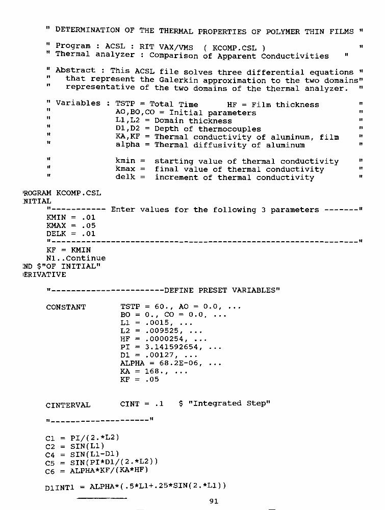
"DETERMINATION OF THE THERMAL PROPERTIES OF POLYMER THIN FILMS
"
"Program : ACSL : RIT VAX/VMS ( KCOMP.CSL )
"
"Thermal analyzer : Comparison of Apparent Conductivities
"
"Abstract : This ACSL file solves three differential equations
"
that represent the Galerkin approximation to the two domains"
representative of the two domains of the thermal analyzer."
"Variables
u
it
ii
ii
u
it
11
11
TSTP = Total Time HF = Film thickness
AO,BO,CO = Initial parameters
L1,L2 = Domain thickness
D1,D2 = Depth of thermocouples
KA,KF = Thermal conductivity of aluminum, film
alpha = Thermal diffusivity of aluminum
kmin =
starting value of thermal conductivitykmax = final value of thermal conductivity
delk = increment of thermal conductivity
11
11
it
n
it
11
'ROGRAM KCOMP.CSL
INITIAL
h
KMIN =
KMAX =
DELK =
01
05
01
Enter values for the following 3 parameters
KF = KMIN
Nl. .Continue
IND $"0FINITIAL"
IERIVATIVE
-DEFINE PRESETVARIABLES"
CONSTANT TSTP = 60.,
AO = 0.0,
BO = 0 .,
CO = 0 . 0,
LI =
.0015, . . .
L2 =
.009525, . . .
HF =
.0000254, . . .
PI = 3.141592654, . . ,
Dl =.00127,
. . .
ALPHA = 68.2E-06, . . ,
KA = 168. , ...
KF =.05
CINTERVAL CINT =.1 $ "Integrated Step"
CI = PI/(2.*L2)
C2 = SIN(Ll)
C4 = SIN(Ll-Dl)
C5 = SIN(PI*D1/(2.*L2))
C6 = ALPHA*KF/(KA*HF)
D1INT1 = ALPHA*(.5*L1+.25*SIN(2.*L1))
91

D1INT2 = ( .5*L1-.25*SIN(2*L1) )
D2C1 =
ALPHA*PI**2/(8*L2)D2C2 = (8*L2 -
PI**2*L2)/(2*PI**2)
D3B1 =
ALPHA*PI**2/((8-PI**2)*L2)D3B2 =
2*PI/(8-PI**2)D3B3 = 2*L2/PI
ADOT = ((C6*(B-A*C2-40.))*C2 - A*D1INT1 )/DlINT2
CDOT = ( 2/PI*C6*(B-A*C2-40. ) + C*D2C1 )/D2C2
BDOT = ( D3B2*C6*(B-A*C2-40. ) + C*D3B1 )/ D3B3
it
INTEGRATE "
A = INTEG(ADOT,AO)B = INTEG(BDOT,BO)C = INTEG(CDOT,CO)
"Temperature distribution in domain"
TCI = A * C4 + 60.
TC2 = B - C*C5 + 20.
"Dimensionsless parameter"
DLESS = (TC2-TC1)/(19.98-TC1)
it SPECIFY TERMINATION CONDITION"
TERMT(T.GE.TSTP)
END$"
OF DERIVATIVE"
TERMINAL
CALL LOGD ( . TRUE . )KF = KF + DELK
IF( KF .LE. KMAX) GO TO Nl
END $"OFTERMINAL"
END $"OF PROGRAM
"
92

DETERMINATION OF THE THERMAL PROPERTIES OF POLYMER THIN FILMS
Program : FreezelOc :
Programmer : Duane A.
ACSL : RIT VAX/VMS
Swanson
Abstract : The ACSL program solves a system of ten differential
equations that represent a Finite Element Model designed to
estimate the transient heat transfer of a frozen commodity
wrapped in an insulating film and subjected to various inputs.
PROGRAM FREEZEC
DERIVATIVE
it DEFINE PRESETVARIABLES"
CONSTANT
CINTERVAL
TSTP = 1200.,...
T20 = -1. , . . .
T60 = -1. ,T10O= -1. , .
T30 = -1. ,T70 = -1. ,
T40 = -1. , T80 = -1. ,
T50 = -1. ,T90 = -1. ,
HE =.015, . . .
DELTAX = 2.54E-05,...
PI = 3.14159, . . .
ALPHA = 3.09E-07, . . .
KF = 1.0,...
TAVE = -1.,. . .
TAMP = 5 . ,. . .
RHOC = 3.33E6
CINT = 1.
T110=-1.01,
CI = ALPHA/ (HE)
C2 = 6./(HE*100.)
MT = T/60
" Various enviromental inputs the model can be subjected to. "
"CASE 1 SINUSOIDALINPUT"
"TINF = TAVE + TAMP*SIN(T*3.14159/600)"
"CASE 2 STEP INPUT"
"Y = PULSE(0. ,1200.
"X = PULSE (400. ,2400.
Z = PULSE( 600.,3600. ,400.)
"
"TINF = TAVE + .75*Y*MT+ X*5,
"CASE 3 PULSE INPUT"
y = PULSE(0. ,1200. ,600. )
TINF = TAVE + Y*MT
93
- ( .75)*Z*(MT-10.)
"

11TINF CASE 3 RISE INPUT "
"TINF = TAVE + MT/2 "
"TINF CASE 4 CONSTANT "
"TINF = 20."
" The boundary condition associated with pure conduction."
PBC=KF* (TINF-T11 ) /DELTAX/RHOC
H System of differential equations representing the finite element model"
T2DOT=C2*(-C1*(60.769*T2-43.078*T3+11.543*T4-3.092*T5+.8287*T6. . .
-.2221*T7+.0595*T8-.016*T9+.0046*T10-.0011*T11) . . .
-.0004*PBC)
T3DOT=C2*(-C1*(-43.078*T2+72.312*T3-46.171*T4+12.371*T5. . .
-3.315*T6+.8883*T7-.2381*T8+.0641*T9-.0183*T10+.0046*T11) . . .
+.0015*PBC)
T4DOT=C2*(-Cl*(+11.542*T2-46.171*T3+73.141*T4-46.393*T5. . .
+12.43*T6-3.33*T7+.8928*T8-.2404*T9+.0687*T10-.0172*T11) . . .
-.0057*PBC)
T5DOT=C2*(-C1*(-3.093*T2+12.372*T3-46.393*T4+73.2*T5-46.41*T6. . .
+12.436*T7-3.333*T8+.8974*T9-.2564*T10+.0641*T11) . . .
+.0214*PBC)
T6DOT=C2* ( -CI* ( . 8267*T2-3 . 315*T3+12 . 431*T4-46 . 41*T5+73 . 205*T6 . . .
-46.411*T7+12.44*T8-3.35*T9+-957*T10-.2392*T11) . . .
-.0797*PBC)
T7DOT=C2*(-Cl*(-.222*T2+.8883*T3-3.331*T4+12.4356*T5-46.411*T6. . .
+73.21*T7-46.427*T8+12.5*T9-3.5713*T10+.8928*T11) . . .
+.2976*PBC)
T8D0T=C2*(-C1*( .0595*T2-.2381*T3+.8928*T4-3.333*T5+12.444*T6. . .
-46.427*T7+73.2692*T8-46.649*T9+13.328*T10-3.332*T11) . . .
-1.111*PBC)
T9DOT=C2*(-C1*(-.016*T2+.0641*T3-.2404*T4+.8974*T5-3.3493*T6. . .
+12.5*T7-46.649*T8+74.098*T9-49.7423*T10+12.435*T11) . . .
+4.145*PBC)
T10DOT=C2*(-C1*( .0046*T2-.0183*T3-t-.0687*T4-.2564*T5+.9569*T6. . .
-3.5713*T7+13.328*T8-49.742*T9+85.6406*T10-46.4102*T11) . . .
-15.47*PBC)
T11DOT=C2*(-C1*(-.0023*T2+.0092*T3-.0343*T4+.1282*T5-.4785*T6. . .
+1.7857*T7-6.6642*T8+24.8711*T9-92.8203*T10+73.2051*T11) . . .
+57.735*PBC)
T2 = INTEG(T2DOT,T20)
T3 = INTEG(T3DOT,T30)
T4 = INTEG(T4DOT,T40)
T5 = INTEG(T5DOT,T50)
INTEGRATE"
94

T6 =
INTEG(T6DOT,T60)T7 =
INTEG(T7D0T,T70)T8 =
INTEG(T8DOT,T80)T9 =
INTEG(T9DOT,T90)T10=
INTEG(T10DOT,T10O)Tll=
INTEG(T11D0T,T110)
TERMT ( T . GE . TSTP )
END$" OF DERIVATIVE "
END$"
OF PROGRAM "
SPECIFY TERMINATION CONDITION"
95

"CASE 3 TINF PULSE INPUT "
Y = PULSE(0. ,1200. ,600. )TINF = TAVE + Y*21
"TINF CASE 4 RISE INPUT "
"TINF = TAVE + MT/2 "
"TINF CASE 5 CONSTANT "
"TINF = 20."
" The boundary condition associated with pure convection on the film.
PBC = KF*HAIR*(TINF-Tll)/(DELTAX*HAIR+KF)/RHOC
" System of differential equations representing the 10 elements.
T2DOT = C2*(-C1*(60.769*T2-43.078*T3+11.543*T4-3.092*T5+. . .
8287*T6 -.2221*T7+.0595*T8-.016*T9+.0046*T10-.0011*T11) . . .
-.0004*PBC)
T3DOT = C2*(-C1*(-43.078*T2+72.312*T3-46.171*T4+12.371*T5. . .
-3.315*T6+.8883*T7-.2381*T8+.0641*T9-.0183*T10+.0046*T11) . . .
+.0015*PBC)
T4DOT = C2*(-C1*(+11.542*T2-46.171*T3+73.141*T4-46.393*T5. . .
+12.43*T6-3.33*T7+.8928*T8-.2404*T9+.0687*T10-.0172*T11) . . .
-.0057*PBC)
T5D0T =C2*(-C1*(-3.093*T2+12.372*T3-46.393*T4+73.2*T5-46.41*T6.
+12.436*T7-3.333*T8+.8974*T9-.2564*T10+.0641*T11) . . .
+.0214*PBC)
T6D0T=C2*(-C1*( .8267*T2-3.315*T3+12.431*T4-46.41*T5+73.205*T6. .
-46.411*T7+12.44*T8-3.35*T9+.957*T10--2392*T11) . . .
-.0797*PBC)
T7DOT=C2*(-Cl*(-.222*T2+.8883*T3-3.3 31*T4+12.4 356*T5-46.411*T6.
+73.21*T7-46.427*T8+12.5*T9-3.5713*T10+.8928*T11) . . .
+.2976*PBC)
T8DOT = C2*(-C1*( .0595*T2-.2381*T3+.8928*T4-3.333*T5+12.444*T6.
-46.427*T7+73.2692*T8-46.649*T9+13.328*T10-3.332*T11) . . .
-1.111*PBC)
T9DOT = C2*(-C1*(-.016*T2+.0641*T3-.2404*T4+.8974*T5-3.3493*T6.
+12.5*T7-46.649*T8+74.098*T9-49.7423*T10+12.435*T11) . . .
+4.145*PBC)
T10DOT = C2*(-C1*( .0046*T2-.0183*T3+.0687*T4-.2564*T5+.9569*T6.
-3.5713*T7+13.328*T8-49.742*T9+85.6406*T10-46.4102*T11) . . .
-15.47*PBC)
T11DOT=C2*(-C1*(-0023*T2+.0092*T3-.0343*T4+.1282*T5-.4785*T6. .
+1.7857*T7-6.6642*T8+24.8711*T9-92.8203*T10+73.2051*T11) . .
+57.735*PBC)
INTEGRATE"
97

T2 = INTEG(T2DOT,T20)
T3 = INTEG(T3DOT,T30)
T4 = INTEG(T4DOT,T40)
T5 = INTEG(T5DOT,T50)
T6 = INTEG(T6DOT,T60)
T7 = INTEG(T7D0T,T70)
T8 = INTEG(T8DOT,T80)T9 = INTEG(T9D0T,T90)T10= INTEG(T10DOT,T100)Tll= INTEG(T11DOT,T110)
ii SPECIFY TERMINATIONCONDITION"
TERMT(T.GE.TSTP)
END$" OF DERIVATIVE
"
END$" OF PROGRAM "
98
DETERMINATION OF THE THERMAL PROPERTIES OF POLYMER THIN FILMSn
" Program : FreezelOr : ACSL : RIT VAX/VMS" Programmer : Duane A. Swanson11
" Abstract : The ACSL program solves a system of ten differential" equations that represent a Finite Element Model designed to11estimate the transient heat transfer of a frozen commodity
" wrapped in an insulating film and subjected to various inputs.
PROGRAM FREEZE10R
DERIVATIVE
CONSTANT
T110= -1. ,
CINTERVAL
DEFINE PRESETVARIABLES"
TSTP = 1000.,...
T20 =-1. , . . .
T60 =
-1.,T10O= -1.,...
T30 =-1.
,T70 = -1.
,
T40 =-1. , T80 = -1.
,
T50 =-1. , T90 = -1.
,
HE =
.015, . . .
DELTAX = 2 . 54E-05
PI = 3.14159, . . .
ALPHA = 3.09E-07, . . .
KF =. 10
, . . .
TAVE =-1 . , . . .
TAMP = 5 .,
. . .
KAIR = 24.3E-03. . . .
HAIR = 2.5, .. .
SIGMA = 5.67E-08, . . .
_~*
* 4.f
G = 9 of
RHOC = 3.33E6
CINT = 1.
CI = ALPHA/ (HE)
C2 = 6./(HE*100.)
C3 = E*SIGMA
MT = T/60.
"Various input responses upon the film's outer boundary. "
"CASE 1 HARMONICINPUT"
"TINF = TAVE + TAMP*SIN(T*3.14159/600)"
"CASE 2 PULSE INPUT"
Y = PULSE(0. ,1200. ,600. )
TINF= (TAVE + Y*21 )
99

11TINF CASE 3 RISE/STEADY INPUT "
"TINF = TAVE + MT/2 "
"TINF CASE 4 CONSTANT "
"TINF = 20."
The boundary condition on the outer element surface."
Radiation/Convection combined."
PBC=KF*(HAIR*(TINF-T11)+C3*( (TINF+273. ) **4 . -(Tll+273 . )**4) )/. .
(DELTAX* (HAIR+4*C3 * (Tll+273 . ) ) +KF ) /RHOC
System of differential equations. "
T2DOT = C2*(-C1*(60.769*T2-43.078*T3+11.543*T4-3.092*T5. . .
+.8287*T6-.2221*T7+.0595*T8-.016*T9+.0046*T10-.0011*T11) . . .
-.0004*PBC)
T3DOT = C2*(-C1*(-43.078*T2+72.312*T3-46.171*T4+12.371*T5. . .
-3.315*T6 +.8883*T7-.2381*T8+.0641*T9-.0183*T10+.0046*T11) .
+.0015*PBC)
T4DOT = C2*(-C1*(+11.542*T2-46.171*T3+73.141*T4-46.393*T5+. . .
12.43*T6-3.33*T7+.8928*T8-.2404*T9+.0687*T10-.0172*T11) . . .
-.0057*PBC)
T5DOT=C2* ( -CI* ( -3 . 093*T2+12 . 372*T3-46 . 393*T4+73 . 2*T5-46 . 41*T6 . ,
+12.436*T7-3.333*T8+.8974*T9-.2564*T10+.0641*T11) . . .
+.0214*PBC)
T6DOT=C2* ( -CI* ( . 8267*T2-3 . 315*T3+12 . 431*T4-46 . 41*T5+73 . 205*T6 . ,
-46.411*T7+12.44*T8-3.35*T9+.957*T10-.2392*T11) . . .
-.0797*PBC)
T7DOT=C2*(-Cl*(-.222*T2+.8883*T3-3.331*T4+12.4356*T5-46.411*T6,
+73.21*T7-46.427*T8+12.5*T9-3.5713*T10+.8928*T11) . . .
+.2976*PBC)
T8D0T=C2*(-C1*( .0595*T2-.2381*T3+.8928*T4-3.333*T5+12.444*T6. .
-46.427*T7+73.2692*T8-46.649*T9+13.328*T10-3.332*T11) . . .
-1.111*PBC)
T9DOT=C2*(-C1*(-.016*T2+.0641*T3-.2404*T4+.8974*T5-3.3493*T6. .
+12.5*T7-46.649*T8+74.098*T9-49.7423*T10+12.435*T11) . . .
+4.145*PBC)
T10DOT=C2*(-C1*( .0046*T2-.0183*T3+.0687*T4-.2564*T5+.9569*T6. .
_3.5713*T7+13.328*T8-49.742*T9+85.6406*T10-46.4102*T11) . .
-15.47*PBC)
T11DOT=C2*(-C1*(-.0023*T2+.0092*T3-.0343*T4+.1282*T5-.4785*T6.
+1.7857*T7-6.6642*T8+24.8711*T9-92.8203*T10+73.2051*T11) .
+57.735*PBC)
., INTEGRATE"
T2 = INTEG(T2DOT,T20)
100
T3 = INTEG(T3DOT,T30)
T4 = INTEG(T4DOT,T40)
T5 = INTEG(T5DOT,T50)
T6 = INTEG(T6DOT,T60)T7 = INTEG(T7DOT,T70)T8 =
INTEG(T8DOT,T80)T9 =
INTEG(T9DOT,T90)T10=
INTEG(T10DOT,T10O)Tll=
INTEG(T11D0T,T110)
itSPECIFY TERMINATION
CONDITION"
TERMT(T.GE.TSTP)
END$" OF DERIVATIVE "
END$" OF PROGRAM "
101

8.2 Additional Responses
Note : Refer to Table 5.1 for thin film identity,
102

M
<D
P
(0
rj
H->
W
to
T3
(1)4-)
(0
CH
E(0
rJ
0
CU
w
c
0aw
CJ
K
r4
CUN
>1H
(0
c
<
(0
e
cEh
in ^ in
CO C\ rH (N CM
=*fc =tfc =tfc =*fc =tfc
i ! !
oto
in
in
o
in
m
O
2O
oO LUm en
m mcu r-
o
CU
in
_l o
in
Clll
~Cl^L)
103

cu
m
c
o
ato
cu
a
ucuN
as
c
<
as
eu
cu
GE*
rH <4H
0
/
71"
/
/
/
/
/
/
/ /
//
/
/
/
/ /
y
/
/
/
/
/
o
x-4
CD CO h- to in m CVJ
in
o
inm
o
m
incu
o
ai
in
in
to
n
co
u
CO
in
l-lr-
Cl-Tl)
Ci-D
104
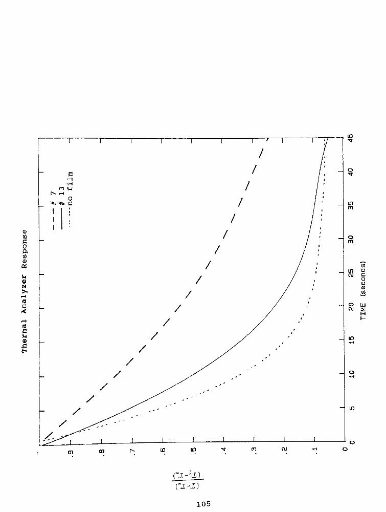
cu
en
co
ato
cu
os
u
CUN
ft
as
c
<
as
eu
cu
GEh
in
TJ
c
a
u
u
in
LU
Ci^il.
Cl-1)
105

cu
to
c
0ato
cu
a
u
cuN
rH
c
<
as
ErH
CU
GEh
Er-\
H
ro rH OH
CM oo (M
0=t*==*fc =*fc c
in
o
inm
oro
01
m TJ
ru C
o
u
u
w"
o 111
ru_:
in
in
Ci-D
i nft