Determining Persistence of Community College Students in Introductory Geology Classes

by

Katrien J. van der Hoeven Kraft

A Dissertation Presented in Partial Fulfillment of the Requirements for the Degree

Doctor of Philosophy

Approved December 2013 by the Graduate Supervisory Committee:

Jenefer Husman, Co-Chair Steven Semken, Co-Chair

Dale Baker David McConnell

ARIZONA STATE UNIVERSITY

May 2014

   

 i

ABSTRACT

Science, Technology, Engineering & Mathematics (STEM) careers have been

touted as critical to the success of our nation and also provide important opportunities for

access and equity of underrepresented minorities (URM’s). Community colleges serve a

diverse population and a large number of undergraduates currently enrolled in college,

they are well situated to help address the increasing STEM workforce demands.

Geoscience is a discipline that draws great interest, but has very low representation of

URM’s as majors.

What factors influence a student’s decision to major in the geosciences and are

community college students different from research universities in what factors influence

these decisions? Through a survey-design mixed with classroom observations, structural

equation model was employed to predict a student’s intent to persist in introductory

geology based on student expectancy for success in their geology class, math self-

concept, and interest in the content. A measure of classroom pedagogy was also used to

determine if instructor played a role in predicting student intent to persist. The targeted

population was introductory geology students participating in the Geoscience Affective

Research NETwork (GARNET) project, a national sampling of students in enrolled in

introductory geology courses.

Results from SEM analysis indicated that interest was the primary predictor in a

students intent to persist in the geosciences for both community college and research

university students. In addition, self-efficacy appeared to be mediated by interest within

these models. Classroom pedagogy impacted how much interest was needed to predict

 

  ii

intent to persist, in which as classrooms became more student centered, less interest was

required to predict intent to persist. Lastly, math self-concept did not predict student

intent to persist in the geosciences, however, it did share variance with self-efficacy and

control of learning beliefs, indicating it may play a moderating effect on student interest

and self-efficacy.

Implications of this work are that while community college students and research

university students are different in demographics and content preparation, student-

centered instruction continues to be the best way to support student’s interest in the

sciences. Future work includes examining how math self-concept may play a role in

longitudinal persistence in the geosciences.

 

  iii

ACKNOWLEDGMENTS

A dissertation can be a lonely endeavor, but I have had the good fortune to have

an incredibly supportive community as I have worked through this project. It is only

appropriate that I acknowledge that this dissertation would not be completed (or even

started) were it not for this community of friends and scholars.

I feel truly fortunate to have a unique and interesting history with each of my

committee members that helped me decide to take the leap into the PhD program. Dale,

if I had not met you with the CISIP project, I may not have realized the quality of

educational research that exists and how incredibly cool metacognition was, which

started me down this path. David, if you had not stood up and asked who wanted to write

a grant with you on that fateful February afternoon in Minnesota, I certainly would not

have been here. Steve, you helped me realize that quality research can and should be

done in geoscience education and is just as important as geological science research.

Jenefer, you inspired me to learn more about motivation that helped explain so much

about how and why my students do what they do. I feel fortunate that I had a committee

who challenged me, held me to a high expectation, but were also positive and supportive.

All of my committee members pushed me to think harder and deeper than I thought

possible, and I feel as though I have grown and benefited through it all.

This research would not be possible without the entire GARNET team including

David Budd, Ann Bykerk-Kauffman, Lisa Gilbert, Jonathan Hilpert, Megan Jones, Laura

Lukes, Ronald Matheney, Dexter Perkins, Jennifer Stempien, Tatiana Vislova, and Karl

Wirth. All of the participating instructors and institutions in the research, and of course

 

  iv

the students who spent their time filling out these surveys, thank you. In particular, I

would like to thank Jon Hilpert for his invaluable assistance with my structural equation

models and helping me to accept and figure out how to deal with the reality of messy data

rather than idealized textbook data. In addition, Laura Lukes was a constant source of

encouragement and support, and asked different questions that challenged my thinking.

I have had a number of friends who have previously been through this process

who were constant sources of inspiration and encouragement. Drs. Merry Wilson, Amy

Leer and Niccole Cerveny all pushed me to keep working when I needed to, but also to

stop and take a break when I was nearing the cliff.

They say timing is everything. Who knew that picking this time to do my Ph.D.

would be the best time because of the incredible community of scholars with whom I

have had the benefit to work and collaborate. To have a writing group who you can trust

to provide critical feedback and encouragement through it all has been the primary reason

I have completed this degree. Heather Pacheco and Kathy Hill have probably read more

versions of this dissertation than anyone else, and for that I am truly fortunate and

grateful. You both inspire me to work harder and expect more of myself.

My supportive husband, Mike Kraft and our loving dogs, Takoda and Kleo were

infinitely patient with me as I had no time to do anything on any weekends for years in a

row. I would be gone for dinners, for walking time, for too much. Thank you for your

patience and keeping me grounded.

 

  v

Lastly, I would like to say a very special thank you to my parents. You helped to

create an environment that encouraged life-long learning, you supported me emotionally

and financially. I can never thank you enough.

Maricopa Community College District provided me with a leave of absence in

order to complete this dissertation, without which I would not have been able to do in

such a timely manner. This research is based on work supported by NSF DUE Award #:

1022980 (part of a collaborative grant), any opinions, findings, and conclusions are those

of the author and do not necessarily reflect the views of NSF.

 

  vi

TABLE OF CONTENTS

Page

LIST OF TABLES ........................................................................................................... viii

LIST OF FIGURES .............................................................................................................x

CHAPTER

1 INTRODUCTION ...................................................................................................1

2 LITERATURE REVIEW ........................................................................................4

Persistence at the College Scale ...............................................................................4

Persistence at the Classroom Scale ..........................................................................8

Persistence at the Individual Scale .........................................................................12

3 HYPOTHESIS & RESEARCH QUESTIONS ......................................................22

4 METHODS ............................................................................................................23

Participants .............................................................................................................23

Measures ................................................................................................................24

Procedure ...............................................................................................................27

5 RESULTS ..............................................................................................................51

Characterizing the Data ..........................................................................................51

Characterizing the Population ................................................................................55

Structural Equation Modeling Analysis .................................................................63

6 DISCUSSION ........................................................................................................86

Differences between Community College and University Students ......................87

Role of Expectancy and Interest in Predicting Intent to Persist .............................89

 

  vii

CHAPTER Page

Role of Instructor ...................................................................................................90

Role of Math Self-Concept in Expectancy for Success .........................................92

Role of Math Self-Concept in Predicting Intent to Persist ....................................93

Interest as a Mediator .............................................................................................95

Limitations of the Study.........................................................................................97

7 NEXT STEPS & IMPLICATIONS .....................................................................100

REFERENCES ................................................................................................................105

APPENDIX

A. GEOSCIENCE AFFECTIVE RESEARCH NETWORK (GARNET)

ITEMS..................................................................................................................119

B. MOTIVATED STRATEGIES FOR LEARNING QUESTIONAIRE

ITEMS (MSLQ) ...................................................................................................123

C. MATH SELF-CONCEPT ITEMS .......................................................................125

D. REFORMED TEACHING OBSERVATION PROTOCOL (RTOP)

SCALE .................................................................................................................127

E. HUMAN SUBJECTS APPROVAL FROM MARICOPA COUNTY

COMMUNITY COLLEGE DISTRICT AND ARIZONA STATE

UNIVERSITY ......................................................................................................138

 

  viii

LIST OF TABLES

Table Page

4.1 Detailed breakdown of methods and instruments applied to the research

questions ...................................................................................................................25

4.2 Fit indices reported in this research with cut-off values and affordances and

constraints of each .....................................................................................................46

5.1 Results from Chi-squared tests comparing R1S and CCS to the R1F and CCF ...........51

5.2 Results from t-test comparing R1S and CCS with bootstrapped population of R1F and

CCF ............................................................................................................................52

5.3 Descriptive statistics of the four major subscales used for this research at each

institution ..................................................................................................................53

5.4 Measurement invariance omnibus test all variables ...................................................54

5.5 Measurement invariance tests for continuous items ...................................................55

5.6 Comparison of previous science and math courses taken by students enrolled at

different institutions ..................................................................................................59

5.7 Reasons for students enrolling in the course ..............................................................61

5.8 Bivariate correlations among items used for SEM analysis with R1 and CC

students .....................................................................................................................62

5.9 Parceling of subscale items for SEM analysis ............................................................63

5.10 Results of CFA comparisons between different RTOP classrooms .........................67

5.11 SEM regression results for different RTOP ranked classrooms in both original

analyses and post-hoc results ....................................................................................68

 

  ix

Table Page

5.12 CFA results for continuous variables of Self-Efficacy, Math Self-Concept and

Control of Learning Beliefs ......................................................................................75

5.13 SEM regression results for the full model of Interest, Self-Efficacy, Math Self-

Concept and Control of Learning Beliefs in predicting intent to persist .................77

5.14 SEM results when interest variable was removed from original models .................81

5.15 SEM results where interest was removed from RTOP classroom models ...............84

5.16 SEM regression results for different RTOP ranked classrooms where interest was

removed ...................................................................................................................84

5.17 SEM results where interest was removed from the final model ...............................86

6.1 Predictors of intent to persist in different RTOP classrooms .....................................90

6.2 Relationships in SEM with math self-concept ...........................................................94

 

  x

LIST OF FIGURES

Figure Page

4.1 Illustration of the basic structure of a measurement model for SEM .........................33

4.2 Illustration of the basic structure of a structural model for SEM ...............................34

4.3 Proposed measurement model for this research project .............................................35

4.4 Proposed structural model for this research project ...................................................35

4.5 A decision map for SEM analysis ..............................................................................37

4.6 Adapted model of mediation from Baron and Kenny (1986) ....................................50

4.7 Adapted model of moderation from Baron and Kenny (1986) ..................................50

5.1 Students ages represented at both institutions reported as percentages .....................56

5.2 Students at the community college are more likely to be undeclared or non-stem

relative to their R1 counterparts .................................................................................57

5.3 The range of races for participants in this study ........................................................58

5.4 Reasons students selected to enroll in the course .......................................................60

5.5 Structural model for CCF responses predicting intent to persist based on self-

efficacy, control of learning beliefs and interest ........................................................65

5.6 Structural model for R1F responses predicting intent to persist based on self-efficacy,

control of learning beliefs and interest .......................................................................66

5.7 SEM for high RTOP CCF classrooms ........................................................................69

5.8 SEM for middle RTOP CCF classrooms ....................................................................70

5.9 SEM for high RTOP R1F classrooms .........................................................................71

5.10 SEM for middle RTOP R1F classrooms ...................................................................72

 

  xi

Figure Page

5.11 SEM for low RTOP R1F classrooms ........................................................................73

5.12 CFA model for CCS population of just continuous items ........................................75

5.13 CFA model for R1S population of just continuous items .........................................76

5.14 Final SEM for CCS classrooms ................................................................................78

5.15 Final SEM for R1S classrooms .................................................................................79

5.16 Structural model for CCF with interest removed ......................................................80

5.17 Structural model for R1F with interest removed .......................................................81

5.18 Structural model for CCF with interest removed in high RTOP classrooms ............82

5.19 Structural model for CCF with interest removed in middle RTOP classrooms ........82

5.20 Structural model for R1F with interest removed in high RTOP classrooms ............82

5.21 Structural model for R1F with interest removed in middle RTOP classrooms ........83

5.22 Structural model for R1F with interest removed in low RTOP classrooms .............83

5.23 Final structural model for CCS with interest removed .............................................85

5.24 Final structural model for R1S with interest removed ..............................................85

 

  1

Introduction

Setting the Stage

In an effort to understand why issues of equity and access to the sciences are

important, it helps to consider how the population in the United States is predicted to

change and how that will impact future job vacancies in the sciences. By 2050, the

current underrepresented population (Hispanic, African-American, Asian and mix of 2 or

more races) will comprise nearly half of the population (Day, 1996), as a result, the

current majority White population will no longer be the dominant contributors to the job

market. If Science, Technology, Engineering and Mathematics (STEM) jobs currently

held by the majority are not replaced and filled by individuals in the growing minority

groups, the nation faces a possible crisis. If the current shortages in the STEM workforce

were filled with representative members of underrepresented groups as currently reflected

in the U.S. population, there would be no shortfall in the workforce (May & Chubin,

2003), the challenge for meeting that demand however is our current post-secondary

programs are not producing enough STEM majors of any ethnicity to fill the demand

(Carnevale, Smith & Strohl, 2010).

In addition to addressing the needs of the nation, STEM careers can provide

opportunities of access and equity for underrepresented minorities (URM’s). Access is

defined as the opportunity for anyone, regardless of ethnicity, sex, socioeconomic status

(SES), disability, age or other demographic category to achieve a college education. This

is possible due to changing policies from a merit-based access (those who have

historically had the ability and the societal opportunities, for example White, Protestant,

 

  2

upper class males in the U. S.) to an equity-based access, in which opportunities are

available to help create a level playing field even if those background experiences are not

the same, for example, need-based financial support (Clancy & Goastellec, 2007). The

importance for providing equitable access is due to the advantages that come for those

who are able to obtain a college education. For example, individuals who have a post-

secondary education are more likely to have careers where on-the-job training allows for

skill development that results in adaptability to changes in technology and job demands

(Carnevale, et al., 2010). Current job projections indicate that more than 90% of all

STEM jobs will require at least some college within the next decade (Carnevale, et al.,

2010).

Some have suggested that a possible source for increasing URM’s in STEM

overall, as well as within the geosciences, is from the community colleges (e.g.,

Hagedorn & Purnamasari, 2012; Holdren & Lander, 2012; National Research Council

and National Academy of Engineering, 2012; van der Hoeven Kraft, Guertin, Filson,

MacDonald & McDaris, 2011a). Community colleges are well situated to potentially

provide a greater pool of URM’s for STEM, since students from community colleges are

generally older (28 vs. 21 yrs. old average age), more diverse (42.7% minorities vs.

37.5% minorities), and have more first generation college students (42% vs. 30%) than

their four-year counterparts (National Center for Education Statistics [NCES], 2001;

National Science Foundation [NSF], (2009); American Association of Community

Colleges [AACC], 2012). In addition, there is evidence that 44% of all students with

Science and Engineering (S&E) bachelor’s degrees have taken some of their coursework

 

  3

at the community college (Tsapogas, 2004). However, there are tremendous hurdles for

students from community colleges to over come in order to become STEM majors. Only

17% of students who receive an associates (2-year) degree go on to complete a 4-year

degree (Carnevale, et al., 2010). A recent report on geoscience majors indicated that only

14% of all students with a B.A. or B.S. in the geosciences took a geoscience course at the

community college (Wilson, 2013).

Developmental education is a growing role that community colleges fill in

preparing students for their academic transfer. Developmental education (also known as

remedial, compensatory, preparatory, or basic skills studies) are the courses that students

need to take when they enter college that are below the college level coursework, and

therefore are not transferrable to four-year institutions (Cohen & Brawer, 2008; Hagedorn

& DuBray, 2010). Ninety-eight percent of all community colleges provide some form of

developmental education (Parsad & Lewis, 2004).

One of the most problematic developmental courses, especially for STEM majors

is math. In one study, more than 76% of all students with a desire for a career in STEM

required some form of pre-gatekeeper math class (a class that is needed prior to the

college-level course that is part of an actual STEM program), 36% of whom were at the

developmental level (Hagedorn & DuBray, 2010). While 75% of students were able to

pass their first math course in the trajectory of getting to college-preparedness, it took

repeated attempts for some of them to do so (9-17% depending on the course). For these

students, the developmental courses are gatekeeper courses. If a student enters the

community college at the developmental level, it can take four or more semesters of

 

  4

successfully passing each course to get to the math courses that are transferrable to a

four-year institution and counted toward a STEM degree (Hagedorn & DuBray, 2010).

The difference between students who require a remedial course and those who do not,

can be the difference between successfully transferring to a four-year institution and

completing within a six-year time frame and taking much longer, if completing at all

(Bailey, Jenkins, & Leinbach, 2005). Developmental math courses have been described

as, “a firing squad,” in response to the attrition that occurs (National Research Council

and National Academy of Engineering [NRC & NAE], 2012; p. 32). Math is a major

hurdle for students interested in entering STEM.

Literature Review

The following presents the current research on persistence at the college,

classroom and individual scale. This literature review helps to set the stage for what gaps

remain in the literature about persistence in STEM programs at the college level,

particularly, community college students in the geosciences. Geosciences are defined as

including geology, physical geography, meteorology, oceanography, and planetary,

Earth, and environmental sciences.

Persistence at the College Scale

Tinto (1993) established a model for explaining persistence among students in

college in general. Particularly important are issues of academic and social integration.

Tinto (1993) describes the importance of both opportunities for students to be engaged

academically, with a voice in their learning experience and clear goals for their academic

 

  5

success. This academic engagement is enhanced and augmented by the social

interactions. These opportunities for engagement begin in the classroom, and spiral

outside from there. As a student has an opportunity to experience a learning community

in a classroom, s/he is more likely to engage outside of the classroom with both

classmates and the instructor. Tinto argues that this is even more important in institutions

that are commuter/non-residential campuses since students are less likely to have

interactions outside of the classroom (Tinto, 2006). Evidence shows that students at

community colleges are more likely to persist if they engage in learning communities that

offer opportunities to develop social networks at the same time as they are academically

engaged in their learning environment (Tinto, 1997). In addition, these interactions and

feelings of integration are most critical in the first year of college (Tinto, 2006). Most of

the current research done on persistence at the college scale has been at four-year

colleges, very few have occurred at community colleges (Tinto, 2006). As such, this

model may be less appropriate in predicting persistence in STEM for community colleges

students, because students at the community college are potentially different based on

their preparation level and social capital. Community colleges are more likely to have a

higher representation of URM’s because of the affordability, the lower admission

restrictions and developmental education courses, and the flexibility for working with

students who may be working and/or have family obligations (Parsad & Lewis, 2004;

Bailey et al., 2005; Horn & Nevill, 2006; Cohen & Brawer, 2008; Provasnik & Planty,

2008). As a result, community colleges should be of interest for recruiting for STEM

majors, and has been specifically identified by the President’s Council of Advisors on

 

  6

Science and Technology (PCAST) as one of the possible sources for the 1 million new

STEM majors needed to fill the needs of the workforce (Holdren & Lander, 2012).

There are several identified institutional factors that influence persistence in

STEM majors, particularly URM’s. These factors are common to those identified by

Tinto (1993) in his larger persistence model as developing relationships with peers

outside of the classroom through school-sponsored organizations and informal study

groups (Espinosa, 2011). In addition, opportunities for undergraduate research positively

impact persistence, whereas highly selective institutions and those with high ratios of

graduate students to undergraduate students negatively predict persistence (Griffith,

2010; Espinosa, 2011).

While students have hurdles to overcome becoming STEM majors at the

community college, the geosciences have more challenges than most STEM majors.

There are several factors needed for students to choose to become a major: 1) knowledge

and interest in the subject area; 2) earning potential (somewhat mediated by

socioeconomic status); 3) the skill set required to be successful and an ability to

accurately gauge those skills for a given task, and 4) a feeling of a connection to a given

community (Tinto, 1997; Montmarquette, Cannings, & Mahseredjian, 2001;

Harackiewicz et al., 2008).

Geology is a topic that is generally relegated to middle school curriculum and

when taught in high school, is commonly taught as the non-college track Earth Science

course (Lewis, 2008). In fact, enrollment in Earth Science in high school was found to be

the one science course in high school that negatively predicted persistence in STEM

 

  7

majors in college (Maltese & Tai, 2011). As a result, most students receive very little

exposure to the content prior to taking a college-level geology course. Interest

researchers may not agree about the semantics of what different degrees of interest are,

but they generally do all agree that in order to be interested in a topic, one must have

knowledge about it (Krapp, 2002; Hidi & Renninger, 2006). As a result, many students

who choose to become geology majors are those who “discover” it in college. Houlton

(2010) did research on why students choose to become majors, and she categorized them

into three different groups: natives (those who knew about geology prior to taking a

course and knew they wanted to become majors), immigrants (those who chose to

become majors after exposure to the content) and refugees (those who abandoned/were

rejected from other science majors). Most majors are from the middle category,

immigrant or introduced1 (Houlton, 2010; LaDue & Pacheco, 2012). Quantitative data

from recent graduates confirms these findings where only 23% of a national sampling of

geology majors in 2013 chose to become majors prior to entering college, whereas more

than 50% decide to become majors within the first two years of college (Wilson, 2013).

Research at Northern Arizona University indicated that students had very little prior

knowledge about the topic of geology and what kinds of careers they could have as a

geologist (Hoisch & Bowie, 2010). If students lack models for a future pathway, it will

be difficult to determine the relevance of the course content at the college level (Husman

1  Due  to  the  potential  confusion  of  “immigrant”  from  Houlton’s  work  to  immigrant  population  in  the  demographics  at  a  community  college,  I  will  use  the  term,  “introduced”  instead.    

 

  8

et al., 2007). This adds to the importance of the classroom environment above and

beyond general persistence research.

The research clearly identifies that creating a community is critical for student

persistence in college in general, STEM fields, and geosciences specifically. However,

most of this research has been done at the four-year college level. What has not been

clearly identified is the role of community at community colleges, particularly for STEM

and geoscience majors.

Measuring Persistence at the Classroom Scale

Most of the research of persistence in academic classrooms and college in general

is done at four-year institutions, however an important common theme across different

studies is the role of the classroom. There are many factors over which teachers and

institutions have very little control, such as students’ background experiences and cultural

values. The environment created within the classroom is an example of a predictor of

general academic persistence.

Barnett (2011) applied Tinto’s model of persistence at college to a community

college classroom setting in an effort to determine what the role of the classroom and

instructor played in a student’s decision to remain in college. She argued that the role of

the classroom was the most critical for persistence of community college persistence

since most students are non-residential and working at least part time, they do not have

the opportunity to engage in social interactions outside of the classroom. In addition, she

argued that URM students are less likely to fit the same integration model proposed by

Tinto (1993), and that they would need to feel validated before they could feel integrated

 

  9

(Barnett, 2011). As a result, she measured student feelings of validation and student

feelings of integration in the classroom. She administered a survey to students in English

101 classes, which was a requirement for all programs in the general education transfer

pathway. The survey asked questions around categories of 1) students known and feeling

valued, 2) caring instruction, 3) appreciation for diversity, and 4) mentoring and a

modified pre-existing survey on feelings of integration. She found that academic

integration was mediated by student feelings of validation in the classroom (the strongest

predictor was caring instruction), which then predicted persistence as measured by

intending to enroll the following semester (Barnett, 2011). The key idea here is that the

classroom experience that a faculty creates for students does play a role in predicting

persistence.

Another way that the classroom experience has been measured is from an external

observer than from student self-report. The external observer has the opportunity to see

interactions on a more global scale than the individual student’s perspective. One

measure that captures this classroom environment, through instructor pedagogy,

specifically designed for the STEM college classroom is from the Reformed Teaching

Observation Protocol (RTOP) instrument. The RTOP is designed to quantify the

classroom pedagogy at the college level through a series of measures that capture how

reformed a classroom is based on student and teacher interactions as well as from the

environment that the teacher creates for his/her students (Sawada et al., 2002). It was

originally designed to measure the instructional practices in college science courses tied

to the Arizona Collaborative for the Excellence in the Preparation of Teachers (ACEPT)

 

  10

program (Sawada et al., 2002). However, due to the wide range of capabilities of the

RTOP, it has been used in many different science classrooms (e.g., Ebert-May et al.,

2011 for Biology; Falconer, Wycoff, Joshua, & Sawada, 2001 for Physics; Roehrig &

Garrow, 2007 for Chemistry; Budd et al., 2010 for Geology) for purposes ranging from

measuring fidelity of professional growth programs (Ebert-May et al., 2011) to

characterizing classroom learning environments from teacher-centered to student-

centered based on the learning environment creating by the teacher and the level of

interactions between the teacher and the student and between the students (Budd, van der

Hoeven Kraft, McConnell & Vislova, 2013). The RTOP instrument specifically looks

for instructor-student interactions, student-student interactions, and the classroom

environment created for students by the instructor. These factors are the key aspects that

Tinto argues are so critical for creating the learning communities within the classrooms

as the first step toward integrating students onto campus (Tinto, 2006).

By measuring the classroom pedagogy through the specific factors identified in

the RTOP, it is possible to determine how instructors may shape the development of

interest and student persistence. Prior research indicates that instructors can help to

develop student’s value of science and expectancy for careers in STEM through

interventions where students make connections between what they are learning in the

class and their own personal interests (Hulleman & Harackiewicz, 2009). The

environment that the teacher creates for students is particularly important in helping to

sustain interest for females through middle school and high school (Maltese & Tai,

2010).

 

  11

The sense of community that is created in the geosciences is something that is

commonly cited as one of the largest reasons for becoming and persisting as a major for

both majority and minority populations (Levine, Gonzalez, Cole, Fuhrman, & Carlson Le

Floch, 2007; LaDue & Pacheco, 2012) and extends beyond the individual classroom

community. This sense of community is similar to those factors described by Tinto

(1997). Specific factors beyond the classroom community that help encourage (or

discourage) students to persist as geoscience majors include the outdoor experiences and

associated culture as well as an appreciation for Earth, which are unique to the field

sciences such as the geosciences (Levine et al., 2007; LaDue & Pacheco, 2012). With

this strength in recruiting majors, also lies geosciences greatest weakness. The

geosciences are NOT just outdoor activities. Some students who are less inclined to

camp outdoors or hike in the wilderness may find aspects of geosciences very interesting,

but because the culture of geosciences focuses on the outdoors it can deter some students

from choosing to pursue it as a major (Levine et al., 2012). In fact, a disconnect or

discomfort with the outdoors can be a deterrent and a detriment to learning for those who

have more of an urban-based identity (Orion & Hofstein, 1994; Gruenewald, 2003), who

may be a larger representation of students attending suburban and urban community

colleges. By supporting students to generate a connection to the content through

curriculum that imbues a connection to a place of meaning has been strongly advocated

in the geoscience community (e.g., Semken & Butler-Freeman, 2008), and may be a way

to support developing community for students who don’t readily identify with the

outdoors.

 

  12

What remains to be examined are what the characteristics of community college

classrooms that help to lead to persistence in the geosciences. We know general aspects

that encourage or discourage students to persist at the college level in general due to

classroom experiences and within different STEM environments. The geosciences have

experiences in and out of the classroom, although the introductory level general limits the

opportunities for some of the field-based experiences that have been found to encourage

students to become majors. In addition, the challenges of providing meaningful outdoor

experiences for community college students have been relatively unexplored (Wilson,

2012).

Measuring Persistence at the Individual Scale

While the classroom experience is critical for many students in choosing to

persist, there are also individual factors that motivate an individual to choose to persist.

The motivation theories of Expectancy x Value, interest, and self-concept have all been

identified as powerful individual predictors for student persistence at the college level

and in STEM particularly.

Expectancy-Value Theory. The Expectancy x Value (E x V) theory in

motivation is a powerfully predictive model of student persistence in education in general

(Eccles & Wigfield, 2002). Expectancy is a measure of one’s belief that they are capable

of being successful in a given task or domain and is informed based on previous feedback

of performance and how it is internalized. Value is a measure of a combination of utility,

attainment, intrinsic/interest, and perceived cost. Utility value is how useful a given topic

or task is for an individual, attainment value is how important the topic or task is, interest

 

  13

is how much the topic or task is enjoyable and perceived cost is a gauge of how much

time and effort one is willing to put forth (Schunk, Pintrich, & Meece, 2008). Both

components are critical for determine motivating behaviors such as persistence, choice

and performance (Eccles, 1983; Eccles & Wigfield, 2002). Eccles (1983) first described

this theory in an effort to explain the lack of presence of women in the sciences. The

critical essence of E x V theory is that women may perform just as well as men in math

and sciences, but they do not choose to enter those domains as majors or professions. E x

V explains this phenomenon by ascribing the differences in both expectancy and value

for these topics because if either function of the theory is low, than the motivation to

persist declines and disappears altogether if either of the two functions becomes zero

(Eccles, 1983; Nagengast et al., 2011). In order to better understand student motivation

to learn, why students persist in the light of failure, and how to influence it, the E x V

theory becomes more relevant, this is particularly salient for URM’s in the sciences

(Eccles, 1994; Wigfield & Eccles, 2000).

Wigfield & Eccles (2000) found that expectancy for success declines as students

get older, either due to better gauging and understanding of feedback and students are

engaged more in social comparison with peers or because the school environment

changes in a way that makes evaluation more important and competition between peers

more likely thus lowering their achievement beliefs. Either way, as a result, utility value

generally declines over time/age. As such, not all measure of value may be as helpful for

measuring students at the college level.

 

  14

Pintrich, Smith, Garcia and McKeachie (1991; 1993) developed an instrument,

the Motivated Strategies for Learning Questionnaire (MSLQ) that measures constructs

for expectancy and value and has demonstrated strong predictive validity for student

performance and persistence across both four and two year colleges (Pintrich, Smith,

Garcia & McKeachie, 1991; Duncan & McKeachie, 2005).

Sullins, Hernandez, Fuller, and Tashiro (1995) applied an expectancy-value

framework with students in a college-level biology course in an effort to determine who

was more likely to persist in science courses (as measured by continued enrollment in

courses). They found that students who ranked high in both expectancy and value were

more likely to enroll in another science course than those who ranked either expectancy,

value or both low.

The MSLQ has been applied in many different college science classrooms (for

example, McKeachie, Lin & Strayer, 2002 in Biology; Zusho, Pintrich, & Coppola, 2003

in chemistry; Zusho, Karabenick, Rhee Bonney, and Sims, 2007 in psychology and

chemistry; Salamonson, Everett, Koch, Wilson & Davidson, 2009 with medical students)

and has predicted persistence, use of self-regulatory strategies for students, and

performance.

An example of the application of the MSLQ as it pertains to persistence within the

framework of E x V theory, was in a high school biology course, where it was used to

determine measures of student motivation as a predictor of persistence in science,

measured as a self-report of effort engaged in a given task (DeBacker & Nelson, 1999).

 

  15

The authors found a difference in male versus female effort reports, but both reports of

effort were impacted by value and expectancy for success.

Recent work from the NSF-funded project, “Geoscience Affective Research

NETwork” (GARNET) has collected data on the interests, expectancies for success, and

classroom experiences in introductory geology classes primarily from administration of

the MSLQ (McConnell et al., 2009). Over 3,000 students have responded to survey

questions about their introductory geology courses over the past 4 years. From these data,

we are beginning to learn more about this introductory geology student population.

However, as is common in motivation research (e.g., Vanderstoep, Pintrich, & Fagerlin,

1996; van der Veen & Peetsma, 2009) student motivations generally decline through the

course of the semester. What is intriguing is that this decline appears to be buffered by

the classroom environment (van der Hoeven Kraft, Stempien, Matheney, & McConnell,

2011b), incoming interest and outgoing expectancy for success (Hilpert, van der Hoeven

Kraft, Husman, Jones & McConnell, 2013). In addition, we see differences with URM’s

in these introductory geology classroom with regards to motivation and use of self-

regulatory strategies that may have implications for teaching practices at the community

colleges who serve a greater percentage of URM’s (van der Hoeven Kraft et al., 2010a;

2010b).

Recent analysis of the GARNET data indicates that the subscales of self-efficacy

and control of learning are the most reliable measures from the original MSLQ that

measure expectancy (Hilpert, Stempien, van der Hoeven Kraft, & Husman, 2013). The

difference between expectancy and self-efficacy is that self-efficacy helps to inform

 

  16

expectancy. Expectancy is a more future-oriented motivation, and thus predictive of

future actions. Prior experiences help to inform current expectancies in addition to social

environment and cultural background. How prior experiences are interpreted can

influence memories and perceptions of a future task, which then inform the expectancy

and value for persisting in a given task (Schunk, Pintrich, & Meece, 2008).

Interest as a Measure of Value. Value for the expectancy x value theory has

multiple constructs (Eccles & Wigfield, 2002). In science classrooms, interest has been

demonstrated to be a strong predictor of persistence, more so than performance.

Although a correlation exists between interest and achievement, which is stronger in the

sciences than in the humanities, performance alone neither guarantees increased interest

nor does it predict future actions, e.g., continuing on as a major (Shiefele, Krapp &

Winteler, 1992; Harackiewicz, Durik, Barron, Linnenbrink-Garcia, & Tauer, 2008).  

Interest is a blend of both affective and cognitive components that drives motivation and

involves some form of an interaction between the individual and the environment (Hidi,

Renninger, & Krapp, 2004; Renninger & Hidi, 2011). In addition, interest is content-

specific, which means there must be interest in something specific in order for interest to

develop.      

What may be most beneficial for developing interest, and with it a growing level

of expertise, is what happens at the classroom level through the way the content is

addressed, the community that is created within the classroom, if learning is well-

supported, and with opportunities for students to be partners in their collective learning

 

  17

experience (Alexander, 1997; Häussler & Hoffman, 2000; Hulleman & Harackiewicz,

2009; Rotgans & Schmidt, 2011).

At the college level, Harackiewicz and her colleagues (2000 & 2008) examined

persistence with students in psychology classrooms as measured by continuing to take

another course in psychology and also continuing on as majors. They found that the

culture created in the classroom can foster the development of interest. A well-developed

interest in the subject can lead to registering for another course (Harackiewicz, Barron,

Tauer, Carter & Elliot, 2000) and even continue on as a major (Harackiewicz et al.,

2008). While the classroom environment can strongly influence student’s interest, the

measure of interest is at the individual student level.

Interest has been measured in many different ways, but a number of studies

specific to the sciences and persistence examine interest as levels of interest. For

example, Palmer (2009) asked students to rate their interest in different parts of an

inquiry science lesson from very boring to very interesting. Swarat, Ortony and Revelle

(2012) had students rate different topics in biology on a Likert scale from 1-6 on different

topics and lessons for what they found was interesting. Post, Stewart & Smith (1991)

measured interest by a basic measure of not interested to very interested (4 options) for

different STEM and non-STEM careers, and found that interest better predicted Black

women persisting than did measures of self-efficacy.

Within the geosciences, in the GARNET project, we have found that a high

number (31%) of students enter introductory geology courses with at least some prior

interest in the sciences (Gilbert et al., 2012). Preliminary analyses indicate that this prior

 

  18

interest is one of the greatest predictors for measures of persistence as determined by

student self-report of taking another geology course (Hilpert et al., 2013). With these

different studies in STEM and in geology specifically, it is possible that interest is a

better measure of value than value from the MSLQ.

Math Self-Concept. Self-concept is generally considered to be a more global

construct as an individual gauge of expectancy for success based on both cognitive and

affective experiences, whereas self-efficacy is a more task-specific construct that is based

on a cognitive evaluation of prior performances (Bong & Clark, 1999; Bong & Skaalvik,

2003). For example, there is some evidence that math self-efficacy and anxiety both

impact an individuals math self-concept (Parajes & Miller, 1994). Math self-efficacy is

gauged much more toward the confidence to solve specific math problems and

performance in task-specific math problems, and less about the overall confidence toward

math courses in general (Parajes & Miller, 1994). Math self-concept is based on social

comparison of others, and as a result, is more predictive measure of affective measures

like value rather than performance-based measures (Bong & Clark, 1999).

Math self-concept may be particularly salient for URM’s, due to the role of social

comparison. African-American students who have a strong race centrality and possess

racial stereotypes about academic prowess, are more likely to have lowered academic

self-concept (Okeke, Howard, Kurtz-Costes, & Rowley, 2009). In addition, research has

shown, that when controlling for academic ability, URM students attending a four-year

college were just as likely to declare a STEM major as white males were, however they

did not persist in equal numbers (Riegle-Crumb & King, 2010). So even if URM’s have

 

  19

high self-efficacy for their academic experience, if they are particularly cognizant of

social comparison, self-concept may be a more reliable predictor of persistence at the

college level.

For students at the community college, the choice to persist in college, and STEM

courses particularly, may have more to do with the global construct of math self-concept

rather than the more task specific math self-efficacy due to the social comparison and the

population that is more likely to attend a two-year college (Marsh, 1986; Grandy, 1998).

This is based on the ongoing development of identity and the high degree of students

attending community college who require developmental math courses (Arnett & Tanner,

2006; Hagedorn & DuBray, 2010). Due to these challenges, self-concept may extend

beyond just URM’s at the community college population, to the population at large.

Math courses are important predictors in choosing to pursue STEM degrees.

Math is critical for STEM degrees, and persistence in STEM is somewhat dictated by a

students ability to persist in math. Maltese & Tai (2011) followed students from high

school to college completion to determine what factors influence persistence in STEM.

While ultimately, the greatest predictor of STEM degrees was the number of science

courses taken in high school, they did find that confidence in math at the 10th grade was

an important predictor in persistence in STEM degrees. In addition, Eccles (1994) found

that it wasn’t math self-efficacy that predicted women choosing to pursue STEM degrees,

rather it was their valuing of math (and science). Astin and Astin (1992) found that math

and academic competency measures were the greatest predictors in students choosing to

pursue STEM degrees. Mau (2003) found that the greatest predictor of URM’s in

 

  20

persistence for STEM degrees were math self-efficacy and academic proficiency (as

measured by standardized instruments of reading and math).

For URM’s who had high SAT math scores (over 550), math and science

performance were still likely to play a role in predicting persistence in STEM degrees

(Grandy, 1998). Because there are factors beyond just the cognitive gauging of prior

performances that may be influencing students perceptions of math ability, math self-

concept may be more appropriate of a measure than math self-efficacy for predicting

persistence in STEM programs.

In order to best capture the full experience of students in introductory geology

classrooms at the community college, it is important to measure both the classroom level

and the individual factors (such as expectancy, interest and math self-concept) that may

influence persistence in geology courses. Particularly important is the math self-concept

in distinguishing between university and community college populations of geology

students. Grandy (1998) found that students who attended two-year colleges had an

impact on persistence in STEM degrees for males who already had higher math

achievement. Since many of the two-year college population lack a strong math

background (Hagedorn & DuBray, 2010), this makes math self-concept all the more

critical for this particular population in predicting persistence.

When considering the skill set required for geoscience majors rather than an

introductory geoscience course, there is generally a disconnect. Most introductory

geology courses do not have pre-requisite math courses and most students who enroll in

introductory geology courses are enrolled for the purposes of fulfilling a general science

 

  21

requirement (Gilbert et al., 2012). However, the requirement for most geoscience majors

is calculus at a minimum. After enrolling in an introductory geoscience course, many

students will choose to not persist when confronted with the math requirements relative

to their own capability perceptions. Even those who became majors described the math

curriculum as one of their greatest challenges (LaDue & Pacheco, 2013). So while they

may be interested, it may not be enough of an internalized interest to overcome the work

required to become a major, or it may be that the math requirements preclude some

students who lack a strong self-concept in math. As such, I would predict that math self-

concept would play a larger role in predicting persistence in the geosciences at the

community colleges than it would at the university.

In order to for students to better understand geosciences and potentially persist as

majors, the critical aspect is to have students return to take another course. The more

content to which they are exposed, the broader of a perspective and understanding of

what is involved in geosciences, the more they may be able to visualize a future career

and thus choose to persist as a major (Montmarquette et al., 2001).

The question is, how do these different factors influence a student’s decision to

enroll in another geology course and potentially begin on a pathway as a geology major?

Ultimately, I believe it is influenced by both classroom level factors and the individual

factors students bring to the classroom. As identified by this literature review, there are

large gaps in what we know about factors that affect student persistence in geoscience

classrooms at the community college.

 

  22

Hypothesis & Research Questions

When considering persistence in the geosciences at the community college, it is

important to consider the factors of efficacy and interest in the content area as a measure

of expectancy x value. Expectancy x value has shown to predict motivation to persist in

other disciplines and grade levels. In addition, I predicted that the classroom may play a

role, for some students in these classrooms. Lastly, I hypothesized that math self-concept

will play a role for students in the community college setting as compared to those at

four-year institutions since math self-concept is more influenced by past experiences of

success and/or failure (Marsh, 1986). I hypothesized that these factors helped to predict

student intent to persist in the introductory geoscience courses. As such, the research

questions for this proposal were:

1) Was there a demographic difference between students attending introductory

geology at four-year colleges (specifically research 1 institutions, R1) versus

those attending community colleges (CC)?

2) Did students attending R1 universities differ significantly from students at a

community college in their expectancy, interest, and math self-concept?

3) Was there a significantly positive relationship between expectancy, interest

and decision to continue in another geology class?

4) Was there a differential impact of classroom environment on efficacy, interest,

as it pertained to persistence?

5) Did math self-concept contribute to the overall measure of geology

expectancy for either R1 or CC students?

 

  23

6) How did the role of math self-concept impact the predictive validity of a

student’s intent to persist in R1 Universities as compared to those attending a

community college?

Because the GARNET project was already implemented in introductory geology

classrooms around the country, I was well situated to pose this question to a readily

available population across the country. The GARNET project is a continuing NSF-

funded program to assess what the level of motivation and self-regulation are with

introductory geology students both entering and leaving the classroom (McConnell & van

der Hoeven Kraft, 2011). MSLQ, RTOP, and demographic data (Appendix A) have been

collected from 3 different R1 institutions and 7 different community colleges (in addition

to other institution types) since 2008.) Persistence was be measured as Harackiewicz et

al. (2000) and Sullins et al., 1995 both measured persistence, by intention to enroll in

another course of the same topic.

Methods

Participants

Two sets of data for this project were used: the larger GARNET data set of

students from 2008-2013, and a smaller subset of data that included the math self-concept

items from Spring 2013. All data were collected in introductory physical geology

classrooms. The spring 2013 data were collected at the following research institutions:

University of Colorado at Boulder, North Carolina State University, and University of

North Dakota, and the following community colleges: Mesa Community College (AZ),

 

  24

Scottsdale Community College (AZ), North Hennepin Community College (MN), and

Los Angeles Valley College (CA). Additional data from the larger dataset included data

from Highline Community College (WA) and Community College of Rhode Island, in

addition to the previous institutions listed. All of these institutions were participants in

the GARNET project. In previous semesters, we have had almost 50:50 representation of

men and women (48.75 and 51.25, respectively), 57.86% of participants were 18-21

years old, the largest percent of older students were represented at the community college

(20% of the student population was greater than 25 years old), and most of the

participants were Caucasian (79.94%), with a highest percent of non-Caucasian

participants at the community college and public four-year institutions (approximately

30% of both populations had identified some race/ethnicity other than non-Hispanic

white).

Measures

The measures for this research included the following valid and reliable

instruments: the Motivated Strategies for Learning Questionnaire (MSLQ; Pintrich,

Smith, Garcia & McKeachie, 1993), specifically the self-efficacy and control of learning

beliefs sub-scales; the Self Description Questionnaire III (SDQ III; Marsh, 1984),

specifically the math self-concept subscale; the Reformed Teaching Observation Protocol

(RTOP; Sawada et al., 2002) to measure the classroom environment, and an additional

survey (from the GARNET project) to determine outgoing interest, intent to persist as

measured by intending to take another geology course, as well as general demographic

information such as ethnicity, sex, age, and prior course work in STEM at both high

 

  25

school and college level. Table 1 presents a breakdown of the instruments and the time

frame of data used as they related to the research questions and the methods for analyzing

them.

Table 4.1 Detailed breakdown of methods and instruments applied to the research questions Research Question Instrument Data Gathered Analysis Dataset

Was there a demographic difference between students attending introductory geology at four-year colleges (specifically research 1 institutions [R1]) versus those attending community colleges (CC)?

GARNET demographic Survey (Appendix A)

Age, Sex (Gender on the survey), and Race/Ethnicity

Chi-squared

Spring 2013 (CCS and R1S)

Did students attending R1 differ significantly from students at a CC in their expectancy, interest, and math self-concept?

MSLQ (Appendix B), GARNET survey, & SDQIII (Appendix C)

Self-efficacy, control of learning beliefs (Geology expectancy), interest & math self-concept

Chi-squared and t-test

Spring 2013 and compared to 2008-2013 dataset

Was there a significantly positive relationship between expectancy, interest and decision to continue in another geology class?

MSLQ & GARNET survey

Geology expectancy, interest & reported decision to enroll in another geology course

Structural Equation Modeling (SEM)

2008-2013 (CCF and R1F)

Was there a differential impact of classroom environment on efficacy, interest, as it pertained to persistence?

MSLQ, GARNET survey, RTOP (Appendix D)

Geology expectancy, interest, and classroom experience

SEM

2008-2013 (CCF and R1F)

Did math self-concept contribute to the overall measure of geology expectancy for either R1 or CC students?

MSLQ, GARNET survey, SDQ III

Geology expectancy, interest, math self-concept, and classroom experience

SEM

Spring 2013 (CCS and R1S)

How did the role of math self-concept impact the predictive validity of a student’s intent to persist in R1 Universities as

MSLQ, GARNET survey, SDQ III

Geology expectancy, interest, math self-concept, and classroom

SEM

Spring 2013 (CCS and R1S)

 

  26

compared to those attending a community college?

experience

Geology Expectancy. The MSLQ subscale items of self-efficacy and control of

learning beliefs have been determined to be excellent predictors of the overall measure of

geology course expectancy (Hilpert et al., 2012). The MSLQ has been applied in

introductory science courses at the community college, and found to be valid and reliable

measures (Duncan & McKeachie, 2005; Gilbert et al., 2012). Statements such as, “If I

try hard enough, then I will understand the course material,” are measured on a 7-point

Likert scale. The items for this instrument are in Appendix B.

Value. Interest as a measure of value has a rich and well-developed literature

base (for a full review, see Renninger & Hidi, 2011). While there are disagreements

about how to measure interest and what are the key factors that determine a triggered

interest (external) from an internal, developed interest (Hidi & Renninger, 2006; Krapp,

2002), it is almost universally agreed that interest in a topic requires one to know

something about the topic. By asking a general question about a students’ interest in the

discipline after the course is completed will help to gauge a global measure of interest.

Interest will be measured in response to the question, “in general, how interested in

science are you?” on a 4-point Likert scale. This measure of interest is similar to that

measured by Post et al. (1991), Palmer (2009), and Swarat et al. (2012). The item for this

instrument are available in Appendix A.

Math Self-Concept. Math self-concept is closely linked to actual math

performance (Marsh, 1986) and can be measured from the SDQ III (Marsh, 1984). The

SDQ III was specifically designed for university-aged students, so while the community

 

  27

college may have a greater age range, the general target population has been addressed

within the validity research of this instrument. Items from this instrument are in

Appendix C.

Classroom Environment. The RTOP measures interactions that occur in the

classroom to determine the degree to which the classroom is reformed from teacher to

student-centered (Lawson et al., 2002, Sawada et al., 2002). This instrument has content

validity (Piburn et al., 2000) and when observers are trained, the instrument has high

reliability (Sawada et al., 2002). Recently, the RTOP was used to characterize

introductory geology classrooms. This research was with some of the same classrooms as

used in this research project (Budd et al., 2013). Since community college students spend

most of their time on campus in the classroom, the environment the instructor creates

through his/her pedagogical approach is an important factor in determining how well

engaged and integrated students may become in the geosciences (Barnett, 2010; Center

for Community College Student Engagement, 2010). The rubric used for scoring these

classrooms as developed by Budd et al. (2013) is in Appendix D.

Intent to persist. Intent to persist was measured based on student report of

choosing to take another geology course at the conclusion of their current geology course.

This is part of the survey from the GARNET project is presented in Appendix A.

Procedure

In order to test this model, I used a survey-design mixed with classroom

observation. Most of these questions were already implemented in the GARNET design,

the SDQ III added 10 questions (Appendix C) that were implemented into the existing

 

  28

GARNET survey structure for the Spring of 2013. Institutional Review Board exemption

status was granted by Arizona State University prior to the collection of the Spring 2013

data, and had previously been approved at Maricopa Community College District for the

data collected prior to that date (Appendix E).

All analyses were quantitative, which means that I should be able to make

generalizations to a broader population of students in introductory geology courses at

these types of institutions with statistically significant findings. Because GARNET has

the largest collection of student motivation data, at this time, it represents our closest

approximation of the true population of students in introductory geology classrooms in

the U.S.

Characterizing the data. The dataset collected in the spring of 2013 was a

sample of the larger dataset gathered as part of the GARNET project. GARNET has

collected data every fall and spring semester since Fall 2008. Spring 2013 was the first

semester to collect math self-concept. In order to leverage the full dataset when math

self-concept was not a part of the analysis, I did a comparison between the full dataset

and the spring 2013 subset to assure that the spring 2013 population was representative of

the larger population dataset. This larger dataset represents over 4000 students in more

than 130 different geology sections across the country (Stempien et al., 2013). Because

this represents the largest sampling of introductory geology students in any research

context, much less with motivation and interest data, this larger dataset currently

represents the best representation of the introductory geology population as a whole in

the U.S.

 

  29

I did chi-squared tests for the ordinal items of interest and intent for the

comparison between the spring sample and the GARNET population. For the continuous

items of self-efficacy and control of learning beliefs, I ran a t-test. In an effort to prevent

an increase in type-1 error, I combined self-efficacy and control of learning beliefs into

the one variable of expectancy, as advocated by Hilpert et al., 2013. However, since this

sample is much smaller than the population dataset, it is inappropriate to run a t-test with

such large difference in population values (Boos, 2003; McKinnon, 2009), so I ran a

bootstrap of the full dataset to create 1,000 trial runs of the appropriate population size

randomly selected from the entire GARNET dataset for the R1 and the CC populations

each and ran a one-item t-test. I also compared effect sizes for all analyses, because

analyses with large sample sizes can result in statistically significant findings, even when

they are not meaningful, so effect sizes can better reveal an appropriate comparison

across populations (Cohen, 1969).

The MSLQ items have been tested for reliability with this population previously

(Gilbert et al., 2012), but the math self-concept items had not. As a result, these items

were analyzed for reliability with the introductory geology students using Cronbach’s

alpha, which tests the internal consistency of items in a survey instrument (Cronbach,

1951).

Since individuals were nested within institutions, I tested the variance within the

student samples as compared to between classrooms with each institutional type (R1S and

CCS) to determine if multi-level modeling would be a more appropriate approach to the

analysis. In multilevel modeling, instructors would be on one level and students would

 

  30

be on a different level to account for the non-randomness that situates students in

individual classrooms. Testing for the variance within the classroom as compared to

between the classrooms determines where the greater source of variance lies. If the

variance was greater within each classroom than between each classroom, multilevel

modeling would not add much benefit (Hox & Maas, 2001).

I used a listwise deletion approach to missing data when characterizing the

population and doing the descriptive statistics, which is to say, I removed students from

the pre-analysis who had not completed a post-analysis for the CCS and R1S samples. In

order to assure that I was not making assumptions about this missing population relative

to previous GARNET analyses, I calculated the response rate for students who completed

the pre but not the post, and compared these results to those of the GARNET project data

as a whole. Lastly, I analyzed the basic characteristics of the sample data to determine if

the responses were normally distributed.

Characterizing the population. I compared the responses from the demographic

survey (Appendix A) with a chi-squared analysis comparing participants from the R1S to

the CCS samples in the nominal and ordinal values of age, sex (gender on the survey),

race/ethnicity, previous science and math courses, reason for choosing the course, and

choice in majors. I also compared the responses of expectancy and math self-concept at

the different institution types using a paired t-test. Because these scores were based on

items with more than 5 stem options (7 for expectancy and 8 for math self-concept), it

was appropriate to use these as continuous variables (Rhemtulla, Brosseau-Liard, &

Savalei, 2012). However, because interest and intent have only 4 stem options (e.g., very

 

  31

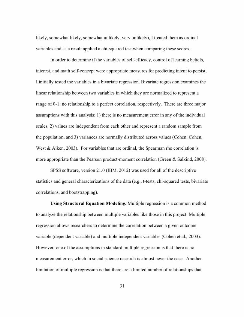
likely, somewhat likely, somewhat unlikely, very unlikely), I treated them as ordinal

variables and as a result applied a chi-squared test when comparing these scores.

In order to determine if the variables of self-efficacy, control of learning beliefs,

interest, and math self-concept were appropriate measures for predicting intent to persist,

I initially tested the variables in a bivariate regression. Bivariate regression examines the

linear relationship between two variables in which they are normalized to represent a

range of 0-1: no relationship to a perfect correlation, respectively. There are three major

assumptions with this analysis: 1) there is no measurement error in any of the individual

scales, 2) values are independent from each other and represent a random sample from

the population, and 3) variances are normally distributed across values (Cohen, Cohen,

West & Aiken, 2003). For variables that are ordinal, the Spearman rho correlation is

more appropriate than the Pearson product-moment correlation (Green & Salkind, 2008).

SPSS software, version 21.0 (IBM, 2012) was used for all of the descriptive

statistics and general characterizations of the data (e.g., t-tests, chi-squared tests, bivariate

correlations, and bootstrapping).

Using Structural Equation Modeling. Multiple regression is a common method

to analyze the relationship between multiple variables like those in this project. Multiple

regression allows researchers to determine the correlation between a given outcome

variable (dependent variable) and multiple independent variables (Cohen et al., 2003).

However, one of the assumptions in standard multiple regression is that there is no

measurement error, which in social science research is almost never the case. Another

limitation of multiple regression is that there are a limited number of relationships that

 

  32

can be specified between variables (Cohen et al., 2003). Structural Equation Modeling

(SEM) is more powerful than a standard multiple regression analysis because it allows

you to account for 1) measurement error which results in a more reliable measure of

regression and 2) multiple variables and the relations between those variables (Hoyle,

2012).

Structural Equation Modeling is a statistical approach to assessing a hypothesis

through a series of regression equations such that the relationships can be modeled

pictorially (Byrne, 2012). SEM is used to test a series of constructs through a

theoretically-proposed model using both continuous and discrete variables that allow

researchers to make predictions (Tabachnick & Fidell, 2001).

SEM analysis contains two unique models: 1) a measurement model, which tests

the relationship the data have to each other through a factor analysis; and 2) a structural

model that allows researchers to make theory-driven claims about the directional

relationship of the data (Kline, 2012), these directional claims are what allow for

predictions. So the measurement model tests if relationships exist between the proposed

constructs in the model and the structural model allows researchers to test if the proposed

directionality maps onto those constructs. Figure 4.1 introduces basic terminology

associated with the measurement model and figure 4.2 introduces the basic terminology

associated with the structural model.

 

  33

Figure 4.1. Illustration of the basic structure of a measurement model for SEM.

The latent factors are larger constructs (e.g., self-efficacy) that are informed by a

series of survey items (or other variables, such as test scores). Manifest (or observed)

variables are similar to latent construct, but they are represented by only one survey item

or by a directly observed measure. The arrows in the model that circle back onto a

variable or factor represent the measurement error for the individual items, or individual

variance that exists for a given factor. The single headed arrow from the individual items

to the constructs represent the factor loadings, which is the amount that each individual

item contributes to a given construct. The double-headed curved arrows between the

factors represents the shared variance, or correlation, between the different factors. A

manifest variable can be used in measurement models, but they are items that either have

only one item to represent a given construct or are a directly observed phenomena. The

weakness of a manifest is due to the lack of accounting for measurement error. However,

because manifest variables can have a shared variance with other factors it is important to

keep them at the factor level (Byrne, 2012; Hoyle, 2012).

I2

I1

I3

I4

I5

I6

MV

LF2

LF1

LF: Latent Factor MV: Manifest (or Observed) Variable

I: Item

 

  34

Figure 4.2. Illustration of the basic structure of a structural model for SEM.

In figure 4.2, the structural model has the same elements as the measurement

model, but there is now a directional path, which minimizes some of the correlations. As

a result, the structural model is nested within the measurement model. Nesting measures

a goodness-of-fit for the structural model. The goodness-of-fit does not assess the

directionality of the arrow, because that is theory-based rather than quantitatively

assessed (Byrne, 2012; Hoyle, 2012).

The proposed measurement and structural models for this research are presented

in Figure 4.3 and 4.4. The predictive variable in the structural model is intent to persist.

The latent variables are the Math Self-Concept (MSC), Self-Efficacy (SE), Control of

Learning Beliefs (CLB). Interest is a manifest variable and Classroom Pedagogy (RTOP)

is measured at the instructor level and is an observed variable, so will be treated

differently.

LF1

LF2

OV

LF: Latent Factor OV: Manifest (or Observed) Variable

 

  35

Figure 4.3. Proposed measurement model for this research project Figure 4.4. Proposed structural model for this research project

SE

CLB

MSC

Interest

Intent

SE: Self-efficacy CLB: Control of Learning Beliefs

Interest: Interest in Science

MSC: Math Self-Concept

Intent: Intent to Persist

CLB2

CLB3

CLB4

CLB1

SE16

SE37

SE24

SE58

MSC49

MSC57

MSC68

MSC23

MSC110

Interest

CLB

SE

Intent

MSC

SE: Self-efficacy CLB: Control of Learning Beliefs

Interest: Interest in Science

MSC: Math Self-Concept

Intent: Intent to

 

  36

The method for establishing a SEM with a solid foundation is based in many

decisions. Some of these decisions are with the data itself prior to analysis, how to best

analyze the data based on those initial decisions, what type of measurement model to use,

choosing when to modify the measurement model, and what the a priori structural model

should be. Figure 4.5 is a flow chart representing the decisions made for this research.

Some of these decisions were based on the software, all SEM analyses were done using

MPlus version 7.0 (Muthén & Muthén, 1998-2012).

 

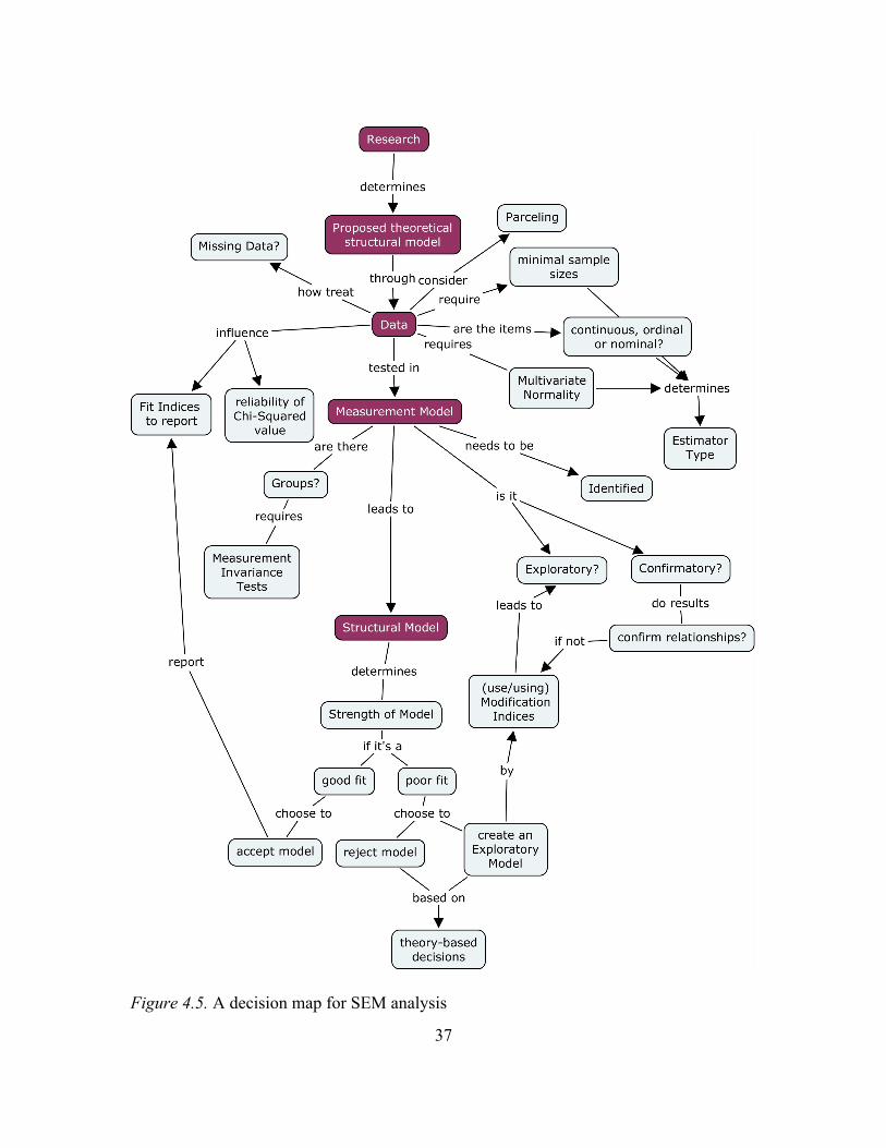
  37

Figure 4.5. A decision map for SEM analysis

 

  38

Data assumptions and decisions. Prior to any measurement or structural analysis

of the data, it is important for the researcher to be aware of the general characteristics of

the data. Measurement decisions are influenced by the normality or non-normality of the

data, the type of data collected, whether it be continuous variables, ordinal, or nominal

data, and how to best arrange the data for the structural model in order to make the most

parsimonious possible model.

Standard SEM analyses assume all data are multivariate normal. Data that are

heavily skewed by a shift in means and/or kurtotic by a shift in variance relationships can

impact the shape of the normal curve, which then impacts the accurate fit and

interpretation of the data (DeCarlo, 1997; Byrne, 2012). When data are not normally

distributed, there are ways to address this in MPlus software, however, it is important to

be aware of the degree of normality or non-normality of your data prior to analysis (Yuan

& Chan, 2005). In addition, ordinal or nominal data are generally not normally

distributed, and as such will influence the decisions made for the type of analysis. For

this project, I did an analysis of the normality of the data prior to any SEM analysis. In

addition, both the interest and intent variables were ordinal, and as a result, informed

some of my chosen methods to employ in MPlus.

SEM generally requires large sample sizes, 100 at a minimum, and many analyses

rely on more than 1,000, particularly as models become more complex (Tabachnick &

Fidell, 2001). When sample sizes are below 100, the models can become underpowered

and difficult to determine if the models are appropriate. The tests to determine if a model

is appropriate can become skewed and less reliable with smaller sample sizes (Bentler,

 

  39

1990). The data collected from the Spring 2013 CC sample (CCS) were lower than

predicted, and thus impacted the choice of estimator.

Data characteristics are important to know, because they influence the researchers

decisions with which estimator method to use. An estimation method informs how the

model is analyzed, based on how the data are treated. Which estimation method is

chosen can influence the quality of the model parameter estimates, their associated

standard error estimates, and the overall model fit statistics (Lei & Wu, 2012). An

estimator essentially determines how well the variance-covariance matrix fits to the

model of how it should ideally fit through an iterative process. The most common

estimator is the Maximum Likelihood estimator (ML), with the assumption that the data

are multivariate normally distributed and continuous data. If data are non-normal and/or

categorical (fewer than 5 categories; Rhemtulla et al., 2012), than the ML estimator is not

robust and can lead to inflated model fit likelihood and deflated standard error estimates

(Lei & Wu, 2012). More recently, estimators are available that adjust the ML estimator

for non-normal data known as an adjusted version of the Satorra-Bentler statistic (Lei &

Wu, 2012). For categorical data, the weighted least squares (WLS) takes a different

approach to estimating the model fit so that it relaxes the asymptotic assumption of the

data distribution, and as such can be much more robust to model fit, but relies on large

(>1,000) sample sizes (Lei & Wu, 2012). In general, ordinal data represent a larger

spectrum of a construct, but are represented by a smaller range (Byrne, 2012). For

example, interest in science is represented by an infinite range of possible responses from

strongly agree to strongly disagree, but in this research it was only represented by four

 

  40

options. The WLS estimator accounts for this theoretically larger range by calculating

thresholds and using those thresholds in the place of means in a continuous item

(Rhemtulla et al., 2012). More recent modifications have allowed for using a smaller

sample size with a modified version of the WLS, known as the Diagonally Weighted

Least Squares (DWLS) where it is computationally less intense (Lei & Wu, 2012).

Depending on which data I was using determined my estimator. When just analyzing

data from continuous variables, I used the MLR (ML estimator in MPlus available for

non-normally distributed continuous data). When analyzing the variables, both

continuous and ordinal (interest and intent), I used the DWLS estimator in MPlus,

WLSMV (Muthén & Muthén, 1998-2012).

Another concern is when data are missing in a larger data set. There are several

options for missing data, the most common approach in the social sciences has been

listwise deletion (Graham & Coffman, 2012). For example, students who did not

complete the semester (and/or the post-survey) were not included in an analysis because

we did not have their post-data. The problem with listwise deletion, particularly with

SEM, is that this method removes information that is not missing at random. Because, for

example, the reasons a student did not complete the course or the survey are probably due

to specific reasons. This non-randomness of removal potentially impacts the overall

score means, the strength of relationships between variables, and may result in estimation

bias and a loss of statistical power (Graham & Coffman, 2012). However, where there

are small sample sizes, listwise deletion may be the best option since other variables rely

on a large data set to draw inferences about the missing data (Little, 2013). Multiple

 

  41

imputation (MI) is another approach to handling missing data, where it pulls from the

data that does exist to estimate a plausible value. However, it is still based on the idea

that the data are missing at random, rather than not-at-random (Graham & Coffman,

2012). In addition, it requires a large dataset from which to pull other possible variables

(Little, 2013), if large percentages of a small data set are missing, it may rely too heavily

on the data that are present, in addition MI can be problematic for ordinal variables

(Graham & Coffman, 2012). Lastly, Full-Information Maximum Likelihood (FIML) is

the most robust way of treating missing data in which there are multiple steps to impute

the missing data pulling from the full dataset (Graham & Coffman, 2012). When dealing

with missing data in this project, most of the analysis was based only on post-results, so

there was no need for handling missing data as the subjects of focus were those students

completing the course, and there were no missing data from the Spring 2013 (CCS and

R1S) post-survey responses. However, in cases within the larger 2008-2013 GARNET

dataset (CCF and R1F) where there were missing data, I employed the MPlus default for

handling missing data, which is a form of FIML for the SEM measurement and structural

analyses.

When creating a theoretical model for SEM analysis, there are decisions that need

to be made about how individual items measure larger latent constructs. A researcher can

accept the default created by the original designers of survey items. Alternatively,

parceling is an option if there are similar items that may co-vary. Parceling is the process

of bundling individual items and taking their average score as a manifest or observed

variable that informs a larger latent construct. The benefit of parceling is that it

 

  42

maximizes the reliability, or the common-to-unique factor variance, increases the

tendency toward multivariate normality, and creates a more parsimonious model (Little,

Cunningham, Shahar & Widaman, 2002). The disadvantage is that it can increase the

possibility of Type-I error by capitalizing on chance (Marsh et al., 2013). However,

when the larger latent construct is of interest rather than individual items, and when

parceling is considered carefully with theoretical considerations, it can greatly strengthen

the overall model fit (Little et al., 2002; Little, Rhemtulla, Gibson & Schoemann, 2013).

I chose to parcel the self-efficacy (from eight items to four) and math self-concept items

(from ten items to five).

Measurement model decisions. Once the data have been analyzed and established

into a measurement model, the next steps in decision making include how to assure that

your model is appropriately identified, how to handle comparison of models across

groups, and whether to employ a confirmatory or exploratory factor analysis with the

data.

The identification of a given model is based on the number of correlations within

the model as compared to the number of parameters, or the number of factor loadings and

number of factor correlations. The number of correlations minus the number of

parameters represents the degrees of freedom. In order to generate a meaningful

measurement model, it must be a minimum of a just-identified model, where the number

of parameters is equal to the number of correlations, and the degrees of freedom are zero.

In other words, the number of variances and co-variances are equal to the things in the

model a researcher would like to estimate. Much more meaningful comparisons occur

 

  43

when models are over-identified, or there are leftover degrees of freedom. Models are

not possible when they are under-identified. In addition, you must have more than two

latent constructs predicting one outcome in the final structural model in order to be more

than just-identified (Byrne, 2012; Hoyle, 2012).

When comparing different groups, one of the most critical parts of the

measurement model analysis is to establish multiple group invariance or equivalency in

response to the items across these groups. Groups are defined by the researcher, and ones

that represent different populations that may be expected to respond to survey items

differently, such as individuals from different countries, different age groups of students,

or students attending different types of institutions. Because these groups are

independent of one another, I need to establish that the data are not invariant across the

groups (Byrne, 2012). Jöreskog (1971) was the first to describe this process, by which he

argued that if groups are invariant, they can be pooled for analysis. By examining the

variances and co-variances across the groups, a researcher can determine if participants in

different groups are responding to questions in a similar manner. This would indicate that

both groups are interpreting the questions in the same way, thus making the items

invariant to the groups. The traditional way to measure invariance is to test at three

levels of increasing restriction to the model across the groups where configural tests the

parameters across groups, which are then followed by a weak invariance, testing the

measurement equivalence and the strong invariance, testing the structural equivalence. In

this research, I was particularly interested if I could compare how R1 students responded

to the survey items as compared to CC students. As a result, an invariance test was

 

  44

required. The challenge for this project was that by combining manifest and latent

variables due to the properties of the data, the traditional measures of group invariance

were not available to be tested (Byrne, 2012). As a result, my test for invariance was less

conservative than the more traditional configural test with follow-ups. I chose to employ

a test that compared groups invariance through an omnibus goodness-of-fit test, which

essentially equates to the configural test, but does not allow for follow-up tests (Byrne,

2008). However, measurement and structural equivalence were tested across the latent

variables (SE, CLB, & MSC).

The last decision prior to doing the factor analysis of a measurement model is

determining if it will be a Confirmatory Factor Analysis (CFA) or an Exploratory Factor

Analysis (EFA). Both factor analyses measure the variance and covariances between

different measures or indicators. In a CFA, these variances are restricted to a

parsimonious, theoretically-driven idea of what should and should not correlate. Whereas

an EFA is a data-driven decision making process, which allows the researcher to free up

all the variables and create a more parsimonious model based on the data itself (Brown &

Moore, 2012). In SEM analysis, the CFA-EFA process can be somewhat fluid, where

starting with a CFA of pre-defined theoretical constructs can change into an EFA by

looking at the modification indices in the output from the analysis. At the measurement

level, choosing a CFA or EFA is largely based on the goals of the researcher. If I were

testing the individual items and whether they mapped onto a given construct, an EFA

would be the logical process. The modification indices are what would be the source of

information from which choices can be made about better fitting models based on

 

  45

variables that share variance with multiple latent constructs and/or other items (Byrne,

2012). I chose not to employ an EFA approach for my measurement models since the

self-efficacy, control of learning beliefs, and math self-concept subscales are already well

supported within the literature, so I used a CFA in which I examined the relationships

between the constructs. In fact, using modification indices at the measurement model as

an EFA could lead to a bad model that would be based on data rather than prior work

(Byrne, 2012).

Structural model decisions. The last step in SEM analysis is the actual structural

analysis. In this portion of modeling, a model is generated that predicts an outcome,

which is directionally based. The analysis measures the loading on the predicted

outcome by the different predicted measures based on the CFA/EFA measurement model.

The final decisions for the structural model are how to best compare the best-fitting

models, which are based on fit indices.

In SEM, the most traditionally reported fit index is the chi-squared, goodness-of-

fit test. A chi-squared test determines how well your more parsimonious model fits

relative to a completely unrestrained model with all parameters varying with one another

(Bentler, 1990). Chi-squared tests are highly subject to poor measurement fit when the

models have large sample sizes or are not multivariate normally distributed. As a result,

most models in the social sciences will be underestimated applying a chi-squared test

because they tend to either violate the multivariate normality assumption or contain large

sample sizes (Yu, 2002; West, Taylor & Wu, 2012). As a result, different fit indices

(both goodness and badness of fit) have emerged. There are absolute fit indices, such as

 

  46

Standardized Root Mean square Residual (SRMR), which measures the parameters

relative to the error variances relative to a weight matrix, and has been standardized to a

0-1 value, in which the closer to 0 the better (a badness of fit). It is sensitive to N, but

does not penalize someone for a more complex model or greater number of parameters

(West et al., 2012). For non-normally distributed data, particularly with ordinal data, the

WRMR has the most consistent power with acceptable type I error across all sample sizes

(Yu, 2002). An example of comparative fit is the Comparative Fit Index (CFI), which is

robust to non-normality and small sample sizes, but it may be overly conservative with an

N less than 200 (Bentler, 1990). It is generally encouraged that researchers report the chi-

squared and several selected model fit indices to illustrate the overall fit of a model.

Table 4.2 represents the indices I used for this project and the generally accepted cut-off

values. It should be noted however, that rigorous cut-off values are less appropriate when

data are non-normally distributed (Yuan & Chan, 2005), so any criteria for cut-offs with a

non-normally distributed and small data sets must be measured with caution.

Table 4.2 Fit indices reported in this research with cut-off values and affordances and constraints of each. Fit Index Cutoff Type of Fit Reason for including

Chi-Square < 0.05 Goodness Standard practice to report, unreliable with smaller sample sizesa

RMSEA < 0.06 Badness Standard practice to report, tends to over reject with smaller sample sizesa,b

CFI > 0.95-.96 Goodness Least sensitive to N and robust to non-normalitya, b, c

WRMR < 0.95-1.0 Badness Appropriate with ordinal data (low type-I error for non-normally distributed data)b

SRMR < 0.08 Badness Appropriate for continuous data, sensitive to N, but not to model complexitya

a West et al., 2012, b Yu, 2002 c Bentler, 1990

 

  47

Ultimately, the fit indices are what are used to make decisions about how well a

structural model fits the data. If a model does not fit the data, the researcher can decide

to stop and end the research, or decide to do a post-hoc analysis using modification

indices, similar to that mentioned in the measurement model of a CFA analysis moving

into a an EFA. The same caution serves the researcher here, such that decisions that are

still theoretically sound rather than simply relying on the data to inform these decisions.

While I did not employ an EFA during the measurement model phase, I did choose to

employ post-hoc analyses of structural models which resulted in some EFA based on the

reality of the actual data rather than the idealized theoretically proposed model.

However, all decisions were checked to assure they still met with the original intent of

the proposed model.

Finally, when different estimators are used, the traditionally reported chi-squared

tests may not be as reliable of a comparison. In this project, with the use of ordinal

variables, interest and intent to persist, a different estimator was used. As a result, the

chi-squared test comparison required a “difftest” result, in which a hypothesis test of

nested models was used to obtain a reliable chi-squared value (Muthén & Muthén, 1998-

2012). When comparing the two groups (R1 and CC), I tested the chi-squared tests as a

modification of the standard test Δchi-squared = [chi-squared1 –chi-squared2], Δdf = [df1-

df2]. Traditionally, in SEM, degrees of freedom are determined by the number of

parameters in the model, however, in this case, since both models had the same number

of parameters, it was not possible to obtain a traditional measure of Δdf. As a result, I

modified the Δdf test to be = [n1-n2] (a more traditional measure of degrees of freedom in

 

  48

regression analysis; Cohen et al., 2003). Cutoff criterion for this test were p > 0.05 for

ΔΧ2 and < 0.01 for ΔCFI (Cheung & Rensvold, 2002), because I was testing the

hypothesis that there was not a significant difference between these populations. When

testing for invariance across the continuous variables only (SE, CLB, & MSC), the

estimator used was MLR in MPlus, which is treated for non-normally distributed data.

As a result, Χ2 for each MLR model is reported, but are not reliable to be used for

goodness-of-fit comparisons.

Using Structural Equation Modeling to Compare and Contrast Populations.

In order to determine if there was a significantly positive relationship between geology

expectancy, interest and students intent to persist in another geology class, I conducted a

SEM analysis for both the R1F and CCF population. When analyzing a model with a

second order model, like expectancy as represented by sub-latent constructs of CLB &

SE, a minimum of three constructs must be used in order to assure that the model is not

just identified (Byrne, 2012). As a result, in this initial analysis, I treated CLB and SE as

their own latent constructs rather than as a second order expectancy construct. Further

analyses determined if expectancy was an appropriate assumption for these SEM models.

Ideally, the most appropriate analysis for determining the role of instructor in

student’s intent to persist should be multi-level modeling (MLV) in which instructor

RTOP score is on one level and the student data are on a different level (Byrne, 2012).

Some argue that a minimum of 100 instructors would be required to do a MLV analysis

(Hox & Maas, 2001), but others have argued that stability and reliability can still be

obtained with numbers closer to 50 (Cheung & Au, 2005). Even at 50, there were not

 

  49

enough instructor RTOP scores for any institution from the entire GARNET population

to be able to do this analysis. As a result, I treated the different RTOP groups as ordinal

variables as student-centered, transitional, and traditional (high to low) as defined by

Budd et al., 2013. In order to test this variable, I separated students from different

classrooms into different models comparing the high RTOP category with the medium

RTOP category for the community college population and all RTOP categories for the R1

population. I only created two categories for the community college population because

there was only one classroom that fit the low category. I ran each of the tests as an

omnibus test similar to how I tested for invariance across groups. If these populations

were different, they would fail the invariance test.

Lastly, I examined the role that math self-concept played in these models.

Initially, I ran a CFA model with the continuous items only (SE, CLB, and MSC) to

determine if a 2nd order factor of overall geology expectancy was a more appropriate fit

for the data in either population. Based on these findings, I ran a final structural model

using SE, CLB, MSC, and Interest in predicting intent to persist (Intent) for both

populations (figure 4.4).

After all models were analyzed, I then tested for mediation and moderation.

Baron and Kenny (1986) proposed a method to test for mediation and moderation of an

outcome illustrated in figure 4.6 and 4.7. In mediation, if a variable, such as interest were

removed from the model, and another variable, such as self-efficacy were to predict

intent to persist, the original variable (e.g., interest) may serve as a mediator. A further

test for this mediation is if those same variables were significantly related in a basic

 

  50

regression. So if self-efficacy were to predict intent to persist when interest was removed,

but only co-varied with interest when interest was in the model, then it would be likely

that interest served as a mediator.

Figure 4.6. Adapted model of mediation from Baron & Kenny (1986)

In contrast, moderation influences a model in a much more subtle way. Figure

4.7 illustrates how moderation might influence variables within this model.

Figure 4.7. Adapted model of moderation from Baron & Kenny (1986)

In this case, if both variables self-efficacy and interest predicted intent to persist,

but there was an interaction that influenced the strength or even the direction of the

predictor, it may indicate a moderating relationship. Put another way, a moderating

variable can impact the strength of an association either through dampening or enhancing

an effect (Little, 2013).

Intent

Interest

Self-Efficacy

Self-Efficacy

Interest

Interest x Self-Efficacy

Intent

 

  51

Results

Characterizing the data

In order to compare the R1S and CCS sample responses, chi-squared tests

compared the interest and intent to persist variables. Results are reported in table 5.1.

Table 5.1 Results from Chi-squared tests comparing R1S and CCS to the R1F and CCF. Variable Institution Χ2 df p Cramér’s V

Interest R1 54.11 4 < 0.001 0.15 CC 8.33 4 0.08 0.13

Intent R1 24.53 4 < 0.001 0.10 CC 3.61 4 0.46 0.08

Note: R1S and CCS represent the Spring 2013 GARNET dataset, R1F and CCF represent the full GARNET population

Table 5.1 illustrates that while there are statistically significantly differences

between R1F and R1S, they are not meaningful differences based on the Cramér’s V

effect size. Effect sizes less than 0.30 are considered to be small and less than 0.10 are

inconsequential (Cohen, 1969). The sample sizes of the full GARNET data set for these

analyses were 2,339 and 454 for the R1F and CCF populations, respectively. After

bootstrapping the larger population to calculate a t-value and standard deviation for an

equivalent size population, t-test comparisons revealed minor differences in R1F and R1S

and no difference between CCF and CCS. Results reported in table 5.2 illustrate that

while there were statistically significant differences between R1F and R1S, the differences

were small as the effect size from Cohen’s d illustrates.

 

  52

Table 5.2. Results from t-test comparing R1S and CCS with bootstrapped population of R1F and CCF. Institution Sample set N M sd t df p d

R1 Bootstrap 167 60.91 13.21 3.24 165 0.001 -0.24 Spring 13 166 63.96 12.13

CC Bootstrap 79 63.38 13.22 -0.27 77 0.79 -0.02 Spring 13 78 63.09 15.06 Note: R1S and CCS represent the Spring 2013 GARNET sample, R1F and CCF represent the full GARNET population

Item reliability tests determined if the math self-concept items could be

appropriately used with this population. These resulted in highly reliable Cronbach alpha

values (α = 0.941; αR1S = 0.946; αCCS = 0.930) which were better than or the same

reliability as the initially reported results of α = 0.93 (Marsh, 1984).

Analysis of variance components of the CCS and R1S demonstrated that between

83.3% and 97.1% of the variability in the expectancy scores was attributable to within

student variability, as opposed to between institution/classrooms, and that between 93.1%

and 95.1% of the variability in the math self-concept scores was attributable to within

student variability, as opposed to between instructors. In addition, analysis of variance

components demonstrated that between 98.6% and 99.4% of the variability in the interest

scores was attributable to within student variability, as opposed to between instructor and

that between 90.9% and 94.4% of the variability in intent to persist was attributable to

within student variability, as opposed to between instructor/institution. All of this

suggests that multilevel modeling would not provide much benefit. In addition, as

reported in Budd et al., 2013, many of these introductory geology classrooms are similar

in what is happening in these classrooms.

 

  53

In examining the missing data for the CCS and R1S sample, the range of students

who completed both pre and post tests were 43%-100%. Other than the lowest

completion percent (27), this range was well within the general range of responses within

the entire GARNET data set for 2012-2013 collection year (29-94%, average 71%

response rate). One classroom’s data were thrown out from the CCS dataset due to the

large number of missing post-responses (73%) and the procedure for reminding faculty to

administer the post-survey was not followed. As such it seemed to represent an outlier of

extreme missing data and would likely not be representative of the larger data set, and

could even possibly skew the results. In addition, all of the items analyzed for the SEM

analyses were from post-semester responses only, as a result, this cross-sectional dataset

prevented the need to handle a large degree of missing data. In SEM analysis, there were

between 2 and 3 missing data patterns for the R1F population and between 1 and 2

missing data patterns for the CCF population.

In examining the descriptive statistics for characterizing the general scores from

student responses to the categories of expectancy, math self-concept, interest and intent to

persist, there was a small to moderate negative skew to a number of the items. Table 5.3

provides a characterization of the data. The non-normality of these data were not extreme

(Rhemtulla et al., 2012), but were considered when analyzing the data.

Table 5.3. Descriptive statistics of the four major subscales used for this research at each institution. Subscale item Institution type Mean s.d. Skewness Kurtosis

Interest R1 3.08 0.962 -0.625 -0.783 CC 2.99 0.845 -0.903 0.647

 

  54

Intent R1 2.46 1.094 0.150 -1.282 CC 2.37 0.982 0.200 -0.932

Expectancy R1 63.96 12.13 -0.298 -0.475 CC 62.92 15.00 -0.627 -0.255

Math Self-concept R1 50.24 18.38 -0.200 -0.694 CC 45.08 19.07 -0.101 -1.042

Note: These data are from the CCS and R1S sample

In comparing the samples of R1S to CCS for measurement invariance when using

SEM, I conducted an omnibus test comparing chi-squared values and CFI values. Table

5.4 reports the values between these two samples.

Table 5.4 Measurement invariance omnibus test all variables. Population N Χ2 a df CFI R1 166 28.19 4 0.94 CC 78 25.34 4 0.94 Note: These tests are based on CFA that included self-efficacy, control of learning beliefs, math self-concept, interest and intent to persist variables a Χ2 is a report of the difftest result from MPlus software due to use of categorical and continuous variables.

Chi-squared difference test (Χ2R1- Χ2

CC, NR1-NCC) revealed that ΔΧ2 = 2.85, ΔN

(substituting for df) = 88, p = 1.0. The ΔCFI values = -0.006, which is within the

accepted cutoff of 0.01 (Cheung & Rensvold, 2002). These results allowed me to make

comparisons across institutional populations in a meaningful and consistent way.

In testing the continuous variables only, for a full invariance test, I tested for

configural, weak and strong invariance. The results are reported in table 5.5. The test for

invariance holds across all levels, so the sample of R1S and CCS responses can be

compared across groups. While the nested p value for the strong invariance test is less

 

  55

than the 0.05 cutoff, because it is still within the CFI < 0.01, which is a more reliable

measure for small sample sizes, I found this to be an acceptable measure of invariance.

Table 5.5 Measurement invariance tests for continuous items Test Χ2 df nested p CFI ΔCFI Configural 200.78 124 0.96 Weak 214.34 134 0.19 0.96 0.002 Strong 233.15 144 0.04 0.95 0.005 Note: Each test is nested within the previous. Characterizing the population

In order to characterize and compare R1S sample to the CCS sample, a series of

chi-squared analyses tested demographic differences. The first test comparing the

proportion of sex represented in the sample (gender on the survey) revealed that there

was no significant difference between the two groups (Pearson Χ2sex(1, N = 245) = 1.76, p

= 0.18, Φ = 0.09). There were 88 men and 79 women in the R1S data set and 34 and 44

men and women, respectively, in the CCS dataset. In comparing the proportion of

different ages, races, and choice of major, there were significant differences between

these two samples (Pearson Χ2age(3, N = 245) = 29.55, p < 0.001, Cramérs V = 0.35;

Pearson Χ2race-all(8, N = 245) = 44.04, p < 0.001; Pearson Χ2

race-condensed(1, N = 245) =

30.49, p <0.001, Φ = 0.35; Pearson Χ2major(3, N = 245) = 18.54, p <0.001, Cramérs V =

0.28). Results from these comparisons are visually presented as comparisons in figures

5.1-5.3.

Students attending CC were older than those at a R1. The proportion of students

over the age of 22 in a CC classroom was 0.33 relative to 0.11 for a R1 student. The

 

  56

probability of a student over the age of 22 attending a CC as 3.0 times as likely than at a

R1.

Figure 5.1. Students ages represented at both institutions reported as percentages. CCS students are generally older than their R1S counterparts in this study.

Students in an introductory geology classroom at a R1 were more likely (0.43) to

be a declared a STEM major (Earth Science or any other STEM) than at a CC (0.16).

The probability of a STEM major in a R1 introductory geology classroom was 2.7 times

more likely than at a CC. In addition, CC students were less certain about their major

overall. The proportion of undecided majors at a CC was 0.5 versus 0.29 for R1 students

in introductory geology classrooms. The probability of an undeclared major at a CC was

1.7 times more likely than at a R1.

 

  57

Figure 5.2. Students at the community college are more likely to be undeclared or non-stem relative to their R1 counterparts. R1 students are more likely to be declared STEM majors.

Because race had several occurrences of fewer than 5 cases, I chose to combine

the non-white race into one category for a more accurate chi-square test. In that analysis,

the proportion of nonwhite students at R1’s versus CC’s was 0.14 and 0.46, respectively.

The probability of a non-white student attending a CC was 3.3 more times as likely

(0.46/0.14) than at a R1.

 

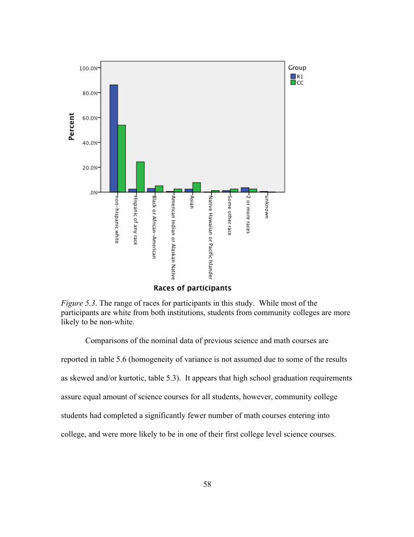
  58

Figure 5.3. The range of races for participants in this study. While most of the participants are white from both institutions, students from community colleges are more likely to be non-white.

Comparisons of the nominal data of previous science and math courses are

reported in table 5.6 (homogeneity of variance is not assumed due to some of the results

as skewed and/or kurtotic, table 5.3). It appears that high school graduation requirements

assure equal amount of science courses for all students, however, community college

students had completed a significantly fewer number of math courses entering into

college, and were more likely to be in one of their first college level science courses.

 

  59

Table 5.6 Comparison of previous science and math courses taken by students enrolled at different institutions. Courses Institution Mean s.d. t p df d College science

R1 1.59 1.33 3.89 0.0001 176.5 0.59 CC 0.95 1.13 High School math

R1 3.64 0.80 2.68 0.008 158.5 0.43 CC 3.36 0.76 High school science

R1 3.44 1.28 0.55 0.59 130.4 0.096 CC 3.33 1.53

College math R1 1.65 1.24 -0.50 0.62 150.6 0.081 CC 1.74 1.34 Note: College science and High school math are statistically significant when applying Holm’s Bonferonni test (Holm, 1979).

Comparing reasons students enrolled in their introductory geology courses, the

overwhelming reason for enrollment for all students was to satisfy a general education

requirement, which agrees with previous findings (Gilbert et al., 2012). Figure 5.4

illustrates the responses to each of the different categories. Students were able to select

more than one response, so the sums are greater than the total N. Results are reported in

table 5.7. The proportion of students who were more likely to enroll as a general

education requirement at a R1 versus a CC was 0.70 versus 0.84, respectively. As a

result, the probability of a CC student enrolling in an introductory geology class due to a

general education requirement was 1.21 times more likely than a R1 student. In addition,

the probability that students who anticipated that the class would be easier (than other

general education requirements) at a R1 than a CC was 1.5 times more likely. However,

the proportion of students at a R1 who were enrolling because they were more interested

was higher at a R1 than at a CC (0.39 versus 0.24, respectively). As a result, the

probability of a student interested in the topic was 1.6 times more likely than in a CC

 

  60

classroom. Both of these results have implications for student motivation and incoming

expectancies and valuing of the course. A R1 student had a higher probability of

capitalizing on social capital by entering in the course based on a recommendation (0.35

versus 0.19 for a CC student). The probability of a R1 student receiving a

recommendation for taking the course was 1.8 times as likely than for a CC student.

Lastly, it should be noted that students may have misinterpreted the option of “required

for a major/minor,” when examining the percent responses to choosing the course for a

general education requirement and required for a major/minor, the total percent adds to

more than 100% for both the R1 and CC response sets. Ideally, these two options should

be an either/or situation, so it should not add to more than 100% responses. It is possible

that some students were interpreting a requirement for graduation (general education

requirements) as part of the requirement for their major.

Figure 5.4. Reasons students selected to enroll in the course, most students are enrolled for general education requirements, but also have other reasons for enrolling.

0  

10  

20  

30  

40  

50  

60  

70  

80  

90  

Percent  response  

Reasons  for  Enrolling  

R1  

CC  

 

  61

Table 5.7 Reasons for students enrolling in the course. Reason for enrolling

Institutiona N proportion Χ2 df p ϕ

General Education

R1 116 0.70 5.77 1 0.02 0.15 CC 66 0.85 Required for Major/Minor

R1 68 0.41 0.001 1 0.98 -0.002 CC 32 0.41

Prior Interest R1 64 0.39 5.05 1 0.03 -0.14 CC 19 0.24

Recommendation R1 58 0.35 6.39 1 0.01 -0.16 CC 15 0.19

Easier R1 51 0.31 2.87 1 0.09 -0.11 CC 16 0.21 Human-Env Interactions

R1 42 0.15 3.11 1 0.08 -0.11 CC 12 0.15

Instructor R1 22 0.13 0.03 1 0.88 0.01 CC 11 0.14

Other R1 16 0.10 1.46 1 0.23 -0.08 CC 4 0.05

Do not know R1 4 0.02 1.92 1 0.17 -0.09 CC 0 0.00 Note: Question and stem options are in Appendix A, students could select multiple options. aN for R1 = 165, CC = 78.

In comparing the student responses from different institutions for expectancy,

math self-concept, interest and intent to persist there were significant differences between

the CCS and R1S sample (all the results assume non homogeneity of variance based on

results from table 5.3). An independent t-test was used to determine if there were

differences between R1S and CCS responses for expectancy and math self-concept scores.

There was no difference between the two samples for expectancy scores (texpectancy = 0.53

(126.01), p = 0.60, d = 0.10), but there was a statistically significant difference in math

self-concept between these two samples (tmath self-concept = 2.55 (142.50), p = 0.01, d =

0.43) with a moderate effect size. A chi-squared test was used to determine if there were

 

  62

differences between the two samples for interest and intent to persist scores. There was

no difference in intent to persist (Χ2intent = 3.81 (df = 3, N = 244), p = 0.28, Cramér’s V =

0.13, but there was a statistically significant difference in interest scores between the R1S

and CCS samples (Χ2interest = 22.79 (df =3, N = 244), p < 0.001, Cramér’s V = 0.31) with a

moderate effect size. Based on means and standard deviations for these populations

(table 5.3), for both interest and math self-concept, the R1 sample had higher scores

relative to their CC counterparts.

In order to compare the different items proposed in the structural equation model,

a bivariate regression analysis was run using Spearman rho for ordinal values and

Pearson product-moment correlation for values that only involved continuous variables.

Based on the previous analysis of normality, the assumptions of these analyses were

violated, however, it is a first pass at determining relationships. Results are reported in

table 5.8. While intent to persist was not directly related to math self-concept in either

population, it was related to other subscales, and as such merits a more detailed

examination of how these different scales work together to predict intent to persist.

Table 5.8 Bivariate correlations among items used for SEM analysis with R1a and CCb students (in bold)

Intent to Persist Interest

Control of Learning Beliefs (CLB)

Self-Efficacy (SE)

Math Self-Concept (MSC)

Intent --- 0.54*** 0.18 0.34** 0.04 Interest 0.40*** --- 0.18 0.36** 0.08 CLB 0.19* 0.25** --- 0.71*** 0.22 SE 0.28*** 0.48** 0.64*** --- 0.32** MSC 0.04 0.20* 0.10 0.27** ---

 

  63

a N = 166 (R1S), b N = 78 (CCS) * = p < 0.05, ** = p < 0.01, *** = p < 0.001

SEM Analysis Prior to SEM analysis, I initially ran the variables from the CCS and R1S samples

in a measurement model CFA to examine the relationships of the items and chose to

parcel the self-efficacy items and the math self-concept items. I chose theoretically

logical pairings, and for those that didn’t have an obvious pairing, I chose them based on

the modification indices, and paired the low with the high (Little et al., 2012). Table 5.9

illustrates the pairing and indicates which were parceled based on content and which

where parceled based on modification indices.

Table 5.9

Parceling of subscale items for SEM analysis

Subscale Statements Parceled item

Self-Efficacy

I believe I will receive an excellent grade in this class 1

6 a I expect to do well in this class I’m certain I can understand the most difficult material presented in readings for this course 2

4 a I’m confident I can understand the most complex material presented by the instructor in this course I’m confident I can understand the basic concepts taught in this course 3 b

7 I’m certain I can master the skills being taught in this class I’m confident I can do an excellent job on the assignments and test in this course 5 b

8 Considering the difficulty of this course, the teacher, and my skills, I think I will do well in this course.

Math Self-Concept

I find that mathematical problems interesting and challenging 1

10 a I have never been very excited about math I have hesitated to take courses that involve 2

 

  64

math 3 a I have generally done better in math courses than other courses Math makes me feel inadequate 4

9 a At school, my friends always come to me for help in math I am quite good at math 5

7 a I have always done well in math I have trouble understanding anything that is based upon math 6

8 b I never do well on tests that require math a parceled based on theoretical similarities, b parceled based on modification indices

In comparing the relationship between SE, CLB, interest and students intent to

persist in another geology class, I conducted a SEM using the WLSMV estimator.

Because this initial analysis did not contain math self-concept as an item, I used the CCF

and R1F populations. Figures 5.5 and 5.6 illustrate the models from this analysis for CCF

and R1F. In all models, variance, co-variances and pathways are all values that are

significant at p < 0.001 unless otherwise noted. The initial structural analysis revealed

that Χ2difftest = 205.43, df = 2, p = 0.00; N = 536; RMSEA = 0.09 (0.08-0.10); CFI = 0.88;

WRMR = 0.71. Since these values generally did not meet the cutoff criterion (table 4.2),

a post hoc analysis revealed a shared error variance between two variables in control of

learning beliefs increased the overall fit of the model, Χ2difftest = 253.75, df = 3, p = 0.00;

N = 536; RMSEA = 0.06 (0.04-0.07); CFI = 0.95; WRMR = 0.50. Since this model was

right at the cutoff criteria, I proceeded to share error variance with two items in the self-

efficacy subscale, which was the next recommended change in the modification indices.

After this last test, the final model produced a strong fit, Χ2difftest = 206.60, df =2, p =

0.00; N = 536; RMSEA = 0.04 (0.02-0.06); CFI = 0.98; WRMR = 0.39.

 

  65

Figure 5.5. Structural model for CCF responses predicting intent to persist based on self-efficacy (SE), control of learning beliefs (CLB) and interest. Note: Post hoc analysis additional co-variances are indicated by dashed lines. New values are bolded. The gray arrow on intent indicates a fixed construct variance of 1.0, all construct variables were fixed at 1.0. n.s. = not significant, p values in brackets.

The first model for the R1F population also did not meet the cutoff criterion,

Χ2difftest = 988.33, df =2, p = 0.00; N = 2505; RMSEA = 0.09 (0.08-0.09); CFI = 0.89;

WRMR = 1.35. As a result, I also did a post-hoc analysis for this model, however, in

order for the models to be comparable, after examining the modification indices, I chose

to co-vary the same subscales without creating a secondary model. The final model

SE

Interest

CLB

Intent 1*  

SE16   SE24   SE37   SE58  

.62  

.79   .84   .92   .89  .76   .84   .92   .86  

C1   C2   C3   C4  

.39  

.72   .61   .81  .58  

.72   .58   .80   .55  

.86  

.45  

.34  

.90  

.46  

.34  

.12n.s.  [.32]  

.45  

.11n.s.  [.37]  

.11n.s.  [.53]  

.45  

.12n.s.  [.49]  

 

  66

produced a strong fit, Χ2difftest = 999.56, df =2, p = 0.00; N = 2505; RMSEA = 0.04 (0.03-

0.04); CFI = 0.98; WRMR = 0.58.

Figure 5.6. Structural model for R1F responses predicting intent to persist based on self-efficacy (SE), control of learning beliefs (CLB) and interest. Note: Post hoc analysis additional co-variances are indicated by dashed lines. New values are bolded. n.s. = not significant, p value provided in brackets, ** = p < 0.01.

Both of these models, once adjusted for shared error variance within self-efficacy

and control of learning belief items, predicted intent. Control of learning beliefs did not

predict intent to persist in either of these models. Whereas, self-efficacy was a predictor

.80   .86   .93   .99  .76   .86   .93   .86  

SE  

Interest  

CLB  

Intent   1*  

.76  .61   .85  

.57  

.76   .58   .85   .54  

.51  

.39  

.83   .86  

.51  

.40  

.14**  

.41  

-­‐.01n.s.  [.85]    

.16**  

.40  

-­‐.03n.s.  [.57]  

C1   C2   C3   C4  

.33  

SE16   SE24   SE37   SE58  

.57  

 

  67

of intent for the R1 population only. Interest was the strongest predictor for success with

both populations, predicting at least 40% of the variance in intent to persist.

In comparing instructor pedagogy, I compared high vs. medium RTOP categories

for the CCF population and all categories for the R1F population in omnibus tests similar

to an invariance test. The results for these analyses are reported in table 5.10. These

results indicate that there was likely a difference between the RTOP classrooms as the

ΔΧ2 values did not indicate a difference, but the CFI comparisons do. Comparing the CC

classrooms, ΔΧ2 = 17.2, ΔN (substituting for df) = 71, p =1.0, but ΔCFI = -0.08, which

was not within the accepted cutoff value of 0.01. Because the ΔΧ2 is less reliable, I

looked to the ΔCFI for a more reliable measure of comparison across classrooms when

there was disagreement. As a result, it appears that there was a difference between these

two populations. Similar comparisons existed at the R1F classroom comparisons, where

ΔΧ2(high-middle) = -77.65, ΔN = -314, p =1.0, and ΔCFI = 0.08; ΔΧ2

(middle-low) = 111.84, ΔN

= 252, p =1.0, and ΔCFI = -0.07; and ΔΧ2(high-low) = 34.19, ΔN = -62, p =0.998, and ΔCFI

= 0.01. These results indicated that there were differences between the classrooms,

although the differences between the high and the low were minimal, since they were

right at the CFI cutoff value of 0.01.

Table 5.10 Results of CFA comparisons between different RTOP classrooms. Institution RTOP Χ2 a df N CFI

R1 High 469.95 3 686 0.94 Middle 547.60 3 1000 0.86 Low 435.76 3 748 0.93

CC High 153.57 3 286 0.85

 

  68

Middle 136.37 3 215 0.93 Note: Separation of categories is based on categories established by Budd et al., 2013 where a low RTOP represents a traditional classroom (RTOP < 30), middle RTOP represents a transitional classroom (RTOP 30-50), and high RTOP represents a student-centered classroom (RTOP > 50). a Results are reported as the chi-squared difftest from MPlus due to the WLSMV estimator used for categorical variables.

When comparing the SEM models for these different classrooms, a nested chi-

squared comparison revealed that, again, there were differences in these populations.

However, none of the originally proposed models was a strong predictor of intent to

persist. None of the models were within the accepted cut off values, as revealed in table

5.11. Post-hoc analysis revealed that when the same items in control in learning beliefs

and self-efficacy co-varied as from the first models (figures 5.5 and 5.6), these models

became significant (figures 5.7-5.11). Figures 5.7 and 5.8 represent the CCF population,

and figures 5.9-5.11, the R1F population.

Table 5.11 SEM regression results for different RTOP ranked classrooms in both original analyses and post-hoc (ph) results. Institution RTOP Χ2 a df N RMSEA CFI WRMR

R1

High 357.19 3 686 0.08 0.92 0.71 High ph 282.11 2 686 0.03 0.99 0.39 Middle 481.55 3 1000 0.10 0.84 1.04 Middle ph 390.71 2 1000 0.05 0.97 0.52 Low 382.09 3 748 0.08 0.91 0.71 Low ph 306.42 2 748 0.03 0.99 0.37

CC

High 127.56 3 286 0.10 0.83 0.65 High ph 100.57 2 286 0.06 0.95 0.39 Middle 115.30 3 215 0.07 0.92 0.42 Middle ph 89.75 2 215 0.04 0.98 0.30

a Results are reported as the chi-squared difftest from MPlus due to the WLSMV estimator used for categorical variables.

 

  69

Figure 5.7. SEM for high RTOP CCF classrooms. Note: Post hoc analysis additional co-variances are indicated by dashed lines. New values are bolded. While not indicated on the diagram, construct variance was fixed to 1.0 for all construct variables. n.s. = not significant, p values in brackets, * = p < 0.5.

.80   .84   .92   .90  .77   .84   .92   .86  

SE16   SE24   SE37   SE58  

.63  

SE  

Interest  

CLB  

Intent  

.27*  

.39  

.01n.s..  [.95]  

.30n.s.  [.08]  

.38  

.04n.s.  [.77]  

.51  

.37  

.82  

.52  

.38  

.86  

.75   .58   .82   .53  .75   .53   .82   .49  

C1   C2   C3   C4  

.43  

 

  70

Figure 5.8. SEM for middle scoring RTOP CCF classrooms. Note: Post hoc analysis additional co-variances are indicated by dashed lines. New values are bolded. n.s. = not significant, p values in brackets.

For both models at the community college (figures 5.7 & 5.8), interest continued

to be the only predictor of intent to persist. However the % of variance that interest

predicted in intent to persist varied between these two models, where the middle scoring

RTOP classrooms had a higher percent explained than the high RTOP classrooms.

SE  

Interest  

CLB  

Intent  

-­‐0.34n.s.  [.20]  

.53  

.47n.s.  [.09]  

.92n.s.  [.11]  

-­‐.81n.s.  [.17]  

.57  

.40  

.33  

.92  

.41  

.34  

.96  

.79   .84   .91   .89  .75   .84   .91  

.86  

SE16   SE24   SE37   SE58  

.61  

.69   .68   .79   .67  .68   .65   .78   .64  

C1   C2   C3   C4  

.35  

 

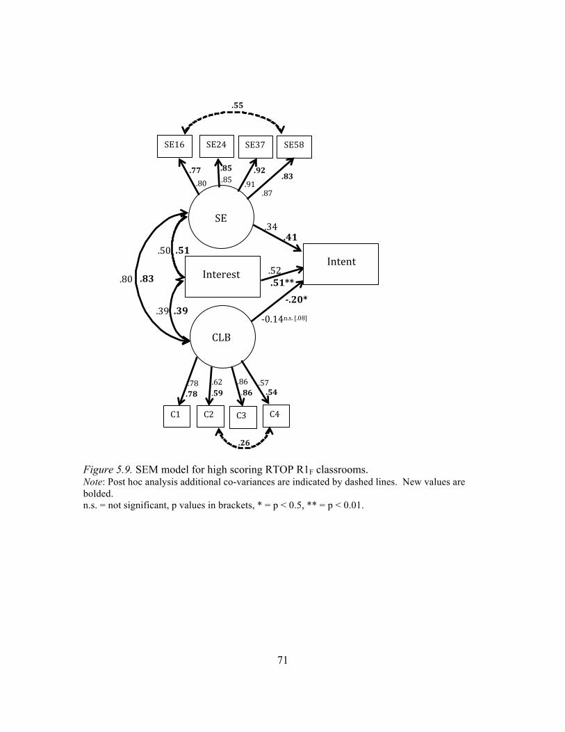
  71

Figure 5.9. SEM model for high scoring RTOP R1F classrooms. Note: Post hoc analysis additional co-variances are indicated by dashed lines. New values are bolded. n.s. = not significant, p values in brackets, * = p < 0.5, ** = p < 0.01.

SE  

Interest  

CLB  

Intent  

.34  

.52  

-­‐0.14n.s.  [.08]  

-­‐.20*  

.41  

.51**  

.80   .85   .91  .87  

.77   .85   .92  .83  

SE16   SE24   SE37   SE58  

.55  

.50  

.39  

.80  

.39  

.51  

.83  

C1   C2   C3   C4  

.78   .86   .57  .62  .78   .86   .54  .59  

.26  

 

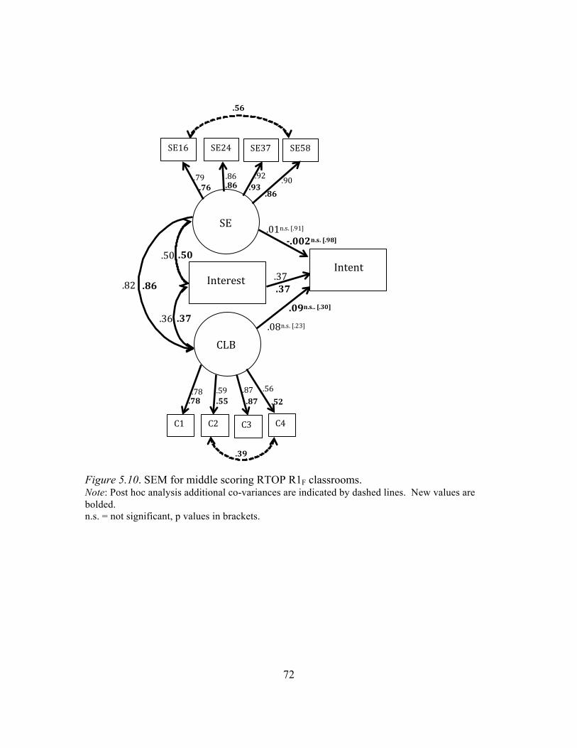
  72

Figure 5.10. SEM for middle scoring RTOP R1F classrooms. Note: Post hoc analysis additional co-variances are indicated by dashed lines. New values are bolded. n.s. = not significant, p values in brackets.

SE  

Interest  

CLB  

Intent  

.01n.s.  [.91]  

.37  

.08n.s.  [.23]  .09n.s..  [.30]  

-­‐.002n.s.  [.98]  

.37  

.50  

.36  

.82  

.50  

.37  

.86  

.79   .86   .92   .90  .76   .86   .93  

.86  

SE16   SE24   SE37   SE58  

.56  

.78   .59   .87   .56  .78   .55   .87   .52  

C1   C2   C3   C4  

.39  

 

  73

Figure 5.11. SEM for low scoring RTOP R1F classrooms. Note: Post hoc analysis additional co-variances are indicated by dashed lines. New values are bolded. n.s. = not significant, p values in brackets.

In each of these models, interest consistently predicted intent to persist. However,

at R1 institutions, in high RTOP scoring classrooms only, self-efficacy also directly

predicted intent to persist and control of learning beliefs negatively predicted intent to

persist (figure 5.7). Other than high RTOP classrooms in R1 institutions, as the classroom

became more teacher-centered, interest became a stronger predictor of intent to persist,

SE  

Interest  

CLB  

Intent  .53  

.43  

.86  

.54  

.44  

.89  

.10n.s.  [.31]  

.41  

.01n.s.  [.96]  

.12n.s.  [.38]  

.41  

-­‐.01n.s.  [.92]  

.80   .86   .94   .92  .77   .86   .94   .89  

SE16   SE24   SE37   SE58  

.60  

.74   .63   .83   .57  .74   .60   .83   .54  

C1   C2   C3   C4  

.32  

 

  74

which would indicate that students would need to have a strong interest if they were not

engaged in the classroom to want to persist. The one exception, high RTOP classrooms

at the R1 (figure 5.7), had many different variables that contributed, which lessons the

impact that interest alone would need to predict.

In order to determine if CLB, SE, and MSC should be loaded as a second order

factor of geology expectancy, I ran a CFA with just the continuous variables on their own

in order to compare to the second order factor model. Results for R1S and CCS are below

in table 5.12 and in figures 5.12 and 5.13. When running the 2nd order factor model, the

self-efficacy factor loaded with a negative residual variance, which resulted in an

impossible model. This held consistent even in post-hoc analyses. As a result, there was

no evidence that a second order factor model would strengthen the results of the model.

As a result, in the final model, they were treated as separate latent constructs. However,

it should be noted that self-efficacy and control of learning beliefs consistently co-vary to

a very high degree (ranges from 83-96% in all models analyzed), and as a result, the

previous assumption for testing t-tests of self-efficacy and control of learning beliefs as a

greater expectancy construct was appropriate, it is just not possible to test a SEM with

only two latent constructs on a single second order factor, as the model would be just

identified which would not change the interpretation of individual models (Byrne, 2012).

However, the CFA model illustrated a strong fit for these variables.

 

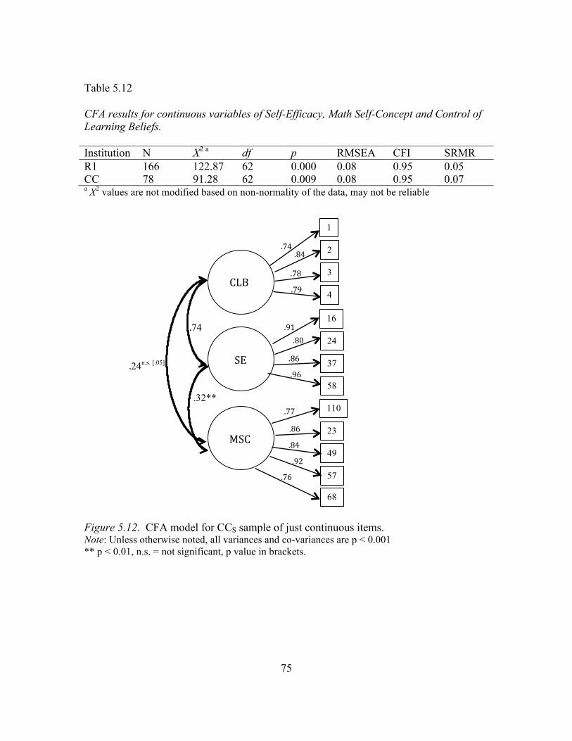
  75

Table 5.12 CFA results for continuous variables of Self-Efficacy, Math Self-Concept and Control of Learning Beliefs. Institution N Χ2 a df p RMSEA CFI SRMR R1 166 122.87 62 0.000 0.08 0.95 0.05 CC 78 91.28 62 0.009 0.08 0.95 0.07 a Χ2 values are not modified based on non-normality of the data, may not be reliable Figure 5.12. CFA model for CCS sample of just continuous items. Note: Unless otherwise noted, all variances and co-variances are p < 0.001 ** p < 0.01, n.s. = not significant, p value in brackets.

CLB  

1

2

3

4

.74  .84  

.78  

.79  

SE  

16

24

37

58

.91  .80  

.86  

.96  

MSC  

110

23

49

57

68

.77  

.86  

.84  

.92  

.76  

.24n.s. [.05]  

.32**

.74  

 

  76

Figure 5.13. CFA model for R1S sample of just continuous items. Note: Unless otherwise noted, all variances and co-variances are p < 0.001 ** = p < 0.01, n.s. = not significant, p value in brackets.

In comparing the final proposed model, I did a SEM that included math self-

concept. Results are reported in table 5.13 and in figures 5.14 and 5.15. Neither of the

original models were statistically significant. As a result, a post-hoc, EFA analysis was

done to determine the best-fit model for the data in each of these populations. The CCS

model did not have any possible modifications, it was already as complete of a model as

presented, however, a post-hoc analysis of R1S was possible. The post hoc analysis of

this model revealed that the best alteration for the data were if the control of learning

beliefs shared variance with one item in math self-concept, both of which were items that

CLB  

1

2

3

4

.65  .68  

.88  

.58  

SE  

16

24

37

58

.83  .75  

.89  

.89  

MSC  

110

23

49

57

68

.86  

.92  

.87  

.89  

.79  

.10n.s.[.19]  

.28**

.79  

 

  77

include a control of learning aspect to the statements (“I have trouble understanding

anything that is based upon math” and “I never do well on tests that require math”).

Because the math self-concept items were only collected in the spring semester, it is

possible that the CCS model is simply underpowered, as it is right at the CFI cut off

value, and the RMSEA and WRMR values are within acceptable range. Because SEM

analyses are subject to variation based on sample size and normality, it is ultimately up to

the researcher to determine the acceptability of a model (Byrne, 2012), as such, I think

that the CCS model with the math self-concept variable included is likely a relatively

good representation of the student’s intent to persist at community colleges. In comparing

the two original models of R1S and CCS, the ΔCFI = -0.02, and the ΔΧ2 = 5.9, ΔN = 88, p

= 1.0, which would indicate that these models are not invariant, which indicates that how

math self-concept plays a role in these models differs.

Table 5.13 SEM regression results for the full model of Interest, Self-Efficacy, Math Self-Concept and Control of Learning Beliefs in predicting intent to persist. Institution N Χ2 a df p RMSEA CFI WRMR R1 166 17.91 3 0.001 0.05 0.93 0.56 R1-post hoc 166 14.89 3 0.001 0.03 0.97 0.46 CC 78 12.01 3 0.007 0.04 0.95 0.41 a chi-squared test results from “difftest” in MPlus software calculation

 

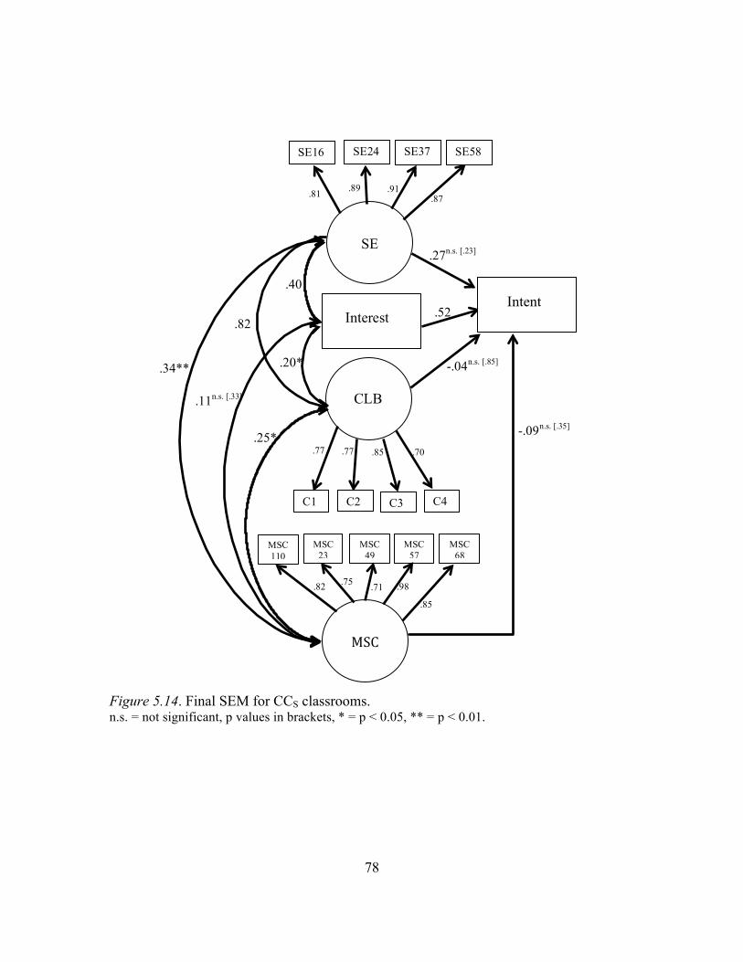
  78

Figure 5.14. Final SEM for CCS classrooms. n.s. = not significant, p values in brackets, * = p < 0.05, ** = p < 0.01.

SE

Interest  

CLB  

Intent

MSC  

SE16 SE24 SE37 SE58

.81 .89 .91 .87

C1 C2 C3 C4

.77 .77 .85 .70

.27n.s. [.23]

-.04n.s. [.85]

-.09n.s. [.35]

.52

.40

.20*

.25*

.82

.11n.s. [.33]

.34**

MSC 110

MSC 23

MSC 49

MSC 57

MSC 68

.82 .75 .71 .98

.85

 

  79

Figure 5.15. Final SEM for R1S classrooms. Note: Post hoc analysis additional shared variance is indicated by dashed lines. New values are bolded. n.s. = not significant, p values in brackets, * = p < 0.05.

These models reveal that while MSC does not predict intent to persist in either

model, it did co-vary with self-efficacy and interest with the R1 population and with SE

SE16 SE24 SE37 SE58

.80 .74 .93 .88

.79 .74 .93 .88

C1 C2 C3 C4

.66 .63 .90 .58

.66 .64 .91 .58

SE

Interest  

CLB  

Intent

MSC  

.18

.14n.s. [.39]

.15n.s. [.38]

.02n.s. [.92]

-.08n.s. [.37]

.01n.s. [.95]

-.08n.s. [.36]

.37

.37

MSC 110

MSC 23

MSC 49

MSC 57

MSC 68

.88 .83 .83 .87

.90

.91 .88 .86 .90 .77

.51

.37

.13n.s. [.11]

.78

.19*

.30

.51

.37

.13n.s. [.08]

.77

.17*

.26

 

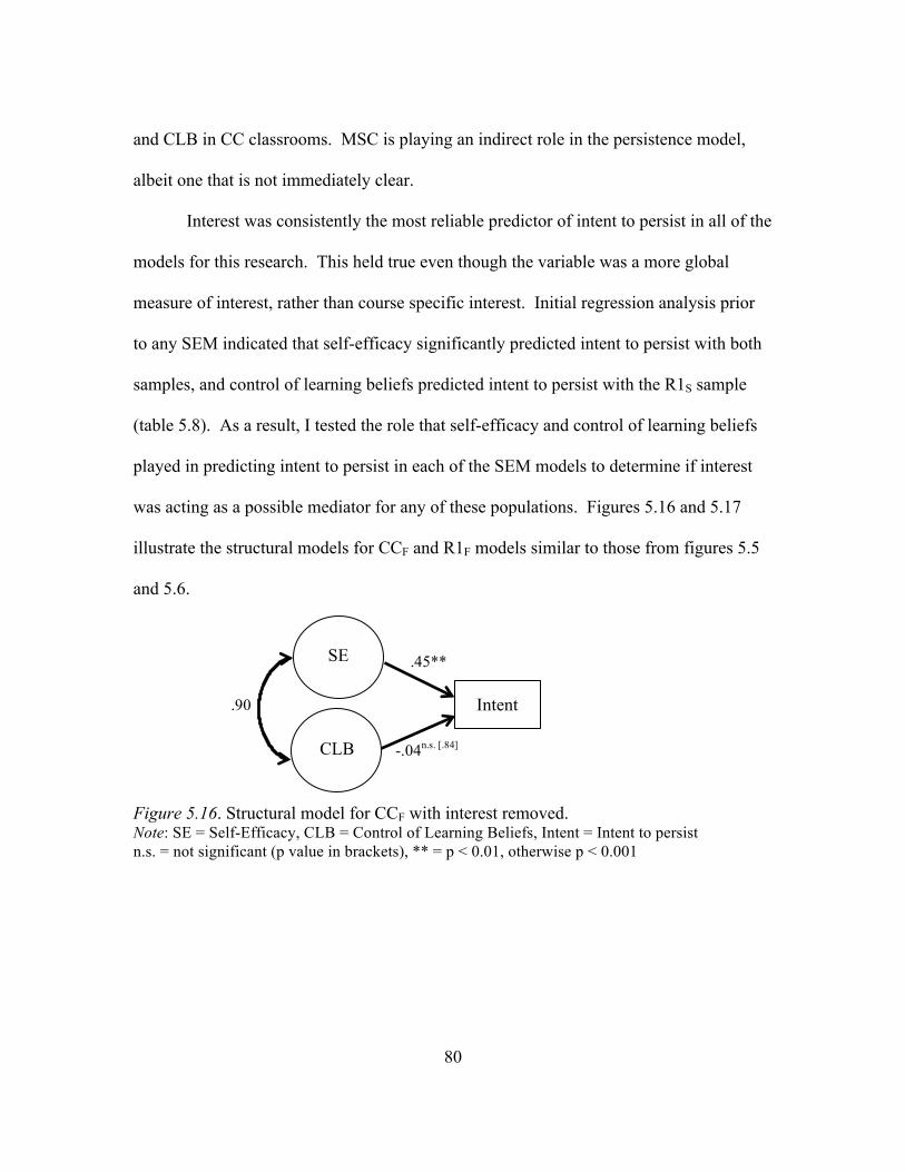
  80

and CLB in CC classrooms. MSC is playing an indirect role in the persistence model,

albeit one that is not immediately clear.

Interest was consistently the most reliable predictor of intent to persist in all of the

models for this research. This held true even though the variable was a more global

measure of interest, rather than course specific interest. Initial regression analysis prior

to any SEM indicated that self-efficacy significantly predicted intent to persist with both

samples, and control of learning beliefs predicted intent to persist with the R1S sample

(table 5.8). As a result, I tested the role that self-efficacy and control of learning beliefs

played in predicting intent to persist in each of the SEM models to determine if interest

was acting as a possible mediator for any of these populations. Figures 5.16 and 5.17

illustrate the structural models for CCF and R1F models similar to those from figures 5.5

and 5.6.

Figure 5.16. Structural model for CCF with interest removed. Note: SE = Self-Efficacy, CLB = Control of Learning Beliefs, Intent = Intent to persist n.s. = not significant (p value in brackets), ** = p < 0.01, otherwise p < 0.001

.45**

-.04n.s. [.84]

.90 Intent

SE

CLB

 

  81

Figure 5.17. Structural model for R1F with interest removed. Note: SE = Self-Efficacy, CLB = Control of Learning Beliefs, Intent = Intent to persist n.s. = not significant (p value in brackets), otherwise p < 0.001

These figures illustrate that when interest was removed, self-efficacy replaced

interest as the predicting variable for intent to persist, in both cases, it predicted almost

the same amount as interest did in the original models (table 5.14). Both of these models

were built from the final post-hoc models where self-efficacy and control of learning

beliefs shared error variance. The fit indices for both of these models still indicates a

good fit, where the CCF model was Χ2difftest = 139.53, df = 1, p = 0.000, RMSEA = 0.04,

CFI = 0.98, WRMR = 0.34 and the R1F model was Χ2difftest = 681.60, df = 1, p = 0.000,

RMSEA = 0.04, CFI = 0.98, WRMR = 0.61.

Table 5.14

SEM results when interest variable was removed from original models

The story becomes a bit more complex when the role of instructor is considered as

a function of RTOP. Re-examining these models when interest is removed reveals a

Institution % interest predicted in original model

What predicts when interest was removed

% predicted

CCF 45% Self-Efficacy 45% R1F 40% Self-Efficacy 44%

.44

-.11n.s. [.07]

.86 Intent

SE

CLB

 

  82

slightly more nuanced result, however, in general, self-efficacy tends to replace the role

of interest (figures 5.18 and 5.19 for CCF structural models and 5.20-5.22 for R1F

structural models).

Figure 5.18. Structural model for CCF with interest removed in high RTOP classrooms Note: SE = Self-Efficacy, CLB = Control of Learning Beliefs, Intent = Intent to persist n.s. = not significant (p value in brackets), otherwise p < 0.001

Figure 5.19. Structural model for CCF with interest removed in middle RTOP classrooms Note: SE = Self-Efficacy, CLB = Control of Learning Beliefs, Intent = Intent to persist n.s. = not significant (p value in brackets), otherwise p < 0.001

Figure 5.20. Structural model for R1F with interest removed in high RTOP classrooms Note: SE = Self-Efficacy, CLB = Control of Learning Beliefs, Intent = Intent to persist n.s. = not significant (p value in brackets), * = p < 0.05, otherwise p < 0.001

.70

-.25*

.83 Intent

SE

CLB

-.21n.s. [.70]

.54n.s. [.34]

.96 Intent

SE

CLB

.57

-.08ns [.64]

.86 Intent

SE

CLB

 

  83

Figure 5.21. Structural model for R1F with interest removed in middle RTOP classrooms Note: SE = Self-Efficacy, CLB = Control of Learning Beliefs, Intent = Intent to persist n.s. = not significant (p value in brackets), ** = p < 0.01, otherwise p < 0.001

Figure 5.22. Structural model for R1F with interest removed in low RTOP classrooms Note: SE = Self-Efficacy, CLB = Control of Learning Beliefs, Intent = Intent to persist n.s. = not significant (p value in brackets), ** p < 0.01, otherwise p < 0.001

In this case, the high scoring RTOP CCF model illustrates that self-efficacy is an

even stronger predictor for intent to persist when interest is removed, whereas with the

middle RTOP CCF classroom, there was nothing that significantly predicted interest.

With the R1F classrooms, the predictors are more consistent with previous results, Self-

efficacy and negative control of learning beliefs continues to predict interest, with an

increased weight to each individual variable, and self-efficacy replaces predicting interest

in the R1F middle and low RTOP classrooms with fairly consistent levels of replaced %

variance explained (table 5.15).

Intent

SE

CLB

.42**

-.10n.s. [.47]

.89

.26**

.002n.s. [.98]

.86 Intent

SE

CLB

 

  84

Table 5.15

SEM results when interest was removed from RTOP classroom models

As with the other interest-removed models, the fit indices indicated a strong fit for

each of these models (table 5.16).

Table 5.16 SEM regression results for different RTOP ranked classrooms where interest was removed. Institution RTOP Χ2 a df N RMSEA CFI WRMR

R1F High 189.55 1 686 0.04 0.98 0.38 Middle 271.64 1 1000 0.05 0.97 0.50 Low 208.76 1 748 0.04 0.98 0.40

CCF High 65.27 1 286 0.06 0.95 0.36 Middle 62.58 1 215 0.03 0.99 0.25

Note: all fit indices were based on post-hoc models from original models prior to interest removal where self-efficacy and control of learning beliefs shared error variance. a Results are reported as the chi-squared difftest from MPlus due to the WLSMV estimator used for categorical variables.

In the final model, when interest was removed, self-efficacy again becomes the

consistent predictor that replaces interest in predicting intent to persist. Figures 5.23 and

5.24 illustrate these new structural models for CCS and R1S, respectively. Table 5.17

compares the original model predictor of interest to the new models.

RTOP scale Institution % Interest predicted

What predicts intent after interest is removed % predicted

High CCF 38 Self-Efficacy 57 Middle CCF 37 Nothing --

High R1F 51 Self-Efficacy, Control of Learning

70, -25 (respectively)

Middle R1F 37 Self-Efficacy 26 Low R1F 41 Self-Efficacy 42

 

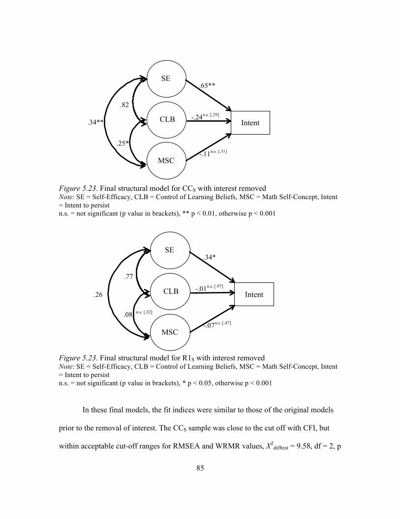
  85

Figure 5.23. Final structural model for CCS with interest removed Note: SE = Self-Efficacy, CLB = Control of Learning Beliefs, MSC = Math Self-Concept, Intent = Intent to persist n.s. = not significant (p value in brackets), ** p < 0.01, otherwise p < 0.001

Figure 5.23. Final structural model for R1S with interest removed Note: SE = Self-Efficacy, CLB = Control of Learning Beliefs, MSC = Math Self-Concept, Intent = Intent to persist n.s. = not significant (p value in brackets), * p < 0.05, otherwise p < 0.001

In these final models, the fit indices were similar to those of the original models

prior to the removal of interest. The CCS sample was close to the cut off with CFI, but

within acceptable cut-off ranges for RMSEA and WRMR values, Χ2difftest = 9.58, df = 2, p

Intent

SE

CLB

MSC

.65**

-.24n.s. [.29]

.82

-.11n.s. [.31] .25*

.34**

Intent

SE

CLB

MSC

.34*

-.01n.s. [.97]

.77

-.07n.s. [.47] .08 n.s. [.32]

.26

 

  86

= 0.008, RMSEA = 0.04, CFI = 0.94, WRMR = 0.42. The post-hoc interest-removed

model for the R1S sample was a good fit, Χ2difftest = 10.98, df = 2, p = 0.004, RMSEA =

0.03, CFI = 0.98, WRMR = 0.46.

Table 5.17

SEM results when interest was removed from the final model

All of the interest-removed models indicate a relationship between self-efficacy

and interest. In some cases, self-efficacy replaces the role of interest in an almost exact

amount of variance. In other cases, there is more or less variance explained by self-

efficacy than was by interest alone. As a result, this may be an indication of possible

moderating relationships taking place within these models.

Discussion

The results from this research reveal several possible implications for community

college students, and students in introductory geology classrooms in general. In

particular, are the impacts that an instructor may play a role in student interest and the

possible implications for student persistence in the geosciences.

In this research, I was examining the role that self-efficacy, control of learning

beliefs, interest and in some cases, math self-concept played in predicting a student’s

intent to persist in taking another geology course. For this study, self-efficacy, as

Institution % Interest predicted

What predicts intent once interest is removed % predicted

CC 52 Self-Efficacy 65 R1 37 Self-Efficacy 34

 

  87

measured on the MSLQ as a student’s self-evaluation of how well they expect to do in

their geology course. Control of learning beliefs also measured by the MSLQ as a

measure of a student’s perception of how well they are in control of their grade and their

ability to learn the geology content. Because these measures were from the last third of

the semester, it is likely to be a more accurate gauge of these measures than their

incoming scores because they had been able to calibrate their expectations to the actual

classroom experience (Zusho et al., 2003). The combination of self-efficacy and control

of learning beliefs was operationalized as expectancy within portions of this research

(Appendix B). Math self-concept was measured from the SDQ III as a measure of a

more global aspect of how students feel about their ability to do math and their

preference for doing so (Appendix C). Interest and intent to persist were both measured

with individual items from the GARNET demographic survey (Appendix A).

Differences between Community College and University Students

There were measureable differences between community college students (CCS) and

university students (R1S) both demographically and affectively. Students enrolled in

introductory geology classes at the community college were more diverse, older, had

fewer STEM majors (including the geosciences), more undeclared majors, had less

incoming interest, but also fewer expectations of the course as an easy course. In

addition, CCS students had fewer prior math courses and were more likely to be in their

first college-level science course. Many of these findings support national trends in

which CC students are more diverse and older, and may lack the prior experiences to be

 

  88

able to gauge what to expect from a college level course (NCES, 2001; NSF, 2009;

AACC, 2012).

In addition to demographic differences, there were also measureable differences

between CCS and R1S students with regards to math self-concept and interest. R1S

students were leaving geology classrooms with a higher math self-concept and a greater

interest in science. These findings were consistent with the demographic measures. If

R1S students have had more math courses prior to entering the introductory science

courses, it is likely their math self-concept will be higher. In addition, since more R1S

students entered the course with interest, it is likely that there will be more leaving the

course interested. However, these differences have not been documented in the literature

prior to this research.

Lastly I hypothesized that there would also be differences between CC and R1

students with regards to intent to persist and expectancy for success in the course, and

these differences were not found to be true. These results counter previous findings of

students in other STEM disciplines at the community college. For example, student self-

efficacy in introductory engineering classrooms were found to be lower in community

college classrooms than in R1 institutions (Baker, Wood, Corkins & Krause, 2012). If

interest and math self-concept were lower with community college students, but intent to

persist was not, this may indicate that even with lowered interest, CC students may be

willing to consider taking another geology course.

With both samples, the negative skew in intent to persist indicated that there were

fewer numbers of students reporting continuing on to take another geology class. This

 

  89

was an unfortunate result, because our greatest chance of capturing students is not in the

first course they take, but in subsequent courses. Wilson’s recent report on geoscience

graduates indicated that the second year of coursework was the highest likelihood of

when students decide to become geology majors (Wilson, 2013). This would mean that

the chances of capturing geology majors in the introductory geology courses is low, but if

they choose to take more geology courses, their likelihood of becoming a major

increases.

Role of Expectancy and Interest in Predicting Intent to Persist

There was a significantly positive relationship between expectancy, interest and

intent to persist with both CCF and R1F populations. In the CCF population, interest was

the only direct predictor, predicting 45% of the variance in intent to persist. Both self-

efficacy and control of learning beliefs (expectancy) played an indirect role in this model

as they significantly co-varied with interest, but were not direct predictors of intent to

persist. Within the R1F population, both interest and self-efficacy predicted intent to

persist, explaining 56% of the variance. Again, while control of learning beliefs did not

directly predict intent, it did significantly co-vary with both interest and self-efficacy.

Interest was measured as a global measure of interest, rather than specifically

identifying a type of situational or individual interest as described by Hidi and Renninger

(2006) or even as a subject specific measure. And yet, in this research, it was the most

consistent predictor of intent. It predicted 45% of the variance in intent to persist with

the CCF population and 40% in the R1F population. This finding is consistent with what

Harackiewicz and colleagues (2000) found with introductory psychology students.

 

  90

Students who were most likely to take another psychology course were those who had the

greatest interest.

Role of the Instructor

In this research, the Reformed Teaching Observation Protocol (RTOP) was used

to measure the instructor pedagogy as classified by the degree to which they created an

environment that allowed for students to interact with each other as much as with the

instructor (Appendix D). Due to limitations in the number of classrooms involved in this

project, the RTOP was broken down into three different categories based on the degree of

student interactivity. From this process, it became clear that that the degree of student

interactivity in the classroom played a role in predicting student intent to persist,

however, the relationships were nuanced and complex. Table 6.1 breaks down the

relationships with the different classrooms.

Table 6.1

Predictors of intent to persist in different RTOP classrooms

Institution RTOP ranking a Direct predictors of intent % predicting intent

CCF High Interest 38 Medium Interest 57

R1F High Interest, Self-Efficacy,

Control of Learning Beliefs 51, 41, -20 (respectively)

Medium Interest 37 Low Interest 41

a Rankings based on recommendations by Budd et al., 2013.

In all of these models, other than the high RTOP classrooms at the R1F, the results

were consistent with the previous models where interest was the only direct predictor of

intent to persist. Ignoring the high RTOP R1F classroom, a general trend of increasing

level of interest as a predictor of intent to persist becomes apparent. This trend may

 

  91

indicate that instructors were supporting students in other ways not measured in this

model that helped to predict intent to persist in classrooms where there was greater

interaction between both classmates and the instructor. Classrooms that were more

instructor-centered, students needed to maintain their interest in order to persist in taking

another geology course, as a result, interest played a larger role in predicting intent to

persist.

In the high RTOP R1F classroom, the relationship became much more complex.

Self-efficacy and interest both positively predicted intent to persist and control of

learning beliefs negatively predicted intent to persist. This indicates that students who

had a high self-efficacy were almost as likely to persist as those with high interest. The

fact that a decline in control of learning beliefs positively predicted intent to persist is a

bit concerning. This indicated that as students had less control over their own learning,

the more likely they were to take another geology course. This may have some negative

consequences for long term persistence with majors. If students think they are simply

good at doing geology, rather than thinking that they have worked hard to become

proficient, when faced with future challenges, could result in a decline in persistence.

With all of these models, there was a clear indication that instructor played a role

in a student’s intent to persist. This is in contrast to the initial calculation that there was

greater variance between students within a classroom than between different classrooms.

However, because classrooms within a given RTOP range were taught in similar ways

(Budd et al., 2013), this discrepancy may be as a result of the commonalities within

certain RTOP ranges.

 

  92

While the findings may not reveal what other factors in the classroom may

contribute to supporting students intent to persist, previous work has illustrated other

benefits from more student-centered classrooms. Students are more likely to learn in

student-centered classrooms, this has been demonstrated in work like that of Hake’s

seminal work in Physics college classrooms (Hake, 1998). In addition, Zusho et al.,

(2003) demonstrated that in general, student self-efficacy declined through the course of

the semester in other introductory science courses, but students with a high self-efficacy,

were more likely to perform better in the course. Our recent GARNET findings have

confirmed these same results of increased learning gains and high self-efficacy predicting

performance with introductory geoscience courses. In addition, we have found that

student-centered classrooms were more likely to minimize the need for expectancy (as

measured by self-efficacy and control of learning beliefs) to predict performance and

learning (van der Hoeven Kraft et al., 2013). Highly student-centered classrooms help

support student learning, support their self-efficacy, and based on my research may also

minimize the role that interest is needed to persist.

Role of Math Self-Concept in Expectancy for Success

Expectancy has been measured in this research as combining self-efficacy and

control of learning beliefs, however in SEM analysis, creating a second-order factor of

expectancy from two sub-constructs does not contribute to the interpretation of the

model. This is because at a local level within the model, expectancy would be just-

identified and as such, limits model interpretations (Byrne, 2012). However, I

hypothesized that the expectancy factor would include math self-concept for the R1S

 

  93

population and not for the CCS population, as I predicted that math self-concept would

play a greater role on it’s own with the CCS population due to their higher need for

developmental courses. However, when I added math self-concept to self-efficacy and

control of learning beliefs as contributors to a larger second order construct of expectancy

the model fell apart for both R1S and CCS populations. As a result, math self-concept

was a more powerful predictor as it’s own variable than it was as a larger expectancy

construct. With that being said, these variables as separate latent constructs still created a

strong measurement model where math self-concept and self-efficacy shared variance,

but control of learning beliefs only shared variance with self-efficacy.

These findings are consistent that self-efficacy and self-concept measure similar

constructs, but are distinctly different measures. Bong and Clark (1999) argued that self-

concept is a reflective way of viewing ones self and self-efficacy is a predictive future

path. In my research, the consistent high level of covariance of self-efficacy and control

of learning beliefs supports previous work that expectancy is an appropriate larger

second-order construct encompassing self-efficacy and control of learning beliefs

(Hilpert et al., 2013).

Role of Math Self Concept in Predicting Intent to Persist

By adding math self-concept to the predictive model, I had hypothesized that not

only would it increase the strength of predicting the model in predicting intent to persist,

but that it would also be different in the pathways of how it predicted between R1S and

CCS populations. Math self-concept did not play a significant role in predicting intent to

persist in either model. However, the models that included math self-concept were

 

  94

significantly different from one another in how math self-concept interacted with other

variables in the model. The complexities of interactions within each model indicated that

the more parsimonious model without math self-concept may be missing some important

variables, and that there are other possible variables that should be considered in

predicting persistence. Table 6.2 illustrates the ways that the models vary with the newly

added variable of math self-concept.

Table 6.2

Relationships in SEM models with Math Self-Concept

Institution % of intent predicted by interest

What co-varies with math self-concept

CCS 52 Control of Learning Beliefs, Self-Efficacy

R1S 37 Interest, Self-Efficacy

In the CCS model, a high degree of interest was required when predicting intent to

persist with the math self-concept variable added into the model. In addition, math self-

concept co-varied with self-efficacy and control of learning beliefs, but not with interest.

In contrast, the R1S model indicated that interest played less of a role in predicting intent

to persist and math self-concept co-varied with interest and self-efficacy. So while both

models were predictive of intent to persist, and math self-concept did not play a role in

directly predicting intent to persist, how it interacted with the different variables did

differ between different types of institutions. In particular, when interest was removed

from the model, self-efficacy predicted a much higher amount of variance than interest

did. These results suggest that math self-concept may have played a moderating role in

 

  95

interest in science and self-efficacy for the community college population, but not for the

R1 population.

The relationships between math self-concept, self-efficacy and interest are not

clear based on these models, however, a math self-concept role of moderation has

implications for the likelihood of community college student persistence in the

geosciences. In particular, if students at a community college lack the cultural capital of

access to prior math courses, it may increase the challenges students face in overcoming

the hurdle of persisting. This is not to say that CC students have a lowered likelihood of

persisting because they are CC students, rather the students who are more likely to attend

a CC are those who lack the background content which may impact their responses to

math self-concept. Previous research has indicated that math self-efficacy was mediated

by math self-concept (Miller & Pajares, 1994). Because the measures in this research

were geology self-efficacy and math self-concept, there may not be as direct of a

relationship, but these latent interactions may be influencing the outcome of interest on

intent to persist.

Interest as a Possible Mediator

Interest was consistently the most reliable predictor of intent to persist in all of the

models for this research. This held true even though the variable was a more global

measure of interest, rather than course specific interest. When interest was removed from

the different models, self-efficacy most consistently replaced the role of interest in

predicting intent to persist. This indicates that for those students who had a high self-

efficacy, must also be interested in the subject in order to persist in the discipline. In

 

  96

cases where self-efficacy predicted the same amount that interest predicted, it would

indicate that self-efficacy was mediated by interest. However, for those classrooms

where self-efficacy did not predict the same amount as interest could that in addition to

mediation, another variable is moderated by interest.

The original framework posed for the model in this research was applying the

Expectancy x Value theory (Wigfield & Eccles, 2000) in which I had predicted that both

expectancy (as measured by self-efficacy and control of learning beliefs, and possibly

math self-concept) and value (as measured by interest) would collectively predict intent

to persist. It appears that this model may not be the most appropriate framework for this

research. If interest was serving as a mediator, this more strongly supports Hidi &

Renninger’s work (2006, 2010) in which they argue that other variables may be mediated

by interest. This is supported in other research where the relationship between self-

efficacy and interest has been examined. Brown and Lent (1996) described how faulty

efficacy perceptions influenced ones interest and career choices. These perceptions would

prevent someone from pursuing a career path of interest because they did not perceive

themselves capable. Gehlbach et al. (2008) found that interest in a subject was mediated

by a declining self-efficacy. Which meant that as student’s self-efficacy declined through

the course of the semester, they were more likely to become interested in the subject.

While initially this may seem counter-intuitive, they proposed that if the classroom

activities were more closely matched to challenging a student at an optimal level (Locke

& Latham, 2002), then interest would be promoted. This would indicate the importance

 

  97

of student-centered instruction where students are forced to confront their own

understanding of the content as they collaborate with classmates in negotiating content.

The exceptions to this model of mediation were how instructor may have played a

role in student intent to persist. For example, in the high RTOP CCF classroom, self-

efficacy predicted more than just interest, 38% of intent to persist was predicted by

interest, but 57% of intent to persist was predicted by self-efficacy when interest was

removed. In the high RTOP R1F classrooms, self-efficacy already predicted intent to

persist independent of interest, but it loaded more strongly once interest was removed.

This may indicate that classrooms that are more student-centered are creating an

environment where student’s self-efficacy is strongly supported and they are sufficiently

challenged to support their interest in the subject. In other words, students self-efficacy is

mediated by interest and moderating by classroom student-interactions. On the other

extreme, in middle RTOP CCF classrooms, when interest was removed, the model was no

longer predictive of interest. This would indicate that the only factor that predicts intent

to persist is interest, and once removed, students have no intent to persist in the

geosciences. The more avenues we can create for students to persist in the geosciences,

the higher the probability of increasing retention over time. As Harakiewicz and her

colleagues (2000, 2008) found with their research, the more classes a student takes in a

given subject, the more likely that interest is to become internalized.

Limitations of the Study

Ideally, for SEM analysis, there should be 200 of each groupings of students (for

both R1 and CC) minimum, in order to assure enough power (Tabachnick & Fidell,

 

  98

2001). In collecting data for the MSC items, there was only data for 78 students in the

community college setting. As a result, the ability to make broader generalizations may

be limited. However, since the data set were part of the larger GARNET data set, and the

bootstrapping indicated that the Spring 2013 dataset was statistically similar in other

responses to the larger dataset, particularly for the CC population, I feel confident that the

final model in this analysis was likely close to representing the larger population,

however, it may be underpowered as a result of the smaller Spring 2013 sample size.

In addition, there are other factors that may be playing a role in determining

STEM choices including Future Time Perspective (Husman & Lens, 1999) and values,

particularly utility value (Hulleman & Harackiewicz, 2009; Packard, Tuladhar & Lee,

2013) which were not measured in this project in the interest of assuring a tightly

constrained project where I did not overburden students with too many different survey

items. In addition, all of these methods were based on quantitative data, as a result, the

reasons for these responses are left unanswered. This type of question would require a

qualitative approach, and is something currently under investigation by others within the

GARNET project (Lukes, 2013).

This methodology was highly dependent on self-report. While commonly

targeted as problematic since it is based on the perception of the individual and not

necessarily reality, self-reports commonly reported as less reliable measures. However,

research consistently demonstrates that self-reports are highly predictive of behavior and

are not biased when in a low-stakes setting (Ross, 1996; Chan, 2009). To avoid concerns

 

  99

of stereotype threat when answering questions about math and science, all demographic

questions occurred after the survey itself (Steele, 1997).

The measure of intent to persist is not the same as actual persistence. In

particular, CC students face tremendous obstacles in persisting based on course

preparation, job, family, and finances (Nunez & Cuccaro-Alamin, 1998; NCES, 2001;

Parsad & Lewis, 2004; Horn & Nevill, 2006; AACC, 2012). With that being said,

Barnett (2011) initially measured student’s intent to persist in her research with

community college students, but followed with a measure of actual persistence at the

institutional level rather than the class level and found there to be a moderate correlation

of 0.47. Because her measure of persistence was at the institutional level rather than at

the class level, she did not include students who were enrolled in other institutions rather

than the community college where she conducted her research. Previous research on

intent to persist versus actual persistence with the community college population, also at

the institutional level, indicated a high predictive correlation of 66% and higher

depending on what other variables were considered for interaction (Voorhees, 1987).

Another important limitation was the data itself. While each response was nested

within each classroom and each campus, it was treated as a larger data set in order to

make a meaningful comparison across populations. While analysis of variance of within

versus between classroom variance indicated that multilevel modeling was not needed for

the individual classrooms, the RTOP analysis was underpowered as a result of making it

an ordinal value rather than continuous variables at a higher level. Becuase there were

 

  100

instructor effects when applying the RTOP model indicates a need to re-visit the

multilevel modeling approach.

While there is not a lot of agreement on how to best measure interest, a global

measure of interest in science is not the strongest way to predict interest as it does not

determine whether this measure is one that is situational or individual (Hidi & Renninger,

2006). So while interest was a strong predictor of intent to persist in this model, it was

difficult to discern where and when that interest developed and how stable it was.

Lastly, there were limitations with examining students choosing to enroll in

another geology class because there may be more than one reason for persisting. For

example, some schools have programs where they continue in a block of two classes for

completing their science credits. Other schools may have limited courses in options for

additional geology courses as available on campus. Although, it should be noted that this

was about measuring the student’s intent, not necessarily what options actually existed

for the student.

Next Steps & Implications

The importance of this research is because it helps add to the literature on what

factors predicting persistence in the introductory science courses, in particular, the

geosciences. While this is only one course, the ability for students to persist from one

class to the next is the first step. As determined by Harackiewicz et al. (2000), the more

courses a student enrolls in a given topic, the more likely s/he is to take another future

course.

 

  101

Because math self-concept played an indirect relationship to intent to persist, it is

possible that there were other variables or better predicting variables that may help

predict intent to persist than the ones presented in these models. While it is generally the

goal to make as parsimonious of a model as possible, it is also best to find a model that

explains the phenomena as accurately as possible (Byrne, 2012). Further research in

examining intent to persist may include self-regulatory components (e.g., metacognition

and effort regulation), performance and learning gains, and geology self-concept (as a

global measure rather than a class-specific focused self-efficacy). Carlone & Johnson

(2007) argued that a science identity was critical for the success of women of color in

persisting in STEM fields, and as such, this may be an important variable to measure and

consider, particularly for the URM’s in science. Lastly, all of these data should be

tracked and analyzed longitudinally. In particular, Maxwell & Cole (2007) argue that

mediation can not be measured in cross-sectional data, so in order to test the mediation

model, it should be tested over time. Demographic and background experiences that

students bring to the classroom including race, sex, and background knowledge would

also merit further investigation, while these are factors that instructors can not control,

they can inform models of that may help to determine best practices for all students.

Even though there were differences across the populations and models in this

research, a consistent theme was that the environment created by the instructor did make

a difference in a student’s intent to persist. So while R1 and CC students were different

demographically and in background experiences, a key recommendation would be to

implement a greater emphasis on student-centered instruction if institutions are serious

 

  102

about increasing majors in STEM (at least for the geosciences). This recommendation is

in line with both the President’s Council of Advisors on Science and Technology

(Holdren & Lander, 2012) and Graham and colleagues (Graham, Frederick, Byars-

Winston, Hunter & Handelsman, 2013) in which the argument is made that if we do not

improve instruction at the introductory science level in colleges and universities, we will

not be able to increase the number of STEM majors for the purposes of creating a larger

STEM workforce.

With that being said, while RTOP served as a good proxy for student-centered

instruction in the classroom, it did not capture the intricacies of what was said in the

classroom. The fact that the high RTOP CCF classroom did not have similar results to

the high RTOP R1F classroom may be due to what was specifically discussed in these

classrooms and how that may impact students at community colleges, more so than at R1

universities. Recent work by Packard and others (Packard et al., 2013) found that the

more STEM community college faculty used class time to discuss the transfer process to

a four-year institution, the more likely students were to be successful at transferring to a

four-year institution in STEM. This could extend to the persistence within a discipline, if

faculty encourage students to consider more coursework in the geosciences and are

transparent about the transfer pathways, it is possible that this dialogue could play a role

in student persistence in the geology pathway. In particular, Packard and other (2013)

identify the advice provided during class time as addressing a utility value for students.

Utility value was not measured in this research, but could provide insight into how much

 

  103

students valued the content within the course and even what the instructor discussed that

may not have been course specific (for example, transfer pathways).

The consistent shared co-variance between the control of learning belief items 2

& 4 and the combined variables of self-efficacy of 16 and 58 (Appendix B and table 5.9),

would indicate that something within these variables is interpreted differently from how

the original authors intended. While there are no perfect models, the reasons for this

consistent variance may warrant further investigation.

Because the CCS sample was underpowered due to the small sample size, I hope

to compare these results with a new set of participants in the GARNET population in the

future to see if the models still holds true and consistent across semesters.

Lastly, while intent to persist for one semester is a start to measuring the greater

persistence model, this research should be extended to a larger longitudinal analysis.

What is the relationship between intent to persist and actual persistence with regards to

self-efficacy and interest? What role does math self-concept play in choosing to become a

major? Are there instructional settings that predict persistence for more than one

semester? Are there certain programs that are doing a better job and supporting student’s

persistence and what is different within those institutions versus those who are not?

There are many questions that can build toward supporting a stronger model in

determining how to best support student persistence in the geosciences and ultimately

STEM as a whole. While following students from a community college poses its

challenges, if we are serious about our commitment to increasing a more diverse STEM

workforce (NRC & NAE, 2012), we need to determine what factors lead to success and

 

  104

what aspects institutions and faculty can play a role in supporting students for that

success. The work in this research is a small step down a long and important path.

 

  105

References Alexander, P. A. (1997). Mapping the multidimensional nature of domain learning: The

interplay of cognitive, motivational, and strategic forces. In M. L. Maehr & P. R. Pintrich (Eds.), Advances in motivation and achievement (Vol. 10, pp. 213-250). Greenwich, CT: JAI Press Inc.

American Association of Community Colleges. (2012). 2012 Community College Fast

Facts. Washington, DC: American Association of Community Colleges. Arnett, J. J., & Tanner, J. L. (Eds.). (2006). Emerging Adults in America: Coming of age

in the 21st century. Washington, D.C.: American Psychological Association. Astin, A.W.,& Astin, H.S. (1992). Undergraduate science education: The impact of

different college environments on the educational pipeline in the sciences. Final Report. Los Angeles: Higher Education Research Institute.

Bailey, T., Jenkins, D., & Leinbach, T. (2005). What we know about community college

low-income and minority student outcomes: Descriptive statistics from national surveys. New York, NY: Columbia University

Baker, D. R., Wood, L., Corkins, J., & Krause, S. (2012). Tinkering and technical self-

efficacy of Engineering students at the community college. Paper presented at the National Association of Research in Science Teaching: Rio Mar, Puerto Rico.

Barnett, E. A. (2011). Validation experiences and persistence among community college

students. The Review of Higher Education, 34(2), 193-230. Baron, R. M., & Kenny, D. A. (1986). The moderator-mediator variable distinction in

social psychological research: Conceptual, strategic, and statistical considerations. Journal of Personality and Social Psychology, 51(6), 1173-1182.

Bentler, P. M. (1990). Comparative fit indexes in structural models. Psychological

Bulletin, 107(2), 238-246. Bong, M., & Clark, R. E. (1999). Comparison between self-concept and self-efficacy in

academic motivation research. Educational Psychologist, 34(3), 139-153. Boos, D. D. (2003). Introduction to the bootstrap world. Statistical Science, 18(2), 168-

174. Brown, S. D., & Lent, R. W. (1996). A social cognitive framework for career choice

counseling. The Career Development Quarterly, 44(4), 354-366.

 

  106

Brown, T. A., & Moore, M. T. (2012). Confirmatory Factor Analysis. In R. H. Hoyle (Ed.), Handbook of Structural Equation Modeling. New York, NY: The Guilford Press.

Budd, D.A., van der Hoeven Kraft, K.J., Knight, C., Wirth, K.R., McConnell, D.,

Bykerk-Kauffman, A., Matheney, R.K., Perkins, D., and Stempien, J.A. (2010). How much non-traditional teaching does it take to dramatically improve learning gains in introductory physical geology? Geological Society of America Abstract with Programs, 42(5), 584.

Budd, D.A., van der Hoeven Kraft, K.J., McConnell, D.A., and Vislova, T. (2013).

Characterizing teaching in introductory geology courses: a direct measure of classroom practices. Journal of Geoscience Education, 61(4), 461-475.

Byrne, B. M. (2008). Testing for multigroup equivalence of a measuring instrument: A

walk through the process. Psicothema, 20(4), 872-882. Byrne, B. M. (2012). Structural equation modeling with Mplus. New York, NY:

Routledge Taylor & Francis Group. Carlone, H. B., & Johnson, A. (2007). Understanding the science experiences of

successful women of color: Science identity as an analytic lens. Journal of Research in Science Teaching, 44(8), 1187-1218.

Carnevale, A. P., Smith, N., & Strohl, J. (2010). Help wanted: Projections of jobs and

education requirements through 2018. Washington D. C.: Georgetown University.

Center for Community College Student Engagement. (2010). The Heart of Student

Success: Teaching, Learning, and College Completion (2010 CCCSE Findings). Austin, TX: The University of Texas at Austin, Community College Leadership Program

Chan, D. (2009). So why ask me? Are self-report data really that bad? In C. E. Lance &

R. J. Vandenberg (Eds.), Statistical methodological myths and urban legends: Doctrine, verity and fable in the organizational and social sciences (pp. 309-336). New York: Routledge.

Cheung, G. W., & Rensvold, R. B. (2002). Evaluating goodness-of-fit indexes for testing

measurement invariance. Structural Equation Modeling, 9(2), 233-255. Cheung, M. W.-L., & Au, K. (2005). Applications of mulitlevel structural equation

modeling to cross-cultural research. Structural Equation Modeling, 12(4), 598-619, DOI: 510.1207/s15328007sem15321204_15328005.

 

  107

Clancy, P., & Goastellec, G. (2007). Exploring access and equity in higher education:

Policy and performance in a comparative perspective. Higher Education Quarterly, 61(2), 136-154.

Cohen, A. M., & Brawer, F. B. (2008). The American community college (5th ed.). San

Francisco, CA: Jossey-Bass. Cohen, J. (1969). Statistical power analysis for the behavioral sciences. New York, NY:

Academic Press. Cohen, J., Cohen, P., West, S. G., & Aiken, L. S. (2003). Applied multiple

regression/correlation analysis for the behavioral sciences (3rd ed.). Mahwah, NJ: Lawrence Erlbaum Associates.

Coladarci, T., Cobb, C. D., Minium, E. W., & Clarke, R. B. (2008). Fundamentals of

statistical reasoning in education. Hoboken, NJ: John Wiley & Sons, Inc. Cronbach, L. J. (1951). Coefficient alpha and the internal structure of tests.

Psychometrika, 16(3), 297-334. Day, J. C. (1996) Population Projections of the United States by Age, Sex, Race, and

Hispanic Origin: 1995 to 2050, U.S. Bureau of the Census, Current Population Reports, P25- 1130, U.S. Government Printing Office, Washington, DC, 1996.

DeBacker, T. K., & Nelson, M. R. (1999). Variation on an expectancy-value model of

motivation in science. Contemporary Educational Psychology, 24, 71-94. DeCarlo, L. T. (1997). On the meaning and use of kurtosis. Psychological Methods, 2(3),

292-307. Duncan, T. G., & McKeachie, W. J. (2005). The Making of the Motivated Strategies for

Learning Questionnaire. Educational Psychologist, 40(2), 117-128. Ebert-May, D., Derting, T. L., Hodder, J., Momsen, J. L., Long, T. M., & Jardeleza, S. E.

(2011). What we say is not what we do: Effective evaluation of faculty professional development programs. Bioscience, 61(7), 550-558.

Eccles, J. S. (1983). Expectancies, values, and academic behaviors. In J. T. Spence (Ed.),

Achievement and Achievement Motives: Psychological and Sociological Approaches (pp. 75-146). San Francisco: W.H. Freeman and Company.

Eccles, J. S., & Wigfield, A. (2002). Motivational Beliefs, Values, and Goals. Annual

Review of Psychology, 53(1), 109.

 

  108

Espinosa, L. L. (2011). Pipelines and pathways: Women of color in undergraduate STEM

majors and the college experiences that contribute to persistence. Harvard Educational Review, 81(2), 209-240.

Falconer, K., Wycoff, S., Joshua, M., and Sawada, D. (2001). Effect of reformed courses

in physics and physical science on student conceptual understanding. American Educational Research Association Annual Meeting, Seattle, WA. Available at http://www.eric.ed.gov/ERICWebPortal/search/detailmini.jsp?_nfpb=true&_&ERICExtSearch_SearchValue_0=ED452083&ERICExtSearch_SearchType_0=no&accno=ED452083 (accessed 19 July 2012)

Gehlbach, H., Brown, S. W., Ioannou, A., Boyer, M. A., Hudson, N., Niv-Solomon, A.,

et al. (2008). Increasing interest in social studies: Social perspective taking and self-efficacy in stimulating simulations. Contemporary Educational Psychology, 33(4), 894-914.

Gilbert, L.A, Stempien, J., McConnell, D. A., Budd, D.A, van der Hoeven Kraft, K. J.,

Jones, M. H., Knight, C. C., Matheney, R. M., Perkins, D., and Wirth K. R. (2012) Not just rocks for jocks: Who are our introductory geology students and why are they here? Journal of Geoscience Education, 60(4), 360-371.

Graham, J. W., & Coffman, D. L. (2012). Structural equation modeling with missing

data. In R. H. Hoyle (Ed.), Handbook of Structural Equation Modeling (pp. 277-295). New York, NY: The Guilford Press.

Graham, M. J., Frederick, J., Byars-Winston, A., Hunter, A.-B., & Handelsman, J.

(2013). Increasing persistence of college students in STEM. Science, 341(6153), 1455-1456.

Grandy, J. (1998). Persistence in science of high-ability minority students: Results of a

longitudinal study. The Journal of Higher Education, 69(6), 589-620. Green, S. B., & Salkind, N. J. (2008). Using SPSS for Windows and Macintosh:

Analyzing and Understanding Data (5th ed.). Upper Saddle River, NJ: Pearson Prentice Hall.

Gruenewald, D. A. (2003). Foundations of Place: A Multidisciplinary Framework for

Place-Concious Education. American Educational Research Journal, 40, 619-654.

Griffith, A. L. (2010). Persistence of women and minorities in STEM field majors: Is it

the school that matters? Economics of Education Review, 29(6), 911-922.

 

  109

Hagedorn, L. S., & DuBray, D. (2010). Math and science success and nonsuccess: Journeys within the community college. Journal of Women and Minorities in Science and Engineering, 16(1), 31-50.

Hagedorn, L. S., & Purnamasari, A. V. (2012). A realistic look at STEM and the role of

community colleges. Community College Review, 40(2), 145-164. Harackiewicz, J. M., Barron, K. E., Tauer, J. M., Carter, S. M., & Elliot, A. J. (2000).

Short-Term and Long-Term Consequences of Achievement Goals: Predicting Interest and Performance over Time. Journal of Educational Psychology, 92(2), 316-330.

Harackiewicz, J. M., Durik, A. M., Barron, K. E., Linnenbrink-Garcia, L., & Tauer, J. M.

(2008). The Role of Achievement Goals in the Development of Interest: Reciprocal Relations Between Achievement Goals, Interest, and Performance. Journal of Educational Psychology, 100(1), 105-122.

Häussler, P., & Hoffman, L. (2000). A curricular frame for physics education:

Development comparison with students' interests, and impact on students' achievement and self-concept. Science Education, 84(6), 689-705.

Hidi, S., Renninger, K. A., & Krapp, A. (2004). Interest, a motivational variable that

combines affective and cognitive functioning. In D. Y. Dai & R. J. Sternberg (Eds.), Motivation, emotion, and cognition: Integrative perspectives on intellectual functioning and development (pp. 89-115). Mahwah, NJ: Lawrence Erlbaum Associates.

Hidi, S. & Renninger, K. A. (2006). The Four-Phase Model of Interest Development.

Educational Psychologist, 41(2), 111-127. Hilpert, J., Stempien, J., van der Hoeven Kraft, K. J., & Husman, J. (2013). Evidence for

the latent factor structure of the MSLQ: A new conceptualization of an established questionnaire. SAGE-Open, 3, 1-10, DOI: 10.1177/2158244013510305.

Hilpert, J., van der Hoeven Kraft, K.J., Husman, J., Jones, M., McConnell, D.A. (2013).

The flowerpot analysis: How the students in the middle of the road can be influenced by the classroom environment. Manuscript in preparation.

Hoisch, T. D., & Bowie, J. I. (2010). Assessing factors that influence the recruitment of

majors from introductory geology classes at Northern Arizona University. Journal of Geoscience Education, 58(3), 166-176.

Holdren, J. P., & Lander, E. (2012). Engage to excel: Producing one million additional

 

  110

college graduates with degrees in science, technology, engineering, and mathematics. President’s Council of Advisors on Science and Technology.

Horn, L., & Nevill, S. (2006). Profile of undergraduates in U.S. postsecondary education

institutions: 2003-04: With a special analysis of community college students (NCES 2006-184). U.S. Department of Education. Washington, D.C.: National Center for Education Statistics.

Houlton, H. R. (2010). Geoscience major career choice: Investigation of pathways to

lead students to the geosciences. Geological Society of America Abstracts with Programs, 42(5), 585.

Hox, J. J., & Maas, C. J. M. (2001). The accuracy of multilevel structural equation

modeling with pseudobalanced groups and small samples. Structural Equation Modeling, 8(2), 157-174, DOI: 110.1207/S15328007SEM15320802_15328001.

Hoyle, R. H. (Ed.). (2012). Handbook of structural equation modeling. New York: The

Guilford Press. Hulleman, C. S. & Harackiewicz, J. M. (2009). Promoting Interest and Performance in

High School Science Classes. Science, 326, 1410-1412. Huntoon, J. E. & Lane, M. J. (2007). Diversity in the geosciences and successful

strategies for increasing diversity. Journal of Geoscience Education, 55(5), 447-457.

Husman, J. & Lens, W. (1999). The Role of the Future in Student Motivation.

Educational Psychologist, 34(2), 113-125. Husman, J. Lynch, C., Hilpert, J., Duggan, M. A., Kim, W., & Chung, W. (2007). When

learning seems (un)important: Future Time Perspective and post-secondary students' self-regulatory strategy use. Paper presented at the Biannual Meeting of the European Association for Research on Learning and Instruction.

Jöreskog, K. G. (1971). Simultaneous factor analysis in several populations.

Psychometrika, 36(4), 409-426. Kline, R. B. (2012). Assumptions in structural equation modeling. In R. H. Hoyle (Ed.),

Handbook of structural equation modeling (pp. 111-125). New York, NY: The Guilford Press.

Krapp, A. (2002b). An educational-psychological theory of interest and its relation to

SDT. In E. L. Deci & R. M. Ryan (Eds.), Handbook of self-determination research (pp. 405-427). Rochester, NY: University of Rochester Press.

 

  111

LaDue, N. & Pacheco, H. (2013). Critical Experiences for Geologists: Emergent Themes

in Interest Development. Journal of Geoscience Education, 61(4), 428-436. Lawson, A., Benford, R., Bloom, I., Carlson, M., Falconer, K., Hestenes, D., Judson, E.,

Piburn, M., Sawada, D., Turley, J., & Wyckoff, S. (2002). Evaluating college science and mathematics instruction. Journal of College Science Teaching, 31(6), 388-393.

Lei, P.-W. & Wu, Q. (2012). Estimation in structural equation modeling. In R. H. Hoyle

(Ed.), Handbook of Structural Equation Modeling (pp. 164-180). New York, NY: The Guilford Press.

Lent, R. W., Lopez, F. G., & Bieschke, K. J. (1991). Mathematics self-efficacy: Sources

and relation to science-based career choice. Journal of Counseling Psychology, 38(4), 424-430.

Levine, R., Gonzalez, R., Cole, S., Fuhrman, M., & Carlson Le Floch, K. (2007). The

Geoscience Pipeline: A Conceptual Framework. Journal of Geoscience Education, 55(6), 458-468.

Lewis, E. B. (2008). Content is not Enough: A History of Secondary Earth Science

Teacher Preparation with Recommendations for Today. Journal of Geoscience Education, 56(5), 445-455.

Little, T. D. (2013). Longitudinal structural equation modeling. New York, NY: The

Guilford Press. Little, T. D., Cunningham, W. A., Shahar, G., & Widaman, K. F. (2002). To parcel or not

to parcel: Exploring the question, weighing the merits. Structural Equation Modeling, 9(2), 151-173.

Little, T. D., Rhemtulla, M., Gibson, K., & Schoemann, A. M. (2013). Why the items

versus parcels controversy needn't be one. Psychological Methods, 18(3), 285-300. Locke, E. A., & Latham, G. P. (2002). Building a Practically Useful Theory of Goal

Setting and Task Motivation: A 35-year Odyssey. American Psychologist, 57(9), 705-717.

Lukes, L., & McConnell, D. A. (2013). What motivates introductory geology students? A

qualitative analysis of student interviews from multiple institutions across the U. S. Geological Society of America Abstracts with Program, 45(7), 470.

MacKinnon, J. G. (2009). Bootstrap hypothesis testing. In D. Belsley & E.

Kontoghiorghes (Eds.), Handbook of Computational Econometrics (pp. 183-214).

 

  112

Hoboken, N. J.: John Wiley & Sons, Ltd. Maltese, A. V. & Tai, R. H. (2010). Eyeballs in the Fridge: Sources of early interest in

science. International Journal of Science Education, 32(5), 669-685. Maltese, A. V. & Tai, R. H. (2011). Pipeline persistence: Examining the association of

educational experiences with earned degrees in STEM among U.S. students. Science Education, 95(5), 877-907.

Marsh, H. W. (1986). Verbal and math self-concepts: An internal/external frame of

reference model. American Educational Research Journal, 23(1), 129-149. Marsh, H. W. (1984). Self description questionnaire III: The construct validity of

multidimensional self-concept ratings by late adolescents. Journal of Educational Measurement, 21(2), 153-174.

Marsh, H. W. (1993). The multidimensional structure of academic self-concept:

Invariance over gender and age. American Educational Research Journal, 30(4), 841-860.

Marsh, H. W., Lüdtke, O., Nagengast, B., Morin, A. J. S., & Von Davier, M. (2013).

Why item parcels are (almost) never appropriate: Two wrongs do no make a right--camouflaging misspecification with item parcels in CFA models. Psychological Methods, 18(3), 257-284.

Mau, W.-C. (2003). Factors that influence persistence in science and engineering career

aspirations. The Career Development Quarterly, 51(3), 234-243. Maxwell, S. E., & Cole, D. A. (2007). Bias in cross-sectional analyses of longitudinal

mediation. Psychological Methods, 12(1), 23-44. Maxwell, S. E. & Delaney, H. D. (2004). Designing experiments and analyzing data: A

model comparison perspective (2nd ed.). Mahwah, NJ: Lawrence Erlbaum Associates.

May, G. S. & Chubin, D. E. (2003). A retrospective on undergraduate engineering

success for underrepresented minority students. Journal of Engineering Education, 92(1), 27-39.

McConnell, D., Jones, M.H., Budd, D.A., Bykerk-Kauffman, A., Gilbert, L.A., Knight,

C., Kraft, K.J., Nyman, M., Stempien, J., Vislova, T., Wirth, K.R., Perkins, D., Matheney, R.K., & Nells, R.M. (October, 2009). Baseline Data on Motivation and Learning Strategies of Students in Physical Geology Courses at Multiple Institutions: GARNET Part 1, Overview. Geological Society of America

 

  113

Abstracts, 41(7), 603. McConnell, D. A., Stempien, J., Perkins, D., van der Hoeven Kraft, K. J., Vislova, T.,

Wirth, K., et al. (2010). The Little Engine that Could: Less Prior Knowledge but High Self-Efficacy is Equivalent to Greater Prior Knowledge and Low Self-Efficacy. Geological Society of America Abstracts with Program, 42(5), 191.

McConnell, D. A., & van der Hoeven Kraft, K. J. (2011). The affective domain, students

learning, and geoscience recruitment. Journal of Geoscience Education, 59(3), 106-111.

McKeachie, W. J., Lin, Y.-G., & Strayer, J. (2002). Creationist vs. Evolutionary Beliefs:

Effects on Learning Biology. The American Biology Teacher, 64(3), 189-192. Montmarquette, C., Cannings, K., & Mahseredjian, S. (2001). How do young people

choose college majors? Economics of Education Review, 21(6), 543-556. Muthén, L.K. & Muthén, B.O. (1998-2012). Mplus User’s Guide. Seventh Edition. Los

Angeles, CA: Muthén & Muthén. Nagengast, B., Marsh, H. W., Scalas, L. F., Xu, M. K., Hau, K.-T., & Trautwein, U.

(2011). Who took the "x" out of expectancy-value theory? A psychological mystery, a substantive-methodological synergy, and a cross-national generalization. Psychological Science, 22(8), 1058-1066.

National Center for Education Statistics (2001). The Condition of education: Special

analysis 2001, Table 5: Institute of Education Statistics, http://nces.ed.gov/programs/coe/analysis/tables/2001-tab05.asp, accessed 7/18/12.

National Center for Educational Statistics. (2003). Community College Students: Goals,

Academic Preparation, and Outcomes. Washington, D.C.: U.S. Department of Education

National Research Council and National Academy of Engineering. (2012). Community

colleges in the evolving STEM education landscape: Summary of a summit. Washington, D. C.: The National Academies Press.

National Science Foundation. (2009). Women, minorities, and persons with disabilities in

science and engineering. Arlington, VA; NSF 09-305. Nunez, A-M. & Cuccaro-Alamin, S. (1998). First-generation students: Undergraduates whose parents never enrolled in postsecondary education, NCES 98-082. U.S. Department of Education: Washington, D.C., National Center for Education Statistics.

 

  114

Okeke, N. A., Howard, L. C., Kurtz-Costes, B., & Rowley, S. (2009). Academic race stereotypes, academic self-concept, and racial centrality in African American youth. Journal of Black Psychology, 35(3), 366-387.

Orion, N. & Hofstein, A. (1994). Factors that Influence Learning during a Scientific Field

Trip in a Natural Environment. Journal of Research in Science Teaching, 31(10), 1097-1119.

Parajes, F. & Miller, M. D. (1994). Role of self-efficacy and self-concept beliefs in

mathematical problem solving: A path analysis. Journal of Educational Psychology, 86(2), 193-203.

Palmer, D. H. (2009). Student interest generated during an inquiry skills lesson. Journal

of Research in Science Teaching, 46(2), 147-165. Parsad, B. & Lewis, L. (2004). Remedial education at degree-granting postsecondary

institutions in fall 2000. Washington, D.C.: Institute of Education Sciences Piburn, M. D., Sawada, D., Falconer, K., Turley, J., Benford, R., & Bloom, I. (2000).

Reformed Teaching Observation Protocol (RTOP). Retrieved 9/7/12, from http://PhysicsEd.BuffaloState.Edu/AZTEC/rtop/RTOP_full/PDF/

Pintrich, P. R., Smith, D. A. F., Garcia, T., & McKeachie, W. J. (1991). A Manual for the

Use of the Motivated Strategies for Learning Questionnaire (MSLQ). University of Michigan, National Center for Research to Improve Postsecondary Teaching and Learning.

Pintrich, P. R., Smith, D. A. F., Garcia, T., & McKeachie, W. J. (1993). Reliability and

Predictive Validity of the Motivated Strategies for Learning Questionnaire (MSLQ). Educational and Psychological Measurement, 53(3), 801-813.

Post, P., Stewart, M. A., & Smith, P. L. (1991). Self-efficacy, interest, and consideration

of math/science and non-math/science occupations among Black freshman. Journal of Vocational Behavior, 38, 179-186.

Provasnik, S. & Planty, M. (2008). Community colleges: special supplement to the

condition of education 2008. Washington, D.C.: Institute of Education Sciences (NCES 2008-033).

Renninger, K. A. & Hidi, S. (2011). Revisiting the conceptualization, measurement, and

generation of interest. Educational Psychologist, 46(3), 168-184. Rhemtulla, M., Brosseau-Liard, P. É., & Savalei, V. (2012). When can categorical

variables be treated as continuous? A comparison of robust continuous and

 

  115

categorical SEM estimation methods under suboptimal conditions. Psychological Methods, 17(3), 354-373.

Riegle-Crumb, C. & King, B. (2010). Questioning a White male advantage in STEM:

Examining disparities in college major by gender and race/ethnicity. Educational Researcher, 39(9), 656-664.

Roehrig, G. & Garrow, S. (2007). The impact of teacher classroom practices on student

achievement during the implementation of a reform-based chemistry curriculum. International Journal of Science Education, 29(14), 1789-1811.

Ross, J. A. (2006). The reliability, validity, and utility of self-assessment. Practical

Assessment, Research and Evaluation, 11(10), 1-13. Available online at: http://pareonline.net/getvn.asp?v=11&n=10

Rotgans, J. I. & Schmidt, H. G. (2011). The role of teachers in facilitating situational

interest in an active-learning classroom. Teaching and Teacher Education, 27(1), 37-42.

Salamonson, Y., Everett, B., Koch, J., Wilson, I., & Davidson, P. M. (2009). Learning

strategies of first year nursing and medical students: A comparative study. International Journal of Nursing Studies, 46, 1541-1547.

Sawada, D., Piburn, M. D., Judson, E., Turley, J., Falconer, K., Benford, R., & Bloom, I.

(2002). Measuring Reform Practices in Science and Mathematics Classrooms: The Reformed Teaching Observation Protocol. School Science and Mathematics, 102(6), 245-253.

Schiefele, U., Krapp, A., & Winteler, A. (1992). Interest as a predictor of academic

achievement: A meta-analysis of research. In K. A. Renninger, S. Hidi & A. Krapp (Eds.), The role of interest in learning and development (pp. 183-212). Hillsdale, NJ: Lawrence Erlbaum Associates.

Schumacker, R. E. & Lomax, R. G. (2010). A beginner's guide to structural equation

modeling (3rd ed.). New York: Routledge. Schunk, D. H., Pintrich, P. R., & Meece, J. L. (2008). Motivation in Education: Theory,

Research and Applications (3rd ed.). Upper Saddle River, NJ: Pearson Education, Inc.

Semken, S. & Butler-Freeman, C. (2008). Sense of Place in the Practice and Assessment

of Place-Based Science Teaching. Science Education, 92(6), 1042-1057. Steele, C. M. (1997). A threat in the air: How stereotypes shape intellectual identity and

 

  116

performance. American Psychologist, 52(6), 613-629. Stempien, J., Budd, D. A., Hilpert, J., Kraft, K. J., McConnell, D. A., Perkins, D.,

…Wirth, K. (2013). Defining patterns of student affect in introductory geology courses across 4,000 students, 130 classes, 36 instructors, and 13 institutions. Geological Society of America Abstracts with Program, 45(7), 205.

Sullins, E. S., Hernandez, D., Fuller, C., & Tashiro, J. S. (1995). Predicting who will

major in a science discipline: Expectancy-value theory as part of an ecological model for studying academic communities. Journal of Research in Science Teaching, 32(1), 99–119.

Swarat, S., Ortony, A., & Revelle, W. (2012). Activity matters: Understanding student

interest in school science. Journal of Research in Science Teaching, 49(4), 515-537.

Tabachnick, B. G. & Fidell, L. S. (2001). Using multivariate statistics (4th ed.). Boston:

Allyn and Bacon. Tinto, V. (1993). Leaving college: Rethinking the curses and causes of student attrition

(2nd ed.). Chicago: The University of Chicago Press. Tinto, V. (1997). Classrooms as communities: Exploring the educational character of

student persistence. The Journal of Higher Education, 68(6), 599-623. Tinto, V. (2006). Research and practice of student retention: What next? Journal of

College Student Retention, 8(1), 1-19. Tsapogas, J. (2004). The role of community colleges in the education of recent science

and engineering graduates. Washington D. C.: National Science Foundation: Directorate for Social, Behavioral, and Economic Sciences

van der Hoeven Kraft, K. J., Hilpert, J. C., Budd, D. A., Gilbert, L. A., McConnell, D. A.,

Perkins, D., Wirth, K. R., Bykerk-Kauffman, A., Stempien, J. A., Matheney, R. K. (2013). The interplay between student, instructor, motivation, and performance: How does it all relate? GSA Abstracts with Program, 45(7), 733.

van der Hoeven Kraft, K.J., Guertin, L.A., Filson, R.H., MacDonald, H., & McDaris, J.

(2011a). Issues, Challenges, and Opportunities in Geoscience Education and Broadening Participation in the Geosciences at Two-year Colleges. AGU Program with Abstracts: ED11E-07.

 

  117

van der Hoeven Kraft, K.J., Stempien, J.A., Matheney, R.K., & McConnell, D.A. (2011b). A Tale of Two Classrooms: What Shapes the Classroom Dynamics? Geological Society of America Program with Abstracts, 43(5), 255.

van der Hoeven Kraft, K. J., Stempien, J. A., Wilson, M.W., Wirth, K.R., Bykerk-

Kauffman, A., Jones, M.H., Vislova, T, & Budd, D.A. (2010a) Examination of the Motivation and Learning Strategies of Underrepresented Students in Introductory Geosciences. Geologial Society of America Abstracts with Program, 42(5), 338.

van der Hoeven Kraft, K. J., Stempien, J. A., Bykerk-Kauffman, A., Jones, M.H.,

Matheney, R.M., McConnell, D.A., Perkins, D., Wilson, M.W., & Wirth, K.R. (2010b) Examining the Motivation and Learning Strategies Use of Different Populations in Introductory Geosciences. AGU Abstracts with Program: ED31B-0626.

Vanderstoep, S.W., Pintrich, P.R., & Fagerlin, A. (1996). Disciplinary differences in self-

regulated learning in college students. Contemporary Educational Psychology, 21, 345-362.

van der Veen, I., & Peetsma, T. (2009). The development in self-regulated learning

behavior of first-year students in the lowest level of secondary school in the Netherlands. Learning and Individual Differences, 19, 34-46.

West, S. G., Taylor, A. B., & Wu, W. (2012). Model fit and model selection in structural

equation modeling. In R. H. Hoyle (Ed.), Handbook of Structural Equation Modeling (pp. 209-231). New York, NY: The Guilford Press.

Wigfield, A. & Eccles, J. S. (2000). Expectancy-Value Theory of Achievement

Motivation. Contemporary Educational Psychology, 25(1), 68-81. Wilson, C. (2013). Status of Recent Geoscience Graduates. Washington, D. C.: American

Geosciences Institute. Wilson, M. (2012). Utilizing an artificial outcrop to scaffold learning between laboratory

and field experiences in a college-leve introductory geology course. Unpublished Dissertation, Arizona State University, Tempe, AZ.

Yu, C.-Y. (2002). Evaluating cutoff criteria of model fit indices for latent variable

models with binary and continuous outcomes. University of California at Los Angeles, Los Angeles, CA.

Yuan, K.-H. & Chan, W. (2005). On nonequivalence of several procedures of structural

equation modeling. Psychometrika, 70(4), 791-798.

 

  118

Zusho, A., Pintrich, P. R., & Coppola, B. (2003). Skill and will: The role of motivation and cognition in the learning of college chemistry. International Journal of Science Education, 25(9), 1081-1094.

Zusho, A., Karabenick, S. A., Rhee Bonney, C., & Sims, B. C. (2007). Contextual

determinants of motivation and help seeking in the college classroom. In R. P. Perry & J. C. Smart (Eds.), The Scholarship of Teaching and Learning in Higher Education: An Evidence-Based Perspective (pp. 611-659). Dordrecht: Springer.

 

  119

APPENDIX A

GEOSCIENCE AFFECTIVE RESEARCH NETWORK (GARNET) ITEMS

 

  120

After completing the MSLQ survey, students will then be asked the following questions

on a separate page:

Pre survey (response stems are in parentheses):

• Age (17 or younger, 18-19, 20-21, 22-25, >25)

• Gender (Male, Female)

• Race/Ethnicity (Non-Hispanic White, Hispanic of Any Race, Black or African

American, American Indian or Alaskan Native, Asian, Native Hawaiian or Other

Pacific Islander, Some Other Race, Two or More Races, Unknown)

• Field of Declared Major (Geology/Earth Science, Other Natural Science,

Engineering, Technology, Math, Arts, Humanities, Social Science, Open

Option/Undeclared)

• If Changing Major, to what area? (Not Changing Major, Geology/Earth Science,

Other Natural Science, Engineering, Technology, Math, Arts, Humanities, Social

Science, Open Option/Undeclared)

• In general, how interested in science are you? (Very interested, Somewhat

interested, Not very interested, Not interested at all)

• How likely is it that you will major in a natural science (i.e., physics, chemistry,

biology, geology, etc)? (I have already declared a natural science as a major, Very

likely I will switch to a natural science, Somewhat likely, Not very likely,

Definitely not)

 

  121

• In a class like this, which of the following teaching methods are most effective in

helping you learn the material and your instructor’s expectations? (Formal lecture

(instructor delivering information using chalkboard, overhead, and/or laptop),

Instructor-led class discussions, conversation, and/or collective class review,

Students working together in groups and/or student led discussions, Other)

• Number of Full Academic Year High School Math and Science Courses

Completed:

o Full-Year High School Earth Science Courses: (0, 1, 2, 3 or more)

o Other Full-Year Natural Science High School Courses (0, 1, 2, 3 or more)

o Full-Year School Math Courses (0, 1, 2, 3, 4 or more)

• Number of Full Term (Semester or Quarter) College Math and Natural Science

Courses Completed (Prior to the present semester or term):

o Term-Length College Geology Courses (0, 1, 2, 3 or more)

o Other College-Level Term-Length Natural Science Courses (e.g.,

Astronomy, Biology, Chemistry, Meteorology, Physics, Physiology): (0,

1, 2, 3 or more)

o College Math Courses: (0, 1, 2, 3, 4 or more)

• Reasons for Enrolling in This Class (Please check all that apply): (Satisfy a

General Education Requirement, Required for Major or Minor, Easier than other

Science Classes, Prior Interest in the Subject, Interest in Human/Environment

Interactions, Reputation of Instructor(s), Recommendation of Friend or Advisor,

Other Specific Reason, Don’t Know)

 

  122

Post Test Items (Response stems in parentheses)

• Did you take a lab (either optional or required) in conjunction with this class?

(Yes, No)

• In general, how interested in science area you? (Very interested, Somewhat

interested, Not very interested, Not interested at all)

• Do you plan to take another geology class after this one? (Very likely, Somewhat

likely, Not very likely, Definitely not)

• How likely is it that you will major in a natural science (i.e., physics, chemistry,

biology, geology, etc)? (Very likely (or have already declared a natural science as

a major), Somewhat likely, Not very likely, Definitely not)

• In a class like this, which of the following teaching methods are most effective in

helping you learn the material and your instructor’s expectations? (Formal lecture

(instructor delivering information using chalkboard, overhead, and/or laptop),

Instructor-led class discussions, conversation, and/or collective class review,

Students working together in groups and/or student led discussions, Other).

 

  123

APPENDIX B

MOTIVATED STRATEGIES FOR LEARNING QUESTIONNAIRE (MSLQ) ITEMS

 

  124

Determine how each of these statements is 1 = not at all like me to 7 = very much like

me.

Control of Learning Belief Items

1. If I study in appropriate ways, then I will be able to learn the material in this

course.

2. It is my own fault if I don’t learn the material in this course.

3. If I try hard enough, then I will understand the course material.

4. If I don’t understand the course material, it is because I didn’t try hard enough.

Self-Efficacy Items

5. I believe I will receive an excellent grade in this class.

6. I’m certain I can understand the most difficult material presented in the readings

for this course.

7. I’m confident I can understand the basic concepts taught in this course.

8. I’m confidence I can understand the most complex material presented by the

instructor in this course.

9. I’m confident I can do an excellent job on the assignments and tests in this course.

10. I expect to do well in this class.

11. I’m certain I can master the skills being taught in this class.

12. Considering the difficultly of this course, the teacher, and my skills, I think I will

do well in this course.

 

  125

APPENDIX C

MATH SELF-CONCEPT ITEMS

 

  126

Math Self-Concept items:

Please determine how much you agree or disagree with the following statements about

your feelings toward math in general. 1 = definitely false and 8 = definitely true

1. I find many mathematical problems interesting and challenging

2. I have hesitated to take courses that involve mathematics*

3. I have generally done better in mathematics courses than other courses.

4. Mathematics makes me feel inadequate*

5. I am quite good at mathematics

6. I have trouble understanding anything that is based upon mathematics*

7. I have always done well in mathematics classes

8. I never do well on tests that require mathematical reasoning*

9. At school, my friends always came to me for help in mathematics

10. I have never been very excited about mathematics*

* = negative items

 

  127

APPENDIX D

REFORMED TEACHING OBSERVATION PROTOCOL (RTOP) SCALE

 

  128

Lesson Design and Implementation (What Teacher Intended to Do) 1) Instructional strategies and activities respected students’ prior knowledge and the preconceptions inherent therein (what’s happened before this class)

Never occurred

0

Lesson is designed to inform students what they already

know

1

Lesson is designed to assess student’s prior knowledge based on student input, but not to

adjust. 2

Lesson is designed to use prior

knowledge to build on and add value to content already

provided 3

Lesson is designed to

activate student prior knowledge

(before any content delivery),

and introduce content based on that input (and

adjust if needed) 4

Comments: 2) The lesson was designed to engage students as members of a learning community

No evidence

0

Lesson has limited opportunities to engage students.

(e.g., some clickers, rhetorical

questions with shout out

opportunities, clarification questions)

1

Lesson is designed for continual interaction

between teacher and students

2

Lesson is designed to include both

extensive teacher-student and

student-student interactions

3

Lesson was designed for students to negotiate

meaning of content primarily through student-

student interaction

4

Comments: 3) In this lesson, student exploration preceded formal presentation (students asked to think or do prior to content introduction)

No exploration occurred

0

Lesson starts with an abstract exploration

opportunity (e.g., what do you think

about…) 1

Lesson designed with an initial,

short exploration opportunity (students do something)

2

Lesson is designed to engage students

in an active exploration experience

3

Major focus of the lesson is for

students to spend time exploring, in

detail. 4

Comments: 4) This lesson encouraged students to seek and value alternative modes of investigation or of problem solving (questions have more than one right possible answer)

No alternative modes explored

0

Lesson designed for instructor to ask divergent

questions 1

Lesson designed for students to ask

divergent questions, but not

investigate 2

Lesson designed for students to

engage in alternative modes of investigation,

but without subsequent discussion

3

Lesson designed for students to

engage in alternative modes

and a clear discussion of

these alternatives occurs

4 Comments:

 

  129

5) The focus and direction of the lesson was often determined by ideas originating with students (is there a clear plan to incorporate student ideas?) Lesson is entirely instructor directed

0

Lesson plan accommodates

instructor pausing for student

questions and ideas

1

Lesson plan call for student

generated ideas 2

Lesson plan designed for

adjustments based on student input.

3

Lesson plan is entirely student directed, with

content guided by instructor, but has

allowances for different ideas, and questions

4 Comments:

 

  130

Content: Propositional Knowledge (What the Teacher knows, and how well they are able to organize and present material in a learner-oriented setting) 6) The lesson involved fundamental concepts of the subject (Is content concept-oriented?)

No clear focus, just a series of random facts

0

A suggestion of concepts, but not

obvious and mostly facts rather than

overall concepts 1

Concept taught, but not necessarily

within a conceptual framework. Topic is bogged down in

term definitions 2

Concepts are presented within a

conceptual framework, but

still contains miscellaneous details/facts

and/or tangents 3

Instructor ties concepts to conceptual framework without any tangential

material that potentially confounds

4 Comments: 7) The lesson promoted strongly coherent conceptual understanding (Presented in a logical and clear fashion—how it’s presented; does the lesson make sense, general flow)

Not presented in any logical

manner, lacks clarity and no connections

between material 0

Lesson is disjointed and not

consistently focused on the

concepts 1

Lesson is may be clear and/or logical but relation of content to

concepts is very inconsistent (or

vice versa) 2

Lesson is predominantly presented in a

clear and logical fashion, but

relation of content to concepts is not always obvious

3

Lesson is presented in a clear & logical

manner, relation of content to

concepts is clear throughout and it

flows from beginning to end.

4 Comments: 8) The teacher had a solid grasp of the subject matter content inherent in the lesson

Teacher had no clear

understanding of content

0

Teacher has some of the

fundamentals, but lesson is still

wrought with errors 1

Mistakes are common, but

fundamentals are sound

2

May have minor mistakes, overall accurate delivery

3

No mistakes, all information presented is

accurate. 4

Comments: 9) Elements of abstraction (i.e., symbolic representations, theory building) were encouraged when it was important to do so (variety of media and whether it improves the lesson)

Only text/facts with no alternate

delivery 0

Teacher uses some diagrams/images in

addition to text, and does not

explain them at all 1

Teacher uses a variety of media throughout the

lesson, but does not explain them in a manner than

supports/develops the content

2

Teacher uses a variety of media throughout the

lesson, and occasionally

explains them in a manner that

supports/develops the content

3

Variety of representation were used to

build the lesson and used to

support/develop the content.

4

Comments: 10) Connections with other content disciplines and/or real world phenomena were explored and valued

 

  131

No connection to anything beyond a

list of facts 0

Some connection to real world made in

passing, but generally abstract or not helpful for

content comprehension

1

Teacher makes a deliberate effort

to connect to real world/ other

disciplines, but teacher does all

the talking 2

Teacher makes a deliberate effort to make connections

to real world/ other disciplines,

by promoting student thinking

3

Teacher sets up concept, makes

initial connections and

then, asks students to

explore. 4

Comments:

 

  132

Content: Procedural Knowledge (What students did) 11) Students used a variety of means (models, drawings, graphs, symbols, concrete materials, manipulatives, etc.) to represent phenomena (quantity and time with materials)

Students are not asked to do

anything 0

Students are asked to represent or

interpret phenomena using

just one means through the course

of the class 1

More than 2 different media are employed to assist student learning

2

Students manipulate more than 2 media at least 25% of the

class time 3

In any given moment during

the class, students are more likely

working with a variety of media than listening (to

instructor or other students)

4 Comments: 12) Students made predictions, estimations, and/or hypotheses and devised means for testing them

No opportunities for any predictions

(students explaining what

happened, does not mean predicting)

0

Teacher may ask class to predict as a whole, but doesn’t wait for a response (first shout out, no

wait time). No means for testing.

1

Teacher may ask students to predict and wait for input (class as a whole or as pairs, etc). No means for

testing. 2

Students discuss predictions. Means for testing is highly

prescribed. 3

Students guide questioning and

can predict before explore a

means for testing

predictions. 4

Comments: 13) Students were actively engaged in thought-provoking activity that often involved the critical assessment of procedures (quality)

Students completely passive

0

Students engage in simple activities that are factually based (i.e., term

recall, summarizing content)

1

Student activity requires some

form of application (i.e.,

apply content to a new situation)

2

Student activity requires an analysis of a situation (i.e.,

compare and contrast competing

ideas) 3

Student activity requires critical

evaluation of content. Students negotiate

meaning of content and may synthesize into something new.

4 Comments: 14) Students were reflective about their learning (what do you think, and how do you know?)

No reflection 0

Students may ask questions that

indicates a thinking that goes beyond

immediate content (trying to make

intentional connections)

1

Teacher sets up opportunities for students to reflect

(what do you think…), but

doesn’t follow through with how this helped their

connection to learning

Students provided time to reflect on

what they’ve learned. Some

limited connections to their learning

occur, but not a lot of follow through.

3

Students have specific

opportunities to determine what they’ve learned, asked to make connections to their learning

and processed as a class.

 

  133

2 4 Comments: 15) Intellectual rigor, constructive criticism, and the challenging of ideas were valued (negotiating meaning/ debating ideas) Students were not

asked to demonstrate rigor, offer criticisms, or

challenge ideas 0

At least once the students respond (perhaps by shout out”) to teacher’s queries regarding alternate ideas,

alternative reasoning, alternative

interpretations. 1

Students participate in a teacher directed

whole-class discussion

(debate) involving one or more of the

following: a variety of ideas,

alternative interpretations, or alternative lines of

reasoning. 2

Students engaged in a teacher-guided

but student driven discussion (debate)

involving one or more of the

following: a variety of ideas, alternative interpretations, or alternative lines of

reasoning 3

Students debate ideas (in small group settings)

through a negotiation of meaning that

results in deliberate use of

evidence/ arguments to

support claims. 4

Comments:

 

  134

Classroom Culture: Communicative Interactions (Student-Student Interaction) 16) Students were involved in the communication of their ideas to others using a variety of means and media (variety of types and scales of delivery)

No student communication

0

At least one type of student-student communication

(i.e., brainstorming, drawing pictures to

convey ideas, mathematically)

1

Either more than one type of

student-student communication,

but not at a variety of scales (i.e.,

pairs, small group, group to group, whole class) or

vice versa 2

Multiple types of student-student interactions, at

multiple scales, but not at all scales of

potential interaction 3

Focus of the class is based on student-student

interactions through a variety of interactive

scales and types (typically includes a

whole class processing)

4 Comments: 17) The teacher’s questions triggered divergent modes of thinking (by students)

No divergent modes

0

Students listen to teacher present an example of more

than one answer or interpretation, but student thinking

limited to individual questions about the material.

1

Students interact in response to

teacher-framed question(s) that has/have more

than one answer or interpretation, but the directions ask

for just one “right” response

2

Students work on problems that may have more than one

solution, but not obvious that this is

the goal 3

Opportunities provided for

students to ask divergent

questions of each other and encouraged to

pursue alternative solutions

4 Comments: 18) There was a high proportion of student talk and a significant amount of it occurred between and among students (quantity of interactions) No student-student

talk 0

Students talk to each other at least once (about lesson

content) 1

Student-student talk occurs at least

10% of the time during the course

of the class 2

Student-student talk occurs more than 25% of the time

during the course of the class

3

In any given moment during

the lesson, students are

more likely to be talking to

each other than the teacher

(>50% student to student)

4 Comments: 19) Student questions and comments often determined the focus and direction of classroom discourse (quality of student interactions)

No student input 0

Student conversations are

short and limited to “the answer,” no

Student conversations are

brief but do involve some

Student conversations are in depth examinations

of a problem

Student conversations are detailed, multi-faceted

 

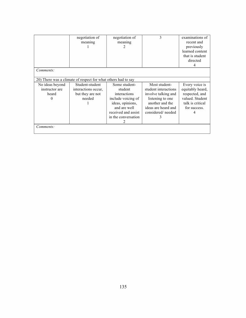
  135

negotiation of meaning

1

negotiation of meaning

2

3 examinations of recent and previously

learned content that is student

directed 4

Comments: 20) There was a climate of respect for what others had to say

No ideas beyond instructor are

heard 0

Student-student interactions occur,

but they are not needed

1

Some student-student

interactions include voicing of

ideas, opinions, and are well

received and assist in the conversation

2

Most student-student interactions involve talking and

listening to one another and the

ideas are heard and considered/ needed

3

Every voice is equitably heard, respected, and

valued. Student talk is critical for success.

4

Comments:

 

  136

Classroom Culture: Student/Teacher Relationships 21) Active participation of students was encouraged and valued Entirely instructor

directed, no student questions

0

Some student questions, may be opportunities to

“shout out” ideas 1

Some student questions/ input are encouraged,

and they appear to shift the direction

of the lesson 2

Many students engaged some of the

time in valuable conversations that

leads to class discussions that

appears to shift the direction

3

All students are actively

engaged in meaningful

conversation that guides the direction of the

lesson from beginning to the

end. 4

Comments: 22) Students were encouraged to generate conjectures, (or) alternative solutions, and/or different ways of interpreting evidence

Instructor may present

interpretations, conjectures, etc., but asks students

to do nothing 0

At least one time, students were

asked to consider an alternate

solution, make a conjecture, or

interpret evidence in more than one

way. 1

Teacher-student interactions lead

students through a very directed format that

considers alternate solutions, and/or

conjectures and/or evidence

2

Teacher-student interactions

facilitate students through a flexible

format that considers alternate solutions, and/or

conjectures, and/or evidence

3

Whole lesson is dedicated to

students discussing,

exploring and critiquing/

considering alternate

solutions, and/or different ways of

interpreting evidence, with

minimal teacher guidance

4 Comments: 23) In general the teacher was patient with the students (mostly about wait time) No opportunity to assess or teacher

was not patient (no wait time, answers

own questions). Unwanted behavior is

tolerated/ ignored 0

There is a bit of wait time after

asking a question, instructor avoids answering his/her own questions. Or

instructor works with student(s) to clarify their vague

question 1

Clear wait time (waiting for

multiple student thoughts, waiting

for all students have a chance to

consider the question; not just

taking the first raised hand or “shout out”).

2

Providing some time for student-

student interaction (still on task), but

may not be enough time for all to achieve goals.

3

Instructor provides

adequate time for meaningful

conversations to occur between

students (enough time to achieve

goal) 4

Comments 24) The teacher acted as a resource person, working to support and enhance student investigations (activity beyond answering a question) No investigations

(activity that Very teacher

directed, limited Primarily directed

by teacher with Students have freedom, but

Students are actively engaged

 

  137

engages students to apply content through problem

solving) 0

student investigation, very

rote 1

occasional opportunities for students to guide

the direction 2

within confines of teacher directed

boundaries 3

in their own learning process,

students determine what

and how, teacher is available to

help when needed 4

Comments: 25) The metaphor “teacher as listener” was very characteristic of this classroom

Teacher was the only “talker”

0

At least once, teacher listened,

and acknowledged or validated an idea presented.

1

Teacher is listening

throughout (from beginning to end), but doesn’t act on

any ideas (but does acknowledge)

2

Teacher listens from beginning to end of lesson, but

doesn’t necessarily act on ideas throughout

3

Teacher listens and acts on what

students are saying from the beginning to the end of the lesson

(from gaining prior knowledge

all the way to assessing student understanding).

4 Comments:

 

  138

APPENDIX E

HUMAN SUBJECTS APPROVAL FROM MARICOPA COUNTY COMMUNITY

COLLEGE DISTRICT AND ARIZONA STATE UNIVERSITY

 

  139

MCCCD - IR

B

DATE: January 13, 2012TO: Kraft, Katrien, Geosciences

Wilson, Merry, Geosciences, Matheney, RonaldFROM: MCCCD Institutional Review BoardPROTOCOL TITLE: Geoscience Affective Research NETwork (GARNET) 2FUNDING SOURCE: National Science FoundationPROTOCOL NUMBER: 2010-08-053FORM TYPE: AMENDMENTREVIEW TYPE: EXEMPT

Dear Principal Investigator,

The MCCCD IRB reviewed your protocol and determined the activities outlined do constitute human subjects research according to the Code of Federal Regulations, Title45, Part 46.

The determination given to your protocol is shown above under Review Type.

You may initiate your project.

If your protocol has been ruled as exempt, it is not necessary to return for an annual review. If you decide to make any changes to your project design which might resultin the loss of your exempt status, you must seek IRB approval prior to continuing by submitting a modification form.If your protocol has been determined to be expedited or full board review, you must submit a continuing review form prior to the expiration date shown above. If youmake any changes to your project design, please submit a modification form prior to continuing.

We appreciate your cooperation in complying with the federal guidelines that protect human research subjects. We wish you success in your project.

Cordially,MCCCD IRB

Maricopa County Community College District2411 West 14th Street

Tempe AZ, 85281TEL: (480) 731-8701FAX: (480) 731 8282

Page: 1

 

  140

To: Jenefer HusmanEDB

From: Mark Roosa, ChairSoc Beh IRB

Date: 05/01/2013

Committee Action: Exemption Granted

IRB Action Date: 05/01/2013

IRB Protocol #: 1304009127

Study Title: Geoscience Affective Research Network (GARNET)

The above-referenced protocol is considered exempt after review by the Institutional Review Board pursuant toFederal regulations, 45 CFR Part 46.101(b)(1) (2) .

This part of the federal regulations requires that the information be recorded by investigators in such a manner thatsubjects cannot be identified, directly or through identifiers linked to the subjects. It is necessary that the informationobtained not be such that if disclosed outside the research, it could reasonably place the subjects at risk of criminal orcivil liability, or be damaging to the subjects' financial standing, employability, or reputation.

You should retain a copy of this letter for your records.