Deterministic Modeling of the MOS Background

Steve SnowdenNASA/Goddard Space Flight Center

EPIC Operations and Calibration MeetingMallorca 1-3 February 2005

Kip Kuntz of NASA/Goddard Space Flight Center, University of Maryland – Baltimore County, and soon to be associated with Jophns Hopkins University performed most of the calibrations and wrote most of the software used for this presentation.

What do I Mean by Deterministic?

• Use as many known parameters as possible rather than relying on local background determinations and one-size fits all background data sets

• E.g., FWC Data, RASS, Soft Proton distribution, Archived Observation Data Sets

• Stir the pot and see what comes out

Step 1 – Filter the Data• Nearly any reasonable method will work• We use the 2.5-8.5 keV band for the filtering• Create a light curve and then a light-curve

histogram• Fit a Gaussian to the main peak• Exclude time periods where the count rate is

greater than 2.5 times the RMS above the mean of the Gaussian (do this iteratively)

Step 1 – Filter the Data

Light curves can range from very clean to incredibly ugly, some with very little useful time

2.5-8.5 keV Band from the FOV

2.5-8.5 keV Band from the corners

Step 1 – Filter the Data

But most of the time the light curve will be somewhere in between.

Step 2 – Model the Quiescent Particle Background

• Determine the corner spectral parameters: high-energy power law slope [2.4-12.0 keV] and hardness ratio

[(2.5-5.0)/(0.4-0.8)] from the observation data set• Search a archived-observation data base for observations with

similar parameters• Augment the observation data set corner spectra with data from

a second archived-observation data base• Scale the FWC spectra (treat each CCD separately) for the

region of interest by the ratio of the augmented observation corner spectra to the FWC corner spectra

• Use the corner spectra from the outside CCDs to model the background for the central CCD

Step 2 – Model the Quiescent Particle Background

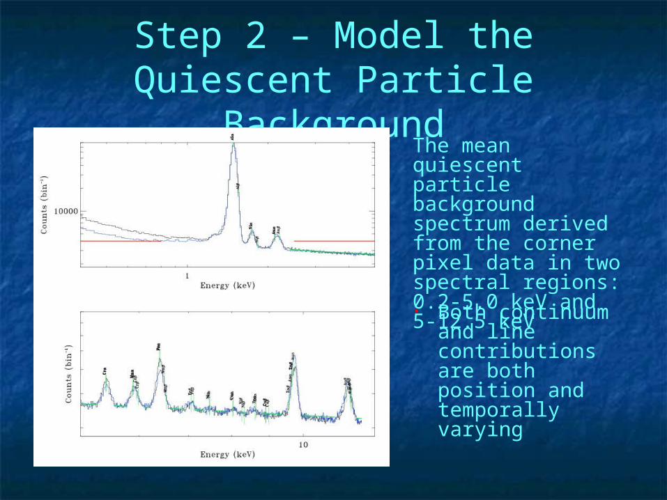
• Both continuum and line contributions are both position and temporally varying

The mean quiescent particle background spectrum derived from the corner pixel data in two spectral regions: 0.2-5.0 keV and 5-12.5 keV

Step 2 – Model the Quiescent Particle Background

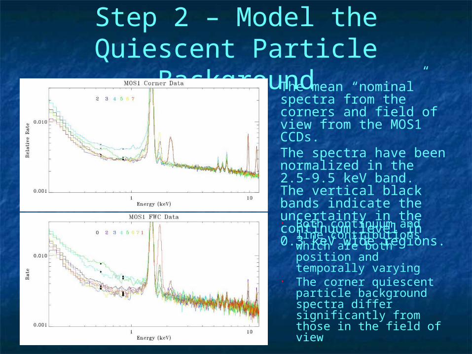
• Both continuum and line contributions which are both position and temporally varying

• The corner quiescent particle background spectra differ significantly from those in the field of view

The mean “nominal” spectra from the corners and field of view from the MOS1 CCDs.The spectra have been normalized in the 2.5-9.5 keV band. The vertical black bands indicate the uncertainty in the continuum level in 0.3 keV wide regions.

Step 2 – Model the Quiescent Particle Background

Temporal variation of the (top) 0.3-10.0 keV rate, (middle) the (2.5-5.0 keV)/0.4-0.8 keV) hardness ratio, and (bottom) 24.-12.0 keV power law index

Step 2 – Model the Quiescent Particle Background

• Occasionally CCD #5 goes weird, and must be treated separately (we don’t have a good method yet)

“Nominal” and “Elevated” spectra from the corners plotted for the MOS1 CCDs 2-7. The data have again been normalized in the 2.5-9.5 keV band

Step 2 – Model the Quiescent Particle Background

Comparison of the quiescent particle background in the FOV (black line) and corner regions (blue line). The green line is the corner spectrum normalized to the FOV spectrum in the 2.0-10.0 keV band.

Step 2 – Model the Quiescent Particle Background

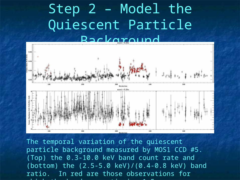
The temporal variation of the quiescent particle background measured by MOS1 CCD #5. (Top) the 0.3-10.0 keV band count rate and (bottom) the (2.5-5.0 keV)/(0.4-0.8 keV) band ratio. In red are those observations for which the hardness ratio is <1.5.

Step 3 – Get the RASS Spectrum for the Area

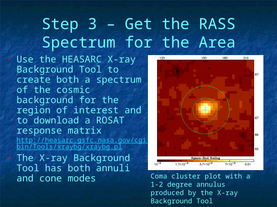
• Use the HEASARC X-ray Background Tool to create both a spectrum of the cosmic background for the region of interest and to download a ROSAT response matrix http://heasarc.gsfc.nasa.gov/cgi-bin/Tools/xraybg/xraybg.pl

• The X-ray Background Tool has both annuli and cone modes

Coma cluster plot with a 1-2 degree annulus produced by the X-ray Background Tool

Step 4 – Fit the Spectrum

• The model should include a model for the source of interest, the cosmic background, instrumental Al Kα and Si Kα, a scale factor for the solid angle, and an unfolded broken power law for any residual soft proton contamination.

• bknpow/b + gauss + gauss + con*(apec + (apec + apec + pow)*wabs) + source

Step 4 – Fit the Spectrumbknpow/b + gauss + gauss + con*(apec1 + (apec2 + apec3 +

pow)*wabs) + source• bknpow/b represents the residual soft proton contamination• gauss + gauss are the Al Kα and Si Kα instrumental lines• con scales for the different solid angles (in units of arc

minutes)• apec1 is the LHB, apec2 is the soft halo, apec3 is the hard

halo • pow is the extragalactic background• wabs is the Galactic column density• source is your favorite source spectrum

Step 4 – Fit the Spectrum

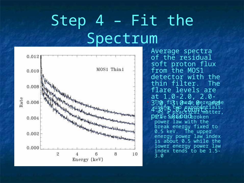
• The fits here were done using two exponentials. As a practical matter, I’ve used a broken power law with the break energy fixed to 0.5 keV. The upper energy power law index is about 0.5 while the lower energy power law index tends to be 1.5-3.0

Average spectra of the residual soft proton flux from the MOS1 detector with the thin filter. The flare levels are at 1.0-2.0, 2.0-3.0, 3.0-4.0, and 4.0-5.0 counts per second

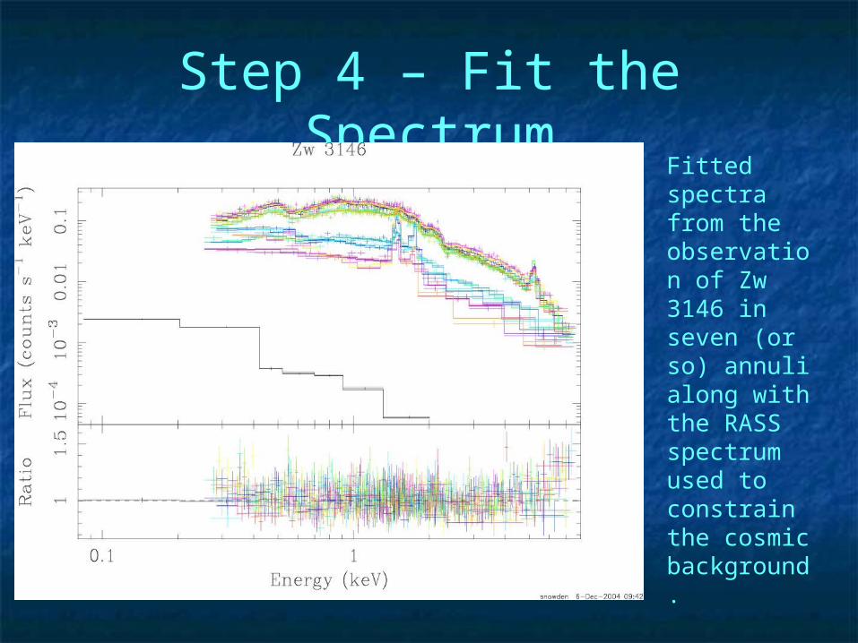
Step 4 – Fit the SpectrumFitted spectra from the observation of Zw 3146 in seven (or so) annuli along with the RASS spectrum used to constrain the cosmic background.

Step 4 – Fit the SpectrumFitted spectra from the observation of A1835 in seven (or so) annuli along with the RASS spectrum used to constrain the cosmic background.

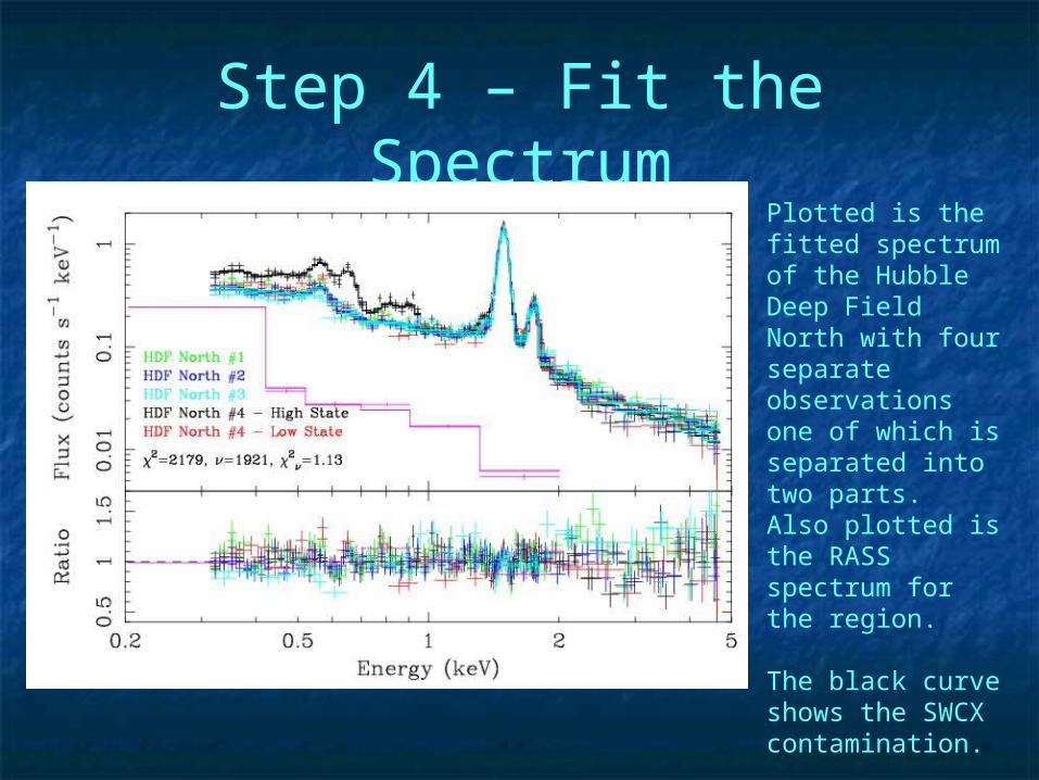
Step 4 – Fit the SpectrumPlotted is the fitted spectrum of the Hubble Deep Field North with four separate observations one of which is separated into two parts. Also plotted is the RASS spectrum for the region.

The black curve shows the SWCX contamination.

Step 4 – Fit the SpectrumPlotted is the unfolded fitted spectrum of the Hubble Deep Field North with and without the SWCX contamination.

The strong OVII and OVIII emission can clearly significantly affect observations of extended sources and the diffuse background.

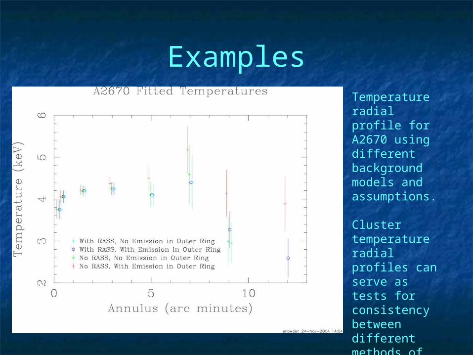
ExamplesTemperature radial profile for A2670 using different background models and assumptions.

Cluster temperature radial profiles can serve as tests for consistency between different methods of background modeling.

Still what is truth and beauty?

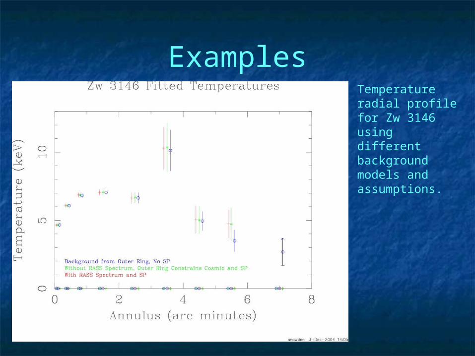
ExamplesTemperature radial profile for Zw 3146 using different background models and assumptions.

Background Subtracted Images

Background images are required, which adds a whole new level of complexity.

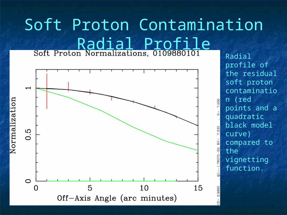
Soft Proton Contamination Radial Profile

Radial profile of the residual soft proton contamination (red points and a quadratic black model curve) compared to the vignetting function.

What NowWhat Now

• An Ftool is in testing which incorporates the An Ftool is in testing which incorporates the procedures discussed here for spectral analysisprocedures discussed here for spectral analysis

• Work is progressing on the image analysisWork is progressing on the image analysis• Need to understand MOS1 CCD#5 betterNeed to understand MOS1 CCD#5 better• Need to compare this method with othersNeed to compare this method with others