Developing a One-Dimensional, Two-

Phase Fluid Flow Model in Simulink

James Edward Yarrington

Thesis submitted to the faculty of the Virginia Polytechnic Institute and State

University in partial fulfillment of the requirements for the degree of

Master of Science

In

Mechanical Engineering

Alan A. Kornhauser, Chair

Yang Liu

Robert E. Masterson

12/9/2013

Blacksburg, Virginia

Keywords: Simulink, One-Dimensional, CFD, Two-Phase

Developing a One-Dimensional, Two-Phase Fluid Flow

Model in Simulink

James Edward Yarrington

ABSTRACT In this thesis, a one-dimensional, two-fluid model is developed in MATLAB-Simulink. The model features

a mass, momentum, and energy balance for each fluid—an ideal gas and an incompressible liquid. The

simulation may model a straight pipe section, or a pipe section that involves a cross-sectional area

change. Rough models of interphase heat transfer and interphase friction are included. Currently,

phase change is not modeled in the simulation

Also, a single-fluid model was developed before the two-fluid model, as an intermediate step in

developing the two-fluid model. The single-phase simulation applies a mass, momentum, and energy

balance for the single fluid, and ideal gas.

The single-fluid model was validated by incompressible flow, Fanno flow, and isentropic flow models.

The incompressible model demonstrated the simulations ability to properly balance pressure and

frictional forces. The Fanno flow model showed that the simulation could capture compressibility

effects. The isentropic flow model validation verified that the simulation could model area change

properly.

The two-fluid model was validated using the Homogeneous Equilibrium Model (HEM). An analytical

model of HEM flow with frictional pressure drop was developed to compare against the simulation

results. To achieve the HEM, interphase effects were tuned so that the liquid and gas phases had similar

temperatures and velocities. Under these conditions, the simulation matched the analytical model.

The thesis goal is to create a solid foundation for an open-source, one-dimensional, two-fluid model that

is easier to use and modify than current nuclear system analysis software.

iii

Table of Contents ABSTRACT ...................................................................................................................................................... ii

List of Figures .............................................................................................................................................. vii

List of Tables .............................................................................................................................................. viii

Introduction .................................................................................................................................................. 1

One-Dimensional, Two-Fluid Models ........................................................................................................ 1

Motivation................................................................................................................................................. 1

Addressing Concerns ................................................................................................................................. 1

Model Overview ............................................................................................................................................ 3

Literature Review .......................................................................................................................................... 6

Single-Phase Simulation ................................................................................................................................ 7

Junction Calculations ................................................................................................................................ 7

Property Averaging ............................................................................................................................... 7

Mass and Momentum Flow Rate .......................................................................................................... 8

Energy Flow Rate .................................................................................................................................. 8

Friction .................................................................................................................................................. 9

Volume Calculations ............................................................................................................................... 11

Mass and Energy ................................................................................................................................. 11

Momentum ......................................................................................................................................... 12

Integration .......................................................................................................................................... 13

Ideal Gas State .................................................................................................................................... 14

Boundary Conditions ............................................................................................................................... 16

Relation to Balance Equations ................................................................................................................ 19

Mass Continuity .................................................................................................................................. 19

Momentum Balance............................................................................................................................ 19

Energy Balance .................................................................................................................................... 20

Two-Phase Model ....................................................................................................................................... 22

Junction Calculations .............................................................................................................................. 22

Volume Calculations ............................................................................................................................... 24

Weight ................................................................................................................................................. 24

Pressure Balance ................................................................................................................................. 24

Interphase Drag Momentum Transfer ................................................................................................ 25

Interphase Drag Energy Dissipation .................................................................................................... 25

iv

Expansion Work .................................................................................................................................. 26

Interphase Heat Transfer .................................................................................................................... 27

Balance Equations ............................................................................................................................... 27

Equations of State ............................................................................................................................... 28

Relation to Balance Equations ................................................................................................................ 29

Mass Continuity .................................................................................................................................. 29

Momentum Balance............................................................................................................................ 30

Energy Balance .................................................................................................................................... 31

Simulation Validation .................................................................................................................................. 33

Incompressible Flow Model .................................................................................................................... 34

Test Procedure .................................................................................................................................... 34

Results ................................................................................................................................................. 35

Fanno Flow Model .................................................................................................................................. 37

Test Procedure .................................................................................................................................... 38

Results ................................................................................................................................................. 38

Isentropic Flow Model ............................................................................................................................ 40

Test Procedure .................................................................................................................................... 41

Results ................................................................................................................................................. 42

Two-Phase Validation ................................................................................................................................. 46

Homogeneous Equilibrium Model .......................................................................................................... 46

Developing the Validation Criterion ................................................................................................... 46

Test Procedure .................................................................................................................................... 48

Results ................................................................................................................................................. 48

Conclusions ................................................................................................................................................. 50

Comparison to Previous Work ................................................................................................................ 50

RELAP Comparison .................................................................................................................................. 51

Mass Continuity .................................................................................................................................. 51

Momentum Conservation ................................................................................................................... 51

Energy Conservation ........................................................................................................................... 52

Next Steps ............................................................................................................................................... 53

Accurate Interphase Models ............................................................................................................... 53

Validate Transients ............................................................................................................................. 53

Phase Change ...................................................................................................................................... 53

Wall Heat Transfer .............................................................................................................................. 54

Special Components ............................................................................................................................ 54

v

Bibliography ................................................................................................................................................ 55

Appendix A: Nomenclature ......................................................................................................................... 57

Variable Names ....................................................................................................................................... 57

Subscripts ................................................................................................................................................ 59

Superscripts and Symbols ....................................................................................................................... 60

Appendix B: Simulation Data ...................................................................................................................... 61

Incompressible Simulation ...................................................................................................................... 61

Fanno Flow Validation ............................................................................................................................ 62

Isentropic Flow Validation ...................................................................................................................... 63

HEM Simulation Validation ..................................................................................................................... 68

Appendix C: Single Phase Simulation Code ................................................................................................. 69

Junction Block Code ................................................................................................................................ 69

Junction_OLD ...................................................................................................................................... 69

Outlet_OLD ......................................................................................................................................... 70

Inlet_OLD ............................................................................................................................................ 71

Inner_OLD ........................................................................................................................................... 72

RapidExpansion ................................................................................................................................... 72

FlowPropsOLD ..................................................................................................................................... 73

extrapolate .......................................................................................................................................... 74

LengthAve ........................................................................................................................................... 75

FrictionCalc .......................................................................................................................................... 75

Volume Block Code ................................................................................................................................. 77

ICs ........................................................................................................................................................ 77

MomentumAdj .................................................................................................................................... 77

Volume ................................................................................................................................................ 78

Simulink Images ...................................................................................................................................... 80

JuncVolCombo_SP ............................................................................................................................... 80

JunctionPart_SP .................................................................................................................................. 81

VolumePart_SP ................................................................................................................................... 82

Subsystem (Integrator) ....................................................................................................................... 82

Appendix D: Two Phase Simulation Code ................................................................................................... 83

Junction Block Code ................................................................................................................................ 83

Junction_V ........................................................................................................................................... 83

Junction_L ........................................................................................................................................... 84

Outlet .................................................................................................................................................. 86

vi

Inlet ..................................................................................................................................................... 87

Inner .................................................................................................................................................... 88

FlowProps ............................................................................................................................................ 88

Volume Block Code ................................................................................................................................. 90

ics ........................................................................................................................................................ 90

flowadjustments ................................................................................................................................. 91

Volume ................................................................................................................................................ 93

tempvel ............................................................................................................................................... 94

Simulink Images ...................................................................................................................................... 95

JuncVolCombo .................................................................................................................................... 95

JunctionPart ........................................................................................................................................ 96

VolumePart ......................................................................................................................................... 97

vii

List of Figures Figure 1. The transfer of information between simulation components. ................................................... 3

Figure 2. Representation of a possible simulation setup. ........................................................................... 4

Figure 3. Diagram explaining junction subscript nomenclature. ................................................................. 7

Figure 4. Diagram explaining volume subscript nomenclature. ................................................................ 11

Figure 5. Illustration of the pressure forces acting on a volume block. ..................................................... 12

Figure 6. Boundary condition usage. ......................................................................................................... 16

Figure 7. Visualization of first-order space extrapolation. ........................................................................ 17

Figure 8. Visualization of two-step extrapolation. ..................................................................................... 18

Figure 9. Plot of incompressible validation results. ................................................................................... 36

Figure 10. Plot of incompressible validation for low Mach numbers. ....................................................... 36

Figure 11. Plot of Fanno flow validation, showing temperature property ratios against Mach number.. 39

Figure 12. Plot of Fanno flow validation, showing pressure property ratios against Mach number. ....... 39

Figure 13. Plot of Fanno flow validation, showing velocity property ratios against Mach number. ......... 40

Figure 14. Plot of contraction isentropic validation, showing cross-sectional area ratios against Mach

number. ....................................................................................................................................................... 42

Figure 15. Plot of contraction isentropic validation, showing cross-sectional area ratios on a smaller

Mach number range. .................................................................................................................................. 43

Figure 16. Plot of contraction isentropic validation, showing pressure ratios against Mach number. ..... 43

Figure 17. Plot of contraction isentropic validation, showing temperature ratios against Mach number.

.................................................................................................................................................................... 44

Figure 18. Plot of expansion-contraction isentropic validation, showing cross-sectional area ratios

against Mach number. ................................................................................................................................ 44

Figure 19. Plot of expansion-contraction isentropic validation, showing pressure ratios against Mach

number. ....................................................................................................................................................... 45

Figure 20. Plot of expansion-contraction isentropic validation, showing temperature ratios against Mach

number. ....................................................................................................................................................... 45

Figure 21. Increasing liquid mass flow rate error with increasing velocity difference. ............................. 49

viii

List of Tables Table 1. Incompressible Validation Data. .................................................................................................. 61

Table 2. Fanno Flow Validation Data. ........................................................................................................ 62

Table 3. Isentropic Flow Validation Data, Contraction. ............................................................................. 63

Table 4. Isentropic Flow Validation Data, Expansion-Contraction Part 1 / 4. ........................................... 64

Table 5. Isentropic Flow Validation Data, Expansion-Contraction, Part 2 / 4. .......................................... 65

Table 6. Isentropic Flow Validation Data, Expansion-Contraction, Part 3 / 4. .......................................... 66

Table 7. Isentropic Flow Validation Data, Expansion-Contraction, Part 4 / 4. .......................................... 67

Table 8. HEM Validation Data. ................................................................................................................... 68

1

Introduction

One-Dimensional, Two-Fluid Models One-dimensional, two-fluid modelling packages, such as RELAP (Idaho National Laboratory, 2005), TRAC

(Liles, 1988), and TRACE (United States Nuclear Regulatory Commission, 2012), model fluid flow for the

purposes of nuclear reactor analysis. The simulations discretize the simulated flow path into control

volumes, which balance the mass, momentum, and energy flowing across their boundaries. Time is also

discretized, where each time step brings a new state for each control volume in the system. For each

time step, each control volume uses information from adjacent control volumes to determine how much

mass, momentum, and energy transfers across each boundary. One-dimensional models simplify fluid

flow by limiting the mass, momentum, and energy balance equations to one axis. While a three-

dimensional model would capture the intricacies of three-dimensional movement, like travelling

through a pipe bend, or contracting through a nozzle, one-dimensional models represent these effects

by incorporating empirical correlations into their balance equations.

Two-fluid models employ a mass, momentum, and energy balance for both fluids, effectively dividing

each control volume in two—one for each fluid. Two-fluid simulations transfer information, mass,

momentum, and energy, not only between adjacent control volumes, but between the fluids within the

same control volume. The resulting simulation: two fluids flow through the same medium, affected by

the constraints placed on the system as well as the interactions between the fluids. Homogenous

equilibrium models (HEM) represent two fluids flowing through the same medium, but are not true two-

fluid models; HEMs only model one fluid with the properties of the two-fluid mixture.

Motivation Though several one-dimensional, two-fluid models exist, these models involve some deficiencies. For

one, the source code behind the simulations is often unavailable due to proprietary restrictions. This

presents the user from knowing the exact mechanisms of the program. For instance, if a piece of

simulation software allows the user to adjust a friction factor, without the source code, the user may

poorly define the parameter and incorrectly model their system.

Furthermore, while some factors can be modified by users, several correlations are locked into the

original state. This reduces flexibility, preventing the user from creating more customized models.

Finally, many current one-dimensional models lack an intuitive front-end that allows the user to interact

with their system. Rather than change values within a text file to adjust the model, a user should be

able to interact with a graphical user interface to easily find (and change) any desired parameters. An

improved user interface would lessen the burden on the user manual to provide usage instructions.

Addressing Concerns The new simulation developed in this thesis will address these three concerns. The user’s simulation will

be done through MATLAB-Simulink. Simulink allows the user to graphically arrange and connect pieces

of code to build a model. Once the model is created, Simulink provides several ordinary differential

equation solvers to simulate the system, time-step by time-step. This provides a perfect environment in

which to simulate a one-dimensional fluid model.

The Simulink interface remedies the three concerns I presented in the Motivation section. With the

fluid model components developed, the user can easily arrange the components to create a series of

2

connected control volumes. System constraints can be changed directly on the front-end; the

simulation does not require a large text file with lists of settings for each component. If the user wishes

to examine and modify the source code of a certain part of the simulation, simply double-clicking the

component reveals the desired information.

3

Model Overview This section contains a brief overview of how the simulation functions. For a complete explanation,

including the governing equations, please see “Single-Phase Simulation” on page 7 and “Two-Phase

Model” on page 22.

The new software employs alternating “junction” and “volume” blocks to simulate the flow of fluid

along a pipe—dividing the work of the control volumes explained in the “One-Dimensional, Two-Fluid

Models” section. Each volume block calculates the state of the fluids contained in its boundaries,

solving the time derivative of the flow across its boundaries. Each junction performs the space-

derivatives of the simulation, taking the state of adjacent volume blocks to determine the flow rates

between them. Figure 1 shows the transfer of information between the volumes and junctions.

Junction blocks require the state of the fluids in the adjacent blocks at the previous time step to

determine flow rates. Volume blocks use those flow rates—along with the initial conditions—to

determine the total mass, momentum, and energy contained within the volume. The volume blocks

then determine density, velocity, and temperature from the mass, momentum and energy totals,

passing this information to the neighboring junction blocks for the next time step’s calculations. The

cycle of volume and junction blocks exchanging information perpetuates until the simulation reaches

the preset stopping time

Figure 1. The transfer of information between simulation components. The horizontal arrows represent volume data, including

geometry, fluid state, and velocity, which pass to adjacent junction blocks at each iteration. The triangles contain junction data,

including friction and various flow rates, which pass to adjacent volume blocks. The vertical arrow represents the initial

conditions of a volume block. The vertical arrow contains the same type of information as the horizontal arrows, except that

the information is only used once at the beginning of the simulation.

At the start of the simulation, each volume block receives information describing the geometry of that

section of the pipe: the cross-sectional area; the length; and the angle above horizontal. Adjusting the

geometric settings of each volume block allows the user to model expansion, contraction, upward flow,

downward flow, or a combination of any of those four. Figure 2 shows several volumes connected that

use different areas, lengths, and angles. Along with the geometry, the volume blocks receive the initial

condition of the fluids within their boundaries. This information allows the volume blocks to calculate

the starting point for the total mass, momentum, and energy they each contain.

4

Figure 2. Representation of a possible simulation setup. The nine shapes represent the discretization of a pipe section that

contracts, expands, falls, and climbs. To accomplish this, the pipe is divided into sections that have varying angle, cross-

sectional area, and length. Sections 2 and 3 have negative angles relative to the horizontal, while sections 7, 8, and 9 have

positive angles. Contraction occurs between sections 4 through 6, as each successive section has a smaller cross-sectional area.

Sections 7 through 9 expand, increasing the cross-sectional area. Finally, sections 1 and 9 have shorter lengths than the other

sections.

Initially, a single-phase model was developed, using only an ideal gas as the simulation fluid. This simple

model was used as an intermediate point during development of the two-phase model. In the single-

phase model, the junction blocks calculate the mass, momentum, and energy flow rates of the ideal gas

(space derivatives), while the volume blocks determine the state of the ideal gas, using the mass,

momentum, and energy stored within the volume, along with the ideal gas law (time derivatives). To

appropriately constrain the system, the simulation requires an inlet temperature and density, as well as

an outlet pressure. This is equivalent to a pressure drop across the pipe plus the state of the source

fluid. To facilitate change of direction, the temperature and density are defined on both boundaries;

however, only the pressure (calculated from temperature and density using the equation of state) is

used on the exit boundary.

The two-phase model adds an incompressible liquid phase to the ideal gas-phase. Developed after the

single-phase model, the two-phase model employs the same structure as the original, with a few

exceptions. The junction blocks transmit two sets of flow data; one mass, momentum, and energy flow

rate for each phase. Likewise, the volume blocks perform an extra set of balances to manage the

additional fluid.

At each time step, the volume each fluid occupies fluctuates, so the ideal gas relationship cannot initially

be used. Because the liquid phase has a constant density, the volume it occupies can be found from the

total liquid mass within the volume block. The remaining volume belongs to the gas phase, and is used

for the ideal gas equation of state calculations. Liquid pressure equals the gas pressure derived from the

ideal gas relationship.

Furthermore, the two fluids interact with one another within the volume block. Momentum transfers

from one phase to the other due to friction driven by a velocity difference. Energy transfers due to heat

transfer driven by a temperature difference.

5

With the second set of balance equations added for the liquid, three additional constraints must be

added to the system—in addition to the inlet gas density, inlet gas temperature, and outlet pressure.

First, as the liquid is incompressible, the fluid density is predefined at the start of the simulation. Then

the addition of inlet void fraction and inlet liquid temperature completely define the state of the two

fluids entering the system.

6

Literature Review This literature review briefly covers the history of one-dimensional, two-fluid modelling. It also

highlights the origins of several concepts employed by this thesis. This section also introduces

previously developed models; however, the section “Comparison to Previous Work” contains more

details on how these models compare to the model described by this thesis.

One of the earliest two-fluid modelling schemes was developed by (Martinelli & Nelson, 1948). This oft-

cited work represents two-fluid flow by applying an empirically derived correction factor to a single-fluid

model. As explained by (Todreas & Kazimi, 2012), the application of two-fluid models to nuclear

systems began later in the 1960s. This led to the accepted convention of models applying balances

across control volumes, as in (Collier & Thome, 1994). Further evolution led to the more recent method

of local instant formulation, by (Ishii & Takashi, 2011), which solves for properties at centers of volumes

with unknown boundaries.

Within the past 25 years, several one-dimensional models have been developed. This thesis compares

these models with the new simulation developed in this thesis in the Comparison to Previous Work

section. (Scheuerer & Scheuerer, 1992) developed a one-dimensional, two fluid model utilizing mass

and momentum balance equations. (Herrán-González, De La Cruz, De Andrés-Toro, & Risco-Martín,

2009) developed one dimensional models for Simulink to simulate natural gas distribution pipelines,

accounting for elevation change, but also neglected the energy equation. (Davis & Campbell, 2007)

created a one-dimensional fluid flow model utilizing mass, momentum and energy balance equations,

utilizing the REFPROP database to determine fluid states. Davis’s simulation models two fluids by

assuming homogenous equilibrium, treating the two fluids as a single substance. Other, more unique

methods of simulating fluid flow include (Alamian, Behbahani-Nejad, & Ghanbarzadeh, 2012), who

solved the governing equations as state-space equations.

The standard of comparison for the simulation created in this thesis, RELAP (Idaho National Laboratory,

2005), models one- and two-dimensional flow using volumes and the junctions that connect them. The

section “RELAP Comparison” contains more information on the underlying equations balance equation

that govern RELAP. Other commercial software, such as TRAC (Liles, 1988), also model the thermal-

hydraulics of nuclear systems. Later, TRACE combined the functionality of RELAP and TRAC (United

States Nuclear Regulatory Commission, 2012).

Several resources proved to be vital in the development of the simulation. As the simulation was

created in the MATLAB-Simulink environment, the associated documentation, (The MathWorks, Inc,

2012), helped immensely. The integral form of the balance equations found in (Potter & Foss, 1982)

provided a check to ensure that the simulation followed the governing equations properly. The

extrapolation methods explained in (Hirsch, 1990) were employed at the boundaries of the system. A

modification of the smooth-pipe correlation presented in (Incropera, DeWitt, Bergman, & Lavine, 2007)

was used to programmatically determine friction factor from Reynolds number. To validate the

simulation, the Fanno and Isentropic gas tables from (Keenan & Kaye, 1948), provided a starting point,

though not used in the final validation calculations; the validation equations were provided by (Munson,

Young, & Okiishi, 1998).

7

Single-Phase Simulation The one-dimensional, single-phase simulation models the flow of an ideal gas within a pipe section.

The independent variables of the simulation include the total mass, momentum, and energy contained

within control volumes. The volume blocks, which perform calculations on their respective control

volumes, use the ideal gas law to determine the state (velocity, temperature, density) of the fluid from

the independent variables. Connecting the volume blocks, junction blocks receive the state information

to determine the mass, momentum, and energy flow rates between volume blocks. In the next time

step, the volume blocks use the flow rates to determine the new quantities of mass, momentum, and

energy stored in their control volumes. This section details the calculations of the junction and volume

blocks.

Junction Calculations As seen in Figure 1, the function of junction blocks is to provide mass, momentum, and energy flow

rates to adjacent volume blocks. This information describes how much of a quantity (mass, momentum,

or energy) passes from one volume to another. The junction blocks accomplish this by averaging the

properties of adjacent volumes, then calculating mass, momentum, and energy flow rates according to

the averaged properties.

Property Averaging

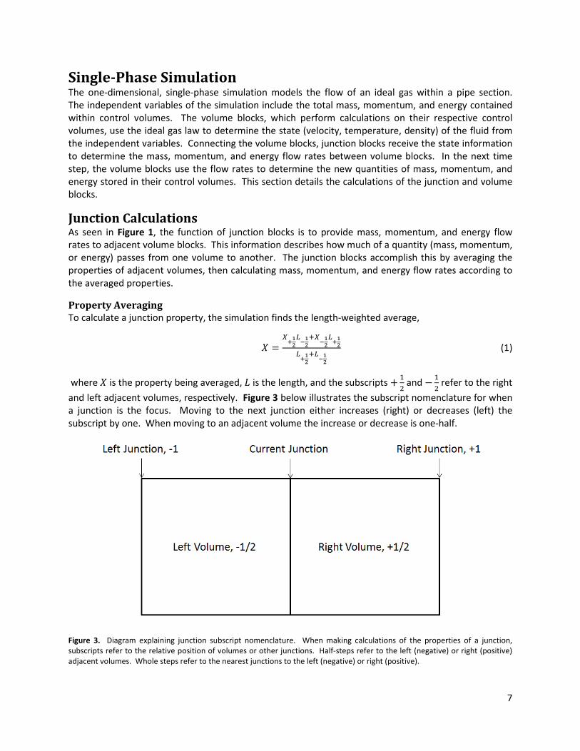
To calculate a junction property, the simulation finds the length-weighted average,

� = ������������������������ (1)

where � is the property being averaged, is the length, and the subscripts + � and − � refer to the right

and left adjacent volumes, respectively. Figure 3 below illustrates the subscript nomenclature for when

a junction is the focus. Moving to the next junction either increases (right) or decreases (left) the

subscript by one. When moving to an adjacent volume the increase or decrease is one-half.

Figure 3. Diagram explaining junction subscript nomenclature. When making calculations of the properties of a junction,

subscripts refer to the relative position of volumes or other junctions. Half-steps refer to the left (negative) or right (positive)

adjacent volumes. Whole steps refer to the nearest junctions to the left (negative) or right (positive).

8

The simulation uses Equation (1) to find the temperature, density and velocity of the junction. With

these values known, the simulation calculates pressure,

� = ��� (2)

where � is density, � is temperature and � is the specific gas constant for the fluid.

Mass and Momentum Flow Rate

The junction block then calculates the mass, momentum and energy flows between its adjacent

volumes. These three flow rates come from the flow properties within the junction—the length-

weighted properties of the adjacent volumes. Mass flow,

�� = ��� (3)

representing the mass that crosses the junction block to leave one control volume and enter another.

Similarly, momentum flow,

�� = �� � (4)

represents the momentum that the mass from Equation (3) carries from one control volume to another.

Energy Flow Rate

The mass flowing from one control volume to the next also carries energy, including enthalpy, kinetic

energy, and potential energy. The total energy contained in a unit mass passing between the two

volumes,

� = ℎ + �� + �� (5)

where kinetic energy,

�� = �� (6)

and potential energy,

�� = ��� (7)

where � is the junction height, and enthalpy,

ℎ = � + ! (8)

where internal thermal energy,

� = "�� (9)

where #� is the constant-volume specific heat of the fluid and assumed constant, and the reference

point for temperature is arbitrarily set at absolute zero. Thus, the total energy passing from one volume

to another per unit mass,

� = �� + "�� + ! + ��� (10)

9

The total energy flow,

$� = �� � = �� (�� + "�� + ! + ���) (11)

which is the total energy that the mass flow, from Equation (3), carries with it from one control volume

to another. The energy flow equations simplifies further to

$� = �� (�'"� + �( + �� + ���) (12)

when the fluid is an ideal gas. The flows determined by equations (3), (4), and (12) are used by the

adjacent volumes to determine how much mass, momentum and energy enters and leaves during the

following time step.

Friction

The junction calculates frictional force as well. Three scenarios exist for friction calculations—no

friction, constant friction factor, and smooth pipe friction. With a constant friction factor, including zero

for the no friction case, calculations for frictional force begin at Equation (17).

For the smooth pipe friction calculation, friction factor is determined by Reynolds number,

��) = !�)*+ (13)

where � is the velocity of the fluid within the pipe, ,- is the hydraulic diameter, and . is the dynamic

viscosity. The simulation estimates dynamic viscosity as,

. = ./0112 (14)

where the subscript 0 refers to a reference point. In the simulation, this point,

(�/, ./) = (300'7(, 1.983 • 10=>'�? − @() (15)

With Reynolds number known, the simulation calculates friction factor,

A =BCDCE

64��, ,��, < 1189.4

0.316��)=�I, 1189.4 < ��, ≤ 49,818.90.184��)=�K,��, ≥ 49,818.9

(16)

where the three equations come from (Incropera, DeWitt, Bergman, & Lavine, 2007). Typically, the

transition points for the three equations occur at 2,300 and 20,000, but these points did not create a

function that was continuous over the desired range of Reynolds numbers. The cut-off points in

Equation (16) allow for a smoother transition between friction factor formulas.

Whether the friction factor was calculated or a constant, the simulation calculates the wall shear stress,

10

MN = ��!OP (17)

and then frictional force,

QO = (��������)R)*STU (18)

The sign of QO depends on the sign of �, such that the frictional force is always applied opposite fluid

motion. Specifically, the code applies the opposite sign of � to QO. The simulation divides the friction

factor by four because of averaging explained in the volume block section.

The junction block sends the mass flow rate, Equation (3), momentum flow rate, Equation (4), energy

flow rate, Equation (12), and friction force, Equation (18), to the adjacent volume blocks so that the total

mass, momentum, and energy in that volume block may be calculated for the next time step. Please

note that wall heat transfer is not yet included in the model. When included, it will operate in a similar

manner to friction; the temperature difference between the fluid and the wall will drive heat transfer,

much like the velocity difference between the fluid and the wall drives friction.

11

Volume Calculations At the start of each time step, the volume blocks receive flow rates from the adjacent junction blocks.

The flow data includes mass flow, momentum flow, and energy flow, as well as frictional force. The

volume block uses the flow rates and forces to determine the new mass, momentum and energy of the

fluid within the block for the current time step. Combined with the geometry of the block, the mass,

momentum, and energy held within the control volume determine the state of the fluid: the

temperature, density, pressure, and velocity. The state of the fluid, is passed to the neighboring

junction blocks in order to calculate the flow rates (and friction) for the next step.

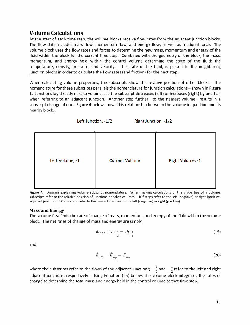
When calculating volume properties, the subscripts show the relative position of other blocks. The

nomenclature for these subscripts parallels the nomenclature for junction calculations—shown in Figure

3. Junctions lay directly next to volumes, so the subscript decreases (left) or increases (right) by one-half

when referring to an adjacent junction. Another step further—to the nearest volume—results in a

subscript change of one. Figure 4 below shows this relationship between the volume in question and its

nearby blocks.

Figure 4. Diagram explaining volume subscript nomenclature. When making calculations of the properties of a volume,

subscripts refer to the relative position of junctions or other volumes. Half-steps refer to the left (negative) or right (positive)

adjacent junctions. Whole steps refer to the nearest volumes to the left (negative) or right (positive).

Mass and Energy

The volume first finds the rate of change of mass, momentum, and energy of the fluid within the volume

block. The net rates of change of mass and energy are simply

�� VWX = �� =�� −�� �� (19)

and

$�VWX = $�=�� −$��� (20)

where the subscripts refer to the flows of the adjacent junctions; + � and − � refer to the left and right

adjacent junctions, respectively. Using Equation (25) below, the volume block integrates the rates of

change to determine the total mass and energy held in the control volume at that time step.

12

Momentum

Because the change in momentum not only includes the fluid flow, but frictional and pressure forces as

well, the net rate of change equation for momentum contains more terms than the corresponding mass

and energy equations. The frictional force is already calculated by the adjacent junctions and passed to

the volume block.

Pressure

Driving the flow of fluid through the pipe is the pressure differential from one end to the other.

Likewise, each volume block has a pressure differential—the pressure calculated in its adjacent junction

blocks. With a pressure differential, the net force applied on the block due to pressure,

Q = (�=�� − ���)� (21)

However, the simulation allows for varying area so the right and left boundaries of the volume block

may not have the same area. Figure 5 shows the force balance (for pressure forces) acting on a volume

block whose neighbors do not have equal cross-sectional areas; the double lines create the borders of

the volume blocks. The upstream pressure is applied over the upstream volume’s area, while the

downstream pressure is applied over the downstream volume’s area, depicted by arrows in the figure.

If the upstream and downstream cross-sectional areas differ, the (hypothetical) walls of the volume

block will slant, as seen in the light dotted lines in Figure 5. The slanted walls apply a pressure force

normal to their surface; considering the component of pressure force in the flow dimension, the

resulting force is shown by triangles in Figure 5. The pressure force applied is the product of the

volume’s pressure and the difference between the upstream and downstream area.

Figure 5. Illustration of the pressure forces acting on a volume block. The pressure differential between the left and right

junctions provides the driving force behind fluid motion. The circumferential pipe wall does not contribute to fluid motion, as

the uniform pressure along the circumference of the pipe cancels itself. The remaining surface area of the volume, the

difference between the upstream and downstream area, applies force to the fluid equal and opposite to the pressure force the

fluid applies on that same area, shown with arrows.

13

Therefore, the net force due to pressure acting on the volume,

Q = �=���=� − ����� + � Y�=�� + ���Z (�� − �=�) (22)

The final term in Equation (22) is the average pressure within the volume applied over the area

difference. If the flow is expanding from left to right, the area difference will be positive, which

correctly results in an additional pressure force acting in the positive (right) direction.

Weight

Weight is the final force acting on the fluid. If the pipe is completely horizontal, then the momentum

balance contains no weight term, as no component of the weight lies in the axis of flow. If, however,

the pipe has any other angle, then weight,

[ = ��� • @\](^) (23)

where ^ is the angle above horizontal and � is the volume of the cell.

Integration

With terms for pressure force, friction, and weight developed, the net change in momentum over time

of the volume,

��VWX = _�� + QO`=�� +_−�� + QO`�� + Q +−[ (24)

with the − � components from the left junction, and the + � components from the right junction. Next,

the volume block finds how much mass, momentum and energy is within its boundaries. The current

amount of a property,

�(a/ + Δa) = c _��`daX2eXX2 + �(a/) (25)

where a/ is the time of the last simulation step, Δa is the time between the current and last simulation

step, and �(a/) is the value of the property at time a/. Equation (25) applies to mass, momentum and

energy within the volume block.

Initial Conditions

Initial conditions are needed for the first time step; else equation (25) would be undefined. Because the

user cannot directly measure initial quantities of mass, momentum, and energy, the user defines the

state using temperature, density and velocity. The simulation then converts these values to mass,

momentum, and energy so that equation (25) can be used. The initial mass,

�/ = ��/ (26)

where the volume of the cell,

� = � (27)

the initial momentum,

�/ = �/�/ (28)

14

and the initial energy,

$/ = �/ f"��/ + �2� + ��g (29)

where the subscript 0 refers to the initial condition at the first time step.

MATLAB-Simulink Integration

Simulink provides several ordinary differential equation (ODE) solvers; when used with the one-

dimensional, one- and two-phase models, Simulink treats the entire system as a system of ODEs.

According to the documentation (The MathWorks, Inc, 2012), Simulink computes the states—variable

values—at each time step using the user-selected solver. Time steps vary based on the rate of changes

of the states; rapidly changing states require smaller time steps to improve accuracy.

The ODE solvers split into two categories, stiff and non-stiff. A stiff ODE involves variation on a short

time scale relative to the overall simulation time. The one-dimensional, one- and two-phase models are

stiff ODEs, as small fluctuations in a variable such as mass lead to fluctuations in other variables,

perpetuating the problem. Stiff ODE models require stiff ODE solvers, like the “ode23tb” solver used for

the validation cases starting on page 33, to overcome the instability associated with stiff ODEs.

The stiff ODE solver, ode23tb, is the solver used primarily during the development of this thesis. The

documentation describes this solver as “An implementation of TR-BDF2, an implicit Runge-Kutta formula

with a first stage that is a trapezoidal rule step and a second stage that is a backward differentiation

formula of order 2.” (The MathWorks, Inc, 2012).” Ode23tb was selected through trial-and-error,

selecting the most efficient solver that reliably finished simulations to steady state without encountering

an error.

Ideal Gas State

Once the volume block has a defined mass, momentum, and energy within its boundaries, it calculates

the fluid properties for use by the adjacent junction blocks. Because the fluid is an ideal gas, the

definition of density,

� = h� (30)

is used to find the density, as it is assumed the fluid consumes all available space within the cell. Also,

the definition of momentum,

� = �� (31)

is solved for velocity,

� = ih (32)

Velocity and density, along with the energy equation—equation (10) above—are used to find

temperature,

� = �jk flh − �� −��g (33)

15

where the flow work term, !, has been removed, as the fluid is not performing net work within the

block; flow work is only considered during mass transfer. Although the fluid has been completely

defined, pressure is also calculated, using equation (2) above, so that the volume’s pressure is available

when finding the pressure force balance, using equation (22) above.

With the time derivative complete, and the state of the fluid found, the simulation sends the state of the

fluid to the adjacent junction blocks to calculate the flow rates (space derivatives) and friction for the

volume block’s next time step.

16

Boundary Conditions Solving a fluid flow problem requires boundary conditions. With three governing equations—mass

continuity, momentum conservation, and energy conservation—the simulation needs three boundary

conditions. More boundary conditions leads to an over-constrained model, while fewer boundary

conditions leave the model undefined. The one-fluid simulation requires an inlet density, inlet

temperature, and outlet pressure. This provides an overall pressure drop that drives fluid flow, as well

as the state of the fluid entering the model. For the sake of symmetry—allowing reverse flow—the user

provides a density and temperature for both ends of the simulation. For the boundary with exiting flow,

the code only uses the defined density and pressure to calculate the boundary pressure. Figure 6

illustrates the dynamic boundary conditions used by the simulation for forward and reverse flow.

Figure 6. Boundary condition usage. For both forward and reverse flow conditions, density and temperature is defined for

both boundaries. This definition of state leads to a pressure defined on both ends of the simulation. For forward flow, the left

boundary supplies the state of the fluid entering the simulation—same for reverse flow and the right boundary. The

temperature and density of the other boundary remain unused after pressure is defined. For both cases, this yields a complete

state—temperature and density—inlet condition and a pressure exit condition; the simulation’s three boundary conditions

match the three governing mass, momentum, and energy equations.

The junction and volume blocks described in the previous sections do not account for boundary

conditions. Each volume block functions as if it is adjacent to two junction blocks. Each junction block

finds the length-weighted average of the adjacent volume blocks, using Equation (1), before calculating

mass, momentum, and energy flow rates. A junction at the boundary of the simulation—with only one

adjacent volume block—cannot calculate junction fluid properties in the same manner. If junctions

represent the boundaries to the model, then a different method must be employed to find the fluid

properties.

To find fluid properties for the junction blocks at the boundaries, extrapolation can be used. (Hirsch,

1990) provides several methods for extrapolation across time and space. A first-order space

extrapolation involves three co-linear, equidistant points—A, B, C, shown in Figure 7. If a property is

17

known at A and B, first-order space extrapolation estimates that property at C. The change in property

between B and C is assumed to match the change in property between A and B.

Figure 7. Visualization of first-order space extrapolation. The increasing (or decreasing) trend of some property from A to B

continues on to predict C, such that C – B = B – A.

In the illustration of Figure 7, C would be the boundary junction—that needs extrapolation to determine

some of its properties, B is the adjacent volume block and A is the nearest junction block. With the

subscript system explained in Figure 3, the value of a property at the boundary,

�m = 2��� − �� (34)

where the subscripts are either positive or negative depending on if the boundary is a left or right

boundary.

One caveat exists, preventing the simulation from solely using Equation (34) to estimate properties at

the boundary. A unit time delay occurs in the output of every junction block, so that volume blocks use

flow rate information from the previous time step. Without this delay, the simulation cannot work.

Therefore, when estimating the properties at the boundary junction, the current property of the nearest

junction, ��, is unknown, and Equation (34)—in its current form—cannot be used.

A first-order time extrapolation allows estimation of ��, using information from previous time steps.

Similar to the first-order space extrapolation, the time extrapolation (Hirsch, 1990) takes the previous

two values of �� to estimate its current value, assuming that the property continues on the same

trend. Therefore, the estimated current property of the nearest junction,

�� = 2��,X=� � ��,X= (35)

where the subscript a − ] indicates that the property occurred ] times steps in the past. Combining

Equation (34) and Equation (35) yields the final estimation for a boundary property,

�m = 2��� − 2��,X=� � ��,X= (36)

18

Figure 8 shows the two extrapolations combined to estimate the unknown value. The outlet, the right

boundary for forward flow, utilizes Equation (36) to estimate the junction density, temperature, and

velocity. With the inlet fluid state already defined, the inlet junction block only estimates velocity using

Equation (36). The use of extrapolation prevents over constraining the model by allowing the undefined

properties to be defined by the system, rather than a fixed constant.

Figure 8. Visualization of two-step extrapolation. In this diagram, crosses represent properties with a known value, while

circles represent properties with a value that must be estimated via extrapolation. The first extrapolation uses the previous

two values at point A to estimate the current value at point A. The second extrapolation uses the estimated value at point A—

along with the known value at point B—to estimate the value at point C.

Especially in transient situations, this extrapolation method can lead to instability; an extreme

extrapolation result will affect the system, possible causing an even more extreme extrapolation result

in the next time step. To place a limit on how far the extrapolated value can deviate from calculated

values the adjacent volume, the simulation checks the extrapolation result against a “stability fraction,” o. This forces the extrapolation result to fall within,

'��,/o, ��,2p ( (37)

where 0 H o J 1. For the results shown in this thesis, o � 0.8.

19

Relation to Balance Equations To ensure that the classical mass, momentum, and energy balance equations are obeyed, this section

compares the simulation calculations to the integral forms of the mass, momentum, and energy

equations found in (Potter & Foss, 1982).

Mass Continuity

The integral from of the conservation of mass from (Potter & Foss, 1982),

qqX c �d�r� + c �� • ]sd�rt = 0 (38)

where the integral subscripts #� and #u refer to integrals over a control volume and a control surface,

respectively, and ]s is the vector normal to the cross-sectional area. The first term in Equation (38)

refers to the mass rate of change of the control volume, while the second term refers to the flow of

mass across the boundary of the control volume. The first term can be simplified to

qqX c �d�r� = �� r� (39)

Restricting the flow to one-dimension—perpendicular to the cross-sectional area—and treating flow

from left to right as positive,

c ��vw • ]sd�rt = −(���)xWOX + (���)yz{-X (40)

where |�Aa and }\�ℎa refer to the side of the volume those values are taken from. The reduced

continuity equation,

�� r� = (���)xWOX − (���)yz{-X (41)

matches the combination of Equations (3) and (19) used in the simulation,

�� VWX = (���)=�� − (���)�� (42)

verifying that the simulation satisfies mass continuity.

Momentum Balance

Furthermore, (Potter & Foss, 1982) gives the one-dimension integral form of the momentum equation

as

ΣQ = qqX c ��d�r� + c ��_�vw • ]s`d�rt (43)

where ΣQ is the total force acting on the fluid within the control volume. The first term on the left side

of the equation simplifies to

qqX c ��d�r� = �� r� (44)

The second term also reduces,

20

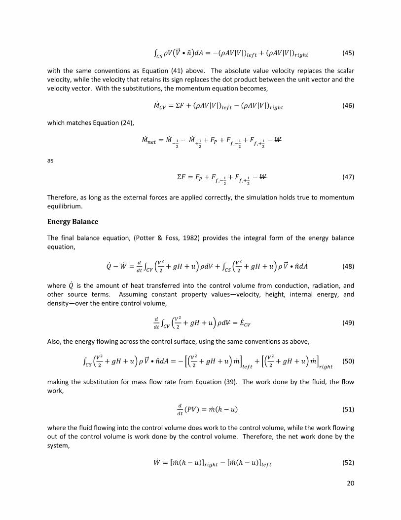
c ��_�vw • ]s`d�rt = −(���|�|)xWOX + (���|�|)yz{-X (45)

with the same conventions as Equation (41) above. The absolute value velocity replaces the scalar

velocity, while the velocity that retains its sign replaces the dot product between the unit vector and the

velocity vector. With the substitutions, the momentum equation becomes,

�� r� = ΣQ + (���|�|)xWOX − (���|�|)yz{-X (46)

which matches Equation (24),

��VWX = �� =�� −�� �� + Q + QO,=�� + QO,�� −[

as

ΣQ = Q + QO,=�� + QO,�� −[ (47)

Therefore, as long as the external forces are applied correctly, the simulation holds true to momentum

equilibrium.

Energy Balance

The final balance equation, (Potter & Foss, 1982) provides the integral form of the energy balance

equation,

�� −[� = qqXc f�� + �� + �g�d�r� + c f�� + �� + �g�rt �vw • ]sd� (48)

where �� is the amount of heat transferred into the control volume from conduction, radiation, and

other source terms. Assuming constant property values—velocity, height, internal energy, and

density—over the entire control volume,

qqX c f�� + �� + �g�d�r� = $�r� (49)

Also, the energy flowing across the control surface, using the same conventions as above,

c f�� + �� + �g�rt �vw • ]sd� = − �f�� + �� + �g�� �xWOX + �f�� + �� + �g�� �yz{-X (50)

making the substitution for mass flow rate from Equation (39). The work done by the fluid, the flow

work,

qqX (��) = �� (ℎ − �) (51)

where the fluid flowing into the control volume does work to the control volume, while the work flowing

out of the control volume is work done by the control volume. Therefore, the net work done by the

system,

[� = '�� (ℎ − �)(yz{-X − '�� (ℎ − �)(xWOX (52)

21

The current state of the simulation neglects heat transfer, so Equation (48) becomes,

$�r� = �f�� + �� + ℎg�� �xWOX − �f�� + �� + ℎg�� �yz{-X (53)

which matches Equation (20),

$�VWX = $�=�� −$���

showing that the simulation matches the energy conservation equation as well.

The simulation obeying all three continuity equations supports the idea that it accurately models real

fluid cases. Further support exists in the validation section found later in this thesis, where results of the

simulation are compared to expected results from various flow models.

22

Two-Phase Model

Like the single phase model, the two phase simulation employs alternating junction and volume blocks

which base their calculations on the mass, momentum, and energy held in the volume blocks, the

independent variables of the system. Both blocks perform the same basic functions as their single phase

counterparts; the junction block calculates the flow rates of mass, momentum, and energy, while the

volume block integrates the flow rates over time to find the state of the fluids.

Because of the liquid and gas phases, each junction block is divided into two parts, one to calculate the

flow rates for each phase. The gas section executes first, following a process similar to the single-phase

junction block. The pressure is determined by the gas alone, so the liquid section must run after, using

the average gas pressure in the momentum flow calculation. Instead of sending one set of flow rates to

adjacent volume blocks, the junction block sends the mass, momentum, and energy flow rates

separately for each phase.

The volume block also differs from the single phase model, incorporating the interactions between the

two phases. Before the volume block integrates the energy flows, the energy rate of change adjusts for

each flow based on the temperature difference between the phases. Likewise, because of interphase

drag, the momentum flow for each phase changes based on the velocity difference. The energy and

momentum transfers include adjustable coefficients: the interphase heat transfer coefficient and the

interphase friction factor. Though the fluids exchange momentum and energy, they do not exchange

mass; phase change is not yet incorporated into the simulation.

Also, because the gas phase does not occupy all of the space within the volume block, the state

calculations following the flow integrations differ in the two phase model. First, the state of the liquid is

found. The density of the liquid remains constant; in addition to the state of the liquid, the volume

block calculates the space occupied by the liquid, using the constant density and the current mass of

liquid. The remaining volume the gas phase occupies. The state of the gas is now able to be found,

given the adjusted volume.

Junction Calculations

The previous section gave a brief overview on the differences between the single phase and two phase

models. This junction calculations section, and the following volume calculations section, will explain

the operation of the two phase simulation in detail.

As with the single phase simulation, the two phase junction block uses Equation (1) to find the average

temperature, density, and velocity for both the liquid and gas phases. Junctions with only adjacent

volume block use the extrapolating Equation (36) to find the same properties. The junction block also

length averages (or extrapolates) void fraction, defined as

� ≡ ��� (54)

where the subscripts � and refer to the gas and liquid phases, is the volume occupied by the gas

phase. With the state of the gas phase known, Equation (2), the equation of state for an ideal gas, is

used to find gas pressure. Assuming that the gas phase drives the pressure, the junction pressure,

23

� = �� = �� (55)

so that the same pressure is used for both phases, and the overall junction pressure.

Because the perimeter of pipe is assumed to be wetted, wall friction affects the liquid phase only.

Various models have been proposed that derive a smooth pipe friction factor, but none are used in this

simulation. Equations (17) and (18) are used with the liquid phase properties to determine the force of

friction on the liquid phase.

To calculate the mass, momentum and energy flows for each phase, Equations (3), (4), and (11) are used

with one small adjustment; the cross-sectional area for each phase is not full cross-sectional area of the

pipe and must be calculated using void fraction. The junction finds the length-weighted average of void

fraction using Equation (1), as with the other state variables. Therefore, the mass flow of gas,

�� � = ������ (56)

and liquid,

�� � = ��(1 − �)��� (57)

Using the new values for mass flow, the simulation finds the momentum flow rates for gas,

��� ≡ �� ��� (58)

and liquid,

�� � ≡ �� ��� (59)

as well as energy flow rates for gas,

$�� = �� �(��� + "�,��� + !�) (60)

and liquid,

$�� = �� �(�� + "�,��� + !�) (61)

For two-phase flow, Equations (56) through (61) provide the flow rates needed by the adjacent volume

blocks, explained in the following section.

24

Volume Calculations The volume block contains the interactions between the liquid and gas phases, the primary difference

between the single phase and two phase model. The two phase volume block takes the flow rate (and

friction) information from the adjacent junction blocks as inputs. The momentum and energy flow rates

are adjusted based on the friction and heat transfer between the two phases. Pressure and wall friction

alter the momentum flow rates as well. The adjusted flow rates are integrated to find the current

values of mass, momentum and energy within the cell. Finally the amount of mass, momentum and

energy (of each phase) determine the state of the fluids, including void fraction.

Weight

Like Equation (23), a weight is applied to the fluids in the pipe; however, the two phase simulation uses

a separate equation for each phase. In each volume, the gas phase weighs,

[� = ����� • @\](^) (62)

and the liquid phase weighs,

[� = ��(1 − �)�� • @\](^) (63)

The weights are applied in the momentum balance equations, where the gas momentum balance

includes [�, and the liquid balance equation includes [�.

Pressure Balance

In the single phase model, pressure applies a force on the inlet and outlet of each volume block. Also, if

the area changes from one end to the other, the pressure force normal to the wall of the pipe has a

component in the flow dimension. The simulation calculates this pressure balance using Equation (22).

Similarly, the two phase model balances inlet, outlet, and wall pressures; however, this balance occurs

for each phase. The inlet and outlet areas change based on the void fractions in the neighboring

junctions. The gas boundary area,

��, = �� (64)

and the liquid boundary area,

��, = (1 − �)� (65)

where the properties are taken from adjacent volumes. Applying Equation (22) to the two phases yields

the pressure forces,

Q ,� = (���)=�� − (���)�� + � Y�=�� + ���Z Y���� − ��=��Z (66)

for the gas phase, and

Q ,� = (���)=�� − (���)�� + � Y�=�� + ���Z Y���� − ��=��Z (67)

for the liquid phase. Equations (66) and (67) are included in the momentum balances to follow.

25

Interphase Drag Momentum Transfer

The interphase momentum transfer is driven by the velocity difference between the two phases. If the

two fluids move at different velocities, a drag force appears, acting against the greater velocity fluid and

with the lower velocity fluid. The interphase velocity difference,

Δ�z� = �� − �� (68)

where the subscript \� refers to “interphase”. The simulation uses the velocity difference to calculate

the drag force included in the momentum balance equations,

,z� = �)* Az��(1 − �)��Δ�z� (69)

Please note that the sign of ,z� is the same as the sign of Δ�z�, so that force is always applied to the

lower velocity fluid in the positive direction. Equation (69) crudely represents interphase drag; more

sophisticated models exist, but there is no consensus on the exact mechanisms of interphase drag. This

model of interphase drag prevents one phase—namely the gas, wall friction does not affect the gas

phase—from travelling at a velocity much higher than the other. The product �(1 − �) reduces drag for

high and low void fractions, when there is less interphase area, increasing stability for those cases.

Interphase Drag Energy Dissipation

Interphase drag not only transfers momentum between phases, but involves the phases performing

work on one another. The time-derivative work term is power,

[� = qqX ([) = qqX (Qd) = Q� (70)

where [ is work. Since both phases are moving and applying a force to one another, Equation (70)

shows the power each phase exerts on the other. The gas phase applies

[� �→� = ,z��� (71)

to the liquid phase, while the liquid phase applies

[� �→� = −,z��� (72)

to the gas phase, where the subscripts � → and → � describe the source and sink of the power.

Notice that Equation (72) is negative. Drag force shares its sign with velocity difference, which is

positive if the gas velocity is greater. By this convention, drag force is applied in the negative direction

on the gas phase and in the positive direction on the liquid phase. Therefore the power applied on the

gas phase, Equation (72), must be negative.

Because the fluid velocities are not necessarily the same,

[� �→� ≠ −[� �→� (73)

and some of the work due to interphase friction is dissipated. The dissipated power,

[� qzN� = [� �→� +[� �→� (74)

26

which represents the kinetic energy lost by the gas phase, but not gained by the liquid phase. This

dissipated is assumed to split evenly between the two phases, such that,

[� VWX,� = �� ��T� −[� �→� (75)

and

[� VWX,� = �� ��T� +[� �→� (76)

No energy is destroyed, and using the Equations (71) through (76), the interphase power due to friction,

[� z� = [� VWX,� = −[� VWX,� = � (�� + ��),z� (77)

which is added to the liquid energy balance and subtracted from the gas energy balance. In reality, this

dissipation may not be evenly distributed between the phases, but splitting the dissipation is a closer

approximation that one phase taking all of the dissipated energy, which would occur without this

correction term. Regardless, interphase heat transfer dominates the flow of energy from one phase to

the other.

Expansion Work

An additional work term exists between the two phases. If the volumes of each phase change over time,

then the expanding volume performs work on the contracting volume. The pressure of each phase is

assumed to be equal, while the volumes are not necessarily equal. Therefore, the power done on the

gas phase by the liquid phase,

[� W���V,� = � q��qX (78)

and the power done by the gas phase on the liquid phase,

[� W���V,� = � q��qX (79)

Because the liquid phase gains any volume lost by the gas phase,

q��qX = − q��qX (80)

and, because the density of liquid is assumed constant, the liquid mass rate of change determines the

liquid volume rate of change,

q��qX = h� ���,�!� (81)

So the net work due to expansion,

[� W���V,VWX = �h� ���,�!� (82)

which is added to the gas phase energy balance, and subtracted from the liquid phase energy balance.

27

Interphase Heat Transfer

The final interphase transfer term is the heat transfer between the two phases. The temperature

difference between the phases,

Δ�z� = �� − �� (83)

drives the flow of heat from one phase to the other. The interphase heat transfer rate per unit volume,

��z� = ℎΔ�z��(1 − �)� (84)

where ℎz� is the volumetric heat transfer coefficient, in � �h�=��. Equation (84) is a simple formulation

based on convective heat transfer. Again, similar to the interphase friction model, Equation (69), the

term �(1 − �) represents the reduction in interphase area as void fraction approaches 1 or 0. Reducing

heat transfer in these cases prevents too much heat being transferred to a phase with significantly less

mass, improving stability in those cases.

Balance Equations

Like Equation (19), the mass balance for the two phase model only includes the inlet and outlet flows.

For the two phase simulation, the difference is the separate balance for each phase. Equation (19)

becomes

�� VWX,� = �� =��,� −�� ��,� (85)

for the ideal gas phase, and

�� VWX,� = �� =��,� −�� ��,� (86)

for the incompressible liquid phase, with the gas and liquid junction mass flow terms defined by

Equations (56) and (57), respectively.

Compared to the one-phase energy balance equation, Equation (20), the two phase energy balance

contains additional terms, the frictional work, expansion work, and interphase heat transfer. For the

liquid phase, the rate of change of energy,

$�VWX,� = $�=��,� −$���,� + ��z� +[� z� +[� W���V,VWX (87)

while for the gas phase,

$�VWX,� = $�=��,� −$���,� − ��z� −[� z� −[� W���V,VWX (88)

The signs on the work and heat transfer terms change between Equations (87) and (88) because those

terms transfer energy from one phase to the other.

28

The momentum balance also includes an additional term compared to the single phase counterpart,

Equation (24). Interphase drag transfers momentum from one phase to the other. The resulting

momentum rate of change for liquid,

��VWX,� = �� =��,� −�� ��,� + Q ,� + QO,=�� + QO,�� −[� + ,z� (89)

and gas,

��VWX,� = �� =��,� −�� ��,� + Q ,� −[� − ,z� (90)

Like in the energy equations, the transfer term ,z� has a different sign in Equations (89) and (90),

representing the transfer of momentum from one phase to the other due to interphase friction. Also,

Equation (90) does not contain frictional terms, as the liquid phase is the only phase that contacts the

wall of the pipe.

With all six rates of change known (�� VWX,� ,�� VWX,� , $�VWX,�, $�VWX,� ,�� VWX,�,�� VWX,�), the two phase model

employs the same integration procedure as the single phase model, Equation (25). The integration

results in knowing the total mass, momentum, and energy of each phase within the cell.

Equations of State

The volume begins calculating values to be used by adjacent junction blocks. First, void fraction must be

found. Knowing that the mass of liquid,

�� = ���� = ��(1 − �)� (91)

and that the density of the liquid does not change, the volume’s void fraction,

� = 1 − h�!�� (92)

As the gas density varies, the volume calculates it at each time step. The density of gas,

�� = h��� = h��� (93)

The remaining properties, velocity and temperature, are calculated using Equations (32) and (33), except

that the volume block finds a different temperature and velocity for each phase.

As with the single phase model, the two phase model passes the flow rate information from the junction

blocks to the volume blocks. The volume blocks use this information to determine the states of the

fluids in the next time step. The gas and liquid states are given to the junction blocks, which use them to

calculate the flow rate information, thus perpetuating the cycle.

29

Relation to Balance Equations The equations presented in (Ishii & Takashi, 2011) provide a standard of comparison for the two-phase,

one-dimensional flow simulation developed in this thesis. The following sections show that, using the

assumptions employed by the model, each balance equation simplifies to the governing equation of the

simulation.

Mass Continuity

The work of (Ishii & Takashi, 2011) provides the mass balance equation in rectangular coordinates,

��X (�� �̅̅�) + ��� (�� �̅̅��s��) + ��� _�� �̅̅��s��` + ��p (�� �̅̅��sp�) = Γ� (94)

where à is the mass generation term, the subscript � specifies to which fluid the property belongs, ��

refers to the volume fraction of fluid-�, not necessarily the void fraction, the subscripts �, �, and o refer

to the axis the vector component lies on, the hat, ̂ , indicates the property is a mass-weighted mean,

and the double-bar, ̅ ̅ , indicates the property is a mean value. As a one-dimensional model only

considers one axis of fluid flow, Equation (94) reduces to

qqX (�� �̅̅�) + qq� (�� �̅̅��s�) = Γ� (95)

where all fluid velocity occurs in the x-direction. Also, the model cannot currently model phase change;

Equation (95) further reduces to

qqX (�� �̅̅�) + qq� (�� �̅̅��s�) = 0 (96)

which, after multiplying all terms by the volume of the volume block (the control volume), yields

� � qqX (�� �̅̅�)� + � � qq� (�� �̅̅��s�)� = �� � + � qq� (�� �̅̅��s�) = 0 (97)

Setting the differential length equal to the length of the control volume,

�� � + �¡(�� �̅̅��s�)yz{-X − (�� �̅̅��s�)xWOX¢ = 0 (98)

where the distance between the left and right boundary is the length of the control volume. Now, to

apply the reduced mass continuity equation to the two phase simulation, it must be represented in the

gas form,

�� � = �¡(��̅̅��s�)xWOX − (��̅̅��s�)yz{-X¢ (99)

and liquid form,

�� � = �¡('1 − �(�̅̅��s�)xWOX − ('1 − �(�̅̅��s�)yz{-X¢ (100)

which matches the gas continuity, Equation (85), and liquid continuity, Equation (86), used by the

simulation, except for two differences. First, Equation (100) does not evaluate the cross-sectional area

at the control volume boundaries, but uses a constant cross-sectional area for the entire control volume.

Second, the simulation employs length-weighted averaging of fluid properties like velocity, whereas

Equation (100) utilizes mass weighted averaging. The subtle differences negligibly affect the result of

the simulation, especially if the length resolution is large enough.

30

Momentum Balance

The x-component of the momentum balance, given by (Ishii & Takashi, 2011), is

�� �̅̅� Y£�s��£a + �s�� £�s��£� + �s�� £�s��£� + �sp� £�s��£o Z =

−�� £�¤¤�£� + �� �̅̅��s�� + ¥ ££� ��_M̅̅��� + M���1 ` + ££� ��_M̅̅��� + M���1 ` + ££o ��_M̅̅p�� + Mp��1 `¦ +_�¤¤�z − �¤¤�` ��§�� + (�s��z − �s��)Γ� +�z�� − f��§�� M̅̅���z + ��§�� M̅̅���z + ��§�p M̅̅p��zg (101)

where M�� represents the a shear stress on the fluid oriented by the axis used in the first two subscripts, �s represents Gibbs free energy (acceleration due to gravity), �z� represents generalized interfacial drag,

and the subscript \ indicated the property occurs at the interface. As all motion is assumed restricted to

the x-direction, all other spatial partial derivatives are eliminated, yielding

�� �̅̅� Yd�s��da + �s�� d�s��d� Z =

−�� q ¤¤§q� + �� �̅̅��s�� + � qq���_M̅̅��� + M���1 `� + _�¤¤�z − �¤¤�` q�§q� + (�s��z − �s��)Γ� +�z�� − q�§q� M̅̅���z (102)

Some assumptions simplify Equation (102) further. Other than the pressure differential and gravity, no

work enters or exits the system, allowing the Gibbs free energy term to be replaced with the weight of

the fluid. At any given point in the system, all phases have the same pressure, so the interface pressure

difference term also reduces to zero. As no phase change occurs, there is also no momentum transfer

due to phase change. Removing these terms gives

�� �̅̅� fq s̈©§qX + �s�� q s̈©§q� g = −�� q ¤¤q� + �� �̅̅���� + � qq���_M̅̅��� + M���1 `� + �z�� − q�§q� M̅̅���z (103)

which, multiplied by the volume of the volume block (control volume), and then setting the differential

length equal to the volume block’s length, becomes

��� �̅̅� d�s��da + ��� �̅̅��s��_�s��,yz{-X − �s��,xWOX` =

−���_�¤¤yz{-X − �¤¤xWOX` + ��� �̅̅���� + � ª¡��_M̅̅��� + M���1 `¢yz{-X − ¡��_M̅̅��� + M���1 `¢xWOX« +��z�� − �M̅̅���z(��,yz{-X − ��,xWOX) (104)

and simplifies further to

�� � = �� �_�s��,xWOX − �s��,yz{-X` + ���_�¤¤xWOX − �¤¤yz{-X` −[� + ���QO + ��z�� + ��(��,xWOX − ��,yz{-X) (105)

Equation (104) becomes

31

��� = �� �_�s�,xWOX − �s�,yz{-X` + ��_�¤¤xWOX − �¤¤yz{-X` −[� + ���→� + ��(�xWOX − �yz{-X) (106)

for the gas phase, and

�� � = �� �_�s�,xWOX − �s�,yz{-X` + (1 − �)�_�¤¤xWOX − �¤¤yz{-X` −[� + ���→� − ��(�xWOX − �yz{-X) (107)

for the liquid phase matching the gas and liquid momentum equations presented in Equations (89) and

(90).

Energy Balance

(Ishii & Takashi, 2011) gives the total energy balance equation,

�� �̅̅� ,,a ¬�̂� � �s� 2 ­ �

�® • α°_±²²³ � ±³́` � ® • _��²² • µ¶³` � �� �̅̅�µ¶³ • ·¶³ � Γ°'%�̂�z � �̂�& � %µ¶³¸ � µ¶³& • µ¶³( ��z¹¤¤�zºº � �¤¤�z f��§�X � »§!²²§�g �¼¸³ • µ¶³¸ � %®�� • ¤¤ & • µ¶³¸ �[�z1 (108)

where bold variables are vectors, variables are tensors,�̂� is specific (non-kinetic) energy, ±²²³ is

mean conduction heat flux, ±³́ is the turbulent heat flux, is the stress tensor, is the interfacial

shear stress tensor, and [�z1 is the work done by fluctuations in drag forces. Restricting Equation (108)

to the x-direction yields

�� �̅̅� dda ¬�̂� � �s� 2 ­ � �� �̅̅��s� dd� ¬�̂� � �s�

2 ­ �

dd� α°_¹¤¤� � ¹�1` � dd� _���¤¤� �s�` � �� �̅̅��s��� � Γ°'%�̂�z � �̂�& � %�s�z � �s�&�s�( ��

��z¹¤¤�zºº � �¤¤�z fq�§qX � »§!²²§�g ��z��s�z � qq� %��τ¤¤ &�s�z �[�z1 (109) ���z

where all vectors and tensors have been reduced to their x-direction scalar component. The simulation

does not involve conductive heat transfer, phase change, or drag force fluctuations, simplifying the

energy balance equation to

�� �̅̅� dda ¬�̂� � �s� 2 ­ � �� �̅̅��s� dd� ¬�̂� � �s�

2 ­ �

qq� _���¤¤ �s�` � �� �̅̅��s��� � �z¹¤¤�zºº � �¤¤�z q�§qX ��z��s�z � q

q� %����� τ¤¤ &�s�z (110) ���zMultiplying the balance by the volume of the volume block (control volume), with the assumption that

the differential length equals the length of the control volume, gives

32

��� �̅̅� dda ¬�̂� � �s� 2 ­ � ��� �̅̅��s� ¾¬�̂� � �s�

2 ­yz{-X � ¬�̂� �

�s� 2 ­xWOX¿ �

� �_���¤¤ �s�`yz{-X � _��� ���¤¤ �s�`xWOX� � ��� �̅̅��s��� � ��z¹¤¤�zºº � ��¤¤�z d��da ������z��s�z � �¡%��τ¤¤ �s�z&yz{-X � %�����z τ¤¤ �s�z&xWOX¢ (111) ���z

which further reduces to

$�� =

�� � ¾¬�̂� � �s� 2 ­xWOX � ¬�̂� ��s� 2 ­yz{-X¿ � �QO��s� �[��s� � ��z¹¤¤�zºº

�[� �,W���V −[� z�,qy�{ + �¡(��τ¤¤ �s�z)xWOX − (�����z τ¤¤ �s�z)yz{-X¢ (112) ���zusing nomenclature from the Volume Calculations of the Two-Phase Model section. The new reduced

energy balance equation matches the form of Equations (87) and (88) the gas and liquid balances used

in the simulation.

33

Simulation Validation Although the simulation matches the mass, momentum, and energy balance equations, to completely

trust the model, it must be compared against analytical flow models. Analytical models typically involve

assumptions that simplify the governing equations of a model, enabling certain flow characteristics to be

calculated without running the simulation. The simulation results are compared against the analytical

calculations to verify that the simulation can accurately represent the analytic model.

Instead of an analytical model, experimental data could be used for validation; however, matching real

data involves perfectly tuning correlations—such as friction factor, or heat transfer coefficient—to the

experimental setup. An empirical validation would not confirm the accuracy of the simulation as much

as it would confirm the accuracy of the correlations used. Because the goal of this thesis is to develop

the fluid flow model, and not to develop specific correlations, validation only includes analytical models

as standards of comparison.

The single-phase simulation is validated by three analytical models: an incompressible model with

friction, an adiabatic model with friction (Fanno flow), and an isentropic model with area change. The

incompressible model assumes that density remains constant over the length of the pipe. As the

simulation uses the ideal gas law as its equation of state, the incompressible assumption only applies

when the change of density is negligible. One measure of compressibility is the Mach number,

�? = �j (113)

where " is the speed of sound in the fluid. The speed that sound travels through a fluid is calculated by

" = √��� (114)

where � is the ratio of specific heats. For Mach numbers less than 0.3, the density remains

approximately constant and the incompressible assumption applies. The incompressible model

calculates the pressure drop due to friction for a given velocity. To validate the simulation, a pressure

drop across the system is selected, the corresponding incompressible velocity is calculated, and then the

simulation velocity is compared to the expected result.

The Fanno flow analytical model also validates the simulation. Fanno flow requires the fluid to be

steady, one-dimensional, adiabatic, and constant area (Munson, Young, & Okiishi, 1998), which the

simulation satisfies. The Fanno flow assumption allows ratios to be found as functions of Mach number

for each point along the pipe. These ratios relate a property—like velocity or pressure—to the value of

that property at a choking condition, where the Mach number equals 1. For a given simulation run, the

choking conditions should remain constant for each point along the pipe once steady state is achieved.

To validate that the simulation, the simulation runs until steady state, and the analytical choking

condition is found for several points along the pipe. If the choking condition remains constant, then the

simulation is validated.

The isentropic model verifies the accuracy of the single-phase model in a similar manner to the Fanno

flow model. Like Fanno flow, involves ratios of properties to a reference condition—either stagnation or

choking—each ratio is a function of Mach number, and the simulation is validated if the reference

conditions remain constant over the length of the pipe. The isentropic model employs two assumptions

that differ from the Fanno model; area varies along the pipe and the fluid flows without friction.

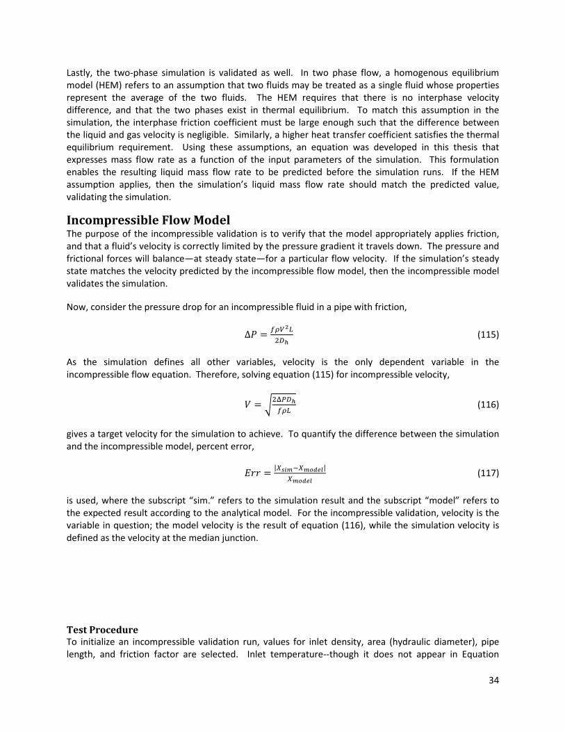
34

Lastly, the two-phase simulation is validated as well. In two phase flow, a homogenous equilibrium

model (HEM) refers to an assumption that two fluids may be treated as a single fluid whose properties

represent the average of the two fluids. The HEM requires that there is no interphase velocity

difference, and that the two phases exist in thermal equilibrium. To match this assumption in the

simulation, the interphase friction coefficient must be large enough such that the difference between

the liquid and gas velocity is negligible. Similarly, a higher heat transfer coefficient satisfies the thermal

equilibrium requirement. Using these assumptions, an equation was developed in this thesis that

expresses mass flow rate as a function of the input parameters of the simulation. This formulation

enables the resulting liquid mass flow rate to be predicted before the simulation runs. If the HEM

assumption applies, then the simulation’s liquid mass flow rate should match the predicted value,

validating the simulation.

Incompressible Flow Model The purpose of the incompressible validation is to verify that the model appropriately applies friction,

and that a fluid’s velocity is correctly limited by the pressure gradient it travels down. The pressure and

frictional forces will balance—at steady state—for a particular flow velocity. If the simulation’s steady

state matches the velocity predicted by the incompressible flow model, then the incompressible model

validates the simulation.

Now, consider the pressure drop for an incompressible fluid in a pipe with friction,

� = O!��� )* (115)

As the simulation defines all other variables, velocity is the only dependent variable in the

incompressible flow equation. Therefore, solving equation (115) for incompressible velocity,

� = 0 e )*O!� (116)

gives a target velocity for the simulation to achieve. To quantify the difference between the simulation

and the incompressible model, percent error,

$}} = |�T�Á=�ÁÂ��Ã|�ÁÂ��à (117)

is used, where the subscript “sim.” refers to the simulation result and the subscript “model” refers to

the expected result according to the analytical model. For the incompressible validation, velocity is the

variable in question; the model velocity is the result of equation (116), while the simulation velocity is

defined as the velocity at the median junction.

Test Procedure

To initialize an incompressible validation run, values for inlet density, area (hydraulic diameter), pipe

length, and friction factor are selected. Inlet temperature--though it does not appear in Equation

35

(116)—must be chosen along with exit properties to establish a pressure drop. With these independent

variables selected, Equation (116) predicts the steady state velocity of the system. To get an idea of

how well the simulation should match this value, Mach number can be predicted as well and compared

to the 0.3 rule-of-thumb.

The simulation takes the independent variables as inputs and begins simulating the system. Once the

velocity settles, the average velocity is recorded and compared to the predicted value using Equation

(117). The lower the Mach number, the lower the percent difference between predicted and simulated

should be.

To complete the validation, each independent variable should be varied in new runs. Varying the

independent variables between runs reveals any effects certain variable may have on the application of

the incompressible model. Also, analyzing more runs improves confidence in the validation result.

Table 1, in Appendix B: Simulation Data, contains the raw data used to validate the simulation’s ability

to model incompressible flow. For cases that met the incompressible assumption, inlet temperature

varied from 300 to 315 K, inlet density varied between 1.2 and 1.3 kg/m3, friction ranged from 0.05 to

0.10, area ranged from 0.01 to 0.03 m2, length remained constant at 1.66 m, and the total pressure drop

was as high as 8,600 Pa. A larger variable range for test cases was employed, but those cases did not

meet the 0.3 Mach number restriction.

Results

As expected, the error increases with increasing Mach number. For results with a Mach number less

than 0.3, the percent error does not exceed 5%, validating the simulation for low Mach numbers. Most

of the “error” present is not, in fact, a fault of the simulation, but the inability of the incompressible

model to predict velocity for an ideal gas—especially for higher Mach numbers.

To compare the agreement between the incompressible model and the simulation, the velocity results

of both are plotted against one another, as a function of Mach number. Each simulation run yields an

expected velocity (from the incompressible model) and the simulation velocity (taken from the length

midpoint of the pipe). Plotting the pair of results against Mach number shows agreement where Mach

number is less than 0.3—the incompressible region—and divergence for higher Mach numbers. Figure 9

shows the trend of increased disagreement with higher Mach numbers while Figure 10 examines the

data with less than 5% error.

As the simulation produces results that match the incompressible model’s prediction (for low Mach

numbers), the incompressible model validates the simulation. This confirms that the simulation

appropriately manages the balance between pressure drop and friction, finding the appropriate balance

between the two once steady state has been reached.

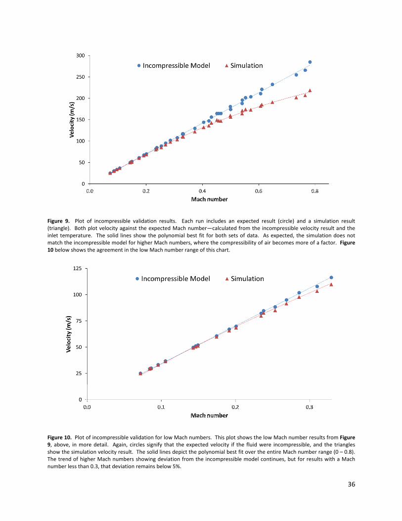
36

Figure 9. Plot of incompressible validation results. Each run includes an expected result (circle) and a simulation result

(triangle). Both plot velocity against the expected Mach number—calculated from the incompressible velocity result and the

inlet temperature. The solid lines show the polynomial best fit for both sets of data. As expected, the simulation does not

match the incompressible model for higher Mach numbers, where the compressibility of air becomes more of a factor. Figure

10 below shows the agreement in the low Mach number range of this chart.

Figure 10. Plot of incompressible validation for low Mach numbers. This plot shows the low Mach number results from Figure

9, above, in more detail. Again, circles signify that the expected velocity if the fluid were incompressible, and the triangles

show the simulation velocity result. The solid lines depict the polynomial best fit over the entire Mach number range (0 – 0.8).

The trend of higher Mach numbers showing deviation from the incompressible model continues, but for results with a Mach

number less than 0.3, that deviation remains below 5%.

37

Fanno Flow Model The purpose of the Fanno flow validation is to confirm that the simulation properly captures the

compressibility effects of an ideal gas moving through a pipe. An incompressible fluid does not

accelerate over the length of a pipe with friction, as density remains constant and mass flow rate is

constant (at steady state). For compressible fluids, with a velocity less than the speed of sound, the

velocity will increase over the length of the pipe. Fanno flow requires the flow to be steady, one-

dimensional, adiabatic, and constant area. If the simulation results match Fanno flow conditions, then

the validation confirms that the simulation models the compressible effects of an ideal gas correctly.

If Fanno flow exists, then the state at the choke point of the flow may be determined from the state at

any given point along the pipe. The ratio of a property at this arbitrary point to that property at the

choke point can be found. This includes a pressure ratio,

} = ∗ (118)

a temperature ratio,

}1 = 11∗ (119)

and a velocity ratio,

}� = ��∗ (120)

where the superscript ∗ refers to the property at choking conditions. To determine the values of the

ratios without information from the choking point, the pressure, temperature, and velocity ratios can be

found as functions of Mach number. According to (Munson, Young, & Okiishi, 1998), the pressure ratio,

} = �i� ¬ §����§��� i��­�� (121)

the temperature ratio,

}1 = §����§��� i�� (122)

and the velocity ratio,

}� = ¬ §��� i���§��� i��­

�� (123)

So, even if the simulation does not encompass the choking point, the choking properties may be found

from the state at any one simulation point.

Each simulation only has one set of choking point conditions; the choking values should not vary based

on which point was used to determine them. Therefore, to verify that the simulation can model Fanno

38

flow, the choking pressure, temperature, and velocity is found using each point of the simulation. If

these conditions remain constant, then the Fanno flow model validates the simulation.

Test Procedure

This validation of Fanno does not involve a prediction like the incompressible validation. To validate

Fanno flow, the simulation runs using any set of conditions that meet the requirements of Fanno flow.

Most notably, friction factor must be set to a non-zero constant—not using the smooth pipe correlation

of Equation (16)—and the cross-sectional area must be the same at all points along the system. All

other conditions are inherently met by the simulation.

Once the simulation reaches steady state, density, temperature, and velocity are recorded at each

junction block. Then, for each set of properties, Mach number is found, and Equations (121) through

(123) calculate the choking condition property ratios. Using the recorded state and the calculated

ratios, an estimated choking condition is found for each point. If the simulation matches Fanno flow,

the choking state should not vary between junction blocks.

A normalized standard deviation measures the consistency of these choking properties and, if low

enough, validates the simulation’s ability to model Fanno flow. The normalized standard deviation,

ÅVÆyh = Ç_�È�É`�È�ɤ¤¤¤¤¤¤ (124)

where �yWO is the calculated reference (choking) property, ̅ refers to the mean of the ten points, and Å

refers to the standard deviation of the points in the simulation. The normalized standard deviation

quantifies how much the choking properties vary between the simulation points from which they were

calculated.

A variety of different cases were simulated to validate the simulations ability to represent the Fanno

flow model. The recorded densities varied between 0.62 to 1.40 kg/m3; temperatures varied from 284

to 330 K; velocities ranged from 105 to 348 m/s; pressures ranged from 51 to 112 kPa. Without the low

Mach number restriction, a greater range of acceptable properties becomes available. The Fanno flow

validation data is available for all runs tested, available in Table 2 of Appendix B: Simulation Data.

Results

For all runs, the simulation had a normalized standard deviation around 0.01%, indicating good

agreement with the Fanno flow model. To visualize the agreement between the Fanno flow model and

the simulation results, Figure 11, Figure 12, and Figure 13 plot both against Mach number (calculated

from simulation velocity and temperature). In these figures, the hollow squares show the simulated

property ratios,

}� = ��È�ɤ¤¤¤¤¤¤ (125)

for each point of each simulation run. Equation (121) through Equation (123) are plotted on Figure 11

through Figure 13 respectively, to show the expected Fanno flow property ratio as a function of Mach

number. Deviation from the expected value is not discernible on a scale that accounts for the properties’

fluctuation along the pipe.

The agreement between the Fanno flow model and the simulation indicate that the simulation properly

accounts for the effects of a compressible gas.

39

Figure 11. Plot of Fanno flow validation, showing temperature property ratios against Mach number. The empty squares plot

the temperature at each point of each simulation, divided by the average estimated choking temperature of that simulation

run. The solid black line represents the calculated temperature ratio based on Mach number. No deviation can be seen at this

scale, and more zoomed scales yield the same conclusion. The simulation accurately models Fanno flow.

Figure 12. Plot of Fanno flow validation, showing pressure property ratios against Mach number. The empty squares plot the

pressure at each point of each simulation, divided by the average estimated choking pressure of that simulation run. The solid

black line represents the calculated pressure ratio based on Mach number. No deviation can be seen at this scale, and more

zoomed scales yield the same conclusion. The simulation accurately models Fanno flow.

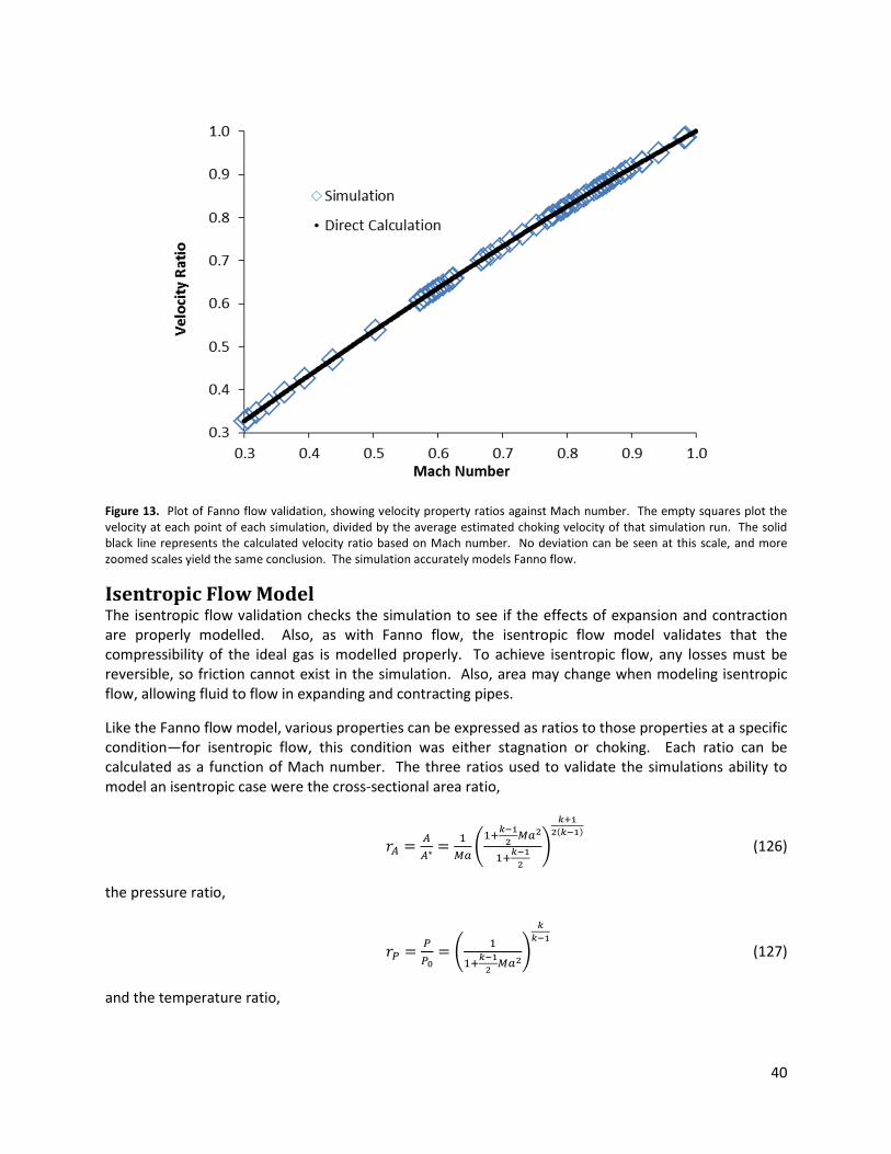
40

Figure 13. Plot of Fanno flow validation, showing velocity property ratios against Mach number. The empty squares plot the

velocity at each point of each simulation, divided by the average estimated choking velocity of that simulation run. The solid

black line represents the calculated velocity ratio based on Mach number. No deviation can be seen at this scale, and more

zoomed scales yield the same conclusion. The simulation accurately models Fanno flow.

Isentropic Flow Model The isentropic flow validation checks the simulation to see if the effects of expansion and contraction

are properly modelled. Also, as with Fanno flow, the isentropic flow model validates that the

compressibility of the ideal gas is modelled properly. To achieve isentropic flow, any losses must be

reversible, so friction cannot exist in the simulation. Also, area may change when modeling isentropic

flow, allowing fluid to flow in expanding and contracting pipes.

Like the Fanno flow model, various properties can be expressed as ratios to those properties at a specific

condition—for isentropic flow, this condition was either stagnation or choking. Each ratio can be

calculated as a function of Mach number. The three ratios used to validate the simulations ability to

model an isentropic case were the cross-sectional area ratio,

}Ê = ÊÊ∗ � �i� ¬�

§��� i���§��� ­

§���%§��& (126)

the pressure ratio,

} = 2 = ¬ ��§��� i��­§§��

(127)

and the temperature ratio,

41

}1 = 112 = ��§��� i�� (128)

according to (Munson, Young, & Okiishi, 1998). So, like the Fanno flow model, the reference properties

may be estimated from the values at any point of the simulation.

Each simulation only has one set of reference conditions; the reference values should not vary based on

which point was used to determine them. Therefore, to verify that the simulation can model isentropic

flow, the area, pressure, and temperature is found using each point of the simulation. If these

conditions remain constant, then the Fanno flow model validates the simulation.

Test Procedure

The isentropic validation procedure involves a process similar to the Fanno flow validation procedure.

Any combination of inlet and outlet conditions may be used for a validation run, and, once the

simulation reaches steady-state, the properties of interest—cross-sectional area, pressure, and

temperature—are recorded at each junction block. Then, in a manner similar to the Fanno flow

validation, Equations (126) through (128) use the recorded values and a calculated Mach number to

determine the choking cross sectional area, and the stagnation pressure and temperature. If these

reference values remain constant for all points along the pipe, the simulation accurately models

isentropic flow.

Two differences exist between Fanno flow and isentropic flow setup. The first is that no friction exists

when validating isentropic flow, as friction is an irreversible process; friction factor is set to 0 for these

runs. The second involves the cross sectional area of the pipe. Fanno flow requires that cross-sectional

area remain constant at all points for a given simulation. Isentropic allows the cross-sectional area to

change; flow expansion and contraction is a reversible process that the isentropic validation models.

The isentropic validation involves testing both contraction and expansion. Each volume block accepts an

input for cross-sectional area; for isentropic validation, these inputs must each be specified. For each

contraction case, the cross-sectional area decreases for each successive downstream volume block.

Likewise, expanding sections require the cross-sectional area to increase for each successive block.

The contracting sections provide resistance to flow, as the flow area decreases. The area difference

term in Equation (22) shows that a decreasing area creates a force opposite the direction of flow. This

flow-resisting force enables the simulation to reach steady-state, a substitute for the flow-resisting

friction force not allowed in an isentropic model. The expanding sections, however, cannot run stably

on its own because of the opposite effect; the area change yields a force in the direction of flow,

perpetuating instability. To counteract the instability, a contraction was added to the expansion cases.

Thus, the simulation included a net area reduction—net force against flow—while still having expansion

to validate the simulation’s ability to model expanding flow.

In Appendix B: Simulation Data, Table 3 shows the isentropic validation results for a contracting pipe

section. The results for an expanding-contracting pipe section are contained in Table 4 through Table 7.

Again, like the Fanno flow validation, a large range of flow properties were tested to ensure the validity

of the simulation’s ability to model isentropic flow. Cross-sectional areas ranged from 0.02 to 0.04 m2;

temperatures varied from 300 to 400 K; densities ranged from 0.95 to 1.25 kg/m3; pressures fluctuated

between 82 and 145 kPa; Mach numbers covered the range from 0.12 to 0.97.

42

Results

The results demonstrate that the simulation matched the isentropic model as the normalized

deviation—using Equation (124)—remaining below 2% for the contraction validation cases. In Figure 14

through Figure 17, the property ratios—area over choking area, pressure over stagnation pressure, and

temperature over stagnation temperature—are plotted against Mach number. The solid line in these

figures show the result of Equations (126) through (128), the analytical ratios based on Mach number.

The empty squares show the ratios derived from the simulation, using Equation (125).

Compared to the Fanno flow validation, some visible deviation from the analytical model exists.

However, this deviation is small; as seen in Figure 14 through Figure 17, the difference between the

simulation and analytical results is not significant, when compared to the entire range of data. Please

note that Figure 15 shows the same data as Figure 14, except on a smaller scale so the deviation may be

visible.

The expansion-contraction validation surprisingly resulted in a slightly better match between the

simulation and analytical results, with normalized deviation less than 1% for all points. As seen in Figure

18 through Figure 20, when the expansion-contraction results are compared to the analytical expected

values, little deviation can be seen. These plots were made using the same method as the contraction

validation plots.

With good agreement between the analytical and simulation results, the isentropic model validates the

accuracy of the simulation. This confirms the simulation’s ability to model the effect of expansion and

contraction on an ideal gas. The mismatches do require future study; the deviation may originate from

the extrapolation of boundary junction volumes or the resolution of the model.

Figure 14. Plot of contraction isentropic validation, showing cross-sectional area ratios against Mach number. The empty

squares plot the area at each point of each simulation, divided by the average estimated choking temperature of that

simulation run. The solid black line represents the calculated area ratio based on Mach number. No deviation can be seen at

this scale, but zooming reveals variation on a smaller scale, as seen in Figure 15. This variation is minimal, so the simulation

accurately models isentropic flow.

43

Figure 15. Plot of contraction isentropic validation, showing cross-sectional area ratios on a smaller Mach number range. The

empty squares plot the area at each point of each simulation, divided by the average estimated choking area of that simulation

run. The solid black line represents the calculated area ratio based on Mach number. This scale reveals variation, as it is a

subset of the data shown in Figure 14. This variation is minimal—considering the range—so the simulation accurately models

isentropic flow.

Figure 16. Plot of contraction isentropic validation, showing pressure ratios against Mach number. The empty squares plot the

pressure at each point of each simulation, divided by the average estimated stagnation pressure of that simulation run. The

solid black line represents the calculated pressure ratio based on Mach number. Some deviation can be seen at this scale;

however, this variation is minimal, so the simulation accurately models isentropic flow.

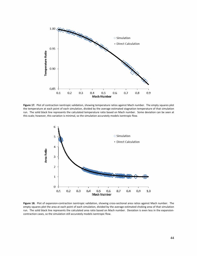
44

Figure 17. Plot of contraction isentropic validation, showing temperature ratios against Mach number. The empty squares plot

the temperature at each point of each simulation, divided by the average estimated stagnation temperature of that simulation

run. The solid black line represents the calculated temperature ratio based on Mach number. Some deviation can be seen at

this scale; however, this variation is minimal, so the simulation accurately models isentropic flow.

Figure 18. Plot of expansion-contraction isentropic validation, showing cross-sectional area ratios against Mach number. The

empty squares plot the area at each point of each simulation, divided by the average estimated choking area of that simulation

run. The solid black line represents the calculated area ratio based on Mach number. Deviation is even less in the expansion-

contraction cases, so the simulation still accurately models isentropic flow.

45

Figure 19. Plot of expansion-contraction isentropic validation, showing pressure ratios against Mach number. The empty

squares plot the pressure at each point of each simulation, divided by the average estimated stagnation pressure of that

simulation run. The solid black line represents the calculated pressure ratio based on Mach number. Deviation is even less in

the expansion-contraction cases, so the simulation still accurately models isentropic flow.

Figure 20. Plot of expansion-contraction isentropic validation, showing temperature ratios against Mach number. The empty

squares plot the temperature at each point of each simulation, divided by the average estimated stagnation temperature of

that simulation run. The solid black line represents the calculated temperature ratio based on Mach number. Deviation is even

less in the expansion-contraction cases, so the simulation still accurately models isentropic flow.

46

Two-Phase Validation

Homogeneous Equilibrium Model To validate the two phase simulation, a model must be developed—a homogeneous equilibrium model

(HEM) simplifies calculations. The HEM assumes that there is no interphase velocity difference, and that

the two phases exist in thermal equilibrium. To match this assumption in the simulation, the interphase

friction coefficient must be large enough such that the difference between the liquid and gas velocity is

negligible. Similarly, a higher heat transfer coefficient satisfies the thermal equilibrium requirement.

Successfully validating the simulation against the HEM demonstrates that the two phases correctly

interact with one another when their temperatures and velocities are nearly equal. One interaction

validated is the liquid phase occupying space that was, in the single phase model, only occupied by the

gas phase, reducing the available volume for the gas phase’s equation of state calculations. The transfer

mechanisms—interphase drag and heat transfer—are not addressed in this validation, their only

function is to balance the fluids to reach the HEM assumptions. Future work (with more sophisticated

interphase drag and heat transfer models) will require additional two-phase validations.

Developing the Validation Criterion

The pressure drop across the pipe drives the flow of liquid and gas from a high pressure to low pressure.

Working against this pressure drop is the force of friction, which only applies to the liquid phase. Steady

state occurs when these opposing force balance one another out. Modifying Equation (115), the

differential pressure change per unit length of pipe,

q q� = − O!���� )* (129)

where all properties are based on the liquid phase. To solve Equation (129), all variables must either be

a constant or a function of pressure. Solving Equation (57) for velocity yields,

�� = h� �Ê(�=�)!� (130)

and Equation (129) becomes,

q q� = =r�(�=�)� (131)

where,

#� = Oh� �� �)*!� (132)

which is a constant for a given simulation run. #� represents a pressure over length and its components

do not vary with pressure, so it may be joined together as a constant to ease the integration that

follows. Void fraction, however, varies with pressure, and must be substituted. Related to void fraction

is flow quality,

� = h� �h� �h� � (133)

or, using Equations (56) and (57),

47

� = '!�Ê���('!�Ê(�=�)��('!�Ê���( (134)

which may be simplified using the HEM assumption,

�� = �� (135)

to

� = !��!�(�=�)!�� (136)

or

1 − � = !k!k!� ©��© (137)

Substituting Equation (137) into Equation (131) yields,

q q� = −#� f!k!� ©��©g�!k� (138)

Vapor density is a function of pressure. Applying the ideal gas law,

�� = Ë1 (139)

yields,

q q� = −#� ( r�)� � (140)

where,

# = ���� ��=� (141)

which is a constant with units of pressure. Note that temperature remains approximately constant

throughout the simulation because: (1) the HEM assumes that the liquid and gas phases have the same

temperature; and (2) the high heat capacity of the liquid phase prevents much temperature change over

the length of the pipe. Therefore, # remains essentially constant with respect to pressure, and

simplifies the following integration.

Now, with Equation (140) in terms of pressure, it may be integrated,

c d� = − �r� c �( r�)� d� (142)

over the length of the pipe, such that,

� − �� = − �r� �� + # − 2# ln%� � # & � r�� r�� %��& %��& (143)

where �� and � refer to the inlet and exit positions of the pipe. Defining the inlet and exit pressures as �� and � , the integration result yields,

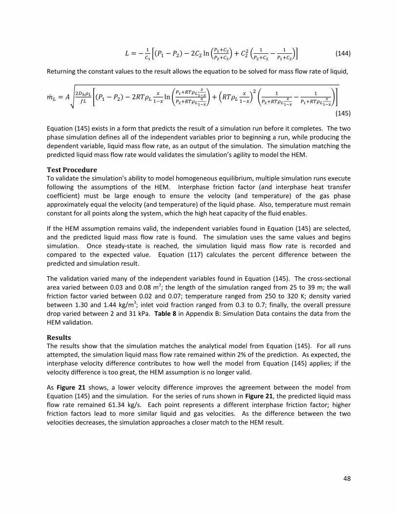
48

= − �r� �(�� − � ) − 2# ln f �r� �r�g � # f � �r� � �

�r�g� (144)

Returning the constant values to the result allows the equation to be solved for mass flow rate of liquid,

�� � = �Î )*!�O� Ï(�� − � ) − 2���� ��=� ln ¬ �Ë1!�

©��© �Ë1!� ©��©­ � f���� �

�=�g ¬ � �Ë1!� ©��©

� � �Ë1!� ©��©

­Ð (145)

Equation (145) exists in a form that predicts the result of a simulation run before it completes. The two

phase simulation defines all of the independent variables prior to beginning a run, while producing the

dependent variable, liquid mass flow rate, as an output of the simulation. The simulation matching the

predicted liquid mass flow rate would validates the simulation’s agility to model the HEM.

Test Procedure

To validate the simulation’s ability to model homogeneous equilibrium, multiple simulation runs execute

following the assumptions of the HEM. Interphase friction factor (and interphase heat transfer

coefficient) must be large enough to ensure the velocity (and temperature) of the gas phase

approximately equal the velocity (and temperature) of the liquid phase. Also, temperature must remain

constant for all points along the system, which the high heat capacity of the fluid enables.

If the HEM assumption remains valid, the independent variables found in Equation (145) are selected,

and the predicted liquid mass flow rate is found. The simulation uses the same values and begins

simulation. Once steady-state is reached, the simulation liquid mass flow rate is recorded and

compared to the expected value. Equation (117) calculates the percent difference between the

predicted and simulation result.

The validation varied many of the independent variables found in Equation (145). The cross-sectional

area varied between 0.03 and 0.08 m2; the length of the simulation ranged from 25 to 39 m; the wall

friction factor varied between 0.02 and 0.07; temperature ranged from 250 to 320 K; density varied

between 1.30 and 1.44 kg/m3; inlet void fraction ranged from 0.3 to 0.7; finally, the overall pressure

drop varied between 2 and 31 kPa. Table 8 in Appendix B: Simulation Data contains the data from the

HEM validation.

Results

The results show that the simulation matches the analytical model from Equation (145). For all runs

attempted, the simulation liquid mass flow rate remained within 2% of the prediction. As expected, the

interphase velocity difference contributes to how well the model from Equation (145) applies; if the

velocity difference is too great, the HEM assumption is no longer valid.

As Figure 21 shows, a lower velocity difference improves the agreement between the model from

Equation (145) and the simulation. For the series of runs shown in Figure 21, the predicted liquid mass

flow rate remained 61.34 kg/s. Each point represents a different interphase friction factor; higher

friction factors lead to more similar liquid and gas velocities. As the difference between the two

velocities decreases, the simulation approaches a closer match to the HEM result.

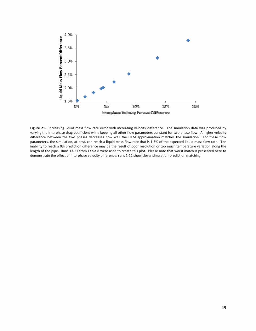
49

Figure 21. Increasing liquid mass flow rate error with increasing velocity difference. The simulation data was produced by

varying the interphase drag coefficient while keeping all other flow parameters constant for two phase flow. A higher velocity

difference between the two phases decreases how well the HEM approximation matches the simulation. For these flow

parameters, the simulation, at best, can reach a liquid mass flow rate that is 1.5% of the expected liquid mass flow rate. The

inability to reach a 0% prediction difference may be the result of poor resolution or too much temperature variation along the

length of the pipe. Runs 13-21 from Table 8 were used to create this plot. Please note that worst match is presented here to

demonstrate the effect of interphase velocity difference; runs 1-12 show closer simulation-prediction matching.

50

Conclusions

Comparison to Previous Work

This section examines the work done by others related to one-dimensional flow modeling and highlights

the differences between other literature and this thesis project.

Others have used Simulink to model one-dimensional fluid flow. (Alamian, Behbahani-Nejad, &

Ghanbarzadeh, 2012) developed Simulink functions to model the transportation of natural gas through

pipelines. Their model does not include an energy conservation term, assuming that the flow is

isothermal. Also, Alamian’s simulation uses transfer functions in s-space to solve flow conditions.

Alamian references (Herrán-González, De La Cruz, De Andrés-Toro, & Risco-Martín, 2009), who also built

a Simulink library for analyzing gas distribution pipelines. Herrán-González also assumes isothermal

conditions, but makes no menthion of s-space or Laplace transforms.

Similar to the simulation described in this thesis, (Davis & Campbell, 2007) employs a one-dimensional

fluid flow model using mass, momentum, and energy continuity equations in their simulation. Rather

than utilizing the ideal-gas law, Davis utilizes the REFPROP database (from the National Institute for

Standards and Testing) to find the values of state variables for real fluids (as well as two-phase

mixtures). Davis’s two-phase simulation appears limited to homogeneous equilibrium (modeled as a

single fluid with a single equation of state), while the simulation featured in this thesis incorporates two-

phase flow by using the mass, momentum, and energy continuity equations separately on each phase.

Also, at the time of the journal article, Davis had not yet incorporated area change in their simulation,

which the simulation featured in this thesis includes.

The simulation from (Scheuerer & Scheuerer, 1992) employs a similar structure to the simulation

developed for this thesis. Scheuerer utilizes separate mass and momentum conservation equations for

each phase, where upstream and downstream flux terms originate from the average properties of the

adjacent control volumes; the simulation in this thesis performs the same process for conserving mass,

momentum and energy. Scheuerer did not include an energy conservation equation in their simulation,

the major difference from the simulation described by this thesis.

51

RELAP Comparison RELAP5-3D is a one-dimensional, two-phase simulation tool and the primary standard of comparison for

this thesis’s simulation. This section will explore the similarities and differences between RELAP and the

new simulation, using the RELAP5-3D user’s manual, (Idaho National Laboratory, 2005).

Mass Continuity

Like the new simulation, RELAP employs mass, momentum, and energy equations to simulate fluid flow.

The manual states the mass continuity equations,

qqX (���) + �Ê qq� (������) = Γ� (146)

and

qqX ('1 − �(��) + �Ê qq� ('1 − �(�����) = Γ� (147)

where Γ is the mass generation of each phase, and the other variables have been adjusted to match the

conventions of this thesis. RELAP does not typically employ mass sources or sinks, but does include

phase change, so that

Γ� = −Γ� (148)

The primary mass continuity difference between the new simulation and RELAP is that RELAP includes a

mechanism for phase change, while the new simulation cannot accurately model scenarios where phase

change occurs.

Momentum Conservation

The REALAP manual gives the momentum conservation equations as well. With variable substitutions to

account for the nomenclature in this thesis, the gas phase momentum balance is

����d��da + 12����d��

d� � ���d�d� � ���Ñ�� � %����&AË,��� + Γ��_��,z� − ��` −(�����)Az�(�� − ��) − #�(1 − �)���� �q(��=��)qX + �� q��q� − �� q��q� � (149)

and the liquid phase momentum balance is

(1 − �)���d��da + 12 %1 − �)���d��

d� =

−(1 − �)�d�d� + (1 − �)��Ñ�� − _(1 − �)���`AË,��� + Γ��_��,z� − ��`

−((1 − �)���)Az�(�� − ��) − #�(1 − �)���� �q(��=��)qX + �� q��q� − �� q��q� � (150)

where AË is RELAP’s wall friction factor, �zOis the velocity at the interface between the fluids, ��� is the

average density of both fluids, � is the sum of the body forces acting in the flow direction, and # is the

coefficient of virtual mass.

52

The new simulation does not include the 4th

term on the right side of Equations (149) and (150), as the momentum

transfer do to mass transfer does not apply when there is no phase change. Furthermore, the 6th

term on the right side is

excluded, as the new simulation neglects the effect of force due to virtual mass. Also, the 5th

term on the right side of Equation

(149) is omitted—the new simulation assumes a wetted pipe perimeter and only applies wall

friction to the liquid phase.

The wall friction term exists in a different form in the new simulation. Instead of being proportional to velocity, the new

simulation’s frictional force terms are proportional to velocity-squared. Furthermore, while RELAP includes many factors in its

body force term, the new simulation only includes the force due to gravity. The remaining terms in Equations (149)

and (150)—the momentum flow across boundaries (2nd

term on left), and the pressure differential (1st

term on the right)—exist in both RELAP and the thesis simulation.

Energy Conservation

The RELAP manual also gives the energy balance equations used in the RELAP simulation. The gas

energy equation is

qqX (�����) + �Ê qq� (��������) = −� q�qX − Ê qq� (����) + ���,� + ��z�,� + Γz�,�ℎ�# + ΓÓ,�ℎ�º + ,Ôuu� (151)

and the liquid energy equation is

qqX ('1 − �(����) + �Ê qq� ('1 − �(�������) = � q�qX − Ê qq� ('1 − �(���) + ���,� + ��z�,� + Γz�,�ℎ�# +ΓÓ,�ℎ�º +,Ôuu� (152)

where ��� is the heat transfer rate from the pipe wall to the fluid, ℎ# is the specific enthalpy associated

with bulk interface mass transfer, ℎº is the specific enthalpy associated with mass transfer at the wall,

and ,Ôuu is the energy dissipation term.

Again, the simulation of this thesis does not include phase change, so terms that involve energy transfer

due to phase change—the 5th

and 6th

terms on the right side of Equations (151) and (152)—are not

included in the new simulation. Also, the new simulation does not incorporate wall heat transfer, so the

3rd

right side term is excluded as well.

The new simulation employs a different convention for energy balance management. Rather than

include a dissipation term, which adds thermal energy as kinetic energy is lost due to friction, the new

simulation incorporates kinetic energy—and gravitational potential energy—into the energy

conservation equation. Therefore, when the velocity decreases due to friction—or the height of the

fluid increases—there is no net change in total energy. The simulation does not track thermal energy as

a separate entity; at each time step, the simulation subtracts the kinetic and potential energy—based in

the velocity and height—and the remaining energy is the thermal energy used to calculate temperature.

The new simulation includes the remaining terms, total energy rate of change (1st

term on the left),

energy flow across boundaries (2nd

term on the left), flow work due to void fraction change (1st

term on

the right), flow work due to velocity (2nd

term on the right), and interphase heat transfer (4th

term on the

right).

53

Next Steps This section contains potential ways to improve the simulation code. The basis of the two-phase, one-

dimensional simulation code already exists; any of the following features can be added without

changing the underlying structure of the code.

Accurate Interphase Models

Currently, the simulation allows for transfer of heat and momentum between the two phases. The

temperature difference between the two phases drives the flow of energy from the higher temperature

phase to the lower temperature phase. The heat transfer from Equation (84) is proportional to a heat

transfer coefficient. The coefficient, in the current simulation, is represented by a constant with no

empirical or theoretical backing; the HEM validation only required this constant to be large enough to

ensure that the gas and liquid temperatures would be approximately equal.

Also, the transfer of momentum due to friction—the interphase drag force—involves the placeholder

model shown in Equation (69). Not only is the frictional coefficient not known, but there is little

consensus on methods to determine interphase drag. The literature review of this thesis examines

several potential models that this simulation could incorporate. The placeholder interphase friction

model enables the simulation to run stably, as the gas phase velocity would increase with little bound

without friction from the liquid phase. Also, like the interphase heat transfer, the friction coefficient is

large enough so that the gas and liquid velocities are similar enough for the HEM validation.

To improve the interphase heat transfer and friction in the simulation, the placeholder models must be

replaced with theoretically—or empirically—backed models.

Validate Transients

The four validation cases performed on the simulation—incompressible, Fanno, isentropic, HEM—all

required steady state to be achieved. Though the steady state scenario has been validated, no

validation of the transient state of the system has been performed. The transient functions; the system

proceeds from an initial state to the steady state. It is not known if this transition occurs over the

proper amount of time. Also, the system’s response to an oscillating input should be examined.

Phase Change

While the current simulation allows for a two-phase mixture, it does not allow for phase change. To

incorporate phase change, a rate of vaporization would be needed. The rate of vaporization would be

incorporated into the gas mass balance,

�� �,VWX = (������)=�� − (������)�� + Õ (153)

and the liquid mass balance,

�� �,VWX = (�����'1 − �()=�� − (�����'1 − �()�� − Õ (154)

where the rate of vaporization,

Õ = A(�� , �� , �, �, �, ) (155)

With a correct mass transfer model in place of Equation (155), the current simulation allows easy

implementation of phase change, simply adding the equation’s result to the mass balance equation for

each phase. The correct mass transfer model will likely involve the heat transfer across the temperature

54

difference between each phase and the interface. If the two heat transfers do not balance, the

difference would yield phase change.

Wall Heat Transfer

Another desired feature is the generation of heat in the system. The heat would originate from the wall,

so the heat generation term would appear in the liquid energy balance,

$�VWX,� = $�=��,� −$���,� + ��z� +[� z� +[� W���V,VWX + ��� (156)

The heat generation term could either be a constant, or the term could be based on the temperature

difference between the wall and the liquid phase. Then, wall heat transfer,

��� = A(�� , ��, ℎ�, �, ) (157)

To validate the heat transfer model, Rayleigh flow would be used. Rayleigh flow requires heat transfer

into the fluid so that temperature remains constant. To run this validation, a wall temperature would be

selected, then Rayleigh flow requires the heat transfer coefficient be large enough so that the fluid

temperature matches the wall temperature at all points, making the Rayleigh flow assumption valid.

The resulting heat transfer rate would be recorded and compared to the Rayleigh flow predicted values.

Special Components

Currently, the only component the simulation can model is a straight pipe section, with the option to

vary the cross-sectional area. Adding different types of components would improve the code. A pump

would behave the same as a junction component, except that the pressure sent to the downstream

volume would be higher than the pressure sent to the upstream volume. A tee pipe section would

replace a junction, except that the tee would exchange information with three adjacent sections, rather

than two. A separator would act similar to tee, with the flow output in each branch restricted to a

certain void fraction. A valve would also replace a junction, behaving the same when open, but

preventing flow when closed. For curved pipe sections, a constant could be added to the friction in a

volume component, representing the losses associated with those components.

55

Bibliography

Alamian, R., Behbahani-Nejad, M., & Ghanbarzadeh, A. (2012, May 29). A state space model for

transient flow simulation in natural gas pipelines. Journal of Natural Gas Science and

Engineering(9), 51-59.

Anderson, D. A., Tannehill, J. C., & Pletcher, R. H. (1984). Coputational Fluid Mechanics and Heat

Transfer. New York: Hemisphere Publishing Corporation.

Collier, J. G., & Thome, J. R. (1994). Convective Boiling and Condensation (3rd ed.). New York: Oxford

University Press.

Davis, R. L., & Campbell, B. T. (2007, October). Quasi-One-Dimensional Unsteady-Flow Procedure for

Real Fluids. (C. Kaplan, Ed.) AIAA Journal, 45(10), 2422-2428.

Herrán-González, A., De La Cruz, J. M., De Andrés-Toro, B., & Risco-Martín, J. L. (2009, March). Modeling

and simulation of a gas distribution pipeline network. Applied Mathematical Modelling, 33(3),

1584-1600.

Hirsch, C. (1990). Numerical Computation of Internal and External Flows (Vol. 2: Computational Methods

for Inviscid and Viscous Flows). Chichester, West Sussex, England: John Wiley & Sons.

Idaho National Laboratory. (2005). RELAP5-3D (C) Code Manual (2.4 ed., Vols. 1: Code Structure, System

Models, and Solution Methods). Idaho Falls, Idaho.

Incropera, F. P., DeWitt, D. P., Bergman, T. L., & Lavine, A. S. (2007). Fundamentals of Heat and Mass

Transfer (6th ed.). Hoboken, NJ: John Wiley & Sons.

Ishii, M., & Takashi, H. (2011). Thermo-Fluid Dynamics of Two-Phase Flow (2nd ed.). New York: Springer

Science + Business Media.

Kays, W., Crawford, M., & Wiegand, B. (2005). Convective Heat and Mass Transfer (4th ed.). New York,

New York: McGraw-Hill.

Keenan, J. H., & Kaye, J. (1948). Gas Tables. New York: John Wiley & Sons.

Liles, D. e. (1988). TRAC-PF1/MOD1 correlations and models. Washington, D.C.: Nuclear Regulatory

Commission, Washington, DC (USA). Div. of Reactor Accident Analysis; Los Alamos National Lab.,

NM (USA).

Martinelli, R. C., & Nelson, D. B. (1948, August). Prediction of Pressure Drop During Forced-Circulation

Boiling of Water. Transactions of the American Society of Mechanical Engineers, 695-702.

Munson, B. R., Young, D. F., & Okiishi, T. H. (1998). Fundamentals of Fluid Mechanics (3rd ed.). New

York: John Wiley & Sons.

Potter, M. C., & Foss, J. M. (1982). Fluid Mechanics. Okemos, MI: Great Lakes Press, Inc.

56

Scheuerer, G., & Scheuerer, M. (1992). Two-fluid model simulation of two-phase flow problems using a

conservative finite-volume method. Forschung und Ingenieurwesen, 58(5), 128-134.

The MathWorks, Inc. (2012, September). MATLAB Mathematics. Retrieved December 6, 2013, from

MathWorks - MATLAB and Simulink for Technical Computing:

http://www.mathworks.com/help/releases/R2012b/pdf_doc/allpdf.html#matlab

Todreas, N. E., & Kazimi, M. S. (2012). Nuclear Systems (2nd ed., Vol. 1: Thermal Hydraulic

Fundamentals). Boca Raton: CRC Press.

United States Nuclear Regulatory Commission. (2012, March 29). NRC: Computer Codes. Retrieved

December 19, 2013, from NRC: Home Page: http://www.nrc.gov/about-

nrc/regulatory/research/comp-codes.html

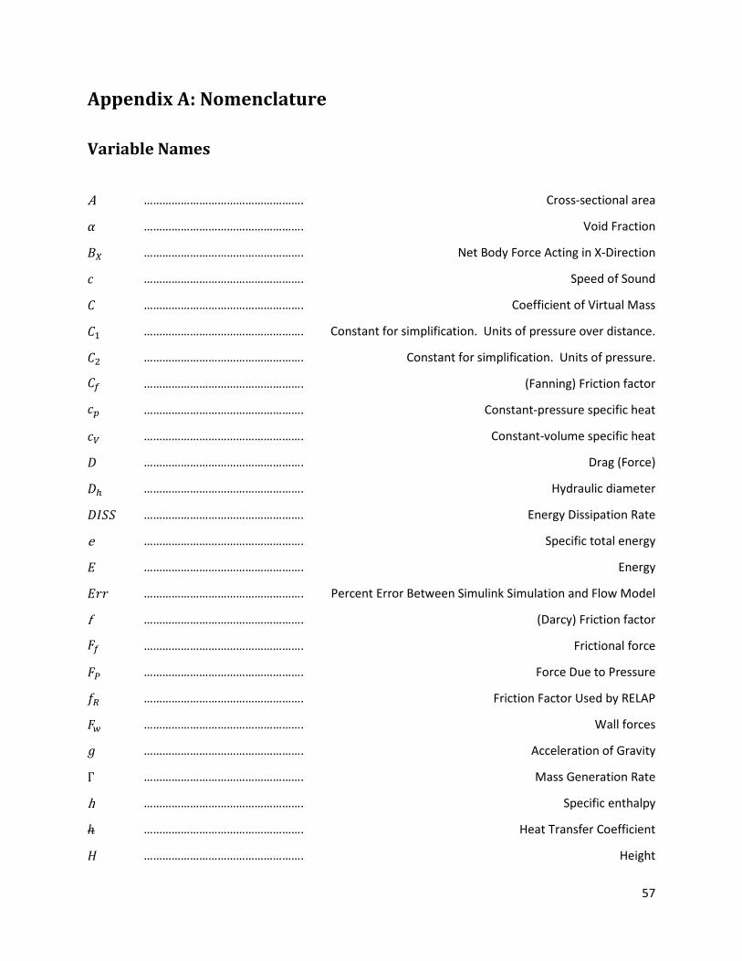
57

Appendix A: Nomenclature

Variable Names

A ……………………………………………. Cross-sectional area

� ……………………………………………. Void Fraction

Ñ� ……………………………………………. Net Body Force Acting in X-Direction

" ……………………………………………. Speed of Sound

# ……………………………………………. Coefficient of Virtual Mass

#� ……………………………………………. Constant for simplification. Units of pressure over distance.

# ……………………………………………. Constant for simplification. Units of pressure.

#O ……………………………………………. (Fanning) Friction factor

"� ……………………………………………. Constant-pressure specific heat

"� ……………………………………………. Constant-volume specific heat

, ……………………………………………. Drag (Force)

,- ……………………………………………. Hydraulic diameter

,Ôuu ……………………………………………. Energy Dissipation Rate

e ……………………………………………. Specific total energy

$ ……………………………………………. Energy

$}} ……………………………………………. Percent Error Between Simulink Simulation and Flow Model

f ……………………………………………. (Darcy) Friction factor

QO ……………………………………………. Frictional force

Q ……………………………………………. Force Due to Pressure

AË ……………………………………………. Friction Factor Used by RELAP

QÓ ……………………………………………. Wall forces

� ……………………………………………. Acceleration of Gravity

Γ ……………………………………………. Mass Generation Rate

h ……………………………………………. Specific enthalpy

ℎ ……………………………………………. Heat Transfer Coefficient

� ……………………………………………. Height

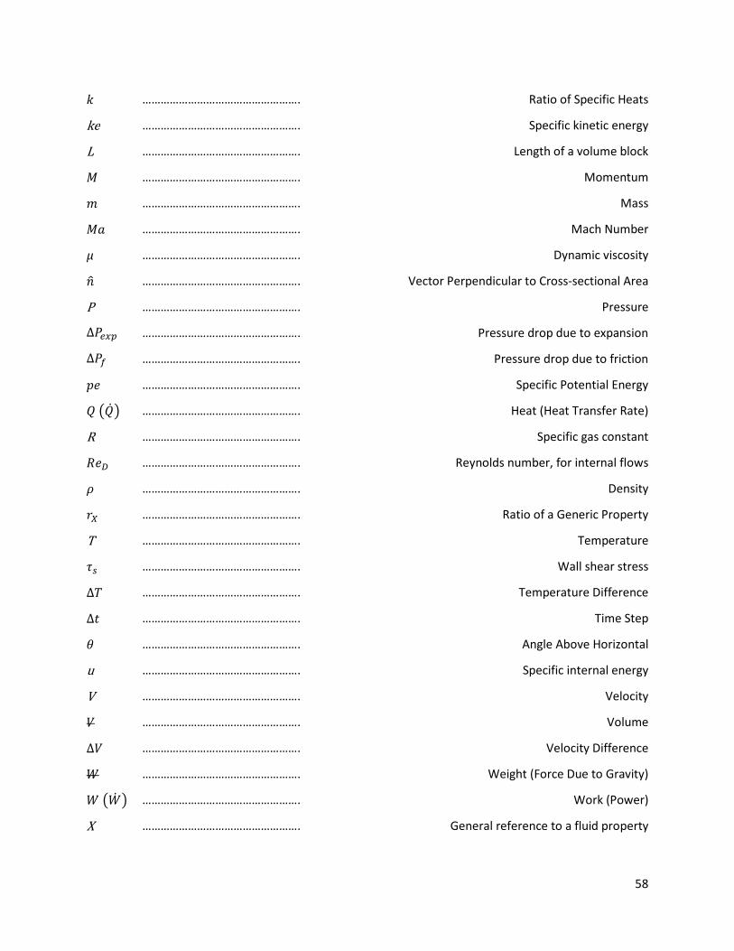
58

� ……………………………………………. Ratio of Specific Heats

ke ……………………………………………. Specific kinetic energy

L ……………………………………………. Length of a volume block

� ……………………………………………. Momentum

� ……………………………………………. Mass

�? ……………………………………………. Mach Number

. ……………………………………………. Dynamic viscosity

]s ……………………………………………. Vector Perpendicular to Cross-sectional Area

P ……………………………………………. Pressure

Δ�W�� ……………………………………………. Pressure drop due to expansion

Δ�O ……………………………………………. Pressure drop due to friction

�� ……………………………………………. Specific Potential Energy

� _�� ` ……………………………………………. Heat (Heat Transfer Rate)

R ……………………………………………. Specific gas constant

��) ……………………………………………. Reynolds number, for internal flows

� ……………………………………………. Density

}� ……………………………………………. Ratio of a Generic Property

T ……………………………………………. Temperature

MN ……………………………………………. Wall shear stress

Δ� ……………………………………………. Temperature Difference

Δa ……………………………………………. Time Step

^ ……………………………………………. Angle Above Horizontal

u ……………………………………………. Specific internal energy

V ……………………………………………. Velocity

� ……………………………………………. Volume

Δ� ……………………………………………. Velocity Difference

[ ……………………………………………. Weight (Force Due to Gravity)

[ _[� ` ……………………………………………. Work (Power)

X ……………………………………………. General reference to a fluid property

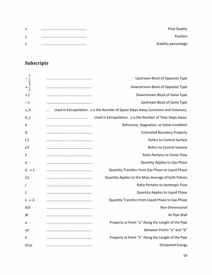
59

� ……………………………………………. Flow Quality

� ……………………………………………. Position

o ……………………………………………. Stability percentage

Subscripts

−12 ……………………………………………. Upstream Block of Opposite Type

� 12 ……………………………………………. Downstream Block of Opposite Type

�1 ……………………………………………. Downstream Block of Same Type

−1 ……………………………………………. Upstream Block of Same Type

�, 0 … Used in Extrapolation. x is the Number of Space Steps Away (Junctions and Volumes).

0, � ………………………………………. Used in Extrapolation. y is the Number of Time Steps Away.

0 ……………………………………………. Reference, Stagnation, or Initial Condition

Ñ ……………………………………………. Estimated Boundary Property

#u ……………………………………………. Refers to Control Surface

#� ……………………………………………. Refers to Control Volume

Q ……………………………………………. Ratio Pertains to Fanno Flow

� ……………………………………………. Quantity Applies to Gas Phase

� → ……………………………………………. Quantity Transfers from Gas Phase to Liquid Phase

� ……………………………………………. Quantity Applies to the Mass Average of both Pahses

Ô ……………………………………………. Ratio Pertains to Isentropic Flow

……………………………………………. Quantity Applies to Liquid Phase

→ � ……………………………………………. Quantity Transfers from Liquid Phase to Gas Phase

â, ……………………………………………. Non-Dimensional

[ ……………………………………………. At Pipe Wall

? ……………………………………………. Property at Point “a” Along the Length of the Pipe

?ã ……………………………………………. Between Points “a” and “b”

ã ……………………………………………. Property at Point “b” Along the Length of the Pipe

d\@� ……………………………………………. Dissipated Energy

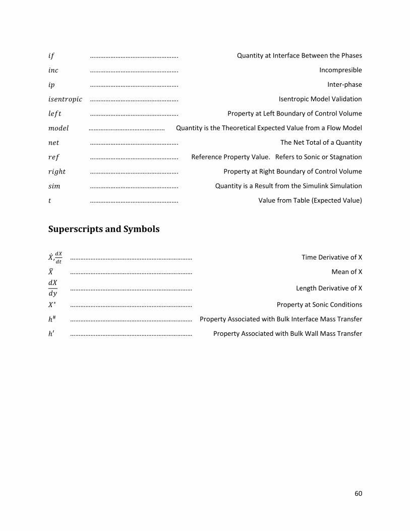
60

\A ……………………………………………. Quantity at Interface Between the Phases

\]" ……………………………………………. Incompresible

\� ……………………………………………. Inter-phase

\@�]a}ä�\" ……………………………………………. Isentropic Model Validation

|�Aa ……………………………………………. Property at Left Boundary of Control Volume

�äd�| ……………………………………… Quantity is the Theoretical Expected Value from a Flow Model

]�a ……………………………………………. The Net Total of a Quantity

}�A ……………………………………………. Reference Property Value. Refers to Sonic or Stagnation

}\�ℎa ……………………………………………. Property at Right Boundary of Control Volume

@\� ……………………………………………. Quantity is a Result from the Simulink Simulation

a ……………………………………………. Value from Table (Expected Value)

Superscripts and Symbols

�� ,q�qX ……………………………………………………………… Time Derivative of X

�¤ ……………………………………………………………… Mean of X d�d� ……………………………………………………………… Length Derivative of X

�∗ ……………………………………………………………… Property at Sonic Conditions

ℎ# ……………………………………………………………… Property Associated with Bulk Interface Mass Transfer

ℎ′ ……………………………………………………………… Property Associated with Bulk Wall Mass Transfer

61

Appendix B: Simulation Data

Incompressible Simulation The data contained in this section was used to validate that the single-phase simulation yields accurate

results while an incompressible assumption is valid. The analysis is found on page 34.

Pre-set Conditions Predictions Result

Inlet

Temperature Inlet Density

Friction

Factor Area

Total

Pressure

Drop Velocity

Average

Mach

Number

Average

Velocity

Velocity

Percent

Error

(K) (kg/m^3) (m^2) (Pa) (m/s) (m/s)

300 1.205 0.095 0.015 431 25.0 0.07 25.0 0.2%

302 1.200 0.090 0.010 689 29.4 0.08 29.4 0.3%

301 1.200 0.075 0.030 344 30.0 0.09 29.9 0.4%

302 1.200 0.070 0.010 689 33.4 0.10 33.2 0.4%

301 1.200 0.050 0.030 344 36.8 0.11 36.5 0.7%

300 1.220 0.095 0.015 1,722 49.7 0.14 49.3 0.9%

302 1.200 0.030 0.010 689 51.0 0.15 50.4 1.2%

301 1.200 0.025 0.030 344 52.0 0.15 51.2 1.5%

300 1.230 0.095 0.015 2,583 60.7 0.17 59.8 1.4%

305 1.200 0.075 0.030 1,722 67.1 0.19 65.8 2.0%

300 1.240 0.095 0.015 3,444 69.8 0.20 68.5 1.8%

305 1.200 0.050 0.030 1,722 82.2 0.23 79.7 3.1%

315 1.200 0.100 0.015 5,167 84.7 0.24 82.6 2.5%

302 1.200 0.010 0.010 689 88.3 0.25 85.0 3.8%

310 1.200 0.075 0.030 3,444 94.9 0.27 91.4 3.7%

315 1.200 0.080 0.020 5,167 101.7 0.29 97.7 3.9%

300 1.300 0.095 0.015 8,611 107.7 0.31 103.3 4.2%

310 1.200 0.050 0.030 3,444 116.3 0.33 109.6 5.7%

315 1.200 0.060 0.020 5,167 117.5 0.33 111.1 5.4%

305 1.200 0.025 0.030 1,722 116.3 0.33 109.2 6.1%

300 1.350 0.095 0.015 12,917 129.5 0.37 121.9 5.9%

315 1.200 0.040 0.020 5,167 143.9 0.40 132.1 8.2%

325 1.200 0.080 0.040 8,611 156.2 0.43 142.4 8.8%

300 1.400 0.095 0.015 17,222 146.8 0.42 135.9 7.4%

330 1.200 0.075 0.030 10,333 164.4 0.45 149.0 9.4%

320 1.200 0.050 0.030 6,889 164.4 0.46 147.3 10.4%

310 1.200 0.025 0.030 3,444 164.4 0.47 146.6 10.9%

325 1.200 0.060 0.040 8,611 180.3 0.50 159.5 11.6%

300 1.500 0.095 0.015 25,834 173.7 0.50 156.0 10.2%

325 1.300 0.060 0.015 17,940 195.7 0.54 171.1 12.6%

330 1.200 0.050 0.030 10,333 201.4 0.55 173.9 13.7%

300 1.408 0.060 0.015 17,911 187.9 0.54 164.4 12.5%

315 1.200 0.020 0.020 5,167 203.4 0.57 173.0 15.0%

325 1.200 0.040 0.040 8,611 220.9 0.61 184.9 16.3%

320 1.200 0.025 0.030 6,889 232.5 0.65 190.7 18.0%

300 1.700 0.095 0.015 43,056 210.7 0.61 181.8 13.7%

330 1.200 0.025 0.030 10,333 284.8 0.78 218.6 23.2%

300 1.700 0.065 0.015 43,056 254.7 0.73 201.6 20.9%

300 1.408 0.030 0.015 17,911 265.7 0.77 206.6 22.3%

325 1.200 0.020 0.040 8,611 312.3 0.86 229.4 26.6%

Table 1. Incompressible Validation Data. For all runs with a predicted Mach number less than 0.33, the percent difference

between the predicted velocity (from incompressible model) and the simulation average velocity remained below 5%. As the

Mach number increases, the incompressible model no longer applies. This data was created with an overall pipe length of 1.66

meters and an outlet pressure of 103,334 Pa.

62

Fanno Flow Validation The data contained in this section was used to validate that the single-phase simulation yields accurate

results while a Fanno flow assumption is valid. The analysis is found on page 37.

Table 2. Fanno Flow Validation Data. Each group of ten rows represents a single Fanno Flow validation run. Density,

temperature and velocity were recorded at ten points along the pipe for each run. Mach number was calculated, which was

then used to determine the choking condition ratios, per Equations (121) - (123). Based on these ratios, the choking

conditions were found for each point in the run. The last three columns present the variation for each of the three choking

variables in the form standard deviation divided by average of the ten points. The non-dimensional length, fL/D, did not match

as closely to the expected values.

63

Isentropic Flow Validation The data contained in this section was used to validate that the single-phase simulation yields accurate

results while an Isentropic flow assumption is valid. The analysis is found on page 40. Two sets of data

are present, the contraction case and the expansion-contraction case.

Table 3. Isentropic Flow Validation Data, Contraction. Each group of ten rows represents a single Isentropic Flow validation

run. Density, temperature, velocity, and cross-sectional area were recorded at ten points along the pipe for each run. Mach

number was calculated, which was then used to determine the choking and stagnation condition ratios, per Equations (126) -

(128). Based on these ratios, the choking conditions were found for each point in the run. The last three columns present the

variation for each of the three choking and stagnation variables in the form standard deviation divided by average of the ten

points.

64

Table 4. Isentropic Flow Validation Data, Expansion-Contraction Part 1 / 4. Each group of ten rows represents a single

Isentropic Flow validation run. Density, temperature, velocity, and cross-sectional area were recorded at ten points along the

pipe for each run. Mach number was calculated, which was then used to determine the choking and stagnation condition

ratios, per Equations (126) - (128). Based on these ratios, the choking conditions were found for each point in the run. The last

three columns present the variation for each of the three choking and stagnation variables in the form standard deviation

divided by average of the ten points. Note that the last run contains 14 points, to examine the effect of resolution on validation

results.

65

Table 5. Isentropic Flow Validation Data, Expansion-Contraction, Part 2 / 4. Each group of ten rows represents a single

Isentropic Flow validation run. Density, temperature, velocity, and cross-sectional area were recorded at ten points along the

pipe for each run. Mach number was calculated, which was then used to determine the choking and stagnation condition

ratios, per Equations (126) - (128). Based on these ratios, the choking conditions were found for each point in the run. The last

three columns present the variation for each of the three choking and stagnation variables in the form standard deviation

divided by average of the ten points. Note that the last run contains 14 points, to examine the effect of resolution on validation

results.

66

Table 6. Isentropic Flow Validation Data, Expansion-Contraction, Part 3 / 4. Each group of ten rows represents a single

Isentropic Flow validation run. Density, temperature, velocity, and cross-sectional area were recorded at ten points along the

pipe for each run. Mach number was calculated, which was then used to determine the choking and stagnation condition

ratios, per Equations (126) - (128). Based on these ratios, the choking conditions were found for each point in the run. The last

three columns present the variation for each of the three choking and stagnation variables in the form standard deviation

divided by average of the ten points. Note that the last run contains 14 points, to examine the effect of resolution on validation

results.

67

Table 7. Isentropic Flow Validation Data, Expansion-Contraction, Part 4 / 4. Each group of ten rows represents a single

Isentropic Flow validation run. Density, temperature, velocity, and cross-sectional area were recorded at ten points along the

pipe for each run. Mach number was calculated, which was then used to determine the choking and stagnation condition

ratios, per Equations (126) - (128). Based on these ratios, the choking conditions were found for each point in the run. The last

three columns present the variation for each of the three choking and stagnation variables in the form standard deviation

divided by average of the ten points. Note that the last run contains 14 points, to examine the effect of resolution on validation

results.

68

HEM Simulation Validation The data contained in this section was used to validate that the two-phase simulation yields accurate

results while an HEM assumption is valid. The analysis is found on page 46.

Table 8. HEM Validation Data. Each row represents an HEM validation run. The first group of columns show the parameters

used to set up the run. For all runs the liquid density was 1000 kg/m^3 and the outlet pressure was 101,000 Pa. The predicted

mass flow rate was calculated, before the model ran, using Equation (145). The simulation produced a liquid mass flow rate

result, once steady-state was achieved. To measure the validity of the HEM assumption, the differences in phase velocity were

also recorded. Note that runs 13-21 have the same input parameters except for interphase drag coefficient. This was to isolate

the effects of velocity difference on the variation from the expected mass flow rate value. These runs were used to create

Figure 21.

69

Appendix C: Single Phase Simulation Code

Junction Block Code

Junction_OLD function

[MassFlow,MomentumFlow,EnergyFlow,Friction,P_Ave,Ave_Vel,Ave_Rho,Ave_Temp] =

Junction_OLD(US_Temperature,US_Density,US_Velocity,US_Area,US_Length,US_Junc,

DS_Temperature,DS_Density,DS_Velocity,DS_Area,DS_Length,DS_Junc,Start,End_Pre

ssure,Last_Step,Last_2Step,US_Junc_OLD,DS_Junc_OLD,Height) %JUNCTION This is the main function to calculate the flows and state %between two adjacent volumes (or on a boundary condition). % This function finds the average temperature, pressure and velocity % between two volumes (or on a boundary condition), then calculates the % mass, momentum and energy flows between the two volumes.

%% Constants

Cv = 724.96; % [J/kg-K] R = 287.04; % [J/kg-K] expercent = 0.8; f = 0.05; % f = 0.00682613; %This constant can be adjusted to change how friction is calculated. %See the help for the function "FrictionCalc" for details.

%% Junction Type Determination

if End_Pressure > 0 %% Right Boundary Condition

A = US_Area; Total_L = 2*US_Length;

if DS_Junc.PressureForce == 9999 [Ave_Temp,Ave_Rho,Ave_Vel,P_Ave] =

Outlet_OLD(US_Temperature,US_Density,US_Velocity,DS_Temperature,DS_Density,DS

_Velocity,US_Junc,Last_Step,Last_2Step,US_Junc_OLD,expercent,R); else [Ave_Temp,Ave_Rho,Ave_Vel,P_Ave] =

Intlet_OLD(DS_Temperature,DS_Density,DS_Velocity,US_Temperature,US_Density,US

_Velocity,US_Junc,Last_Step,Last_2Step,US_Junc_OLD,expercent,R); end

elseif Start %% Left Boundary Condition

Total_L = 2*DS_Length; A = DS_Area;

if US_Junc.PressureForce == 9999

70

[Ave_Temp,Ave_Rho,Ave_Vel,P_Ave] =

Intlet_OLD(US_Temperature,US_Density,US_Velocity,DS_Temperature,DS_Density,DS

_Velocity,DS_Junc,Last_Step,Last_2Step,DS_Junc_OLD,expercent,R); else [Ave_Temp,Ave_Rho,Ave_Vel,P_Ave] =

Outlet_OLD(DS_Temperature,DS_Density,DS_Velocity,US_Temperature,US_Density,US

_Velocity,DS_Junc,Last_Step,Last_2Step,DS_Junc_OLD,expercent,R); end

else %% Interior Cells

[Ave_Temp,Ave_Rho,Ave_Vel,P_Ave,A,Total_L] =

Inner_OLD(US_Temperature,US_Density,US_Velocity,US_Area,US_Length,DS_Temperat

ure,DS_Density,DS_Velocity,DS_Area,DS_Length,R); end

%% Other Losses % These losses are added to the friction factor.

% f_adj = RapidExpansion(Ave_Vel,Ave_Rho,US_Area,DS_Area,A,Total_L,0); f_adj = 0; % P_Ave = P_Ave + 2*P_loss;

%% Flow Calculations % To be used by adjacent volumes.

[MassFlow,MomentumFlow,EnergyFlow,Friction] =

FlowPropsOLD(Ave_Temp,Ave_Rho,Ave_Vel,A,Total_L,f,f_adj,Cv,R,Height);

end

Outlet_OLD function [Ave_Temp,Ave_Rho,Ave_Vel,Ave_P] =

Outlet_OLD(IN_Temp,IN_Rho,IN_Vel,OUT_Temp,OUT_Rho,OUT_Vel,IN_Junc,Last_Step,L

ast_2Step,Adj_Junc,expercent,R) %OUTLET This function calculates the properties of a boundary condition that %is letting fluid out of the model. % This function calculates junction properties with a real volume inlet % and a constant outlet.

%Property extrapolation:

Ave_Temp =

extrapolate(IN_Temp,IN_Junc.Ave_Temp,Last_Step.Ave_Temp,Last_2Step.Ave_Temp,A

dj_Junc.Ave_Temp,IN_Temp,expercent);

71

Ave_Rho =

extrapolate(IN_Rho,IN_Junc.Ave_Rho,Last_Step.Ave_Rho,Last_2Step.Ave_Rho,Adj_J

unc.Ave_Rho,IN_Rho,expercent); Ave_Vel =

extrapolate(IN_Vel,IN_Junc.Ave_Vel,Last_Step.Ave_Vel,Last_2Step.Ave_Vel,Adj_J

unc.Ave_Vel,IN_Vel,expercent);

%Calculate pressure based on type of boundary condition:

if OUT_Vel == 0 Ave_P = OUT_Rho*OUT_Temp*R; else Ave_P = Ave_Rho*Ave_Temp*R; end

end

Inlet_OLD function [Ave_Temp,Ave_Rho,Ave_Vel,Ave_P] =

Intlet(IN_Temp,IN_Rho,IN_Vel,OUT_Temp,OUT_Rho,OUT_Vel,OUT_Junc,Last_Step,Last

_2Step,Adj_Junc,expercent,R) %INLET This function performs calculations for the boundary condition that %fluid is flowing into. % This calculates junction properties from upstream constants and % properties from a real downstream cell.

%Pass Constants:

Ave_Temp = IN_Temp; Ave_Rho = IN_Rho; Ave_P = IN_Temp*IN_Rho*R;

%Calculate Velocity based on BC method:

if IN_Vel == 0 Ave_Vel =

extrapolate(OUT_Vel,OUT_Junc.Ave_Vel,Last_Step.Ave_Vel,Last_2Step.Ave_Vel,Adj

_Junc.Ave_Vel,OUT_Vel,expercent); else Ave_Vel = IN_Vel; Ave_P = 0; end

end

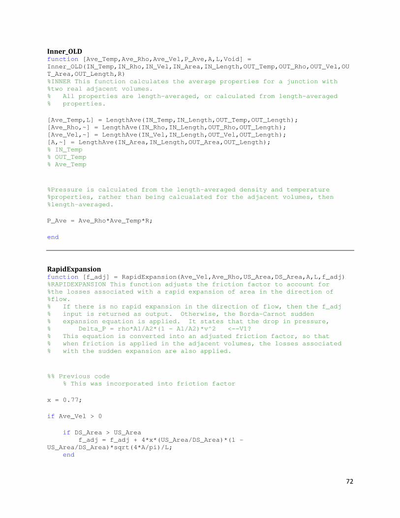
72

Inner_OLD function [Ave_Temp,Ave_Rho,Ave_Vel,P_Ave,A,L,Void] =

Inner_OLD(IN_Temp,IN_Rho,IN_Vel,IN_Area,IN_Length,OUT_Temp,OUT_Rho,OUT_Vel,OU

T_Area,OUT_Length,R) %INNER This function calculates the average properties for a junction with %two real adjacent volumes. % All properties are length-averaged, or calculated from length-averaged % properties.

[Ave_Temp,L] = LengthAve(IN_Temp,IN_Length,OUT_Temp,OUT_Length); [Ave_Rho,~] = LengthAve(IN_Rho,IN_Length,OUT_Rho,OUT_Length); [Ave_Vel,~] = LengthAve(IN_Vel,IN_Length,OUT_Vel,OUT_Length); [A,~] = LengthAve(IN_Area,IN_Length,OUT_Area,OUT_Length); % IN_Temp % OUT_Temp % Ave_Temp

%Pressure is calculated from the length-averaged density and temperature %properties, rather than being calcualated for the adjacent volumes, then %length-averaged.

P_Ave = Ave_Rho*Ave_Temp*R;

end

RapidExpansion function [f_adj] = RapidExpansion(Ave_Vel,Ave_Rho,US_Area,DS_Area,A,L,f_adj) %RAPIDEXPANSION This function adjusts the friction factor to account for %the losses associated with a rapid expansion of area in the direction of %flow. % If there is no rapid expansion in the direction of flow, then the f_adj % input is returned as output. Otherwise, the Borda-Carnot sudden % expansion equation is applied. It states that the drop in pressure, % Delta_P = rho*A1/A2*(1 - A1/A2)*v^2 <--V1? % This equation is converted into an adjusted friction factor, so that % when friction is applied in the adjacent volumes, the losses associated % with the sudden expansion are also applied.

%% Previous code % This was incorporated into friction factor

x = 0.77;

if Ave_Vel > 0

if DS_Area > US_Area f_adj = f_adj + 4*x*(US_Area/DS_Area)*(1 -

US_Area/DS_Area)*sqrt(4*A/pi)/L; end

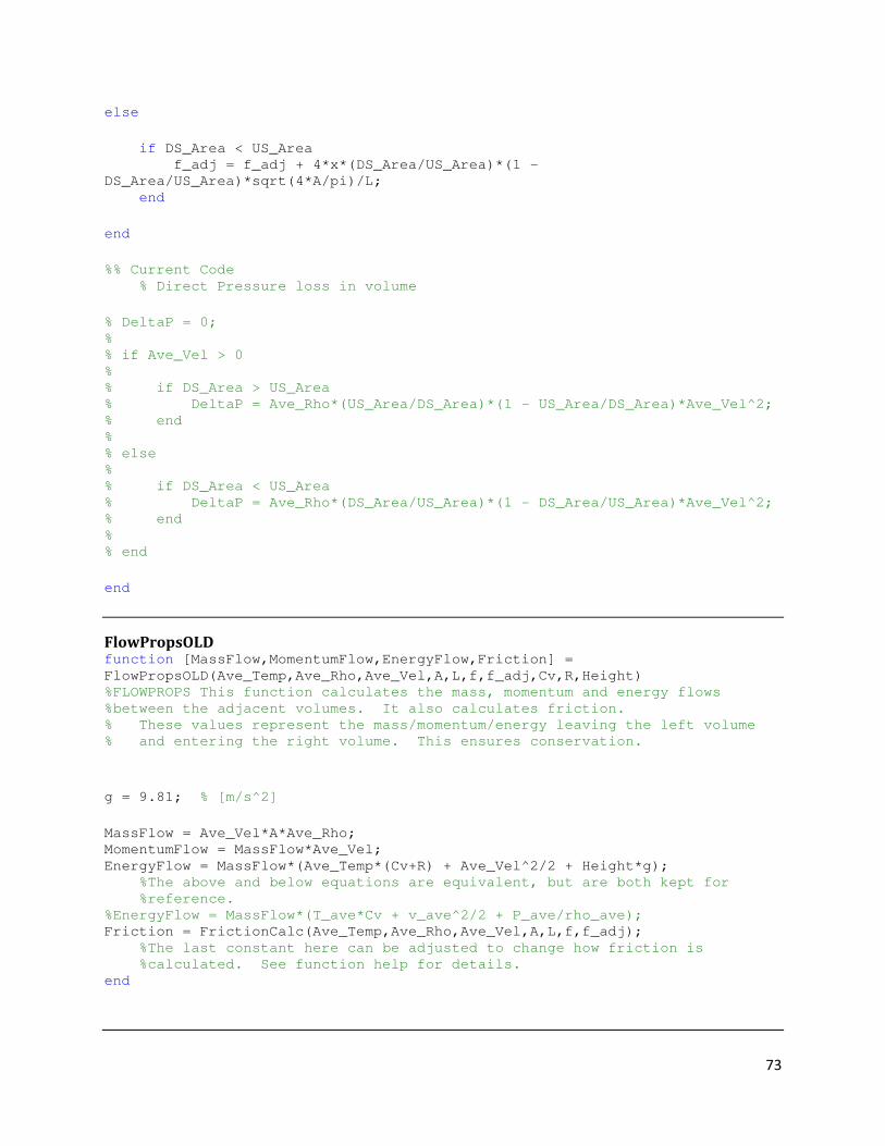
73

else

if DS_Area < US_Area f_adj = f_adj + 4*x*(DS_Area/US_Area)*(1 -

DS_Area/US_Area)*sqrt(4*A/pi)/L; end

end

%% Current Code % Direct Pressure loss in volume

% DeltaP = 0; % % if Ave_Vel > 0 % % if DS_Area > US_Area % DeltaP = Ave_Rho*(US_Area/DS_Area)*(1 - US_Area/DS_Area)*Ave_Vel^2; % end % % else % % if DS_Area < US_Area % DeltaP = Ave_Rho*(DS_Area/US_Area)*(1 - DS_Area/US_Area)*Ave_Vel^2; % end % % end

end

FlowPropsOLD function [MassFlow,MomentumFlow,EnergyFlow,Friction] =

FlowPropsOLD(Ave_Temp,Ave_Rho,Ave_Vel,A,L,f,f_adj,Cv,R,Height) %FLOWPROPS This function calculates the mass, momentum and energy flows %between the adjacent volumes. It also calculates friction. % These values represent the mass/momentum/energy leaving the left volume % and entering the right volume. This ensures conservation.

g = 9.81; % [m/s^2]

MassFlow = Ave_Vel*A*Ave_Rho; MomentumFlow = MassFlow*Ave_Vel; EnergyFlow = MassFlow*(Ave_Temp*(Cv+R) + Ave_Vel^2/2 + Height*g); %The above and below equations are equivalent, but are both kept for %reference. %EnergyFlow = MassFlow*(T_ave*Cv + v_ave^2/2 + P_ave/rho_ave); Friction = FrictionCalc(Ave_Temp,Ave_Rho,Ave_Vel,A,L,f,f_adj); %The last constant here can be adjusted to change how friction is %calculated. See function help for details. end

74

extrapolate function [y00] = extrapolate(y10,y21,y01,y02,y22,bound,percent) %EXTRAPOLATE This function extrapolates by space and time. It does not %allow the extrapolated value to exceed a bound by a certain percent. %The extrapolated bound must be within (percent*bound,bound/percent).

%% Extapolate:

%% Average two first-order extrapolations: (working, not for D,T,P BC)

% y00 = (2*y10 - y21 + 2*y01 - y02)/2; %Saving to back up.

%% 1st Order / 1st Order Attempt %While estimating y11

% %Estimate y11: % %This is the value in the adjacent volume for the previous time step. % % y11 = (y21 + y01)/2; % % % %Extrapolate using First-order in space and First-order in time: % % y00 = 2*y11 - y22;

%% Estimate y20 by time extrapolation, then find y00 by space extrapolation:

(working, not for D,T,P BC)

y20 = 2*y21 - y22; y00 = 2*y10 - y20;

%% Define upper and lower bounds, based on sign.

if bound >= 0 upper = bound/percent; lower = bound*percent; else upper = bound*percent; lower = bound/percent; end

%% Coerce to limits if extrapolated value is not within range.

if y00 < lower y00 = lower; elseif y00 > upper y00 = upper; end

end

75

LengthAve function [Ave_Prop,Total] = LengthAve(US_Prop,US_Length,DS_Prop,DS_Length) %LENGTHAVE This function averages aproperty based on the conditions in the %adjacent cells. % This function is weighted by length such that the resulting property is % more similar to the shorter cell (the cell with the closest center).

%Find the total Length:

Total = US_Length + DS_Length;

%Average by length weighting:

Ave_Prop = (DS_Length*US_Prop + US_Length*DS_Prop)/Total;

end

FrictionCalc function [Friction] = FrictionCalc(Ave_Temp,Ave_Rho,Ave_Vel,A,L,f,f_adj) %FRICTIONCALC This function calculates the frictional force exerted in the %junction, to be used by the adjacent volumes. This function has the %option to use different types of friction settings. % • If f = 0, Friction = 0, regardless of other parameters. Use this case % if you are using flow without friction. % • If f = 1, Friction is calculated from Reynolds number. Use this case % if you are using the smooth pipe calculations. % • For all other f, friction is calculated using a constant friction % factor (determined by f).

%If f = 0, do not bother with the rest of the calculations:, unless there %is an adjustment.

if f == 0 && f_adj == 0 Friction = 0; else

%Calculate needed properties:

Dh = sqrt(A*4/pi); % mu = 1.983e-5*sqrt(Ave_Temp/300); % mu = 0.0005 mu = exp(578.919/(Ave_Temp - 137.546) - 3.7188); Re = Ave_Rho*abs(Ave_Vel)*Dh/mu;

%Calculate f based on Re, if f = 1:

76

if f == 1 % if Re <= 1189.4 % f = 64/Re + f_adj; % elseif Re <= 49817.9 % f = 0.316*Re^(-1/4) + f_adj; % else % f = 0.184*Re^(-1/5) + f_adj; % end f = 0.0791*Re^(-1/4) + f_adj; else f = f + f_adj; end

%Calculate the force due to friction:

Tau = Ave_Vel^2*Ave_Rho*f/8; Friction = -sign(Ave_Vel)*L*Dh*pi*Tau/4; %NOTE: the 1/4 is because L refers to the total length of both %adjacent volumes. For this value to be used by volumes, it must %represent 1/2 of the length of a volume.

end

77

Volume Block Code

ICs function [Mass,Momentum,Energy,Volume,Height] =

ICs(Temperature,Density,Velocity,Area,Length,Angle,US_Height) SpHeatV = 724.96; % [J/kg-K] g = 9.81; % [m/s^2] Height = US_Height + Length*sin(Angle*pi/180); H = (Height + US_Height)/2; Volume = Area*Length; Mass = Volume*Density; Momentum = Mass*Velocity; Energy = Mass*(SpHeatV*Temperature + 0.5*Velocity^2 + g*H);

MomentumAdj function Force =

MomentumAdj(US_Press,US_Friction,US_Area,DS_Press,DS_Friction,DS_Area,V_Area,

V_Mass,Vel,L,Angle) %% MOMENTUMADJ %This function calculates all the forces applied to the momentum flow in %the volume cell.

g = 9.81; % [m/s^2] %% Ratio %This calculates the ratio of pressure in the x direction to total %pressure.

US_Dh = sqrt(4*US_Area/pi); DS_Dh = sqrt(4*DS_Area/pi); V_Dh = sqrt(4*V_Area/pi);

% US_R = (V_Dh - US_Dh)/sqrt((V_Dh - US_Dh)^2 + 4*L^2); % DS_R = (DS_Dh - V_Dh)/sqrt((DS_Dh - V_Dh)^2 + 4*L^2); % US_R = 0; % DS_R = 0;

x = 0;

%% Changing Area Calculations %This section calculates the area difference between the current volume and %adjacent volumes. If this volume's cross-sectional area is larger, an %adjustment to the pressure forces needs to be applied.

% if US_Area > 0 && DS_Area > 0 % % if US_Area < V_Area % US_Diff = V_Area - US_Area; % US_Diff = 0; % else % US_Diff = 0; % US_Area = V_Area; % end

78

% % if DS_Area < V_Area % DS_Diff = V_Area - DS_Area; % else % DS_Diff = 0; % DS_Area = V_Area; % end % % else % US_Diff = 0; % DS_Diff = 0; % end

%% Pressure Balance

% Pressure = US_Press*US_Area + x*US_Diff*V_Press - DS_Press*DS_Area -

x*DS_Diff*V_Press; % Pressure = US_Press*US_Area - DS_Press*DS_Area; Pressure = US_Area*US_Press + (DS_Area - US_Area)*(US_Press + DS_Press)/2 -

DS_Area*DS_Press;

%% Body Force

Fg = V_Mass*g*sin(pi*Angle/180);

%% Total Force

Force = Pressure + US_Friction + DS_Friction - Fg;

end

Volume function [Temperature,Density,Velocity,Pressure] =

Volume(Mass,Momentum,Energy,Volume,US_Height,Height) SpHeatV = 724.96; % [J/kg-K] R = 287.04; g = 9.81; % [m/s^2] H = (US_Height + Height)/2; Density = Mass/Volume; Velocity = Momentum/Mass; Temperature = (Energy/Mass - Velocity^2/2 - H*g)/SpHeatV; Pressure = Density*Temperature*R; % mu = 1.983e-5*(abs(Temperature)/300)^(1/2); % Dh = sqrt(4*Area/pi); % Re = Density*abs(Velocity)*Dh/mu; % if Re <= 1189.4 % f = 64/Re; % else % f = 0.316*Re^(-1/4);

79

% end % Tau = Velocity^2*Density*f/8; % Friction = sign(Velocity)*Length*Dh*pi*Tau; % US_P = US_VolumeProps.Density*US_VolumeProps.Temperature*R; % DS_P = DS_VolumeProps.Density*DS_VolumeProps.Temperature*R; % BodyForces = US_P*(Area*Length +

US_VolumeProps.Area*US_VolumeProps.Length)/(Length + US_VolumeProps.Length) -

DS_P*(Area*Length + DS_VolumeProps.Area*DS_VolumeProps.Length)/(Length +

DS_VolumeProps.Length) - Friction;

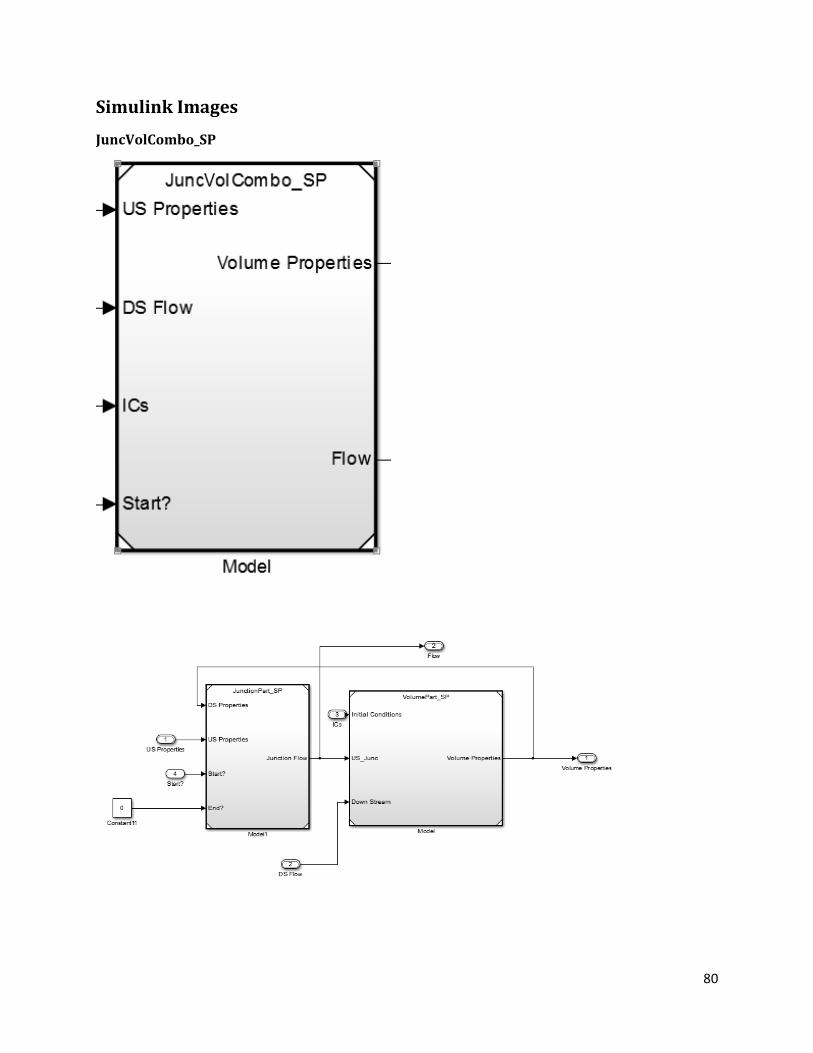
80

Simulink Images

JuncVolCombo_SP

81

JunctionPart_SP

82

VolumePart_SP

Subsystem (Integrator)

83

Appendix D: Two Phase Simulation Code Please note that functions used by both the single phase and two phase simulations are only shown in

“Appendix C: Single Phase Simulation Code.”

Junction Block Code

Junction_V function

[MassFlow,MomentumFlow,EnergyFlow,Ave_Temp,Ave_Vel,Ave_Rho,P_Ave,Void_Fractio

n] =

Junction_V(US_Temperature,US_Density,US_Velocity,US_Area,US_Length,US_Junc,DS

_Temperature,DS_Density,DS_Velocity,DS_Area,DS_Length,DS_Junc,Start,End_Press

ure,Last_Step,Last_2Step,US_Junc_OLD,DS_Junc_OLD,US_Vol,DS_Vol,Height) %JUNCTION This is the main function to calculate the flows and state %between two adjacent volumes (or on a boundary condition). % This function finds the average temperature, pressure and velocity % between two volumes (or on a boundary condition), then calculates the % mass, momentum and energy flows between the two volumes.

%% Constants

rho_water = 1000; % [kg/m^3] Cv = 724.96; % [J/kg-K] R = 287.04; % [J/kg-K] expercent = 0.8; f = 0; %This constant can be adjusted to change how friction is calculated. %See the help for the function "FrictionCalc" for details.

US_Void = US_Vol.Void_Fraction; DS_Void = US_Vol.Void_Fraction;

%% Junction Type Determination

if End_Pressure > 0 %% Right Boundary Condition

A = US_Area; Total_L = 2*US_Length;

if End_Pressure == 9999 [Ave_Temp,Ave_Rho,Ave_Vel,P_Ave,Void_Fraction] =

Outlet(US_Temperature,US_Density,US_Velocity,US_Void,DS_Temperature,DS_Densit

y,DS_Velocity,US_Junc,Last_Step,Last_2Step,US_Junc_OLD,expercent,R); else [Ave_Temp,Ave_Rho,Ave_Vel,P_Ave,Void_Fraction] =

Intlet(DS_Temperature,DS_Density,DS_Velocity,DS_Void,US_Temperature,US_Densit

y,US_Velocity,US_Junc,Last_Step,Last_2Step,US_Junc_OLD,expercent,R); end

elseif Start > 0 %% Left Boundary Condition

84

Total_L = 2*DS_Length; A = DS_Area;

if Start == 9999 [Ave_Temp,Ave_Rho,Ave_Vel,P_Ave,Void_Fraction] =

Intlet(US_Temperature,US_Density,US_Velocity,US_Void,DS_Temperature,DS_Densit

y,DS_Velocity,DS_Junc,Last_Step,Last_2Step,DS_Junc_OLD,expercent,R); else [Ave_Temp,Ave_Rho,Ave_Vel,P_Ave,Void_Fraction] =

Outlet(DS_Temperature,DS_Density,DS_Velocity,DS_Void,US_Temperature,US_Densit

y,US_Velocity,DS_Junc,Last_Step,Last_2Step,DS_Junc_OLD,expercent,R); end

else %% Interior Cells

[Ave_Temp,Ave_Rho,Ave_Vel,P_Ave,A,Total_L,Void_Fraction] =

Inner(US_Temperature,US_Density,US_Velocity,US_Area,US_Length,US_Void,DS_Temp

erature,DS_Density,DS_Velocity,DS_Area,DS_Length,DS_Void,R); end %% Two-phase mixing % Now that the average properties are determined, this section the % mixture ratio.

% [MassRatio,Mix_v] =

Mixing(US_Mass_R,US_Density,US_Length,US_Area,DS_Mass_R,DS_Density,DS_Length,

DS_Area,Ave_Rho,A,rho_water);

%% Other Losses % These losses are added to the friction factor.

A = Void_Fraction*A; f_adj = RapidExpansion(Ave_Vel,Ave_Rho,US_Area,DS_Area,A,Total_L,0);

% P_Ave = P_Ave + 2*P_loss;

%% Flow Calculations % To be used by adjacent volumes.

[MassFlow,MomentumFlow,EnergyFlow,~] =

FlowProps(Ave_Temp,Ave_Rho,Ave_Vel,P_Ave,A,Total_L,f,f_adj,Cv,Height,A);

end

Junction_L function [MassFlow,MomentumFlow,EnergyFlow,Friction,Ave_Temp,Ave_Vel] =

Junction_L(US_Temperature,US_Density,US_Velocity,US_Area,US_Length,US_Junc,DS

85

_Temperature,DS_Density,DS_Velocity,DS_Area,DS_Length,DS_Junc,Start,End_Press

ure,Last_Step,Last_2Step,US_Junc_OLD,DS_Junc_OLD,Ave_P,Void_Fraction,Height) %JUNCTION_L This is the main function to calculate the flows and state %between two adjacent volumes (or on a boundary condition). % This function finds the average temperature, pressure and velocity % between two volumes (or on a boundary condition), then calculates the % mass, momentum and energy flows between the two volumes.

%% Constants

C_water = 4180; % [J/kg-K] rho_water = 1000; % [kg/m^3] expercent = 0.8; f = 0.02; %0.032; %This constant can be adjusted to change how friction is calculated. %See the help for the function "FrictionCalc" for details. VF = 0; %Void Filler: Void fraction is already caclulated. Nearby void

fractions are not needed.

%% Junction Type Determination

if End_Pressure > 0 %% Right Boundary Condition

A = US_Area; Total_L = 2*US_Length;

if End_Pressure == 9999 [Ave_Temp,~,Ave_Vel,~,~] =

Outlet(US_Temperature,US_Density,US_Velocity,VF,DS_Temperature,DS_Density,DS_

Velocity,US_Junc,Last_Step,Last_2Step,US_Junc_OLD,expercent,0); else [Ave_Temp,~,Ave_Vel,~,~] =

Intlet(DS_Temperature,DS_Density,DS_Velocity,VF,US_Temperature,US_Density,US_

Velocity,US_Junc,Last_Step,Last_2Step,US_Junc_OLD,expercent,0); end

elseif Start > 0 %% Left Boundary Condition

Total_L = 2*DS_Length; A = DS_Area;

if Start == 9999 [Ave_Temp,~,Ave_Vel,~] =

Intlet(US_Temperature,US_Density,US_Velocity,VF,DS_Temperature,DS_Density,DS_

Velocity,DS_Junc,Last_Step,Last_2Step,DS_Junc_OLD,expercent,0); else [Ave_Temp,~,Ave_Vel,~] =

Outlet(DS_Temperature,DS_Density,DS_Velocity,VF,US_Temperature,US_Density,US_

Velocity,DS_Junc,Last_Step,Last_2Step,DS_Junc_OLD,expercent,0); end

86

else %% Interior Cells

[Ave_Temp,~,Ave_Vel,~,A,Total_L] =

Inner(US_Temperature,US_Density,US_Velocity,US_Area,US_Length,VF,DS_Temperatu

re,DS_Density,DS_Velocity,DS_Area,DS_Length,VF,0); end %% Two-phase mixing % Now that the average properties are determined, this section the % mixture ratio.

% [MassRatio,Mix_v] =

Mixing(US_Mass_R,US_Density,US_Length,US_Area,DS_Mass_R,DS_Density,DS_Length,

DS_Area,Ave_Rho,A,rho_water);

%% Other Losses % These losses are added to the friction factor.

Flow_A = (1 - Void_Fraction)*A; f_adj = RapidExpansion(Ave_Vel,rho_water,US_Area,DS_Area,A,Total_L,0);

%% Flow Calculations % To be used by adjacent volumes.

[MassFlow,MomentumFlow,EnergyFlow,Friction] =

FlowProps(Ave_Temp,rho_water,Ave_Vel,Ave_P,Flow_A,Total_L,f,f_adj,C_water,Hei

ght,A);

end

Outlet function [Ave_Temp,Ave_Rho,Ave_Vel,Ave_P,Void_Fraction] =

Outlet(IN_Temp,IN_Rho,IN_Vel,IN_Void,OUT_Temp,OUT_Rho,OUT_Vel,IN_Junc,Last_St

ep,Last_2Step,Adj_Junc,expercent,R) %OUTLET This function calculates the properties of a boundary condition that %is letting fluid out of the model. % This function calculates junction properties with a real volume inlet % and a constant outlet.

%Property extrapolation: % IN_Temp = IN_Temp % J_TempIN = IN_Junc.Temp % Last_Temp = Last_Step.Temp % Last_2Temp = Last_2Step.Temp % Adj_Temp = Adj_Junc.Temp

87

% expercent = expercent

Ave_Temp =

extrapolate(IN_Temp,IN_Junc.Temp,Last_Step.Temp,Last_2Step.Temp,Adj_Junc.Temp

,IN_Temp,expercent); Ave_Vel =

extrapolate(IN_Vel,IN_Junc.Vel,Last_Step.Vel,Last_2Step.Vel,Adj_Junc.Vel,IN_V

el,expercent);

if isfield(IN_Junc,'Rho') Ave_Rho =

extrapolate(IN_Rho,IN_Junc.Rho,Last_Step.Rho,Last_2Step.Rho,Adj_Junc.Rho,IN_R

ho,expercent); Void_Fraction =

extrapolate(IN_Void,IN_Junc.Void_Fraction,Last_Step.Void_Fraction,Last_2Step.

Void_Fraction,Adj_Junc.Void_Fraction,IN_Void,expercent); % disp('The average temperature is') % Ave_Temp = Ave_Temp %Calculate pressure based on type of boundary condition: else Ave_Rho = IN_Rho; Void_Fraction = 0; % disp('Liquid Temp:') % Ave_Temp = Ave_Temp end

if OUT_Vel == 0 Ave_P = OUT_Rho*OUT_Temp*R; else Ave_P = Ave_Rho*Ave_Temp*R; end

end

Inlet function [Ave_Temp,Ave_Rho,Ave_Vel,Ave_P,Void_Fraction] =

Intlet(IN_Temp,IN_Rho,IN_Vel,IN_Void,OUT_Temp,OUT_Rho,OUT_Vel,OUT_Junc,Last_S

tep,Last_2Step,Adj_Junc,expercent,R) %INLET This function performs calculations for the boundary condition that %fluid is flowing into. % This calculates junction properties from upstream constants and % properties from a real downstream cell.

%Pass Constants:

Ave_Temp = IN_Temp; Ave_Rho = IN_Rho; Ave_P = IN_Temp*IN_Rho*R; Void_Fraction = IN_Void;

88

%Calculate Velocity based on BC method:

if IN_Vel == 0 Ave_Vel =

extrapolate(OUT_Vel,OUT_Junc.Vel,Last_Step.Vel,Last_2Step.Vel,Adj_Junc.Vel,OU

T_Vel,expercent); else Ave_Vel = IN_Vel; Ave_P = 0; end

end

Inner function [Ave_Temp,Ave_Rho,Ave_Vel,P_Ave,A,L,Void] =

Inner(IN_Temp,IN_Rho,IN_Vel,IN_Area,IN_Length,IN_Void,OUT_Temp,OUT_Rho,OUT_Ve

l,OUT_Area,OUT_Length,OUT_Void,R) %INNER This function calculates the average properties for a junction with %two real adjacent volumes. % All properties are length-averaged, or calculated from length-averaged % properties.

[Ave_Temp,L] = LengthAve(IN_Temp,IN_Length,OUT_Temp,OUT_Length); [Ave_Rho,~] = LengthAve(IN_Rho,IN_Length,OUT_Rho,OUT_Length); [Ave_Vel,~] = LengthAve(IN_Vel,IN_Length,OUT_Vel,OUT_Length); [A,~] = LengthAve(IN_Area,IN_Length,OUT_Area,OUT_Length); [Void,~] = LengthAve(IN_Void,IN_Length,OUT_Void,OUT_Length); % IN_Temp % OUT_Temp % Ave_Temp

%Pressure is calculated from the length-averaged density and temperature %properties, rather than being calcualated for the adjacent volumes, then %length-averaged.

P_Ave = Ave_Rho*Ave_Temp*R;

end

FlowProps function [MassFlow,MomentumFlow,EnergyFlow,Friction] =

FlowProps(Ave_Temp,Ave_Rho,Ave_Vel,Ave_P,A,L,f,f_adj,C,Height,Friction_A) %FLOWPROPS This function calculates the mass, momentum and energy flows %between the adjacent volumes. It also calculates friction. % These values represent the mass/momentum/energy leaving the left volume % and entering the right volume. This ensures conservation.

g = 9.81; % [m/s^2]

MassFlow = Ave_Vel*A*Ave_Rho;

89

MomentumFlow = MassFlow*Ave_Vel; % EnergyFlow = MassFlow*(Ave_Temp*(Cv+R) + Ave_Vel^2/2); %The above and below equations are equivalent, but are both kept for %reference. EnergyFlow = MassFlow*(Ave_Temp*C + Ave_Vel^2/2 + Ave_P/Ave_Rho + Height*g); Friction = FrictionCalc(Ave_Temp,Ave_Rho,Ave_Vel,Friction_A,L,f,f_adj); %The last constant here can be adjusted to change how friction is %calculated. See function help for details. end

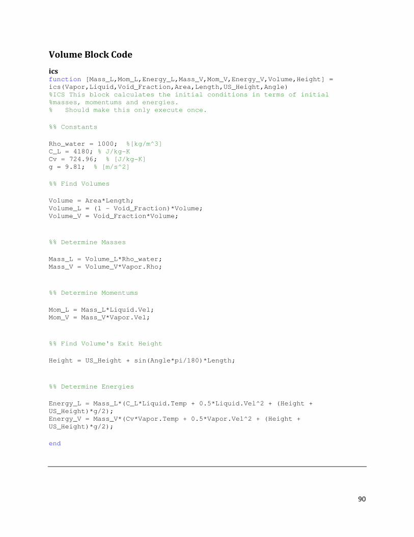
90

Volume Block Code

ics function [Mass_L,Mom_L,Energy_L,Mass_V,Mom_V,Energy_V,Volume,Height] =

ics(Vapor,Liquid,Void_Fraction,Area,Length,US_Height,Angle) %ICS This block calculates the initial conditions in terms of initial %masses, momentums and energies. % Should make this only execute once.

%% Constants

Rho_water = 1000; %[kg/m^3] C_L = 4180; % J/kg-K Cv = 724.96; % [J/kg-K] g = 9.81; % [m/s^2]

%% Find Volumes

Volume = Area*Length; Volume_L = (1 - Void_Fraction)*Volume; Volume_V = Void_Fraction*Volume;

%% Determine Masses

Mass_L = Volume_L*Rho_water; Mass_V = Volume_V*Vapor.Rho;

%% Determine Momentums

Mom_L = Mass_L*Liquid.Vel; Mom_V = Mass_V*Vapor.Vel;

%% Find Volume's Exit Height

Height = US_Height + sin(Angle*pi/180)*Length;

%% Determine Energies

Energy_L = Mass_L*(C_L*Liquid.Temp + 0.5*Liquid.Vel^2 + (Height +

US_Height)*g/2); Energy_V = Mass_V*(Cv*Vapor.Temp + 0.5*Vapor.Vel^2 + (Height +

US_Height)*g/2);

end

91

flowadjustments function

[Mass_L_IN,Mass_L_OUT,Momentum_L_IN,Momentum_L_OUT,Energy_L_IN,Energy_L_OUT,M

ass_V_IN,Mass_V_OUT,Momentum_V_IN,Momentum_V_OUT,Energy_V_IN,Energy_V_OUT] =

flowadjustments(US_Junction,DS_Junction,VolumeData,Area,Length,Angle) %FLOWADJUSTMENTS This function takes the upstream and downstream flows and %determines the change in mass, momentum and energy for the volume. % Inputs are busses that are split once they enter this function.

%% Constants

rho_water = 1000; R = 287.04;

Vol_Press = VolumeData.Vapor.Press; Void_Fraction = VolumeData.Void_Fraction; Vapor_Vel = VolumeData.Vapor.Vel; Vapor_Temp = VolumeData.Vapor.Temp; Vapor_Rho = VolumeData.Vapor.Rho; Liquid_Vel = VolumeData.Liquid.Vel; Liquid_Temp = VolumeData.Liquid.Temp;

%% Mass Balance % This section will contain the logic for mass transfer between liquid % and vapor in the future.

Mass_L_IN = US_Junction.MassFlow_L; Mass_L_OUT = DS_Junction.MassFlow_L; Mass_V_IN = US_Junction.MassFlow_V; Mass_V_OUT = DS_Junction.MassFlow_V;

%% Changing Area Calculations %This section calculates the area difference between the current volume and %adjacent volumes. If this volume's cross-sectional area is larger, an %adjustment to the pressure forces needs to be applied.

US_Area = US_Junction.US_Area; DS_Area = DS_Junction.DS_Area; US_Press = US_Junction.Pressure; DS_Press = DS_Junction.Pressure; US_VF = US_Junction.Void_Fraction; DS_VF = DS_Junction.Void_Fraction; Dh = 2*sqrt(Area/pi);

% if US_Area > 0 && DS_Area > 0 % % if US_Area < Area % US_Diff = Area - US_Area; % else % US_Diff = 0; % US_Area = Area;

92

% end % % if DS_Area < Area % DS_Diff = Area - DS_Area; % else % DS_Diff = 0; % DS_Area = Area; % end % % else % US_Diff = 0; % DS_Diff = 0; % end

%% Pressure Calculations

% Pressure = US_Junction.Pressure*US_Area + US_Diff*Vol_Press -

DS_Junction.Pressure*DS_Area - DS_Diff*Vol_Press; US_V_A = US_VF*US_Area; DS_V_A = DS_VF*DS_Area; US_L_A = (1 - US_VF)*US_Area; DS_L_A = (1 - DS_VF)*DS_Area; Pressure_Vapor = US_V_A*US_Press + (DS_V_A - US_V_A)*(US_Press + DS_Press)/2

- DS_V_A*DS_Press; Pressure_Liquid = US_L_A*US_Press + (DS_L_A - US_L_A)*(US_Press + DS_Press)/2

- DS_L_A*DS_Press;

%% Interphase Drag

f_int = 1; deltaV = Vapor_Vel - Liquid_Vel; drag = f_int*Void_Fraction*(1 -

Void_Fraction)*rho_water*sign(deltaV)*deltaV^2/Dh; dragforce = drag*Area*Length; % dragforce = 10*deltaV; % Dh_int = sqrt(Void_Fraction*Area*4/pi); % Tau_int = deltaV^2*Vapor_Rho*f_int/8; % dragforce = sign(deltaV)*Length*Dh_int*pi*Tau_int;

%% Interphase Heat Transfer

h = 50000; % [W/m^3-K] Delta_T = Vapor_Temp - Liquid_Temp; Q_dot = h*Delta_T*Void_Fraction*(1 - Void_Fraction)*Area*Length;

%% Energy Balance

% Work (rate) Done by friction: % W_out,V = V_vap * F_d % W_in,L = V_liq * F_d % W_lost = (V_vap - V_liq) * F_d % Assuming energy dissapates into both phases equally, half of "lost"

93

% energy stays in the vapor phase.

% Net energy transfered from Vapor to liquid: W_net = dragforce*(Liquid_Vel + Vapor_Vel)/2;

% Work (rate) Done by expansion (changing volume of a fluid) %W = P*dVol/dt %dVol_L/dt = m_dot_L/rho_L

Ave_VF = (US_VF + DS_VF)/2; W_exp = Vol_Press*(Mass_L_IN - Mass_L_OUT)/rho_water +

0.5*R*Vapor_Temp*(Vapor_Rho*(Mass_L_IN - Mass_L_OUT)/rho_water + (Mass_L_IN -

Mass_L_OUT))*(Area*Length)*(1 - 2*Ave_VF);

% This work term matches the kinetic energy transfer due to drag force. % If energy was kept the same, then internal energy would increase/decrease % based on the momentum change. By transfering energy from one phase or % another, only velocity is affected by friction.

Energy_L_IN = US_Junction.EnergyFlow_L + Q_dot + W_net + W_exp; Energy_L_OUT = DS_Junction.EnergyFlow_L; Energy_V_IN = US_Junction.EnergyFlow_V - Q_dot - W_net - W_exp; Energy_V_OUT = DS_Junction.EnergyFlow_V;

%% Body Forces

Weight_L = rho_water*Area*Length*(1 - Void_Fraction)*sin(Angle*pi/180); Weight_V = Vapor_Rho*Area*Length*Void_Fraction*sin(Angle*pi/180);

%% Momentum Balance

% massfrac = Void_Fraction*Vapor_Rho/((1-Void_Fraction)*rho_water);

Momentum_L_IN = US_Junction.MomentumFlow_L + Pressure_Liquid +

US_Junction.Friction + DS_Junction.Friction + dragforce - Weight_L; Momentum_L_OUT = DS_Junction.MomentumFlow_L; Momentum_V_IN = US_Junction.MomentumFlow_V + Pressure_Vapor - dragforce -

Weight_V; Momentum_V_OUT = DS_Junction.MomentumFlow_V;

end

Volume function

[Vapor_Temp,Vapor_Vel,Vapor_Rho,Vapor_Press,Liquid_Temp,Liquid_Vel,Void_Fract

ion] = Volume(Mass_L,Mom_L,Energy_L,Mass_V,Mom_V,Energy_V,Vol,Height) %VOLUME This function uses the mass, momentum and energy present within a

94

%volume to calculate the properties of the liquid and vapor present. % The output is 2 busses. Vapor contains the vapor properties of the % volume (Density, Temperature, Pressure, Velocity) and Liquid contains % the liquid properties (Temperature and Velocity).

%% Constants

Rho_L = 1000; % [kg/m^3] C_L = 4180; % [J/kg-K] Cv = 724.96; % [J/kg-K] R = 287.04; % [J/kg-K]

%% Find Void Fraction

if Mass_L > 0 Void_Fraction = 1 - Mass_L/(Rho_L*Vol); else Void_Fraction = 1; end

%% Determine Liquid Properties

[Liquid_Temp,Liquid_Vel] = tempvel(Mass_L,Mom_L,Energy_L,C_L,Height);

%% Determine Vapor Properties

Vapor_Rho = Mass_V/(Void_Fraction*Vol); [Vapor_Temp,Vapor_Vel] = tempvel(Mass_V,Mom_V,Energy_V,Cv,Height); Vapor_Press = Vapor_Rho*Vapor_Temp*R;

end

tempvel function [Temperature,Velocity] = tempvel(Mass,Momentum,Energy,C,Height) %TEMPVEL This function calculates temperature and velocity. % Formulations for liquid and vapor are the same.

g = 9.81; % [m/s^2]

Velocity = Momentum/Mass; Temperature = (Energy/Mass - Velocity^2/2 - Height*g)/C;

end

95

Simulink Images

JuncVolCombo

96

JunctionPart

97

VolumePart