Embed Size (px)
Citation preview
Master's Degree Thesis ISRN: BTH-AMT-EX--2012/D-17--SE
Supervisors: Niklas Philipson, Scania Peter Daelander, Scania Ansel Berghuvud, BTH
Department of Mechanical Engineering Blekinge Institute of Technology
Karlskrona, Sweden
2012
Masoud Vahedi
Development and Validation of Dynamic Belt Transmission Model
in Dymola

Development and Validation of Dynamic Belt Transmission
Model in Dymola
Masoud Vahedi
Blekinge Institute of Technology, Karlskrona, Sweden
Scania Company, Södertälje, Sweden (August 2012)
Thesis submitted for completion of Master of Science in Mechanical Engineering with emphasis on Structural Mechanics at the Department of Mechanical Engineering, Blekinge Institute of Technology, Karlskrona, Sweden.
Abstract: For making a generic model of planar belt drive systems in Dymola, the project is divided in two steps; First, the Planar Multibody Library (PML), which is built of general components for use in two-dimensional applications such as mass, revolute joint and beam element. Second, modelling of the Scania Belt Drive Library (SBDL) by using the components in the first step and making some new components specially designed for belt drive simulations. Results of the Scania Belt Drive Library are validated against the experimental data and AVL/Timing Drive.
Advantages such as the possibility of changing or updating the components equations, start up simulation, being less error prone due to user inputs, and even simulation performance are the major reasons for which the Scania Belt Drive Library has been created.
Modelling of a component in Dymola demands deriving the necessary equations of motion for that special component.
Keywords: Belt Drive System, Non-Toothed Belt, Pulley, Theoretical Model, Contact Model, Dymola, Modelica.

2
Acknowledgements
This thesis work was carried out at Scania AB, NMBD, in cooperation with the Department of Mechanical Engineering, Blekinge Institute of Technology (BTH), under the supervision of Dr. Ansel Berghuvud (BTH), Niklas Philipson (Scania) and Peter Daelander (Scania).
I would like to record my sincere appreciation to Niklas Philipson, Senior Engineer, for his guidance and professional engagement throughout the work and whose knowledge and skills helped me throughout the project. I wish to thank Dr. Ansel Berghuvud for discussions and support.
Furthermore, I would like to thank Scania staff who provided a pleasant and friendly working environment.
Lastly, I would like to express my deep gratitude to all my family and friends that like always supported me in all conditions.
Sweden, August 2012
Masoud Vahedi
3
Contents
Notation 5
1 Introduction 7 1.1 Dymola Software and Modelica Language 7
2 Overview 9
3 Planar Multibody Library 11 3.1 Frames 11 3.2 Mass 12 3.3 Fixed 12 3.4 Fixed Translation 13 3.5 Fixed Rotation 14 3.6 Revolute Joint 14 3.7 Prismatic Joint 15 3.8 Rotational Friction 16 3.9 Massless-beam 17
3.9.1 Massless Beam Equations 19 3.10 Sensors 21 3.11 Force and Torque Components 21
4 Scania Belt Drive Library 23 4.1 Belt 23 4.2 Pulley 24
4.2.1 Contact Model 25 4.3 Tensioner 29 4.4 Engine 30 4.5 Water Pump Torque Component 30 4.6 Initial Condition Calculations 31 4.7 Complete Belt Drive System Model 31
5 Validation 33 5.1 Planar Multibody Library 33 5.2 Scania Belt Drive Library 34
6 Performance Investigations 39 6.1 Selection of Integration Algorithm 39 6.2 Elimination of Time and State Events in the Model 40 6.3 Other Techniques 41
7 Polygon Effect 42
4
8 Scania Belt Drive Library vs. AVL/Timing Drive 44
9 Possible Complementary Works in Future 45
10 Conclusion 46
11 References 47
12 Appendix 48 12.1 Initialization 48
12.1.1 Link-points position vectors 49 12.1.2 Belt wrap angle for each pulley 50 12.1.3 Initial position vectors of the belt elements 51 12.1.4 Initial velocity vectors of the belt elements 54 12.1.5 Initial angle of the belt elements 55 12.1.6 Initial angular velocity of the pulleys 56 12.1.7 Initial angular velocity of the belt elements 56 12.1.8 Loaded and unloaded belt length 56 12.1.9 Tensioner torque 57
12.2 SBDL User Manual 58 12.2.1 Initialization Part 58 12.2.2 Assembling of the Layout 59 12.2.3 Simulation Setting 60
12.3 Software Environment 61
5
Notation
a Acceleration vector
φ Angle
α Angular acceleration
ω Angular velocity
A Area
× Cross product
c Damping coefficient
F Force
휇 Friction coefficient
g Gravitational acceleration
Length of a vector
L Loaded belt length
M Mass I Mass moment of inertia
Normalized version of vector
r Position vector R Radius
Relative vector from b to a
. Scalar product (dot product)
푠 Slippage
k Spring coefficient
휏 Torque
T Transformation matrix
L Unloaded belt length
v Velocity vector
6
E Young’s modulus Abbreviations CW Clockwise
CCW Counter Clockwise MSL Modelica Standard Library
PML Planar Multibody Library SBDL Scania Belt Drive Library
7
1 Introduction
The aim of the thesis is to build a generic belt drive system model-library in Dymola (Dynamic Modelling Laboratory), suited for dynamic analysis of belt drive transmissions. Belt drive system simulation is important from different points of view; knowing about the angular displacement of the tensioner, longitudinal force in the belt, loads on the pulley’s bearings and in general having a good understanding of the dynamic motion of the belt drive system are all crucial for designing better pulley and belt layouts.
AVL/Timing Drive is one software solution which is typically used for belt drive simulations within Scania. Because of certain weaknesses such as being error-prone in inputting of data, complexity in modelling, size limitations on results files, as well as high cost, other simulation environments are considered. Dymola is one of the well-known simulation environments in studies of dynamic systems. So it was the time to evaluate its potential for belt drive system analysis [1].
Measurement data and simulation results of engine belt drive systems in AVL/Timing Drive were present for comparison with the results of Scania Belt Drive Library. For modelling of a component in Dymola, the user should script the equations of motion of that special component in Modelica language - the programming language of Dymola software. A brief explanation of Dymola and Modelica language is presented in the next section. 1.1 Dymola Software and Modelica Language
Dymola is one of the new modelling methodologies and is based on object-oriented programming. Supporting of hierarchical model composition, libraries of truly reusable components, a-casual connections and available model libraries in many engineering domains (Multi-physics) are some of the important characteristics of this software [2].
8
Furthermore, being open for user-defined model components, good handling of differential algebraic equations, the possibility to write equations of motion in both declarative and algorithmic manners and the ability to reuse a component for different configurations are the major advantages for which this software was chosen for use in this thesis [2,3]. Other important highlights of Dymola are:
Good interface to other programs 3D animation ability. Handling of large, complex multi-engineering models. Faster simulation – symbolic pre-processing. Real-time simulation.
Compared to other similar software such as Matlab/Simulink, Dymola can use a-casual connections; so the direction of connection does not matter in the connection lines. In contrast with algorithmic programming, Dymola is also able to support declarative equations. Therefore, components equations can be written as they are, instead of deriving the right hand side of equations.
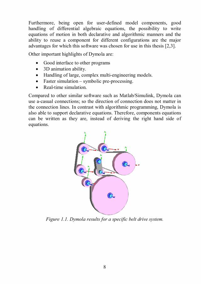
Figure 1.1. Dymola results for a specific belt drive system.
9
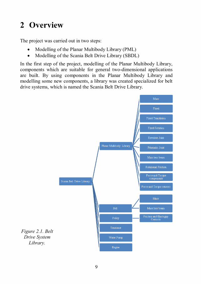
2 Overview
The project was carried out in two steps:
Modelling of the Planar Multibody Library (PML) Modelling of the Scania Belt Drive Library (SBDL)
In the first step of the project, modelling of the Planar Multibody Library, components which are suitable for general two-dimensional applications are built. By using components in the Planar Multibody Library and modelling some new components, a library was created specialized for belt drive systems, which is named the Scania Belt Drive Library.
Figure 2.1. Belt Drive System
Library.

10
In Figure (2.1) the various components modelled in each step are shown. In the following sections, each component and its modelling equations will be described according to the order of the diagram. Before starting to express the component’s equations, it is necessary to explain some of the functions which are generally used in the components equations.
The transformation matrix is used for transforming vectors from a local reference frame to a global coordinate system or vice versa. In figure(2.2), 퐹 is created by rotating vector 퐹 an angle 휃 in the positive direction (as defined by right hand rule). 퐹 can be calculated from equation (2.1).
Figure 2.2. 퐹 is the rotated version of 퐹 for angle 휃 in the positive
direction.
퐹 = 퐹 푇(휃) , 푇(휃) = cos (휃) −sin (휃)sin (휃) cos (휃)
(2.1)
In the above equation 푇(휃) is the transformation matrix, which rotates 퐹 for angle 휃 in the positive direction.
It should be noted, that since the library is designed for planar applications, the torque vector is always perpendicular to the plane; so there is no difference between the torque values in the local and global frames. For this reason, the torque vector is considered as a scalar variable in the library’s components. Another consideration which should be mentioned for planar condition is if 푎 = (푎 , 푎 ) and 푏 = (푏 , 푏 ) then 푎 × 푏 is defined as: 푎 × 푏 = 푎 푏 −푎 푏 . This notation is used quite often in the torque equations of components.
11
3 Planar Multibody Library
3.1 Frames
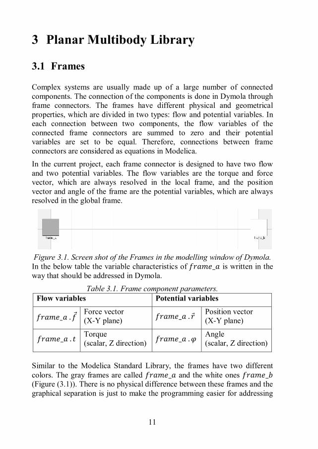
Complex systems are usually made up of a large number of connected components. The connection of the components is done in Dymola through frame connectors. The frames have different physical and geometrical properties, which are divided in two types: flow and potential variables. In each connection between two components, the flow variables of the connected frame connectors are summed to zero and their potential variables are set to be equal. Therefore, connections between frame connectors are considered as equations in Modelica. In the current project, each frame connector is designed to have two flow and two potential variables. The flow variables are the torque and force vector, which are always resolved in the local frame, and the position vector and angle of the frame are the potential variables, which are always resolved in the global frame.
Figure 3.1. Screen shot of the Frames in the modelling window of Dymola. In the below table the variable characteristics of 푓푟푎푚푒_푎 is written in the way that should be addressed in Dymola.
Table 3.1. Frame component parameters. Flow variables Potential variables
푓푟푎푚푒_푎 . 푓 Force vector (X-Y plane) 푓푟푎푚푒_푎 . 푟 Position vector
(X-Y plane)
푓푟푎푚푒_푎 . 푡 Torque (scalar, Z direction) 푓푟푎푚푒_푎 . 휑 Angle
(scalar, Z direction)
Similar to the Modelica Standard Library, the frames have two different colors. The gray frames are called 푓푟푎푚푒_푎 and the white ones 푓푟푎푚푒_푏 (Figure (3.1)). There is no physical difference between these frames and the graphical separation is just to make the programming easier for addressing
12
the frames, especially in the case where there is more than one frame in a component. 3.2 Mass
There is just one frame connector in the Mass component, where its equations of motion can be described as below:
푟 = 푓푟푎푚푒_푎 . 푟, 푣 = (푟), 푎 = (푣)
휑 = 푓푟푎푚푒_푎 . 푝ℎ푖, 휔 = (휑), 훼 = (휔)
(3.1) (3.2)
The force vector is resolved in the local frame. Therefore, the global acceleration vector should be transformed from the global frame to the local coordinate system in 푓푟푎푚푒_푎. The force and torque equations of the mass component are:
푓 = 푚 푎 푇(−휑)
휏 = 퐼훼
(3.3) (3.4)
Where m is mass, I is the moment of inertia and 푇(−휑) is the transformation matrix from the global coordinate system to the local coordinate system in 푓푟푎푚푒_푎. The gravity effect of the mass component is not included in the above equations of motion. 3.3 Fixed
The Fixed component has one connector (푓푟푎푚푒_푏) for which the position vector and angle are the only parameters of this component. The user is able to define these parameters (푟 and 휑) in the parameter window according to the desired system configuration.
푟 = 푓푟푎푚푒_푏 . 푟, 휑 = 푓푟푎푚푒_푏 . 푝ℎ푖
(3.5)
13
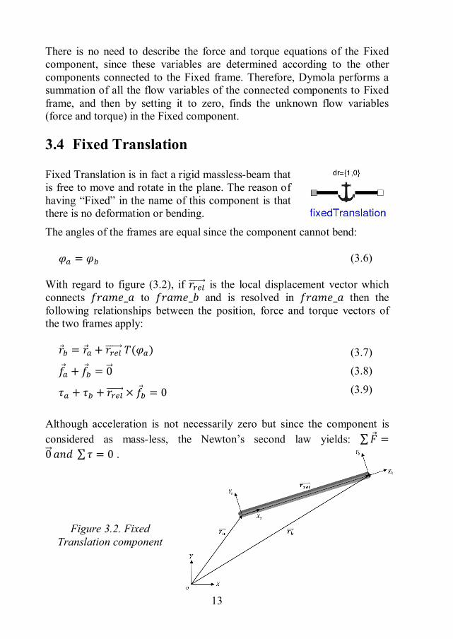
There is no need to describe the force and torque equations of the Fixed component, since these variables are determined according to the other components connected to the Fixed frame. Therefore, Dymola performs a summation of all the flow variables of the connected components to Fixed frame, and then by setting it to zero, finds the unknown flow variables (force and torque) in the Fixed component. 3.4 Fixed Translation
Fixed Translation is in fact a rigid massless-beam that is free to move and rotate in the plane. The reason of having “Fixed” in the name of this component is that there is no deformation or bending.
The angles of the frames are equal since the component cannot bend: 휑 = 휑
(3.6)
With regard to figure (3.2), if 푟 is the local displacement vector which connects 푓푟푎푚푒_푎 to 푓푟푎푚푒_푏 and is resolved in 푓푟푎푚푒_푎 then the following relationships between the position, force and torque vectors of the two frames apply:
푟 = 푟 + 푟 푇(휑 )
푓 + 푓 = 0
휏 + 휏 + 푟 × 푓 = 0
(3.7) (3.8)
(3.9)
Although acceleration is not necessarily zero but since the component is considered as mass-less, the Newton’s second law yields: ∑ 퐹 =0 푎푛푑 ∑ 휏 = 0 .
Figure 3.2. Fixed
Translation component
14
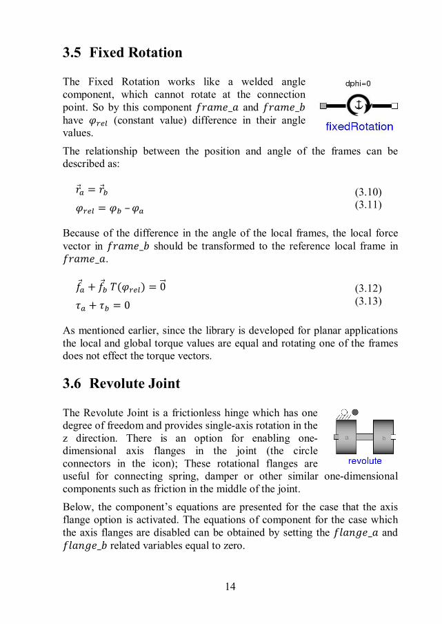
3.5 Fixed Rotation
The Fixed Rotation works like a welded angle component, which cannot rotate at the connection point. So by this component 푓푟푎푚푒_푎 and 푓푟푎푚푒_푏 have 휑 (constant value) difference in their angle values.
The relationship between the position and angle of the frames can be described as:
푟 = 푟
휑 = 휑 – 휑
(3.10) (3.11)
Because of the difference in the angle of the local frames, the local force vector in 푓푟푎푚푒_푏 should be transformed to the reference local frame in 푓푟푎푚푒_푎.
푓 + 푓 푇(휑 ) = 0
휏 + 휏 = 0
(3.12) (3.13)
As mentioned earlier, since the library is developed for planar applications the local and global torque values are equal and rotating one of the frames does not effect the torque vectors. 3.6 Revolute Joint
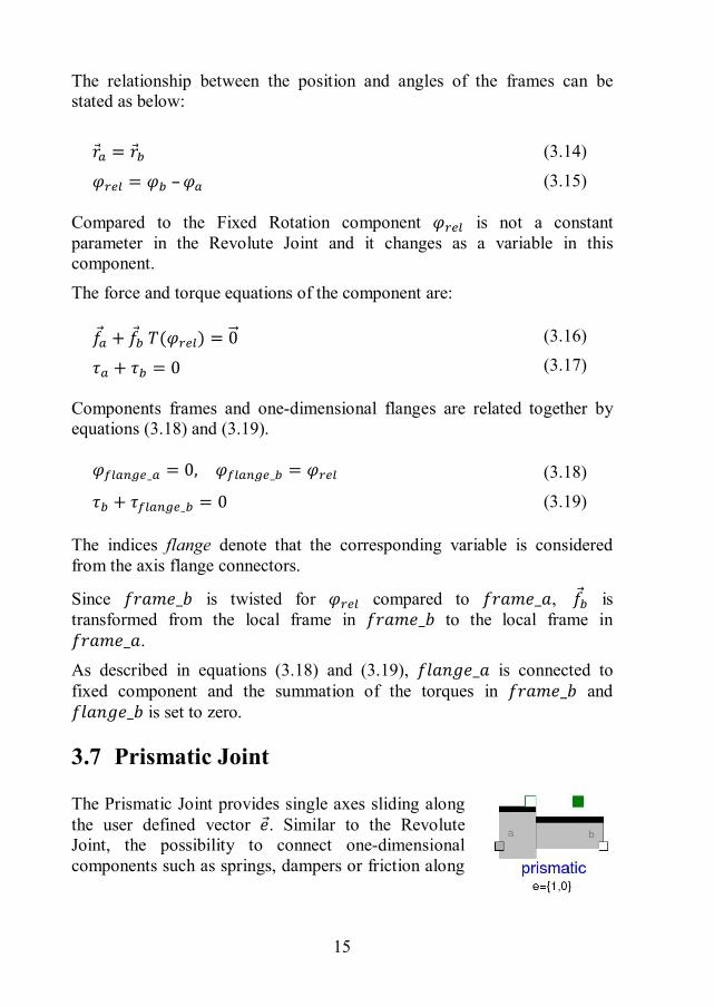
The Revolute Joint is a frictionless hinge which has one degree of freedom and provides single-axis rotation in the z direction. There is an option for enabling one-dimensional axis flanges in the joint (the circle connectors in the icon); These rotational flanges are useful for connecting spring, damper or other similar one-dimensional components such as friction in the middle of the joint. Below, the component’s equations are presented for the case that the axis flange option is activated. The equations of component for the case which the axis flanges are disabled can be obtained by setting the 푓푙푎푛푔푒_푎 and 푓푙푎푛푔푒_푏 related variables equal to zero.
15
The relationship between the position and angles of the frames can be stated as below:
푟 = 푟
휑 = 휑 – 휑
(3.14)
(3.15)
Compared to the Fixed Rotation component 휑 is not a constant parameter in the Revolute Joint and it changes as a variable in this component.
The force and torque equations of the component are: 푓 + 푓 푇(휑 ) = 0
휏 + 휏 = 0
(3.16) (3.17)
Components frames and one-dimensional flanges are related together by equations (3.18) and (3.19).
휑 _ = 0, 휑 _ = 휑
휏 + 휏 _ = 0
(3.18)
(3.19)
The indices flange denote that the corresponding variable is considered from the axis flange connectors.
Since 푓푟푎푚푒_푏 is twisted for 휑 compared to 푓푟푎푚푒_푎, 푓 is transformed from the local frame in 푓푟푎푚푒_푏 to the local frame in 푓푟푎푚푒_푎.
As described in equations (3.18) and (3.19), 푓푙푎푛푔푒_푎 is connected to fixed component and the summation of the torques in 푓푟푎푚푒_푏 and 푓푙푎푛푔푒_푏 is set to zero. 3.7 Prismatic Joint
The Prismatic Joint provides single axes sliding along the user defined vector 푒. Similar to the Revolute Joint, the possibility to connect one-dimensional components such as springs, dampers or friction along
16
the sliding direction of the joint is prepared by enabling the axis flange option.
In following, the general equations of this component are presented. For the case in which the axis flange option is turned off in the joint, the equation terms that are related to the flanges will disappear in the equations.
푟 = 푟 + 푟 푛 푇(휑 )
휑 = 휑
(3.20)
(3.21)
Where 푟 is the relative distance between 푓푟푎푚푒_푎 and 푓푟푎푚푒_푏 and 푛 is the normalized vector of the vector 푒, which shows the sliding direction in the local frame.
The force and torque equations of the Prismatic Joint are stated below: 푓 + 푓 = 0
휏 + 휏 + 푟 푛 × 푓 = 0
(3.22)
(3.23)
Components frames and one-dimensional flanges are related together by equations (3.24) and (3.25).
푟 _ = 0, 푟 _ = 푟
푓 . 푛 + 푓 _ = 0
(3.24)
(3.25)
For having a degree of freedom along the sliding direction, the force summation is equalled to zero in equation (3.25).
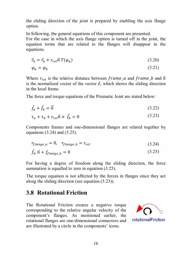
The torque equation is not affected by the forces in flanges since they act along the sliding direction (see equation (3.23)). 3.8 Rotational Friction
The Rotational Friction creates a negative torque corresponding to the relative angular velocity of the component’s flanges. As mentioned earlier, the rotational flanges are one-dimensional connectors and are illustrated by a circle in the components’ icons.
17
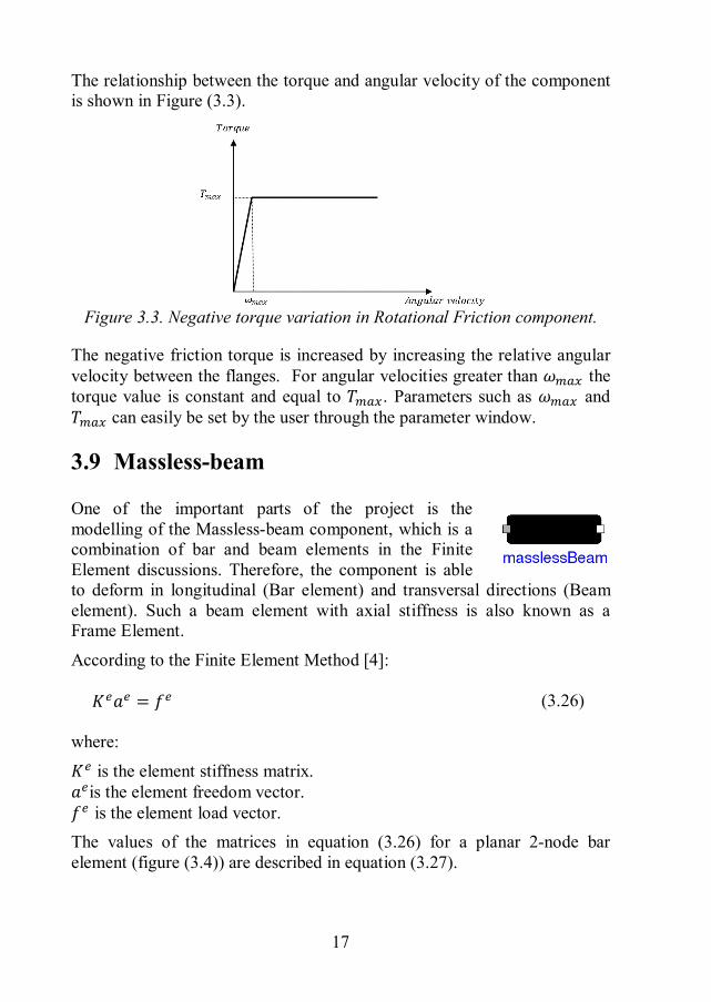
The relationship between the torque and angular velocity of the component is shown in Figure (3.3).
Figure 3.3. Negative torque variation in Rotational Friction component.
The negative friction torque is increased by increasing the relative angular velocity between the flanges. For angular velocities greater than 휔 the torque value is constant and equal to 푇 . Parameters such as 휔 and 푇 can easily be set by the user through the parameter window. 3.9 Massless-beam
One of the important parts of the project is the modelling of the Massless-beam component, which is a combination of bar and beam elements in the Finite Element discussions. Therefore, the component is able to deform in longitudinal (Bar element) and transversal directions (Beam element). Such a beam element with axial stiffness is also known as a Frame Element.
According to the Finite Element Method [4]: 퐾 푎 = 푓 (3.26)
where:
퐾 is the element stiffness matrix. 푎 is the element freedom vector. 푓 is the element load vector. The values of the matrices in equation (3.26) for a planar 2-node bar element (figure (3.4)) are described in equation (3.27).
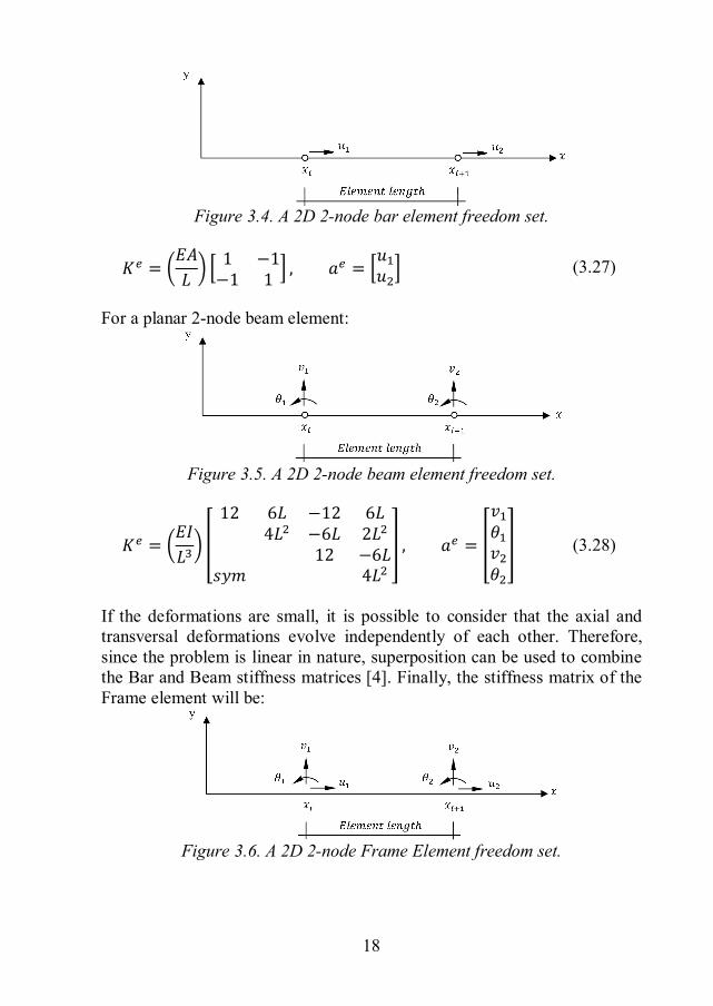
18
Figure 3.4. A 2D 2-node bar element freedom set.
퐾 =퐸퐴퐿
1 −1−1 1 , 푎 =
푢푢 (3.27)
For a planar 2-node beam element:
Figure 3.5. A 2D 2-node beam element freedom set.
퐾 =퐸퐼퐿
12 6퐿 −12 6퐿4퐿 −6퐿 2퐿
12 −6퐿푠푦푚 4퐿
, 푎 =
푣휃푣휃
(3.28)
If the deformations are small, it is possible to consider that the axial and transversal deformations evolve independently of each other. Therefore, since the problem is linear in nature, superposition can be used to combine the Bar and Beam stiffness matrices [4]. Finally, the stiffness matrix of the Frame element will be:
Figure 3.6. A 2D 2-node Frame Element freedom set.
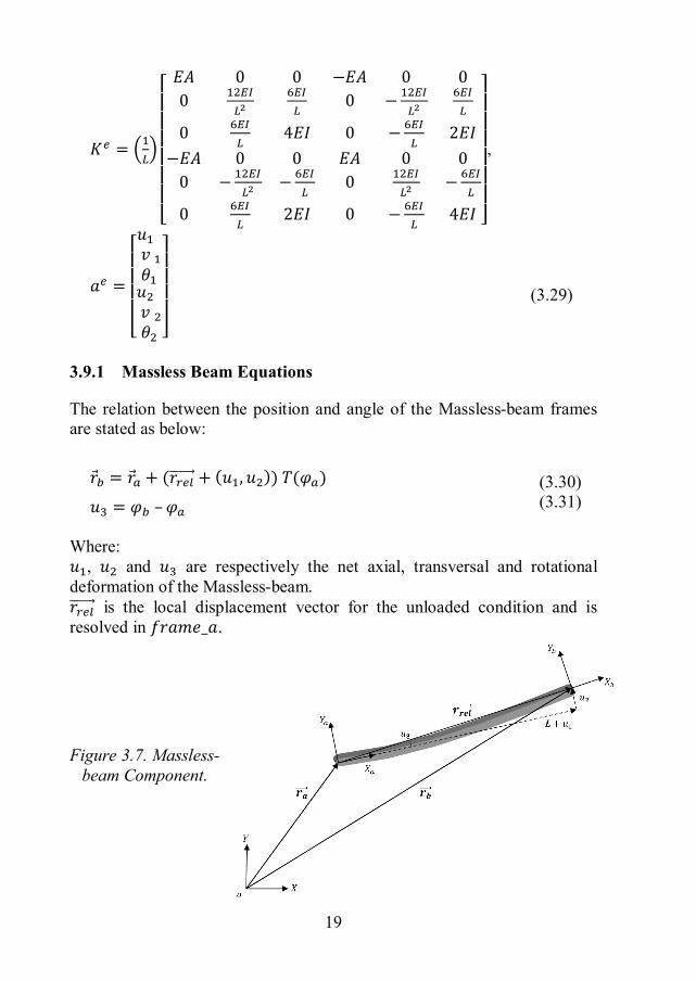
19
퐾 =
⎣⎢⎢⎢⎢⎢⎢⎡
퐸퐴 0 0 −퐸퐴 0 00 0 −
0 4퐸퐼 0 − 2퐸퐼−퐸퐴 0 0 퐸퐴 0 0
0 − − 0 −
0 2퐸퐼 0 − 4퐸퐼 ⎦⎥⎥⎥⎥⎥⎥⎤
,
푎 =
⎣⎢⎢⎢⎢⎡푢푣휃
푢푣휃 ⎦
⎥⎥⎥⎥⎤
(3.29)
3.9.1 Massless Beam Equations
The relation between the position and angle of the Massless-beam frames are stated as below:
푟 = 푟 + (푟 + (푢 , 푢 )) 푇(휑 )
푢 = 휑 – 휑 (3.30) (3.31)
Where: 푢 , 푢 and 푢 are respectively the net axial, transversal and rotational deformation of the Massless-beam. 푟 is the local displacement vector for the unloaded condition and is resolved in 푓푟푎푚푒_푎.
Figure 3.7. Massless-
beam Component.
20
The force and torque equations of the Massless-beam component are presented in equations (3.32) and (3.33).
푓 + 푓 푇(푢 ) = 0 휏 + 휏 + 푟 + (푢 , 푢 ) × (푓 푇(푢 )) = 0
(3.32) (3.33)
Because of the rotational deformation in 푓푟푎푚푒_푏, the forces in this frame are transformed to be resolved in 푓푟푎푚푒_푎’s coordinate system.
To be able to solve the above equations, the deformation values must be known. The Massless-beam component can be considered as a frame element that is fixed at one end. Therefore, by adding viscous damping as a portion of the stiffness matrix, the deformation values of the Massless-beam component can be calculated from equation (3.34).
[푓] = [퐾][푎] + [퐶][퐾][푎] (3.34)
퐶 =푐 0 00 푐 00 0 푐
, 퐾 =1퐿
⎣⎢⎢⎢⎡퐸퐴 0 0
012퐸퐼
퐿 −6퐸퐼
퐿
0 −6퐸퐼
퐿 4퐸퐼 ⎦⎥⎥⎥⎤
, 푎 =푢푢푢
푓 =푓 (푥)푓 (푦)
휏
In the above equation:
푐 and 푐 are respectively the longitudinal and the transversal damping coefficients of the beam.
The stiffness matrix [퐾] which is used in the above equation is in fact the frame element stiffness matrix whose first three rows and columns are omitted. Since the component is mass-less, the distributed load is neglected in the element force calculations. The beam material is considered as Linear Elastic in the extract of the above equations.
21
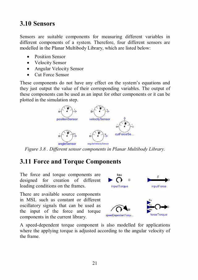
3.10 Sensors
Sensors are suitable components for measuring different variables in different components of a system. Therefore, four different sensors are modelled in the Planar Multibody Library, which are listed below:
Position Sensor Velocity Sensor Angular Velocity Sensor Cut Force Sensor
These components do not have any effect on the system’s equations and they just output the value of their corresponding variables. The output of these components can be used as an input for other components or it can be plotted in the simulation step.
Figure 3.8 . Different sensor components in Planar Multibody Library.
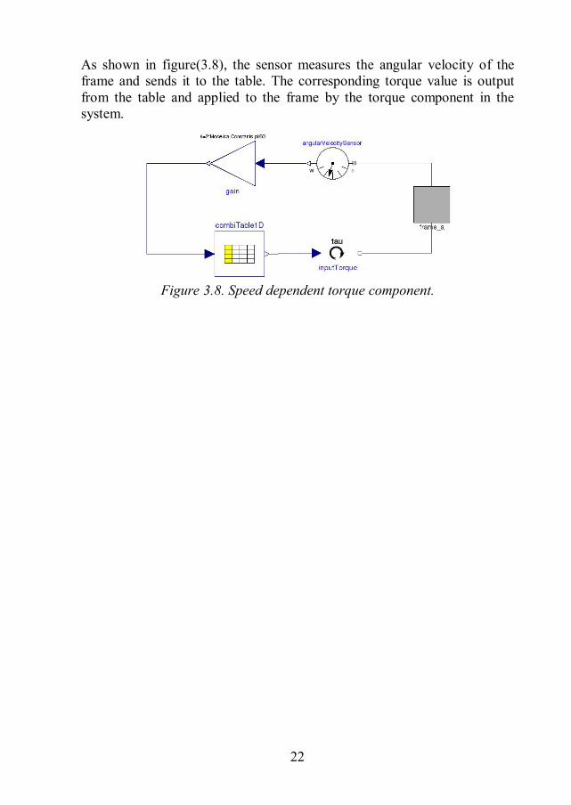
3.11 Force and Torque Components
The force and torque components are designed for creation of different loading conditions on the frames.
There are available source components in MSL such as constant or different oscillatory signals that can be used as the input of the force and torque components in the current library. A speed-dependent torque component is also modelled for applications where the applying torque is adjusted according to the angular velocity of the frame.
22
As shown in figure(3.8), the sensor measures the angular velocity of the frame and sends it to the table. The corresponding torque value is output from the table and applied to the frame by the torque component in the system.
Figure 3.8. Speed dependent torque component.
23
4 Scania Belt Drive Library
Upon completion of the Multibody Planar Library, the components can then be used for making more complex models such as Belt and Pulley components in the Scania Belt Drive Library.
4.1 Belt
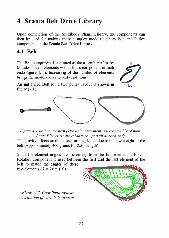
The Belt component is assumed as the assembly of many Massless-beam elements with a Mass component at each end.(Figure(4.1)). Increasing of the number of elements brings the model closer to real conditions.
An initialized Belt for a two pulley layout is shown in figure (4.1).
Figure 4.1 Belt component (The Belt component is the assembly of many
Beam Elements with a Mass component at each end). The gravity effects on the masses are neglected due to the low weight of the belt (Approximately 400 grams for 2.5m length).
Since the element angles are increasing from the first element, a Fixed-Rotation component is used between the first and the last element of the belt to match the angles of these two elements (휃 = 2푛휋 + 휃).
Figure 4.2. Coordinate system
orientation of each belt element.

24
4.2 Pulley
The Pulley is made of a Mass component which is connected to each of the Belt elements by a Contact model (Figure (4.3)).
The contact model describes the physical relationship between the pulley and belt and consist of Elastogap and Friction models; these will be explained further in the following sections.
The centre position of the pulley is connected to 푓푟푎푚푒_푎 via a revolute joint, allowing it to move and rotate freely in the plane. There is also the possibility to connect extra components such as spring, damper or friction models in the hub bearing of the pulley via the axis flanges in the revolute joint. These flanges connectors are shown by circles in the icon of the pulley.
Figure 4.3. Diagram view of Pulley component in Dymola.
25
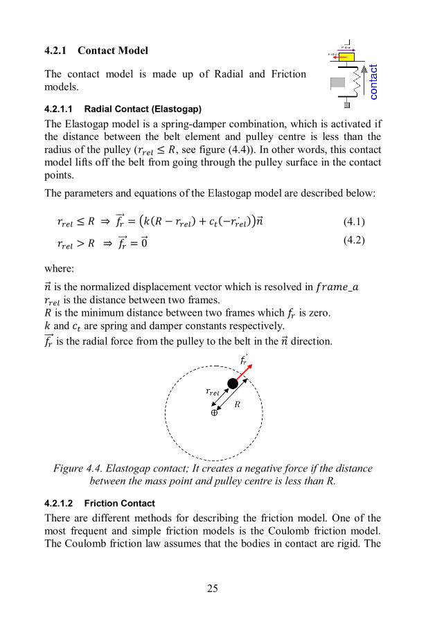
4.2.1 Contact Model
The contact model is made up of Radial and Friction models.
4.2.1.1 Radial Contact (Elastogap) The Elastogap model is a spring-damper combination, which is activated if the distance between the belt element and pulley centre is less than the radius of the pulley (푟 ≤ 푅, see figure (4.4)). In other words, this contact model lifts off the belt from going through the pulley surface in the contact points. The parameters and equations of the Elastogap model are described below:
푟 ≤ 푅 ⇒ 푓 = 푘(푅 − 푟 ) + 푐 (−푟 ) 푛
푟 > 푅 ⇒ 푓 = 0
(4.1)
(4.2)
where:
푛 is the normalized displacement vector which is resolved in 푓푟푎푚푒_푎 푟 is the distance between two frames. 푅 is the minimum distance between two frames which 푓 is zero. 푘 and 푐 are spring and damper constants respectively. 푓 is the radial force from the pulley to the belt in the 푛 direction.
Figure 4.4. Elastogap contact; It creates a negative force if the distance
between the mass point and pulley centre is less than R.
4.2.1.2 Friction Contact There are different methods for describing the friction model. One of the most frequent and simple friction models is the Coulomb friction model. The Coulomb friction law assumes that the bodies in contact are rigid. The
26
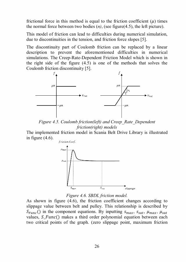
frictional force in this method is equal to the friction coefficient (휇) times the normal force between two bodies (n), (see figure(4.5), the left picture).
This model of friction can lead to difficulties during numerical simulation, due to discontinuities in the tension, and friction force slopes [5].
The discontinuity part of Coulomb friction can be replaced by a linear description to prevent the aforementioned difficulties in numerical simulations. The Creep-Rate-Dependent Friction Model which is shown in the right side of the figure (4.5) is one of the methods that solves the Coulomb friction discontinuity [5].
Figure 4.5. Coulomb friction(left) and Creep_Rate_Dependent
friction(right) models The implemented friction model in Scania Belt Drive Library is illustrated in figure (4.6).
Figure 4.6. SBDL friction model.
As shown in figure (4.6), the friction coefficient changes according to slippage value between belt and pulley. This relationship is described by 푆 () in the component equations. By inputting 푠 , 푠 , 휇 , 휇 values, 푆_퐹푢푛푐() makes a third order polynomial equation between each two critical points of the graph. (zero slippage point, maximum friction
27
point and the saturated point). The equations of the friction contact model are presented below:
푠 =|푣|
max(|푣 |, 푣 )
휇 = 푆_퐹푢푛푐(푠 , 푠 , 휇 , 휇 , 푠)
푓 = −휇 푓 푣
(4.3) (4.4)
(4.5)
Where:
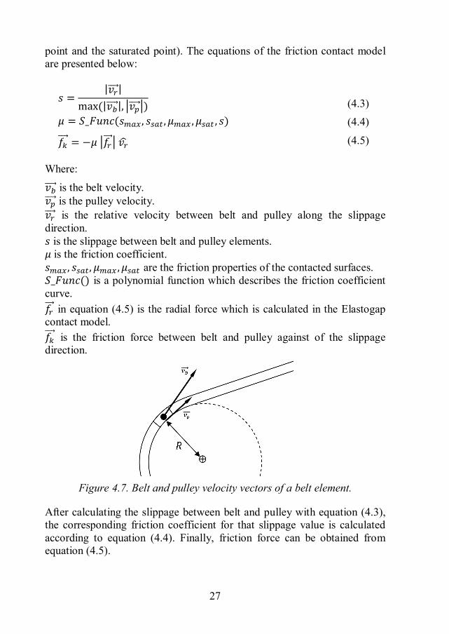
푣 is the belt velocity. 푣 is the pulley velocity. 푣 is the relative velocity between belt and pulley along the slippage direction. 푠 is the slippage between belt and pulley elements. 휇 is the friction coefficient. 푠 , 푠 , 휇 , 휇 are the friction properties of the contacted surfaces. 푆_퐹푢푛푐() is a polynomial function which describes the friction coefficient curve. 푓 in equation (4.5) is the radial force which is calculated in the Elastogap contact model. 푓 is the friction force between belt and pulley against of the slippage direction.
Figure 4.7. Belt and pulley velocity vectors of a belt element.
After calculating the slippage between belt and pulley with equation (4.3), the corresponding friction coefficient for that slippage value is calculated according to equation (4.4). Finally, friction force can be obtained from equation (4.5).
28
The belt and pulley velocity vectors in previous equations are described by equations (4.6) and (4.7). Equation (4.8) is the relative velocity between belt and pulley projected on the slippage direction.
푣 =푑푑푡 (푟)
푣 =푑푑푡 (푟) + 푅
푑푑푡 (휑 )(푒 × 푛)
푣 = (푣 . 푣 )푣 − 푣
(4.6)
(4.7)
(4.8)
Where:
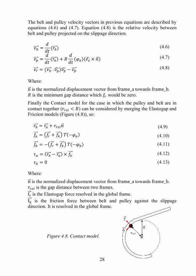
n is the normalized displacement vector from frame_a towards frame_b. 푅 is the minimum gap distance which 푓 would be zero. Finally the Contact model for the case in which the pulley and belt are in contact together (푟 < 푅) can be considered by merging the Elastogap and Friction models (Figure (4.8)), so:
푟 = 푟 + 푟 푛 (4.9)
푓 = 푓 + 푓 푇(−휑 ) (4.10)
푓 = − 푓 + 푓 푇(−휑 ) (4.11)
휏 = (푟 − 푟) × 푓 (4.12)
휏 = 0 (4.13)
Where:
n is the normalized displacement vector from frame_a towards frame_b. 푟 is the gap distance between two frames. f is the Elastogap force resolved in the global frame. f is the friction force between belt and pulley against the slippage direction. It is resolved in the global frame.
Figure 4.8. Contact model.
29
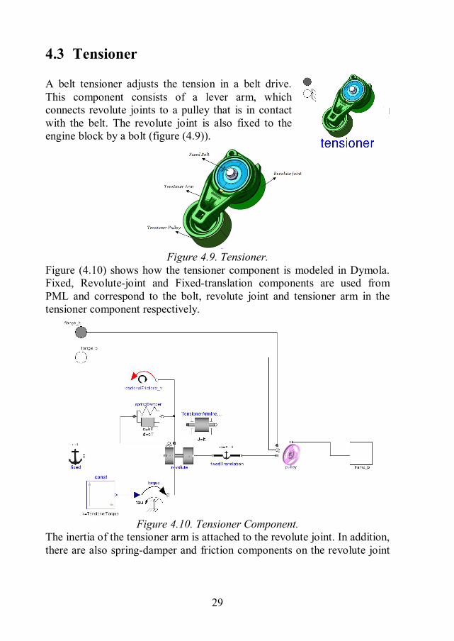
4.3 Tensioner
A belt tensioner adjusts the tension in a belt drive. This component consists of a lever arm, which connects revolute joints to a pulley that is in contact with the belt. The revolute joint is also fixed to the engine block by a bolt (figure (4.9)).
Figure 4.9. Tensioner.
Figure (4.10) shows how the tensioner component is modeled in Dymola. Fixed, Revolute-joint and Fixed-translation components are used from PML and correspond to the bolt, revolute joint and tensioner arm in the tensioner component respectively.
Figure 4.10. Tensioner Component.
The inertia of the tensioner arm is attached to the revolute joint. In addition, there are also spring-damper and friction components on the revolute joint
30
flanges. The torque component that can be seen in figure (4.10) is for creating the necessary pretension in the belt. The value of this torque is calculated by the initialization function. 4.4 Engine
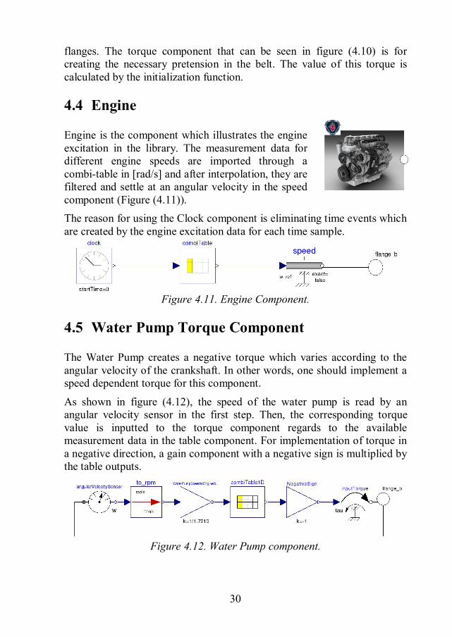
Engine is the component which illustrates the engine excitation in the library. The measurement data for different engine speeds are imported through a combi-table in [rad/s] and after interpolation, they are filtered and settle at an angular velocity in the speed component (Figure (4.11)). The reason for using the Clock component is eliminating time events which are created by the engine excitation data for each time sample.
Figure 4.11. Engine Component.
4.5 Water Pump Torque Component
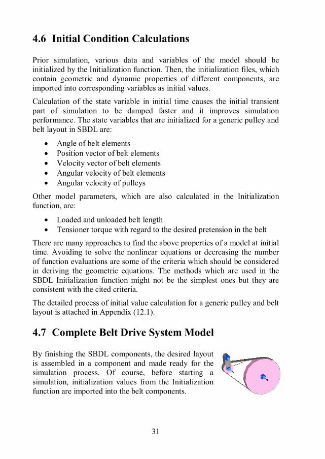
The Water Pump creates a negative torque which varies according to the angular velocity of the crankshaft. In other words, one should implement a speed dependent torque for this component.
As shown in figure (4.12), the speed of the water pump is read by an angular velocity sensor in the first step. Then, the corresponding torque value is inputted to the torque component regards to the available measurement data in the table component. For implementation of torque in a negative direction, a gain component with a negative sign is multiplied by the table outputs.
Figure 4.12. Water Pump component.
31
4.6 Initial Condition Calculations
Prior simulation, various data and variables of the model should be initialized by the Initialization function. Then, the initialization files, which contain geometric and dynamic properties of different components, are imported into corresponding variables as initial values. Calculation of the state variable in initial time causes the initial transient part of simulation to be damped faster and it improves simulation performance. The state variables that are initialized for a generic pulley and belt layout in SBDL are:
Angle of belt elements Position vector of belt elements Velocity vector of belt elements Angular velocity of belt elements Angular velocity of pulleys
Other model parameters, which are also calculated in the Initialization function, are:
Loaded and unloaded belt length Tensioner torque with regard to the desired pretension in the belt
There are many approaches to find the above properties of a model at initial time. Avoiding to solve the nonlinear equations or decreasing the number of function evaluations are some of the criteria which should be considered in deriving the geometric equations. The methods which are used in the SBDL Initialization function might not be the simplest ones but they are consistent with the cited criteria.
The detailed process of initial value calculation for a generic pulley and belt layout is attached in Appendix (12.1). 4.7 Complete Belt Drive System Model
By finishing the SBDL components, the desired layout is assembled in a component and made ready for the simulation process. Of course, before starting a simulation, initialization values from the Initialization function are imported into the belt components.
32
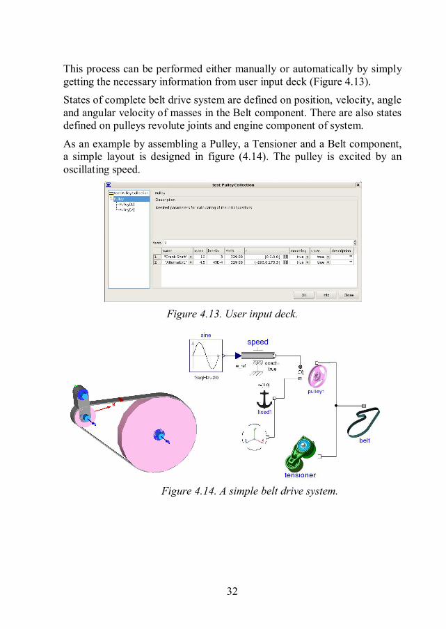
This process can be performed either manually or automatically by simply getting the necessary information from user input deck (Figure 4.13). States of complete belt drive system are defined on position, velocity, angle and angular velocity of masses in the Belt component. There are also states defined on pulleys revolute joints and engine component of system.
As an example by assembling a Pulley, a Tensioner and a Belt component, a simple layout is designed in figure (4.14). The pulley is excited by an oscillating speed.
Figure 4.13. User input deck.
Figure 4.14. A simple belt drive system.
33
5 Validation
5.1 Planar Multibody Library
The library components went continuously through a validation process. By implementing this strategy, errors were simpler to understand, compared to validation of the whole model at the end.
All the components in PML have been verified through different test examples with similar existing models in the Modelica Standard Library. It should be noticed that the components which are available in MSL are designed for three-dimensional applications. Therefore, it was not possible to use those components in SBDL and was supposed to be done a new Planar Multibody Library in this project.
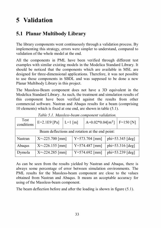
The Massless-Beam component does not have a 3D equivalent in the Modelica Standard Library. As such, the treatment and simulation results of this component have been verified against the results from other commercial software. Nastran and Abaqus results for a beam (comprising 10 elements) which is fixed at one end, are shown in table (5.1).
Table 5.1. Massless-beam component validation. Test
conditions E=2.1E9 [Pa] L=1 [m] A=0.02*0.04[푚 ] F=150 [N]
Beam deflections and rotation at the end point:
Nastran X=-225.700 [mm] Y=573.704 [mm] phi=53.345 [deg]
Abaqus X=-226.155 [mm] Y=574.487 [mm] phi=53.316 [deg]
Dymola X=-224.285 [mm] Y=574.692 [mm] phi=53.239 [deg]
As can be seen from the results yielded by Nastran and Abaqus, there is always some percentage of error between simulation environments. The PML results for the Massless-beam component are close to the values obtained from Nastran and Abaqus. It means an acceptable accuracy for using of the Massless-beam component.
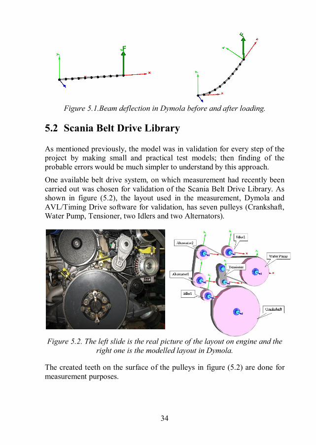
The beam deflection before and after the loading is shown in figure (5.1).
34
Figure 5.1.Beam deflection in Dymola before and after loading. 5.2 Scania Belt Drive Library
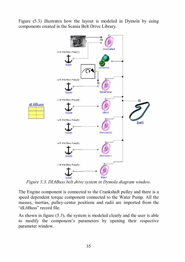
As mentioned previously, the model was in validation for every step of the project by making small and practical test models; then finding of the probable errors would be much simpler to understand by this approach. One available belt drive system, on which measurement had recently been carried out was chosen for validation of the Scania Belt Drive Library. As shown in figure (5.2), the layout used in the measurement, Dymola and AVL/Timing Drive software for validation, has seven pulleys (Crankshaft, Water Pump, Tensioner, two Idlers and two Alternators).
Figure 5.2. The left slide is the real picture of the layout on engine and the right one is the modelled layout in Dymola.
The created teeth on the surface of the pulleys in figure (5.2) are done for measurement purposes.
35
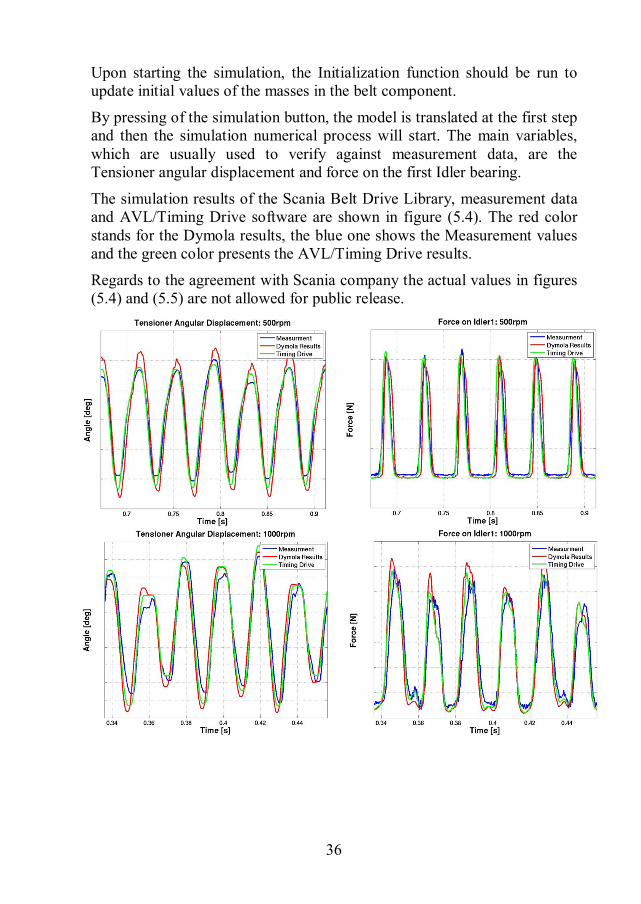
Figure (5.3) illustrates how the layout is modeled in Dymola by using components created in the Scania Belt Drive Library.
Figure 5.3. DL6Buss belt drive system in Dymola diagram window.
The Engine component is connected to the Crankshaft pulley and there is a speed dependent torque component connected to the Water Pump. All the masses, inertias, pulley-center positions and radii are imported from the “dL6Buss” record file. As shown in figure (5.3), the system is modeled clearly and the user is able to modify the component’s parameters by opening their respective parameter window.
36
Upon starting the simulation, the Initialization function should be run to update initial values of the masses in the belt component.
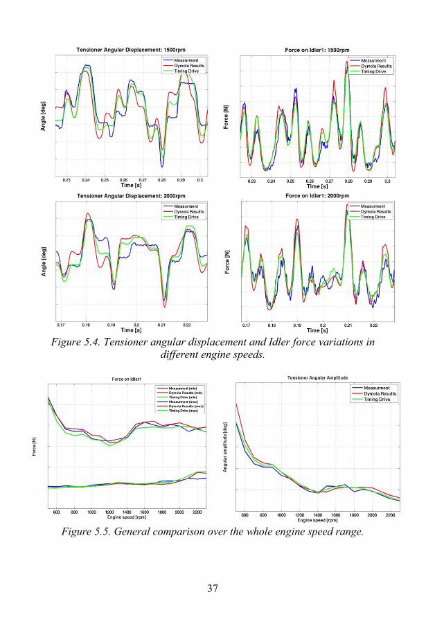
By pressing of the simulation button, the model is translated at the first step and then the simulation numerical process will start. The main variables, which are usually used to verify against measurement data, are the Tensioner angular displacement and force on the first Idler bearing.
The simulation results of the Scania Belt Drive Library, measurement data and AVL/Timing Drive software are shown in figure (5.4). The red color stands for the Dymola results, the blue one shows the Measurement values and the green color presents the AVL/Timing Drive results.
Regards to the agreement with Scania company the actual values in figures (5.4) and (5.5) are not allowed for public release.
37
Figure 5.4. Tensioner angular displacement and Idler force variations in different engine speeds.
Figure 5.5. General comparison over the whole engine speed range.
38
The maximum and minimum values of the force on the Idler1 bearing from the measurement, Dymola and AVL/Timing Drive software are collected in the same graph for different engine speeds in figure (5.5). The Tensioner angular amplitude is also plotted in a separate graph for different engine speeds in this figure. As is apparent in the graphs, there is a very good agreement between the results at different engine speeds, which is more clear in figure (5.5). With regards to criteria which are important in designing of belt drive systems, the SBDL results are promising to use for the future simulation applications in belt drive systems.
The model could be tuned and calibrated to obtain better and more matched results compared to the measured data. This process has previously been done for the AVL/Timing Drive software. The default values of different components used in SBDL are as same as the tuned AVL/Timing driving model; however since the components are not implemented in the same manner as in AVL/Timing Drive, the SBDL parameters should be tuned as well. The only difference in the model parameters compared to AVL/Timing Drive is the value of slippage at the maximum friction coefficient, which in order to match the results with measurements it was changed from 0.03 in AVL to 0.01 in SBDL. Other parameters and model properties are the same as the tuned AVL model.
The complexity of the model, sensitive parameters and model non-linearity make calibration time consuming. Performing more measurements on the components is recommended during tuning step. The most important simplifications and source of uncertainty in the model are: Parameters uncertainty:
Slippage value for the maximum friction coefficient. Longitudinal and transversal damping and stiffness of the
belt. Loads from auxiliary components
Simplified friction model. There may be some minor errors in the measurement data which
contribute to the overall error.
39
6 Performance Investigations
In the simulation performance, a try was made to make the simulation more efficient regards to time and results accuracy. There are different approaches for this purpose and in the following sections it is tried to introduce some of the major items, which effect this matter. 6.1 Selection of Integration Algorithm
The solver has a considerable effect on simulation performance. Different integration algorithms are classified according to criteria such as:
Global error One-step and multi-step algorithms Fixed and Variable step size, dense output Fixed and Variable integration order Stiff and non-stiff systems Explicit and Implicit solvers
One should not rely on just one integration algorithm in simulation experiments. Instead, selected results should be checked by two or three alternative algorithms.
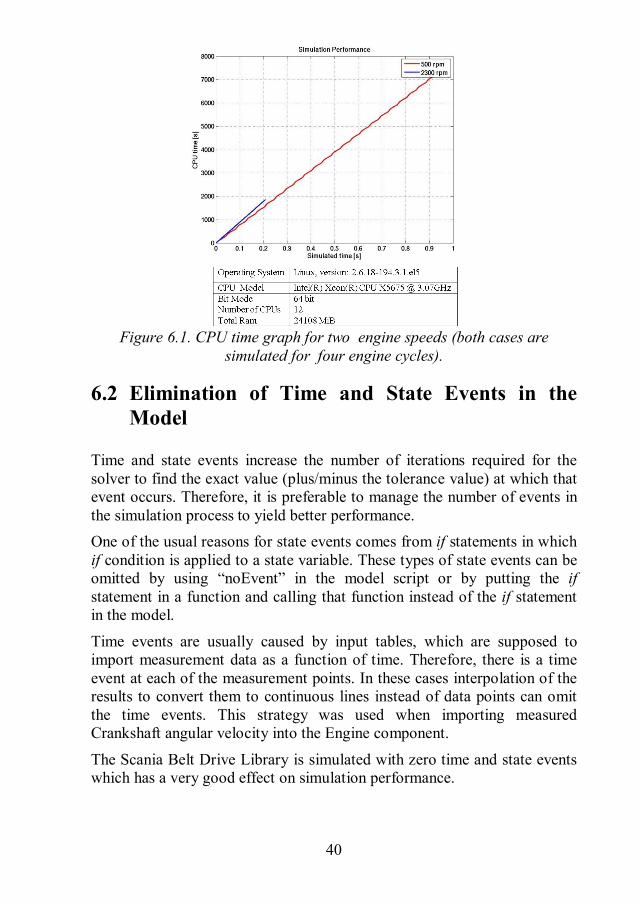
Dymosim provides a number of variable step-size integration algorithms. The solver recommended for the Scania Belt Drive Library is “Cerk23”. “Cerk23” is an explicit, non-stiff and variable step-size solver, which uses a single-step Runge-Kutta integration method. The maximum integration order of “Cerk23”is three. For the model used in the validation part, “Cerk23” was applied. With a tolerance value equals to 1E-6 and 2500 intervals (for decreasing of the polygon effect it should be more than a specific number, more information in chapter 7), all engine speeds were simulated for four engine cycles. A CPU-time graph for 500 and 2300 rpm is shown in figure (6.1). The simulation time takes about 2 hours (2.0742 hour) for 500 rpm and cirka half an hour (0.5153 hours) for 2300 rpm.
40
Figure 6.1. CPU time graph for two engine speeds (both cases are
simulated for four engine cycles).
6.2 Elimination of Time and State Events in the Model
Time and state events increase the number of iterations required for the solver to find the exact value (plus/minus the tolerance value) at which that event occurs. Therefore, it is preferable to manage the number of events in the simulation process to yield better performance. One of the usual reasons for state events comes from if statements in which if condition is applied to a state variable. These types of state events can be omitted by using “noEvent” in the model script or by putting the if statement in a function and calling that function instead of the if statement in the model.
Time events are usually caused by input tables, which are supposed to import measurement data as a function of time. Therefore, there is a time event at each of the measurement points. In these cases interpolation of the results to convert them to continuous lines instead of data points can omit the time events. This strategy was used when importing measured Crankshaft angular velocity into the Engine component.
The Scania Belt Drive Library is simulated with zero time and state events which has a very good effect on simulation performance.
41
6.3 Other Techniques
Evaluation of states with dominated error in the translation menu Omitting of unnecessary parameters in the results Choosing appropriate states can affect both accuracy and
performance simulation. Scripting component equations in an optimized manner for
decreasing the overall number of calculations and function evaluations.
Animation; simulating the model without animation or choosing simple graphical shapes such as a box instead of a beam in the beam element animation can affect simulation performance.
42
7 Polygon Effect
The Polygon effect is one of the physical effects that appears in chain drive systems. Dividing the belt into many small belt elements can be also considered as approximating the belt with a chain. This is the reason why this effect is also visible in simulation of the belt drive systems. By increasing the number of belt elements, the Polygon effect in the belt drive simulations can be decreased. It should be noted again that the Polygon effect is just a model related effect in belt drive systems so it does not occur in real conditions [6].
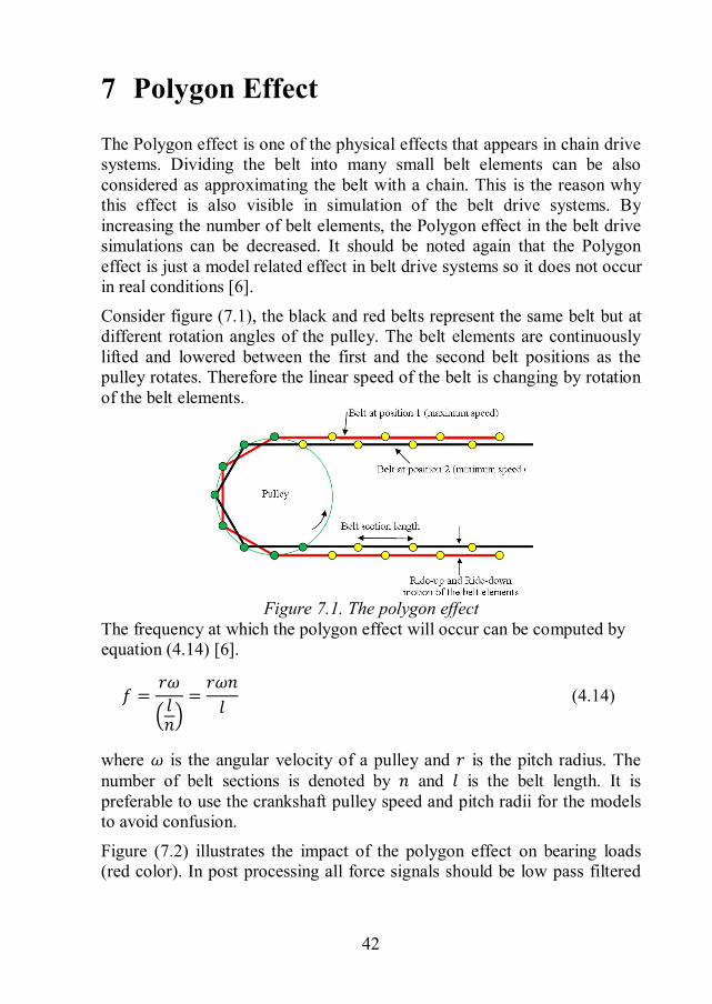
Consider figure (7.1), the black and red belts represent the same belt but at different rotation angles of the pulley. The belt elements are continuously lifted and lowered between the first and the second belt positions as the pulley rotates. Therefore the linear speed of the belt is changing by rotation of the belt elements.
Figure 7.1. The polygon effect
The frequency at which the polygon effect will occur can be computed by equation (4.14) [6].
푓 =푟휔
푙푛
=푟휔푛
푙 (4.14)
where 휔 is the angular velocity of a pulley and 푟 is the pitch radius. The number of belt sections is denoted by 푛 and 푙 is the belt length. It is preferable to use the crankshaft pulley speed and pitch radii for the models to avoid confusion.
Figure (7.2) illustrates the impact of the polygon effect on bearing loads (red color). In post processing all force signals should be low pass filtered
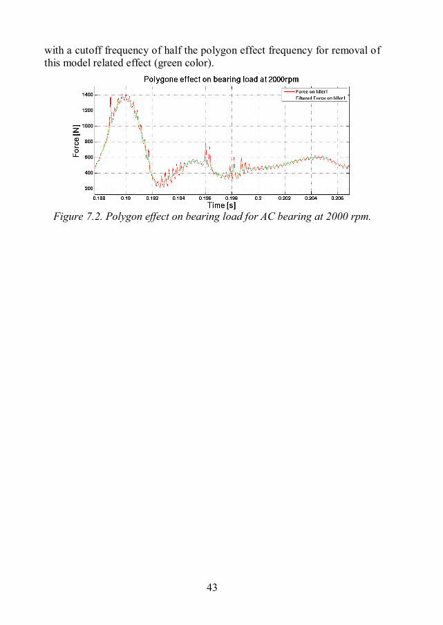
43
with a cutoff frequency of half the polygon effect frequency for removal of this model related effect (green color).
Figure 7.2. Polygon effect on bearing load for AC bearing at 2000 rpm.
44
8 Scania Belt Drive Library vs. AVL/Timing Drive
The below motivation aspects can be listed by comparing the Scania Belt Drive Library with the commercial software AVL/Timing Drive:
Cost reduction 50-75%. Access to model code Simple code implementation Less pre-processing Less error prone due to user input Simulation time Better result file naming
The below items can be considered as the drawbacks - Maintenance - Co-simulation with other software specially Power Unit - Simulation of timing belts / chains
Compared to AVL/Timing Drive, the initialization process is done within the Scania Belt Drive Library. Therefore, this possibility omits the preprocessing part before starting simulation. Simulation results are named according to the variable names which are assigned to the components. As such it would be easier to browse or compare different variables of an SBDL model in other software environments and it is no longer necessary for the user to open each of the results files to understand the corresponding component which the file belongs to.
45
9 Possible Complementary Works in Future
Calibration and Tuning of library components with regards to the uncertain parameters for matching results with measured data at all engine speeds. Performing measurement on more components of the belt drive system could make model calibration easier.
Making mass included beam elements instead of mass-less beam elements.
Inclusion of a height parameter in the belt model. The belt cord is not exactly situated at the middle of the belt width. This makes different contact length between the cord line and pulley center, if the belt is mounted from the front side or from the back side of the pulley.
Consideration of gravity effects on masses in the belt elements. Having the same length for all elements in the initialization section,
could make the initialization part more precise for the simulation start.
Post processing and results evaluation. Standard results generation. Extending the library for toothed belts or chains.

46
10 Conclusion
Advantages such as the possibility to change or update component equations, being less error prone due to user inputs and superior simulation performance are some of the major benefits of the Scania Belt Drive Library.
Comparison of results obtained with Scania Belt Drive Library with measured data and available commercial software shows a promising alternative to the current commercial software used at Scania.
47
11 References
1. Gregor Čepon1-Lionel Manin-Miha Boltežar1, (2010), Validation of a Flexible Multibody Belt-Drive Model.06,DOI:10.5545/sv-jme.2010.257
2. Dymola User Manual Volume 1, Dassault Systèmes AB.. 3. Peter Fritzson, (2003), Principles of Object-Oriented Modeling and
Simulation with Modelica 2.1, ISBN 0-471-471631. 4. Torstenfelt Bo, (2008), Finite Elements from the early beginning to the
very end, LiU-IEI-S-08/535. 5. Dooroo Kim, (2009), Dynamic Modeling of Belt Drives using the
Elastic/Perfectly-Plastic Friction Law, Georgia Institute of Technology. 6. Niklas Philipson, Method for Fixed Engine Speed Belt Drive Dynamic
Analysis, Scania Technical Report, NMBD, No. 7012546. 7. Guilhem Michon, Lionel Manin, Robert G. Parker, Régis Dufour,
(2008), Duffing Oscillator With Parametric Excitation: Analytical and Experimental Investigation on a Belt-Pulley System, DOI: 10.1115/1.2908160.
48
12 Appendix
12.1 Initialization
As it is mentioned earlier in section (4.6), the state variables that are initialized for a generic pulley and belt layout in SBDL are:
Angle of belt elements Position vector of belt elements Velocity vector of belt elements Angular velocity of belt elements Angular velocity of pulleys
Other model parameters, which are also calculated in the Initialization function, are:
Loaded and unloaded belt length Tensioner torque with regard to the desired pretension in the belt
There are many approaches to find the above properties of a model at initial time. Avoiding to solve the nonlinear equations or decreasing the number of function evaluations are some of the criteria which should be considered in deriving the geometric equations. The methods which are used in the SBDL Initialization function might not be the simplest ones but they are consistent with the cited criteria.
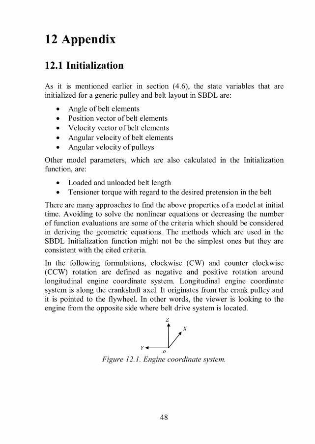
In the following formulations, clockwise (CW) and counter clockwise (CCW) rotation are defined as negative and positive rotation around longitudinal engine coordinate system. Longitudinal engine coordinate system is along the crankshaft axel. It originates from the crank pulley and it is pointed to the flywheel. In other words, the viewer is looking to the engine from the opposite side where belt drive system is located.
Figure 12.1. Engine coordinate system.
Z
Y
49
12.1.1 Link-points position vectors
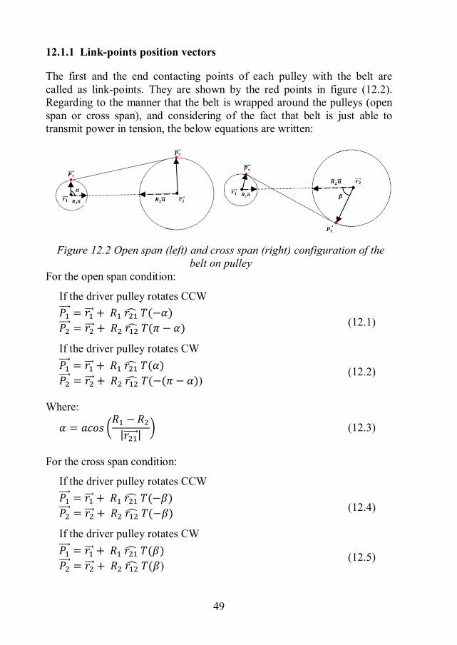
The first and the end contacting points of each pulley with the belt are called as link-points. They are shown by the red points in figure (12.2). Regarding to the manner that the belt is wrapped around the pulleys (open span or cross span), and considering of the fact that belt is just able to transmit power in tension, the below equations are written:
Figure 12.2 Open span (left) and cross span (right) configuration of the belt on pulley
For the open span condition:
If the driver pulley rotates CCW 푃 = 푟 + 푅 푟 푇(−훼) 푃 = 푟 + 푅 푟 푇(휋 − 훼) (12.1)
If the driver pulley rotates CW 푃 = 푟 + 푅 푟 푇(훼) 푃 = 푟 + 푅 푟 푇(−(휋 − 훼))
(12.2)
Where:
훼 = 푎푐표푠푅 − 푅
|푟 | (12.3)
For the cross span condition:
If the driver pulley rotates CCW 푃 = 푟 + 푅 푟 푇(−훽) 푃 = 푟 + 푅 푟 푇(−훽) (12.4)
If the driver pulley rotates CW 푃 = 푟 + 푅 푟 푇(훽) 푃 = 푟 + 푅 푟 푇(훽)
(12.5)
50
Where:
훽 = 푎푐표푠푅 + 푅
|푟 | (12.6)
This process will be looped over each two pulleys of the layout, until all the layout link-points positions are calculated.
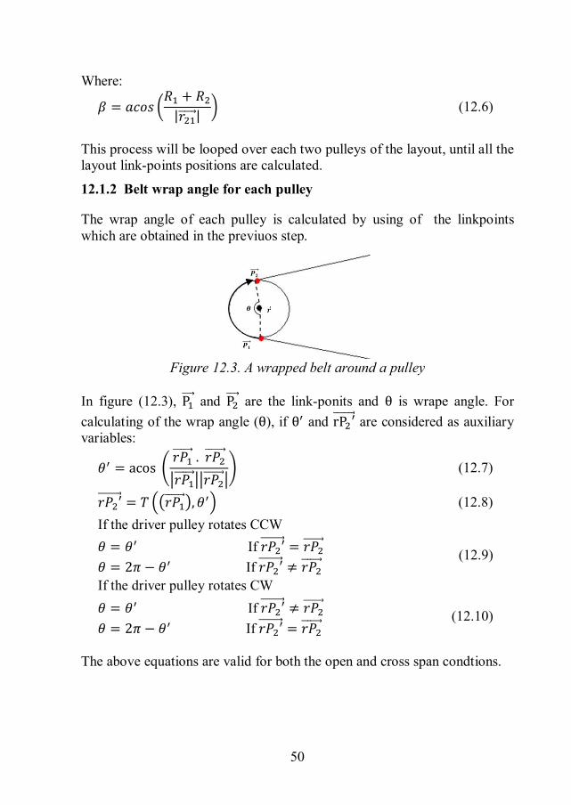
12.1.2 Belt wrap angle for each pulley
The wrap angle of each pulley is calculated by using of the linkpoints which are obtained in the previuos step.
Figure 12.3. A wrapped belt around a pulley
In figure (12.3), P and P are the link-ponits and θ is wrape angle. For calculating of the wrap angle (θ), if θ and rP ′ are considered as auxiliary variables:
휃 = acos 푟푃 . 푟푃
푟푃 푟푃 (12.7)
푟푃 ′ = 푇 푟푃 , 휃 (12.8) If the driver pulley rotates CCW 휃 = 휃 If 푟푃 ′ = 푟푃 휃 = 2휋 − 휃 If 푟푃 ′ ≠ 푟푃
(12.9)
If the driver pulley rotates CW 휃 = 휃 If 푟푃 ′ ≠ 푟푃 휃 = 2휋 − 휃 If 푟푃 ′ = 푟푃
(12.10)
The above equations are valid for both the open and cross span condtions.
51
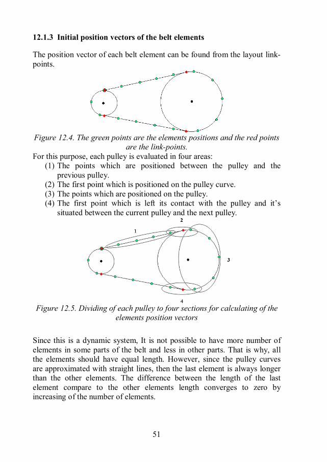
12.1.3 Initial position vectors of the belt elements
The position vector of each belt element can be found from the layout link-points.
Figure 12.4. The green points are the elements positions and the red points
are the link-points. For this purpose, each pulley is evaluated in four areas:
(1) The points which are positioned between the pulley and the previous pulley.
(2) The first point which is positioned on the pulley curve. (3) The points which are positioned on the pulley. (4) The first point which is left its contact with the pulley and it’s
situated between the current pulley and the next pulley.
Figure 12.5. Dividing of each pulley to four sections for calculating of the
elements position vectors Since this is a dynamic system, It is not possible to have more number of elements in some parts of the belt and less in other parts. That is why, all the elements should have equal length. However, since the pulley curves are approximated with straight lines, then the last element is always longer than the other elements. The difference between the length of the last element compare to the other elements length converges to zero by increasing of the number of elements.
52
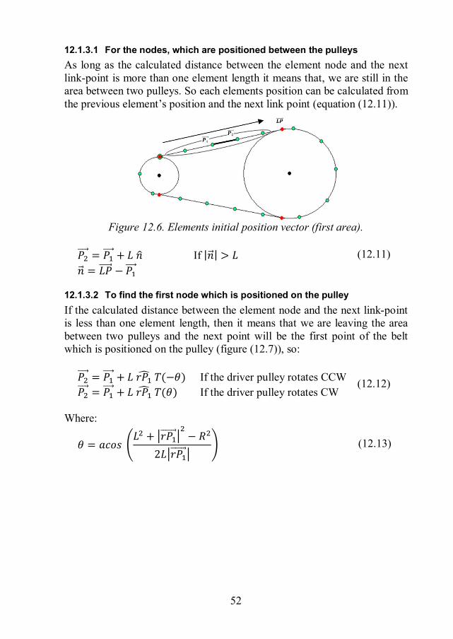
12.1.3.1 For the nodes, which are positioned between the pulleys As long as the calculated distance between the element node and the next link-point is more than one element length it means that, we are still in the area between two pulleys. So each elements position can be calculated from the previous element’s position and the next link point (equation (12.11)).
Figure 12.6. Elements initial position vector (first area).
푃 = 푃 + 퐿 푛 If |푛| > 퐿 (12.11) 푛 = 퐿푃 − 푃
12.1.3.2 To find the first node which is positioned on the pulley If the calculated distance between the element node and the next link-point is less than one element length, then it means that we are leaving the area between two pulleys and the next point will be the first point of the belt which is positioned on the pulley (figure (12.7)), so:
푃 = 푃 + 퐿 푟푃 푇(−휃) If the driver pulley rotates CCW (12.12) 푃 = 푃 + 퐿 푟푃 푇(휃) If the driver pulley rotates CW
Where:
휃 = 푎푐표푠 퐿 + 푟푃 − 푅
2퐿 푟푃 (12.13)
53
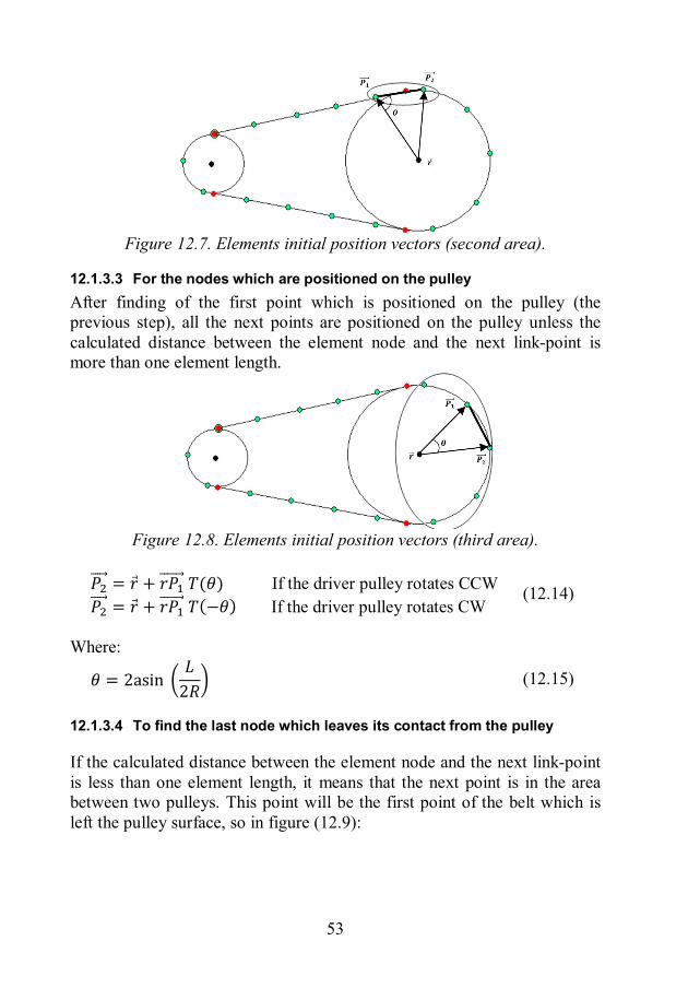
Figure 12.7. Elements initial position vectors (second area).
12.1.3.3 For the nodes which are positioned on the pulley After finding of the first point which is positioned on the pulley (the previous step), all the next points are positioned on the pulley unless the calculated distance between the element node and the next link-point is more than one element length.
Figure 12.8. Elements initial position vectors (third area).
푃 = 푟 + 푟푃 푇(휃) If the driver pulley rotates CCW (12.14) 푃 = 푟 + 푟푃 푇(−휃) If the driver pulley rotates CW
Where:
휃 = 2asin 퐿
2푅 (12.15)
12.1.3.4 To find the last node which leaves its contact from the pulley
If the calculated distance between the element node and the next link-point is less than one element length, it means that the next point is in the area between two pulleys. This point will be the first point of the belt which is left the pulley surface, so in figure (12.9):
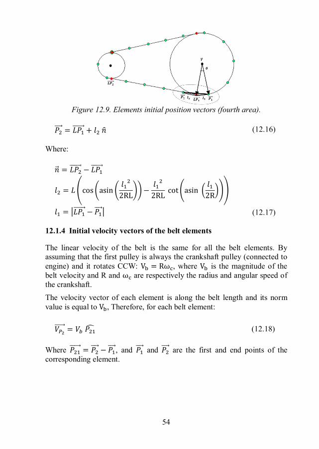
54
Figure 12.9. Elements initial position vectors (fourth area).
푃 = 퐿푃 + 푙 푛 (12.16)
Where: 푛 = 퐿푃 − 퐿푃
(12.17)
푙 = 퐿 cos asin푙
2RL −푙
2RL cot asin 푙
2R
푙 = 퐿푃 − 푃
12.1.4 Initial velocity vectors of the belt elements
The linear velocity of the belt is the same for all the belt elements. By assuming that the first pulley is always the crankshaft pulley (connected to engine) and it rotates CCW: V = Rω , where V is the magnitude of the belt velocity and R and ω are respectively the radius and angular speed of the crankshaft. The velocity vector of each element is along the belt length and its norm value is equal to V , Therefore, for each belt element:
푉 = 푉 푃 (12.18)
Where 푃 = 푃 − 푃, and 푃 and 푃 are the first and end points of the corresponding element.
55
12.1.5 Initial angle of the belt elements
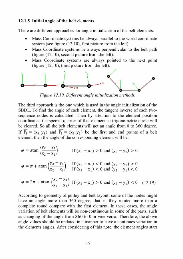
There are different approaches for angle initialization of the belt elements:
Mass Coordinate systems be always parallel to the world coordinate system (see figure (12.10), first picture from the left).
Mass Coordinate systems be always perpendicular to the belt path (figure (12.10), second picture from the left).
Mass Coordinate systems are always pointed to the next point (figure (12.10), third picture from the left).
Figure 12.10. Different angle initialization methods.
The third approach is the one which is used in the angle initialization of the SBDL. To find the angle of each element, the tangent inverse of each two-sequence nodes is calculated. Then by attention to the element position coordinates, the special quarter of that element in trigonometric circle will be cleared. So all the belt elements will get an angle from 0 to 360 degree. If P = (x , y ) and P = (x , y ) be the first and end points of a belt element then the angle of the corresponding element will be:
휑 = atany − yx − x If (x − x ) > 0 and (y − y ) > 0
(12.19)
휑 = 휋 + atany − yx − x If (x − x ) < 0 and (y − y ) > 0
If (x − x ) < 0 and (y − y ) < 0
휑 = 2휋 + atan y − yx − x If (x − x ) > 0 and (y − y ) < 0
According to geometry of pulley and belt layout, some of the nodes might have an angle more than 360 degree, that is, they rotated more than a complete round compare with the first element. In these cases, the angle variation of belt elements will be non-continuous in some of the parts, such as changing of the angle from 360 to 0 or vice versa. Therefore, the above angle values should be updated in a manner to have a continues variation in the elements angles. After considering of this note, the element angles start
56
from zero and they can have negative values or values more than 360 degree.
For compensating of the angle difference between the first and the last element, a Fixed Rotation with the corresponding angle difference is used between the first and end element of the Belt component.
12.1.6 Initial angular velocity of the pulleys
This process is started by the crankshaft angular velocity. Then the angular velocity of the next pulleys are calculated by attention to the radius ratio with the previous pulley:
ω =RR ω (12.20)
12.1.7 Initial angular velocity of the belt elements
A contact matrix has defined in the algorithm to save each of the points which are in contact with the pulleys. So the belt elements which are in contact with the pulleys are checked and then their angular velocity is considered equal to the corresponding pulley angular velocity which are calculated in the previous part. Initial angular velocities of other belt elements, which are not in contact with the pulleys, are considered equal to zero. 12.1.8 Loaded and unloaded belt length
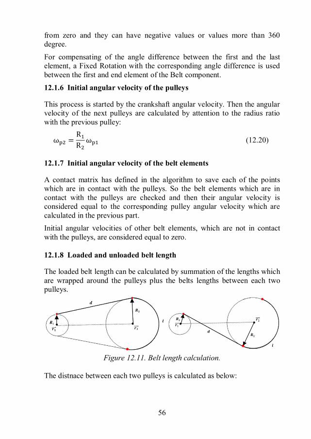
The loaded belt length can be calculated by summation of the lengths which are wrapped around the pulleys plus the belts lengths between each two pulleys.
Figure 12.11. Belt length calculation. The distnace between each two pulleys is calculated as below:
57
푑 = (|푟 푟|) − (푅 − 푅 ) Open span 푑 = (|푟 푟|) − (푅 + 푅 ) Cross span
(12.21)
The wrapped length of the belt around each pulley is obtained by: 푙 = 푅휃 Where 휃 is the wrap angle that is already calculated in previous steps.
Therefore, the total loaded belt length would be the summation of the lengths between each two pulleys (d) plus the wrapped belt lengths around of the pulleys (푙).
The unloaded belt length (퐿 ) is calculated by equation (12.22):
퐿 =퐿
1 + 퐹퐸퐴
(12.22)
Where 퐿 is the loaded belt length, 퐹 is the desire pretension in the belt and EA is the longitudinal stiffness. 12.1.9 Tensioner torque
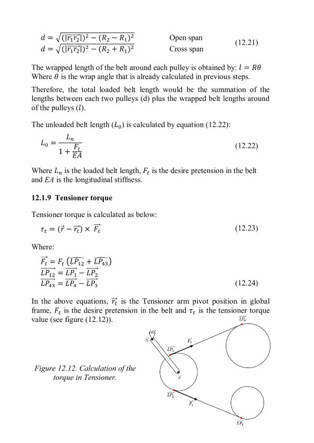
Tensioner torque is calculated as below:
휏 = (푟 − 푟 ) × 퐹 (12.23)
Where:
퐹 = 퐹 퐿푃 + 퐿푃
(12.24) 퐿푃 = 퐿푃 − 퐿푃 퐿푃 = 퐿푃 − 퐿푃
In the above equations, 푟 is the Tensioner arm pivot position in global frame, 퐹 is the desire pretension in the belt and 휏 is the tensioner torque value (see figure (12.12)).
Figure 12.12. Calculation of the torque in Tensioner.
58
12.2 SBDL User Manual
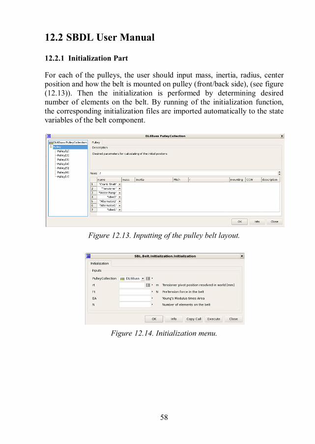
12.2.1 Initialization Part
For each of the pulleys, the user should input mass, inertia, radius, center position and how the belt is mounted on pulley (front/back side), (see figure (12.13)). Then the initialization is performed by determining desired number of elements on the belt. By running of the initialization function, the corresponding initialization files are imported automatically to the state variables of the belt component.
Figure 12.13. Inputting of the pulley belt layout.
Figure 12.14. Initialization menu.
59
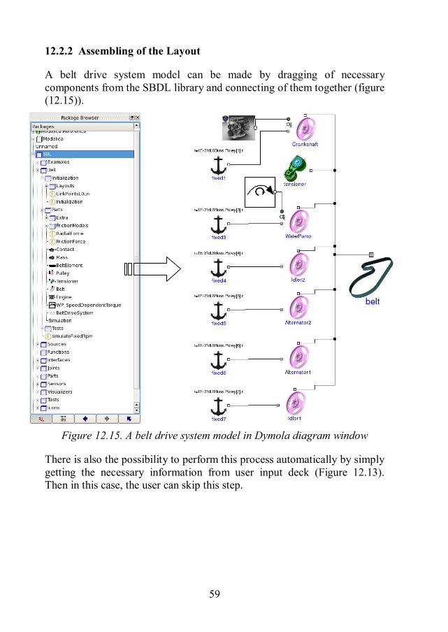
12.2.2 Assembling of the Layout
A belt drive system model can be made by dragging of necessary components from the SBDL library and connecting of them together (figure (12.15)).
Figure 12.15. A belt drive system model in Dymola diagram window
There is also the possibility to perform this process automatically by simply getting the necessary information from user input deck (Figure 12.13). Then in this case, the user can skip this step.
60
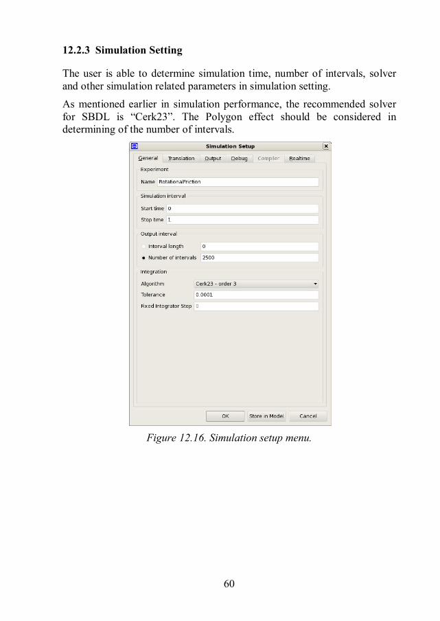
12.2.3 Simulation Setting
The user is able to determine simulation time, number of intervals, solver and other simulation related parameters in simulation setting. As mentioned earlier in simulation performance, the recommended solver for SBDL is “Cerk23”. The Polygon effect should be considered in determining of the number of intervals.
Figure 12.16. Simulation setup menu.
61
12.3 Software Environment
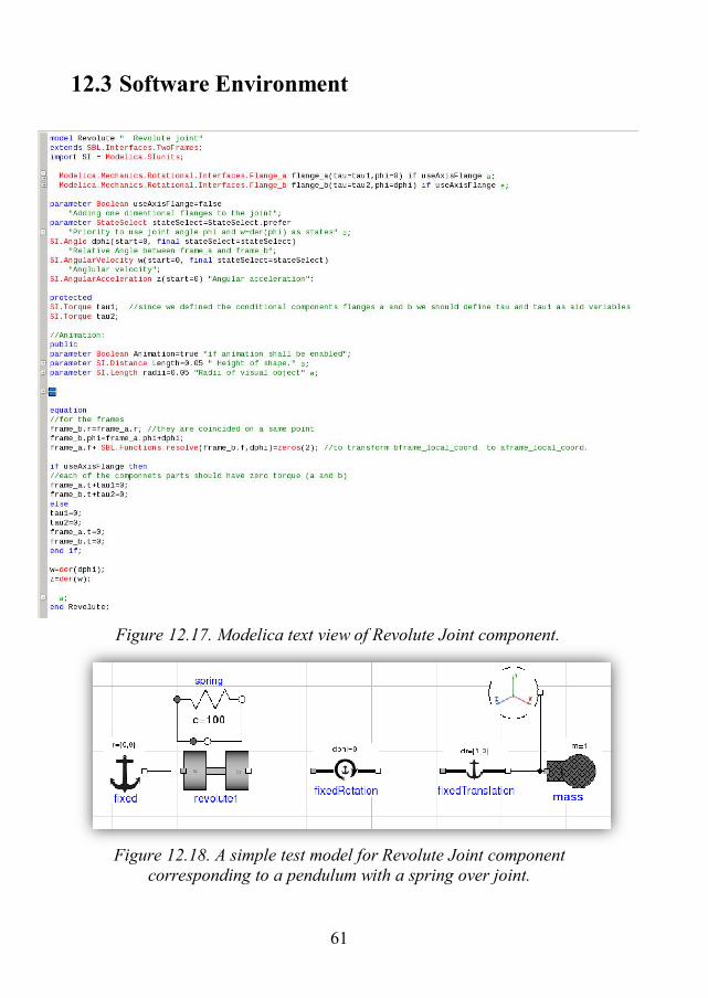
Figure 12.18. A simple test model for Revolute Joint component corresponding to a pendulum with a spring over joint.
Figure 12.17. Modelica text view of Revolute Joint component.
62
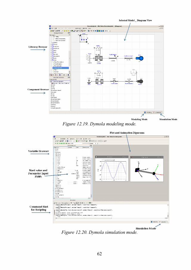
Figure 12.19. Dymola modeling mode.
Figure 12.20. Dymola simulation mode.


School of Engineering, Department of Mechanical Engineering Blekinge Institute of Technology SE-371 79 Karlskrona, SWEDEN
Telephone: E-mail:
+46 455-38 50 00 [email protected]