Embed Size (px)
Citation preview
Development, implementation and validation of software for aircraft navigation simulation
Master Thesis
Division of Automatic ControlDepartment of Electrical Engineering
Linköping University
Stefan Ahlqvist
Reg nr: LiTH-ISY-EX-3018
Supervisors: Predrag Pucar Saab ABNiclas Bergman Linköping University
Examiner: Fredrik Gustafsson Linköping University
Linköping, 1999-10-12
PrefaceThis master thesis was carried out at the section "Primary flight data and navigation" at SaabGripen in Linköping. I would like to send my appreciation to all people at Saab Gripen whohave been helpful during this thesis work. Especially, I would like to thank Mattias Lind forhelp with finding valuable background literature. Also my supervisor at Saab, Dr. PredragPucar, and my supervisor at LiTH, Dr. Niclas Bergman, deserve appreciation for their patientand well-needed support during the finishing of this report. A special thanks goes to DanielMurdin at Saab for his invaluable and patient help with the final applications in sensor fusionby Kalman filtering.
Linköping, 1999-10-12
Stefan Ahlqvist
AbstractThis thesis investigates and develops the theory necessary for implementing an aircraft simulatorwith consideration to complex aerodynamics. Furthermore the simulator is implemented andvalidated with respect to an inertial guidance system. The implementation in MathWork'sSimulink is a closed-loop system which requires development of control laws, which is done aspart of the work.
The aim is to develop a powerful environment which can be used without prior knowledge inaircraft dynamics or in-depth knowledge of Simulink. Because of this objective of user-friendliness the whole environment is controlled by a point-n'-click graphical user interface. Theevaluation of different navigational approaches can be fully performed by designing properSimulink blocks, connecting them and then setting everything up via the GUI and start thesimulation. Evaluation is also made easy as a separate data acquisition block with a GUI isprovided.
To supervise a simulation, possibility to display an aircraft-like instrument panel is implemented.The simulator environment may also be internally supervised for the possible discovery ofnumerical problems. The simulator uses terrain databases available at Saab to keep track of theground below the aircraft, both ground altitude and type of terrain.
Contents
1 Introduction 11.1 Background 11.2 Objectives 21.3 Outline 3
2 Background theory 42.1 Inertial navigation 4
2.1.1 Coordinate frames 42.1.2 Definition of position and attitude 52.1.3 Navigational equations 62.1.4 Sensors used by the INS 9
2.2 Aircraft dynamics 102.2.1 Coordinate frames used in the analysis of aircraft dynamics 102.2.2 Notation used 102.2.3 Aerodynamic forces and moments 10
2.3 Equations of motion 122.3.1 Simplifications 122.3.2 Newton's laws 132.3.3 Linear equations of motion 132.3.4 Angular equations of motion 14
2.4 Alternative navigation equations 152.4.1 Alternative velocity equation 152.4.2 Alternative position equation 162.4.3 Alternative attitude equation 16
3 Simulator construction 193.1 Implementation of the aerodynamics 193.2 Implementation of the equations of motion 223.3 Implementation of the true INS 243.4 Implementation of the alternative navigation equations 243.5 Implementation of sensor errors 253.6 Numerical solution to the differential equations 26
4 Aircraft control 274.1 Linearisation of the non-linear aerodynamics model 274.2 Guidance logic 29
4.2.1 Waypoint guidance 294.2.1.1 Course control 304.2.1.2 Altitude control 32
4.2.2 Collision avoidance guidance 334.3 Control in Waypoint navigation mode 34
4.3.1 Thrust control 344.3.2 Pitch control 354.3.3 Aileron control 374.3.4 Rudder control 38
4.4 Control in Loadfactor mode 394.4.1 Thrust control 404.4.2 Pitch control 404.4.3 Aileron control 414.4.4 Rudder control 41
5 Graphical User Interface 425.1 Flight planning tool 425.2 Other parts of the GUI 47
5.2.1 Initial state 475.2.2 Sensor Errors 475.2.3 Simulation parameters 475.2.4 Workspace output 48
5.3 Evaluation Tool 48
6 Simulator validation 496.1 Numerical stability examination 49
6.1.1 Steady level flight 496.1.2 Non-steady, non-level flight 49
6.2 Navigational validation 546.2.1 Errors in sensors parallel to the flight path 546.2.2 Errors orthogonal to the direction of travel 616.2.3 Errors resulting from attitude changes 65
7 Conclusions 707.1 Future work 71
References 72
Appendix A - Notation used
Appendix B - User's guide

Chapter 1 - Introduction 1
Chapter 1
Introduction
1.1 BackgroundThe purpose of navigation is to enable transportation of a vehicle between different points inspace. To be able to guide the vehicle, a necessity is to know where the vehicle is and in whatdirection it is heading and at what speed. This is exactly the ambition with aircraftnavigational systems, to estimate the current position and velocity.
Currently at Saab AB, a project named NINS ”New Integrated Navigation System” is underdevelopment. This project aims at improving the navigational performance of the JAS 39Gripen aircraft. An important part of this improvement lies in sensor fusion, i.e. integration ofdifferent sources of navigational information.
To be able to test navigational approaches early and at a low cost, a simulation environment isnecessary. This has been examined in earlier master theses at Saab, but these have notresulted in a complete simulation environment user-friendly and accurate enough to be usedby others than the programmers themselves. The most severe limitation of the existingsimulator is the assumption of the aircraft being a point-mass, i.e. all airflow influence isneglected. Accelerations and rotations are performed with no consideration to the limitationsof the aircraft. Also the simulation is sequential, no feedback is performed, see Figure 1.1.
Figure 1.1 - The existing INS simulator environment, with no consideration to aircraftdynamics and no feedback.
Sensor-valuescalculator
Trajectorygenerator
+
SensorErrors
AccelerationsRotations
True accelerometersTrue rate gyros
NavigationEquations
AccelerometersRate gyros
True positionTrue velocityTrue attitude
Estimated positionEstimated velocityEstimated attitude
User definedwaypoints
Chapter 1 - Introduction 2
1.2 ObjectivesThe objective of this master thesis is to construct and validate a user-friendly and accuratesimulation environment, which can be used for early evaluation of navigational algorithms.
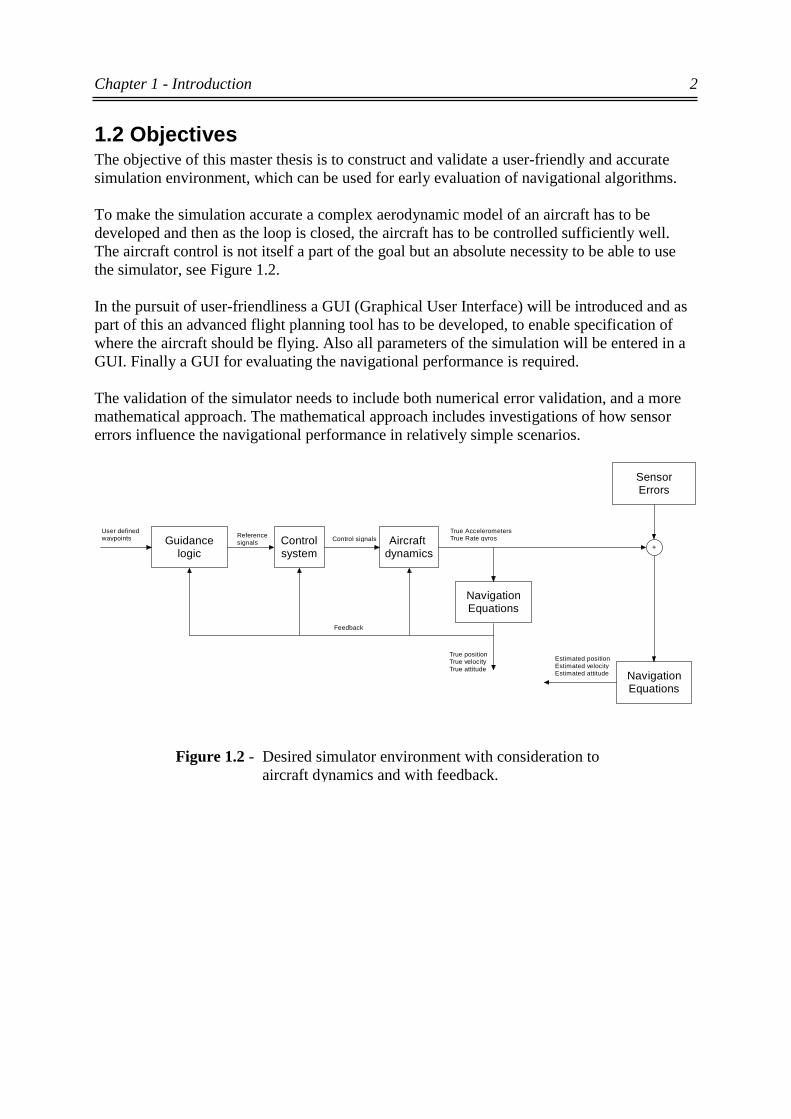
To make the simulation accurate a complex aerodynamic model of an aircraft has to bedeveloped and then as the loop is closed, the aircraft has to be controlled sufficiently well.The aircraft control is not itself a part of the goal but an absolute necessity to be able to usethe simulator, see Figure 1.2.
In the pursuit of user-friendliness a GUI (Graphical User Interface) will be introduced and aspart of this an advanced flight planning tool has to be developed, to enable specification ofwhere the aircraft should be flying. Also all parameters of the simulation will be entered in aGUI. Finally a GUI for evaluating the navigational performance is required.
The validation of the simulator needs to include both numerical error validation, and a moremathematical approach. The mathematical approach includes investigations of how sensorerrors influence the navigational performance in relatively simple scenarios.
Figure 1.2 - Desired simulator environment with consideration toaircraft dynamics and with feedback.
Guidancelogic
+
SensorErrors
Referencesignals Control signals
NavigationEquations
True AccelerometersTrue Rate gyros
True positionTrue velocityTrue attitude
Estimated positionEstimated velocityEstimated attitude
Controlsystem
Aircraft dynamics
NavigationEquations
Feedback
User definedwaypoints
Chapter 1 - Introduction 3
1.3 OutlineChapter 2 introduces the theory behind inertial navigation, aircraft dynamics and theequations of motion needed to continue the construction of the simulator. Chapter 2 alsointroduces another way of calculating the true navigational data rather than using an INS withno sensor errors. This alternative calculation is used to be able to detect numerical errors.
In Chapter 3 the implementation of the simulator and its components is discussed andsubsequently, in Chapter 4, the control of the aircraft is developed. The flight planning tooland its related components are discussed in Chapter 5. Chapter 6 contains simulator validationand Chapter 7 rounds everything up with conclusions and discussions of future work with thesimulator and related issues.
The appendices contain: (A) Notation used, (B) User's Guide to the simulator environment
Chapter 2 - Background theory 4
Chapter 2
Background theoryThis chapter discusses the background theory used in this master thesis. The ideas andcalculations behind inertial guidance, aircraft dynamics, equations of motion and the stateupdates are sorted out.
2.1 Inertial navigationThe idea of inertial navigation is to compute the actual position, velocity and attitude of amoving vehicle by using knowledge of the initial position, velocity and attitude and bymeasuring the accelerations and rotations of the vehicle. To complete these measurements, sixsensors measuring accelerations and angular velocity in an inertial reference are required.
The main problem with inertial navigation is that the position, velocity and attitude has to beintegrated from measured accelerations and rotations, which will cause constant sensor errorsto be integrated up to growing errors.
2.1.1 Coordinate framesFor the development of the INS estimates a set of coordinate frames has to be introduced.These frames are:
I - Inertial frame: A frame fixed in inertial space. This systems origin is assumed to be fixedin the centre of the earth. The z-axis of this frame is pointing out of the north pole. This is infact an approximation as the earth revolves around the sun, but this has a negligible effect onthe calculations.
E- Earth frame: A frame with its origin also fixed in the centre of the earth, but rotatingalong with the earth. The z-axis coincides with the z-axis of the I-frame. The x- and y-axes liein the equatorial plane and revolves around the z-axis once every 24 hours.
L - Local level frame: A frame with its origin at the centre of gravity of the aircraft. The z-axis always points perpendicular down through the aircraft to the surface of a referenceellipsoid described by the WGS-84 geodetic system. The NED-frame used has an x-axisalways pointing north. The y-axis points east to form a right hand orthogonal coordinateframe.
B - Body frame: A frame with its origin also in the centre of gravity of the aircraft, butrotating with the aircraft. The x-axis always points out of the nose and the y-axis alwayspoints out of the right wing. The z-axis points downwards relative to the aircraft. The INSsensors are mounted in this system and measure accelerations and rotations relative to the I-frame.
All frames but the body frame are drawn in Figure 2.1 below. The body frame is explained inthe next section. It defines the attitude of an aircraft.

Chapter 2 - Background theory 5
2.1.2 Definition of position and attitudeThe position is defined by a vector describing the aircraft latitude, longitude and altitudeabove the surface of the earth. However, as the earth is not perfectly spherical, this altitude isinstead zero-referenced by a reference ellipsoid defined by the WGS-84 geodetic system. Thevector is measured from a point that makes it perpendicular to the reference ellipsoid. Thelatitude is defined as the angle between the equatorial plane and the vector itself, and thelongitude is defined as the angle from the Greenwich meridian to the projection of theposition vector in the equatorial plane.
The attitude describes the orientation of the aircraft relative the horizontal plane, i.e. relativethe local level frame. It is defined by three angles: roll, pitch and yaw. These angles are theangles defining the difference between the body frame and the local level frame.
L
l
YL
Greeenwich meridian
Equator
ZL
XL - North
ZE, ZI
YE
XE
XI
YI
Figure 2.1 - The inertial, earth and local level frame. Latitude l, andlongitude L.
Chapter 2 - Background theory 6
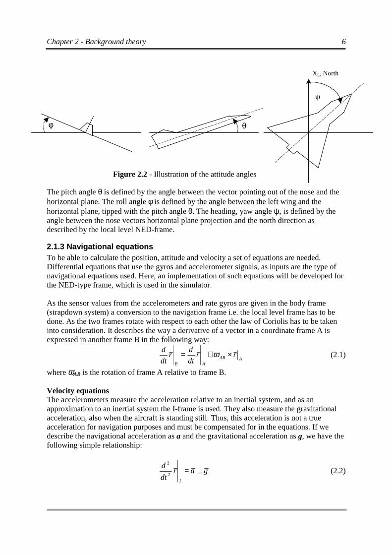
The pitch angle θ is defined by the angle between the vector pointing out of the nose and thehorizontal plane. The roll angle φ is defined by the angle between the left wing and thehorizontal plane, tipped with the pitch angle θ. The heading, yaw angle ψ, is defined by theangle between the nose vectors horizontal plane projection and the north direction asdescribed by the local level NED-frame.
2.1.3 Navigational equationsTo be able to calculate the position, attitude and velocity a set of equations are needed.Differential equations that use the gyros and accelerometer signals, as inputs are the type ofnavigational equations used. Here, an implementation of such equations will be developed forthe NED-type frame, which is used in the simulator.
As the sensor values from the accelerometers and rate gyros are given in the body frame(strapdown system) a conversion to the navigation frame i.e. the local level frame has to bedone. As the two frames rotate with respect to each other the law of Coriolis has to be takeninto consideration. It describes the way a derivative of a vector in a coordinate frame A isexpressed in another frame B in the following way:
AABAB
rrdt
dr
dt
d ×+= ω (2.1)
where ωAB is the rotation of frame A relative to frame B.
Velocity equationsThe accelerometers measure the acceleration relative to an inertial system, and as anapproximation to an inertial system the I-frame is used. They also measure the gravitationalacceleration, also when the aircraft is standing still. Thus, this acceleration is not a trueacceleration for navigation purposes and must be compensated for in the equations. If wedescribe the navigational acceleration as a and the gravitational acceleration as g, we have thefollowing simple relationship:
gardt
d
I
+=2
2
(2.2)
φ θ
ψ
Figure 2.2 - Illustration of the attitude angles
XL, North
Chapter 2 - Background theory 7
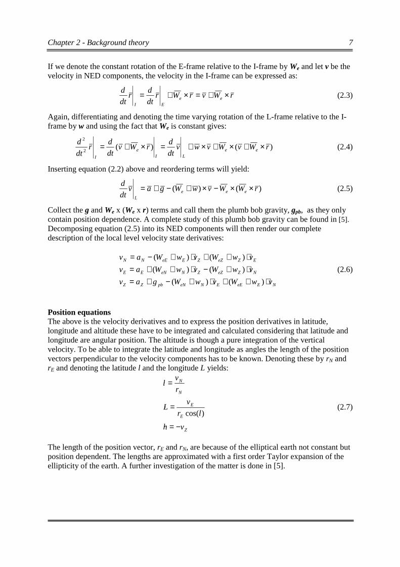
If we denote the constant rotation of the E-frame relative to the I-frame by We and let v be thevelocity in NED components, the velocity in the I-frame can be expressed as:
rWvrWrdt
dr
dt
dee
EI
×+=×+= (2.3)
Again, differentiating and denoting the time varying rotation of the L-frame relative to the I-frame by w and using the fact that We is constant gives:
)()(2
2
rWvWvwvdt
drWv
dt
dr
dt
dee
LIe
I
×+×+×+=×+= (2.4)
Inserting equation (2.2) above and reordering terms will yield:
)()( rWWvwWgavdt
deee
L
××−×+−+= (2.5)
Collect the g and We x (We x r) terms and call them the plumb bob gravity, gpb, as they onlycontain position dependence. A complete study of this plumb bob gravity can be found in [5].Decomposing equation (2.5) into its NED components will then render our completedescription of the local level velocity state derivatives:
NEeEENeNpbZZ
NZeZZNeNEE
EZeZZEeENN
vwWvwWgav
vwWvwWav
vwWvwWav
⋅++⋅+−+=⋅+−⋅++=⋅++⋅+−=
)()(
)()(
)()(
�
�
�
(2.6)
Position equationsThe above is the velocity derivatives and to express the position derivatives in latitude,longitude and altitude these have to be integrated and calculated considering that latitude andlongitude are angular position. The altitude is though a pure integration of the verticalvelocity. To be able to integrate the latitude and longitude as angles the length of the positionvectors perpendicular to the velocity components has to be known. Denoting these by rN andrE and denoting the latitude l and the longitude L yields:
Z
E
E
N
N
vh
lr
vL
r
vl
−=
=
=
�
�
�
)cos((2.7)
The length of the position vector, rE and rN, are because of the elliptical earth not constant butposition dependent. The lengths are approximated with a first order Taylor expansion of theellipticity of the earth. A further investigation of the matter is done in [5].

Chapter 2 - Background theory 8
The attitude calculation is a more complicated issue and the simulator uses two systems ofattitude calculation, the first is the transformation matrix approach used in [5]. The numericalsupervisor block in the simulator rather uses a quaternion approach, which is more numericalstable. The numerical supervisor block is discussed in Section 3.2. The reason to use twodifferent ways to calculate the attitude is to be able to detect simulation problems, i.e. whenthe two solutions start to differ, a warning will be issued.
The transformation matrix between the body frame and the local level frame (which is whatdefines the attitude) is denoted by CBL and the inverse by CLB. CBL is then used to transformvectors from the B-frame to the L-frame.
=
−⋅
−⋅
−=
333231
232221
131211
cossin0
sincos0
001
cos0sin
010
sin0cos
100
0cossin
0sincos
ccc
ccc
ccc
CBL
φφφφ
θθ
θθψψψψ
(2.8)
As we only need to keep track of three angles and this matrix contains 9 elements, the matrixhas to obey six conditions to be correct. The solution with quaternions only has 4 elementsand will then only have to obey one condition and that is also the explanation to why it ismore numerically stable. The 6 conditions are that the vectors representing the rows must beorthonormalised, i.e. they have to be perpendicular to each other and have unity magnitude.An improvement made to previous versions of the simulator is to improve the simulationperformance by performing the Gram-Schmidt orthonormalisation process at each integrationstep.
To obtain the desired Euler attitude angles from the transformation matrix above, use:
=
−−=
=
33
32
31
31
11
21
atan2
1atan
atan2
2
c
c
c
c
c
c
φ
θ
ψ
(2.9)
The atan2 function is a four quadrant inverse tangent, it will yield an answer in the domain-π< atan2(x) <π for all real x. It considers the signs of the nominator and denominator of x todecide which domain to use. Now, remembering that the measurements provided by the INSsensors is the rotation with respect to inertial space, i.e. the I-frame, gives the possibility torewrite the matrix as:
BIILBL CCC = (2.10)
Differentiating gives:
BIILBIILBL CCCCC ��� += (2.11)
Chapter 2 - Background theory 9
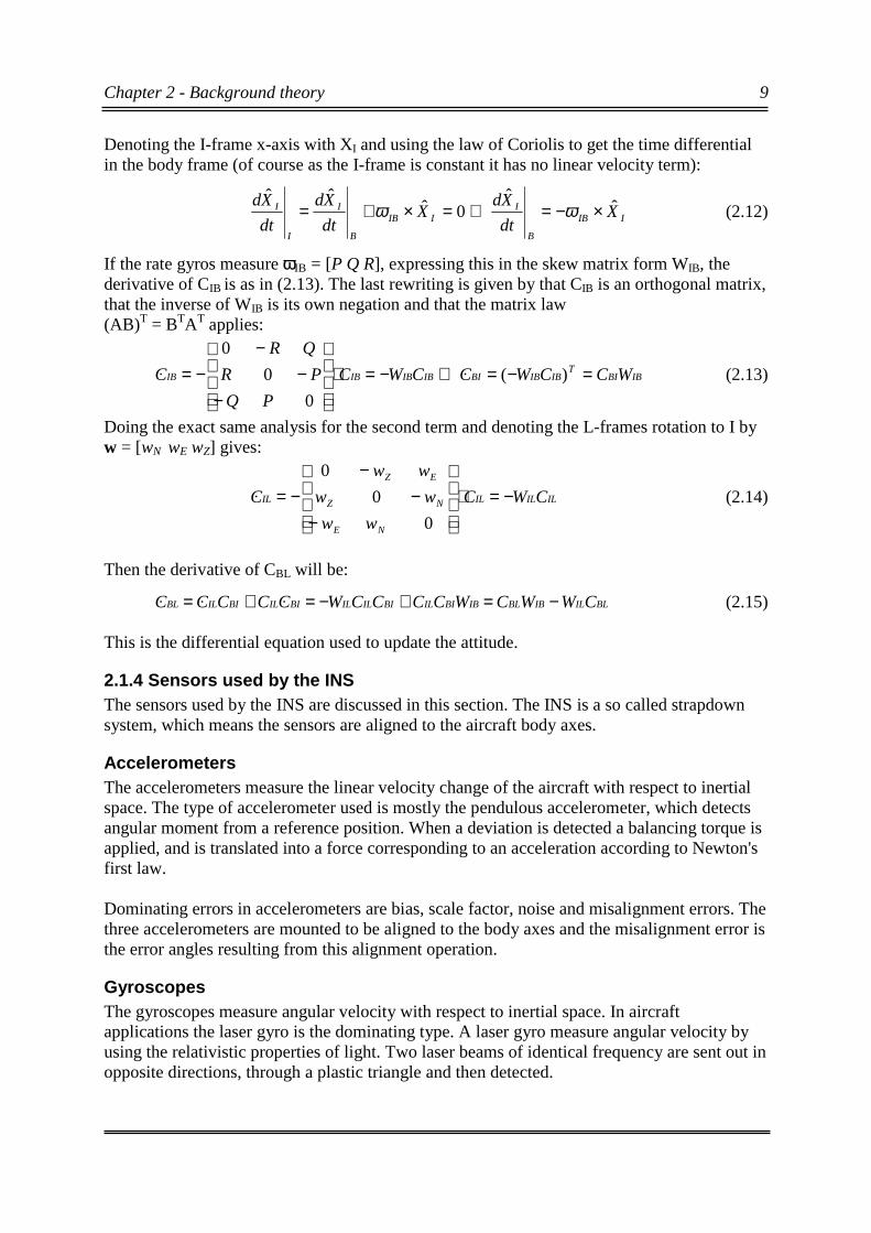
Denoting the I-frame x-axis with XI and using the law of Coriolis to get the time differentialin the body frame (of course as the I-frame is constant it has no linear velocity term):
IIB
B
IIIB
B
I
I
I Xdt
XdX
dt
Xd
dt
Xd ˆˆ
0ˆˆˆ
×−=⇒=×+= ωω (2.12)
If the rate gyros measure ωIB = [P Q R], expressing this in the skew matrix form WIB, thederivative of CIB is as in (2.13). The last rewriting is given by that CIB is an orthogonal matrix,that the inverse of WIB is its own negation and that the matrix law(AB)T = BTAT applies:
IBBIT
IBIBBIIBIBIBIB WCCWCCWC
PQ
PR
QR
C =−=⇒−=⋅
−−
−−= )(
0
0
0�� (2.13)
Doing the exact same analysis for the second term and denoting the L-frames rotation to I byw = [wN wE wZ] gives:
ILILIL
NE
NZ
EZ
IL CWC
ww
ww
ww
C −=⋅
−−
−−=
0
0
0� (2.14)
Then the derivative of CBL will be:
BLILIBBLIBBIILBIILILBIILBIILBL CWWCWCCCCWCCCCC −=+−=+= ��� (2.15)
This is the differential equation used to update the attitude.
2.1.4 Sensors used by the INSThe sensors used by the INS are discussed in this section. The INS is a so called strapdownsystem, which means the sensors are aligned to the aircraft body axes.
AccelerometersThe accelerometers measure the linear velocity change of the aircraft with respect to inertialspace. The type of accelerometer used is mostly the pendulous accelerometer, which detectsangular moment from a reference position. When a deviation is detected a balancing torque isapplied, and is translated into a force corresponding to an acceleration according to Newton'sfirst law.
Dominating errors in accelerometers are bias, scale factor, noise and misalignment errors. Thethree accelerometers are mounted to be aligned to the body axes and the misalignment error isthe error angles resulting from this alignment operation.
GyroscopesThe gyroscopes measure angular velocity with respect to inertial space. In aircraftapplications the laser gyro is the dominating type. A laser gyro measure angular velocity byusing the relativistic properties of light. Two laser beams of identical frequency are sent out inopposite directions, through a plastic triangle and then detected.
Chapter 2 - Background theory 10
On detection the two beams will differ in frequency if the aircraft is rotating. This frequencydifference can then be transformed into an angular velocity.
The dominating errors of the gyroscopes are the same as for the accelerometers.
2.2 Aircraft dynamicsThe wind flow against the aircraft body produces forces and moments, resulting in linear andangular accelerations of the aircraft. The dynamic model developed will describe these effectsand also describe pilot-controlled effects on the aircraft such as control surface deflectionsand engine thrust. First, as background theory, a general discussion of aircraft dynamics willbe presented.
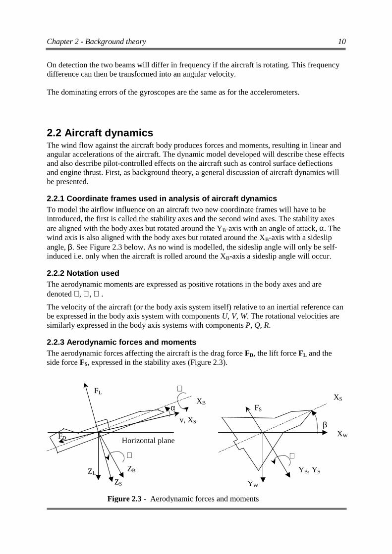
2.2.1 Coordinate frames used in analysis of aircraft dynamicsTo model the airflow influence on an aircraft two new coordinate frames will have to beintroduced, the first is called the stability axes and the second wind axes. The stability axesare aligned with the body axes but rotated around the YB-axis with an angle of attack, α. Thewind axis is also aligned with the body axes but rotated around the XB-axis with a sideslipangle, β. See Figure 2.3 below. As no wind is modelled, the sideslip angle will only be self-induced i.e. only when the aircraft is rolled around the XB-axis a sideslip angle will occur.
2.2.2 Notation usedThe aerodynamic moments are expressed as positive rotations in the body axes and aredenoted ℑ, ℜ, ℘.
The velocity of the aircraft (or the body axis system itself) relative to an inertial reference canbe expressed in the body axis system with components U, V, W. The rotational velocities aresimilarly expressed in the body axis systems with components P, Q, R.
2.2.3 Aerodynamic forces and momentsThe aerodynamic forces affecting the aircraft is the drag force FD, the lift force FL and theside force FS, expressed in the stability axes (Figure 2.3).
XB
β
XS
XW
YB, YS
YW
ℜ
v, XS
α
ZS
FL
FD Horizontal plane
ZB
℘
ZL
ℑ
FS
Figure 2.3 - Aerodynamic forces and moments
Chapter 2 - Background theory 11
The aerodynamic forces and moments are modelled by functions dependent on different statevariables such as the angle of attack α, sideslip angle β, airspeed, control surface deflections δetc.
Denoting the current state (velocity, rotation and position) by x and denoting the controlsurface deflections δ (δa aileron, δr rudder, δe elevator and δT thrust control) this approachgives us the appropriate forces and moments aerodynamic coefficients to be used as:
),(
),(
),(
),(
),(
),(
δδδ
δ
δ
δ
xfC
xfC
xfC
xfC
xfC
xfC
SS
DD
LL
FF
FF
FF
℘℘
ℜℜ
ℑℑ
=
=
=
=
=
=
(2.16)
The coefficients are mainly dependent on the attack angle, airspeed and control surfacedeflections. Each control surface has a primary influence and other minor influences upon theaircraft. This is discussed in the linearisation of a few equilibrium points in Section 4.1. Alsosome damping factors are present, which are mainly dependent on the rotations performed bythe aircraft.
One traditional way of describing these functions is to describe all wind derivatives (a way ofexpressing the aerodynamics of an aircraft) and from these calculate all forces and momentscoefficients. This is the approach described in [1]. In this simulator another method was usedas aerodynamic data on the F-16 fighter aircraft was available, from the development of anearlier tactical simulator environment at Saab.
The functions in (2.16) are, of course, different for different types of aircraft. In the simulatorthe functions developed are based on the aerodynamics of the F-16 fighter aircraft. In generalsuch functions are determined by performing wind tunnel tests and other experiments with theaircraft, often resulting in a function including table lookups and damping terms. This is alsothe case for this simulator. An older simulation environment developed in Fortran at Saab ABprovided the functions used. These functions were expressed directly in the body frame butcan, of course, be calculated into the stability axes if needed.
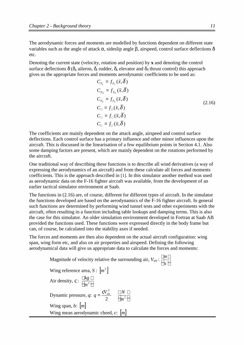
The forces and moments are then also dependent on the actual aircraft configuration: wingspan, wing form etc, and also on air properties and airspeed. Defining the followingaerodynamical data will give us appropriate data to calculate the forces and moments:
Magnitude of velocity relative the surrounding air, Vair :
s
m
Wing reference area, S : [ ]2m
Air density, ς :
3m
kg
Dynamic pressure, q:
=
2
2
2 m
NVq airς
Wing span, b: [ ]m
Wing mean aerodynamic chord, c: [ ]m
Chapter 2 - Background theory 12
These data are then combined with the coefficients from equations (2.16) and this yields:
℘
ℜ
ℑ
=℘
=ℜ
=ℑ
−=
−=
−=
∑∑∑∑∑∑
SqbC
SqcC
SqbC
SqCF
SqCF
SqCF
S
D
L
FS
FD
FL
(2.17)
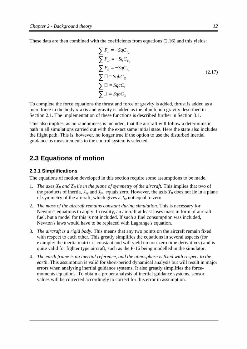
To complete the force equations the thrust and force of gravity is added, thrust is added as amere force in the body x-axis and gravity is added as the plumb bob gravity described inSection 2.1. The implementation of these functions is described further in Section 3.1.
This also implies, as no randomness is included, that the aircraft will follow a deterministicpath in all simulations carried out with the exact same initial state. Here the state also includesthe flight path. This is, however, no longer true if the option to use the disturbed inertialguidance as measurements to the control system is selected.
2.3 Equations of motion
2.3.1 SimplificationsThe equations of motion developed in this section require some assumptions to be made.
1. The axes XB and ZB lie in the plane of symmetry of the aircraft. This implies that two ofthe products of inertia, Jxy and Jyz, equals zero. However, the axis YB does not lie in a planeof symmetry of the aircraft, which gives a Jxz not equal to zero.
2. The mass of the aircraft remains constant during simulation. This is necessary forNewton's equations to apply. In reality, an aircraft at least loses mass in form of aircraftfuel, but a model for this is not included. If such a fuel consumption was included,Newton's laws would have to be replaced with Lagrange's equation.
3. The aircraft is a rigid body. This means that any two points on the aircraft remain fixedwith respect to each other. This greatly simplifies the equations in several aspects (forexample: the inertia matrix is constant and will yield no non-zero time derivatives) and isquite valid for fighter type aircraft, such as the F-16 being modelled in the simulator.
4. The earth frame is an inertial reference, and the atmosphere is fixed with respect to theearth. This assumption is valid for short-period dynamical analysis but will result in majorerrors when analysing inertial guidance systems. It also greatly simplifies the force-moments equations. To obtain a proper analysis of inertial guidance systems, sensorvalues will be corrected accordingly to correct for this error in assumption.
Chapter 2 - Background theory 13
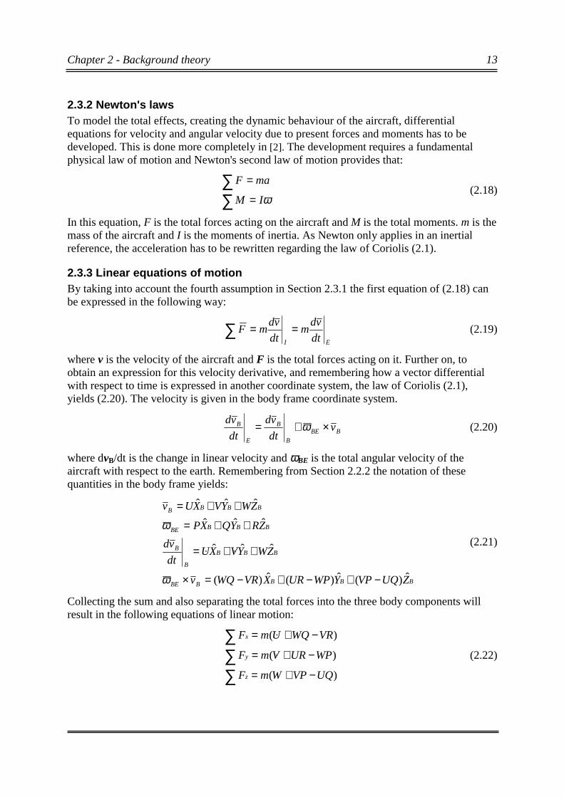
2.3.2 Newton's lawsTo model the total effects, creating the dynamic behaviour of the aircraft, differentialequations for velocity and angular velocity due to present forces and moments has to bedeveloped. This is done more completely in [2]. The development requires a fundamentalphysical law of motion and Newton's second law of motion provides that:
∑∑
=
=
ω�IM
maF (2.18)
In this equation, F is the total forces acting on the aircraft and M is the total moments. m is themass of the aircraft and I is the moments of inertia. As Newton only applies in an inertialreference, the acceleration has to be rewritten regarding the law of Coriolis (2.1).
2.3.3 Linear equations of motionBy taking into account the fourth assumption in Section 2.3.1 the first equation of (2.18) canbe expressed in the following way:
EI dt
vdm
dt
vdmF ==∑ (2.19)
where v is the velocity of the aircraft and F is the total forces acting on it. Further on, toobtain an expression for this velocity derivative, and remembering how a vector differentialwith respect to time is expressed in another coordinate system, the law of Coriolis (2.1),yields (2.20). The velocity is given in the body frame coordinate system.
BBE
B
B
E
B vdt
vd
dt
vd×+= ω (2.20)
where dvB/dt is the change in linear velocity and ωBE is the total angular velocity of theaircraft with respect to the earth. Remembering from Section 2.2.2 the notation of thesequantities in the body frame yields:
BBBBBE
BBB
B
B
BBBBE
BBBB
ZUQVPYWPURXVRWQv
ZWYVXUdt
vd
ZRYQXP
ZWYVXUv
ˆ)(ˆ)(ˆ)(
ˆˆˆ
ˆˆˆ
ˆˆˆ
−+−+−=×
++=
++=
++=
ω
ω
���(2.21)
Collecting the sum and also separating the total forces into the three body components willresult in the following equations of linear motion:
)(
)(
)(
UQVPWmF
WPURVmF
VRWQUmF
z
y
x
−+=
−+=
−+=
∑∑∑
�
�
�
(2.22)
Chapter 2 - Background theory 14
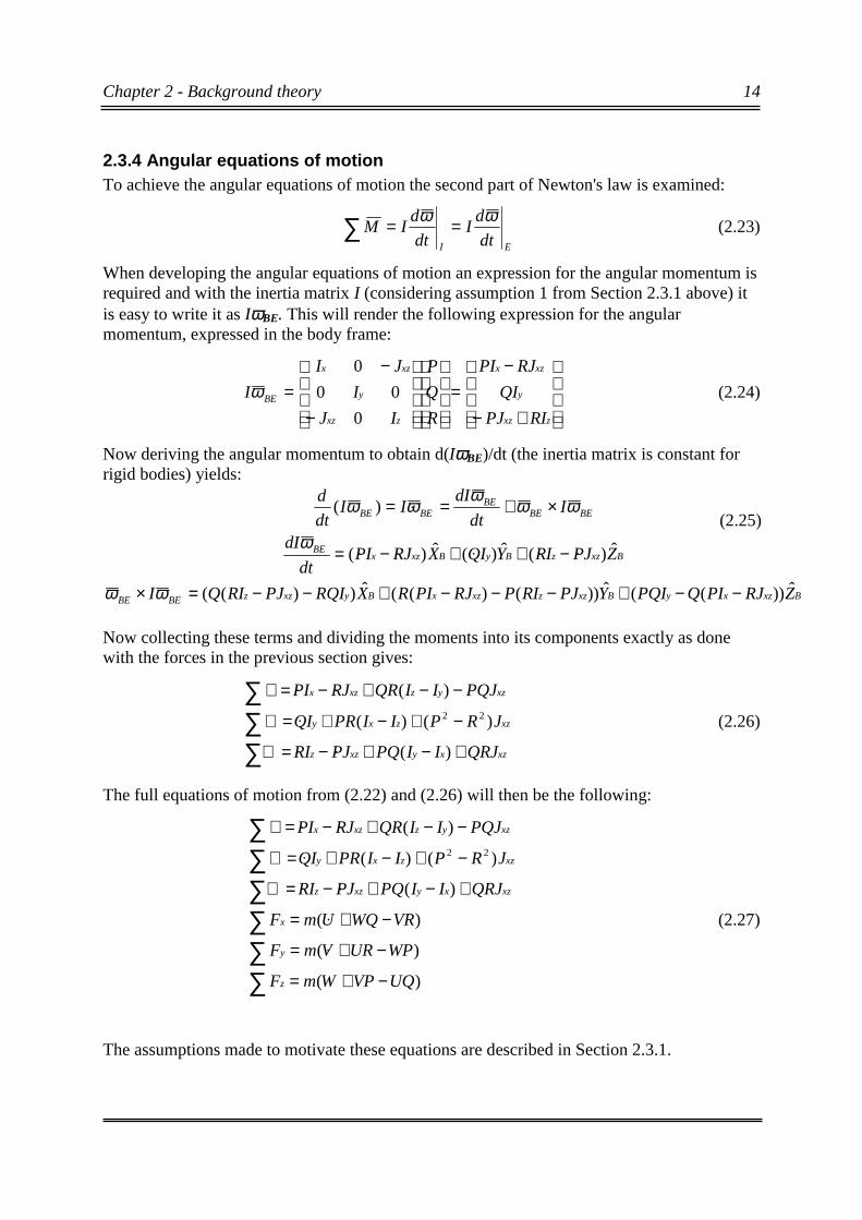
2.3.4 Angular equations of motionTo achieve the angular equations of motion the second part of Newton's law is examined:
EI dt
dI
dt
dIM
ωω ==∑ (2.23)
When developing the angular equations of motion an expression for the angular momentum isrequired and with the inertia matrix I (considering assumption 1 from Section 2.3.1 above) itis easy to write it as IωBE. This will render the following expression for the angularmomentum, expressed in the body frame:
+−
−=
−
−=
zxz
y
xzx
zxz
y
xzx
BE
RIPJ
QI
RJPI
R
Q
P
IJ
I
JI
I
0
00
0
ω (2.24)
Now deriving the angular momentum to obtain d(IωBE)/dt (the inertia matrix is constant forrigid bodies) yields:
BxzxyBxzzxzxByxzzBEBE
BxzzByBxzxBE
BEBEBE
BEBE
ZRJPIQPQIYPJRIPRJPIRXRQIPJRIQI
ZJPIRYIQXJRIPdt
dI
Idt
dIII
dt
d
ˆ))((ˆ))()((ˆ))((
ˆ)(ˆ)(ˆ)(
)(
−−+−−−+−−=×
−++−=
×+==
ωω
ω
ωωωωω
�����
�
Now collecting these terms and dividing the moments into its components exactly as donewith the forces in the previous section gives:
xzxyxzz
xzzxy
xzyzxzx
QRJIIPQJPIR
JRPIIPRIQ
PQJIIQRJRIP
+−+−=℘
−+−+=ℜ
−−+−=ℑ
∑∑∑
)(
)()(
)(22
��
�
��
(2.26)
The full equations of motion from (2.22) and (2.26) will then be the following:
)(
)(
)(
)(
)()(
)(22
UQVPWmF
WPURVmF
VRWQUmF
QRJIIPQJPIR
JRPIIPRIQ
PQJIIQRJRIP
z
y
x
xzxyxzz
xzzxy
xzyzxzx
−+=
−+=
−+=
+−+−=℘
−+−+=ℜ
−−+−=ℑ
∑∑∑∑∑∑
�
�
�
��
�
��
(2.27)
The assumptions made to motivate these equations are described in Section 2.3.1.
(2.25)

Chapter 2 - Background theory 15
Now to be able to update the state, the state derivatives have to be solved for in (2.27) and thisoperation gives:
∑
∑
∑∑
∑
∑
∑
ℜ+−−−−=
+−−+ℑ=
−
+−−ℑ+℘=
+−=
+−=
+−=
yy
xzzx
xzyzxzx
x
xzz
x
xzyz
x
xz
x
xz
z
y
x
II
JRPIIPRQ
PQJIIQRJRI
P
I
JI
PQI
JIIQR
I
J
I
J
R
Fm
VPUQW
Fm
URWPV
Fm
WQVRU
1)()(
))((1
)(
1
1
1
22
2
2
�
��
�
�
�
�
(2.28)
Note that the P differential includes the R differential, the expression for the R differentialcould be inserted directly instead. These equations are then integrated at each step in thesimulation to obtain the new state.
2.4 Alternative navigation equationsIn Section 2.3 a way of determining the update of linear and angular velocity in the bodyframe was developed, but this is not enough. In an inertial guidance system both position andattitude is calculated and to evaluate these the true position and attitude are also needed. Thisis of course also true for all other navigational algorithms to be tested, a truth to compare withis needed. In fact, in the simulator, this will be solved in two ways. First a true INS is used,i.e. an INS with no sensor errors, and to back this up another set of navigation equations, notusing sensor data but rather simulation internal values (i.e. direct use of dvB/dt and P Q R), areused. The latter will be developed in this chapter.
2.4.1 Alternative velocity equationRecalling that the internal state included states for the aircraft velocity expressed in bodycoordinates (U, V, W), only a conversion of this speed to the local frame has to be done. Thisis made with the Euler angles representing the aircraft attitude. This will yield:
L
L
LL
BBBB
ZWVU
YWVU
XWVUv
ZWYVXUv
ˆ)coscoscossinsin(
ˆ))cossinsinsin(cos)sinsinsincos(cossincos(
ˆ))cossincossin(sin)sincoscossin(sincoscos(
ˆˆˆ
θφθφθ
ψφψθφψθφψφψθ
ψθφψφψφψθφψθ
−−+
−++++
++−+=
++=
This gives us the true aircraft velocity expressed in the local frame. This approach has a majordeficiency also, as Euler angles are not defined when pitch is +/- π/2. This is not taken care ofin the simulator but will only rarely cause not desired numerical warnings as such attitudesnever occurs in the waypoint mode.
(2.29)
Chapter 2 - Background theory 16
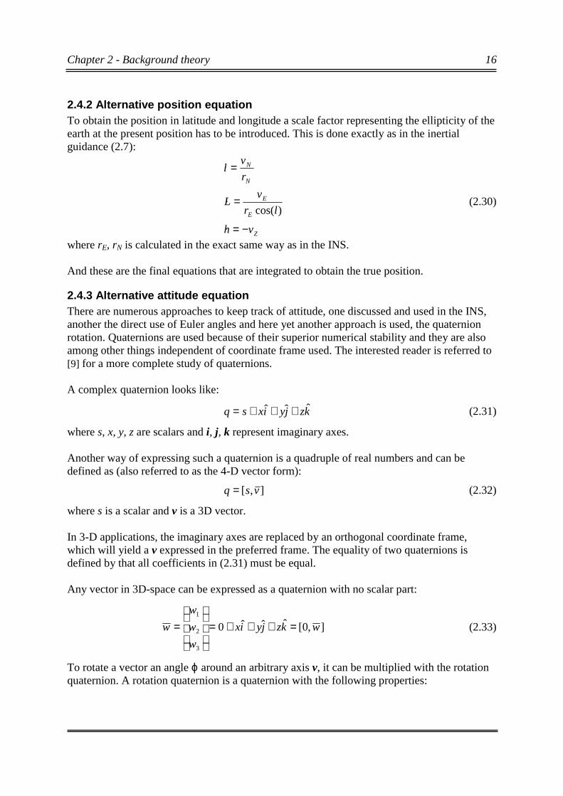
2.4.2 Alternative position equationTo obtain the position in latitude and longitude a scale factor representing the ellipticity of theearth at the present position has to be introduced. This is done exactly as in the inertialguidance (2.7):
Z
E
E
N
N
vh
lr
vL
r
vl
−=
=
=
�
�
�
)cos((2.30)
where rE, rN is calculated in the exact same way as in the INS.
And these are the final equations that are integrated to obtain the true position.
2.4.3 Alternative attitude equationThere are numerous approaches to keep track of attitude, one discussed and used in the INS,another the direct use of Euler angles and here yet another approach is used, the quaternionrotation. Quaternions are used because of their superior numerical stability and they are alsoamong other things independent of coordinate frame used. The interested reader is referred to[9] for a more complete study of quaternions.
A complex quaternion looks like:
kzjyixsq ˆˆˆ +++= (2.31)
where s, x, y, z are scalars and i, j, k represent imaginary axes.
Another way of expressing such a quaternion is a quadruple of real numbers and can bedefined as (also referred to as the 4-D vector form):
],[ vsq = (2.32)
where s is a scalar and v is a 3D vector.
In 3-D applications, the imaginary axes are replaced by an orthogonal coordinate frame,which will yield a v expressed in the preferred frame. The equality of two quaternions isdefined by that all coefficients in (2.31) must be equal.
Any vector in 3D-space can be expressed as a quaternion with no scalar part:
],0[ˆˆˆ0
3
2
1
wkzjyix
w
w
w
w =+++=
= (2.33)
To rotate a vector an angle ϕ around an arbitrary axis v, it can be multiplied with the rotationquaternion. A rotation quaternion is a quaternion with the following properties:

Chapter 2 - Background theory 17
]sin,[cos
]sin,[cos
1
1
2222
ϕϕϕϕ
vq
vq
zyxsq
−==
=+++=
−
(2.34)
A multiplication of quaternions is defined as (q1 and q2 quaternions of the form (2.32))
]),[( 211221212121 vvvsvsvsssqq ×++•−= (2.35)
If the vector w is expressed as a quaternion as in (2.33) and multiplied by the rotationquaternion q and its inverse as from (2.34),
1' −= qwqw (2.36)
it will result in a new quaternion w', rotated ϕ degrees around the axis v, which also can beexpressed as a normal 3D vector, if the scalar part (which is zero for all vectors) of thequaternion is ignored.
A single rotation quaternion with these four degrees of freedom will thereby include allinformation needed to transform vectors between the body frame and the local level frame.This can be compared to the approach the CBL-matrix, which has 9 degrees of freedom. Thismeans the quaternion only has to obey the condition of being a unity quaternion, whilst theCBL matrix must obey the six conditions of orthonormality (three for unity vector in rows andthree for the orthogonality of the three rows).
The complex quaternion is expressed in the 4-D vector form, which makes the body framecontain the complex axes. This makes the quaternion rotation be expressed in the same frameas the calculated angular velocity (P, Q, R) in Section 2.2. A complex quaternion in 4-D form(from (2.32)) looks like:
)sin,(cos)ˆ,ˆ,ˆ,( 3210 ϕϕ vkqjqiqqq == (2.37)
where (i, j, k) is the orthonormal body axes, v is the axis of rotation (unity magnitude)expressed in body axes, and ϕ is the rotation angle.
The initial state is declared in Euler angles, and to use the quaternion approach this initialstate has to be transformed into quaternions which is done with following formula:
−
=
+
=
−
=
+
=
2cos
2sin
2sin
2sin
2cos
2cos
2sin
2cos
2sin
2cos
2sin
2cos
2sin
2sin
2cos
2cos
2cos
2sin
2sin
2sin
2sin
2cos
2cos
2cos
3
2
1
0
ψθφψθφ
ψθφψθφ
ψθφψθφ
ψθφψθφ
q
q
q
q
(2.38)
Chapter 2 - Background theory 18
The four quaternions used are then updated with the following differential equations:
2
)(2
)(2
)(2
)(
2103
3102
3201
3210
qPqQqRq
qPqRqQq
qQqRqPq
qRqQqPq
⋅+⋅−⋅−−=
⋅−⋅+⋅−−=
⋅+⋅−⋅−−=
⋅+⋅+⋅−=
�
�
�
�
(2.39)
The Euler attitude angles are then calculated by the following formulas:
( ))(2sina
)(22atan
)(22atan
2031
23
2210
1032
23
2210
3021
22
22
qqqq
qqqq
qqqq
qqqq
qqqq
⋅−⋅−=
+−−⋅+⋅
=
−−+⋅+⋅
=
θ
φ
ψ
(2.40)
These are the equations used to determine the true state of the aircraft in the numericalsupervisor circuit which is used to detect numerical errors in the simulation.

Chapter 3 - Simulator implementation 19
Chapter 3
Simulator constructionThe simulator environment was developed in MatLab / Simulink provided by MathWorksInc. The Simulink environment was chosen on the following basis:
• The simplicity, everything in the simulator is treated as signals.• All blocks are separated, which means any aerodynamics can be introduced into the system
by only replacing the Aircraft Dynamics block (i.e. wind models, other aircraft etc). Thesame applies for the control system, to replace it only the corresponding blocks have to bereplaced.
• Very little code has to be written (and later understood by others).• All blocks can be considered to be black boxes with inputs and outputs. This makes it
easier to use, the user only has to see what is adequate for his/her needs. Any navigationalapproach can be evaluated without even opening the Navigation Simulator block. Also infuture work, every part system of the navigation aims to be incorporated into one block andfrom this view, sensor fusion algorithms are easy to implement and evaluate.
• The speed, Simulink offers a higher speed in simulation as everything can be effectivelyimplemented without need for the MatLab interpreter.
3.1 Implementation of the aerodynamicsThe aerodynamics block consists of three parts, first a hydraulics & engine system to simulatecontrol surface delay and engine dynamics, secondly a calculation of all aerodynamic forcesand moments and lastly a calculation of outputted sensor values relative to the systems toperform the integrations in.
Hydraulics & engine systemThe hydraulic system is approximated with first-order transfer function models. The thrust isapproximated with two different transfer functions, one to describe ordinary thrust andanother to describe the afterburner effect. A step input of 105 kN (which is maximum thrustwith afterburner for the F-16) is shown in Figure 3.1.
0 1 2 3 4 5 60
2
4
6
8
10
12x 10
4 Thrust com m anded m aximal (105kN) at t im e = 1 s
Tim e [s ]
Th
rus
t p
ow
er
[N]
Figure 3.1 - Engine dynamics
Chapter 3 - Simulator implementation 20
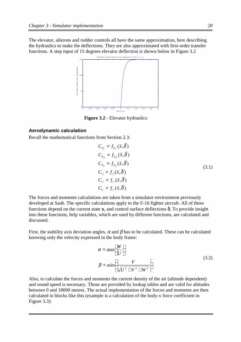
The elevator, ailerons and rudder controls all have the same approximation, here describingthe hydraulics to make the deflections. They are also approximated with first-order transferfunctions. A step input of 15 degrees elevator deflection is shown below in Figure 3.2
Aerodynamic calculationRecall the mathematical functions from Section 2.3:
),(
),(
),(
),(
),(
),(
δδδ
δ
δ
δ
xfC
xfC
xfC
xfC
xfC
xfC
SS
DD
LL
FF
FF
FF
℘℘
ℜℜ
ℑℑ
=
=
=
=
=
=
(3.1)
The forces and moments calculations are taken from a simulator environment previouslydeveloped at Saab. The specific calculations apply to the F-16 fighter aircraft. All of thesefunctions depend on the current state x, and control surface deflections δ. To provide insightinto these functions, help variables, which are used by different functions, are calculated anddiscussed.
First, the stability axis deviation angles, α and β has to be calculated. These can be calculatedknowing only the velocity expressed in the body frame:
++=
=
222asin
atan
WVU
V
U
W
β
α
(3.2)
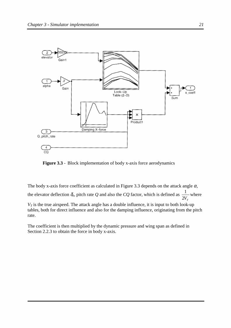
Also, to calculate the forces and moments the current density of the air (altitude dependent)and sound speed is necessary. Those are provided by lookup tables and are valid for altitudesbetween 0 and 18000 metres. The actual implementation of the forces and moments are thencalculated in blocks like this (example is a calculation of the body-x force coefficient inFigure 3.3):
0 0 . 2 0 . 4 0 . 6 0 . 8 1 1 . 2 1 . 4 1 . 6 1 . 8 20
5
1 0
1 5E le va t o r s t e p in p u t o f 1 5 d e g re e s a t t im e = 1 s
T im e [ s ]
Ele
vato
r d
efl
ec
tio
n [
de
gre
es
]
Figure 3.2 - Elevator hydraulics
Chapter 3 - Simulator implementation 21
The body x-axis force coefficient as calculated in Figure 3.3 depends on the attack angle α,
the elevator deflection δe, pitch rate Q and also the CQ factor, which is defined as TV2
1where
VT is the true airspeed. The attack angle has a double influence, it is input to both look-uptables, both for direct influence and also for the damping influence, originating from the pitchrate.
The coefficient is then multiplied by the dynamic pressure and wing span as defined inSection 2.2.3 to obtain the force in body x-axis.
Figure 3.3 - Block implementation of body x-axis force aerodynamics
Chapter 3 - Simulator implementation 22
Also remembering from Section 2.2 the forces are functions of different aircraft and airparameters:
℘
ℜ
ℑ
=℘
=ℜ
=ℑ
−=
−=
−=
∑∑∑∑∑∑
SqbC
SqcC
SqbC
SqCF
SqCF
SqCF
S
D
L
FS
FD
FL
(3.3)
When this is done the plumb bob gravity described in Section 2.1 is added, it is actually takenfrom the true INS which is part of the simulator and then transformed into body framecoordinates.
These are the calculations made and all forces and moments are put into one vector going outto the calculation of the equations of motion.
3.2 Implementation of the equations of motionIn Section 2.3 the full equations of motion were developed when approximating an inertialframe with the E-frame:
)(
)(
)(
)(
)()(
)(22
UQVPWmF
WPURVmF
VRWQUmF
QRJIIPQJPIR
JRPIIPRIQ
PQJIIQRJRIP
z
y
x
xzxyxzz
xzzxy
xzyzxzx
−+=
−+=
−+=
+−+−=℘
−+−+=ℜ
−−+−=ℑ
∑∑∑∑∑∑
�
�
�
��
�
��
(3.4)
The forces and moments output from the aerodynamics section are due to the assumption ofthe E-frame as an inertial frame, expressed in the B-frame relative to the E-frame. But as therotation caused by the aircraft moving above the surface of the elliptical earth is not modelledin the aircraft dynamics section, the output values can be seen as relative to the local levelframe. This yields that the [P Q R] elements above describe the actual angular velocity of theB-frame relative to the L-frame. The state derivatives for the angular velocities are calculatedexactly as stated in Section 2.3 and is as follows:

Chapter 3 - Simulator implementation 23
∑
∑
∑∑
ℜ+−−−−=
+−−+ℑ=
−
+−−ℑ+℘=
yy
xzzx
xzyzxzx
x
xzz
x
xzyz
x
xz
x
xz
II
JRPIIPRQ
PQJIIQRJRI
P
I
JI
PQI
JIIQR
I
J
I
J
R
1)()(
))((1
)(
2
2
�
��
�
(3.5)
These are then integrated to get the [P Q R] rotation vector.
Also, this yields that the velocity state derivatives in the B-frame can be calculatedstraightforward exactly as stated in the equations below:
∑
∑
∑
+−=
+−=
+−=
z
y
x
Fm
VPUQW
Fm
URWPV
Fm
WQVRU
1
1
1
�
�
�
(3.6)
When calculated these rotation derivatives and accelerations are put through to theNavigational Equations block which integrates the equations from Section 2.4.
Sensor outputsAgain, consider that the model output was expressed in the B-frame relative to the local levelframe and that the inertial guidance system in the simulator approximates the inertial framewith the I-frame not the E-frame. This yields that accelerations and angular velocities have tobe modified with the rotation wIL , the rotation of the L-frame relative to the I-frame. Theaccelerations need to be modified with the Coriolis acceleration resulting from this rotation.
( ) BILLBLBIB
ILLBIB
VwCaa
www
×+=+=
⋅(3.7)
All rotations referred to in these equations are originally expressed in the local level NEDframe. The rotation of the local level frame relative to the I-frame is taken and transformedinto body coordinates from the true INS in the simulator. This rotation consists of the E-frames rotation around the I-frame We and the L-frames rotation due to the aircraft movingaround the non-planar earth. The expressions below are taken from [5]
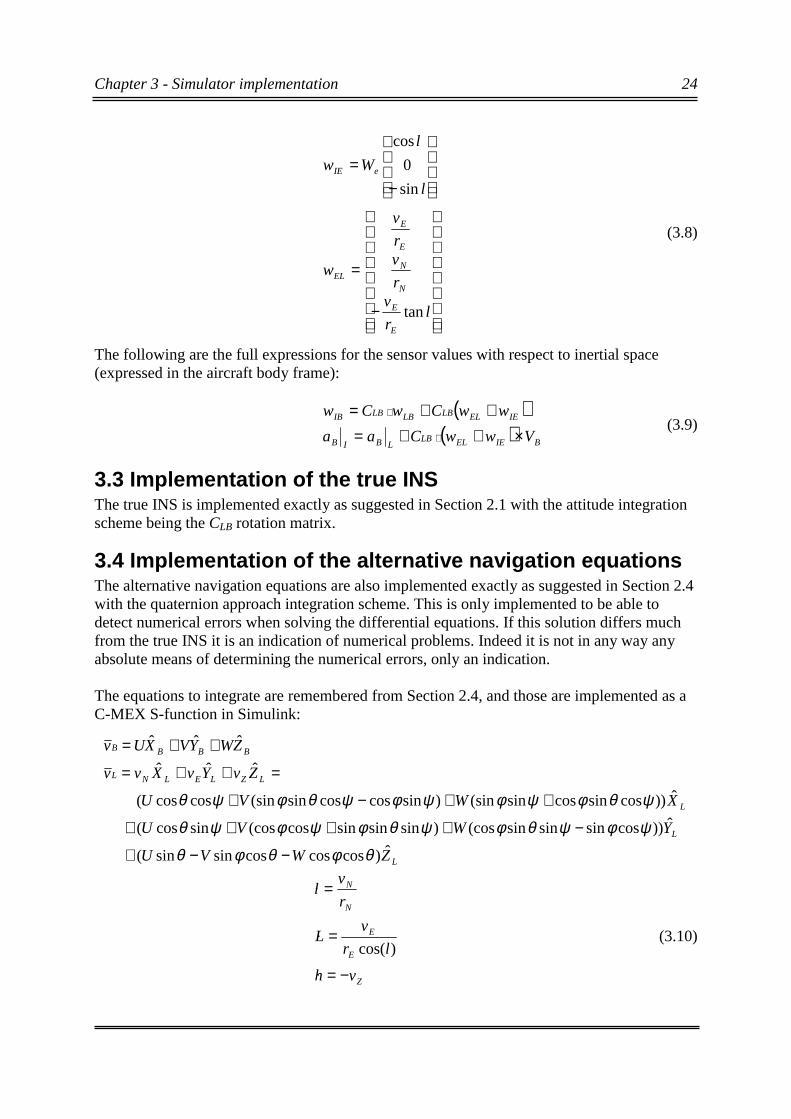
Chapter 3 - Simulator implementation 24
−
=
−=
lr
vr
vr
v
w
l
l
Ww
E
E
N
N
E
E
EL
eIE
tan
sin
0
cos
(3.8)
The following are the full expressions for the sensor values with respect to inertial space(expressed in the aircraft body frame):
( )( ) BIEELLB
LBIB
IEELLBLBLBIB
VwwCaa
wwCwCw
×++=++=
⋅
⋅(3.9)
3.3 Implementation of the true INSThe true INS is implemented exactly as suggested in Section 2.1 with the attitude integrationscheme being the CLB rotation matrix.
3.4 Implementation of the alternative navigation equationsThe alternative navigation equations are also implemented exactly as suggested in Section 2.4with the quaternion approach integration scheme. This is only implemented to be able todetect numerical errors when solving the differential equations. If this solution differs muchfrom the true INS it is an indication of numerical problems. Indeed it is not in any way anyabsolute means of determining the numerical errors, only an indication.
The equations to integrate are remembered from Section 2.4, and those are implemented as aC-MEX S-function in Simulink:
L
L
L
LZLELNL
BBBB
ZWVU
YWVU
XWVU
ZvYvXvv
ZWYVXUv
ˆ)coscoscossinsin(
ˆ))cossinsinsin(cos)sinsinsincos(cossincos(
ˆ))cossincossin(sin)sincoscossin(sincoscos(
ˆˆˆ
ˆˆˆ
θφθφθ
ψφψθφψθφψφψθ
ψθφψφψφψθφψθ
−−+
−++++
++−+
=++=
++=
Z
E
E
N
N
vh
lr
vL
r
vl
−=
=
=
�
�
�
)cos((3.10)
Chapter 3 - Simulator implementation 25
2
)(2
)(2
)(2
)(
2103
3102
3201
3210
qPqQqRq
qPqRqQq
qQqRqPq
qRqQqPq
⋅+⋅−⋅−−=
⋅−⋅+⋅−−=
⋅+⋅−⋅−−=
⋅+⋅+⋅−=
�
�
�
�
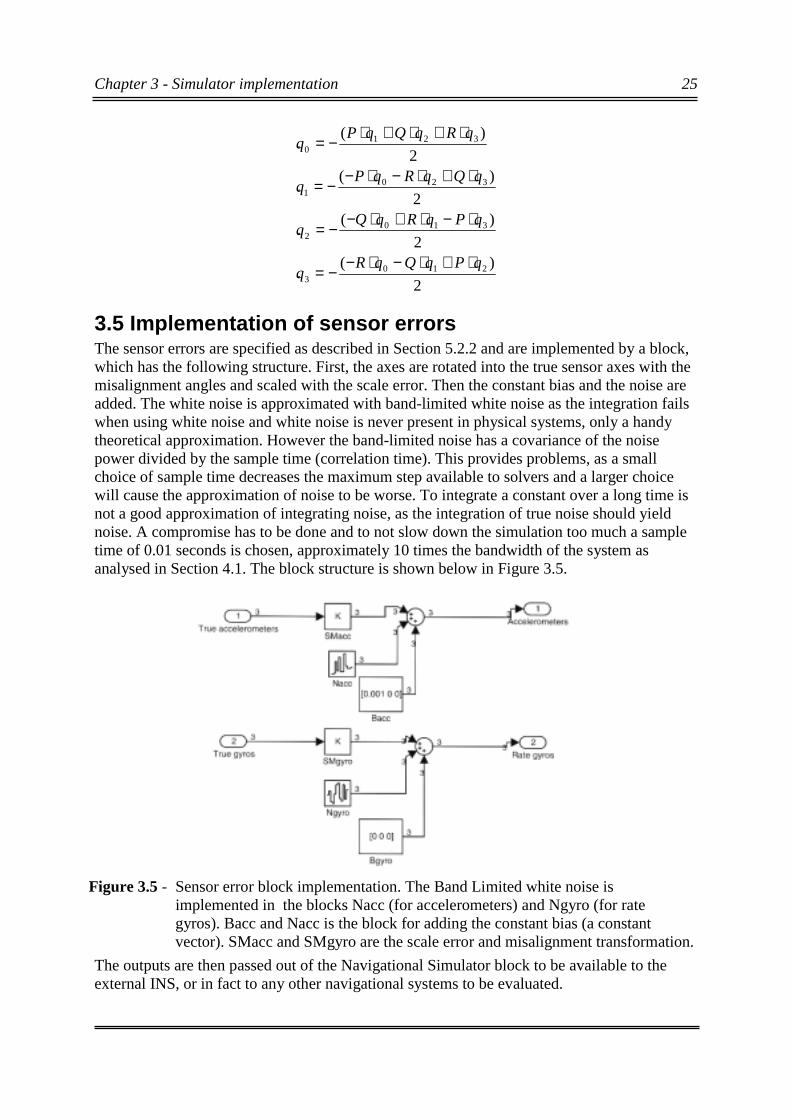
3.5 Implementation of sensor errorsThe sensor errors are specified as described in Section 5.2.2 and are implemented by a block,which has the following structure. First, the axes are rotated into the true sensor axes with themisalignment angles and scaled with the scale error. Then the constant bias and the noise areadded. The white noise is approximated with band-limited white noise as the integration failswhen using white noise and white noise is never present in physical systems, only a handytheoretical approximation. However the band-limited noise has a covariance of the noisepower divided by the sample time (correlation time). This provides problems, as a smallchoice of sample time decreases the maximum step available to solvers and a larger choicewill cause the approximation of noise to be worse. To integrate a constant over a long time isnot a good approximation of integrating noise, as the integration of true noise should yieldnoise. A compromise has to be done and to not slow down the simulation too much a sampletime of 0.01 seconds is chosen, approximately 10 times the bandwidth of the system asanalysed in Section 4.1. The block structure is shown below in Figure 3.5.
The outputs are then passed out of the Navigational Simulator block to be available to theexternal INS, or in fact to any other navigational systems to be evaluated.
Figure 3.5 - Sensor error block implementation. The Band Limited white noise is implemented in the blocks Nacc (for accelerometers) and Ngyro (for rate gyros). Bacc and Nacc is the block for adding the constant bias (a constant vector). SMacc and SMgyro are the scale error and misalignment transformation.
Chapter 3 - Simulator implementation 26
3.6 Numerical solution to the differential equationsWhen updating the simulation, the state derivatives have to be integrated. This process resultsin numerical errors, one part that comes from the calculation of the state derivatives and theother when they are actually integrated. The first part mainly consists of transformationalerrors, for instance if the condition CLB = CBL
T is not exactly true (errors mostly in the rangeof 1⋅10-16) constants transformed back and forth will not be equal. This is the case for theplumb bob gravity and the wIL rotation which is taken from the INS, transformed and thensent back. These errors, will however, cause errors that are very oscillating and even if theywere constant they would only render errors in the range of t⋅1⋅10-16 which will not be aproblem having in mind the simulation times intended. As an addition, all calculations madein MatLab or in fact on any computer system produces small numerical errors.
To solve the differential equations in the Simulink blocks, they are integrated according to asolver. There are numerous solvers available and the selection is a compromise betweenspeed, accuracy and stability. Although, in Section 4.1, we concluded the bandwidth of thesystem to be well approximated by a sample time of 0.01 seconds, this is not an adequatesample time for the solver. It is well enough to control the system but in the analysis ofinertial guidance, also small errors get integrated twice into position and results in largeerrors. Because of this problem, a variable-step solver is suggested. Rather than integrating infixed steps it decides the integration step on basis of the actual state derivatives magnitude.This improves accuracy largely since when things happen fast, integration is careful. Also itdoes not decrease much in speed as it integrates in large steps when near an equilibrium statepoint. The latter will be the case most of the time, as straight level flight is desired betweenwaypoints when the heading is corrected.
The method suggested is the Adams-Bashforth-Moulton method, a multi-step, variable-orderand variable-step method which uses the following scheme. Denote the current state by x, thestep size by h and the order by p,
∑=
−−− +=p
jjnjnjnn xtfbhxx
01 ),( (3.11)
where f is the state derivative function, ),( uxfx =� . To calculate the step size h, the solverneeds two error parameters to be specified, the relative error tolerance and the absolute errortolerance.
If the local error is larger than the accepted, the step size is halved and the process is redone.This is continued until the local error is acceptably small. This method provides a goodcompromise between accuracy and speed and is suggested for further use of this simulatingenvironment. Defining a relative error of 5e-3 and an absolute error of 2e-6, the simulationspeed on an Ultra Sparcstation 30 is 20-100% faster than real-time.
If a fast simulation is required at early development stages, a fixed-step solver with a step of0.01 seconds is suggested, it gives enough accuracy to simulate a calm flight in about 10minutes without getting too much numerical errors (in the INS). Actually such a simulation ismore than enough adequate if errors are not integrated (as in the INS).
Chapter 4 - Aircraft control 27
Chapter 4
Aircraft controlTo control the aircraft during the simulation, i.e. to get it to fly to each waypoint defining theflight path, a guidance logic system and a control surface controller is needed. Also if thecollision detection system is enabled, another guidance logic and controller is needed. Todecide what is a good enough controller an initial analysis of the system is vital, and thatincludes linearisation of the non-linear model in use.
4.1 Linearisation of the non-linear aerodynamics modelAnalysis of the non-linear system is a task where very little theoretical knowledge of suchsystems in general makes it hard. For linear systems however, control theory is welldeveloped. All of the pole-zero, Bode and other famous analysis tools, only apply to linearsystems. To be able to use these tools and make conclusions about the system a linearisationhas to be made. A single linearisation of the full non-linear system used at all states is notadequate enough. The model has to be linearised around several equilibrium points.
An equilibrium point is a point where all state derivatives are zero, which means stationaryflight, i.e. none of the state variables (velocity and rotational speeds) change. Denote thecontrol signals by u0 = [δe δa δr δt] (thrust, elevator, aileron, rudder), the statex0 = [ U, V, W, P, Q, R] and f the general non-linear function to describe the state derivatives.If
0),( 00 == uxfx� (4.1)
then the point [x0, u0] is an equilibrium point.
Let
uduu
xdxx
+=+=
0
0 (4.2)
Evaluating the differential of the non-linear function around this equilibrium point will yield alinear state space model of the form:
xCdyd
uBdxAdxd
=+=�
(4.3)
The dx and du describes the perturbation from the stationary state. As described before, asingle linearisation does not cover the full non-linear model. This implies that dx and du hasto stay small to well enough describe the true system. If the perturbation is large, the linearsystem and the non-linear will differ much and a control law developed on basis of this linearsystem will most probably be insufficient for the true system. Instead if the perturbation islarge, a new linearisation is necessary, which will result in a new controller. Indeed theoryexists to get an optimal controller based on a LQ-criteria [4]. As described later in Section 4.3this is not the approach in this master thesis, instead a simpler PID approach is chosen withthe controllers linearised in parameters instead.
Chapter 4 - Aircraft control 28
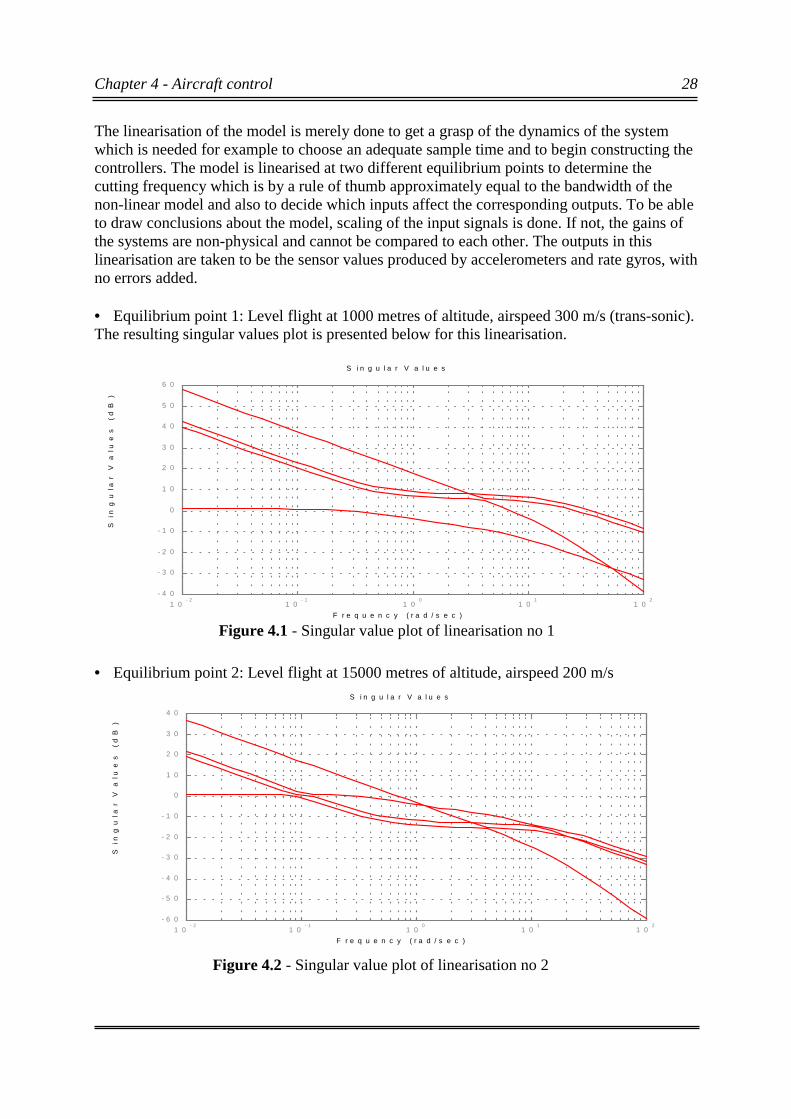
The linearisation of the model is merely done to get a grasp of the dynamics of the systemwhich is needed for example to choose an adequate sample time and to begin constructing thecontrollers. The model is linearised at two different equilibrium points to determine thecutting frequency which is by a rule of thumb approximately equal to the bandwidth of thenon-linear model and also to decide which inputs affect the corresponding outputs. To be ableto draw conclusions about the model, scaling of the input signals is done. If not, the gains ofthe systems are non-physical and cannot be compared to each other. The outputs in thislinearisation are taken to be the sensor values produced by accelerometers and rate gyros, withno errors added.
• Equilibrium point 1: Level flight at 1000 metres of altitude, airspeed 300 m/s (trans-sonic).The resulting singular values plot is presented below for this linearisation.
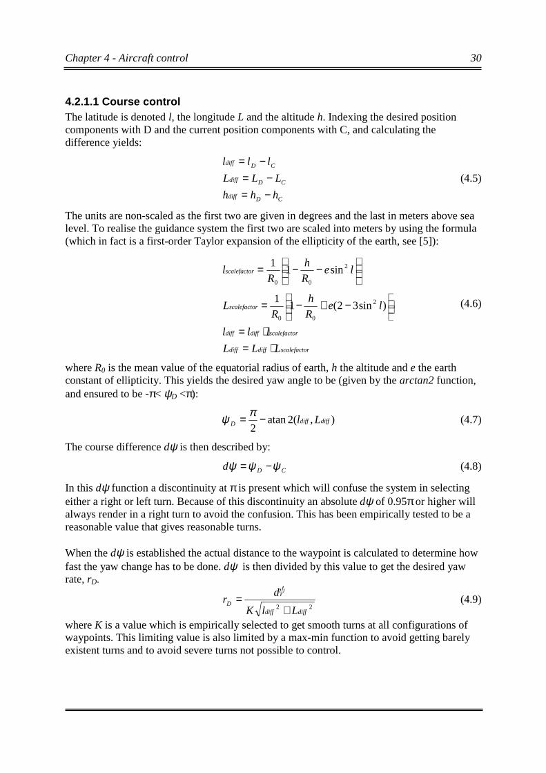
• Equilibrium point 2: Level flight at 15000 metres of altitude, airspeed 200 m/s
F r e q u e n c y ( r a d / s e c )
Sin
gu
lar
V
alu
es
(
dB
)
S i n g u l a r V a l u e s
1 0- 2
1 0- 1
1 00
1 01
1 02
- 4 0
- 3 0
- 2 0
- 1 0
0
1 0
2 0
3 0
4 0
5 0
6 0
F r e q u e n c y ( r a d / s e c )
Sin
gu
lar
V
alu
es
(
dB
)
S i n g u l a r V a l u e s
1 0- 2
1 0- 1
1 00
1 01
1 02
- 6 0
- 5 0
- 4 0
- 3 0
- 2 0
- 1 0
0
1 0
2 0
3 0
4 0
Figure 4.1 - Singular value plot of linearisation no 1
Figure 4.2 - Singular value plot of linearisation no 2

Chapter 4 - Aircraft control 29
The linearisations above imply that the cutting frequency ωc and then bandwidth ωb is wellunder 50 rad/s which by a rule of thumb given in [3] gives that the transfer function is welldescribed for frequencies under ωb if the sample time, Ts, is chosen as:
bsT
ωπ2= (4.4)
The maximum sample time to still describe the transfer functions well is then approximately0.13s and to further improve the accuracy a sample time of 0.01s is chosen (for parts of thedynamical system, the navigational equations will require more accuracy).
A conversion of the linear state space model (here at equilibrium point 1) to transfer functionsyields the following table of negligible effect on an input-output basis. A cross means input-output transfer function cannot be neglected.
Input/Output Thrust Elevator Aileron RudderAcc X X XAcc Y X XAcc Z XGyro P X XGyro Q XGyro R X X
This gives the in aerodynamics well known cross-coupling between aileron and rudder (i.e. acoordinated turn has to involve both control surfaces) but also suggests that an approach tocompletely separate the control circuits might be successful (with the exception for aileronand rudder of course).
This is the approach in control continued in Section 4.3
4.2 Guidance logicThe guidance logic is needed to produce reference signals to the controllers, to make theaircraft fly as planned (or to avoid collision if the collision avoidance system is enabled). Inone of the earlier master thesis at Saab [6] a formula for guidance of a dynamic system wassuggested. This approach is taken into consideration and developed further to be adequate forthe requirements of the waypoint guidance.
4.2.1 Waypoint guidanceThe waypoints are defined as a desired latitude, longitude, altitude and airspeed. Also aparameter called TF-logic is supplied. If TF (Terrain Follow) is on, a greater acceleration inbody z is allowed and the aircraft will with more agility get to the desired altitude. This isused when waypoints are very closely separated and on quite a straight line.
Chapter 4 - Aircraft control 30
4.2.1.1 Course controlThe latitude is denoted l, the longitude L and the altitude h. Indexing the desired positioncomponents with D and the current position components with C, and calculating thedifference yields:
CDdiff
CDdiff
CDdiff
hhh
LLL
lll
−=−=
−=(4.5)
The units are non-scaled as the first two are given in degrees and the last in meters above sealevel. To realise the guidance system the first two are scaled into meters by using the formula(which in fact is a first-order Taylor expansion of the ellipticity of the earth, see [5]):
rscalefactodiffdiff
rscalefactodiffdiff
rscalefacto
rscalefacto
LLL
lll
leR
h
RL
leR
h
Rl
⋅=⋅=
−+−=
−−=
)sin32(11
sin11
2
00
2
00
(4.6)
where R0 is the mean value of the equatorial radius of earth, h the altitude and e the earthconstant of ellipticity. This yields the desired yaw angle to be (given by the arctan2 function,and ensured to be -π< ψD <π):
),2(atan2
diffdiffD Ll−= πψ (4.7)
The course difference dψ is then described by:
CDd ψψψ −= (4.8)
In this dψ function a discontinuity at π is present which will confuse the system in selectingeither a right or left turn. Because of this discontinuity an absolute dψ of 0.95π or higher willalways render in a right turn to avoid the confusion. This has been empirically tested to be areasonable value that gives reasonable turns.
When the dψ is established the actual distance to the waypoint is calculated to determine howfast the yaw change has to be done. dψ is then divided by this value to get the desired yawrate, rD.
22diffdiff
DLlK
d¸r
+= (4.9)
where K is a value which is empirically selected to get smooth turns at all configurations ofwaypoints. This limiting value is also limited by a max-min function to avoid getting barelyexistent turns and to avoid severe turns not possible to control.
Chapter 4 - Aircraft control 31
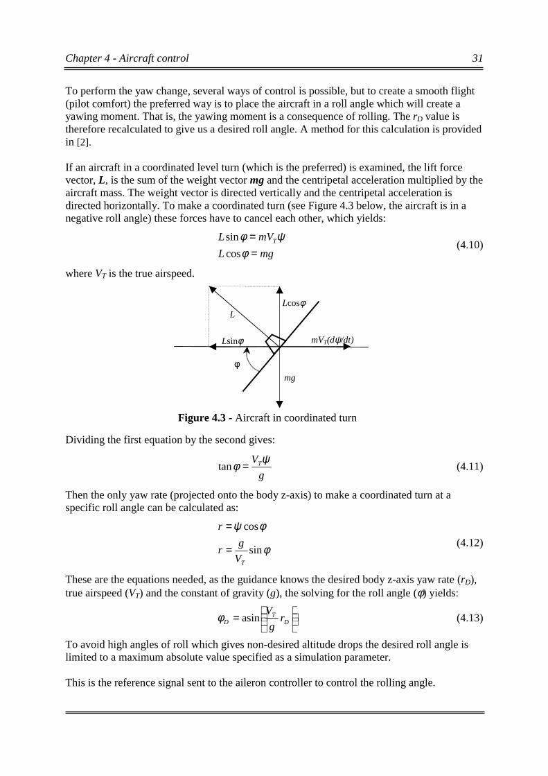
To perform the yaw change, several ways of control is possible, but to create a smooth flight(pilot comfort) the preferred way is to place the aircraft in a roll angle which will create ayawing moment. That is, the yawing moment is a consequence of rolling. The rD value istherefore recalculated to give us a desired roll angle. A method for this calculation is providedin [2].
If an aircraft in a coordinated level turn (which is the preferred) is examined, the lift forcevector, L, is the sum of the weight vector mg and the centripetal acceleration multiplied by theaircraft mass. The weight vector is directed vertically and the centripetal acceleration isdirected horizontally. To make a coordinated turn (see Figure 4.3 below, the aircraft is in anegative roll angle) these forces have to cancel each other, which yields:
mgL
mVL T
==
φψφ
cos
sin �
(4.10)
where VT is the true airspeed.
Dividing the first equation by the second gives:
g
VTψφ�
=tan (4.11)
Then the only yaw rate (projected onto the body z-axis) to make a coordinated turn at aspecific roll angle can be calculated as:
φ
φψ
sin
cos
TV
gr
r
=
= �
(4.12)
These are the equations needed, as the guidance knows the desired body z-axis yaw rate (rD),true airspeed (VT) and the constant of gravity (g), the solving for the roll angle (φ) yields:
= D
TD r
g
Vasinφ (4.13)
To avoid high angles of roll which gives non-desired altitude drops the desired roll angle islimited to a maximum absolute value specified as a simulation parameter.
This is the reference signal sent to the aileron controller to control the rolling angle.
Figure 4.3 - Aircraft in coordinated turn
φ
LLcosφ
Lsinφ
mg
mVT(dψ/dt)
Chapter 4 - Aircraft control 32
4.2.1.2 Altitude controlRemembering from Section 4.2.1.1 the calculation of the position difference,
CDdiff
CDdiff
CDdiff
hhh
LLL
lll
−=−=
−=(4.14)
and doing the same rescaling to meters is the initial step of the calculation.
The desired flightpath angle altitudewise (γD) is the arctan of the altitude difference dividedby a function of the horizontal distance to next waypoint (the K is chosen on an empiricalbasis). This value is also limited by a max-min function to avoid getting barely existent flightpath changes and to avoid severe pitch-ups not possible to control.
+=
22atan
diffdiff
diff
DLlK
hγ (4.15)
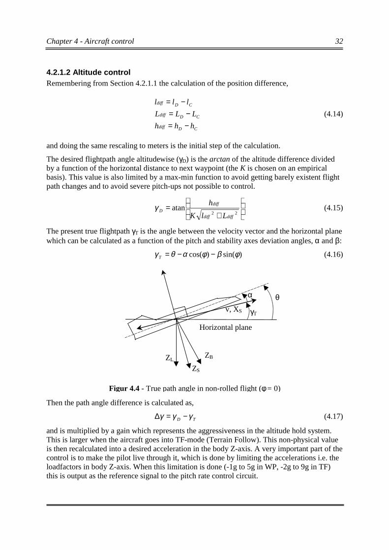
The present true flightpath γT is the angle between the velocity vector and the horizontal planewhich can be calculated as a function of the pitch and stability axes deviation angles, α and β:
)sin()cos( φβφαθγ −−=T (4.16)
Then the path angle difference is calculated as,
TD γγγ −=∆ (4.17)
and is multiplied by a gain which represents the aggressiveness in the altitude hold system.This is larger when the aircraft goes into TF-mode (Terrain Follow). This non-physical valueis then recalculated into a desired acceleration in the body Z-axis. A very important part of thecontrol is to make the pilot live through it, which is done by limiting the accelerations i.e. theloadfactors in body Z-axis. When this limitation is done (-1g to 5g in WP, -2g to 9g in TF)this is output as the reference signal to the pitch rate control circuit.
ZS
Figur 4.4 - True path angle in non-rolled flight (φ = 0)
v, XS
α
Horizontal plane
ZBZL
γT
θ
Chapter 4 - Aircraft control 33
4.2.2 Collision avoidance guidanceThe guidance for collision avoidance is not an objective of this thesis, but is presently beingexamined in another master thesis at Saab. Because of this need for a simulator environment,the possibility is included in the simulator, but only for ground collision. In the other thesismid-air collisions is the main part.
The guidance is fairly simple. When the n-second (n is a GCAS specified parameter) aheadpredicted altitude goes below a specified value the (Ground) Collision Avoidance System(CAS) takes control. A loadfactor vector directed up from the ground (local frame Z-axis) istransformed into body coordinates with the present attitude to form the reference loadfactor.This is then sent to the loadfactor controller circuit to produce the desired avoidance.
This guidance is not in any way optimal and will at some attitudes actually worsen orunstabilise the situation, but this goes beyond the scope of this thesis.

Chapter 4 - Aircraft control 34
4.3 Control in Waypoint navigation modeThe control objectives in waypoint navigation mode are primarily to get the aircraft to get tofollow the reference signals with high pilot comfort i.e. the accelerations experienced by thepilot should be small. Also a clean state of flight is desired in pilot comfort, which means thatthe velocity component in body y-axis should be kept small i.e. small beta angles. Assuggested in Section 4.1 only a low degree of cross-coupling between the control circuits ispresent, except for the aileron and rudder circuits. The approach is to separate the probleminto four independent controllers. Furthermore, the basic approach of PID-control is applied.The controllers below are non-linear but will be called PID-controllers anyway.
4.3.1 Thrust controlReference signals: Desired airspeed, desired acceleration in body x-axis.Measurement signals: Airspeed, acceleration in body x-axis (i.e. loadfactor), measured
dragOutput signal: A desired thrust power to be actuated by the engine.
The thrust control circuit will be discussed in detail, to introduce the reader how to interpretthe Simulink diagrams. The rest of the control circuits will then be left to the reader tointerpret. The thrust control circuit is a P-controller as in Figure 4.5 below:
At the top left the difference between the airspeed of the aircraft and the desired airspeed iscalculated and then multiplied by the gain to form the part, which pushes the engine toproduce force to obtain the desired airspeed. This part is also saturated to avoid severe thrustjumps when passing a waypoint, where desired airspeed might change. The difference will,performed in this way, be vanishing smoothly.
The second part is where a desired acceleration the body x-axis is multiplied by the mass toobtain the needed force to get this acceleration. It is saturated of the same reason as statedabove.
The last part is a drag force measurement, which actually measures the true drag forceproduced by the airflow, which is for now taken directly from the model. To get a morerealistic approach, this could be replaced by a more realistic model of the measurement.
1
T hrust
S um to t
S um
S atu ra tio nT hrust
S a tu ra tio nS PE ED
S atu ra tio nA CCP ro duct
-1
G a in1
20 00
G a in
[M ass]
4
M ea su red a i r resi sta nce
3
Desi red a i rspe ed
2
T ru e a i rsp eed
1
Desi red a cce la ra ti on (bod y X )
Figure 4.5 - Thrust control circuit

Chapter 4 - Aircraft control 35
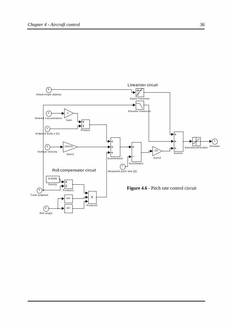
4.3.2 Pitch controlReference signals: Desired acceleration in body z-axis.Measurement signals: Vertical velocity, pitch rate, airspeed, attack angle, roll angleOutput signal: A desired deflection of the elevator control surface.
The pitch rate controller is more complicated (but in principle only a kind of PD-controller),first the reference is calculated into a desired pitch rate qdes considering the formula (signchange due to z-axis pointing down):
U
ahzqdes −= (4.18)
where ahz is the desired acceleration in body z-axis and U is the velocity component in bodyx-axis.
A damping factor (corresponding to a D-part in a PID) is introduced to avoid too much climbor descent. It also helps stabilising the altitude when the correct altitude is reached. Thedamping factor is a gain of the vertical velocity (local frame z-axis)
A major problem of pitch control is that the pitching moment's equilibrium differsenormously with airspeed. To keep track of this equilibrium, a linearisation circuit isintroduced. The circuit is a table of equilibrium values against airspeed, and the output is aninterpolation of two points in the table. The table is setup by performing experiments with thefull non-linear model. When getting close to transonic speeds (which is modelled) theequilibrium value is very unstable and the points have to be sampled closer in the table. Thisproblem is not solved fully, getting close to transonic speeds may at some attitudes renderclosed loop instability which causes the aircraft to crash. To improve the linearisation, asimilar table of attack angle dependence is also used.
Also when rolling the aircraft loses lift power in reference to gravity which will cause theaircraft to make an undesired altitude drop. To compensate for this an approach to lift thenose as the aircraft goes into a roll is implemented. The following formula applies [2]:
)sin()tan( φφT
D V
gq = (4.19)
This only works when the rolling angles are small enough, at for instance 90 degrees of rollthe pitching up actually does not work at all in the aim of altitude hold. The desired pitch rateis calculated by summing up the part expressions.
The full elevator control circuit is shown in Figure 4.6 below:
Chapter 4 - Aircraft control 36
Roll compensator circuit
Linearizer circuit
1
Elevator
sin
tan
Sumtot
SumDesired
SumDesacc
SaturationElevator
Product2
Product1
Product
9.8066
Gravi ty
-25
Gain2
.00015
Gain1
-1
Gain
Elevator l inearizer
Alpha l inearizer
7
Measured pi tch rate (Q)
6
Attack Angle (alpha)
5
T otal ai rspeed
4
Rol l angle
3
Vertical veloci ty
2
Desired z-acceleration
1
Airspeed body x (U)
Figure 4.6 - Pitch rate control circuit
Chapter 4 - Aircraft control 37
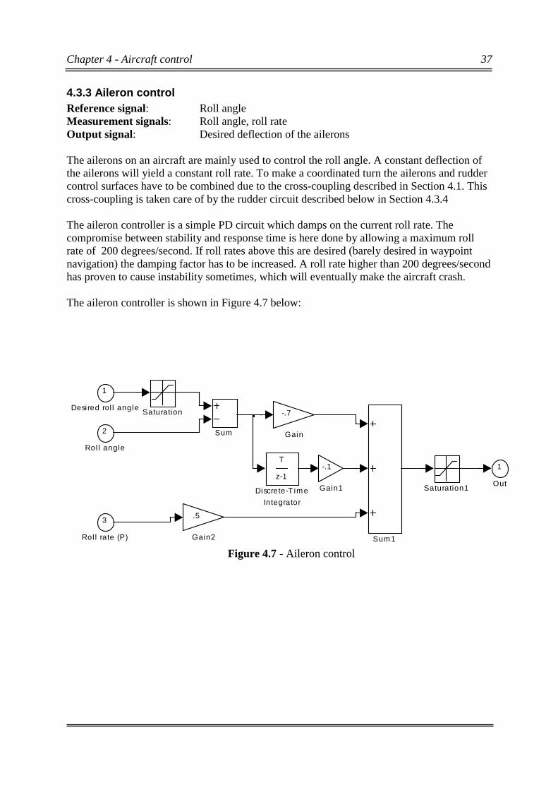
4.3.3 Aileron controlReference signal: Roll angleMeasurement signals: Roll angle, roll rateOutput signal: Desired deflection of the ailerons
The ailerons on an aircraft are mainly used to control the roll angle. A constant deflection ofthe ailerons will yield a constant roll rate. To make a coordinated turn the ailerons and ruddercontrol surfaces have to be combined due to the cross-coupling described in Section 4.1. Thiscross-coupling is taken care of by the rudder circuit described below in Section 4.3.4
The aileron controller is a simple PD circuit which damps on the current roll rate. Thecompromise between stability and response time is here done by allowing a maximum rollrate of 200 degrees/second. If roll rates above this are desired (barely desired in waypointnavigation) the damping factor has to be increased. A roll rate higher than 200 degrees/secondhas proven to cause instability sometimes, which will eventually make the aircraft crash.
The aileron controller is shown in Figure 4.7 below:
1
Out
Sum1
Sum
Saturation1
Saturation
.5
Gain2
-.1
Gain1
-.7
Gain
T
z-1
Discrete-T ime
Integrator
3
Rol l rate (P)
2
Rol l angle
1
Desired rol l angle
Figure 4.7 - Aileron control
Chapter 4 - Aircraft control 38
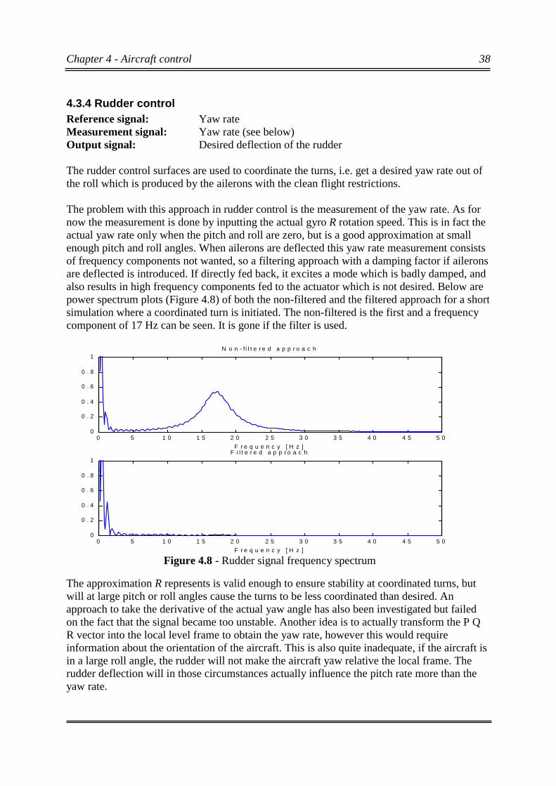
4.3.4 Rudder controlReference signal: Yaw rateMeasurement signal: Yaw rate (see below)Output signal: Desired deflection of the rudder
The rudder control surfaces are used to coordinate the turns, i.e. get a desired yaw rate out ofthe roll which is produced by the ailerons with the clean flight restrictions.
The problem with this approach in rudder control is the measurement of the yaw rate. As fornow the measurement is done by inputting the actual gyro R rotation speed. This is in fact theactual yaw rate only when the pitch and roll are zero, but is a good approximation at smallenough pitch and roll angles. When ailerons are deflected this yaw rate measurement consistsof frequency components not wanted, so a filtering approach with a damping factor if aileronsare deflected is introduced. If directly fed back, it excites a mode which is badly damped, andalso results in high frequency components fed to the actuator which is not desired. Below arepower spectrum plots (Figure 4.8) of both the non-filtered and the filtered approach for a shortsimulation where a coordinated turn is initiated. The non-filtered is the first and a frequencycomponent of 17 Hz can be seen. It is gone if the filter is used.
The approximation R represents is valid enough to ensure stability at coordinated turns, butwill at large pitch or roll angles cause the turns to be less coordinated than desired. Anapproach to take the derivative of the actual yaw angle has also been investigated but failedon the fact that the signal became too unstable. Another idea is to actually transform the P QR vector into the local level frame to obtain the yaw rate, however this would requireinformation about the orientation of the aircraft. This is also quite inadequate, if the aircraft isin a large roll angle, the rudder will not make the aircraft yaw relative the local frame. Therudder deflection will in those circumstances actually influence the pitch rate more than theyaw rate.
0 5 1 0 1 5 2 0 2 5 3 0 3 5 4 0 4 5 5 00
0 . 2
0 . 4
0 . 6
0 . 8
1N o n - f i l t e r e d a p p r o a c h
F r e q u e n c y [ H z ]
0 5 1 0 1 5 2 0 2 5 3 0 3 5 4 0 4 5 5 00
0 . 2
0 . 4
0 . 6
0 . 8
1
F r e q u e n c y [ H z ]
F i l t e r e d a p p r o a c h
Figure 4.8 - Rudder signal frequency spectrum
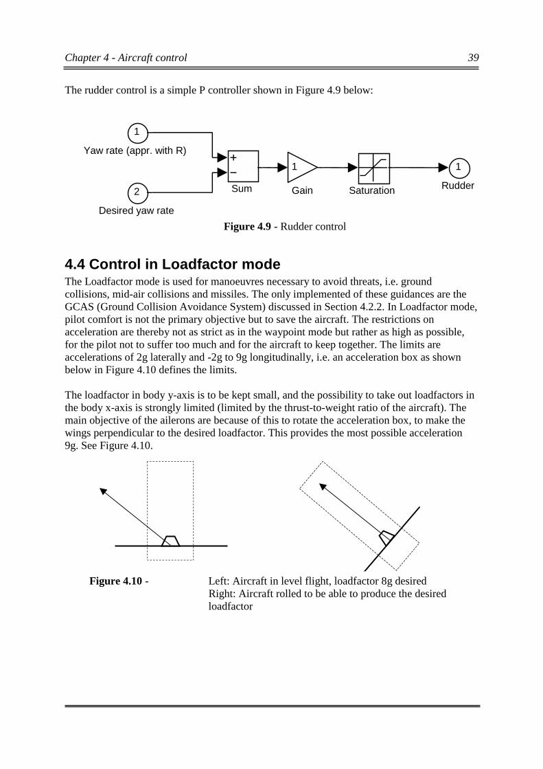
Chapter 4 - Aircraft control 39
The rudder control is a simple P controller shown in Figure 4.9 below:
4.4 Control in Loadfactor modeThe Loadfactor mode is used for manoeuvres necessary to avoid threats, i.e. groundcollisions, mid-air collisions and missiles. The only implemented of these guidances are theGCAS (Ground Collision Avoidance System) discussed in Section 4.2.2. In Loadfactor mode,pilot comfort is not the primary objective but to save the aircraft. The restrictions onacceleration are thereby not as strict as in the waypoint mode but rather as high as possible,for the pilot not to suffer too much and for the aircraft to keep together. The limits areaccelerations of 2g laterally and -2g to 9g longitudinally, i.e. an acceleration box as shownbelow in Figure 4.10 defines the limits.
The loadfactor in body y-axis is to be kept small, and the possibility to take out loadfactors inthe body x-axis is strongly limited (limited by the thrust-to-weight ratio of the aircraft). Themain objective of the ailerons are because of this to rotate the acceleration box, to make thewings perpendicular to the desired loadfactor. This provides the most possible acceleration9g. See Figure 4.10.
1
RudderSum Saturation
1
Gain2
Desired yaw rate
1
Yaw rate (appr. with R)
Figure 4.9 - Rudder control
Figure 4.10 - Left: Aircraft in level flight, loadfactor 8g desiredRight: Aircraft rolled to be able to produce the desiredloadfactor
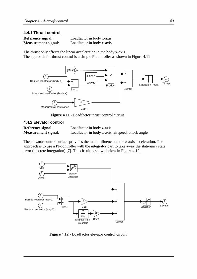
Chapter 4 - Aircraft control 40
4.4.1 Thrust controlReference signal: Loadfactor in body x-axisMeasurement signal: Loadfactor in body x-axis
The thrust only affects the linear acceleration in the body x-axis.The approach for thrust control is a simple P-controller as shown in Figure 4.11
4.4.2 Elevator controlReference signal: Loadfactor in body z-axisMeasurement signal: Loadfactor in body z-axis, airspeed, attack angle
The elevator control surface provides the main influence on the z-axis acceleration. Theapproach is to use a PI-controller with the integrator part to take away the stationary stateerror (discrete integration) [7]. The circuit is shown below in Figure 4.12.
Figure 4.11 - Loadfactor thrust control circuit
Figure 4.12 - Loadfactor elevator control circuit
1
Thrust
SumtotSum1
SaturationThrustProduct
9.8066
Gravity
-1
Gain
[Mass]
3
Measured loadfactor (body X)
2
Measured air resistance
1
Desired loadfactor (body X)
1
Elevator
Sumtot
Sum1 Saturation
-.01
Gain1
-.5
Gain
ElevatorLineariser
T
z-1
Discrete-TimeIntegrator
4
Desired loadfactor (body Z)
3
Alpha
2
Measured loadfactor (body Z)
1
Vtot
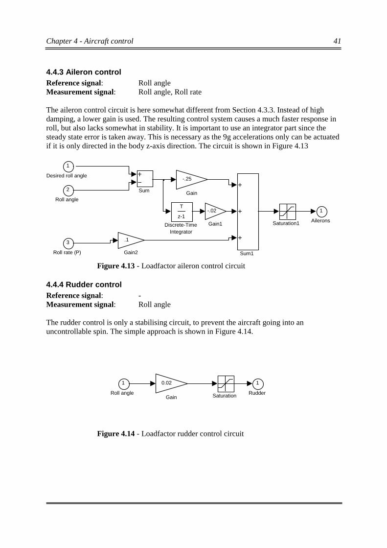
Chapter 4 - Aircraft control 41
4.4.3 Aileron controlReference signal: Roll angleMeasurement signal: Roll angle, Roll rate
The aileron control circuit is here somewhat different from Section 4.3.3. Instead of highdamping, a lower gain is used. The resulting control system causes a much faster response inroll, but also lacks somewhat in stability. It is important to use an integrator part since thesteady state error is taken away. This is necessary as the 9g accelerations only can be actuatedif it is only directed in the body z-axis direction. The circuit is shown in Figure 4.13
4.4.4 Rudder controlReference signal: -Measurement signal: Roll angle
The rudder control is only a stabilising circuit, to prevent the aircraft going into anuncontrollable spin. The simple approach is shown in Figure 4.14.
Figure 4.13 - Loadfactor aileron control circuit
Figure 4.14 - Loadfactor rudder control circuit
1
RudderSaturation
0.02
Gain
1
Roll angle
1
Ailerons
Sum1
Sum
Saturation1
.1
Gain2
-.02
Gain1
-.25
Gain
T
z-1
Discrete-TimeIntegrator
3
Roll rate (P)
2
Roll angle
1
Desired roll angle
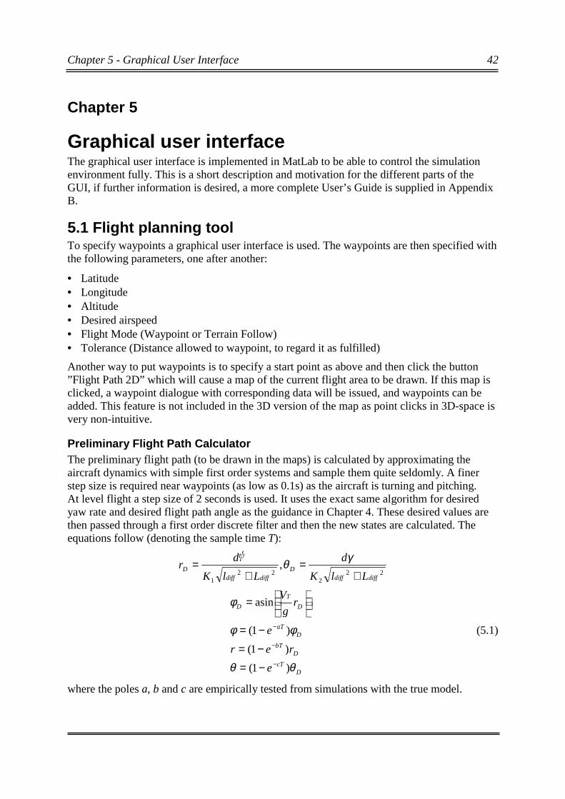
Chapter 5 - Graphical User Interface 42
Chapter 5
Graphical user interfaceThe graphical user interface is implemented in MatLab to be able to control the simulationenvironment fully. This is a short description and motivation for the different parts of theGUI, if further information is desired, a more complete User’s Guide is supplied in AppendixB.
5.1 Flight planning toolTo specify waypoints a graphical user interface is used. The waypoints are then specified withthe following parameters, one after another:
• Latitude• Longitude• Altitude• Desired airspeed• Flight Mode (Waypoint or Terrain Follow)• Tolerance (Distance allowed to waypoint, to regard it as fulfilled)
Another way to put waypoints is to specify a start point as above and then click the button”Flight Path 2D” which will cause a map of the current flight area to be drawn. If this map isclicked, a waypoint dialogue with corresponding data will be issued, and waypoints can beadded. This feature is not included in the 3D version of the map as point clicks in 3D-space isvery non-intuitive.
Preliminary Flight Path CalculatorThe preliminary flight path (to be drawn in the maps) is calculated by approximating theaircraft dynamics with simple first order systems and sample them quite seldomly. A finerstep size is required near waypoints (as low as 0.1s) as the aircraft is turning and pitching.At level flight a step size of 2 seconds is used. It uses the exact same algorithm for desiredyaw rate and desired flight path angle as the guidance in Chapter 4. These desired values arethen passed through a first order discrete filter and then the new states are calculated. Theequations follow (denoting the sample time T):
222
221
,diffdiff
Ddiffdiff
DLlK
d
LlK
d¸r
+=
+= γθ
DcT
DbT
DaT
D
T
D
e
rer
e
rg
V
θθ
φφ
φ
)1(
)1(
)1(
asin
−
−
−
−=
−=
−=
=
(5.1)
where the poles a, b and c are empirically tested from simulations with the true model.
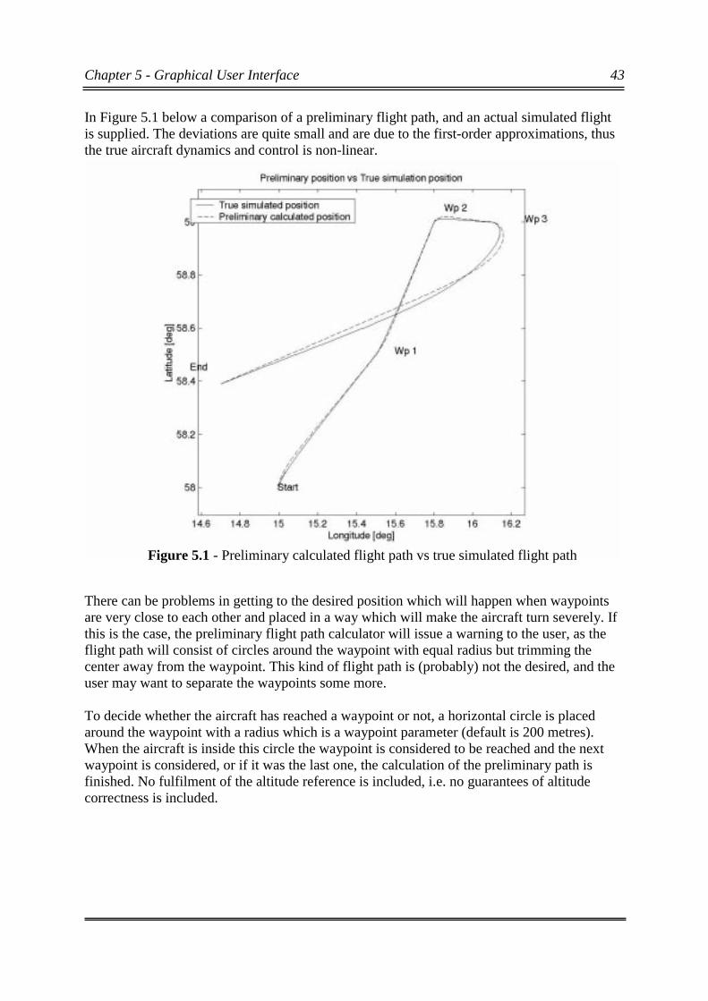
Chapter 5 - Graphical User Interface 43
In Figure 5.1 below a comparison of a preliminary flight path, and an actual simulated flightis supplied. The deviations are quite small and are due to the first-order approximations, thusthe true aircraft dynamics and control is non-linear.
There can be problems in getting to the desired position which will happen when waypointsare very close to each other and placed in a way which will make the aircraft turn severely. Ifthis is the case, the preliminary flight path calculator will issue a warning to the user, as theflight path will consist of circles around the waypoint with equal radius but trimming thecenter away from the waypoint. This kind of flight path is (probably) not the desired, and theuser may want to separate the waypoints some more.
To decide whether the aircraft has reached a waypoint or not, a horizontal circle is placedaround the waypoint with a radius which is a waypoint parameter (default is 200 metres).When the aircraft is inside this circle the waypoint is considered to be reached and the nextwaypoint is considered, or if it was the last one, the calculation of the preliminary path isfinished. No fulfilment of the altitude reference is included, i.e. no guarantees of altitudecorrectness is included.
Figure 5.1 - Preliminary calculated flight path vs true simulated flight path
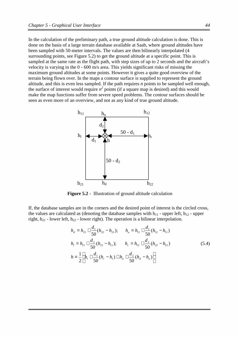
Chapter 5 - Graphical User Interface 44
In the calculation of the preliminary path, a true ground altitude calculation is done. This isdone on the basis of a large terrain database available at Saab, where ground altitudes havebeen sampled with 50-meter intervals. The values are then bilinearly interpolated (4surrounding points, see Figure 5.2) to get the ground altitude at a specific point. This issampled at the same rate as the flight path, with step sizes of up to 2 seconds and the aircraft’svelocity is varying in the 0 - 600 m/s area. This yields significant risks of missing themaximum ground altitudes at some points. However it gives a quite good overview of theterrain being flown over. In the maps a contour surface is supplied to represent the groundaltitude, and this is even less sampled. If the path requires n points to be sampled well enough,the surface of interest would require n2 points (if a square map is desired) and this wouldmake the map functions suffer from severe speed problems. The contour surfaces should beseen as even more of an overview, and not as any kind of true ground altitude.
If, the database samples are in the corners and the desired point of interest is the circled cross,the values are calculated as (denoting the database samples with h11 - upper left, h12 - upperright, h21 - lower left, h22 - lower right). The operation is a bilinear interpolation.
−++−+=
−+=−+=
−+=−+=
)(50
)(502
1
)(50
);(50
)(50
);(50
21
12222
1211212
11
11121
1121221
21
udulrl
rl
ud
hhd
hhhd
hh
hhd
hhhhd
hh
hhd
hhhhd
hh
(5.4)
50 - d1
50 - d2
d2
d1
h11 h12
h21 h22hd
hu
hrhlh
Figure 5.2 - Illustration of ground altitude calculation
Chapter 5 - Graphical User Interface 45
Flight Path VisualiserThere are two functions for flight path visualisation, one 2-dimensional and one 3-dimensional. Both use the same algorithm to calculate the flightpath, as described above. In 2-D the ground altitude is represented by a contour plot and in 3-D it is represented by a surfacerendered with light shading. The 2-D plot may also be selected to show the type of terrain bycolour coding the terrain types. This is done with the same resolution as the terrain altitude.
The waypoints are marked and the calculated preliminary vehicle path is presented. Also afew landmarks are presented, mainly cities.
The 2-dimensional plot also includes an altitude vs ground height plot to see how close to theterrain the flight will be. If ground is preliminary hit, i.e. aircraft is in danger of crashing, awarning marker will be placed at that point in time.
To insert a new waypoint, the user only has to click on the map and a dialogue will appearwith position values already inserted. After accepting, the GUI will ask the user if thepreliminary path is to be updated with the new waypoint or not. There is also possibilities tozoom and scroll on the map. A right-click on the map will show a dialogue box with theground altitude and type of terrain at the point clicked.
A visualisation of an example flightpath is shown below in Figure 5.3.
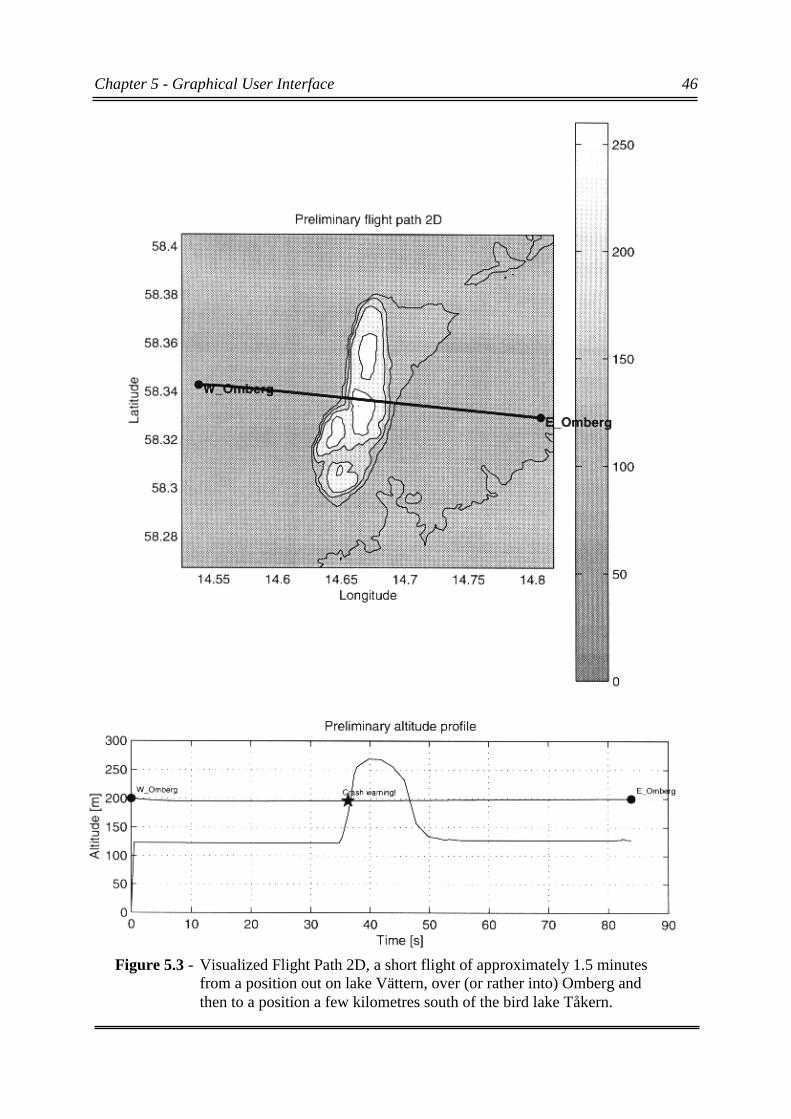
Chapter 5 - Graphical User Interface 46
Figure 5.3 - Visualized Flight Path 2D, a short flight of approximately 1.5 minutesfrom a position out on lake Vättern, over (or rather into) Omberg andthen to a position a few kilometres south of the bird lake Tåkern.
Chapter 5 - Graphical User Interface 47
5.2 Other parts of the GUIBelow are descriptions of all parts of the GUI, needed to preliminary setup a simulation.When all steps are finished, the simulation can be initialised with a single button-click.
5.2.1 Initial stateHere the initial velocity (measured in body frame), the initial attitude and initial rotations arespecified. This is required both to be able to initialise the simulation, but also to be able tocalculate a correct preliminary flight path.
5.2.2 Sensor ErrorsAll the sensor errors are input here and they are input as a mean value and a standarddeviation, this will then be randomised at every simulator initialisation. If a deterministicvalue is required (default), input zero as the standard deviation. The randomiser uses a normaldistribution. The sensor errors are (for both accelerometers and gyroscopes): bias, scale factorerror, misalignment and noise. The noise is entered as a standard deviation, σ.
5.2.3 Simulation ParametersThe top model name has to be specified, i.e. where the ”Navigation Simulator” block isplaced. Also the name of the block can be specified, if the default ”Navigation Simulator” isnot wanted. Optionally an external INS can be named, which also has to reside on the toplevel of the Simulink model. Doing this will automatically initialise it on simulatorinitialisation, this also yields the necessity of the block specified taking the exact sameparameters as the developed INS-block. If an INS is specified, initial system errors in the INScan also be specified in another dialogue.
Subsystems can be chosen to be enabled/disabled. The subsystems are GCAS, NumericalSupervisor, Ground Detection, Instrument panel displays and also if external estimates is tobe used by the control system, such an input port can be selected to appear here. If externalestimates are to be used they must be connected or the simulation will fail.
The Workspace Output variables selected, will be sampled at a rate specified in the DataAcquisition section here. Different sample rates for the aerodynamical and navigational datacan be selected.
Chapter 5 - Graphical User Interface 48
5.2.4 Workspace OutputIn this part, the selection of variables to go out to the workspace is performed. The variablesare selected from those available in two different sections, aerodynamical and navigationaldata. The following variables can be output to workspace:
Aerodynamical data Navigational data (True)Attack angle LatitudeSideslip angle LongitudeLoadfactor (body X) AltitudeLoadfactor (body Y) Velocity (local X, North)Loadfactor (body Z) Velocity (local Y, East)U- Velocity (body X) Velocity (local Z, Down)V- Velocity (body Y) Yaw angle (heading)W- Velocity (body Z) Roll angleP - Roll rotation Pitch angleQ - Pitch rotation Ground altitude*R - Yaw rotationThrustElevator deflectionAileron deflectionRudder deflection* Only available if GDS (Ground Detection System) is on, this will be a zero-vectorotherwise.
5.3 Evaluation ToolThis interface is for evaluating errors and requires the simulation to include the availableblock ”EvalExportVars” on the top level. It also requires the navigational workspace output tobe in default mode, i.e. no removal or reordering of the variables may be done. If so, theevaluation interface will produce unpredicted results.
This GUI lets the user plot different datas acquired during the simulation, for performingevaluation of errors in the estimates produced. Position, attitude and velocities are theestimated variables of interest and can be plotted independently, true or estimated, or aserrors. The Evaluation Tool is furtherly discussed in the User’s Guide in appendix B.
Chapter 6 - Simulator validation 49
Chapter 6
6 Simulator validationThis chapter is dedicated to simulator validation, to prove the validity of simulated results.This is done with respect to numerical stability but most importantly with respect to thenavigational validity. The latter is the more important as this is the main objective of thethesis, to simulate navigational algorithms.
6.1 Numerical stability examinationUnfortunately no computer-based solver is perfect and numerical errors always comes intoplay. The magnitude of the errors are dependent on things like how fast does the derivativeschange, how often do they change and also of course the total time in flight. An exactexpression for these errors is very hard to develop, if not impossible. The simulatorenvironment instead uses two approaches at solving the equations, as remembered fromChapter 2, both a true INS and an internal value based quaternion approach. When these twosolutions start to differ, it implies a numerical error. There are two main sources of numericalerrors, transformational errors and integration errors.
6.1.1 Steady level flightThe first case to be examined is a 5000 second steady state level flight, no attitude changestake place (except when stabilising in the very beginning). The difference between the twosolutions is presented below in Figure 6.1 and 6.2.
6.1.2 Non-steady, non-level flightThe second case to be examined is another 5000 second flight but with very much of attitudechanges, the aircraft lies in coordinated turns most of the time in the air. Also altitude changesare part of the flightpath which causes the aircraft to pitch severely. Again, the differencebetween the two solutions is presented below in Figure 6.3 and 6.4.
The conclusions made from these plots are that the solver is more than adequate for the twokinds of simulations. Errors in the first case stay small, and consists mostly of initialnumerical initialisation errors. The second case is interesting, almost all manoeuvres takingplace in Waypoint mode is made by rolling out to correct the heading and then roll back tolevel flight. This makes the aircraft roll in both directions and as seen by the plots, theresulting errors are in most cases very forgiving, i.e. a roll back reduces the error from rollingout. However, position and altitude suffers from growing errors which would be a problem ifa flight of very long time were desired. This is not the case for this simulator, and thenumerical errors are because of this, in these cases acceptable.
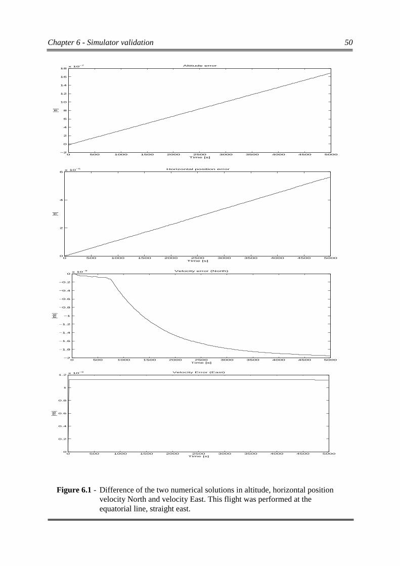
Chapter 6 - Simulator validation 50
Figure 6.1 - Difference of the two numerical solutions in altitude, horizontal positionvelocity North and velocity East. This flight was performed at theequatorial line, straight east.
0 500 1000 1500 2000 2500 3000 3500 4000 4500 5000−2
0
2
4
6
8
10
12
14
16
18x 10
−7 Altitude error
Time [s]
[m]
0 500 1000 1500 2000 2500 3000 3500 4000 4500 50000
2
4
6x 10
−5 Horizontal position error
Time [s]
[m]
0 500 1000 1500 2000 2500 3000 3500 4000 4500 5000−2
−1.8
−1.6
−1.4
−1.2
−1
−0.8
−0.6
−0.4
−0.2
0x 10
−9 Velocity error (North)
Time [s]
[m/s]
0 500 1000 1500 2000 2500 3000 3500 4000 4500 50000
0.2
0.4
0.6
0.8
1
1.2x 10
−8 Velocity Error (East)
Time [s]
[m/s]
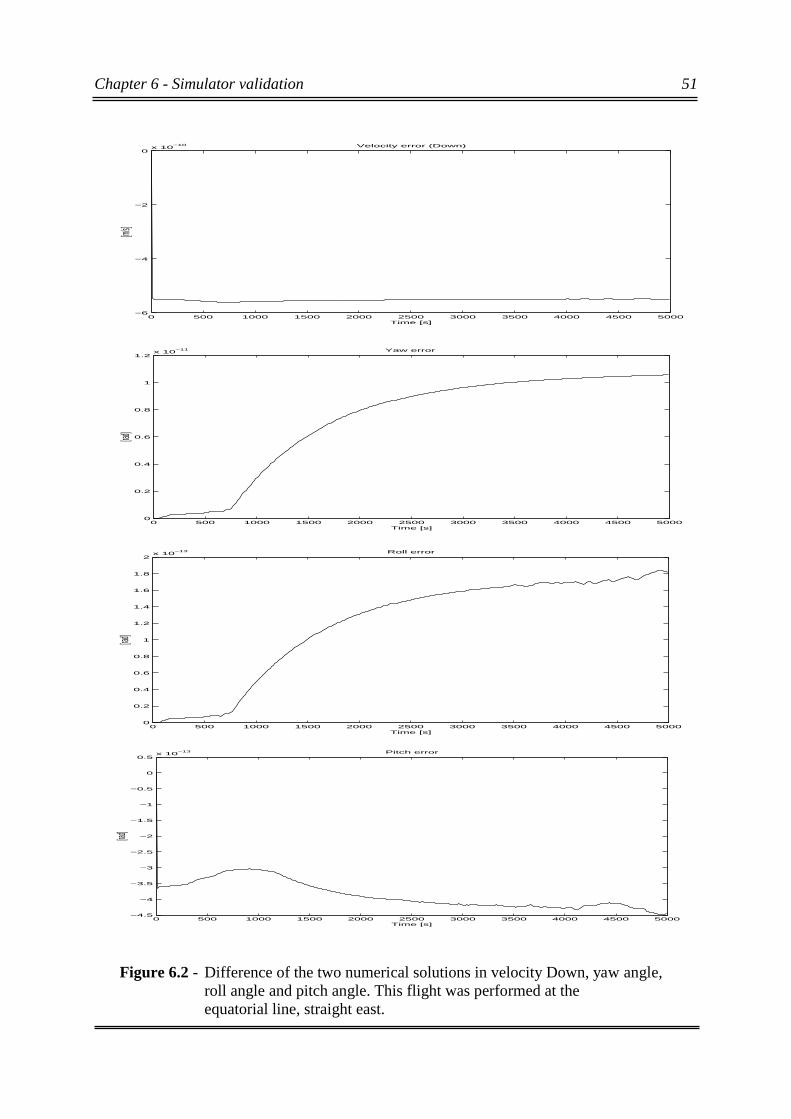
Chapter 6 - Simulator validation 51
Figure 6.2 - Difference of the two numerical solutions in velocity Down, yaw angle,roll angle and pitch angle. This flight was performed at theequatorial line, straight east.
0 500 1000 1500 2000 2500 3000 3500 4000 4500 5000−6
−4
−2
0x 10
−10 Velocity error (Down)
Time [s]
[m/s]
0 500 1000 1500 2000 2500 3000 3500 4000 4500 50000
0.2
0.4
0.6
0.8
1
1.2x 10
−11 Yaw error
Time [s]
[rad]
0 500 1000 1500 2000 2500 3000 3500 4000 4500 50000
0.2
0.4
0.6
0.8
1
1.2
1.4
1.6
1.8
2x 10
−13 Roll error
Time [s]
[rad]
0 500 1000 1500 2000 2500 3000 3500 4000 4500 5000−4.5
−4
−3.5
−3
−2.5
−2
−1.5
−1
−0.5
0
0.5x 10
−13 Pitch error
Time [s]
[rad]
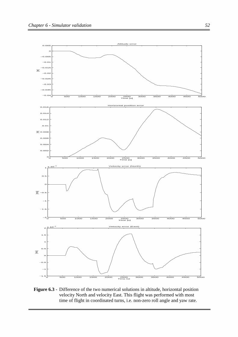
Chapter 6 - Simulator validation 52
Figure 6.3 - Difference of the two numerical solutions in altitude, horizontal positionvelocity North and velocity East. This flight was performed with mosttime of flight in coordinated turns, i.e. non-zero roll angle and yaw rate.
0 500 1000 1500 2000 2500 3000 3500 4000 4500 5000−0.04
−0.035
−0.03
−0.025
−0.02
−0.015
−0.01
−0.005
0
0.005Altitude error
Time [s]
[m]
0 500 1000 1500 2000 2500 3000 3500 4000 4500 50000
0.002
0.004
0.006
0.008
0.01
0.012
0.014
0.016Horizontal position error
Time [s]
[m]
0 500 1000 1500 2000 2500 3000 3500 4000 4500 5000−2
−1.5
−1
−0.5
0
0.5
1x 10
−5 Velocity error (North)
Time [s]
[m/s]
0 500 1000 1500 2000 2500 3000 3500 4000 4500 5000−1.5
−1
−0.5
0
0.5
1
1.5
2x 10
−5 Velocity error (East)
Time [s]
[m/s]
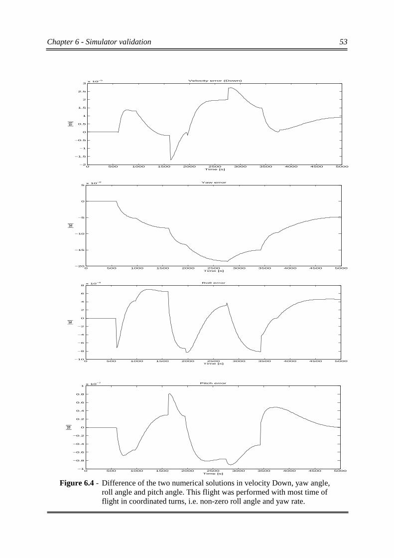
Chapter 6 - Simulator validation 53
Figure 6.4 - Difference of the two numerical solutions in velocity Down, yaw angle,roll angle and pitch angle. This flight was performed with most time offlight in coordinated turns, i.e. non-zero roll angle and yaw rate.
0 500 1000 1500 2000 2500 3000 3500 4000 4500 5000−2
−1.5
−1
−0.5
0
0.5
1
1.5
2
2.5
3x 10
−5 Velocity error (Down)
Time [s]
[m/s]
0 500 1000 1500 2000 2500 3000 3500 4000 4500 5000−20
−15
−10
−5
0
5x 10
−8 Yaw error
Time [s]
[rad]
0 500 1000 1500 2000 2500 3000 3500 4000 4500 5000−10
−8
−6
−4
−2
0
2
4
6
8x 10
−8 Roll error
Time [s]
[rad]
0 500 1000 1500 2000 2500 3000 3500 4000 4500 5000−1
−0.8
−0.6
−0.4
−0.2
0
0.2
0.4
0.6
0.8
1x 10
−7 Pitch error
Time [s]
[rad]

Chapter 6 - Simulator validation 54
6.2 Navigational validationIn the validation of navigational performance, mathematical theory is easier to develop andthis is done for a few classical sensor and system errors. When the theory is developed, thesimulator is run with the assumed errors and the results are compared. Of course, as thesimulator aims to simulate real aircraft behaviour, the results will differ as the aircraft takessome time to find stability in flight when control orders are changed. This unfortunately giveserrors on the altitude channel which suffers from severe instability and a stabilising filter withtrue altitude input is installed in the external INS. The filter presence then yields fullinvalidity of altitude studies further on in this chapter.
6.2.1 Errors in sensors parallel to the flight pathThe errors in sensors that can appear which is parallel to the flight path are accelerometererrors in body x-axis, and gyro errors in the gyro measuring the pitch rate. The system errorsare initial errors in pitch and in the velocity. These errors are studied below to developmathematical expressions [5, 8]. Then the simulated output and mathematical expressions arecompared to study the validity of the simulator. In all simulations, the numerical errorssupervised by Numerical Error Supervisor block have been in the regions of µm and µrad.
Accelerometer x-biasFirst a positive constant bias in the accelerometer measuring accelerations in the body x-axisis assumed. The bias is denoted further on by bias. This bias will make the INS believe theaircraft has a larger velocity in the direction of travel, and will also when integrated, make thebelieved position to be in ahead of the true position. The INS makes sure that its local levelframe always is horizontal to the earth's surface and this is the case for the calculated position.The true position, however, which lies behind makes the L-frame of the INS not beinghorizontal. This non-desired rotation of the L-frame will in fact be a pitch error and will makethe accelerometer in local x-axis to depend on gravity (not intended). This term will be-gsinθe(t), if θe(t) is denoted as the pitch error function and as this function is assumed to besmall, the sine function is approximated with its argument: -gθe(t). The full error term for thebody x-acceleration error then is:
biastgta ee +−= )()( θ (6.1)
If the direction of travel is entirely longitudinal at the equator and at a constant altitude, thepitch error can be approximated with:
0
)()(
R
tst
ee ≈θ (6.2)
where se(t) is the function describing the distance between true and calculated position, and R0
is the approximate vector length from the centre of the earth to the aircraft.
Equation (6.1) is then differentiated with respect to time, considering that the bias is constant:
dt
tds
R
g
dt
tdg
dt
tda eee )()()(
0
−=−= θ(6.3)
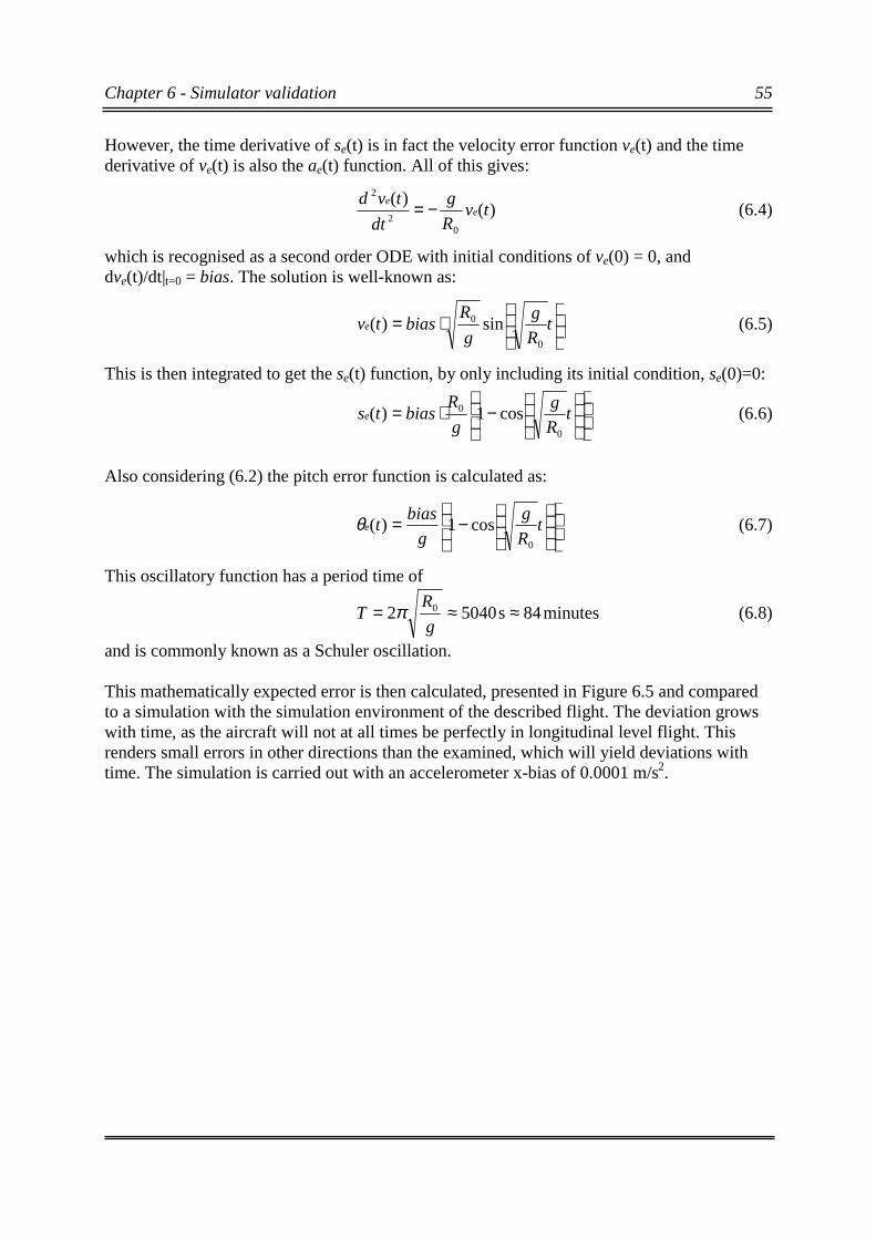
Chapter 6 - Simulator validation 55
However, the time derivative of se(t) is in fact the velocity error function ve(t) and the timederivative of ve(t) is also the ae(t) function. All of this gives:
)()(
02
2
tvR
g
dt
tvde
e −= (6.4)
which is recognised as a second order ODE with initial conditions of ve(0) = 0, anddve(t)/dt|t=0 = bias. The solution is well-known as:
⋅= t
R
g
g
Rbiastve
0
0 sin)( (6.5)
This is then integrated to get the se(t) function, by only including its initial condition, se(0)=0:
−⋅= t
R
g
g
Rbiastse
0
0 cos1)( (6.6)
Also considering (6.2) the pitch error function is calculated as:
−= t
R
g
g
biaste
0
cos1)(θ (6.7)
This oscillatory function has a period time of
minutes84s50402 0 ≈≈=g
RT π (6.8)
and is commonly known as a Schuler oscillation.
This mathematically expected error is then calculated, presented in Figure 6.5 and comparedto a simulation with the simulation environment of the described flight. The deviation growswith time, as the aircraft will not at all times be perfectly in longitudinal level flight. Thisrenders small errors in other directions than the examined, which will yield deviations withtime. The simulation is carried out with an accelerometer x-bias of 0.0001 m/s2.
Chapter 6 - Simulator validation 56
Initial pitch errorAn error similar to the accelerometer bias is if an initial pitch error in the INS is present. Infact the exact same ODE is the result, but with other initial conditions. The initial conditionsfor this ODE is, dve(t)/dt = -gsinθe(0) where θe(0) is the initial pitch error. This together withthe ODE above yields the following error functions:
−= t
R
ggRtv ee
00 sin)0()( θ (6.9)
−
= 1cos)0()(
00 t
R
gRts ee θ (6.10)
=+= t
R
g
R
tst e
eee
00
cos)0()(
)0()( θθθ (6.11)
The simulated versus calculated values with an initial pitch error of 0.0001 radians arepresented in Figure 6.6 below.
The calculated and simulated errors does not differ much at any time of simulation, whichyields that the navigation properties of the system is validated with respect to this error.
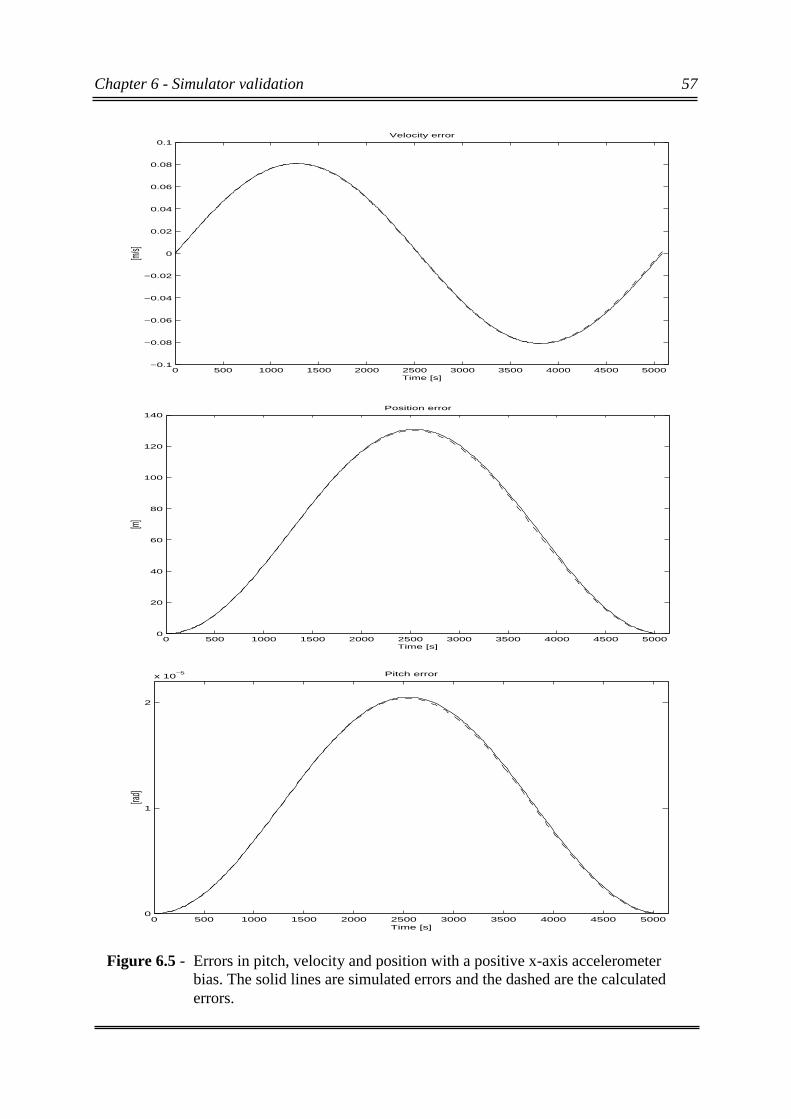
Chapter 6 - Simulator validation 57
Figure 6.5 - Errors in pitch, velocity and position with a positive x-axis accelerometerbias. The solid lines are simulated errors and the dashed are the calculatederrors.
0 500 1000 1500 2000 2500 3000 3500 4000 4500 5000−0.1
−0.08
−0.06
−0.04
−0.02
0
0.02
0.04
0.06
0.08
0.1Velocity error
Time [s]
[m/s]
0 500 1000 1500 2000 2500 3000 3500 4000 4500 50000
20
40
60
80
100
120
140Position error
Time [s]
[m]
0 500 1000 1500 2000 2500 3000 3500 4000 4500 50000
1
2
x 10−5 Pitch error
Time [s]
[rad]
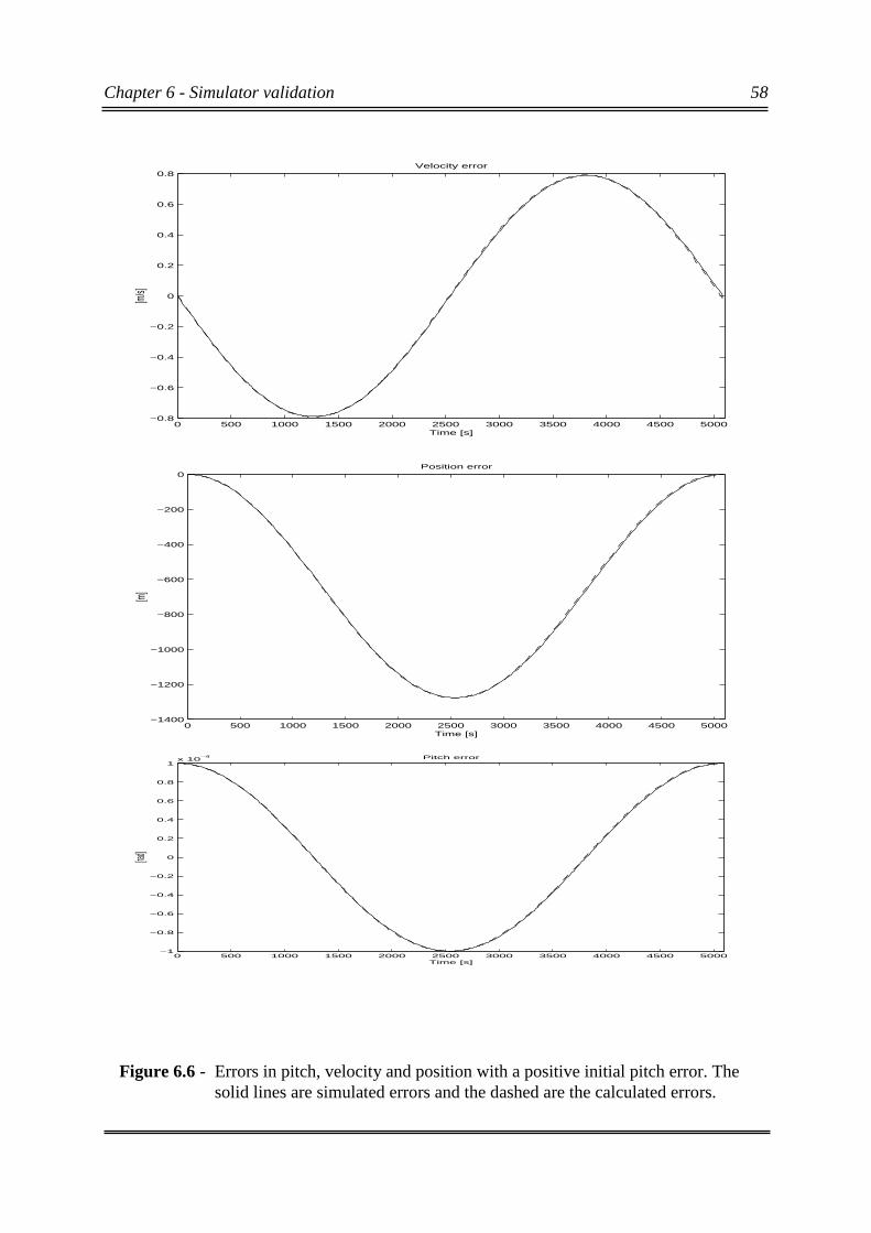
Chapter 6 - Simulator validation 58
0 500 1000 1500 2000 2500 3000 3500 4000 4500 5000−0.8
−0.6
−0.4
−0.2
0
0.2
0.4
0.6
0.8Velocity error
Time [s]
[m/s]
0 500 1000 1500 2000 2500 3000 3500 4000 4500 5000−1400
−1200
−1000
−800
−600
−400
−200
0Position error
Time [s]
[m]
0 500 1000 1500 2000 2500 3000 3500 4000 4500 5000−1
−0.8
−0.6
−0.4
−0.2
0
0.2
0.4
0.6
0.8
1x 10
−4 Pitch error
Time [s]
[rad]
Figure 6.6 - Errors in pitch, velocity and position with a positive initial pitch error. Thesolid lines are simulated errors and the dashed are the calculated errors.

Chapter 6 - Simulator validation 59
Gyro bias around y-axisAnother similar error is a pitch rate gyro bias which will also yield a Schuler oscillation, butnot according to the same ODE. The time derivative of the pitch error will instead be:
0
)()(
R
tvbias
dt
td ee +=θ(6.12)
where the gyro bias is denoted by bias.
The time derivative will then be, again remembering that the bias is constant:
002
2 )()(1)(
R
tg
dt
tdv
Rdt
td eee θθ −== (6.13)
and together with the initial conditions θe(0)=0 and dθe(0)/dt = bias, the solution of this ODEis:
= t
R
g
g
Rbiaste
0
0 sin)(θ (6.14)
and solving for ve(t) with ve(0)=0 gives:
−
⋅= 1cos)(
00 t
R
gRbiastve (6.15)
Finally the expression for the se(t) function is deduced, by considering that se(0) = 0 andintegrate the last equation as ve(t) = dse(t)/dt.
−
⋅= tt
R
g
g
RRbiastse
0
00 sin)( (6.16)
The position error function se(t) will apparently include a term which is growing with time,which means the Schuler oscillation is superpositioned upon this error. This is presented inFigure 6.7. The gyro bias in the pitch rate gyro is 1⋅10-8 [rad/s].
Again the difference is very small and the system is validated with respect to these errors.

Chapter 6 - Simulator validation 60
0 500 1000 1500 2000 2500 3000 3500 4000 4500 5000−0.14
−0.12
−0.1
−0.08
−0.06
−0.04
−0.02
0Velocity error
Time [s]
[m/s]
0 500 1000 1500 2000 2500 3000 3500 4000 4500 5000−350
−300
−250
−200
−150
−100
−50
0Position error
Time [s]
[m]
0 500 1000 1500 2000 2500 3000 3500 4000 4500 5000−1
−0.8
−0.6
−0.4
−0.2
0
0.2
0.4
0.6
0.8
1x 10
−5 Pitch error
Time [s]
[rad]
Figure 6.7 - Errors in pitch, velocity and position with a positive gyro y-axis error. Thesolid lines are simulated errors and the dashed are the calculated errors.
Chapter 6 - Simulator validation 61
6.2.2 Errors orthogonal to the direction of travelThese errors are primarily errors in gyro measurements in roll and yaw, and accelerometererror in the y-axis direction. The errors that result from these sensor errors are roll angle error,yaw angle error and velocity and position errors in the y-axis, pointing out of the right wing.
The roll error is denoted φe(t), the yaw error ψe(t), the velocity error ve(t) and the positionerror se(t). If a roll error is present the INS will have an error in its local reference which willyield error components of both the earth rotation and the rotation due to the aircraft movingalong the elliptic earth. As the assumption is flight on the equatorial line, these will at alltimes of flight be directed towards the north pole, and will then yield an error in the derivativeof the yaw angle. In the same way, an error in yaw, will yield an error in the derivative of theroll angle. This rotation's magnitude is (We + v/R0).
Also if an error in the velocity estimate is present, there will be an error in the INScorresponding to calculating the aircraft's moving rotation wrong. In the roll error derivative,a corresponding term of ve(t)/R0 has to be added to estimate this. Also in the yaw angle errorderivative calculation, an error in position will render a contribution of calculating the latitudedependent earth and aircraft's moving rotations wrong.
If all of these assumptions are collected, these coupled differential equations will be theresults:
000
00
)()()(
)()(
)()(
)()(
)()(
)()(
R
ts
R
tvWt
R
tvWgbias
dt
td
gbiasR
tvt
R
tvW
dt
td
tvdt
tds
abiastgdt
tdv
eeeez
e
xe
ee
e
ee
yee
+−
+−=
+−
+=
=
+=
φψ
ψφ
φ
(6.17)
where v(t) is the true longitudinal speed relative to ground.
In Figures (6.8-6.10) simulations vs calculated errors are presented. The sensor errorssimulated are gyro-bias of 1⋅10-8 rad/s in roll-rate measures, gbiasx, gyro-bias of 1⋅10-8 rad/s inyaw-rate measures gbiasz and accelerometer bias of 1⋅10-4 m/s2 in body y-axis, abiasy.
The differences (in the first two examples) are somewhat larger here, due to the rather harshsimplifications made in the theoretical analysis of these errors. Still, none of the plots differmuch and no question of the validity of the system arises.
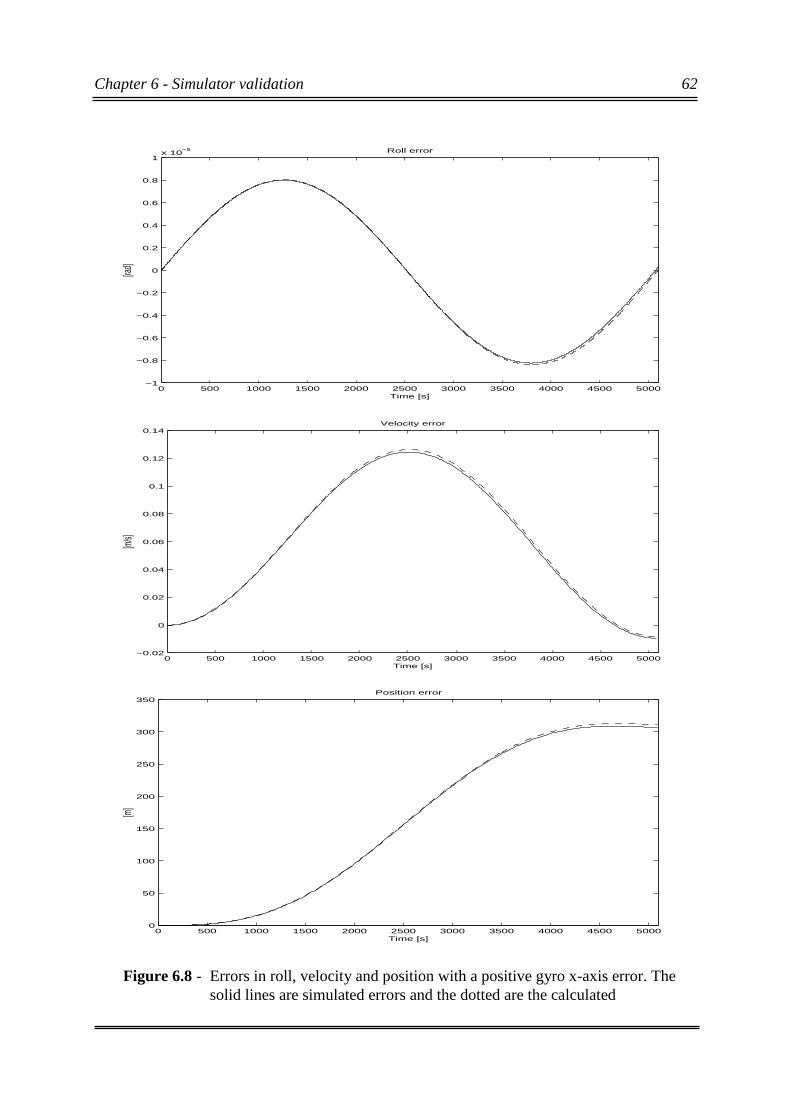
Chapter 6 - Simulator validation 62
Figure 6.8 - Errors in roll, velocity and position with a positive gyro x-axis error. Thesolid lines are simulated errors and the dotted are the calculated
0 500 1000 1500 2000 2500 3000 3500 4000 4500 5000−1
−0.8
−0.6
−0.4
−0.2
0
0.2
0.4
0.6
0.8
1x 10
−5 Roll error
Time [s]
[rad]
0 500 1000 1500 2000 2500 3000 3500 4000 4500 5000−0.02
0
0.02
0.04
0.06
0.08
0.1
0.12
0.14Velocity error
Time [s]
[m/s]
0 500 1000 1500 2000 2500 3000 3500 4000 4500 50000
50
100
150
200
250
300
350Position error
Time [s]
[m]

Chapter 6 - Simulator validation 63
Figure 6.9- Errors in yaw, velocity and position with a positive gyro z-axis error. Thesolid lines are simulated errors and the dashed are the calculated
0 500 1000 1500 2000 2500 3000 3500 4000 4500 50000
0.5
1
1.5
2
2.5
3
3.5
4
4.5
5x 10
−5 Yaw error
Time [s]
[rad]
0 500 1000 1500 2000 2500 3000 3500 4000 4500 5000−0.005
0
0.005
0.01
0.015
0.02
0.025
0.03
0.035Velocity error
Time [s]
[m/s]
0 500 1000 1500 2000 2500 3000 3500 4000 4500 50000
10
20
30
40
50
60
70
80
90Position error
Time [s]
[m]
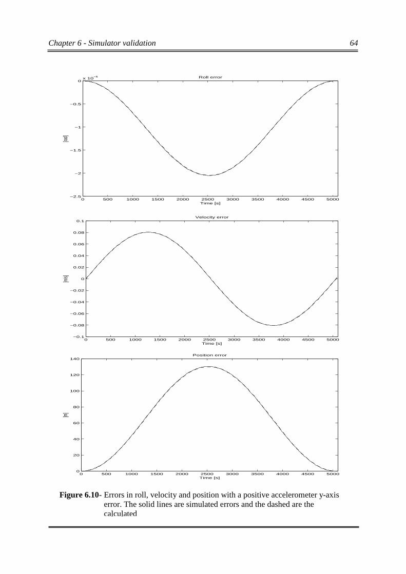
Chapter 6 - Simulator validation 64
Figure 6.10- Errors in roll, velocity and position with a positive accelerometer y-axiserror. The solid lines are simulated errors and the dashed are thecalculated
0 500 1000 1500 2000 2500 3000 3500 4000 4500 5000−2.5
−2
−1.5
−1
−0.5
0x 10
−5 Roll error
Time [s]
[rad]
0 500 1000 1500 2000 2500 3000 3500 4000 4500 5000−0.1
−0.08
−0.06
−0.04
−0.02
0
0.02
0.04
0.06
0.08
0.1Velocity error
Time [s]
[m/s]
0 500 1000 1500 2000 2500 3000 3500 4000 4500 50000
20
40
60
80
100
120
140Position error
Time [s]
[m]

Chapter 6 - Simulator validation 65
6.2.3 Errors resulting from attitude changesWhen attitude is constant, sensor errors as scale factor error and misalignment give the exactsame effect as the constant bias. If attitude is constant the bias values is a mere combinationof the three errors, bias, scale factor and misalignment. A validation of these errors under thisassumption would be an exact repetition of the validation performed earlier in this chapter. Tovalidate these errors, attitude must vary over time, i.e. the aircraft has to make changes in roll,heading and also in pitch. The attitude errors resulting from these can then be compared toerror equations, where these sensor errors are modelled.
Expressing differential equations for the Euler angles describing the attitude develops theseerror equations. Remember the definition of the attitude angles:
Yaw, ψ, is the angle between the local frame's x-axis and the projection of the body x-axis inthe horizontal plane. This makes the yaw derivative, dψ/dt, if expressed as a vector to bedirected in the local level z-axis.
Pitch, θ, is the angle between the horizontal and the body x-axis, measured in the verticalplane. The pitch derivative dθ/dt is then a vector along the local level y-axis rotated with theyaw angle.
Roll, φ, is the angle between the local level y-axis and the aircraft y-axis measured in the locallevel yz-plane. The roll derivative, dφ/dt, then is a vector along the body x-axis.
The rotations performed by the aircraft are described in the body frame with respect to theinertial reference, and are expressed as [P Q R]. Projecting the attitude derivatives along thebody axes will then yield the following expressions:
φθφθψφθψφθ
θψφ
sincoscos
sincoscos
sin
��
��
��
−=
+=
−=
R
Q
P
(6.18)
These equations are then used to solve for the Euler angle state derivatives:
θφ
θφψ
θφθφφφφθ
cos
cos
cos
sin
tancostansin
sincos
RQ
RQP
RQ
+=
++=
−=
�
�
�
(6.19)
These are then derived with respect to the attitude angles, to get a first-order error form.Biases in gyroscopes are transformed directly into the error equations according to equation(6.19). The full error equations are presented below, denoting the errors: φe(t), θe(t), ψe(t):
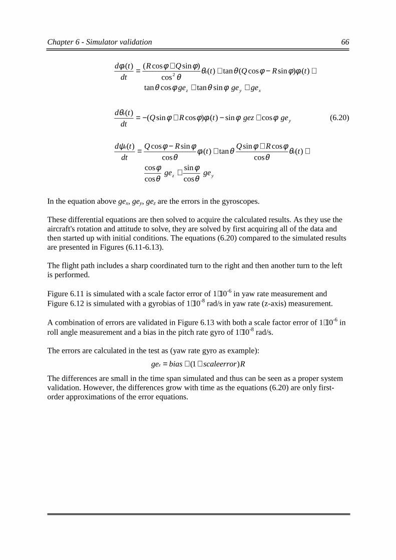
Chapter 6 - Simulator validation 66
yz
eee
yee
xyz
eee
gege
tRQ
tRQ
dt
td
gegeztRQdt
td
gegege
tRQtQR
dt
td
θφ
θφ
θθ
φφθφθ
φφψ
φφφφφθ
φθφθ
φφφθθθ
φφφ
cos
sin
cos
cos
)(cos
cossintan)(
cos
sincos)(
cossin)()cossin()(
sintancostan
)()sincos(tan)(cos
)sincos()(2
+
+++−=
+−+−=
++
+−++=
(6.20)
In the equation above gex, gey, gez are the errors in the gyroscopes.
These differential equations are then solved to acquire the calculated results. As they use theaircraft's rotation and attitude to solve, they are solved by first acquiring all of the data andthen started up with initial conditions. The equations (6.20) compared to the simulated resultsare presented in Figures (6.11-6.13).
The flight path includes a sharp coordinated turn to the right and then another turn to the leftis performed.
Figure 6.11 is simulated with a scale factor error of 1⋅10-6 in yaw rate measurement andFigure 6.12 is simulated with a gyrobias of 1⋅10-8 rad/s in yaw rate (z-axis) measurement.
A combination of errors are validated in Figure 6.13 with both a scale factor error of 1⋅10-6 inroll angle measurement and a bias in the pitch rate gyro of 1⋅10-8 rad/s.
The errors are calculated in the test as (yaw rate gyro as example):
Rscaleerrorbiasgez )1( ++=
The differences are small in the time span simulated and thus can be seen as a proper systemvalidation. However, the differences grow with time as the equations (6.20) are only first-order approximations of the error equations.
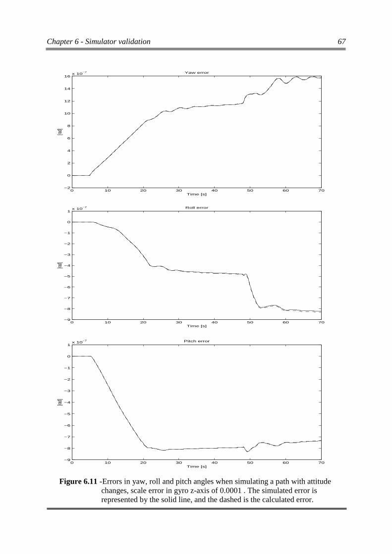
Chapter 6 - Simulator validation 67
Figure 6.11 -Errors in yaw, roll and pitch angles when simulating a path with attitudechanges, scale error in gyro z-axis of 0.0001 . The simulated error isrepresented by the solid line, and the dashed is the calculated error.
0 10 20 30 40 50 60 70−2
0
2
4
6
8
10
12
14
16x 10
−7 Yaw error
Time [s]
[rad]
0 10 20 30 40 50 60 70−9
−8
−7
−6
−5
−4
−3
−2
−1
0
1x 10
−7 Roll error
Time [s]
[rad]
0 10 20 30 40 50 60 70−9
−8
−7
−6
−5
−4
−3
−2
−1
0
1x 10
−7 Pitch error
Time [s]
[rad]
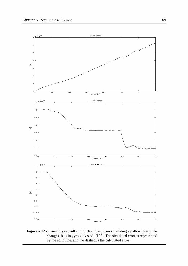
Chapter 6 - Simulator validation 68
Figure 6.12 -Errors in yaw, roll and pitch angles when simulating a path with attitudechanges, bias in gyro z-axis of 1⋅10-8 . The simulated error is representedby the solid line, and the dashed is the calculated error.
0 10 20 30 40 50 60 700
1
2
3
4
5
6
7x 10
−7 Yaw error
Time [s]
[rad]
0 10 20 30 40 50 60 70−12
−10
−8
−6
−4
−2
0
2x 10
−8 Roll error
Time [s]
[rad]
0 10 20 30 40 50 60 70−16
−14
−12
−10
−8
−6
−4
−2
0
2x 10
−8 Pitch error
Time [s]
[rad]
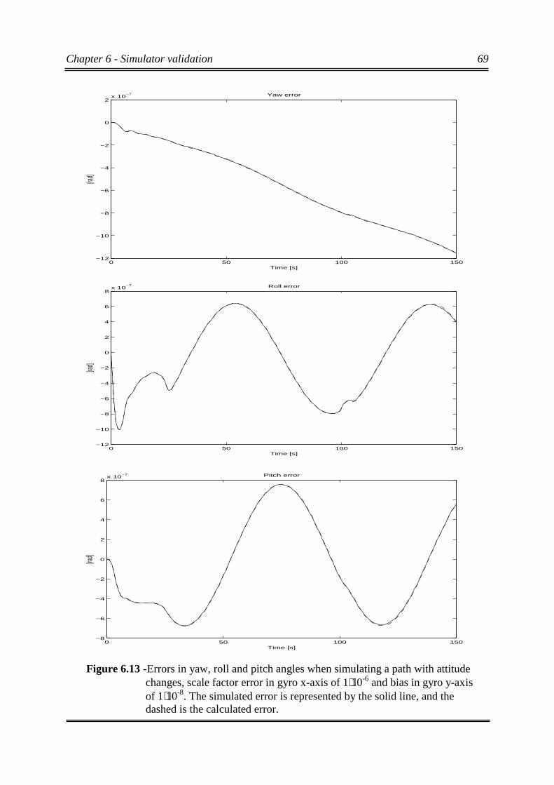
Chapter 6 - Simulator validation 69
Figure 6.13 -Errors in yaw, roll and pitch angles when simulating a path with attitudechanges, scale factor error in gyro x-axis of 1⋅10-6 and bias in gyro y-axisof 1⋅10-8. The simulated error is represented by the solid line, and thedashed is the calculated error.
0 50 100 150−12
−10
−8
−6
−4
−2
0
2x 10
−7 Yaw error
Time [s]
[rad]
0 50 100 150−12
−10
−8
−6
−4
−2
0
2
4
6
8x 10
−7 Roll error
Time [s]
[rad]
0 50 100 150−8
−6
−4
−2
0
2
4
6
8x 10
−7 Pitch error
Time [s]
[rad]
Chapter 7 - Discussion 70
Chapter 7
ConclusionsThe choice of Simulink as the development environment has given the advantages of greatflexibility. Any navigational approach can be tested, if made as a Simulink block and thenconnected to the Navigational Simulator, without having to write any code. Also nounderstanding of the theory and practical implementation of the Navigational Simulator isneeded to use it.
The speed of simulation varies by choice of solver and error tolerances and also by whichsubsystems and external blocks that are used. It is in the range of 120 - 200 % of real time(measured at an Ultra Sparcstation 30, using the suggested solver from Section 3.6 and usingan external INS as the only external navigational block). This is enough for single simulationsto be evaluated, but of course speed improvements are always desired. For instance, if Monte-Carlo simulations are to be made with the simulator, this speed makes the work tedious. Amore error tolerant or even a fixed-step solver is then suggested to be used.
To avoid undetected numerical errors, two state update algorithms are used (by choice, ifspeed is a priority it can be deselected in the GUI). This yields warnings when solutions startto differ. If a warning is issued, the data produced by the simulator should be examined morethoroughly before accepting it as a good estimate of the algorithms being evaluated. This isalso only a test, which may find numerical problems, it does not detect all numericalproblems.
The implementation of the Terrain Database (originally from Saab Dynamics) routines wererewritten to fit in a Simulink block (with a reasonable speed). This work also produced a newapproach in using the Terrain Database, which improved access speeds with 300 percent.
The equations of motion, developed with the non-rotating earth as inertial frame has proven tobe quite adequate for the simulator, as the rotation of the earth and thereby resulting Coriolisaccelerations are compensated for prior to sensor output. However it will make the aircraft flya little less realistic as the dynamics does not include these properties.
The guidance logic used is good enough for waypoints separated by at least the aircraft’sturning radius when flying in the comfortable Waypoint control mode. When waypoints aretoo closely put, the aircraft will start circling the waypoint until the tolerance is met. This israrely the intended behaviour, but would require an alternative algorithm built into theguidance logic.
The library of navigation sources include several different blocks (GPS, DGPS, INS) and alsoa (quite) general Kalman Filter has been developed to be used in sensor fusion.

Chapter 7 - Discussion 71
Control of the aircraft as performed by the PID-like controller circuits works well in thevelocity ranges of 50-290 m/s and at most altitudes. When the aircraft enters the trans-sonicarea, problems do occur and the closed-loop system gets unstable at times. This is not fullysolved in this master thesis. Although this might be a problem, once the aircraft leaves thetrans-sonic area, either side, the controller again stabilises it. This only applies if thecontroller has not caused instability during the process of transporting the vehicle through thetrans-sonic area.
The aim for user friendliness presented in the objectives are taken care of both Simulink’sintuitive and simple design methods, and by the fact that the whole environment is controlledby a point-n’-click graphical user interface. In fact, to setup a simulation no prior knowledgeof how to do it is necessary. The GUI is self-explanatory, but to a first-time user, the User’sGuide might be handy (Appendix B).
7.1 Future workA possible and desired line of future work would be to change the model from being based onthe F-16 fighter aircraft to be based on a more Gripen-like aircraft. Although the properties ofthe aircraft have little influence on navigational evaluation, it has quite some influence on theevaluation of collision avoidance systems (both mid-air and ground). In these applications theaircraft’s response time to steering commands is vital.
Another part of possible future work is to make, instead of the PID-like approach, a morerealistic and better control based on LQR-theory. This approach demands linearisations andcalculations of controllers around several different points in state space, and some kind ofscheme to select which one to use, or which combination to use (one approach is for exampleto linearly interpolate between feedback vectors). This will also have quite small influence onnavigational evaluation but much more in collision avoidance evaluation.
The guidance logic is another area of interest. It would be necessary to improve if waypointsare to be very close to each other as the present guidance logic fails then. A possible approachis to decide when such erratic behaviour is present and then provide an alternative algorithm.A simple approach at this is included in the preliminary flight path calculator, but not in theaircraft guidance logic. The idea is to decide when the aircraft increases its distance towardsthe waypoint after a threshold time, and try to first fly away from the point then reconnect theoriginal guidance logic. This will yield somewhat better flightpaths, yet not in any wayoptimal.
More navigational system blocks also has to be developed (example: TERNAV, TARAS etc)to be used in the development of sensor fusion algorithms. This work is done for someestimate sources (GPS, DGPS, INS). When more sources are modelled, an update of thesimulator environment graphical user interface to auto-initialise these new blocks would beneeded.
References 72
References
[1] ”Dynamics of Flight - Stability and Control 3rd Edition”Bernard Etkin / Lloyd Duff ReidJohn Wiley & Sons Inc, 1996
[2] ”Automatic Control of Aircraft and Missiles 2nd Edition”John H. BlakelockJohn Wiley & Sons Inc, 1991
[3] ”Modeling of dynamic systems”Lennart Ljung / Torkel GladP T R Prentice Hall, 1994
[4] ”Reglerteori”Lennart Ljung / Torkel GladStudentlitteratur, 1997
[5] ”An environment for simulation of inertial navigation and a method forintegration of inertial navigation system and GPS”Per-Johan NordlundMaster thesis at Linköping University, LiTH-ISY-EX-1728, 1996
[6] ”Graceful degradation of an integrated navigation system and improvement ofan INS simulator”Magnus AnderssonMaster thesis at Linköping University, LiTH-ISY-EX-1834, 1997
[7] ”Digital styrning - kurskompendium”Torkel Glad / Svante Gunnarsson / Lennart Ljung / Tomas McKelveyLinköping University, Department of AutomaticControl, 1999
[8] "Inertial Navigation Systems"Charles BroxmeyerMcGraw-Hill, Inc. 1964
[9] "Quaternions and rotation sequences, a primer with applications toorbits, aerospace and virtual reality"Jack B. KuipersPrinceton University Press, cop. 1999
Appendix A - Notation used
AbbreviationsINS Inertial Navigation SystemGPS Global Positioning SystemDGPS Differential Global Positioning SystemTERNAV Terrain NavigationNED North-East-Down local level frameWGS-84 World Geodetic SystemGCAS Ground Collision Avoidance System
Symbolsl, L, h Position - latitude, longitude and altitudeφ, θ, ψ Attitude - roll, pitch, yawα Attack angle, aerodynamic variableβ Sideslip angle, aerodynamic variableU, V, W Velocity components in body axesP, Q, R Rotational components in body axesvN, vE, vZ Velocity components in local level NED-frameCBL Transformational matrix from B-frame to L-frameWe Rotation of the E-frame relative to the I-framewIL Rotation of the L-frame relative the I-framewIB Rotation of the body frame relative to the I-framegpb Plumb bob gravity
Coordinate framesI-frame Inertial frameE-frame Earth frameL-frame Local level frameB-frame Body frame

Fördelning/To Ärende/Subject
Godkänd/Approved by Arkiveringsdata/File
Nyckelord/KeywordKod/Code
Telefon/Phone
IN 5
000
349
-013
Utg
3 9
9.03
allm
_eng
Fra
meM
aker
5
Datum/Date Utgåva/Issue Sida/PageUtfärdare (tj-st-bet, namn)/Issued by
Dokumentslag/Type of document Reg-nr/Reg. No.
1(24)Infoklass/Info. class
Thi
s do
cum
ent i
s th
e pr
oper
ty o
f Saa
b A
B a
nd m
ust
not b
e re
prod
uced
in a
ny fo
rm o
r di
strib
uted
to th
irdpa
rty
with
out t
he w
ritte
n co
nsen
t of S
aab
AB
.
84861
- Public -
- -
Table of contents
1 INSTALLATION 2
2 SIMULATION MODEL BUILD 3
3 SIMULATION INITIALISATION GUI 43.1 Initial states 43.2 Flight Path 53.3 Sensor Errors 73.4 Simulation Parameters 73.5 Workspace Output 9
4 SIMULATION 94.1 Normal simulation 94.2 Batch simulation 10
5 EVALUATION TOOL 105.1 Error plots 105.2 Specialised plots 12
6 EXAMPLES OF MODELS 136.1 Example_1: A simple system 136.2 Example_2a,b: Introducing GPS 146.3 Example_3: GCAS 156.4 Example_4: Sensor fusion (INS, DGPS) 16
7 BLOCK REFERENCE 177.1 Navigation Simulator 177.2 Navigation Simulator with Control Input 187.3 Inertial Navigation (C) 197.4 GPS, DGPS 207.5 EvalExportVars 217.6 Kalman Matrix Calculator 227.7 Square Root Kalman Filter 237.8 INS Correction 24
- Navigation simulator User’s guide
991021 3GDFN-EXA Stefan Ahlqvist
User’s guide GDFN-99-001

991021 3PublicGDFN-EXA Stefan Ahlqvist
User’s guide GDFN-99-001
Datum/Date Utgåva/Issue Sida/PageUtfärdare (tj-st-bet, namn)/Issued by
Dokumentslag/Type of document Reg-nr/Reg. No.
Infoklass/Info. class
2(24)
IN 5
000
349
-013
Utg
3 9
9.03
allm
_eng
Fra
meM
aker
5
1 INSTALLATION
To install the simulator environment the file ’navsim.tar.gz’ has to be available.(Current release v1.0: 706059bytes large)
1.Decompress file by issuing ’gunzip navsim.tar.gz ’
2. Unfold the directories by issuing ’tar -xvf navsim.tar ’ at the commandline.
3. The MatLab path has to include the following directories
*navsim/simulink/*navsim/simulink/parfiles/*navsim/simulink/s-files/*navsim/simulink/m-files/*navsim/sim_guis/simgui/*navsim/sim_guis/wpgui/*navsim/sim_guis/evalgui/*navsim/sim_guis/*navsim/map_db/*navsim/simsets/
The installation is now completed!
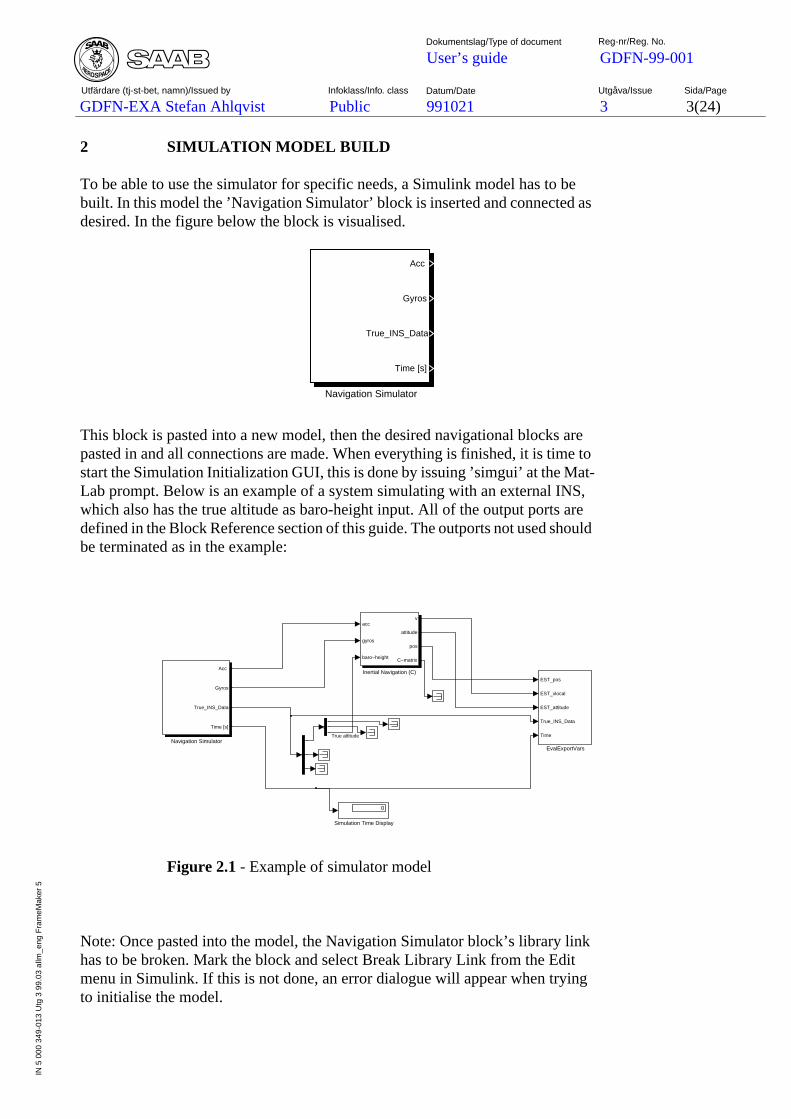
991021 3PublicGDFN-EXA Stefan Ahlqvist
User’s guide GDFN-99-001
Datum/Date Utgåva/Issue Sida/PageUtfärdare (tj-st-bet, namn)/Issued by
Dokumentslag/Type of document Reg-nr/Reg. No.
Infoklass/Info. class
3(24)
IN 5
000
349
-013
Utg
3 9
9.03
allm
_eng
Fra
meM
aker
5
2 SIMULATION MODEL BUILD
To be able to use the simulator for specific needs, a Simulink model has to bebuilt. In this model the ’Navigation Simulator’ block is inserted and connected asdesired. In the figure below the block is visualised.
This block is pasted into a new model, then the desired navigational blocks arepasted in and all connections are made. When everything is finished, it is time tostart the Simulation Initialization GUI, this is done by issuing ’simgui’ at the Mat-Lab prompt. Below is an example of a system simulating with an external INS,which also has the true altitude as baro-height input. All of the output ports aredefined in the Block Reference section of this guide. The outports not used shouldbe terminated as in the example:
Figure 2.1 - Example of simulator model
Note: Once pasted into the model, the Navigation Simulator block’s library linkhas to be broken. Mark the block and select Break Library Link from the Editmenu in Simulink. If this is not done, an error dialogue will appear when tryingto initialise the model.
Acc
Gyros
True_INS_Data
Time [s]
Navigation Simulator
0
Simulation Time Display
Acc
Gyros
True_INS_Data
Time [s]
Navigation Simulator
acc
gyros
baro−height
v
attitude
pos
C−matrix
Inertial Navigation (C)EST_pos
EST_vlocal
EST_attitude
True_INS_Data
Time
EvalExportVars
em
em
True altitude
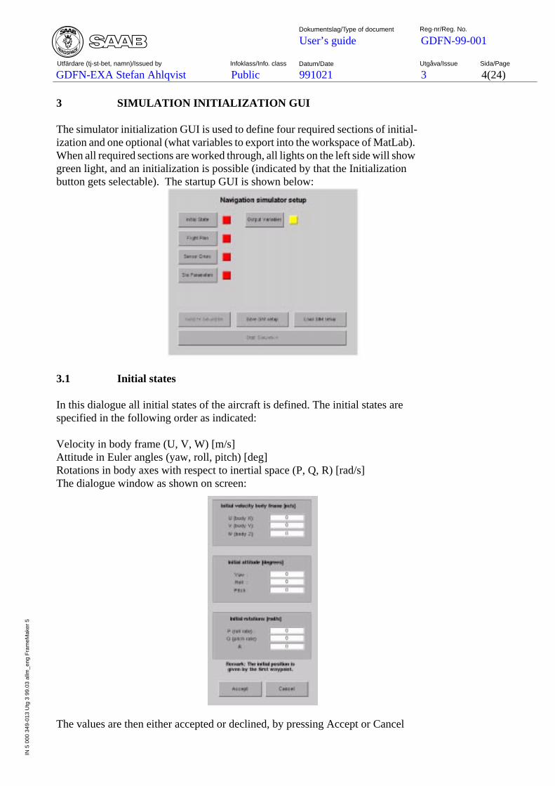
991021 3PublicGDFN-EXA Stefan Ahlqvist
User’s guide GDFN-99-001
Datum/Date Utgåva/Issue Sida/PageUtfärdare (tj-st-bet, namn)/Issued by
Dokumentslag/Type of document Reg-nr/Reg. No.
Infoklass/Info. class
4(24)
IN 5
000
349
-013
Utg
3 9
9.03
allm
_eng
Fra
meM
aker
5
3 SIMULATION INITIALIZATION GUI
The simulator initialization GUI is used to define four required sections of initial-ization and one optional (what variables to export into the workspace of MatLab).When all required sections are worked through, all lights on the left side will showgreen light, and an initialization is possible (indicated by that the Initializationbutton gets selectable). The startup GUI is shown below:
3.1 Initial states
In this dialogue all initial states of the aircraft is defined. The initial states arespecified in the following order as indicated:
Velocity in body frame (U, V, W) [m/s]Attitude in Euler angles (yaw, roll, pitch) [deg]Rotations in body axes with respect to inertial space (P, Q, R) [rad/s]The dialogue window as shown on screen:
The values are then either accepted or declined, by pressing Accept or Cancel

991021 3PublicGDFN-EXA Stefan Ahlqvist
User’s guide GDFN-99-001
Datum/Date Utgåva/Issue Sida/PageUtfärdare (tj-st-bet, namn)/Issued by
Dokumentslag/Type of document Reg-nr/Reg. No.
Infoklass/Info. class
5(24)
IN 5
000
349
-013
Utg
3 9
9.03
allm
_eng
Fra
meM
aker
5
3.2 Flight Path
This is the flight planning tool, where the waypoints are input. There are two waysto insert waypoints, the first is to fill in the fields shown and then press Insert orAdd. A sample of this flight planning GUI is shown below:
The visualizer can be setup by selecting the terrain database samples per axis, andalso what landmarks to include. Those selections are made in the top right corner.
The other is to first specify start and end-points as above and then to click the’Flight Path 2D’ button to get a map of the flight path and terrain. When the mapis shown the waypoints can be clicked in onto the map. Each click will render adialogue box where waypoint data are input and then accepted or declined. Everytime a new waypoint is inserted, the preliminary flight path gets invalid, and aquestion will be put whether to recalculate or not. A sample map is shown below(where the start-point is somewhere on the lake Vättern and the end point east ofOmberg, which is the elevated terrain passed in mid-flight):

991021 3PublicGDFN-EXA Stefan Ahlqvist
User’s guide GDFN-99-001
Datum/Date Utgåva/Issue Sida/PageUtfärdare (tj-st-bet, namn)/Issued by
Dokumentslag/Type of document Reg-nr/Reg. No.
Infoklass/Info. class
6(24)
IN 5
000
349
-013
Utg
3 9
9.03
allm
_eng
Fra
meM
aker
5
There’s also a plot of altitude versus ground altitude, and crash warnings will beissued when the aircraft is preliminary below the ground at any time of flight.Here time estimates of when the aircraft will arrive at different waypoints also canbe read out.
The waypoints can be rearranged in respect to order by using the arrow buttonsjust right of the list of waypoint names. This will bubble them up respectivelydown in the list. A waypoint is deleted when delete is pressed, and all waypointsare deleted when Clear is pressed.
After updating a parameter of a waypoint (by clicking on it in the list and then editthe appropriate value) the button Update has to be pressed, otherwise the changeis cancelled.
When satisfied with the waypoints, the Accept button is pressed to return to thesimulator GUI. If the Cancel button is clicked, NO changes are made, and no pre-liminary flightpath is exported to the simulator GUI (this is important when theevaluation GUI is used, where a preliminary flightpath is assumed to have beencalculated). Also remember, if waypoints are altered after a visualization is done,the preliminary path will be invalid.
Each waypoint also has a Flight Mode parameter and a tolerance parameter.Flight Mode is either Waypoint or Terrain Follow, with Terrain Follow using amuch stricter policy for altitude hold. Default is Waypoint mode. Tolerance is theaccepted distance to the waypoint when to regard the waypoint as fulfilled andstart guiding towards next waypoint. Default is 200 metres.
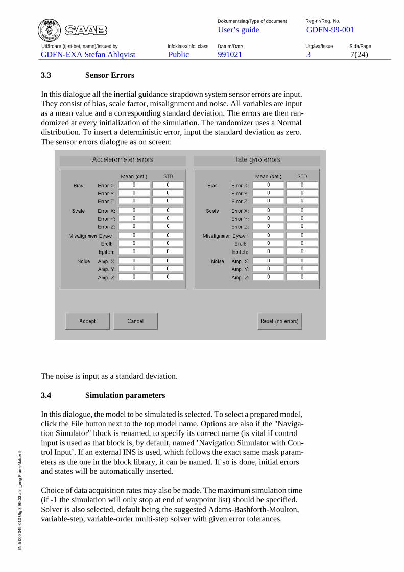
991021 3PublicGDFN-EXA Stefan Ahlqvist
User’s guide GDFN-99-001
Datum/Date Utgåva/Issue Sida/PageUtfärdare (tj-st-bet, namn)/Issued by
Dokumentslag/Type of document Reg-nr/Reg. No.
Infoklass/Info. class
7(24)
IN 5
000
349
-013
Utg
3 9
9.03
allm
_eng
Fra
meM
aker
5
3.3 Sensor Errors
In this dialogue all the inertial guidance strapdown system sensor errors are input.They consist of bias, scale factor, misalignment and noise. All variables are inputas a mean value and a corresponding standard deviation. The errors are then ran-domized at every initialization of the simulation. The randomizer uses a Normaldistribution. To insert a deterministic error, input the standard deviation as zero.The sensor errors dialogue as on screen:
The noise is input as a standard deviation.
3.4 Simulation parameters
In this dialogue, the model to be simulated is selected. To select a prepared model,click the File button next to the top model name. Options are also if the "Naviga-tion Simulator" block is renamed, to specify its correct name (is vital if controlinput is used as that block is, by default, named ’Navigation Simulator with Con-trol Input’. If an external INS is used, which follows the exact same mask param-eters as the one in the block library, it can be named. If so is done, initial errorsand states will be automatically inserted.
Choice of data acquisition rates may also be made. The maximum simulation time(if -1 the simulation will only stop at end of waypoint list) should be specified.Solver is also selected, default being the suggested Adams-Bashforth-Moulton,variable-step, variable-order multi-step solver with given error tolerances.

991021 3PublicGDFN-EXA Stefan Ahlqvist
User’s guide GDFN-99-001
Datum/Date Utgåva/Issue Sida/PageUtfärdare (tj-st-bet, namn)/Issued by
Dokumentslag/Type of document Reg-nr/Reg. No.
Infoklass/Info. class
8(24)
IN 5
000
349
-013
Utg
3 9
9.03
allm
_eng
Fra
meM
aker
5
Finally, a choice of which subsystems to run during simulation has to be made.The simple rule is, more subsystems less simulation speed. Hence if Monte Carlosimulations are made (preferrably by using the batch program explained in Sec-tion 5) as few subsystems as possible should be enabled).
Available subsystems (to date) is GCAS (Ground Collision Avoidance), GroundCrash Detection (if GCAS is used, this might also be useful), Numerical ErrorSupervisor (yields warnings after simulating if significant numerical errors areencountered). Also Control Input should be checked here if used to inform theenvironment what block is used (WILL not automatically change blocks!). Anoptional instrument panel showing a pitch & roll instrument, GCAS warninglamp and also a map following the aircraft’s position can be selected by checkingthe Instrument Panel button.
These changes of parameters can also be either accepted or cancelled. Below ishow the dialogue looks on screen:
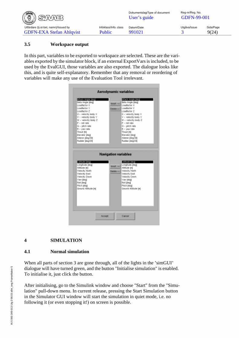
991021 3PublicGDFN-EXA Stefan Ahlqvist
User’s guide GDFN-99-001
Datum/Date Utgåva/Issue Sida/PageUtfärdare (tj-st-bet, namn)/Issued by
Dokumentslag/Type of document Reg-nr/Reg. No.
Infoklass/Info. class
9(24)
IN 5
000
349
-013
Utg
3 9
9.03
allm
_eng
Fra
meM
aker
5
3.5 Workspace output
In this part, variables to be exported to workspace are selected. These are the vari-ables exported by the simulator block, if an external ExportVars is included, to beused by the EvalGUI, those variables are also exported. The dialogue looks likethis, and is quite self-explanatory. Remember that any removal or reordering ofvariables will make any use of the Evaluation Tool irrelevant.
4 SIMULATION
4.1 Normal simulation
When all parts of section 3 are gone through, all of the lights in the ’simGUI’dialogue will have turned green, and the button "Initialise simulation" is enabled.To initialise it, just click the button.
After initialising, go to the Simulink window and choose "Start" from the "Simu-lation" pull-down menu. In current release, pressing the Start Simulation buttonin the Simulator GUI window will start the simulation in quiet mode, i.e. nofollowing it (or even stopping it!) on screen is possible.

991021 3PublicGDFN-EXA Stefan Ahlqvist
User’s guide GDFN-99-001
Datum/Date Utgåva/Issue Sida/PageUtfärdare (tj-st-bet, namn)/Issued by
Dokumentslag/Type of document Reg-nr/Reg. No.
Infoklass/Info. class
10(24)
IN 5
000
349
-013
Utg
3 9
9.03
allm
_eng
Fra
meM
aker
5
After the simulation is finished, all selected variables will be available in the baseworkspace of MatLab.
4.2 Batch simulation
If batch simulations are preferred, to make Monte Carlo simulation of the samemodel, usage of the batchsim program is suggested. First, though, the simulationmodel has to be initialised by pressing the initialisation button.
Then put the marker in a MatLab window, and run:batchsim(model, sims, dec_rate, max_time, initfile)wheremodel is the top model name of the model to be simulated,noofsimsare the number of simulations anddec_rate is the decimation rate at whichdata is remembered to create the RMS estimates. Optional arguments aremax_time which is a maximum simulation time andinitfile which is the.nsm file used to initialise the model If initfile is not specified, it will as-sume that the initialisation file is available as ’model ’ .nsm
Example:
batchsim(’simINS’, 25, 16)
will open the ’simINS’ model, initialise it with the initialisation file ’simINS.nsm’(which has exist on the MatLab path) and simulate it 25 times and collect dataeach time decimated by a factor 16 (if the data acquisition rate is 1 sec, data willbe collected every 16 seconds). After the simulation is finished, the workspacewill contain RMS estimates of all variables exported from the model. It will beplaced in the workspace variable RMS_Errors.
5 EVALUATION TOOL
The Evaluation Tool may be run to evaluate a simulation after it has been runthrough. It will check if the data needed is available in the current MatLab work-space. If not, something might have been initialised wrong. Check that the Work-space Output is exactly as stated in the example dialogue from section 3.5.
5.1 Error plots
The first column of buttons (three first) will yield plots of position, attitude andvelocity component-wise. It will plot true data against the estimated data sent intothe "EvalExportVars" block. Note: if the baro-height block is used, true altitudewill differ from the estimated although no sensor errors are present.
The fourth button will render a horizontal plot of the true position, estimated po-sition and also of the preliminary flight path as calculated before the simulation.
An example of such a plot is shown below (position plot):
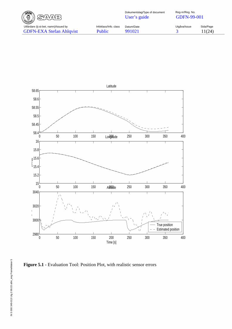
991021 3PublicGDFN-EXA Stefan Ahlqvist
User’s guide GDFN-99-001
Datum/Date Utgåva/Issue Sida/PageUtfärdare (tj-st-bet, namn)/Issued by
Dokumentslag/Type of document Reg-nr/Reg. No.
Infoklass/Info. class
11(24)
IN 5
000
349
-013
Utg
3 9
9.03
allm
_eng
Fra
meM
aker
5
Figure 5.1- Evaluation Tool: Position Plot, with realistic sensor errors
0 50 100 150 200 250 300 350 40058.4
58.45
58.5
58.55
58.6
58.65Latitude
0 50 100 150 200 250 300 350 40015
15.2
15.4
15.6
15.8
16Longitude
[de
g]
0 50 100 150 200 250 300 350 4002980
3000
3020
3040Altitude
[]
Time [s]
True position Estimated position
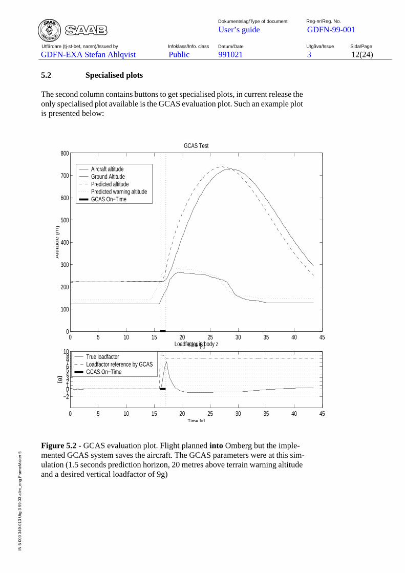
991021 3PublicGDFN-EXA Stefan Ahlqvist
User’s guide GDFN-99-001
Datum/Date Utgåva/Issue Sida/PageUtfärdare (tj-st-bet, namn)/Issued by
Dokumentslag/Type of document Reg-nr/Reg. No.
Infoklass/Info. class
12(24)
IN 5
000
349
-013
Utg
3 9
9.03
allm
_eng
Fra
meM
aker
5
5.2 Specialised plots
The second column contains buttons to get specialised plots, in current release theonly specialised plot available is the GCAS evaluation plot. Such an example plotis presented below:
Figure 5.2 - GCAS evaluation plot. Flight planned into Omberg but the imple-mented GCAS system saves the aircraft. The GCAS parameters were at this sim-ulation (1.5 seconds prediction horizon, 20 metres above terrain warning altitudeand a desired vertical loadfactor of 9g)
0 5 10 15 20 25 30 35 40 450
100
200
300
400
500
600
700
800GCAS Test
Time [s]
Altitu
de
[m
]
Aircraft altitude Ground Altitude Predicted altitude Predicted warning altitudeGCAS On−Time
0 5 10 15 20 25 30 35 40 45
−2−1012345678910
Loadfactor in body z
Time [s]
[g]
True loadfactor Loadfactor reference by GCASGCAS On−Time
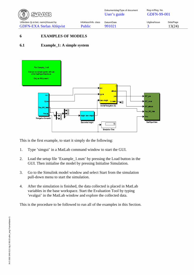
991021 3PublicGDFN-EXA Stefan Ahlqvist
User’s guide GDFN-99-001
Datum/Date Utgåva/Issue Sida/PageUtfärdare (tj-st-bet, namn)/Issued by
Dokumentslag/Type of document Reg-nr/Reg. No.
Infoklass/Info. class
13(24)
IN 5
000
349
-013
Utg
3 9
9.03
allm
_eng
Fra
meM
aker
5
6 EXAMPLES OF MODELS
6.1 Example_1: A simple system
This is the first example, to start it simply do the following:
1. Type ’simgui’ in a MatLab command window to start the GUI.
2. Load the setup file ’Example_1.nsm’ by pressing the Load button in theGUI. Then initialise the model by pressing Initialise Simulation.
3. Go to the Simulink model window and select Start from the simulationpull-down menu to start the simulation.
4. After the simulation is finished, the data collected is placed in MatLabvariables in the base workspace. Start the Evaluation Tool by typing’evalgui’ in the MatLab window and explore the collected data.
This is the procedure to be followed to run all of the examples in this Section.
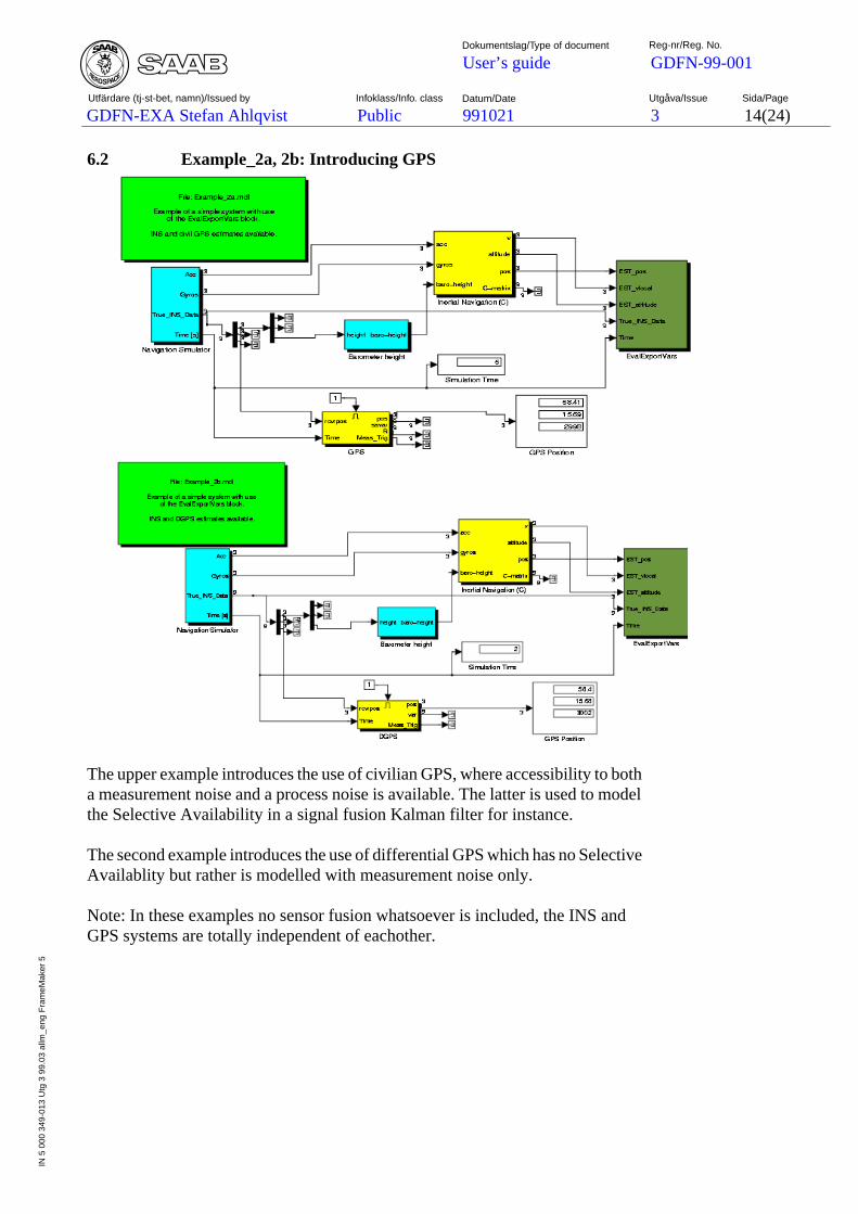
991021 3PublicGDFN-EXA Stefan Ahlqvist
User’s guide GDFN-99-001
Datum/Date Utgåva/Issue Sida/PageUtfärdare (tj-st-bet, namn)/Issued by
Dokumentslag/Type of document Reg-nr/Reg. No.
Infoklass/Info. class
14(24)
IN 5
000
349
-013
Utg
3 9
9.03
allm
_eng
Fra
meM
aker
5
6.2 Example_2a, 2b: Introducing GPS
The upper example introduces the use of civilian GPS, where accessibility to botha measurement noise and a process noise is available. The latter is used to modelthe Selective Availability in a signal fusion Kalman filter for instance.
The second example introduces the use of differential GPS which has no SelectiveAvailablity but rather is modelled with measurement noise only.
Note: In these examples no sensor fusion whatsoever is included, the INS andGPS systems are totally independent of eachother.
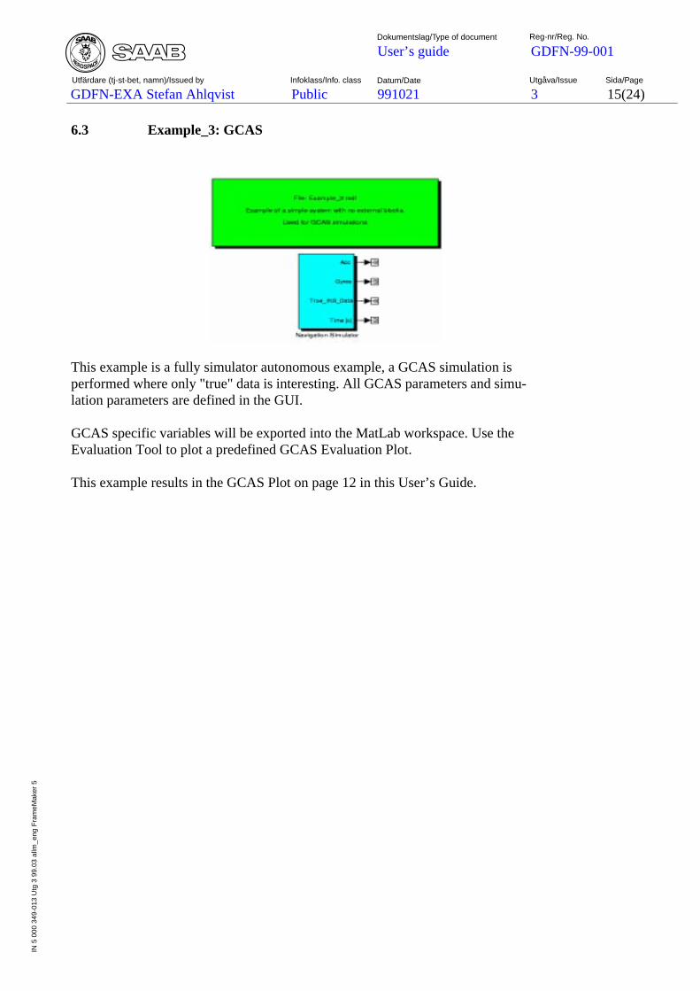
991021 3PublicGDFN-EXA Stefan Ahlqvist
User’s guide GDFN-99-001
Datum/Date Utgåva/Issue Sida/PageUtfärdare (tj-st-bet, namn)/Issued by
Dokumentslag/Type of document Reg-nr/Reg. No.
Infoklass/Info. class
15(24)
IN 5
000
349
-013
Utg
3 9
9.03
allm
_eng
Fra
meM
aker
5
6.3 Example_3: GCAS
This example is a fully simulator autonomous example, a GCAS simulation isperformed where only "true" data is interesting. All GCAS parameters and simu-lation parameters are defined in the GUI.
GCAS specific variables will be exported into the MatLab workspace. Use theEvaluation Tool to plot a predefined GCAS Evaluation Plot.
This example results in the GCAS Plot on page 12 in this User’s Guide.
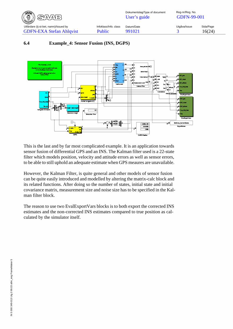
991021 3PublicGDFN-EXA Stefan Ahlqvist
User’s guide GDFN-99-001
Datum/Date Utgåva/Issue Sida/PageUtfärdare (tj-st-bet, namn)/Issued by
Dokumentslag/Type of document Reg-nr/Reg. No.
Infoklass/Info. class
16(24)
IN 5
000
349
-013
Utg
3 9
9.03
allm
_eng
Fra
meM
aker
5
6.4 Example_4: Sensor Fusion (INS, DGPS)
This is the last and by far most complicated example. It is an application towardssensor fusion of differential GPS and an INS. The Kalman filter used is a 22-statefilter which models position, velocity and attitude errors as well as sensor errors,to be able to still uphold an adequate estimate when GPS meaures are unavailable.
However, the Kalman Filter, is quite general and other models of sensor fusioncan be quite easily introduced and modelled by altering the matrix-calc block andits related functions. After doing so the number of states, initial state and initialcovariance matrix, measurement size and noise size has to be specified in the Kal-man filter block.
The reason to use two EvalExportVars blocks is to both export the corrected INSestimates and the non-corrected INS estimates compared to true position as cal-culated by the simulator itself.
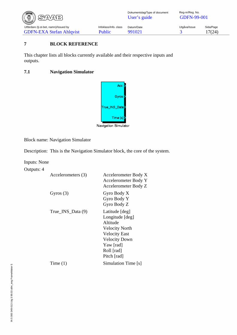
991021 3PublicGDFN-EXA Stefan Ahlqvist
User’s guide GDFN-99-001
Datum/Date Utgåva/Issue Sida/PageUtfärdare (tj-st-bet, namn)/Issued by
Dokumentslag/Type of document Reg-nr/Reg. No.
Infoklass/Info. class
17(24)
IN 5
000
349
-013
Utg
3 9
9.03
allm
_eng
Fra
meM
aker
5
7 BLOCK REFERENCE
This chapter lists all blocks currently available and their respective inputs andoutputs.
7.1 Navigation Simulator
Block name: Navigation Simulator
Description: This is the Navigation Simulator block, the core of the system.
Inputs: None
Outputs: 4Accelerometers (3) Accelerometer Body X
Accelerometer Body YAccelerometer Body Z
Gyros (3) Gyro Body XGyro Body YGyro Body Z
True_INS_Data (9) Latitude [deg]Longitude [deg]AltitudeVelocity NorthVelocity EastVelocity DownYaw [rad]Roll [rad]Pitch [rad]
Time (1) Simulation Time [s]
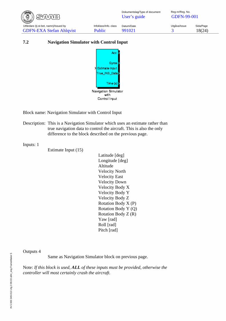
991021 3PublicGDFN-EXA Stefan Ahlqvist
User’s guide GDFN-99-001
Datum/Date Utgåva/Issue Sida/PageUtfärdare (tj-st-bet, namn)/Issued by
Dokumentslag/Type of document Reg-nr/Reg. No.
Infoklass/Info. class
18(24)
IN 5
000
349
-013
Utg
3 9
9.03
allm
_eng
Fra
meM
aker
5
7.2 Navigation Simulator with Control Input
Block name: Navigation Simulator with Control Input
Description: This is a Navigation Simulator which uses an estimate rather thantrue navigation data to control the aircraft. This is also the onlydifference to the block described on the previous page.
Inputs: 1Estimate Input (15)
Latitude [deg]Longitude [deg]AltitudeVelocity NorthVelocity EastVelocity DownVelocity Body XVelocity Body YVelocity Body ZRotation Body X (P)Rotation Body Y (Q)Rotation Body Z (R)Yaw [rad]Roll [rad]Pitch [rad]
Outputs 4Same as Navigation Simulator block on previous page.
Note:If this block is used,ALL of these inputs must be provided, otherwise thecontroller will most certainly crash the aircraft.
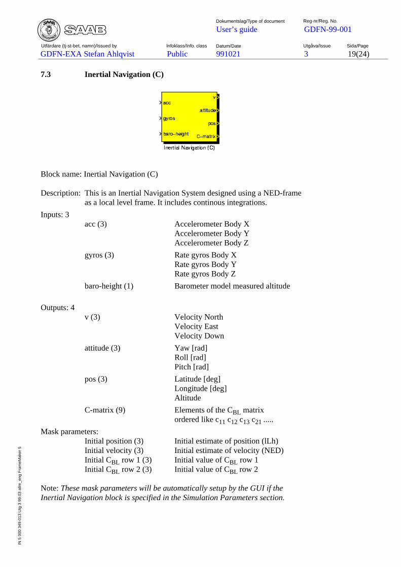
991021 3PublicGDFN-EXA Stefan Ahlqvist
User’s guide GDFN-99-001
Datum/Date Utgåva/Issue Sida/PageUtfärdare (tj-st-bet, namn)/Issued by
Dokumentslag/Type of document Reg-nr/Reg. No.
Infoklass/Info. class
19(24)
IN 5
000
349
-013
Utg
3 9
9.03
allm
_eng
Fra
meM
aker
5
7.3 Inertial Navigation (C)
Block name: Inertial Navigation (C)
Description: This is an Inertial Navigation System designed using a NED-frameas a local level frame. It includes continous integrations.
Inputs: 3acc (3) Accelerometer Body X
Accelerometer Body YAccelerometer Body Z
gyros (3) Rate gyros Body XRate gyros Body YRate gyros Body Z
baro-height (1) Barometer model measured altitude
Outputs: 4v (3) Velocity North
Velocity EastVelocity Down
attitude (3) Yaw [rad]Roll [rad]Pitch [rad]
pos (3) Latitude [deg]Longitude [deg]Altitude
C-matrix (9) Elements of the CBL matrixordered like c11 c12 c13 c21 .....
Mask parameters:Initial position (3) Initial estimate of position (lLh)Initial velocity (3) Initial estimate of velocity (NED)Initial CBL row 1 (3) Initial value of CBL row 1Initial CBL row 2 (3) Initial value of CBL row 2
Note:These mask parameters will be automatically setup by the GUI if theInertial Navigation block is specified in the Simulation Parameters section.
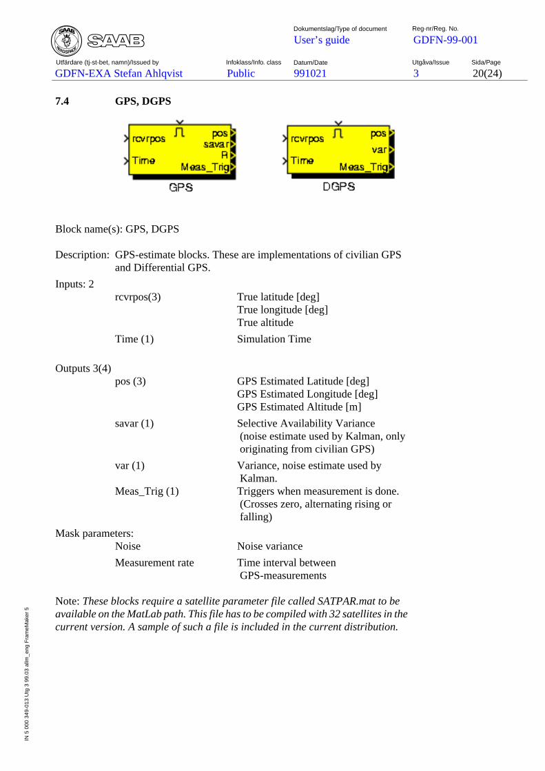
991021 3PublicGDFN-EXA Stefan Ahlqvist
User’s guide GDFN-99-001
Datum/Date Utgåva/Issue Sida/PageUtfärdare (tj-st-bet, namn)/Issued by
Dokumentslag/Type of document Reg-nr/Reg. No.
Infoklass/Info. class
20(24)
IN 5
000
349
-013
Utg
3 9
9.03
allm
_eng
Fra
meM
aker
5
7.4 GPS, DGPS
Block name(s): GPS, DGPS
Description: GPS-estimate blocks. These are implementations of civilian GPSand Differential GPS.
Inputs: 2rcvrpos(3) True latitude [deg]
True longitude [deg]True altitude
Time (1) Simulation Time
Outputs 3(4)pos (3) GPS Estimated Latitude [deg]
GPS Estimated Longitude [deg]GPS Estimated Altitude [m]
savar (1) Selective Availability Variance (noise estimate used by Kalman, only originating from civilian GPS)
var (1) Variance, noise estimate used by Kalman.
Meas_Trig (1) Triggers when measurement is done. (Crosses zero, alternating rising or falling)
Mask parameters:Noise Noise variance
Measurement rate Time interval between GPS-measurements
Note:These blocks require a satellite parameter file called SATPAR.mat to beavailable on the MatLab path. This file has to be compiled with 32 satellites in thecurrent version. A sample of such a file is included in the current distribution.

991021 3PublicGDFN-EXA Stefan Ahlqvist
User’s guide GDFN-99-001
Datum/Date Utgåva/Issue Sida/PageUtfärdare (tj-st-bet, namn)/Issued by
Dokumentslag/Type of document Reg-nr/Reg. No.
Infoklass/Info. class
21(24)
IN 5
000
349
-013
Utg
3 9
9.03
allm
_eng
Fra
meM
aker
5
7.5 EvalExportVars
Block name: EvalExportVars
Description: Block to be used, if Evaluation Tool is desired to be available at endof simulation.
Inputs: 5EST_pos (3) Estimated Latitude [deg]
Estimated Longitude [deg]Estimated Altitude
EST_vlocal (3) Estimated Velocity NorthEstimated Velocity EastEstimated Velocity Down
EST_attitude (3) Estimated Yaw [rad]Estimated Roll [rad]Estimated Pitch [rad]
True_INS_Data (9) To be directly connected to the Navigation Simulator
Time To be directly connected to the Navigation Simulator
Outputs: None
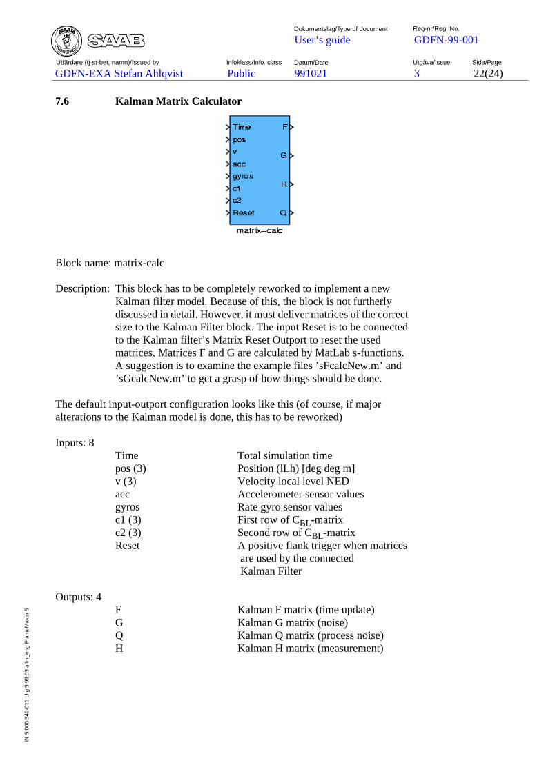
991021 3PublicGDFN-EXA Stefan Ahlqvist
User’s guide GDFN-99-001
Datum/Date Utgåva/Issue Sida/PageUtfärdare (tj-st-bet, namn)/Issued by
Dokumentslag/Type of document Reg-nr/Reg. No.
Infoklass/Info. class
22(24)
IN 5
000
349
-013
Utg
3 9
9.03
allm
_eng
Fra
meM
aker
5
7.6 Kalman Matrix Calculator
Block name: matrix-calc
Description: This block has to be completely reworked to implement a newKalman filter model. Because of this, the block is not furtherlydiscussed in detail. However, it must deliver matrices of the correctsize to the Kalman Filter block. The input Reset is to be connectedto the Kalman filter’s Matrix Reset Outport to reset the usedmatrices. Matrices F and G are calculated by MatLab s-functions.A suggestion is to examine the example files ’sFcalcNew.m’ and’sGcalcNew.m’ to get a grasp of how things should be done.
The default input-outport configuration looks like this (of course, if majoralterations to the Kalman model is done, this has to be reworked)
Inputs: 8Time Total simulation timepos (3) Position (lLh) [deg deg m]v (3) Velocity local level NEDacc Accelerometer sensor valuesgyros Rate gyro sensor valuesc1 (3) First row of CBL-matrixc2 (3) Second row of CBL-matrixReset A positive flank trigger when matrices
are used by the connected Kalman Filter
Outputs: 4F Kalman F matrix (time update)G Kalman G matrix (noise)Q Kalman Q matrix (process noise)H Kalman H matrix (measurement)

991021 3PublicGDFN-EXA Stefan Ahlqvist
User’s guide GDFN-99-001
Datum/Date Utgåva/Issue Sida/PageUtfärdare (tj-st-bet, namn)/Issued by
Dokumentslag/Type of document Reg-nr/Reg. No.
Infoklass/Info. class
23(24)
IN 5
000
349
-013
Utg
3 9
9.03
allm
_eng
Fra
meM
aker
5
7.7 Square Root Kalman Filter
Block name: Kalman Filter
This is a quite general implementation of a Square Root Kalman Filter. As param-eters state, measurement and noise sizes are input. Also initial states and initialcovariance matrix is input as mask parameters. The block uses Choleskyfactorization to calculate the Square Roots of the input matrices.
Inputs(7):F(s_size*s_size) Kalman F-matrixG(n_size*n_size) Kalman G-matrixH(m_size*s_size) Kalman H-matrixQ(s_size*n_size) Kalman Q-matrixR(m_size*m_size) Kalman R-matrixy(m_size) MeasurementMeasurement event(1) A trigger (rising or falling) to indicate
a new measurement on the y inport.
Outputs(4):New_Solution(1) A trigger to indicate a new Kalman
solutionMatrix Reset(1) A trigger to indicate reset of matricesInnov normed(s_size) Kalman Normed Innovationxhat(s_size) Kalman States
Mask Parameters:s_size State size Number of states in Kalman filterm_size Measurement size Size of the measurement vectorn_size Noise size Size of the process noise
Initial state Initial Kalman StateInitial covariance matrix Initial Kalman Covariance (P) matrixMax Interval update Specifies the maximum interval
between measurements before a time update is performed.
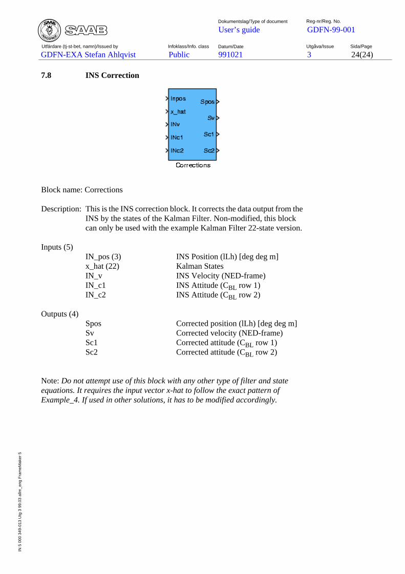
991021 3PublicGDFN-EXA Stefan Ahlqvist
User’s guide GDFN-99-001
Datum/Date Utgåva/Issue Sida/PageUtfärdare (tj-st-bet, namn)/Issued by
Dokumentslag/Type of document Reg-nr/Reg. No.
Infoklass/Info. class
24(24)
IN 5
000
349
-013
Utg
3 9
9.03
allm
_eng
Fra
meM
aker
5
7.8 INS Correction
Block name: Corrections
Description: This is the INS correction block. It corrects the data output from theINS by the states of the Kalman Filter. Non-modified, this blockcan only be used with the example Kalman Filter 22-state version.
Inputs (5)IN_pos (3) INS Position (lLh) [deg deg m]x_hat (22) Kalman StatesIN_v INS Velocity (NED-frame)IN_c1 INS Attitude (CBL row 1)IN_c2 INS Attitude (CBL row 2)
Outputs (4)Spos Corrected position (lLh) [deg deg m]Sv Corrected velocity (NED-frame)Sc1 Corrected attitude (CBL row 1)Sc2 Corrected attitude (CBL row 2)
Note:Do not attempt use of this block with any other type of filter and stateequations. It requires the input vector x-hat to follow the exact pattern ofExample_4. If used in other solutions, it has to be modified accordingly.