Union CollegeUnion | Digital Works

Honors Theses Student Work

6-2018

Development of a Fully Instrumented, ResonantTensegrity StrutKentaro Barhydt

Follow this and additional works at: https://digitalworks.union.edu/theses

Part of the Acoustics, Dynamics, and Controls Commons, Computer-Aided Engineering andDesign Commons, Computer and Systems Architecture Commons, Controls and Control TheoryCommons, Electrical and Electronics Commons, Electro-Mechanical Systems Commons, HardwareSystems Commons, and the Robotics Commons

This Open Access is brought to you for free and open access by the Student Work at Union | Digital Works. It has been accepted for inclusion in HonorsTheses by an authorized administrator of Union | Digital Works. For more information, please contact digitalworks@union.edu.

Recommended CitationBarhydt, Kentaro, "Development of a Fully Instrumented, Resonant Tensegrity Strut" (2018). Honors Theses. 1627.https://digitalworks.union.edu/theses/1627

Development of a Fully Instrumented, Resonant Tensegrity Strut

MER 498 – Report

03/13/2017 Student: Kentaro Barhydt

Advisor: Professor William Keat

I affirm that I have carried out all academic endeavors with full academic honesty

X______________________________________________________

Contents

Introduction & Background …………………………………………………………………… 1

Theoretical Models of a Single Tensegrity Strut ……………………………………………… 6

Implementation of Inertial Measurement Unit on Tensegrity Strut …………………………… 15

Design and Implementation of a Low-Frequency Vibration Motor …………………………… 21

Conclusions …………………………………………………………………………………… 31

References ……………………………………………………………………………………… 32

Appendices …………………………………………………………………………………… 33

1

Introduction & Background

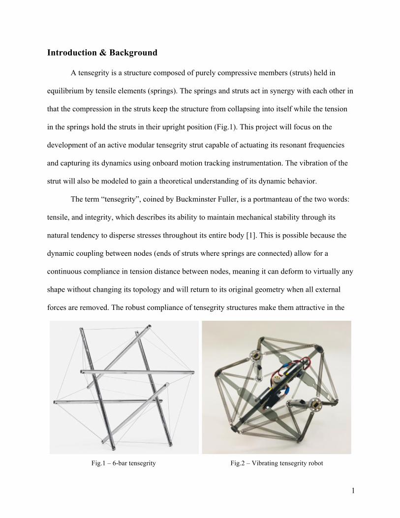
A tensegrity is a structure composed of purely compressive members (struts) held in

equilibrium by tensile elements (springs). The springs and struts act in synergy with each other in

that the compression in the struts keep the structure from collapsing into itself while the tension

in the springs hold the struts in their upright position (Fig.1). This project will focus on the

development of an active modular tensegrity strut capable of actuating its resonant frequencies

and capturing its dynamics using onboard motion tracking instrumentation. The vibration of the

strut will also be modeled to gain a theoretical understanding of its dynamic behavior.

The term “tensegrity”, coined by Buckminster Fuller, is a portmanteau of the two words:

tensile, and integrity, which describes its ability to maintain mechanical stability through its

natural tendency to disperse stresses throughout its entire body [1]. This is possible because the

dynamic coupling between nodes (ends of struts where springs are connected) allow for a

continuous compliance in tension distance between nodes, meaning it can deform to virtually any

shape without changing its topology and will return to its original geometry when all external

forces are removed. The robust compliance of tensegrity structures make them attractive in the

Fig.1 – 6-bar tensegrity Fig.2 – Vibrating tensegrity robot

2

field of soft robotics. The spring connections between struts absorb external forces and disperse

stress throughout its body, giving them a high strength-to-weight ratio and making them resilient

against impact forces that would cause traditional rigid robots to break. Tensegrities can adjust

the prestresses in its tensile connections as well, allowing it to deform under its own weight and

comply to different terrains. For these reasons, the NASA Ames Research Center is currently

developing a tensegrity-based robotic platform for planetary exploration, called SUPERball [2].

The current prototype locomotes by shifting its center of mass to achieve a rolling gait, which is

controlled by adjusting the prestress in its individual tensile connections. Its tensegrity-based

structure allows its gait to mechanically comply to different surfaces, making its ability to

traverse variable terrains more robust than previous planetary explorers. The high impact

resistance also enables high speed entry and landing without the use of airbags [3].

In addition to compliance, the deformation capabilities of tensegrity structures allow for a

greater range of complex dynamic motion than rigid structures. The dynamic coupling between

struts also allows for simplified actuation of complex motions that would otherwise require

multiple actuators using a rigid structure design. These characteristics parallel the robust

complexity of biomechanical locomotive systems found in animals and have caused tensegrities

to gain interest in the field of bioinspired robotics. Thomas Bliss et al. developed autonomous

control of a tensegrity-based swimmer that mimics a fishtail using Central Pattern Generators

(CPGs), which are systems of neurons found to control rhythmic motion responsible for

locomotion in animals, to achieve closed-loop entrainment to desired swimming gaits [4]. The

BEST Lab at University of California, Berkeley, has also developed a quadruped that utilizes a

tetrahedral tensegrity structure as a spine to support complex motions between the robot’s front

and rear legs, allowing for greater efficiency and stability in traversing irregular terrains [5].

3

Research at Union College lead by Professor John Rieffel has focused specifically on

exploiting the nonlinear complex dynamics of tensegrity structures. The tensegrities used are

designed to locomote through the vibration of the struts, which is evolved to achieve optimal

locomotion and control using genetic algorithms. These algorithms are based on the concept of

morphological communication. In, “Morphological Communication: Exploiting Coupled

Dynamics in a Complex Mechanical Structure to Achieve Locomotion”, Rieffel et al. presents

morphological communication as phenomena commonly found in nature in which dynamically

coupled physical systems act as neural networks capable of transferring signals through nodes

that can simultaneously actuate and sense other nodes [6]. This applies to the evolutionary

process in that the individual active (vibrating) struts are able to individually adapt their driving

frequency without direct communication with any of the other struts so that the gait of the entire

tensegrity structure evolves as a whole. The struts only have knowledge of their own dynamics,

and the forces applied by the springs affect those dynamics and act as feedback for the strut to

adjust to. This reduces the necessary computation significantly, allowing the tensegrity to bypass

the processing limitations of controlling its nonlinear coupled dynamics and take advantage of its

compliant properties and wide range of motion patterns.

Complex dynamic coupling is typically avoided in engineering design due to this

inability to control it through traditional means. Additionally, dynamic coupling is also typically

avoided to prevent resonance from occurring. This is because it can cause uncontrollable

increases in vibrational magnitude, which can be harmful to a rigid system’s operation and

structure. As a part of exploiting nonlinear dynamic coupling, Rieffel’s research hypothesizes

that optimal locomotion in vibrating tensegrities is achieved when driven at its resonant

frequencies due to the conservation of vibrational energy that causes the increase in amplitude.

4

This extends the implication that the natural frequencies, if known, should be utilized when

finding optimal gaits. The current version of the genetic algorithms only tracks the net motion of

the entire tensegrity robot and does not observe the dynamics of individual struts, making the

evolutionary process inefficient in that it cannot guide its genotype selection towards dynamic

behaviors known to correlate with optimal locomotion. Implementing methods of artificial

selection based on individual strut dynamics would significantly increase the efficiency of

evolution, therefore increasing the tensegrity’s ability to quickly adapt to variable environments.

Previous research has explored the dynamic response of tensegrity structures under

forced vibration. Oppenheim and Williams have demonstrated that the natural geometric

flexibility of tensegrities at equilibrium reduces the effect of natural damping in the tensile

elements, causing a longer rate of amplitude retention [7]. Bel Hadj Ali and Smith demonstrated

vibration control of a fixed, five-module tensegrity vertically actuated at one fixed node, and

determined that natural frequencies can be shifted away from excitation by adjusting prestress

levels [8]. Bohm and Zimmermann developed a symmetrical, single-actuated vibrating tensegrity

robot that could control the speed and direction of locomotion by adjusting prestress and driving

frequency respectively [9]. Bliss et al. developed and experimentally validated closed-loop

resonance entrainment of a linearly constrained biomimetic tensegrity swimmer to optimal

locomotive gaits using linear oscillators for cable actuation [10].

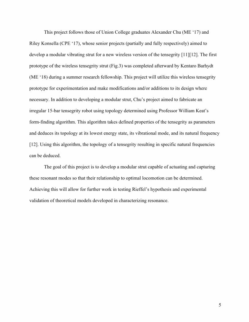
Fig.3 – Wireless modular strut for tensegrity robot

5

This project follows those of Union College graduates Alexander Chu (ME ‘17) and

Riley Konsella (CPE ‘17), whose senior projects (partially and fully respectively) aimed to

develop a modular vibrating strut for a new wireless version of the tensegrity [11][12]. The first

prototype of the wireless tensegrity strut (Fig.3) was completed afterward by Kentaro Barhydt

(ME ‘18) during a summer research fellowship. This project will utilize this wireless tensegrity

prototype for experimentation and make modifications and/or additions to its design where

necessary. In addition to developing a modular strut, Chu’s project aimed to fabricate an

irregular 15-bar tensegrity robot using topology determined using Professor William Keat’s

form-finding algorithm. This algorithm takes defined properties of the tensegrity as parameters

and deduces its topology at its lowest energy state, its vibrational mode, and its natural frequency

[12]. Using this algorithm, the topology of a tensegrity resulting in specific natural frequencies

can be deduced.

The goal of this project is to develop a modular strut capable of actuating and capturing

these resonant modes so that their relationship to optimal locomotion can be determined.

Achieving this will allow for further work in testing Rieffel’s hypothesis and experimental

validation of theoretical models developed in characterizing resonance.

6

2. Theoretical Models of a Single Tensegrity Strut

To properly characterize the dynamics of a multi-strut vibrating tensegrity, the dynamics

of a single strut must first be understood. Analyzing the behavior of an isolated strut provides the

insight necessary to analytically interpret experimental observations of the full tensegrity.

Therefore, the dynamics of an isolated single strut were first modeled using analytical and

numerical methods. In order to validate Keat’s small-angle linearity assumption used in the

predictive natural frequency algorithm, both a linear and nonlinear model were developed to

observe possible differences in their results given the same parameters. Having a computational

model also allowed for extensive parameter analysis, providing insight into how different

geometric constants and input variables affect the natural frequency of the strut.

2.1 Nonlinear Model

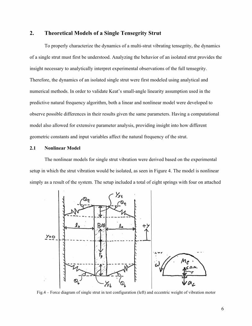
The nonlinear models for single strut vibration were derived based on the experimental

setup in which the strut vibration would be isolated, as seen in Figure 4. The model is nonlinear

simply as a result of the system. The setup included a total of eight springs with four on attached

Fig.4 – Force diagram of single strut in test configuration (left) and eccentric weight of vibration motor

7

to each end. Only the vertical displacement was observed and motion in other dimensions were

considered negligible because the strut movement along its axis was assumed to be dominant in

the particular tensegrity structure that the isolated spring geometry is based on. The lack of

actuation in the horizontal plane also implies that the spring configuration stays symmetric along

the axis of the strut at any given time, meaning the length and angle each spring is always equal

to all other springs connected to the same strut end. The motor speed was assumed to be

constant, as the electronic user input given to the tensegrity robot should translate directly

through to the mechanical input of the motor. If the voltage input and motor function do not have

a constant and direct relation, then experiments that rely on controlling frequency parameters,

like the genetic algorithm experiments conducted at Union College, could not properly

characterize the frequency response of the tensegrity as the input function would be accurately

represented. Since tensegrity structures are assumed to have negligible damping, the theoretical

models initially do not account for potential damping forces. The nonlinear model was first

derived as a second order differential equation as a function of time t with state variables of

vertical displacement y and acceleration ÿ:

ÿ = − $%&

𝑦 + ℎ* 𝑘 − ,-./0.

-123 435. 2

− $%&(𝑦 − ℎ*) 𝑘 − ,-./0.

-123(4/5.)2+ 8

%9𝑃4(𝑡) − 𝑔 (1)

where Py(t) denotes the vertical component of the centripetal force input of the motor:

𝑃4(𝑡) = 𝑀>𝑟𝜔A𝑠𝑖𝑛(𝜔𝑡) (2)

The first and second terms of the equation denote the top and bottom sets of springs respectively.

The variables and constants of both the nonlinear and linear equations are defined as:

𝑡 = time (s)

8

𝑦 = Vertical displacement of strut from y=0 (m) 𝑦& = Vertical distance between end of strut and respective spring mounting points (m) ℎE = 𝑦& @ y=0 (m) 𝜃 = Angle of spring from horizontal (rad) 𝑙H = Spring length @ θ=0° (rad) 𝑙E = Free length of spring (m) 𝑔 = Acceleration of gravity (m/s2) 𝐹4 = Vertical component of spring tension (N) 𝐹E = Initial tension in springs (N) 𝑀& = Mass of strut (Kg) 𝑀> = Mass of eccentric weight (Kg) 𝑟 = Centroidal radius of eccentric weight (m) 𝜔 = Motor speed (rad/s)

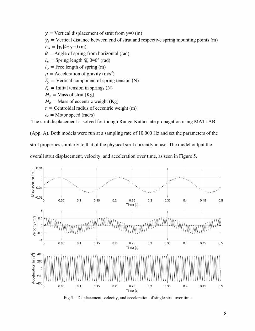
The strut displacement is solved for though Runge-Kutta state propagation using MATLAB

(App. A). Both models were run at a sampling rate of 10,000 Hz and set the parameters of the

strut properties similarly to that of the physical strut currently in use. The model output the

overall strut displacement, velocity, and acceleration over time, as seen in Figure 5.

Fig.5 – Displacement, velocity, and acceleration of single strut over time

9

2.2 Linear Model

The linear model was derived based on the same experimental setup used for the

nonlinear model with the exception that the assumption that the change in spring angle is small

enough to consider negligible, as seen in figure 6.

Fig.6 – Spring tension diagram of single spring for linear model. Small angle assumption assumes distance Y

is small enough to assume angle ⍺ is negligible. θ is constant.

This assumption resulted in the following equation for acceleration:

ÿ = − K%&

𝑘𝑠𝑖𝑛A𝜃 − L

-1235.2𝑐𝑜𝑠A𝜃 𝑦 + 8

%9𝑃4(𝑡) − 𝑔 (3)

where T denotes the tension in the springs when y = 0:

𝑇 = 𝑘 𝑙HA + ℎ*

A − 𝑙* + 𝐹* (4)

10

The spring constant term (multiple of y) could then be determined from this equation since θis

constant,makingtheentiretermconstant:

𝛴𝑘 = 𝑘𝑠𝑖𝑛A𝜃 − L

-1235.2𝑐𝑜𝑠A𝜃 (5)

Thiswasthenusedtoderivethenaturalfrequencyofthesystem,resultingin:

𝑓R =8AS

T,%9= 8

AS

,&UR2V/ W

X12YZ.

2[E&2V

%9 (6)

2.3 Results

The nonlinear and linear models generated fundamentally equal results and therefore

validated the small angle displacement assumption.

Fig.7 – Nonlinear model: vertical displacement of strut over time

11

Fig.8 – Linear model: vertical displacement of strut over time

As shown in figure 7 and 8, the function and periods of the frequency responses for both

models aligned with each other. Both plots reveal one overarching and one underlying sine wave

with frequencies of 10.6 Hz and 200 Hz respectively. The amplitude of the linear model is

slightly larger than that of the nonlinear model and there is an apparent phase shift of

approximately 20 degrees between them. However, both these discrepancies can be ignored for

the purposes of characterizing the strut dynamics because the function for both models are the

same and change proportionally as input frequency is adjusted. The frequency is crucial in that it

must stay consistently equal between the two models in order for the small angle displacement to

be valid. The frequency for both the nonlinear and linear responses aligned, therefore

theoretically confirming the assumption. A Fast Fourier Transform (FFT) was performed on the

numerical displacement results of the linear model, which confirmed the existence of two sine

waves and their respective frequencies (Fig. 9).

12

Fig. 10 – Fast Fourier Transform of linear displacement results

The natural frequency was calculated using (6) resulting in fn = 10.93 Hz, which aligned

with the overarching sine wave frequency found in both models with an error of 3.1%. When

tested at different motor speeds, the numerical and analytical natural frequency results stay

within a 3.5% to 4.5 % range of error with each other. While the significance of this error to

predicting natural frequencies will need to be determined experimentally, it is small and

consistent enough to conclude that the overarching sine wave present in the model results

represents the system’s natural frequency. The FFT also revealed a second sine wave with a

smaller amplitude than that of the overarching sine wave and a frequency of 200 Hz. This

frequency matched the driving frequency of the vibration motor and stayed within a ±0.005%

margin of error when tested at different motor speed inputs. From this correlation, it can be

concluded that the underlying sine wave present in the model results represents the driving

frequency of the strut. The identification of both the sine waves that comprise the vibration

response in context to the physical system theoretically confirms the validity of the linear model

13

in describing the strut dynamics. This in turn validates the use of the small angle displacement

assumption in Keat’s natural frequency algorithm.

A parameter analysis was conducted on the linear model to determine the limit and

magnitude of impact each independent parameter of the natural frequency equation (6). The

ranges of values analyzed for each parameter were estimated based on their reasonable upper

and/or lower limits for the current general tensegrity design.

Fig.11 – Natural frequency vs. strut mass, spring rate, spring angle at y = 0, and stretched spring length at y = 0

As seen in figure 11, the mass of the strut and the spring rate have the greatest impact on natural

frequency, although that impact diminishes logarithmically as their values increase. Spring rate

was shown to have the most consistent (although actually a root function) relationship with

natural frequency for the given range. The spring angle and stretched length at y = 0 were both

relatively inconsequential to the natural frequency.

2.4 Conclusions

The small-angle displacement assumption used in Keat’s predictive natural frequency

14

algorithm was successfully validated by developing and comparing linear and nonlinear models

of single strut vibration. Both models represent underlying frequencies of isolated strut motion

that aligned with the experimental setup as well. The mass of the strut and spring rate were also

determined to have a significant impact on the natural frequency of the system through a

parameter analysis, while the spring angle and stretched spring length were observed to be nearly

arbitrary.

15

3. Implementation of Inertial Measurement Unit on Tensegrity Strut

In order to empirically validate the theoretical models and observe phenomena such as

resonance, the dynamics of the tensegrity must be experimentally captured. Previous work using

the tensegrity for evolutionary algorithm testing only tracked the overall movement of the

tensegrity’s center of mass across a horizontal plane, which severely limited the understanding of

the mechanics behind what caused optimal locomotion. Therefore, the motion of each individual

strut must be captured in order to accurately observe its dynamic behavior. Given the constraints

of the tensegrity design and application, this must also be achieved while maintaining its wireless

control and small size.

3.1 Data Collection and Analysis

The necessary motion capture was achieved by implementing a 6-axis inertial

measurement unit (IMU) onto the strut. This method was chosen for its relatively high accuracy

and sampling rate, small size, and low cost. Other methods explored included visual tracking

using a high speed camera and spring tension measurement using load cells. Camera tracking is

ideal for the tensegrity design since it does not require any modification to the circuitry of the

strut. This method had previously been explored by Union College computer science students,

who tracked the position of a node (connection point between strut and springs) of the tensegrity

over time relative to the frame of the camera. However, this method was ruled out due to the

complexity needed to accurately track a tensegrity. Multiple cameras would be needed to track at

least six individual struts in three dimensions at a high enough resolution to accurately measure

position and a high enough frequency to accurately capture high frequencies (sampling rate must

be at least twice the highest frequency being observed). Camera tracking systems are sold

commercially explicitly for this purpose, but also cost hundreds of thousands of dollars.

16

Therefore, due to the complexity of tensegrity dynamics and the lack of equipment, camera

tracking was deemed an infeasible approach for this project.

The other method, using spring tension load cells, was also deemed infeasible due to the

lack of lightweight load cells available on the market. Since each spring would need at least one

load cell equipped to properly instrument the entire tensegrity, a 6-bar tensegrity would need

four load cells per strut (24 springs distributed between 6 struts), which would increase the total

weight by a very significant amount (lightest load cell found was 3.2 g, meaning 12.8g would be

added to the strut which weighs 60 g). The space taken up at the end of the struts would also

interfere with collisions with the ground during vibration, and the additional amp needed to

operate the cells would occupy even more space in the circuitry. An alternative exists in using

conductive rubber cord that changes its resistance as it stretches, allowing for its length to be

measured based on the current passing through it given a constant voltage. However, the

accuracy of this device does not meet the requirements of the project in that its specifications

provide a range of resistance per unit of length, and therefore was also ruled out as the best

potential motion capture method.

An IMU was integrated into the strut circuit to allow for onboard motion tracking. The

gyro/accelerometer used was a MPU-6050 module that can sense up to ±16 g at a resolution of

±2048 samples/g with six degrees of freedom: three-axis translation and three-axis rotation. The

MPU-6050 weighs ~1 g and has a maximum sampling rate of 1000Hz for translational

acceleration and 8000 Hz for rotational acceleration. Since oscillating motion must be recorded

at a sampling rate at least twice its frequency, the highest translational frequency that can be

captured is 500 Hz and the highest rotational acceleration that can be captured is 4000 Hz.

While the IMU is able to sample at 1000 Hz, Bluetooth connection to the strut was

17

unable to send samples to the user’s computer at the same rate. The maximum sampling rate

achievable by sending a live feed of samples over Bluetooth was approximately 7 Hz. Attempts

were made to increase the rate, such as minimizing the data sent per sample and communicating

between two Bluetooth modules instead of directly to the computer, but none could successfully

achieve a rate over 60 Hz. The minimum sampling rate requirement is approximately 400 Hz in

order to capture the higher frequencies obtainable by the vibration motor. The genetic algorithms

test a wide range of frequency inputs, so maintaining this range is important to finding optimal

locomotion in full tensegrity structures later in this project.

To increase the sampling rate to an adequate speed, onboard data storage was

implemented onto the strut using a microSD card and microSD shield module. This removed the

bottleneck of the slow Bluetooth communication and allowed the IMU to send data directly to

the microSD card through the microprocessor. The microSD shield connects to the plug-in pins

on the RFDuino, so the circuit was revised to avoid connecting other components to the pins

occupied by the shield. With this modification, the strut is now able to sample at a rate of 425

Hz, making proper data acquisition of high frequencies possible.

The program that runs the modular strut, written in Arduino (C/C++), also required

substantial revisions to allow for high sampling rate capabilities. The original code, written by

James Boggs and Riley Konsella, included a manual pulse width modulation (PWM) function

that allowed for digital control of the brushless motor speed. This method of motor control

needed to be replaced due to its use of a delay function in timing the output pulse, which stopped

all processes in the code for the specified amount of time. Since the total pulse period was set to

20 ms, the shortest possible amount of time elapsed between each sample was 20 ms, meaning

the sampling rate possible was 50 Hz. This issue was eliminated by programming the motor

18

control and data sampling to run in parallel instead of in series, which was accomplished in part

by the implementation of the updated brushed DC gearmotor (discussed further in section 4).

Although the Arduino code runs the modular strut, an interactive external python code is used to

control the strut by controlling the behavior of the Arduino code by restarting it and resetting its

parameters based on user input. Therefore, because the motor speed does not need to change

continuously over a gradient of values, the motor speed user input control was implemented in

the python code so that the internal behavior of the Arduino code can assume constant motor

speed throughout its runtime. This allowed the PWM function to be initialized and run until the

program is terminated, thus removing it from the loop in which data sampling is iteratively run.

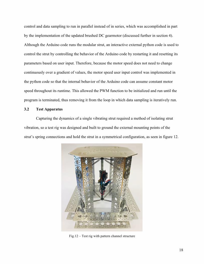
3.2 Test Apparatus

Capturing the dynamics of a single vibrating strut required a method of isolating strut

vibration, so a test rig was designed and built to ground the external mounting points of the

strut’s spring connections and hold the strut in a symmetrical configuration, as seen in figure 12.

Fig.12 – Test rig with pattern channel structure

19

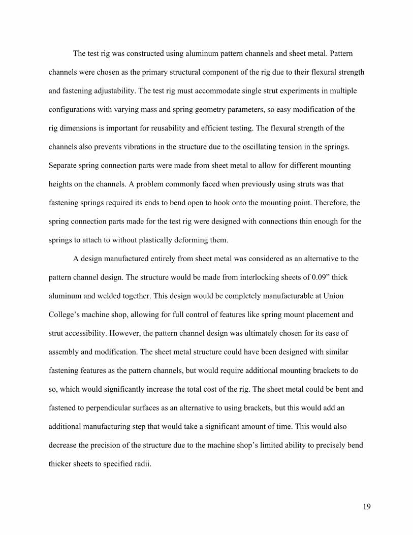
The test rig was constructed using aluminum pattern channels and sheet metal. Pattern

channels were chosen as the primary structural component of the rig due to their flexural strength

and fastening adjustability. The test rig must accommodate single strut experiments in multiple

configurations with varying mass and spring geometry parameters, so easy modification of the

rig dimensions is important for reusability and efficient testing. The flexural strength of the

channels also prevents vibrations in the structure due to the oscillating tension in the springs.

Separate spring connection parts were made from sheet metal to allow for different mounting

heights on the channels. A problem commonly faced when previously using struts was that

fastening springs required its ends to bend open to hook onto the mounting point. Therefore, the

spring connection parts made for the test rig were designed with connections thin enough for the

springs to attach to without plastically deforming them.

A design manufactured entirely from sheet metal was considered as an alternative to the

pattern channel design. The structure would be made from interlocking sheets of 0.09” thick

aluminum and welded together. This design would be completely manufacturable at Union

College’s machine shop, allowing for full control of features like spring mount placement and

strut accessibility. However, the pattern channel design was ultimately chosen for its ease of

assembly and modification. The sheet metal structure could have been designed with similar

fastening features as the pattern channels, but would require additional mounting brackets to do

so, which would significantly increase the total cost of the rig. The sheet metal could be bent and

fastened to perpendicular surfaces as an alternative to using brackets, but this would add an

additional manufacturing step that would take a significant amount of time. This would also

decrease the precision of the structure due to the machine shop’s limited ability to precisely bend

thicker sheets to specified radii.

20

3.4 Conclusions

Onboard motion tracking for individual struts was implemented into the modular strut

design using a IMU, allowing for translational and rotational acceleration measurement sampling

in three dimensions. Sampling data was collected onboard using microSD memory cards in order

to create a direct communication channel capable of processing high-frequency sampling data.

This system can consistently achieve a sampling rate of ~425 Hz, and its implementation did not

require any significant modifications to the physical design of the modular tensegrity strut. This

fast communication was developed alongside the new custom vibration motor, so experimental

results of this system are outlined in the following section.

21

4. Design and Implementation of a Low-Frequency Vibration Motor

The vibrating motor of the modular tensegrity strut needed to be redesigned in order for it

to drive the theoretical resonant frequencies of the 6-bar tensegrity as well as the current design

of the single strut. Using Keat’s model, the natural frequencies of a 6-bar tensegrity composed of

the modular tensegrity struts would have a number of resonant frequency combinations between

its active struts, all of which fall between 2 Hz and 17.6 Hz. The operating range of the brushless

motor from the previous design, 40 Hz to 230 Hz, does not encompass any of these frequencies.

Therefore, a custom motor was designed, manufactured, and implemented onto the strut to

achieve a lower frequency range that can actuate resonant frequencies, as well as increase overall

amplitude.

4.1 Vibration Motor Design

A gearmotor was chosen for the new motor design because the mechanical advantage of

the gearbox accomplished the exact purpose of the design renewal: given the same power input,

the gear motor increased the torque and decreased the rotational speed of the output shaft. The

inclusion of a gearbox was necessary since nearly all the motors researched either had too high

of a minimum driving frequency or too low of a stall torque. Achieving these results through

mechanical advantage instead of an alternative electronic design was necessary because the

power input could not increase without significantly increasing the weight of the strut and

requiring a redesigned battery mounting system.

The Pololu 10:1 Micro Metal Gearmotor LP 6V was chosen for the vibration motor

design for its operating frequency range of 0 Hz to 21.7 Hz. Although the maximum motor speed

is rated at free-run, the load torque resistance was assumed to be negligible compared to the

difference in the highest possible motor and resonant frequencies since the torque input is only

22

needed at high speeds to maintain the eccentric weight’s constant speed. Its rated voltage of 6V

is still lower than the 7.4V supply provided by the modular strut’s two LiPo batteries, making it

readily compatible with the current power configuration. The Pololu micro-gearmotor product

line also includes motor fastening accessories, meaning the motor can now be attached and

detached from the strut, unlike the previous friction-fit adhesive mount for the brushless motor.

Another crucial benefit of this specific motor was that it has a D-shaft output, meaning

attachments can be easily fastened and unfastened to and from it. This is important because a

custom eccentric mass was needed to reach the desired high vibrational amplitude at the low

resonant frequencies. The final eccentric weight design aimed to concentrate its mass as far from

the axis of rotation as possible, as seen in figure 13.

Fig.13 – Pololu 10:1 Micro Metal Gearmotor LP 6V equipped with custom eccentric weight

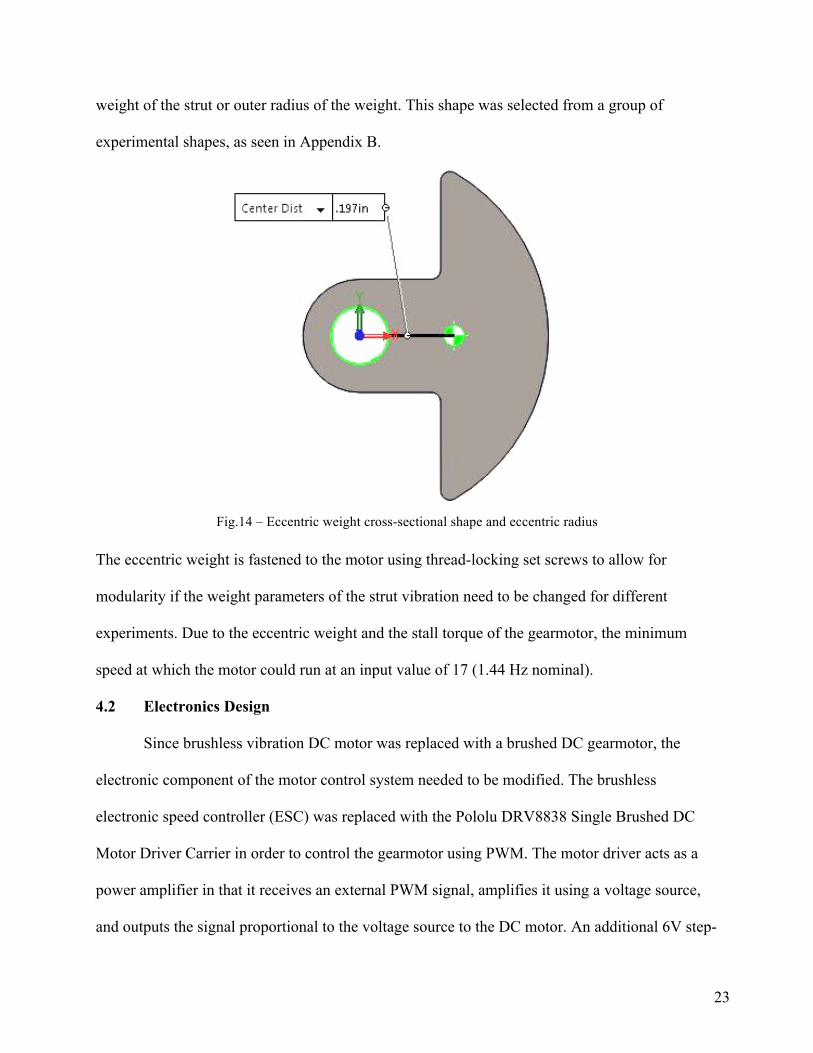
The weight was cut from a 5/16” thick 4140 hardened steel bar using a waterjet cutter and tapped

for a 3M set screw. The weight was cut in the “cut-off semicircle” shape, as seen in figure 14, in

order to maximize the eccentric radius while maintaining the same weight and thickness. This

was done in order to maximize centripetal force while avoiding any increase in the overall

23

weight of the strut or outer radius of the weight. This shape was selected from a group of

experimental shapes, as seen in Appendix B.

Fig.14 – Eccentric weight cross-sectional shape and eccentric radius

The eccentric weight is fastened to the motor using thread-locking set screws to allow for

modularity if the weight parameters of the strut vibration need to be changed for different

experiments. Due to the eccentric weight and the stall torque of the gearmotor, the minimum

speed at which the motor could run at an input value of 17 (1.44 Hz nominal).

4.2 Electronics Design

Since brushless vibration DC motor was replaced with a brushed DC gearmotor, the

electronic component of the motor control system needed to be modified. The brushless

electronic speed controller (ESC) was replaced with the Pololu DRV8838 Single Brushed DC

Motor Driver Carrier in order to control the gearmotor using PWM. The motor driver acts as a

power amplifier in that it receives an external PWM signal, amplifies it using a voltage source,

and outputs the signal proportional to the voltage source to the DC motor. An additional 6V step-

24

down voltage regulator was implemented to provide a constant 6V voltage supply to the motor

driver in order to avoid scaling inconsistencies when sending motor speed PWM signals. The

final circuit of the modular strut is shown in figure 15.

Fig.15 – Hand-drawn schematic of modular strut circuit and protoboard layout. Lines connecting dots denote

wire connections, and long rectangles with hatching marks denote copper tape.

With the electronic design updates and complete, the IMU motion capture system and

custom brushed gearmotor were integrated with the physical strut to make the latest version of

the fully instrumented, resonant tensegrity strut, as seen in figure 16.

Fig.16 – Latest prototype of fully instrumented, resonant tensegrity strut. Vertical chip is 3.3V step-up/step-down regulator used in previous design and is vertical due to lack of space on protoboard. Final prototype of

strut will use smaller 3.3V step-down regulator that will fit flat on protoboard. Batteries will also be secured in place using clips, similar to that of previous design, instead of using duct tape as shown in the picture.

25

4.3 Experimental Excitation of Single Strut Resonant Frequency

A series of tests were performed in which the instrumented strut was run at every

frequency input possible. These tests were run on a single strut using the pattern channel test rig.

The strut’s onboard Arduino code is programmed to take all two-digit hexadecimal values,

meaning it can take all numbers between 0 and 255. The tests were actually run starting at 15 and

ending on 249, meaning a total of 235 tests were run. These values convert to PWM output in

that a 0 input means the pulse is 100% off and the motor is stationary, and a 255 input means the

pulse is 100% on and the motor is at its fastest speed. A python code was written to run the strut

at a given speed for 30 seconds and then turn it off for another 30 seconds. This process would

be repeated for every frequency input between the user-defined upper and lower limits, with each

test increasing the input by one. The motion capture data from the IMU was appended to the

microSD card data file after each test.

The first attempt at running these tests failed due to the unexpectedly high amplitude the

strut vibrated at when excited at its resonant frequency. To accommodate for this, longer

channels were bought and a higher test rig was constructed. The two 150 mAh batteries lasted

throughout the entire testing session. The IMU collected a total of approximately 2.96 million

samples, which accumulated into a 48.6 Mb ASCII file. This size was too large for either

MATLAB or Excel to process without returning an error or crashing, so a script was written that

reads and separates this data into individual files for each test (App.A.5).

Before discussing the results of the tests, it should be noted that the theoretical models

were rendered partially inaccurate due to an invalid assumption. In their current state, the

theoretical models fail to account for continuous changes in motor speed due to the acceleration

it experiences from the vibration of the strut. This was determined to be significant as a result of

26

observing an unexpected phenomenon in the strut’s steady state vibration while testing, in that

when actuated near the system’s natural frequency, the oscillations of the motor and strut would

create a mode-locked loop and converge at the natural frequency. While this demonstrates an

interesting phenomenon that will be explored in future work, it also shows that the voltage input

from the user does not directly translate to the motor speed of the tensegrity strut. Since this

phenomenon is most likely due to the force of the strut acting on the eccentric weight, which

changes throughout its period, the motor speed cannot be assumed to be constant throughout its

period as well. Therefore, the function of the motor must be modeled as well for the theoretical

models to accurately characterize the entire system.

Despite this, the accuracy of the onboard motion capture system was confirmed and

resonance was still observed in the tensegrity strut. The experimental frequency response for

each test was observed and compared against high-speed video footage to confirm that the

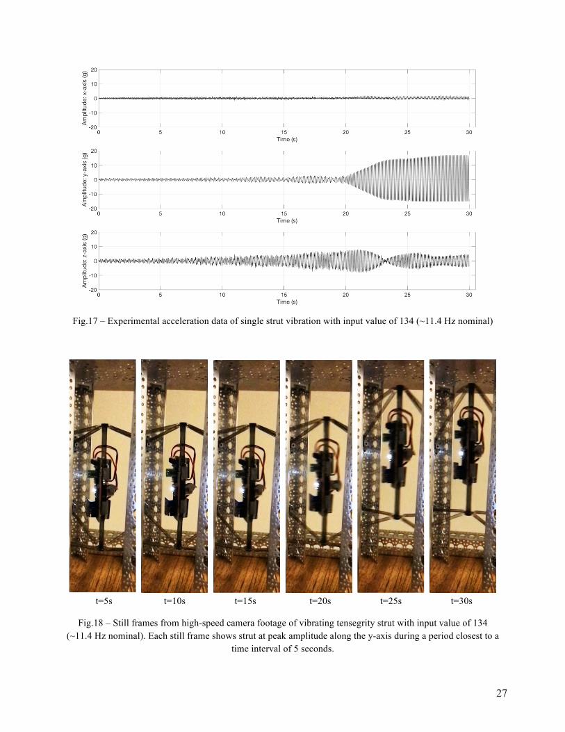
frequency and amplitude align. The IMU is mounted on the strut so that the x-axis of its local

orientation is parallel to the rotational axis of the vibration motor, and the y-axis is parallel to the

axis along the length of the strut. The experimental frequency response of the strut when run at

an input value of 134 (nominal frequency ~11.4 Hz) is shown in figure 17. Frequency locking

can be observed in this test through the change in frequency and amplitude. Between t=0s and

t=10s, the vibration is observed to have an approximate frequency of ~12 Hz and an amplitude of

±1 g, whereas once the vibration approaches steady state between t=27s and t=30s, the vibration

was observed to have an approximate frequency of ~9 Hz and an amplitude of ±16 g. These

results were compared against high-speed camera footage recorded at 240 FPS, as seen in figure

18.

27

Fig.17 – Experimental acceleration data of single strut vibration with input value of 134 (~11.4 Hz nominal)

t=5s t=10s t=15s t=20s t=25s t=30s

Fig.18 – Still frames from high-speed camera footage of vibrating tensegrity strut with input value of 134 (~11.4 Hz nominal). Each still frame shows strut at peak amplitude along the y-axis during a period closest to a

time interval of 5 seconds.

28

While the high speed footage was used to validate the overall behavior of the frequency

response, the precise acceleration measurement could not be confirmed due to a lack of scale in

the video. However, the resonance could still be observed without exact measurements of

acceleration, as the peaks in amplitude were observed on a scale relative to that of the other

frequency inputs. The experimental frequency measurement was confirmed by counting the

number of oscillations the strut experienced between a 5 second time interval when the strut

vibration was in steady state. This was then compared to the number of oscillations observed in

the measured data from the IMU.

The full frequency response of the strut vibration is visualized in figure 19. The

amplitude was measured from the steady state vibration of each test (App.A.6). From this

frequency response, the resonant frequency appears to lie between the input values 110 and 140.

However, due to the Frequency locking phenomenon, the resonant frequency most likely does

not lie

Fig.19 – Experimental frequency response of single strut vibration. Frequency domain is plotted as input

29

values for motor speed control due to indirect relationship between motor frequency and motor input voltage.

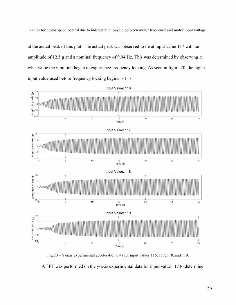
at the actual peak of this plot. The actual peak was observed to lie at input value 117 with an

amplitude of 12.5 g and a nominal frequency of 9.94 Hz. This was determined by observing at

what value the vibration began to experience frequency locking. As seen in figure 20, the highest

input value used before frequency locking begins is 117.

Input Value: 116

Input Value: 117

Input Value: 118

Input Value: 119

Fig.20 – Y-axis experimental acceleration data for input values 116, 117, 118, and 119.

A FFT was performed on the y-axis experimental data for input value 117 to determine

30

the experimental underlying frequency of the steady state strut vibration, as seen in figure 21.

The experimental resonant frequency was observed to be 9.67 Hz. When compared to the

Fig.19 – Experimental frequency response of single strut vibration. Frequency domain is plotted as input

values for motor speed control due to indirect relationship between motor frequency and motor input voltage.

frequency observed using the linear model (10.93 Hz), the theoretically natural frequency has a

calculated error of 13.03%.

31

5. Conclusions

The modular active wireless strut has been fully instrumented for onboard motion

tracking data collection and modified to actuate its resonant frequencies. Onboard acceleration

measurement with a sampling rate of 425 Hz was implemented using a 6-axis IMU. The

acceleration data was stored onboard as well using a microSD card. A custom vibration motor

was designed and manufactured using a brushed DC motor and a waterjet cut eccentric weight to

actuate the natural frequencies of the strut. The custom vibration motor has an operating range of

1.44 Hz to 21.7 Hz and can vibrate the strut at amplitudes of up to ±16 g.

Future work will focus on modifying the theoretical models to accommodate for

frequency locking. This will primarily involve modeling the motor speed as a function of the

strut acceleration as a feedback loop. Accounting for this will not only improve the accuracy of

the models but will also allow for a better understanding of how the coupled dynamics between

struts affect the vibration of struts individually. Further testing will also need to be conducted to

characterize the error of the linear and nonlinear models and the experimental range of in which

the IMU can properly capture amplitude and frequency.

32

References [1] Ingber , Donald E. . “The Architecture of Life .” Scientific American Jan 1998: 48-57. [2] A. P. Sabelhaus, J. Bruce, K. Caluwaerts, P. Manovi, R. F. Firoozi, S. Dobi, A. M.

Agogino, and V. Sunspiral, “System design and locomotion of SUPERball, an untethered tensegrity robot,” 2015 IEEE International Conference on Robotics and Automation (ICRA), Jul. 2015.

[3] J. Bruce, K. Caluwaerts, A. Iscen, A. P. Sabelhaus, and V. Sunspiral, “Design and evolution of a modular tensegrity robot platform,” 2014 IEEE International Conference on Robotics and Automation (ICRA), Sep. 2014.

[4] T. Bliss, T. Iwasaki, and H. Bart-Smith, “Central Pattern Generator Control of a Tensegrity Swimmer,” IEEE/ASME Transactions on Mechatronics, vol. 18, no. 2, pp. 586–597, 2013.

[5] A. P. Sabelhaus, H. Ji, P. Hylton, Y. Madaan, C. Yang, A. M. Agogino, J. Friesen, and V. Sunspiral, “Mechanism Design and Simulation of the ULTRA Spine: A Tensegrity Robot,” Volume 5A: 39th Mechanisms and Robotics Conference, 2015.

[6] Rieffel, J. , Valero-Cuevas, F. and Lipson, H. (2010) "Morphological Communication: Exploiting Coupled Dynamics in a Complex Mechanical Structure to Achieve Locomotion". J. R. Soc. Interface.

[7] I. J. Oppenheim, “Vibration of an Elastic Tensegrity Structure,” European Journal of Mechanics, vol. 20, 2001.

[8] N. Bel Hadj Ali, “Dynamic Behavior and Vibration Control of a Tensegrity Structure,” International Journal of Solids and Structures, vol. 47, no. 9, pp. 1285–1296, 2010.

[9] V. Bohm and K. Zimmermann, “Vibration-driven mobile robots based on single actuated tensegrity structures,” 2013 IEEE International Conference on Robotics and Automation, 2013.

[10] T. Bliss, J. Werly, T. Iwasaki, and H. Bart-Smith, “Experimental Validation of Robust Resonance Entrainment for CPG-Controlled Tensegrity Structures,” IEEE Transactions on Control Systems Technology, vol. 21, no. 3, pp. 666–678, Mar. 2012.

[11] R. Konsella, “Designing a Modular Strut for Union’s Tensegrity Robot,” thesis, 2017. [12] A. Chu, “Through Yonder Window Breaks: The Rise of JULIET,” thesis, 2017 [13] J. Rieffel, W. Keat, B. Humphreys, M. Khazanov. “Exploiting Dynamical Complexity in

A Physical Tensegrity Robot to Achieve Locomotion.” Advances in Artificial Life 12 (2013)

33

Appendix A.1: Vibration Model MATLAB Code – Nonlinear StrutVibrationModelNonlinear.m

% Single VVValtr Strut Vibration % Linear Model clear all global g Me Ms r omega k l0 lx F0 h0 g = 9.81; % m/s^2 Me = 0.005; % kg Ms = 0.056; % kg r = 4 * 0.0058 / (3 * pi()); % m omega = 2 * pi() * 5000 / 60; %rad/s k = 0.19 * 175.196945; % N/m l0 = 2.47 * 0.0254; % m lx = 3 * 0.0254; % m F0 = 0.4 * 4.45; % N h0 = 0.05; % m % Define time step and sampling range deltat = 0.001; % s startTime = 0; % s endTime = 100; % s t = [startTime:deltat:endTime]; % Calculate Ysag Ysag = findYsag(); % Initialize state vector yInit = [Ysag;0]; y = yInit; % Conduct state propogation using Runge Kutta method for i = 1:length(t)-1 ydot(:,i) = accelerationFunction(y(:,i),t(i)); k1 = ydot(:,i); k2 = accelerationFunction(y(:,i) + (deltat/2)*k1,t(i)); k3 = accelerationFunction(y(:,i) + (deltat/2)*k2,t(i)); k4 = accelerationFunction(y(:,i) + deltat*k3,t(i)); y(:,i+1) = y(:,i) + (deltat/6)*(k1 + 2*k2 + 2*k3 + k4); end Yfft = fft(y(1,:)); Yfft_mag = abs(Yfft)/length(Yfft); % Calculate state derivative at last time sample ydot(:,length(t)) = accelerationFunction(y(:,length(t)-1),t(i)); % Plot displacement figure('name','Nonlinear Model - Displacement','units',... 'normalized','position',[0,0.5,0.5,0.5]) plot(t,y(1,:),'k','LineWidth', 1.5) set(gca, 'FontSize', 20) set(gca,'YTick',(-1:0.002:1)) xlabel('Time (s)','FontSize',22)

34

ylabel('Displacement (m)','FontSize',22) xlim([max(0,endTime-1),endTime]) ylim([-0.014,0.004]) grid on % Plot FFT results binDomain = 1:length(Yfft_mag); freqDomain = binDomain*(1/endTime); figure('name','Magnitude vs Frequency FFT results - Linear','units',... 'normalize','position',[0.5,0.5,0.5,0.5]) plot(freqDomain,Yfft_mag) xlabel('bins','FontSize',22) ylabel('Amplitude','FontSize',22) xlim([0,freqDomain(end)/2]) set(gca, 'FontSize', 20) % Plot velocity figure('name','Velocity of Cart Along Surface Over Time','units',... 'normalized','position',[0,0,1,1]) plot(t,y(2,:)) set(gca, 'FontSize', 14) xlabel('Time (s)','FontSize',16) ylabel('Velocity (m/s)','FontSize',16) grid on % Plot acceleration figure('name','Acceleration of Cart Along Surface Over Time','units',... 'normalized','position',[0,0,1,1]) plot(t,ydot(2,:)) set(gca, 'FontSize', 14) xlabel('Time (s)','FontSize',16) ylabel('Acceleration (m/s^2)','FontSize',16) grid on % Plot displacement, velocity, and acceleration together figure('name','Displacement, Velocity, and Acceleration Over Time',... 'units','normalized','position',[0,0,1,1]) subplot(3,1,1) plot(t,y(1,:)) set(gca, 'FontSize', 14) xlabel('Time (s)','FontSize',16) ylabel('Displacement (m)','FontSize',16) grid on subplot(3,1,2) plot(t,y(2,:)) set(gca, 'FontSize', 14) xlabel('Time (s)','FontSize',16) ylabel('Velocity (m/s)','FontSize',16) grid on subplot(3,1,3) plot(t,ydot(2,:)) set(gca, 'FontSize', 14) xlabel('Time (s)','FontSize',16) ylabel('Acceleration (m/s^2)','FontSize',16) grid on

35

accelerationFunction.m

function ydot = accelerationFunction(y,t) global g Me Ms r omega k l0 lx F0 h0 ydot1 = y(2); ydot2 = -(4/Ms)*(y(1)+h0)*(k-((k*l0-F0)/sqrt(lx^2+(y(1)+h0)^2)))... -(4/Ms)*(y(1)-h0)*(k-((k*l0-F0)/sqrt(lx^2+(y(1)-h0)^2)))... -g+(Me/Ms)*r*omega^2*sin(omega*t); ydot = [ydot1;ydot2]; end

findYsag.m

function ysag = findYsag() global g Ms k l0 lx F0 h0 lmax = l0 + 3.200; ymax = sqrt(lmax^2 - lx^2) - h0; for y = -ymax:0.0000001:ymax Fsum = -4*(y+h0)*(k-((k*l0-F0)/sqrt(lx^2+(y+h0)^2)))-4*(y-h0)*... (k-((k*l0-F0)/sqrt(lx^2+(y-h0)^2))); sum = Fsum-Ms*g; if sum <= 0.0001 && sum >= -0.0001 ysag = y; % disp(sum); % disp(y) end end end

36

Appendix A.2: Vibration Model MATLAB Code – Linear StrutVibrationModelLinear.m

% Single VVValtr Strut Vibration % Linear Model clear all global g Me Ms r omega k l0 lx F0 h0 ysag L T theta g = 9.81; % m/s^2 Me = 0.005; % kg Ms = 0.056; % kg r = 4 * 0.0058 / (3 * pi()); % m omega = 2 * pi() * 12000 / 60; %rad/s k = 0.19 * 175.196945; % N/m l0 = 2.47 * 0.0254; % m lx = 3 * 0.0254; % m F0 = 0.4 * 4.45; % N h0 = 0.05; % m ysag = findYsag(); % m L=(lx^2+h0^2)^0.5; T=k*(L - l0) + F0; theta=atand(h0/lx); % Define time step and sampling range deltat = 0.001; % s startTime = 0; % s endTime = 100; % s t = [startTime:deltat:endTime]; % Initialize state vector y2Init = [0;0]; y2 = y2Init; % Conduct state propogation using Runge Kutta method for j = 1:length(t)-1 y2dot(:,j) = accelerationFunction_v5(y2(:,j),t(j)); k1 = y2dot(:,j); k2 = accelerationFunction_v5(y2(:,j) + (deltat/2)*k1,t(j)); k3 = accelerationFunction_v5(y2(:,j) + (deltat/2)*k2,t(j)); k4 = accelerationFunction_v5(y2(:,j) + deltat*k3,t(j)); y2(:,j+1) = y2(:,j) + (deltat/6)*(k1 + 2*k2 + 2*k3 + k4); end % Calculate state derivative at last time sample y2dot(:,length(t)) = accelerationFunction_v5(y2(:,length(t)-1),t(j)); % Fast Fourier Transform Yfft = fft(y2(1,:)); Yfft_mag = abs(Yfft)/length(Yfft); % Plot displacement2 figure('name','Linear Model - Displacement','units',... 'normalized','position',[0,0,0.5,0.5]) plot(t,y2(1,:),'k','LineWidth', 1.5) set(gca, 'FontSize', 20)

37

set(gca,'YTick',(-1:0.002:1)) xlabel('Time (s)','FontSize',22) ylabel('Displacement (m)','FontSize',22) xlim([max(0,endTime-1),endTime]) ylim([-0.014,0.004]) grid on % Plot FFT results binDomain = 1:length(Yfft_mag); freqDomain = binDomain*(1/endTime); figure('name','Magnitude vs Frequency FFT results - Linear','units',... 'normalize','position',[0.5,0,0.5,0.5]) plot(freqDomain,Yfft_mag) xlabel('bins','FontSize',22) % understand how to convert to Hz ylabel('Amplitude','FontSize',22) % find out units of amplitude xlim([0,freqDomain(end)/2]) set(gca, 'FontSize', 20)

accelerationFunction_v5.m

function ydot = accelerationFunction_v5(y,t) global g Me Ms r omega k L T theta fsum2=-8*(k*sind(theta)*y(1)*sind(theta)... + T/L*cosd(theta)*y(1)*cosd(theta)); ydot1 = y(2); ydot2 = (1/Ms)*fsum2-g+(Me/Ms)*r*omega^2*sin(omega*t); ydot = [ydot1;ydot2]; end

38

Appendix A.3: Natural Frequency Parameter Analysis NatrualFrequencyParameterAnalysis.m

% Single VVValtr Strut Vibration % Natural Frequency Parameter Analysis % Linear Model clear all close all % Motor Frequency omega = 2 * pi() * 12000 / 60; % rad/s drivingFreq = omega/(2 * pi()); % Hz % ------------------------------------------------------------------------ % DEFAULT CALCULATIONS % Input parameters Ms = 0.0572; % Kg k = 0.19 * 175.196945; % N/m l0 = 2.47 * 0.0254; % m lx = 3 * 0.0254; % m F0 = 0.4 * 4.45; % N * NO INITIAL TENSION DATA FOR MCMASTER SPRINGS* h0 = 0.02; % m % Dependent parameters L=(lx^2+h0^2)^0.5; % m T=k*(L - l0) + F0; % N theta=atand(h0/lx); % deg % Natrual frequency calculation naturalFreq = sqrt(8*(k*sin(theta)^2+(T/L)*cos(theta)^2)/Ms)/(2*pi); % ------------------------------------------------------------------------ % VARIABLE MASS % Variable range MsRange = [0.05:0.001:0.5]; % Kg naturalFreqMs = []; for i = 1:length(MsRange) MsVar = MsRange(i); naturalFreqMs(i) = sqrt(8*(k*sind(theta)^2+... (T/L)*cosd(theta)^2)/MsVar)/(2*pi); end figure('name','VARIABLE MASS','units',... 'normalized','position',[0,0,1,1]) subplot(2,2,1) plot(MsRange,naturalFreqMs,'k') set(gca, 'FontSize', 14) xlabel('Strut Mass (Kg)','FontSize',16) ylabel('Natural Frequency (Hz)','FontSize',16) % ylim([0,60]) grid on

39

% ------------------------------------------------------------------------ % VARIABLE SPRING RATE % Variable range kRange = [0:300]; % N/m naturalFreqK = []; for i = 1:length(kRange) kVar = kRange(i); TVar = kVar*(L - l0) + F0; naturalFreqK(i) = sqrt(8*(kVar*sind(theta)^2+... (TVar/L)*cosd(theta)^2)/Ms)/(2*pi); end % figure('name','VARIABLE SPRING RATE','units',... % 'normalized','position',[0,0,1,1]) subplot(2,2,2) plot(kRange,naturalFreqK,'k') set(gca, 'FontSize', 14) xlabel('Spring Rate (N/m)','FontSize',16) ylabel('Natural Frequency (Hz)','FontSize',16) % ylim([0,60]) grid on % ------------------------------------------------------------------------ % VARIABLE ANGLE % Variable range thetaRange = [0:0.1:90]; % deg naturalFreqTheta = []; for i = 1:length(thetaRange) thetaVar = thetaRange(i); naturalFreqTheta(i) = sqrt(8*(k*sind(thetaVar)^2+... (T/L)*cosd(thetaVar)^2)/Ms)/(2*pi); end % figure('name','VARIABLE ANGLE','units',... % 'normalized','position',[0,0,1,1]) subplot(2,2,3) plot(thetaRange,naturalFreqTheta,'k') set(gca, 'FontSize', 14) xlabel('Spring Angle at y=0 (deg)','FontSize',16) ylabel('Natural Frequency (Hz)','FontSize',16) xlim([0,90]) % ylim([0,60]) grid on % ------------------------------------------------------------------------ % VARIABLE STRECHED LENGTH % Variable range LRange = [l0:0.001:0.25]; % m naturalFreqL = []; for i = 1:length(LRange) LVar = LRange(i); TVar = k*(LVar - l0) + F0;

40

naturalFreqL(i) = sqrt(8*(k*sind(theta)^2+... (TVar/LVar)*cosd(theta)^2)/Ms)/(2*pi); end % figure('name','VARIABLE STRECHED LENGTH','units',... % 'normalized','position',[0,0,1,1]) subplot(2,2,4) plot(LRange,naturalFreqL,'k') set(gca, 'FontSize', 14) xlabel('Stretched Spring Length at y=0 (m)','FontSize',16) ylabel('Natural Frequency (Hz)','FontSize',16) xlim([l0,0.25]) % ylim([0,60]) grid on % ------------------------------------------------------------------------ % VARIABLE INITIAL TENSION % Variable range F0Range = [0:0.01:1]; % N naturalFreqF0 = []; for i = 1:length(F0Range) F0Var = F0Range(i); TVar = k*(L - l0) + F0Var; naturalFreqF0(i) = sqrt(8*(k*sin(theta)^2+... (TVar/L)*cos(theta)^2)/Ms)/(2*pi); end % figure('name','VARIABLE INITIAL TENSION','units',... % 'normalized','position',[0,0,1,1]) % subplot(3,2,5) % plot(F0Range,naturalFreqF0,'k') % set(gca, 'FontSize', 14) % xlabel('Spring Tension (N)','FontSize',16) % ylabel('Natural Frequency (Hz)','FontSize',16) % % ylim([0,60]) % grid on

41

Appendix A.4: Experimental Data Frequency Analysis MATLAB Code ExpFreqAnalysis.m

% Experimental Vibration Frequency Analysis % NOTES: % - SMOOTH ALL DATA AT BEGINNING SINCE MOST ACCURATE AMP DATA CAN BE % CALCULATED WITH IT, GIVEN PROPER ORDER AND WINDOW SIZE VALUES ARE % USED,AND IT DOESN'T EFFECT CALCULATED FREQUENCY clc clear all close all % ------------------------------------------------------------------------ % PARAMETER SETTINGS runtime = 30.001; % s acclRange = 16; % +/-[2,4,8,16] g % gyroRange = 250; % +/-[250,500,1000,2000] dps ststStartTime = 16; % observed start time for st-st in s % ------------------------------------------------------------------------ % LOAD TEST DATA AS ARRAY data = load('test_d022618_t0248am_s130.txt'); % SINE WAVE BASED ON THIS % data = load('test_d022618_t0248am_s130.txt'); % sp40_t30 = csvread('sp40_t30.csv'); % ISOLATE DOF ax = data(:,1); ay = data(:,2); az = data(:,3); % gx = data(:,1); % gy = data(:,2); % gz = data(:,3); % CONVERT DOF VECTORS ax = ax .* (acclRange/32768); ay = ay .* (acclRange/32768); az = az .* (acclRange/32768); % gx = gx .* (gyroRange/32768); % gy = gy .* (gyroRange/32768); % gz = gz .* (gyroRange/32768); % ADJUST ZERO REFERENCE FOR CALIBRATION ax = ax - ax(1); ay = ay - ay(1); az = az - az(1); % gx = gx - gx(1); % gy = gy - gy(1); % gz = gz - gz(1); % ------------------------------------------------------------------------ % DEPENDENT PARAMETERS

42

samples = length(ax(:,1)); deltat = runtime/samples; t = 0:deltat:runtime-deltat; rate = samples/runtime; ststStartSample = ceil(ststStartTime*rate); % start sample for st-st in s % ------------------------------------------------------------------------ % FFT ayFFT = fft(ay(ststStartSample:end)); % FFT of steady state region ayFFT = abs(ayFFT); % convert FFT to magnitude spectrum ayFFT = 2 .* ayFFT ./ length(ayFFT); % scale FFT to amplitude units freqDomain = (0:length(ayFFT)-1) .* rate ./ length(ayFFT); % plot(ay(ststStartSample:end)); % plot(ayFFT); % DOMINANT SINE WAVE [ayDomAmp,ayDomBin] = max(ayFFT); ayDomFreq = freqDomain(ayDomBin); disp(freqDomain(ayDomBin)); % ayDomWave = ayDomAmp * sin(2 * pi() * ayDomFreq .* t); ayDomWave = max(ay) * sin(2 * pi() * ayDomFreq .* t); % ------------------------------------------------------------------------ % SMOOTHED WAVE DATA % **larger window will cause more smoothing but greater amplitude decrease axSmth = sgolayfilt(ax,3,7); aySmth = sgolayfilt(ay,3,7); azSmth = sgolayfilt(az,3,7); % AVE SMOOTHED AMPLITUDE & FREQUENCY peaks = findpeaks(aySmth((ststStartSample:end))); peaks = peaks(peaks > 0); aySmthAmp = mean(peaks); aySmthFreq = length(peaks) / (runtime - deltat - ststStartTime); disp(aySmthFreq); % temp testing of fft on smoothed data to find freq aySmthFFT = fft(aySmth(ststStartSample:end)); aySmthFFT = abs(aySmthFFT); aySmthFFT = 2 .* aySmthFFT ./ length(aySmthFFT); freqDomainSmth = (0:length(aySmthFFT)-1) .* rate ./ length(aySmthFFT); [aySmthDomAmp,aySmthDomBin] = max(aySmthFFT); aySmthDomFreq = freqDomainSmth(aySmthDomBin); disp(freqDomainSmth(aySmthDomBin)); % ------------------------------------------------------------------------ % PLOT FFT figure('name','FFT Acceleration: y-axis','units','normalized',... 'position',[0,0,1,1]) plot(freqDomain,ayFFT) xlim([0,rate/2]) % PLOT ACCL GRAPHS figure('name','Acceleration Experimental Data','units','normalized',...

43

'position',[0,0,1,1]) subplot(3,1,1) plot(t,ax,'k'); hold on % plot(t,axSmth,'k'); xlim([0,30.5]) ylim([-20,20]) xlabel('Time (s)','FontSize',16) ylabel('Amplitude: x-axis (g)','FontSize',18) set(gca, 'FontSize', 16) grid on subplot(3,1,2) plot(t,ay,'k'); hold on % plot(t,aySmth,'k'); % plot(t(ststStartSample:end),ayDomWave(ststStartSample:end),'--'); xlim([0,30.5]) ylim([-20,20]) xlabel('Time (s)','FontSize',16) ylabel('Amplitude: y-axis (g)','FontSize',18) set(gca, 'FontSize', 16) grid on subplot(3,1,3) plot(t,az,'k'); hold on % plot(t,azSmth,'k'); xlim([0,30.5]) ylim([-20,20]) xlabel('Time (s)','FontSize',16) ylabel('Amplitude: z-axis (g)','FontSize',18) set(gca, 'FontSize', 16) grid on figure('name','Y-axis Close Up Acceleration','units','normalized',... 'position',[0,0,0.6,0.6]) plot(t,ay,'k'); xlim([20,21]) ylim([-20,20]) xlabel('Time (s)','FontSize',16) ylabel('Amplitude: y-axis (g)','FontSize',18) set(gca, 'FontSize', 16) grid on

get_freq_exp.m

function freq_exp = get_freq_exp(data, runTime) % This function determines the frequency of experimental sine wave data. % Only works for simple waves. % NOTE: Only enter range of data after oscillation starts and before % amplitude becomes effected by noise. % NOTE: Data must have at least five oscillations. % % file_var: name of variable loaded from ASCII file % time_col: column in file_var containing time data

44

% data_col: column in file_var containing desired position data % start_time: start time for peak count % end_time: end time for peak count first_peak = 1; while data(first_peak + 1) <= data(first_peak) first_peak = first_peak + 1; end while data(first_peak + 1) >= data(first_peak) first_peak = first_peak + 1; end last_peak = length(data); while data(last_peak - 1) <= data(last_peak) last_peak = last_peak - 1; end while data(last_peak - 1) >= data(last_peak) last_peak = last_peak - 1; end peak_count = 0; % number of peaks observed initialized to 0 increasing = 0; % initialize increasing as false % Last peak is counted, first peak is not for i = first_peak:last_peak + 1 % check if function is increasing if increasing == 1 % check if sample position value decreased if data(i) < data(i-1) % add to peak count peak_count = peak_count + 1; increasing = 0; % set increasing as false end elseif increasing == 0 % check if sample position value increased if data(i) > data(i-1) increasing = 1; % set increasing as true end end end sRate = length(data)/runtime; %calculate average frequency freq_exp = (peak_count / (last_peak - first_peak)) * sRate; end

45

Appendix A.5: Experimental Data File Separator expDataSplitter.m

% Data File Splitter % Only works with .txt files clear all delimiter = 999999999; startTimeCol = 1; endTimeCol = 2; speedValueCol = 3; dataAllFileName = 'test_d022618_t0248am_s121_s249.txt'; dataAll = load(dataAllFileName); [path,dataAllFileName,extension] = fileparts(dataAllFileName); %#ok<ASGLU> clear path extension if exist(dataAllFileName) ~= 7 mkdir(dataAllFileName) end c = 1; nameChanged = false; while nameChanged == false c = c + 1; if dataAllFileName(c:c+1) == '_s' fileName = dataAllFileName(1:c+1); nameChanged = true; end end prevTestDlmRow = 1; for i = 1:length(dataAll) if dataAll(i,:) == [delimiter,delimiter,delimiter] testSpeed = dataAll(i-1,3); fileNameS = char(fileName+string(testSpeed)); dlmwrite(fileNameS,dataAll(prevTestDlmRow:i-1,:)) movefile(fileNameS,dataAllFileName) prevTestDlmRow = i+1; end end

46

Appendix A.6: Experimental Frequency Response Plot Script frequencyResponce.m

% Frequency Responce Plot clear all close all maxMotorSpeed = 1300; % RPM massFileFolder1 = 'test_d022518_t1223am_s15_s121'; minExpFreq1 = 15; % Hz maxExpFreq1 = 121; % Hz c = 1; nameChanged = false; while nameChanged == false c = c + 1; if massFileFolder1(c:c+1) == '_s' folderName1 = massFileFolder1(1:c+1); nameChanged = true; end end massFileFolder2 = 'test_d022618_t0248am_s121_s249'; minExpFreq2 = 122; % Hz maxExpFreq2 = 249; % Hz c = 1; nameChanged = false; while nameChanged == false c = c + 1; if massFileFolder2(c:c+1) == '_s' folderName2 = massFileFolder2(1:c+1); nameChanged = true; end end freqResp = zeros(maxExpFreq2-minExpFreq1+1,4); i = 1; for s = minExpFreq1:maxExpFreq1 fileName = string('/'+string(massFileFolder1)+'/'+... string(folderName1)+string(s)); [axAmp,axFreq,ayAmp,ayFreq,azAmp,azFreq] ... = getAmpStSt(fileName,30.001,16,28); % freqResp(i,1) = (maxMotorSpeed/60) * (s/255); freqResp(i,1) = s; freqResp(i,2:7) = [axAmp,axFreq,ayAmp,ayFreq,azAmp,azFreq]; i = i + 1; end for s = minExpFreq2:maxExpFreq2 fileName = string('/'+string(massFileFolder2)+'/'+... string(folderName2)+string(s)); [axAmp,axFreq,ayAmp,ayFreq,azAmp,azFreq] ...

47

= getAmpStSt(fileName,30.001,16,28); % freqResp(i,1) = (maxMotorSpeed/60) * (s/255); freqResp(i,1) = s; freqResp(i,2:7) = [axAmp,axFreq,ayAmp,ayFreq,azAmp,azFreq]; i = i + 1; end figure('name','Y-axis Frequency REsponce','units','normalized',... 'position',[0,0,1,1]) subplot(3,1,1) plot(freqResp(:,1),freqResp(:,2),'k'); % hold on % plot(freqResp(:,1),freqResp(:,5),'--k'); xlabel('Frequency (numerical input value)','FontSize',18) ylabel('Amplitude: x-axis (g)','FontSize',18) ylim([0,20]) set(gca, 'FontSize', 16) grid on subplot(3,1,2) plot(freqResp(:,1),freqResp(:,4),'k'); % hold on % plot(freqResp(:,1),freqResp(:,5),'--k'); xlabel('Frequency (numerical input value)','FontSize',18) ylabel('Amplitude: y-axis (g)','FontSize',18) ylim([0,20]) set(gca, 'FontSize', 16) grid on subplot(3,1,3) plot(freqResp(:,1),freqResp(:,6),'k'); % hold on % plot(freqResp(:,1),freqResp(:,5),'--k'); xlabel('Frequency (numerical input value)','FontSize',18) ylabel('Amplitude: z-axis (g)','FontSize',18) ylim([0,20]) set(gca, 'FontSize', 16) grid on

48

Appendix B: Eccentric weight design alternatives