Embed Size (px)
Citation preview

USDOT Region V Regional University Transportation Center Final Report
IL IN
WI
MN
MI
OH
NEXTRANS Project No. 040PY02
Development of a Mobile Probe-Based Traffic Data Fusion and Flow Management Platform for Innovative Public-Private Information-
Based Partnerships
By
Xuesong Zhou Assistant Professor of Civil Engineering
University of Utah [email protected]
and
Sushant Sharma
Research Associate NEXTRANS Center
and
Srinivas Peeta Professor of Civil Engineering
Purdue University [email protected]

DISCLAIMER
Funding for this research was provided by the NEXTRANS Center, Purdue University under Grant No. DTRT07-G-005 of the U.S. Department of Transportation, Research and Innovative Technology Administration (RITA), University Transportation Centers Program. The contents of this report reflect the views of the authors, who are responsible for the facts and the accuracy of the information presented herein. This document is disseminated under the sponsorship of the Department of Transportation, University Transportation Centers Program, in the interest of information exchange. The U.S. Government assumes no liability for the contents or use thereof.
USDOT Region V Regional University Transportation Center Final Report
TECHNICAL SUMMARY
NEXTRANS Project No 040PY02 Technical Summary - Page 1
IL IN
WI
MN
MI
OH
NEXTRANS Project No 040PY02. Final Report, October 17, 2011
Title Development of a Mobile Probe-Based Traffic Data Fusion and Flow Management Platform for Innovative Public-Private Information-Based Partnerships
Introduction Under the aegis of Intelligent Transportation Systems (ITS), real-time traffic information
provision strategies are being proposed to manage traffic congestion, alleviate the effects of
incidents, enhance response efficiency after disasters, and improve the multimodal/intermodal
travel experience of travelers. Currently, most of the real-time traffic information provision and
control systems infrastructure is deployed and maintained by public agencies. Given the
projected growth and profitability due to the evolution of the information services market in
the near future, the potential for new innovations and significant investments from the private
sector in emerging technologies and applications related to real-time traffic information can
foster new businesses. This study aims to exploit the synergy due to innovative data collection,
traffic management, and road pricing/credit mechanisms that can encourage mutually
beneficial information-sharing under innovative partnerships (public-private sector, private-
private sector, public–public sector partnerships).
There were three major objectives identified to be accomplished by this study: i)
development of a unified data mining system that can synthesize different data sources to
estimate traffic network states; ii) identification of existing deficiencies in data quality, coverage
and reliability in an existing DOT traffic sensor network and development of an information gain
theoretic model for optimal sensor location that can take into account uncertainty; iii)
measuring and understanding the benefits of real-time traffic information to the commuter by
investigating the physical and psychological benefits of real-time traffic information systems

NEXTRANS Project No 040PY02 Technical Summary - Page 2
and development of reliable traveler behavior models that can be used to predict costs and
benefits for deployment of such systems to stakeholders.
Findings
To provide effective congestion mitigation strategies, transportation engineers and planners
need to systematically measure and identify both recurring and non-recurring traffic patterns
through a network of sensors. The collected data is further processed and disseminated for
travelers to make smart route and departure decisions. This study proposes a theoretical
framework for the heterogeneous sensor network design problem based on successive private-
public sector partnerships. In particular, we focus on how to better construct network-wide
historical travel time databases, which need to characterize both mean and estimation
uncertainty of end-to-end path travel time in a regional network.
A unified travel time estimation and prediction model is first proposed in this research to
integrate heterogeneous data sources through different measurement mapping matrices.
Specifically, the travel time estimation model starts with the historical travel time database as
prior estimates. Point-to-point sensor data and GPS probe data are mapped to a sequence of
link travel times along the most likely travelled path. The proposed information quantification
model can assist decision-makers to select and integrate different types of sensors, as well as to
determine how, when, and where to integrate them in an existing traffic sensor infrastructure.
This study also provides methods for incorporating emerging Automatic Vehicle
Identification (AVI) and Global Positioning System (GPS) data to estimate the microscopic states
of traffic segments, for the purposes of traffic monitoring and management. Both AVI and GPS
samples can be viewed as data “bridges.” In our proposed model, a series of linear
measurement equations are developed to dramatically simplify the process of estimating the
likelihood of free-flow vs. congested traffic conditions. The value of information (VOI) for the
highway traffic state estimation problem systematically investigated for various types of data
sources. We then use an information-theoretic approach to quantify the uncertainty of

NEXTRANS Project No 040PY02 Technical Summary - Page 3
microscopic traffic state estimation results and further evaluate the effectiveness of various
important sensor design scenarios, such as point detector sampling rates, AVI market
penetration rates, and GPS market penetration rates.
Finally, we also recognize that various technical and computational barriers still exist for
real-time deployment of public-private sector partnerships for traffic information provision. The
barriers are mainly present at various stages of the complex data collection and information
dissemination process, which include collecting traffic data characterizing the system,
transferring the data to various input formats, rapidly predicting traffic under various control
strategies, and finally effectively communicating forecasts to travelers without creating driving
distractions. All of the above tasks have to occur in a reasonable time frame.
Recommendations
This research proposed unified travel time estimation and prediction models to
integrate heterogeneous data sources through different measurement mapping matrices.
Point-to-point sensor data and GPS probe data are mapped to a sequence of link travel times
along the most likely travelled path. The proposed information quantification model can assist
traffic agencies (state DOTs and MPOs) to select and integrate different types of sensors, as
well as to determine how, when, and where to integrate them in an existing traffic sensor
infrastructure. The study also provides methods for incorporating emerging technologies to
estimate the microscopic states of traffic segments, for the purposes of traffic monitoring and
management.
Further, in order to assess the potential benefits of an advanced traveler information
system, there is a need to determine meaningful performance measures beyond just the
putative travel time savings. For example, psychological benefits derived from driving
experience due to the access to real-time traffic information. The ability to explicitly quantify
the human behavior dimension as studied in this research provides a broader set of parameters
to public and private sector entities relative to the evolution of the travel information market.

NEXTRANS Project No 040PY02 Technical Summary - Page 4
Contacts For more information:
Srinivas Peeta Principal Investigator Professor of Civil Engineering & Director NEXTRANS Center, Purdue University Ph: (765) 496 9726 Fax: (765) 807 3123 [email protected] www.cobweb.ecn.purdue.edu/~peeta/ Xuesong Zhou Co-Principal Investigator Assistant Professor Dept. of Civil and Environmental Engineering University of Utah Ph: 801-585-6590 Fax: 801-585-5477 [email protected]
NEXTRANS Center Purdue University - Discovery Park 3000 Kent Avenue West Lafayette, IN 47906 [email protected] (765) 496-9729 (765) 807-3123 Fax www.purdue.edu/dp/nextrans

i
ACKNOWLEDGMENTS
The authors would like to thank the NEXTRANS Center, the USDOT Region V
Regional University Transportation Center at Purdue University, for supporting this
research.

ii
TABLE OF CONTENTS
LIST OF FIGURES ............................................................................................................ v
LIST OF TABLES ............................................................................................................ vii
CHAPTER 1. INTRODUCTION ....................................................................................... 1
1.1 Background and motivation .................................................................................1
1.2 Chapter objectives ...............................................................................................3
1.3 Organization of the research ................................................................................4
CHAPTER 2. MULTI-SOURCE TRAFFIC STATE ESTIMATION FRAMEWORK .... 5
2.1 Literature Review ................................................................................................6
2.2 Problem statement and conceptual framework ..................................................10
2.2.1 Parameters of traffic flow model .............................................................. 10
2.2.2 Subscripts and parameters of space-time representation .......................... 10
2.2.3 Boundary measurements and variables ..................................................... 11
2.2.4 Estimation variables .................................................................................. 11
2.2.5 Variables used in probit model and Clark’s approximation ..................... 11
2.2.6 Vector and matrix forms in measurement models of the Kalman filtering
framework ................................................................................................. 12
2.2.7 Newell’s deterministic method for solving the three-detector problem ... 14
2.2.8 Conceptual framework .............................................................................. 16
2.3 Solving stochastic three-detector model using the multinomial probit model and
Clark’s approximation ...................................................................................................17
2.4 Measurement models for heterogeneous data sources .......................................20
2.4.1 Measurement equations for vehicle counts and occupancy from additional
point detectors ........................................................................................... 21
iii
2.4.2 Measurement equation for AVI data......................................................... 23
2.4.3 Measurement equation for GPS probe data .............................................. 24
2.5 Uncertainty quantification .................................................................................26
2.5.1 Estimation Process using Kalman filtering ............................................... 26
2.5.2 Quantifying the density estimation uncertainty and the value of
information ................................................................................................ 27
2.6 Numerical Experiments .....................................................................................29
2.6.1 Estimations results of the STD model ...................................................... 30
2.6.2 VOI for heterogeneous measurements ...................................................... 33
2.6.3 Preliminary discussions of modeling errors .............................................. 36
2.7 Conclusions ........................................................................................................37
CHAPTER 3. SENSOR LOCATION OPTIMIZATION ................................................. 39
3.1 Literature review ................................................................................................39
3.2 Proposed approach .............................................................................................43
3.3 Notation and problem statement ........................................................................45
3.3.1 Sets and Subscripts: .................................................................................. 45
3.3.2 Estimation variables .................................................................................. 46
3.3.3 Measurements ........................................................................................... 46
3.3.4 Vector and matrix forms in Kalman filtering framework ......................... 46
3.3.5 Parameters and variables used in measurement and sensor design models
................................................................................................................... 47
3.3.6 Generic state transition and measurement models .................................... 50
3.3.7 Uncertainty analysis under recurring and non-recurring conditions ......... 52
3.4 Conceptual framework and data flow ................................................................52
3.4.1 Link travel time estimation and prediction module .................................. 53
3.4.2 Sensor network design module ................................................................. 53
3.5 Measure of information for historical traffic patterns .......................................54
3.5.1 Trace and entropy ..................................................................................... 56
3.5.2 Total path travel time estimation uncertainty ........................................... 56
iv
3.6 Sensor design model and beam search algorithm ..............................................58
3.6.1 Beam search algorithm ............................................................................. 59
3.7 Complex cases for updating historical traffic patterns ......................................61
3.8 Illustrative example and numerical experiments ...............................................62
3.8.1 Illustrative example for locating AVI sensors .......................................... 62
3.8.2 Sensor location design for traffic estimation with recurring conditions ... 65
3.8.3 Sensor location design for traffic prediction with recurring and non-
recurring conditions .................................................................................. 69
CHAPTER 4. QUANTIFYING VALUE OF TRAFFIC INFORMATION ..................... 73
4.1 Field Experiment ...............................................................................................75
4.2 Data Availability ................................................................................................76
4.3 Survey Design ....................................................................................................77
4.4 Experimental Design .........................................................................................78
4.5 Concluding comments .......................................................................................79
CHAPTER 5. CONCLUSIONS AND FUTURE RESEARCH ....................................... 80
5.1 Summary ............................................................................................................80
5.2 Future research directions ..................................................................................81
REFERENCES ................................................................................................................. 83

v
LIST OF FIGURES
Figure Page
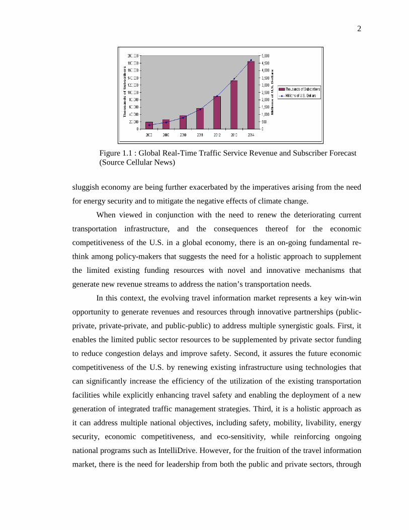
Figure 1.1 : Global Real-Time Traffic Service Revenue and Subscriber Forecast (Source
Cellular News) .................................................................................................................... 2
Figure 2.1: Illustration to boundary condition: (a) deterministic boundary condition; (b)
stochastic boundary condition. .......................................................................................... 14
Figure 2.2 : Conceptual framework of the proposed methodology .................................. 16
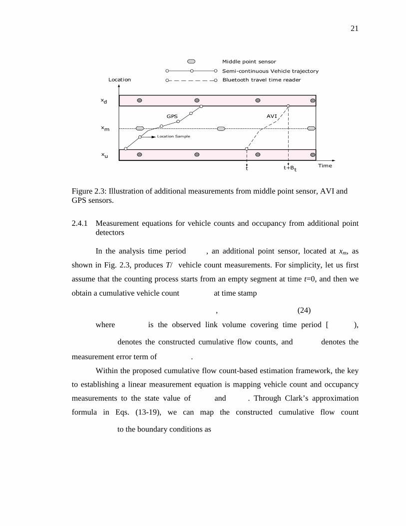
Figure 2.3: Illustration of additional measurements from middle point sensor, AVI and
GPS sensors. ..................................................................................................................... 21
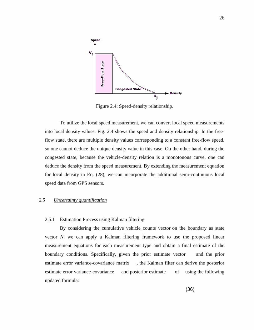
Figure 2.4: Speed-density relationship. ............................................................................ 26
Figure 2.5: A homogeneous segment used for conducting experiments (mile). .............. 29
Figure 2.6: Triangular shaped flow-density curve and the shockwave speeds in this
experiment ......................................................................................................................... 29
Figure 2.8: The original cell based density estimation profile. Color denotes the density
of each cell in veh/mile ..................................................................................................... 31
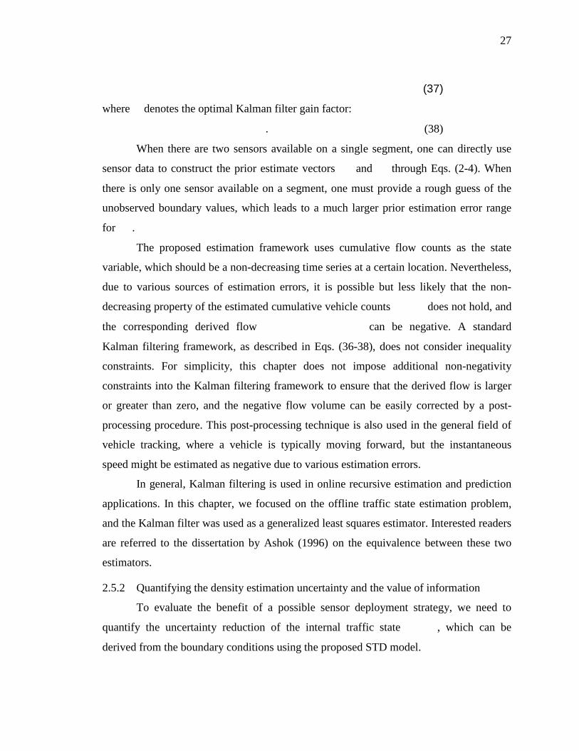
Figure 2.9: The original density uncertainty profile of cell based density estimation. Color
denotes the estimated density variance of each cell. ......................................................... 33
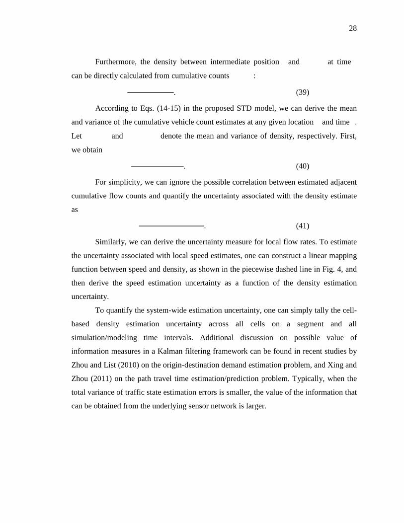
Figure 2.10: Value of Information vs. sampling time interval. (a) existing sensors; (b)
additional middle sensor. .................................................................................................. 34
Figure 2.11: Comparable total uncertainty reduction curve for GPS and AVI in different
market penetration rate. .................................................................................................... 35
Figure 2.12: A posterior estimation density uncertainty profile. Color denotes the
estimated density variance of each cell. ............................................................................ 35
Figure 3.1: Section-level travel time estimation ............................................................... 49
Figure 3.2: Conceptual framework and data flow ............................................................ 55
Figure 3.3: Steady-state travel time estimation variance .................................................. 62
Figure 3.4: Example of locating AVI sensors on a linear corridor ................................... 64
Figure 3.5: Numerical experiment results for regular traffic pattern estimation. ............. 68

vi
Figure 3.6: Comparison of different sensor location schemes (for regular traffic
estimation) ......................................................................................................................... 69
Figure 3.7: Numerical experiment results under recurring and non-recurring traffic
conditions .......................................................................................................................... 71

vii
LIST OF TABLES
Tables Page
Table 2.1: The comparative advantages of surveillance techniques ................................. 10
Table 2.2: Values of Clark’s approximation under different traffic mode / transition ..... 32
Table 3.1: Critical Path Travel Time Estimation Error under Existing and Optimized
Sensor Location Strategies ................................................................................................ 66
Table 4.1: List of variables and attributes that may impact traveler’s benefits from real-
time traffic information ..................................................................................................... 77
1
CHAPTER 1. INTRODUCTION
1.1
Under the aegis of Intelligent Transportation Systems (ITS), real-time traffic information
provision strategies are being proposed to manage traffic congestion, alleviate the effects
of incidents, enhance response efficiency after disasters, and improve the
multimodal/intermodal travel experience of travelers. Further, through innovations
enabled by leveraging technological advances in information and communications
technologies, such information provides travelers navigational capabilities and access to
location-based services. It enables travelers to enhance the quality and safety of their
travel experience through informed decision-making.
Background and motivation
Most existing traffic information provision and control systems are deployed and
maintained by public agencies, and are built on centralized management architectures.
The current technological advances and increased demand for real-time travel
information also provides the private sector an emerging domain of opportunities to
gainfully participate and shape the evolution of the nascent travel information market.
This market is expected to grow from 57 million real-time information users in 2010 to
more than 370 million globally by 2015 (Source: ABI Research). Further, the global
revenue from real-time traffic information services is projected to increase from $500
million in 2008 to $4.5 billion in 2014 (Source: Cellular News).
The evolution of the travel information market in the United States is occurring at a time
when limited revenue streams for federal funding of the transportation sector due to a
2
sluggish economy are being further exacerbated by the imperatives arising from the need
for energy security and to mitigate the negative effects of climate change.
When viewed in conjunction with the need to renew the deteriorating current
transportation infrastructure, and the consequences thereof for the economic
competitiveness of the U.S. in a global economy, there is an on-going fundamental re-
think among policy-makers that suggests the need for a holistic approach to supplement
the limited existing funding resources with novel and innovative mechanisms that
generate new revenue streams to address the nation’s transportation needs.
In this context, the evolving travel information market represents a key win-win
opportunity to generate revenues and resources through innovative partnerships (public-
private, private-private, and public-public) to address multiple synergistic goals. First, it
enables the limited public sector resources to be supplemented by private sector funding
to reduce congestion delays and improve safety. Second, it assures the future economic
competitiveness of the U.S. by renewing existing infrastructure using technologies that
can significantly increase the efficiency of the utilization of the existing transportation
facilities while explicitly enhancing travel safety and enabling the deployment of a new
generation of integrated traffic management strategies. Third, it is a holistic approach as
it can address multiple national objectives, including safety, mobility, livability, energy
security, economic competitiveness, and eco-sensitivity, while reinforcing ongoing
national programs such as IntelliDrive. However, for the fruition of the travel information
market, there is the need for leadership from both the public and private sectors, through
Figure 1.1 : Global Real-Time Traffic Service Revenue and Subscriber Forecast (Source Cellular News)

3
integrated policy decisions, development of standards, and the alignment of institutional
processes.
1.2
Currently, most of the real-time traffic information provision and control systems
infrastructure is deployed and maintained by public agencies. Given the projected growth
and profitability due to the evolution of the information services market in the near
future, the potential for new innovations and significant investments from the private
sector in emerging technologies and applications related to real-time traffic information
can foster new businesses. For this to happen at a widespread scale, there is need for
policy and regulatory decisions at the federal level. This study aims to exploit the synergy
due to innovative data collection, traffic management, and road pricing/credit
mechanisms that can encourage mutually beneficial information-sharing under innovative
partnerships (public-private sector, private-private sector, public–public sector
partnerships).
Chapter objectives
Two major issues will be investigated under different levels of public-private data
sharing plan and probe data availability: (1) how to use spatially distributed mobile probe
data to identify information gap and deficiency in terms of data quality, coverage and
reliability for an existing DOT traffic sensor network; (2) develop information-theoretical
sensor network design and management algorithms to determine where and which type of
DOT sensor investments should be made. The goal of sensor location optimization is to
maximize the expected information gain for the traffic state estimation and problem
applications; the sensor design model in this research will explicitly take into account the
uncertainty.
Further, the final goal of the proposed research work is to measure and understand
the benefits of real-time traffic information to the commuter by investigating the physical
and psychological benefits of real-time information by developing reliable traveler
behavior models that can be used to predict costs and benefits for real-world deployment.

4
1.3
The remainder of the research is organized as follows. Chapter 2 is on multi-
source traffic state estimation framework and fusion of data from multiple data sources.
Chapter 3 investigates sensor location optimization is to maximize the expected
information gain for the traffic state estimation. In Chapter 4, we seek to understand the
potential benefits of real-time information to travelers beyond mere physical benefits.
This chapter is about work-in-progress as this is the first year report of multiple year
effort and Chapter 5 draws conclusions from the study as well as discusses future work.
Organization of the research
5
CHAPTER 2. MULTI-SOURCE TRAFFIC STATE ESTIMATION FRAMEWORK
Existing in-pavement and road-side traffic sensors are typically located on a small
subset of freeway links and experience perceivable failure rates in the context of traffic
management/operations. Hence, while accurate travel time and traffic flow information
on ramps and arterial corridors are critically needed, they are expensive to collect on a
network-wide basis in addition to the reliability issues. The new generation of GPS-
enabled mobile devices presents a data-rich environment for regional traveler information
systems to accurately measure route-based travel times and network-wide traffic flow
dynamics and evolution. This research focuses on how to use multiple data sources,
including loop detector counts, AVI Bluetooth travel time readings and GPS location
samples, to estimate microscopic traffic states on a homogeneous freeway segment. A
multinomial probit model and an innovative use of Clark’s approximation method were
introduced to extend Newell’s method to solve a stochastic three-detector problem. The
mean and variance-covariance estimates of cumulative vehicle counts on both ends of a
traffic segment were used as probabilistic inputs for the estimation of cell-based flow and
density inside the space-time boundary and the construction of a series of linear
measurement equations within a Kalman filtering estimation framework. We present an
information-theoretic approach to quantify the value of heterogeneous traffic
measurements for specific fixed sensor location plans and market penetration rates of
Bluetooth or GPS flow car data.
This chapter is organized as follows. After reviewing the highway traffic state
estimation problem in Section 2.1, Section 2.2 briefly reviews the deterministic three-
detector model, which is based on the triangular relationship and Newell’s method. In
Sections 2.3, 2.4 and 2.5, we sequentially discuss stochastic boundary conditions and
6
propose a generalized least squares estimation framework to solve the stochastic three-
detector problem using heterogeneous data sources. In Section 2.6, numerical
experiments are used to demonstrate the proposed methodology and illustrate
observability improvements under different sensing plans and market penetration rates.
2.1
By reducing traffic system instability and volatility, the transportation system will
operate more efficiently, with better end-to-end trip travel time reliability and reduced
total emissions. By closely monitoring and reliably estimating the state of the system
using heterogeneous data sources, it is possible to apply information provision and
control actions in real time to best utilize the available highway capacity. These two
realizations have motivated the two main directions of this research: estimating freeway
traffic states from heterogeneous measurements and quantifying the uncertainty of traffic
state estimations under different sensor network deployment plans.
Literature Review
A majority of modeling methods focus on macroscopic point bottleneck detection
and link-level travel time estimation problems (e.g., Ashok and Ben-Akiva, 2000; Zhou
and List, 2010; Coifman, 2002). Recently, a number of data-mining methods have been
proposed for the purpose of obtaining microscopic traffic states on freeway segments
using different sources of data.
A generic microscopic traffic state estimation method consists of a number of key
components: an underlying traffic flow model, a state variable representation, and a
system process and a measurement equation. Different traffic flow models could lead to
various system state representation and process equations. For example, the Cell
Transmission Model (CTM), proposed by Daganzo (1994), captures the transfer flow
volume between cells as a minimum of sending and receiving flows, while Newell’s
simplified kinematic wave model (Newell, 1993), or three-detector method, which has
been systematically described by Daganzo (1997), considers cumulative vehicle counts at
an intermediate location of a homogeneous freeway segment as a minimization function
of the upstream and downstream cumulative arrival and departure counts.

7
To apply computationally efficient filters (e.g., a Kalman filter or particle filter) to
handle large-volume streaming sensor data, one of the major modeling challenges for
traffic state estimation is how to extract or construct linear system processes and
measurement equations. The widely used Eulerian sensing framework (e.g., Muñoz et al.,
2003; Sun et al., 2003; Sumalee et al., 2011) uses linear measurement equations to
incorporate flow and speed data from point detectors, while the emerging Lagrangian
sensing framework (e.g., Nanthawichit et al., 2003; Work et al., 2010; Herrera and
Bayen, 2010) aims to establish linear measurement equations to utilize semi-continuous
samples from moving observers or probes.
Muñoz et al. (2003) proposed a novel switching-mode model (SMM), which
adapts a Modified Cell Transmission Model (MCTM) to describe traffic dynamics and
transforms its nonlinear (minimization) state equations into a set of piecewise linear
equations. In particular, each set of linear equations is referred to as a mode, and the
SMM switches between different modes according to the detailed congestion status of the
cells in a section and the values of the mainline boundary inputs. Along this line, Sun et
al. (2003) employed a mixture Kalman filter to approximate the probabilistic state space
through a finite number of mode sample sequences, where the weight of each sample is
dynamically adjusted to reflect the posterior probability of all state vectors. Sumalee et al.
(2011) further introduced stochastic elements to the MCTM framework by Muñoz et al.
(2003) and proposed a stochastic cell transmission model.
Based on a second-order traffic flow model, Wang and Papageorgiou (2005) and
Wang et al. ( 2007) presented a comprehensive extended Kalman filter framework for the
estimation and prediction of highway traffic states. To construct linear process equations,
linearization around the current state (typically segment density) is required to determine
the outgoing flows between segments. Mihaylova et al. (2007) developed a CTM-based
second-order macroscopic model and adopted an alternative particle-filtering framework
to avoid computational intensive linearization operations.
Nanthawichit et al. (2003) conducted an early chapter that used Payne’s traffic
flow model and Kalman filtering within a Lagrangian sensing framework. Work et al.
(2010) derived a velocity-based partial differential equation (PDE) to construct linear
8
measurement equations for utilizing Lagrangian data, while an Ensemble Kalman filter
was embedded to propagate non-linear state equations through a Monte Carlo simulation
approach. Herrera and Bayen (2010) incorporated a correction term to the Lighthill-
Whitham-Richards partial differential equation (Lighthill and Whitham, 1955; Richards,
1956) to reduce the discrepancy between the Lagrangian measurements and the estimated
states. Treiber and Helbing (2002) proposed an efficient interpolation method by first
employing a “kernel function” to build the state equation for forward and backward
waves, and then integrating these two equations into a linear state equation through a
speed measurement-based weighting scheme. Based on the cumulative flow count and
simplified kinematic wave model (Newell, 2003), Coifman (2002) developed methods to
reconstruct vehicle trajectories from the measured local speed measures or a partial set of
vehicle probe trajectories. While Mehran et al. (2011) further investigated the sensitivity
impact of input data uncertainty, their solution framework has not directly taken into
account the measurement errors of different data sources.
While significant progress has been made in formulating system process and
measurement equations for the freeway traffic state estimation problem, this chapter aims
to address several challenging theoretical and practical issues.
First, we propose a stochastic version of Newell’s three-detector model to utilize
multiple data sources to estimate microscopic traffic states for a homogeneous freeway
segment. This method provides a new alternative to the existing CTM-based traffic state
estimation approach and the interpolation method of Treiber and Helbing (2002). In
particular, the traffic state of any intermediate point on a freeway segment can be
estimated directly from the boundary conditions through a minimization operation. To
handle the upstream and downstream cumulative flow counts as two random variables,
we introduce a multinomial probit model and Clark’s approximation (from the field of
discrete choice modeling) to approximate the minimization of two random variables as a
third random variable with quantifiable mean and variance. By doing so, we could link
the accuracy of traffic state estimation for each cell directly with the variability of the
boundary conditions.
9
Second, this chapter aims to incorporate emerging Automatic Vehicle
Identification (AVI) and Global Positioning System (GPS) data to estimate the inside
microscopic states of a traffic segment. There are a number of surveillance techniques
available for the purposes of traffic monitoring and management. Each technique has the
ability to collect and process specific types of real-time traffic data. AVI data, which are
obtainable from mobile phone Bluetooth samples, represent an emerging data source, but
they have been mainly used in link-based travel time estimation applications (e.g.,
Wasson et al., 2008, Haghani et al., 2010) or origin-destination demand estimation (e.g.,
Zhou and Mahmassani, 2006) rather than in the estimation of within-link traffic states,
such as cell-based density. The existing Lagrangian sensing framework (Nanthawichit et
al., 2003; Work et al., 2010; Herrera and Bayen, 2010) can map location-based speed
samples to a moving observer-oriented PDE system, but it has difficulties in
incorporating end-to-end time-dependent travel time records from AVI readers across a
series of cells.
It is practically important but theoretically challenging to utilize AVI data. In our
proposed approach, both AVI and GPS samples can be viewed as “bridges” between the
upstream and downstream boundaries in terms of cumulative flow counts. Specifically,
we develop a series of linear measurement equations within the proposed stochastic
three-detector approach that can dramatically simplify the process of estimating the
likelihood of free-flow vs. congested traffic conditions for any location inside a traffic
segment. Third, the value of information (VOI) for the highway traffic state estimation
problem systematically investigated for various types of data sources. We use an
information-theoretic approach to quantify the uncertainty of microscopic traffic state
estimation results and further evaluate the effectiveness of various important sensor
design scenarios, such as point detector sampling rates, AVI market penetration rates, and
GPS market penetration rates.
Table 2.1 summarizes the data measurement types and comparative advantages of
estimating traffic states at different resolutions. Each of these data sources has strengths
and weaknesses, and an effective traffic state monitoring system must be able to fuse
multiple data streams to symmetrically capture traffic system instability and volatility.

10
Moreover, as more sensing technologies become available, the monitoring system must
be able to seamlessly incorporate them into a computationally efficient and theoretically
rigorous analysis framework.
Table 2.1: The comparative advantages of surveillance techniques
Surveillance Type
Measurement Type Data Quality Costs and Concerns
Point Detectors Vehicle counts and point speed
High accuracy and relatively low
reliability
High maintenance cost
Automatic Vehicle
Identification
Point to point flow information for tagged vehicles such as travel
time and volume
Accuracy depends on market
penetration level of tagged vehicles
Relatively high installation costs for automated vehicle ID
reader Mobile GPS
location sensors Semi-continuous path trajectory for
individual equipped vehicles
Accuracy depends on market
penetration level of probe vehicles
Public privacy concerns
Trajectory data from video
image processing
Continuous path trajectory for vehicles on
different lanes
Accuracy depends on machine vision
algorithms
Relatively high installation cost for
overhead video camera and communication
wires
2.2
2.2.1 Parameters of traffic flow model
Problem statement and conceptual framework
= Free-flow speed in the free-flow state. = Backward wave speed in the congestion state.
= Jam density or maximum density, where the flow reduces to zero. FFTT= Time for traversing a certain distance by a forward wave with speed . BWTT= Time for traversing a certain distance by a backward wave with speed . 2.2.2 Subscripts and parameters of space-time representation
= Unit space increment, i.e., length of one section. = Space index of sections, . = Space position of section , i.e., . = Location of upstream boundary, . = Location of downstream boundary, .

11
= Distance from a point x to the downstream boundary , . = Unit time increment, i.e., length of one simulation clock time.
= Point sensor sampling time interval, i.e., 1 s, 30 s, 5 min. = Time index of simulation, . = Time index of sampling point, . = Time, starting from zero, , . = Measurement deviation of AVI (e.g., Bluetooth) travel time readers. = GPS sampling time interval for a semi-continuous vehicle trajectory.
2.2.3 Boundary measurements and variables
, = Measured vehicle counts between time and at location and , respectively.
, = True vehicle counts between time and at location and , respectively.
), )= Measurement error of vehicle counts and , assumed to be normally distributed.
, = Measured cumulative vehicle counts at location and location , respectively, at timestamp .
, = True cumulative vehicle counts at location and , respectively, at timestamp .
, = Error term of and , to be derived as normally distributed random variables. 2.2.4 Estimation variables
= Cumulative vehicle counts at any intermediate position x at time t. , = Estimated mean and variance value of cumulative vehicle counts
. = Flow at position x at time t, to be derived from . , = Estimated mean and variance value of flow .
= Density at position x at time t, to be derived from . , = Estimated mean and variance value of density .
2.2.5 Variables used in probit model and Clark’s approximation
, = Disutility of the first and the second component of a minimization equation with two random variables.
, = Systematic disutility of disutility and . , = Noise of disutility and .
= Variance of the difference between systematic disutility and . = A combined variable, derived from using to divide the difference between
systematic disutility and . = Standard normal distribution of the combined variable .

12
= Cumulative normal curve of the combined variable . = A variable to denote the equation . = A variable to denote the equation
. 2.2.6 Vector and matrix forms in measurement models of the Kalman filtering
framework
= Cumulative vehicle counts vector on the upstream and downstream boundaries as the system state vector.
= Prior estimate vector of the mean values of . = Posterior estimate of the mean values of . = Prior estimate error covariance matrix of . = Posterior estimate error covariance matrix of .
= Complete sets of additional measurements, i.e., additional point sensor, AVI and GPS measurements.
= Sensor mapping matrix that connects system state vector N to measurement vector . = Optimal gain matrix of the Kalman filter. = Variance-covariance matrix of measurement errors of .
Consider a homogeneous freeway segment without enter or exit ramps in between.
The segment is divided into a number of sections of , , and is the
length of a section. The modeling time horizon is discretized into , ,
where denotes the modeling time index, and denotes the length of each simulation
time step. We use , to denote sampling time stamps, where denotes
the sampling time index, and represents the length of each sampling time interval, e.g.,
30 s or 5 min.
Two point sensor stations are located at upstream location and
downstream location . The measurement equation for the vehicle counts at the
upstream sensor can be expressed as
), where , (1)
where denotes the true vehicle counts at upstream sensor, and
denotes the measurement error term. is assumed to be normally distributed with
zero mean and a variance of .
Generally, the cumulative upstream vehicle counts at each sampling time stamp
can be derived from the observed vehicle counts:

13
, (2)
where the summation of multiple normal random independent
variables is the error of measured cumulative vehicle counts at sampled time .
Because the sum of multiple normally distributed independent variables is normally
distributed, the cumulative vehicle count follows a normal distribution.
To construct the cumulative vehicle counts at the non-sampled time stamps, we
employed a linear interpolation method, shown below. For a time stamp
, the corresponding cumulative vehicle counts can be derived as follows:
. (3)
Assuming the upstream detector produces unbiased measurements, we can
express the mean value of a continuous cumulative arrival flow count as
. (4)
We can also derive the related error term , which is the combined error
source, including the measurement error
and the linear interpolation error.
Likewise, the cumulative departure flow count curve at the downstream station
can be constructed.
Given deterministic cumulative departure and arrival flow counts, and
, at the upstream and downstream detectors, the three-detector problem considered
by Newell (1993) aims to determine the traffic state at any intermediate detector location
. The traffic state at the third detector location x is represented by
cumulative flow count value , and cell-based density, flow and speed measures can
be derived easily as functions of .
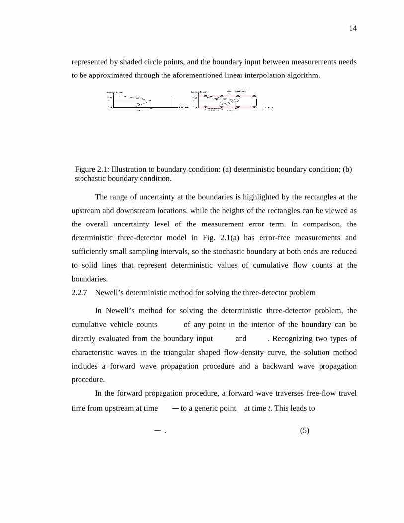
As demonstrated in Fig. 2.1(b), the stochastic three-detector (STD) problem needs
to estimate internal traffic states from its stochastic boundary inputs and ,
which include not only the measurement errors at the time stamps with data but also the
possible interpolation errors. For illustration purposes, the measurements with errors are
14
represented by shaded circle points, and the boundary input between measurements needs
to be approximated through the aforementioned linear interpolation algorithm.
The range of uncertainty at the boundaries is highlighted by the rectangles at the
upstream and downstream locations, while the heights of the rectangles can be viewed as
the overall uncertainty level of the measurement error term. In comparison, the
deterministic three-detector model in Fig. 2.1(a) has error-free measurements and
sufficiently small sampling intervals, so the stochastic boundary at both ends are reduced
to solid lines that represent deterministic values of cumulative flow counts at the
boundaries.
2.2.7 Newell’s deterministic method for solving the three-detector problem
In Newell’s method for solving the deterministic three-detector problem, the
cumulative vehicle counts of any point in the interior of the boundary can be
directly evaluated from the boundary input and . Recognizing two types of
characteristic waves in the triangular shaped flow-density curve, the solution method
includes a forward wave propagation procedure and a backward wave propagation
procedure.
In the forward propagation procedure, a forward wave traverses free-flow travel
time from upstream at time to a generic point at time t. This leads to
. (5)
Figure 2.1: Illustration to boundary condition: (a) deterministic boundary condition; (b) stochastic boundary condition.
15
In the backward wave propagation procedure, a backward wave is emitted from
the downstream boundary to the generic point x at time t inside the boundary. Because
the wave pace of the backward wave is equal to , and the density along the backward
wave is (according to the triangular shaped flow-density relationship), we have
. (6)
Considering as the distance from the downstream boundary to a point x inside
the boundary, Newell’s method selects the smallest value of between estimated
values from the forward and backward wave propagation procedure:
. (7)
If either procedure leads to a flow that exceeded the capacity at ,
one needs to restrict by a straight line with a slope equal to the capacity at .
Hurdle and Son (2001, 2002) and Son (1996) demonstrated the effectiveness and
tested the computational efficiency of Newell’s method using field data. Daganzo (2003,
2005) presented an extension to the variational formulation of kinematic waves, where
the fundamental diagram is relaxed to a concave flow-density relationship. Furthermore,
Daganzo (2006) showed the equivalence between the kinematic wave with a triangular
fundamental diagram and a simplified linear car, following a model similar to the one
proposed by Newell (2002).
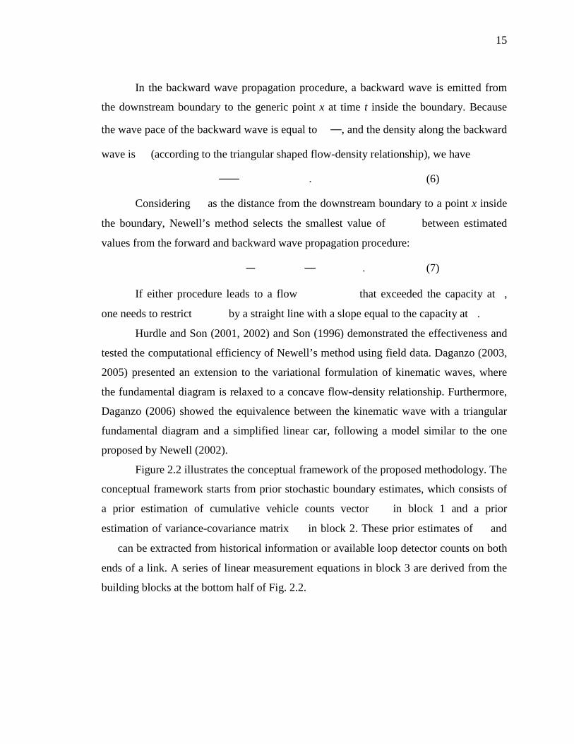
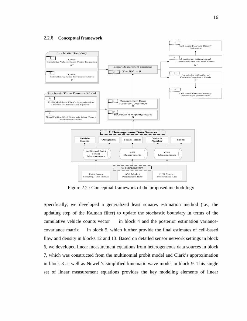
Figure 2.2 illustrates the conceptual framework of the proposed methodology. The
conceptual framework starts from prior stochastic boundary estimates, which consists of
a prior estimation of cumulative vehicle counts vector in block 1 and a prior
estimation of variance-covariance matrix in block 2. These prior estimates of and
can be extracted from historical information or available loop detector counts on both
ends of a link. A series of linear measurement equations in block 3 are derived from the
building blocks at the bottom half of Fig. 2.2.
16
2.2.8 Conceptual framework
Stochastic Boundary
A priori Estimation Variance-Covariance Matrix
A priori Cumulative Vehicle Count Vector Estimation
N −
P−
1
2A posterior estimation of
Variance-Covariance Matrix
A posterior estimation ofCumulative Vehicle Count Vector
N +
P+
4
5
Linear Measurement Equations
Y HN R−= +3
Cell Based Flow and DensityEstimation
Cell Based Flow and DensityUncertainty Quantification
12
13
AVI Measurements
Travel Times
Additional Point Sensor
Measurements
Vehicle Counts Occupancy
GPS Measurements
Vehicle Number Speed
7. Heterogeneous Data Sources
Stochastic Three Detector Model
Newell’s Simplified Kinematic Wave TheoryMinimization Equation
Probit Model and Clark’s ApproximationSolution to a Minimization Equation
8
9 Boundary N Mapping Matrix H
Measurement Error Variance Covariance
R
Point Sensor Sampling Time Interval
AVI Market Penetration Rate
GPS Market Penetration Rate
10
11
6. Parameters
Specifically, we developed a generalized least squares estimation method (i.e., the
updating step of the Kalman filter) to update the stochastic boundary in terms of the
cumulative vehicle counts vector in block 4 and the posterior estimation variance-
covariance matrix in block 5, which further provide the final estimates of cell-based
flow and density in blocks 12 and 13. Based on detailed sensor network settings in block
6, we developed linear measurement equations from heterogeneous data sources in block
7, which was constructed from the multinomial probit model and Clark’s approximation
in block 8 as well as Newell’s simplified kinematic wave model in block 9. This single
set of linear measurement equations provides the key modeling elements of linear
Figure 2.2 : Conceptual framework of the proposed methodology

17
measurement matrix in block 10 and measurement error variance and covariance
matrix in block 11.
2.3
Solving stochastic three-detector model using the multinomial probit model and
Clark’s approximation
By extending Newell’s deterministic three-detector model as shown in Fig. 1(a),
this section presents the model and solution algorithms for an STD problem, which aims
to estimate the traffic state at any intermediate location on a homogeneous
freeway segment using available measurements with various degrees of measurement
errors. Mathematically, the proposed STD problem needs to consider a stochastic version
of Eq. (7):
, (8)
where both cumulative arrival and departure flow counts are Normal random
variables, as shown previously,
, and (9)
. (10)
The key to solving the proposed Eq. (8) is the development of efficient
approximation methods to estimate the cumulative vehicle counts at location at
time . By assuming that the maximum of two normally distributed random variables can
be approximated by a third normally distributed random variable, Clark (1961) proposed
an approximation method to calculate the mean and variance (i.e., the first two moments)
of the third Normal variable. In the field of discrete choice modeling (Daganzo, 1979), a
multinomial probit model has been widely used to calculate the choice probability of an
alternative based on a utility-maximization or a disutility-minimization framework, where
the unobserved terms of alternative utilities are assumed to be normal distributions with
possible correlation and heteroscedasticity structures. Daganzo et al. (1977) and Horowitz

18
et al. (1982) investigated the numerical accuracy of Clark’s approximation under a small
number of alternatives.
By reformulating Eq. (8) within a disutility-minimization framework, the
cumulative vehicle count is the minimum of the above two disutilities,
corresponding to the forward wave and backward wave alternatives.
, (11)
where
and . (12)
It is easy to verify that the systematic disutility and
, respectively, correspond to the forward or backward wave
propagation procedures in Eqs. (5-6). The unobserved terms can be derived as
and .
In this probit model framework, the choice probability of each alternative is
equivalent to the probability of the forward wave vs. the backward wave being selected to
determine the traffic state (i.e., free-flow vs. congested) of the current time-space location
(t, x). In this chapter, we further adopted Clark’s approximation method to estimate the
mean and variance of the estimated cumulative flow count as
, (13)
where the mean
(14)
and the variance
. (15)
Based on the notation system used in Sheffi (1985), the coefficients and
can be further calculated by the following formulas.
; (16)
(17)
There are several elements in Eqs. (16-17), including

19
(i) a parameter describing the standard deviation of the systematic disutility
difference :
, (18)
where and denote the variance of and , respectively, and is the
correlation coefficient between the error terms and ;
(ii) a standardized normal variable
, (19)
(iii) a corresponding standard normal distribution function
and a cumulative normal distribution curve
. (20)
In particular, Eq. (16) also show that the relative weights for the systematic
disutilities and in the final mean estimate are jointly determined by the
cumulative distribution functions and as well as an adjustment factor of
that ranges between 0 and 1.
Because the deterministic three-detector model is a special case of the proposed
STD model with error-free measurement, we can substitute =0 and into Eqs.
(14-20) to obtain the mean and variance of cumulative flow count in the following
relationships between and :
.
(21)
. (22)
When solving the deterministic three-detector model by Clark’s approximation
method, we obtain an error-free cumulative vehicle count through the simple
minimization operation. This derivation confirms that the proposed method using Clark’s
approximation can satisfactorily handle the deterministic three-detector model as a
special case of the STD model.
20
2.4
Measurement models for heterogeneous data sources
Corresponding to blocks 8 and 9 of the conceptual framework in Fig. 2.2, the
previous session proposed approximation formulas that can connect internal state
with the stochastic boundary conditions. This session proceeds to establish a set of linear
measurement equations that can map additional sensor measurements to the boundary
conditions and . The following discussions detail the modeling components
for blocks 3, 10 and 11 in Fig. 2 regarding the linear measurement equations shown
below.
, where . (23)
Specifically, measurement vector can include flow counts and occupancy from
additional point detectors, Bluetooth reader travel time measurements, and GPS vehicle
trajectory data. Matrix provides a linear map between cumulative vehicle counts on the
boundary, namely and and observations Y. The measurement error
covariance matrix R is referred to as the combined error that includes error sources such
as sensor measurement errors and approximation errors in the proposed modeling
approach.
In general, more measurements would lead to less uncertainty in the boundary
conditions. Fig. 2.3 illustrates three typical sensing configurations to reduce the
estimation errors in the freeway traffic state estimation problem:
(i) deploying an additional point detector at the intermediate location, which can
produce vehicle counts and occupancy measurements;
(ii) installing two prevailing AVI (e.g., mobile phone Bluetooth) readers, which
can detect passing time stamps of individual vehicles;
(iii) equipping a certain percentage of vehicles with GPS mobile devices, which
can produce semi-continuous vehicle trajectories for a short sampling interval,
e.g., every 10 seconds.
21
2.4.1 Measurement equations for vehicle counts and occupancy from additional point detectors
In the analysis time period , an additional point sensor, located at xm, as
shown in Fig. 2.3, produces T/ vehicle count measurements. For simplicity, let us first
assume that the counting process starts from an empty segment at time t=0, and then we
obtain a cumulative vehicle count at time stamp
, (24)
where is the observed link volume covering time period [ ),
denotes the constructed cumulative flow counts, and denotes the
measurement error term of .
Within the proposed cumulative flow count-based estimation framework, the key
to establishing a linear measurement equation is mapping vehicle count and occupancy
measurements to the state value of and . Through Clark’s approximation
formula in Eqs. (13-19), we can map the constructed cumulative flow count
to the boundary conditions as
Figure 2.3: Illustration of additional measurements from middle point sensor, AVI and GPS sensors.

22
, (25)
where the combined error term includes both the measurement error
and the estimation error in Clark’s approximation, . Within the linear
measurement framework
, where , (26)
we can construct a transformed measurement of
, the mapping vector , and the system state vector
As an extension, if there are vehicles on the segment at time t=0, then we can
reset =0 and adjust cumulative flow counts from the middle sensor to consider
the additional number of vehicles that have already passed through but have not
reached the end of segment
A dual loop detector that includes two detectors at location and ,
where l is the distance of the two detectors yields occupancy measurements that can be
converted into local density (Cassidy and Coifman, 1997). By expressing
the local density at time at location as a function of the estimated cumulative
vehicle count and
, (27)
we obtain the following linear measurement equations.
- - - - (28)
where the error term is the combination error term, including the measurement error
and estimation error of and .

23
Unlike the standard linear mapping equation with a constant mapping matrix H,
the mapping coefficients and in Eqs. (23) and (26) are dependent on the
prevailing traffic conditions on the boundary, namely, the difference between
and . Because the true values of cumulative flow counts are unknown,
only the estimates of cumulative departure and arrival flow counts are available to
calculate and when constructing the linear measurement equations. This
possible estimation error, associated with the boundary cumulative flow counts,
introduces one more source of error that should be included in the combined error terms
and . On the other hand, as demonstrated in Eq. (21), when the standardized difference
between and , as shown in Eq. (19), is significantly large, the
coefficients and take extreme values of 0 or 1, indicating that the internal
condition at position (t,x) can be estimated directly from one of the forward vs. backward
wave propagation procedures with high confidence levels.
2.4.2 Measurement equation for AVI data
In this subsection, we show that the proposed methodology can effectively
incorporate the AVI (Bluetooth data) data source.
As illustrated in Fig. 2.3, two Bluetooth readers are separately located at the
upstream and downstream locations. For a tagged vehicle, its passing time stamps at the
two readers are denoted t and , respectively. To connect these samples with the
cumulative vehicle counts at the both ends (i.e., unknown state variable in the freeway
traffic state estimation problem), under a First-In-First-Out (FIFO) assumption for the
three-detector model, we can establish the following conditions to ensure that the tagged
vehicle has the same cumulative flow count number when passing through both the
upstream and downstream stations. Under an error-free environment, we have
, (29)
while consideration of a combined error term leads to
where (30)
24
and where is the covariance of error term .
The combined error term includes possible deviation in identifying and
. To calculate the error range in identifying , we first denote as a
constant value for the likely feasible range of AVI readers’ clock drift errors and
as the average flow rate around time . Then, the standard deviation of the flow count
deviation during a time duration of possible clock drifts is . According to Eq.
(15), we can further consider the estimation uncertainty of and (before
incorporating AVI data) as and . Thus, the variance of the
combined error can be approximated as
. (31)
In this case, a linear measurement equation can be established as follows:
, where . (32)
Note that the measurement term in the above form is expressed as rather
than the original passing time stamp samples. Additionally, the mapping vector
, and the system state vector . To consider AVI
reader stations that are not located on the boundaries of segments, we can first map the
passing time stamp measurements to the cumulative flow counts corresponding to the
AVI reader locations, say, and , where and are upstream and
downstream locations of AVI readers. The second step is to connect and
to the cumulative arrival and departure curves and at the
boundary using the proposed stochastic three-detector model.
2.4.3 Measurement equation for GPS probe data
GPS probe data offer a semi-continuous trajectory of a vehicle in a segment. This
section first extends the cumulative vehicle count-based approach in the previous section
to construct measurement equations for each sample point along the trajectory. Second,
we aim to use the local speed profile of the vehicle in our estimation framework.
As shown in Fig. 2.3, a vehicle of number traverses the segment along semi-
continuous trajectory , , where denotes the sampling time
25
interval of GPS, and denotes total number of sampling points for an individual vehicle
trajectory.
By applying the proposed STD model, we can map the cumulative vehicle count
m at a sampling point with the following boundary conditions:
, (33)
where the combined error term should include the following: (1) GPS location
measurement errors; (2) the estimation error associated with the entry vehicle count m;
and (3) the estimation error of cumulative vehicle counts through
the proposed STD model. The second type of error range can be approximated using a
similar formula for AVI data, i.e., . According to Eq. (15), the variance of the
third estimation error is
. (34)
Similar to the previous analysis, we can establish a linear measurement equation,
shown below.
, where (35)
and where the transformed measurement term is
, the system state vector
.
Typically, the location data of GPS probes are available second by second, and
the adjacent locations of two sample points are used to compute the local speed measure.
However, to reduce battery consumption and mitigate privacy concerns, some practical
systems use a much longer time interval for data reporting, i.e., 30 seconds or 1 minute,
while still sending local speed data (calculated from the internal second-by-second
location data) to the data server.
26
To utilize the local speed measurement, we can convert local speed measurements
into local density values. Fig. 2.4 shows the speed and density relationship. In the free-
flow state, there are multiple density values corresponding to a constant free-flow speed,
so one cannot deduce the unique density value in this case. On the other hand, during the
congested state, because the vehicle-density relation is a monotonous curve, one can
deduce the density from the speed measurement. By extending the measurement equation
for local density in Eq. (28), we can incorporate the additional semi-continuous local
speed data from GPS sensors.
2.5
Uncertainty quantification
2.5.1 Estimation Process using Kalman filtering
By considering the cumulative vehicle counts vector on the boundary as state
vector N, we can apply a Kalman filtering framework to use the proposed linear
measurement equations for each measurement type and obtain a final estimate of the
boundary conditions. Specifically, given the prior estimate vector and the prior
estimate error variance-covariance matrix , the Kalman filter can derive the posterior
estimate error variance-covariance and posterior estimate of using the following
updated formula:
(36)
Figure 2.4: Speed-density relationship.
27
(37)
where denotes the optimal Kalman filter gain factor:
. (38)
When there are two sensors available on a single segment, one can directly use
sensor data to construct the prior estimate vectors and through Eqs. (2-4). When
there is only one sensor available on a segment, one must provide a rough guess of the
unobserved boundary values, which leads to a much larger prior estimation error range
for .
The proposed estimation framework uses cumulative flow counts as the state
variable, which should be a non-decreasing time series at a certain location. Nevertheless,
due to various sources of estimation errors, it is possible but less likely that the non-
decreasing property of the estimated cumulative vehicle counts does not hold, and
the corresponding derived flow can be negative. A standard
Kalman filtering framework, as described in Eqs. (36-38), does not consider inequality
constraints. For simplicity, this chapter does not impose additional non-negativity
constraints into the Kalman filtering framework to ensure that the derived flow is larger
or greater than zero, and the negative flow volume can be easily corrected by a post-
processing procedure. This post-processing technique is also used in the general field of
vehicle tracking, where a vehicle is typically moving forward, but the instantaneous
speed might be estimated as negative due to various estimation errors.
In general, Kalman filtering is used in online recursive estimation and prediction
applications. In this chapter, we focused on the offline traffic state estimation problem,
and the Kalman filter was used as a generalized least squares estimator. Interested readers
are referred to the dissertation by Ashok (1996) on the equivalence between these two
estimators.
2.5.2 Quantifying the density estimation uncertainty and the value of information
To evaluate the benefit of a possible sensor deployment strategy, we need to
quantify the uncertainty reduction of the internal traffic state , which can be
derived from the boundary conditions using the proposed STD model.
28
Furthermore, the density between intermediate position and at time
can be directly calculated from cumulative counts :
. (39)
According to Eqs. (14-15) in the proposed STD model, we can derive the mean
and variance of the cumulative vehicle count estimates at any given location and time .
Let and denote the mean and variance of density, respectively. First,
we obtain
. (40)
For simplicity, we can ignore the possible correlation between estimated adjacent
cumulative flow counts and quantify the uncertainty associated with the density estimate
as
. (41)
Similarly, we can derive the uncertainty measure for local flow rates. To estimate
the uncertainty associated with local speed estimates, one can construct a linear mapping
function between speed and density, as shown in the piecewise dashed line in Fig. 4, and
then derive the speed estimation uncertainty as a function of the density estimation
uncertainty.
To quantify the system-wide estimation uncertainty, one can simply tally the cell-
based density estimation uncertainty across all cells on a segment and all
simulation/modeling time intervals. Additional discussion on possible value of
information measures in a Kalman filtering framework can be found in recent studies by
Zhou and List (2010) on the origin-destination demand estimation problem, and Xing and
Zhou (2011) on the path travel time estimation/prediction problem. Typically, when the
total variance of traffic state estimation errors is smaller, the value of the information that
can be obtained from the underlying sensor network is larger.

29
2.6
Numerical Experiments
In this section, we used a set of simulated experiments to investigate the
performance of the proposed STD model on a 0.5-mile homogeneous segment with no
entry or exit ramps, as shown in Fig. 2.5. The segment is divided into 10 sections, and the
time of interest ranges from 0 to 1,200 s. Two loop detectors are installed at the upstream
and downstream ends.
section 10section 2 section 3 section 4 section 5 section 6 section 7 section 8 section 9section 1
0x = 0.45x =0.05x = 0.1x = 0.15x = 0.2x = 0.25x = 0.3x = 0.35x = 0.4x = 0.5x =
upstream downstream
Figure 2.5: A homogeneous segment used for conducting experiments (mile).
The other important parameters include a triangle-shaped flow-density relation, as shown
in Fig. 2.6, where the free-flow speed , the backward wave speed
and the maximum density .
In this experiment, we consider a constant arriving flow rate
, while the downstream bottleneck discharge rate is assumed
to be time-dependent, i.e., .
0
500
1000
1500
2000
2500
0 20 40 60 80 100 120 140 160 180 200 220 240
Flow
(veh
icle
s/ho
ur)
Density (vehicles/mile/lane)
4 m/h
12 m/h
1200 veh/h t [0,1200]u = ∈ λ
600 veh/h t [0,450]( )
1800 veh/h t [451,1200]tλ
∈= ∈
Figure 2.6: Triangular shaped flow-density curve and the shockwave speeds in this experiment
12 m/h
600
180
120

30
2.6.1 Estimations results of the STD model
Using the deterministic three-detector approach, the first step was to generate the
ground truth boundary conditions in terms of deterministic arrival and departure
cumulative vehicle count curves, as shown in Fig. 2.7. In particular, there are three
shockwaves:
(1) The first shockwave travels at a speed of 4 m/h, resulting in a long queue
in the segment. When it finally spills back to the upstream site, the flow detected at the
upstream sensor (compared to the actual arrival flow of 1,200 veh/h) is controlled by the
bottleneck capacity of 600 veh/h.
(2) The second backward recovery shockwave starts to propagate upstream at
a speed of 12 m/h, right after the bottleneck capacity recovers to 1,800 veh/h at a time of
451 s.
(3) The third shockwave is triggered by the transition where the arrival rate of
1,200 veh/h, starting at a time of 701 s, is lower than the normal bottleneck capacity
The second step is to test the ability to capture the shockwave propagation using
the proposed STD model. The corresponding stochastic boundary conditions, in terms of
prior estimation cumulative vehicle counts vector and a prior estimation variance-
covariance matrix , were constructed under a sampling time interval min = 300
s, with a +/−10% measurement standard deviation . Based on and , the STD model
is able to produce the cell-based density estimates for all 10 sections inside the segment,
shown in Fig. 2.8, and the corresponding uncertainty range for each cell in the space-time
diagram, shown in Fig. 2.9.
As expected, Fig. 2.8 clearly shows the transition of the following four regimes:
(1) free-flow (FF); (2) severe congestion (SC); (3) mild congestion (MC); and (4) free-
flow. The boundaries of those regimes correspond to the underlying shockwaves.
To further demonstrate the computational details of the proposed STD model, let
us consider a series of time stamp points at section 8, marked in Fig. 2.8. These seven
points are numbered by time from 1 to 7, and each point corresponds to a particular
traffic mode. Specifically, four points of interest, 1, 3, 5 and 7, are under the steady traffic

31
state mode, and the other three points are in the transition boundaries. Table 2 shows the
values of Clark’s approximation for estimating the mean and variance of the cumulative
flow count using Eqs. (20-22).
Figure 2.7: Arrival and departure cumulative vehicle count curves.
0
50
100
150
200
250
300
350
400
450 0 50
10
0 15
0 20
0 25
0 30
0 35
0 40
0 45
0 50
0 55
0 60
0 65
0 70
0 75
0 80
0 85
0 90
0 95
0 10
00
1050
11
00
1150
12
00
Cum
ulat
ive
Veh
icle
Cou
nt
Time (1 s)
Shockwave
Arrival curve
Departure curve
1
2
3
Figure 2.8: The original cell based density estimation profile. Color denotes the density of each cell in veh/mile.
FF FF MC SC

32
Table 2.2: Values of Clark’s approximation under different traffic mode / transition
Point Traffic Mode/Transition
Time (min)
1 FF 2 0 1 0 33.33 45.83 2 FF SC 3.3 0.3 0.5 0.5 58.33 58.33 3 SC 6 0 0 1 113.3 85.83 4 SC MC 8.5 0 0 1 163.3 116.5 5 MC 11 0 0 1 205.1 191.5 6 MC FF 13.2 0.8 0.5 0.5 257.0 257.0 7 FF 16 0 1 0 313.3 328.6
In Eqs.15-17 for generating the final cumulative flow count estimates, the
cumulative normal distribution of the combined variable Φ(γ) and Φ(-γ) is the weights for
forward wave vs. backward wave alternatives. Based on the numerical results in Table
2.2, we have the following interesting findings.
(1) When the difference of systematic disutility, Vu and Vd, is significantly large, the
weight on each alternative, Φ(γ) and Φ(-γ), has an extreme value of zero or one, and the
corresponding adjustment factor αϕ(γ) is close to zero. It should be noted that, although
Table 2.2 shows a value of zero for αϕ(γ), it is actually a very small numerical value. By
substituting αϕ(γ)=0 into the mean and variance estimation equation in Eqs. 16-17, we
can verify that and for points 1 and 7, indicating that the
uncertainty of the final estimate is controlled by the dominating alternative.
(2) In cases of state transitions, i.e., free-flow to congested or congested to free-flow,
Φ(γ) and Φ(-γ) stay at a level of 0.5, leading to almost equal weights for each alternative,
and a positive adjustment factor αϕ(γ) is needed. More interestingly, this case results in a
large uncertainty or low confidence level about its exact value of the cumulative flow
count, and the variance is jointly determined by both alternatives.
The overall uncertainty plot in Fig. 2.9 for each cell confirms our findings; that is, the
boundaries of the state transition have large uncertainty. In addition, the estimation
generally increases when the time clock advances, as the measurement error in flow
counts from the previous time intervals must be included in the cumulative flow count
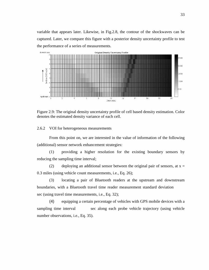
33
variable that appears later. Likewise, in Fig.2.8, the contour of the shockwaves can be
captured. Later, we compare this figure with a posterior density uncertainty profile to test
the performance of a series of measurements.
2.6.2 VOI for heterogeneous measurements
From this point on, we are interested in the value of information of the following
(additional) sensor network enhancement strategies:
(1) providing a higher resolution for the existing boundary sensors by
reducing the sampling time interval;
(2) deploying an additional sensor between the original pair of sensors, at x =
0.3 miles (using vehicle count measurements, i.e., Eq. 26);
(3) locating a pair of Bluetooth readers at the upstream and downstream
boundaries, with a Bluetooth travel time reader measurement standard deviation
sec (using travel time measurements, i.e., Eq. 32);
(4) equipping a certain percentage of vehicles with GPS mobile devices with a
sampling time interval sec along each probe vehicle trajectory (using vehicle
number observations, i.e., Eq. 35).
Figure 2.9: The original density uncertainty profile of cell based density estimation. Color denotes the estimated density variance of each cell.
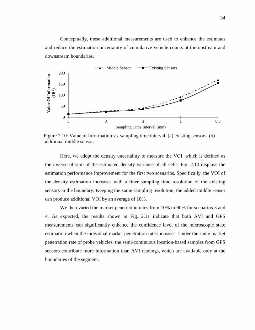
34
Conceptually, these additional measurements are used to enhance the estimates
and reduce the estimation uncertainty of cumulative vehicle counts at the upstream and
downstream boundaries.
Here, we adopt the density uncertainty to measure the VOI, which is defined as
the inverse of sum of the estimated density variance of all cells. Fig. 2.10 displays the
estimation performance improvement for the first two scenarios. Specifically, the VOI of
the density estimation increases with a finer sampling time resolution of the existing
sensors in the boundary. Keeping the same sampling resolution, the added middle sensor
can produce additional VOI by an average of 10%.
We then varied the market penetration rates from 10% to 90% for scenarios 3 and
4. As expected, the results shown in Fig. 2.11 indicate that both AVI and GPS
measurements can significantly enhance the confidence level of the microscopic state
estimation when the individual market penetration rate increases. Under the same market
penetration rate of probe vehicles, the semi-continuous location-based samples from GPS
sensors contribute more information than AVI readings, which are available only at the
boundaries of the segment.
0
50
100
150
200
5 3 2 1 0.5
Val
ue O
f Inf
orm
atio
n (1
0-9)
Sampling Time Interval (min)
Middle Sensor Existing Sensors
Figure 2.10: Value of Information vs. sampling time interval. (a) existing sensors; (b) additional middle sensor.

35
We now consider an integrated case with scenarios 2, 3 and 4 using the following
settings: existing loop detectors at boundaries with a 5-min sampling time interval, an
additional sensor at x = 0.3 miles with a 5-min sampling time interval, and a randomly
selected portion of vehicles (10%) that are equipped with AVI Bluetooth and GPS
sensors.
The proposed information-theoretic approach produces the posterior estimation
cumulative vehicle counts vector and variance-covariance matrix . Comparing the
0
20
40
60
80
100
120
140
0% 10% 20% 30% 40% 50% 60% 70% 80% 90%
Val
ue O
f Inf
orm
atio
n (1
0-9)
Market Penetration Rate (%)
GPS AVI
Figure 2.11: Comparable total uncertainty reduction curve for GPS and AVI in different market penetration rate.
Figure 2.12: A posterior estimation density uncertainty profile. Color denotes the estimated density variance of each cell.

36
original estimated density uncertainty profile in Fig. 2.9 and Fig. 2.12 for the above
integrated sensor network setting, we find that overall uncertainty has been dramatically
reduced, but the cells corresponding to the back of the queue still have large uncertainty
due to the inherent difficulty in estimating the exact probability of free-flow and
congestion state between those state transition boundaries.
2.6.3 Preliminary discussions of modeling errors
The proposed model provides a theoretically rigorous mechanism for estimating
internal traffic states on a freeway segment, but it is important to recognize possible
modeling errors pertaining to the perfect triangular flow-density relationship, which is a
key underlying assumption for both Newell’s kinematic wave model and the widely used
CTM. By carefully examining our estimation results based on an NGSIM data set
(FHWA, 2008), which provides detailed trajectory data based on video recordings at 0.1-
s intervals, we identified the following possible modeling errors associated with the
triangular flow-density relationship for both the deterministic and stochastic three-
detector model.
(1) Constant jam density . As an inverse of jam density, critical spacing
could be much larger for trucks than for regular passenger vehicles. There are also
significant variations in depending on the driving conditions.
(2) Variations in backward wave speed . Many studies (e.g., Kim and
Zhang, 2008) have investigated stochasticity in .
(3) Free-flow speed . Preferred free-flow speeds vary among individual
drivers.
Particularly under congested conditions, the modeling errors in STD’s key
formula can be decomposed into the following elements.
(1) Estimation errors in the boundary cumulative count , which
have been systematically addressed in this chapter.

37
(2) Time index refereeing errors in . Let us denote as the assumed
backward wave speed in calculation and consider as the true backward wave speed.
In this case, then the time index referencing error is , which can further lead to
the counting error of .
(3) Uncertainty and variations associated with . The assumed jam density
value can lead to an adjustment factor error of , where denotes the true
jam density.
Likewise, under the free-flow condition, we can derive the modeling errors
associated with variability of in the first component of the minimization
equation. Other error sources include the FIFO principle, which can be violated by
complex lane changing behavior.
2.7
Conclusions
While there is a growing body of work on the estimation of traffic states from
different sources of surveillance techniques, much of the prior work has focused on single
representations, including loop detectors, GPS data, AVI tags, and other forms of vehicle
tracking. This chapter investigated cumulative flow count-based system modeling
methods that estimate macroscopic and microscopic traffic states with heterogeneous data
sources on a freeway segment. Through a novel use of the multinomial probit model and
Clark’s approximation method, we developed a stochastic three-detector model to
estimate the mean and variance-covariance estimates of cumulative vehicle counts on
both ends of a traffic segment, which are used as probabilistic inputs for estimating cell-
based flow and density inside the space-time boundary and to construct a series of linear
measurement equations within a Kalman filtering estimation framework. This chapter
presented an information-theoretic approach to quantify the value of heterogeneous
traffic measurements for specific fixed sensor location plans and market penetration rates
of Bluetooth or GPS flow car data.
38
Further research will focus on the following three major aspects. First, the
proposed single-segment-oriented methodology will be further extended for a corridor
model with merges/diverges for possible medium-scale traffic state estimation
applications. Second, the proposed model for the traffic state estimation problem can be
further extended to a real-time recursive traffic state estimation and prediction framework
involving multiple OD pairs with stochastic demand patterns or road capacities. Third,
given the microscopic state estimation results, one can quantify the uncertainty of other
quantities in many emerging transportation applications, e.g., fuel consumption and
emissions that mainly dependent on cell-based or vehicle-based speed and acceleration
measures; and link-based travel times that can be related to the cumulative vehicle counts
on the boundary.

39
CHAPTER 3. SENSOR LOCATION OPTIMIZATION
With a particular emphasis on the end-to-end travel time prediction problem, this
chapter proposes an information-theoretic sensor location model that aims to maximize
information gains from a set of point, point-to-point and probe sensors in a traffic
network. Based on a Kalman filtering structure, the proposed measurement and
information quantification models explicitly take into account several important sources
of errors in the travel time estimation/prediction process, such as the uncertainty
associated with prior travel time estimates, measurement errors and sampling errors.
After thoroughly examining a number of possible measures of information gain, this
chapter selects a path travel time prediction uncertainty criterion to construct a joint
sensor location and travel time estimation/prediction framework. We further discuss how
to quantify information gain for steady state historical databases and point-to-point
sensors with multiple paths, and a heuristic beam-search algorithm is developed to solve
the combinatorial sensor selection problem. A number of illustrative examples are used to
demonstrate the effectiveness of the proposed methodology.
3.1
Based on the types of measurement data, traffic sensors can be categorized into
three groups, namely point sensors, point-to-point sensors, and probe sensors. Point
sensors collect vehicle speed (more precisely, time-mean speed), volume and road
occupancy data at fixed locations. With point detectors having significant failure rates,
existing in-pavement and road-side traffic detectors are typically instrumented on a small
Literature review
40
subset of freeway links. Point-to-point sensors can track the identities of vehicles through
mounted transponder tags, license plate numbers, or mobile phone Bluetooth signals, as
vehicles pass multiple but non-contiguous reader stations. A raw tag read typically
records a vehicle ID number, the related time stamp, and the location. If two readers at
different locations sequentially identify the same probe vehicle, then the corresponding
data reads can be fused to calculate the reader-to-reader travel time and the counts of
identified vehicles between instrumented points.
Automatic license plate matching techniques have been used in the traffic
surveillance field since the 1970s, and many statistical and heuristic methods have been
proposed to reduce reading errors to provide reliable data association (Turner et al., 1998).
Many feature-based vision and pattern recognition algorithms (e.g. Coifman et al., 1998)
have been developed to track individual vehicle trajectories using camera surveillance
data. Radio Frequency Identification (RFID) technologies first appeared in Automated
Vehicle Identification (AVI) applications during the 1980s and has become a mature
traffic surveillance technology that produces various traffic measures with high accuracy
and reliability. Currently, many RFID-based AVI systems are widely deployed in road
pricing, parking lot management, as well as real-time travel time information provision.
For instance, prior to 2001, around 51 AVI sites were installed and approximately 48,000
tags had been distributed to users in San Antonio, United States, which represents a 5%
market penetration rate. Additionally, Houston’s TranStar fully relies on AVI data to
provide travel time information currently (Haas et al., 2001). Many recent studies (e.g.
Wasson et al., 2008, Haghani et al., 2010) started to use mobile phone Media Access
Control (MAC) addresses as unique traveler identifiers to track travel time for vehicles
and pedestrians.
Many Automatic Vehicle Location (AVL) technologies, such as Global
Positioning System (GPS), and electronic Distance Measuring Instruments (DMI’s)
provide new possibilities for traffic monitoring to semi-continuously obtain detailed
passing time and location information along individual vehicle trajectories. As the
personal navigation market grows rapidly, probe data from in-vehicle Personal
Navigation Devices (PND) and cell phones become more readily available for continuous

41
travel time measurement. On the other hand, privacy concerns and expensive one-time
installation costs are two important disadvantages influencing the AVL deployment
progress.
Essentially, any application of real-time traffic measurements for supporting
Advanced Traveler Information Systems (ATIS) and Advanced Traffic Management
Systems (ATMS) functionalities involves the estimation and/or prediction of traffic states.
Depending on underlying traffic process assumptions, the existing traffic state estimation
and prediction models can be classified into three major approaches: (1) approach purely
based on statistical methods, focusing on travel time forecasting, (2) approach based on
macroscopic traffic flow models, focusing on traffic flow estimation on successive
segments of a freeway corridor, (3) approach based on dynamic traffic assignment
models, focusing on wide-area estimation of origin-destination trip demand and route
choice probabilities so as to predict traffic network flow patterns for links with and
without sensors. In this research, we are interested in how to place different types of
sensors to improve information gains for the first statistical method-based travel time
prediction applications.
In sensor location models for the second approach, significant attention (e.g., Liu
and Danczyk, 2009, Danczyk and Liu, 2011, and Leow et al., 2008) has been devoted to
placing point detectors along a freeway corridor to minimize the traffic measurement
errors of critical traffic state variables, such as segment density and flow. The traffic
origin-destination (OD) matrix estimation problem is also closely related to the travel
time estimation problem under consideration. To determine the priority of point detector
locations, there are a wide range of selection criteria, to name a few, “traffic flow volume”
and “OD coverage” criteria proposed by Lam and Lo (1990), a “maximum possible
relative error (MPRE)” criterion proposed by Yang et al. (1991) that aims calculate the
greatest possible deviation from an estimated demand table to the unknown true OD trip
demand.
Based on the trace of the a posteriori covariance matrix produced in a Kalman
filtering model, Zhou and List (2010) proposed an information-theoretic framework for
locating fixed sensors in the traffic OD demand estimation problem. Related studies
42
along this line include an early attempt by Eisenman et al. (2006) that uses a Kalman
filtering model to minimize the total demand estimation error in a dynamic traffic
simulator and a recent chapter by Fei and Mahmassani (2011) that considers additional
criteria, such as OD demand coverage, within a multi-objective decision making structure.
Furthermore, in the travel time estimation problem, the Kalman filtering based
framework has also been employed by many researchers. For instance, an ensemble
Kalman filtering model is proposed by Work et al. (2008) to estimate freeway travel time
with probe measurements.
Several recent studies have been conducted on the sensor location problem from
different perspectives. Chen et al. (2004) studied the AVI reader location problem for
both travel time and OD estimation applications. They presented the following three
location section criteria: minimizing the number of AVI readers, maximizing the
coverage of OD pairs, and maximizing the number of AVI readings. To maximize the
information captured with regard to the network traffic conditions under budget
constraints, Lu et al. (2006) formulated the roadside servers locating problem as a two-
stage problem. The first stage was a sensitivity analysis to identify a subset of links on
which the flows have large variability of travel demand, and more links were gradually
selected to maximize the overall sensor network coverage in the second stage. Sherali et
al. (2006) proposed a discrete optimization approach for locating AVI readers to estimate
corridor travel times. They used a quadratic zero-one optimization model to capture
travel time variability along specified trips. In a recent chapter by Ban et al. (2009), link
travel time estimation errors are selected as the optimization criterion for point sensor
location problems, and a dynamic programming-based solution method is constructed to
optimize the location of point sensors on link segments along a corridor. Li and Ouyang
(2011) proposed a reliable sensor location method that considers probabilistic sensor
failures, and developed a Lagrangian relaxation based solution algorithm.

43
3.2
While significant progress has been made in formulating and solving the sensor
location problem for travel time estimation and prediction, a number of challenging
theoretical and practical issues remain to be addressed.
Proposed approach
First, the optimization criteria used in the existing sensor location models
typically differ from those used in travel time estimation and prediction. Due to the
inconsistency between the two models, the potential of scarce sensor resources might not
be fully achieved in terms of maximizing information gain for travel time
estimation/prediction. For example, an AVI sensor location plan that maximizes sensor
coverage does not necessarily yield the least end-to-end travel time estimation and
prediction uncertainty if there are multiple likely paths between pairs of AVI sensors. As
a result, a simplified but unified travel time estimation and prediction model for utilizing
different data sources is critically required as the underlying building block for the sensor
network design problem.
Second, most of the existing studies typically focus on real-time speed estimation
errors (when using measured speed from point sensors to approximate speed on adjacent
segments without sensors), they do not explicitly take into account uncertainty reduction
and propagation in a heterogeneous sensor network with both point and point-to-point
travel time measurements, as well as possible error correlation between new and existing
sensors.
Third, how to quantify the information loss in an integrated travel time and
prediction process, especially under non-recurring traffic conditions, has not received
sufficient attention. Under recurring conditions, the traffic is more likely to be estimated
and predicted accurately for links with sensor measurements. For locations without
sensors, one can resort to historical information (e.g. through limited floating car studies)
or adjacent sensors to approximate traffic conditions. However, under non-recurring
traffic conditions due to incidents or special events, without real-time measurements from
impacted locations, traffic management centers or traffic information provision

44
companies might still offer biased traffic information, based on outdated historical
estimates or incorrect approximation from unimpacted neighboring detectors.
By extending a Kalman filtering-based information theoretic approach proposed
by Zhou and List (2010) for OD demand estimation applications, this research focuses on
how to analyze the information gain for real-time travel time estimation and prediction
problem with heterogeneous data sources. Since the classical information theory
proposed by Shannon (1948) on measuring information gain related to signal
communications, the sensor location problem has been an important and active research
area in the fields of electrical engineering and information science. Various measures
have been used to quantify the value of sensor information in different sensor network
applications, where the unknown system states (e.g. the position and velocity of targets
studied by Hintz and McVey, 1991) can typically be directly measured by sensors. In
comparison, sensing network-wide travel time patterns is difficult in its own right
because point sensors only provides a partial coverage of the entire traffic state. Using
AVI data involves complex spatial and temporal mapping from raw measurements, and
AVL data are not always available on a fixed set of links, especially under an early
sensor network deployment stage.
There are a wide range of time series-based methods for traffic state estimation,
and many studies (e.g. Okutani and Stephanedes (1984); Zhang and Rice, 2003;
Stathopoulos and Karlaftis, 2003) have been devoted to travel time prediction using
Kalman filtering and Bayesian learning approaches. To extract related statistics from
complex spatial and temporal travel time correlations, a recent chapter by Fei et al. (2011)
extends the structure state space model proposed by Zhou and Mahmassani (2007) to
detect the structural deviations between the current and historical travel times and apply a
polynomial trend filter to construct the transition matrix and predict future travel time. In
this chapter, we aim to present a unified Kalman filtering-based framework under both
recurring and non-recurring traffic conditions. More importantly, a spatial queue-based
cumulative flow count diagram is introduced to derive the important transition matrix for
modelling traffic evolution under non-recurring congestions. Different from existing
data-driven or time-series-based methods, this chapter derives a series of point-queue-

45
model-based analytical travel time transition equations, which lay out a core modeling
building block for quantifying prediction uncertainty. In addition, a steady-state
uncertainty formula is presented to fully capture day-to-day uncertainty evolution and
convergence of the sensor network in a long-term horizon.
We first introduce the notation used in the travel time prediction and sensor
network design problems.
3.3
3.3.1 Sets and Subscripts:
Notation and problem statement
N = set of nodes.
A = set of links.
m = number of links in set A.
'A = set of links with point sensors (e.g. loop detectors), 'A A⊆ .
''N = set of nodes with point-to-point sensors, ''N N⊆ .
'''A = set of links with reliable probe sensor data, '''A A⊆ .
'A = sets of links that have been equipped with point sensors, ' 'A A⊆ .
''N = sets of nodes that have been equipped with AVI sensors, ' 'N N⊆ .
'n , ''n , '''n = numbers of measurements, respectively, from point sensors, point-to-point
sensors and probe sensors.
n = number of total measurements, ' '' '''n n n n= + + .
t = time index for state variables.
h = travel time prediction horizon.
d = subscript for day index.
o = subscript for origin index, o O∈ , O = set of origin zones.
s = subscript for destination index, s S∈ , S = set of destination zones.
a,b = subscript for link index, ,a b A∈ .
i, j = subscript for node index, ,i j N∈ .
k, λ = subscript for path.
p(i,j,k) = set of links belong to path k from node i to node j.

46
3.3.2 Estimation variables
,d at = travel time of link a on day d.
, , ,d o s kt = travel time on path k from origin o to destination s, on day d,
, , , ,( , , )
d o s k d aa p o s k
t t∈
= ∑ .
3.3.3 Measurements
,'d ay = single travel time measurement from a point sensor on link a, on day d.
, , ,''d i j ky = single travel time measurement from a pair of AVI readers on path k and day d
from node i to node j, where the first and second AVI sensors are located at nodes i and
node j, respectively.
,'''d ay = a set of travel time measurements from a probe sensor that contain map-matched
travel time records on links a on path k and day d from node i to node j, where
( , , )a p i j k∈ .
3.3.4 Vector and matrix forms in Kalman filtering framework Yd = sensor measurement vector on day d, consisting of n elements.
Td = travel time vector on day d, consisting of m elements td,a.
dT − = a priori estimate of the mean values in the travel time vector on day d, consisting of
m elements.
dT + = a posteriori estimate of the mean values in the travel time vector on day d,
consisting of m elements. h
dT = historical regular travel time estimates using data up to day d.
Vd = structural deviation on day d.
dP− = a priori variance covariance matrix of travel time estimate, consisting of (m × m)
elements.
dP+ = a posteriori error covariance matrix, i.e. conditional covariance matrix of estimation
errors after including measurements. −Σ = a priori variance covariance matrix of structure deviation, consisting of (m × m)
elements.
47
+Σ = a posteriori variance covariance matrix of structure deviation.
T = vector of regular historical mean travel time estimates, consisting of m elements,
0hT T= .
P = error covariance matrix of historical travel time estimate, consisting of (m × m)
elements, 0P P−= .
dH = sensor matrix that maps unknown travel times Td to measurements Yd, consisting of
(n × m) elements.
Kd = updating gain matrix, consisting of (n × m) elements, on day d. NR
dK = updating matrix for non-recurring traffic estimations on day d.
( , )dL t t h+ = non-recurring traffic transition matrix from time t to t+h on day d.
wd = system evolution noise vector for link travel times, ~ (0, )d dw N Q .
Qd = system evolution noise variance-covariance matrix, on day d.
μd = non-recurring derivation evolution noise vector for link travel times, (0, )~ NR
d dN Qµ .
NR
dQ = non-recurring derivation evolution noise variance-covariance matrix, on day d.
,d aq = systematic travel time variance on link a.
εd = combined measurement error term, εd ~ N(0, Rd ) , on day d.
Rd = variance-covariance matrix for measurement errors, on day d.
3.3.5 Parameters and variables used in measurement and sensor design models
, , ,i j k aφ = path-link incidence coefficient, , , ,i j k aφ =1 if path k from node i to node j passes
through link a, and 0 otherwise.
,'''d aγ = stochastic link traversing coefficient for GPS probe vehicles, ,''' 1d aγ = if GPS
probe vehicles pass through link a on day d, and 0 otherwise.
, , ,d o s ke = path travel time estimation error on path k from origin o to destination s.
, ,o s kf = traffic flow volume on path k from origin o to destination s.
dTU = total path travel time estimation uncertainty on day d.
α = market penetration rate for vehicles equipped with AVI sensors/tags.
β = market penetration rate for vehicles equipped with AVL sensors.

48
l = subscript of sensor design solution index.
lX = lth sensor design solution, represented by [ ]', '', ''', ,lX A N A α β= .
*X = optimal sensor design solution.
( )lz X = overall information gain (i.e. performance function) for a given sensor design
scenario lX .
Consider a traffic network with multiple origins o∈O and destinations s∈S, as
well as a set of nodes connected by a set of directed links. We assume the following input
data are available:
(1) The prior information on historical travel time estimates, including a
vector of historical mean travel time estimates T and the corresponding variance-
covariance matrix P .
(2) The link sets with point sensor and point-to-point AVI sensor data,
specified by 'A and "N .
(3) Estimated market penetration rate α for point-to-point AVI sensors.
(4) Estimated market penetration rate β for probe sensors, and set of links
with accurate probe data '''A .
The sensor network to be designed and deployed will include additional point
sensors and point-to-point detectors that lead to sensor location sets of 'A and ''N , where
' 'A A⊆ , '' ''N N⊆ . In the new sensor network, through GPS map-matching algorithms,
GPS probe data can be converted from raw longitude/latitude location readings to link
travel time records on a set of links '''A . In this chapter, we assume that probe data will be
available through a certain data sharing program, (e.g. Herrera and Bayen, 2010), from
vehicles equipped with Internet-connected GPS navigation systems or GPS-enabled
mobile phones. It should be noticed that, depending on the underlying map-matching
algorithm and data collection mechanism, only a subset of links in a network, denoted by
'''A can produce reliable GPS map-matching results. For example, it is very difficult to
distinguish driving vs. walking mode on arterial streets through data from GPS-equipped
mobile phones, so typically only travel time estimates on freeway links are considered to
be reliable in this case.
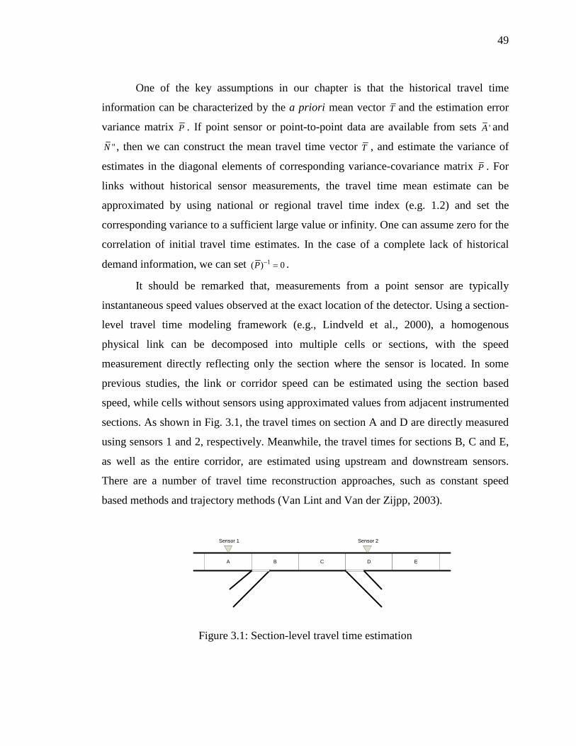
49
One of the key assumptions in our chapter is that the historical travel time
information can be characterized by the a priori mean vector T and the estimation error
variance matrix P . If point sensor or point-to-point data are available from sets 'A and
"N , then we can construct the mean travel time vector T , and estimate the variance of
estimates in the diagonal elements of corresponding variance-covariance matrix P . For
links without historical sensor measurements, the travel time mean estimate can be
approximated by using national or regional travel time index (e.g. 1.2) and set the
corresponding variance to a sufficient large value or infinity. One can assume zero for the
correlation of initial travel time estimates. In the case of a complete lack of historical
demand information, we can set 1( ) 0P − = .
It should be remarked that, measurements from a point sensor are typically
instantaneous speed values observed at the exact location of the detector. Using a section-
level travel time modeling framework (e.g., Lindveld et al., 2000), a homogenous
physical link can be decomposed into multiple cells or sections, with the speed
measurement directly reflecting only the section where the sensor is located. In some
previous studies, the link or corridor speed can be estimated using the section based
speed, while cells without sensors using approximated values from adjacent instrumented
sections. As shown in Fig. 3.1, the travel times on section A and D are directly measured
using sensors 1 and 2, respectively. Meanwhile, the travel times for sections B, C and E,
as well as the entire corridor, are estimated using upstream and downstream sensors.
There are a number of travel time reconstruction approaches, such as constant speed
based methods and trajectory methods (Van Lint and Van der Zijpp, 2003).
A B C D E
Sensor 1 Sensor 2
Figure 3.1: Section-level travel time estimation
50
In this chapter, for sections without point sensors, the above mentioned
approximation error is modeled as prior estimation errors, which can be obtained through
a historical travel time database by considering other related links such as adjacent links
or links with similar characteristics. Furthermore, our proposed framework can be also
easily generalized to a section-based representation scheme, where a section in Fig. 3.1
can be viewed as a link in our link-to-path-oriented modeling structure.
3.3.6 Generic state transition and measurement models
By adapting a structure state model for dynamic OD demand estimation by Zhou
and Mahmassani (2007), this chapter decomposes a true travel time pattern into three
modeling components:
true travel time = regular recurring pattern + structural deviations + random
fluctuations.
Under this assumption, travel time estimation/prediction can be studied in two
categories: recurring traffic conditions and non-recurring conditions. For travel time
prediction under recurring conditions, structural deviation is considered as zero, and the
regular travel time patterns/profiles can be constructed based on historical data for
recurring traffic. On the other hand, for travel time prediction under non-recurring
conditions, the structural deviation is further modelled in this chapter as a function of
time-dependent capacity and time-dependent demand. Without loss of generality, this
chapter mainly focuses on time-dependent capacity reductions due to incidents, a major
source of non-recurring congestion.
To further jointly consider both recurring and non-recurring traffic conditions in
the sensor location problem, the overall system uncertainty under a certain sensor design
is modeled as a probabilistic combination of recurring and non-recurring uncertainty
measures:
overall system prediction uncertainty =
(1 )NRρ− × uncertainty under recurring conditions + NRρ × uncertainty under non-
recurring conditions,
where NRρ represents the given probability of non-recurring events.

51
(i)
The state transition model of the travel time is written as
State transition model
( ) ( ) ( ) , (0, )hd d d d d dT t T t V t w w N Q= + + (1)
In Eq. (1), the travel time for each link is represented as a combination of three
components: regular pattern, structural deviation and random fluctuation. The regular
pattern ( )h
dT t is the time-dependent historical travel time average which is determined by
the day-to-day regular traffic demand and capacity. For non-recurring traffic conditions, a
structural deviation ( )dV t exists due to non-recurring congestion sources such as incidents,
work zones and severe weathers. Considering a stationary congestion pattern, this chapter
assumes that wd follows a normal distribution with zero-mean and a variance-covariance
matrix Qd. Qd corresponds to random travel time variation magnitude, which is further
determined by dynamics and stochasticity in the underlying traffic demand and road
capacity supply. For example, the travel time variations are more significant on a
congested freeway link with close-to-capacity demand flow volume, compared to a rural
highway segment with low traffic volume and sufficient capacity where the speed limit
could yield a good estimate most of the time. More specifically, qd,a , the (diagonal)
variance elements of the matrix Qd, exhibit the travel time variability/uncertainty of each
individual link, while the covariance elements should reveal the spatial correlation
relationship (mostly due to queue spillbacks) between adjacent links in a network. We
refer readers to a chapter by Min and Wynter (2011) for calibrating spatial correlations of
link travel times.
(ii)
In order to estimate the regular pattern
General measurement model
( )h
dT t and structural deviation ( )dV t , a
linear measurement model is constructed as:
( ) ( ) ( )d d d dY t H t T t ε= × + , where (0, )d dN Rε (2)
With the measurement model in Eq. (2), the travel times are estimated using the
latest measurements Yd (t). Measurement vector Yd is composed of travel time
observations from point sensors, point-to-point sensors and probe sensors. The mapping
matrix Hd , with (n × m) elements, connects unknown link travel time Td to measurement

52
data Yd. Particularly, each row in the mapping matrix Hd corresponds to a measurement
and each column corresponds to a physical link in the network. For an element at uth row
and vth column of the matrix Hd , a value of 1 indicates that the uth measurement covers or
includes the travel time on the vth link of the network, otherwise it is 0. With the
measurement equation, the historical recurring travel time pattern is then updated through
the Kalman filtering process.
3.3.7 Uncertainty analysis under recurring and non-recurring conditions
We now focus on the conceptual analysis of the uncertainty reduction and
propagation. By assuming independence between different components in the structure
state model (1), the total variance of the predicted travel time can be obtained by
( ) ( ) ( )var ( ) var ( ) var ( )hd d d dT t T t V t Q= + + (3)
Under recurring congestion conditions, the structural deviation ( ) 0dV t = , which
leads to
( ) ( )var ( ) var ( )hd d dT t T t Q= + .
(4)
To reduce prediction error under recurring conditions, (e.g. at the beginning of
each day d for pre-trip routing applications), we need to reduce the variance of the
historical travel time estimates, ( )var ( )hdT t , while the variance of inherent traffic process
noises Qd (due to traffic demand and supply variations) cannot be reduced and sets a limit
for travel time prediction accuracy. Along this line, this article will first focus on
updating the historical travel time pattern and the uncertainty reduction due to added
sensors under recurring conditions. Under non-recurring conditions, in addition to the
above mentioned uncertainty elements ( )var ( )hdT t and Qd , the total prediction variance is
mainly determined by the structural travel time deviation ( )dV t .
3.4
Focusing on predicting end-to-end path travel time applications and considering
future availability of GPS probe data on links
Conceptual framework and data flow
'''A , the goal of the sensor location problem
is to maximize the overall information gain * arg min ( )l lX z X= by locating point and point-

53
to-point sensors in sets 'A and ''N , subject to budget constraints for installation and
maintenance. To systematically present our key modeling components in the proposed
sensor design model, we will sequentially describe the following three modules.
3.4.1 Link travel time estimation and prediction module
Given prior travel time information dT − and dP−
, with traffic measurement vector
dY that includes ,'d ay , , , ,''d i j ky and ,"'d ay from sensor location sets 'A , ''N and '''A , the link
travel time estimation and prediction module seeks to update current link travel times dT +
and their variance-covariance matrix dP+.
Information quantification module:
With prior knowledge on the link travel time estimates T and P , the information
quantification module aims to find the single-valued information gain ( )lz X for the
critical path travel times for a sensor design scenario lX , represented by location sets 'A , ''N , '''A , as well as AVI and AVL market penetration rates α and β .
3.4.2 Sensor network design module
The sensor design module aims to find the optimal solution * arg min ( )l lX z X= ,
subject to budget constraints for installation and maintenance. For each candidate
solution Xl, this module needs to call the information quantification module to calculate
( )lz X . The optimal solution *X produces optimal location sets 'A and ''N , for a predicted
AVI and AVL market penetration rates α and β, and predicted location set '''A with
reliable travel time map-match results.
Fig. 3.2 illustrates the conceptual framework and data flow for the proposed
modules. From sensor network design plans in block 1, we need to extract three groups of
critical input parameters: AVI/AVL market penetration rates α and β at block 2,
measurement error variance-covariance R in block 3, and sensor location mapping matrix
H in block 4. Location mapping matrix H is derived from the sensor location sets 'A , ''N
and '''A .
54
The link travel time estimation module uses a Kalman filtering model to
iteratively update the travel time (blocks 9 and 10) and the corresponding error variance
matrix (blocks 7 and 8), where the critical Kalman gain matrix K, calculated in block 6, is
applied to the above two mean and variance propagation processes. Based on the
estimation or prediction error variance statistics in blocks 7 and 8, the information
quantification module derives the measure of information in block 11 by representing the
path travel time estimation/prediction quality as a function of P+ and P-. By minimizing
the network-wide path travel time estimation uncertainty, the sensor network design
module finally selects and implements an optimized sensor plan so that point sensor, AVI,
and AVL measurement data in block 13 can be produced from the actual sensor network
illustrated by block 12.
One of the key features offered by the Kalman Filtering model is that although
updating the travel time mean estimates from T −in block 9 to T +
in block 10 requires
sensor measurements Y, the uncertainty propagation calculation from block 7 to 8 (i.e.
updating P+from P−
) does not rely on the actual sensor data, as the uncertainty reduction
formula in block 8 is a function of three major inputs: a priori uncertainty matrix P−,
measurement error range R, and sensor mapping matrix H. In other words, if a
transportation analyst can reasonably prepare the above three input parameters, then
he/she can apply the proposed analytical model to compute the information gain for a
sensor design scenario and further assist the decision-maker to determine where and with
what technologies sensor investments should be made in a traffic network.
3.5
One of the fundamental questions in sensor location problems is which criteria
should be selected to drive the underlying optimization processes. Above travel time
estimation and prediction model offer an analytical model for quantifying the
estimation/prediction error reduction due to additional measurements provided by new
sensors. As the process variance-covariance matrix is assumed to be constant, the travel
time uncertainty measure in this section uses the a posterior estimation error covariance
Measure of information for historical traffic patterns

55
P+ as the basis to evaluate the information gain. A challenging question then is how to
select single-value information measures for a sensor design plan. To this end, we first
examine two commonly used estimation criteria, namely, the mean-square error and
entropy. We then propose total path travel time estimation variance as a new measure of
information for end-to-end trip time prediction applications.
4
Travel Time A posteriori Travel Time Estimate
( )T T K Y HT+ − −= + −
A posteriori Estimate Covariance
( )P I KH P+ −= −
A priori Travel Time Estimate
A priori Estimation
Covariance Matrix
Sensor Location Mapping Matrix
H
Measurement Error Variance-covariance
R
Kalman Gain Matrix
1( )T TP H HP H RK − − −= +
T −
P−
3
1
2
Actual Sensor Network
Sensor Network
Design Plan
Data Flow in Kalman Filtering Data Flow in Sensor Network Design
AVI/GPS Market Penetration Rate
α,β
Measure of Information:
Path Travel Time Estimation/Prediction Quality as Function of
P+ and P-
Point Sensor, AVI, GPS
Measurements Y
Optimized Sensor Design
Plan
Non-recurring Traffic Transition Matrix
L
Travel Time Uncertainty13
11
8
10
7
9
6
2
3
1
12
5
Figure 3.2: Conceptual framework and data flow

56
3.5.1 Trace and entropy
The classic Kalman filter aims to minimize the mean-square error, i.e., the trace
of dP+ . The trace of the variance covariance matrix ( )dtr P+ is the sum of the diagonals of
the matrix, which is equivalent to the total variance of link travel time estimates for all
links:
( ) , , ,1 1cov( , ) var( )
m m
d d a d a d aa a
tr P t t t+
= =
= =∑ ∑ (5)
While the trace does not consider the effects of correlation between travel times
of adjacent links, an alternative measure of information is entropy which is commonly
used in information theory applications. For a discrete variable, Shannon’s original
entropy is defined as the number of ways in which the solution could have arisen. For a
continuously distributed random vector T, on the other hand, the entropy is measured by
(ln ( ))E f T− , where f is the joint density function for vector T. If travel time T in our
chapter is assumed to follow a normal distribution, then its entropy is computed as
1ln(det( ))
2 dPθ ++ , where θ is a constant that depends on the size of T, the total number of
links in our chapter network. The entropy measure is proportional to the log of the
determinant of the covariance matrix. By ignoring the constant θ and the monotonic
logarithm function, we can simplify the entropy-based information measure for the a
posteriori travel time estimate as det( )dP+ . The determinant of the variance covariance
matrix, as a measure of information, is also known as the generalized variance.
Mathematically, the trace and determinant of the variance covariance matrix dP+ can be
calculated from the sum and product, respectively, of the eigenvalues of dP+ . Since the
determinant considers the variance and covariance in the matrix, a smaller determinant is
desirable because this indicates a more accurate estimate.
3.5.2 Total path travel time estimation uncertainty
This chapter proposes a new measure of information to quantify the network-wide
value of information, based on the travel time estimation quality of critical OD/paths.

57
The travel time estimation uncertainty of path k from origin o to destination s can
be calculated from the posterior travel time estimate variance-covariance matrix dP+ :
, , , , , ,( , , ) ; , ( , , )
var( ) 2 cov( , )d o s k d a d a d ba p o s k a b a b p o s k
e t t t∈ < ∈
= + ×∑ ∑,
(6)
where var() and cov() are variance and covariance coefficients in the link travel
time uncertainty matrix, respectively. Compared to trace or entropy based information
measures, the proposed path travel time based measure can better capture the possible
correlation between traffic estimates along a path, with the covariance portion of the
estimation error matrix.
A similar equation can be derived for travel time prediction based uncertainty
measure, using the travel time estimate variance-covariance dP− matrix. For sensor
location decisions that jointly consider recurring and non-recurring conditions, an
integrated uncertainty matrix can be generated from recurring travel time uncertainty P−
and non-recurring structure derivation uncertainty −Σ :
(1 )D incident workzone weather recurring incident incident workzone workzone weather weatherP Pρ ρ ρ ρ ρ ρ− − − − −= − − − × + Σ + Σ + Σ
Weighted by the path flow volume of different origin-destination pairs , ,o s kf , the
overall estimation uncertainty of the network-wide traffic conditions on day d can be
determined from the following equation:
( ), , , , ,, ,
d d o s k o s ko s k
TU e f= ×∑
(7)
The above total path travel time estimation uncertainty measure includes three
important components: (1) the sum of elements in the variance covariance matrix for link
travel time estimates; (2) the sum of the travel time variance for each feasible or critical
path in the network; and (3) weights of path flow volume for different paths. As the path
travel time estimation accuracy (as opposed to individual link travel times) is the ultimate
information quality requirement by commuters traveling on various routes, this measure
of information can capture the high-level monitoring performance of a sensor network. In
relation to the trace and entropy measures, the total path travel time estimation

58
uncertainty can be viewed as a more appropriate indicator for system-wide information
gains.
3.6
The proposed sensor network design model is essentially a special case of the
discrete network design problem, so an integer programming model, shown below, can
be constructed to find the optimal sensor location solution.
Sensor design model and beam search algorithm
Min TU
Subject to
Budget constraint:
' ' '' ''a ia i
x xπ π π× + × ≤∑ ∑ (8)
Sensor mapping matrix constraint:
[ ] [ ]( ),' ' , '' '' , ''' , , 0,1,...,d a i d aH function A x N x d Dγ α β= = = = (9)
D = a sufficiently large day number for measure of information to reach
convergence.
'ax = 1 if a point sensor is installed on link a, 0 otherwise.
''ix =1 if an AVI sensor (point-to-point sensor) is installed on node i, 0 otherwise.
'π , ''π = installation and maintenance costs for point sensors and point-to-point
sensors.
π = total available budget for building or extending the sensor network.
In the above objective function, the overall system uncertainty matrix DP− is
calculated as a probabilistic combination of recurring and non-recurring traffic variances.
Structure derivations from different non-recurring traffic conditions are considered in the
total system uncertainty with corresponding probabilities. For links with sensors, the
structure derivation uncertainty is aggregated and averaged from historical measurements
(e.g. 95% or 2σ for normal distribution). For links without sensor, we will take the
maximum of the structure derivation from limited historical database.

59
dH is determined by the sensor location set ' 'aA x= and '' ''iN x= , randomly
generated link traversing coefficient for GPS probe vehicles ,'''d aγ , and AVI and AVL
market penetration rates α and β.
Essentially, the goal of the above sensor location model is to add sensor
information from spatially distributed measurements to minimize the weighted
uncertainty associated with the path travel time estimates. In this chapter, a branch-and-
bound search procedure can be used to solve the integer programming problem. To
reduce the computational complexity, a beam search heuristic algorithm is implemented
in this chapter.
Given prior information on the link travel time vector and its estimation error
covariance from historical database, the proposed algorithm tries to find the best sensor
location scenario from a set of candidates under particular budget constraints. Based on a
breadth-first node selection mechanism, the beam search algorithm branches from the
nodes level by level. At each level, it keeps only φ promising nodes, and prunes the other
nodes permanently to limit the total number of nodes to be examined. φ is typically
referred to as the beam width, and the total computational time of the beam search
algorithm is proportional to the selected beam width.
3.6.1 Beam search algorithm
Step 1: Initialization
Generate candidate link set LC and candidate node set NC for point and point-to-
point sensors, respectively.
Set the active node list ANL = ∅ . Create the root node u with
'( ) , "( )A u N u= ∅ = ∅ , search level ( ) 0sl u = , where u is search node index. Insert the
root node into ANL.
Step 2: Stopping criterion
Terminate and output the best-feasible solution under one of the following
conditions:
(1) If all of the active nodes in ANL have been visited,
(2) The number of active nodes in memory is exceeded.

60
Step 3: Node generation and evaluation
For each node u at search level sl in ANL, remove it from ANL, and generate
child nodes;
Scan through the candidate sets LC, if a link a is not in A'(u), generate a new child
node v’ where '( ') '( ) , "( ') "( ), ( ') ( ) 1A v A u a N v N u sl v sl u= = = + ;
Scan through the candidate sets NC, if a node i is not in N''(u), generate a new
child node v” where "( ") "( ) , '( ") '( ), ( ") ( ) 1N v N u i A v A u sl v sl u= = = + ;
For each newly generated node v, calculate the objective function through DP− . If
the budget constraint is satisfied for a newly generated node, add it into the ANL.
Step 4: Node filtering
Select φ best nodes from the ANL in the search tree, and go back to Step 2.
In the above beam search algorithm, the total computational time is determined by
the number of nodes to be evaluated, which depends on the beam width φ and the size of
the candidate sensor links/nodes. For each node in the tree search process, the complexity
is determined by the evaluation of the objective function, which can be decomposed into
three major steps: (1) calculating P+ from 1TH R H− , (2) calculating the inverse of the
covariance matrix 1( )P+ − , and (3) calculating the path travel time uncertainty as a function
of DP− . The first step involves two matrix multiplications: 1TH R− and 1( )TH R H− . Because
H is an (n×m) matrix and R is an (n×n) matrix, the first step has a worst-case complexity
of O(m2n), and calculating the inverse of matrix leads to an O(m3) operation if the
Gaussian elimination method is used.
For a large-scale sensor network design application, we can adopt three strategies
to reduce the size of the problem and therefore the computational time. First, one can
focus on critical OD pairs with significant volumes. Second, one can aggregate original
OD demand zones into a set of super zones within a manageable size, with this strategy
being especially suitable for a subarea analysis where many OD zones outside the chapter
area can be consolidated together. Third, we can reduce the size of candidate AVL sensor
nodes and point sensor links in order to decrease the number of search nodes to be
evaluated.
61
3.7
To consider long-term information gains of a sensor network in monitoring the
travel time dynamics, the following discussion aims to derive the steady-state results of
uncertainty reduction associated with a fixed sensor network design plan. Considering
both point and AVL sensors, we first assume constant Q, R and H across different days,
the travel time estimation error covariance updating equation as seen in Eq. (10).
Complex cases for updating historical traffic patterns
1 1( )d d dP I K H P Q− −− −= − + (10)
Under steady state conditions, the travel time estimation error covariance will
achieve a constant state as 1d dP P P− −−= = after a number of updates. By applying the
optimal formulation of Kalman gain K, the steady estimation error covariance P is
rewritten as 1( )T TPH HPH R HP Q−+ = (11)
or 1( ( ) )T TP I PH HPH R H P Q−= − + + (12)
Eq. (12) is known as Algebraic Riccati Equation. When numerically solving this
equation, the steady-state travel time estimation error covariance matrix for a long-term
sensor location problem is obtained.
Fig. 3.3 illustrates a day-by-day time series of the travel time estimation variance.
Due to the presence of system evolution noise Q, the estimation variance always
increases when we make a travel time prediction from day d to day d+1, that is,
d d dP P Q− += + . After receiving traffic measurement available every day, the uncertainty
associated travel time estimates is reduced through ( )d d dP I K H P+ −= − . The uncertainty
reduction and the resulting information gain are very dramatic after the first few days of
sensor deployment. After 5 or 6 days, this zig-zag pattern reaches a stable state when
1d dP P− −−= (corresponding to the upper portion of the time series) and 1d dP P+ +
−=
(corresponding to the lower portion of the time series).
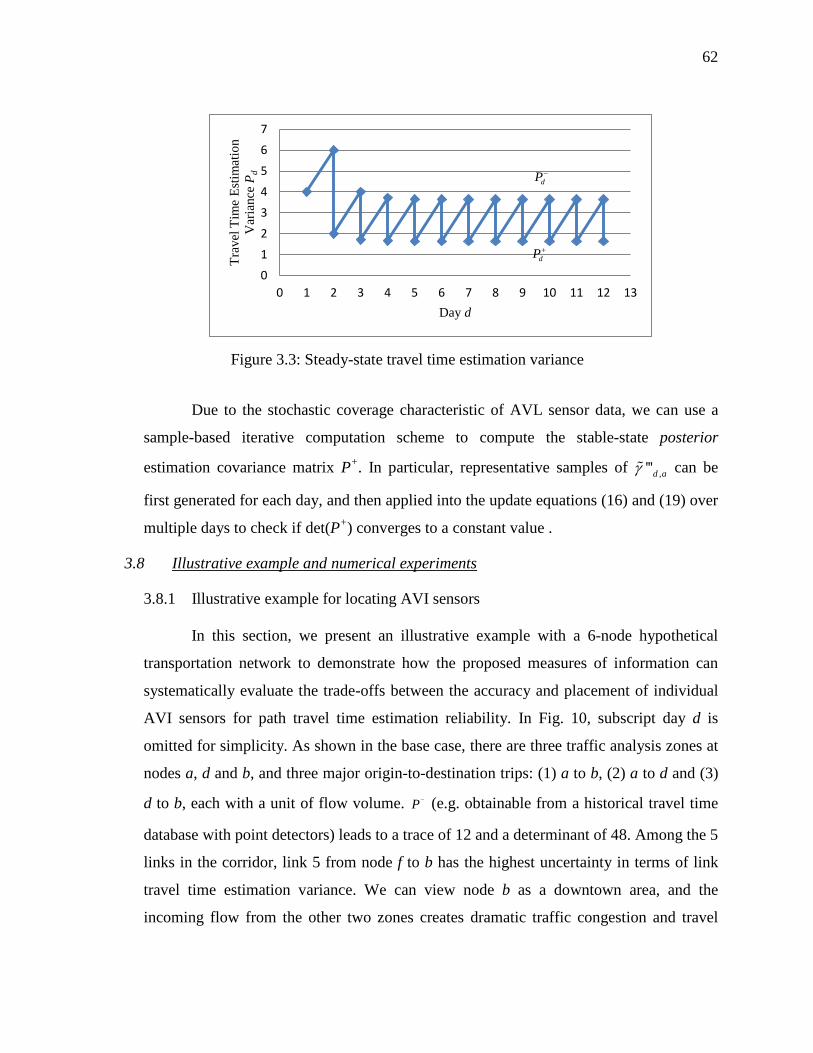
62
Due to the stochastic coverage characteristic of AVL sensor data, we can use a
sample-based iterative computation scheme to compute the stable-state posterior
estimation covariance matrix P+. In particular, representative samples of ,'''d aγ can be
first generated for each day, and then applied into the update equations (16) and (19) over
multiple days to check if det(P+) converges to a constant value .
3.8
3.8.1 Illustrative example for locating AVI sensors
Illustrative example and numerical experiments
In this section, we present an illustrative example with a 6-node hypothetical
transportation network to demonstrate how the proposed measures of information can
systematically evaluate the trade-offs between the accuracy and placement of individual
AVI sensors for path travel time estimation reliability. In Fig. 10, subscript day d is
omitted for simplicity. As shown in the base case, there are three traffic analysis zones at
nodes a, d and b, and three major origin-to-destination trips: (1) a to b, (2) a to d and (3)
d to b, each with a unit of flow volume. P− (e.g. obtainable from a historical travel time
database with point detectors) leads to a trace of 12 and a determinant of 48. Among the 5
links in the corridor, link 5 from node f to b has the highest uncertainty in terms of link
travel time estimation variance. We can view node b as a downtown area, and the
incoming flow from the other two zones creates dramatic traffic congestion and travel
0
1
2
3
4
5
6
7
0 1 2 3 4 5 6 7 8 9 10 11 12 13
Trav
el T
ime
Estim
atio
n V
aria
nce
P d
Day d
Figure 3.3: Steady-state travel time estimation variance
dP−
dP+

63
time uncertainty, first on link 5 and then on link 4. For the base case, we can calculate the
variance of path travel time estimates for these three OD pairs, respectively, as 12, 3 and
9, leading to a total path travel time estimation uncertainty (TU) as TU = 24.
In both cases (I) and (II), two AVI sensors are first installed at nodes a and b. In
case (I), an additional AVI sensor is located at node f so that we can obtain two pairs of
end-to-end travel time measurements: from node a to node f, and from node f to node d.
The second measurement directly monitors travel time dynamics on link 5. In this
particular example along the linear corridor, the end-to-end travel time statistics from a to
b can be explicitly determined from the above two mutually exclusive observations. In
order to avoid double-counting the information gain for the same data sources, the
information quantification module in this chapter only considers two raw measurements:
from a to f, and from f to d, to update the link travel time variance covariance matrix from
P− to P+ . To do so, the measurement error matrix is assumed to be 1 0
0 1
R =
, and
the mapping matrix 1 1 1 1 00 0 0 0 1
H =
, where the first measurement from a to f
covers links 1,2,3 and 4, and the second measurement from f to b covers link 5. As link 5,
with the highest travel time uncertainty, is directly measured from AVI readings, its link
travel time estimate variance is reduced from 4 to 0.8, but the resulting P+ contains a
large amount of correlation in its link travel time estimates for links 1 to 4. All the path
travel time uncertainties for the three OD pairs have been reduced, and TU = 8.5. In case
(II), the third AVI sensor is installed at node d to match the nature OD trip demand
pattern, which produces sensor mapping matrix1 1 0 0 0
0 0 1 1 1
H =
. The resulting
P+ still contains two clusters of correlations corresponding to two individual
measurements from a to d and from d to b. The path travel time estimate variances for the

64
AVI readernode
c d e f1 2 53 4
a bc d e f1 2 53 4
a bc d e f1 2 53 4
Base case
(I) Locate additional AVI reader to reduce highest link travel time uncertainty
(II) Locate additional AVI reader to match origin-to-destination trip pairs
1 0 0 0 00 2 0 0 0
12 48 12 3 9 240 0 2 0 00 0 0 3 00 0 0 0 4
P Tr Det TU−
= = = = + + =
-1
1 0
0 1
1 1 1 1 0 0.89 0.22 0.22 0.33 01 1 1 1 0 0.22 1.56 0.44 0.67 0
1 1 1 1 0 0.22 0.44 1.56 0.67 01 1 1 1 0 0.33 0.67 0.67 2 00 0 0 0 1 0 0 0 0 0.8
6.8 1.07 3.4
T
R
H R H P
Tr Det TU
+
=
− − − − − − = = − − − − − −
= = = 7 2.01 3.02 8.5+ + =
-1
1 0 1 1 0 0 0
0 1 0 0 1 1 1
1 1 0 0 0 0.75 0.5 0 0 01 1 0 0 0 0.5 1 0 0 0
0 0 1 1 1 0 0 1.6 0.6 0.80 0 1 1 1 0 0 0.6 2.1 1.20 0 1 1 1 0 0 0.8 1.2 2.4
7.85 1.2 1.65 0.75
T
R H
H R H P
Tr Det TU
+
= =
− − = = − − − − − −
= = = + + 0.9 3.3=
fk=2 =1fk=1 =1
fk=3 =1
Link 1 2 3 4 5
1 1 1 1 00 0 0 0 1
H =
Measurementa->dd->b
Link 1 2 3 4 5
Measurementa->ff->b
ba
Figure 3.4: Example of locating AVI sensors on a linear corridor
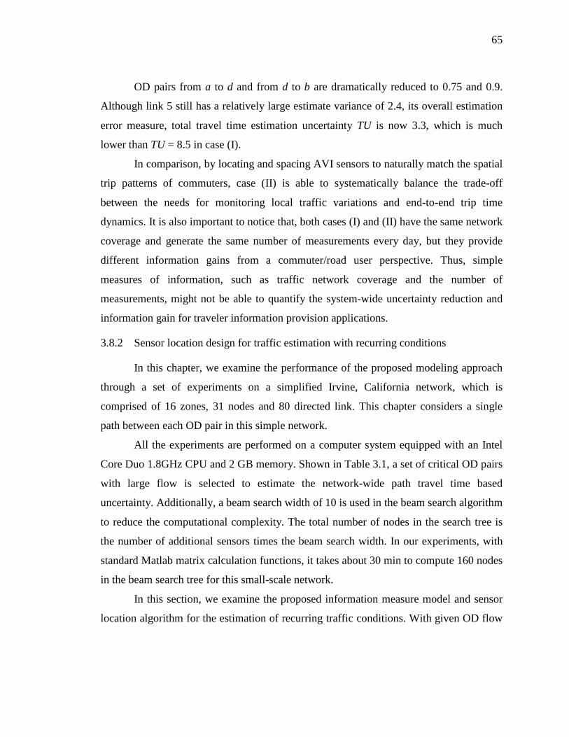
65
OD pairs from a to d and from d to b are dramatically reduced to 0.75 and 0.9.
Although link 5 still has a relatively large estimate variance of 2.4, its overall estimation
error measure, total travel time estimation uncertainty TU is now 3.3, which is much
lower than TU = 8.5 in case (I).
In comparison, by locating and spacing AVI sensors to naturally match the spatial
trip patterns of commuters, case (II) is able to systematically balance the trade-off
between the needs for monitoring local traffic variations and end-to-end trip time
dynamics. It is also important to notice that, both cases (I) and (II) have the same network
coverage and generate the same number of measurements every day, but they provide
different information gains from a commuter/road user perspective. Thus, simple
measures of information, such as traffic network coverage and the number of
measurements, might not be able to quantify the system-wide uncertainty reduction and
information gain for traveler information provision applications.
3.8.2 Sensor location design for traffic estimation with recurring conditions
In this chapter, we examine the performance of the proposed modeling approach
through a set of experiments on a simplified Irvine, California network, which is
comprised of 16 zones, 31 nodes and 80 directed link. This chapter considers a single
path between each OD pair in this simple network.
All the experiments are performed on a computer system equipped with an Intel
Core Duo 1.8GHz CPU and 2 GB memory. Shown in Table 3.1, a set of critical OD pairs
with large flow is selected to estimate the network-wide path travel time based
uncertainty. Additionally, a beam search width of 10 is used in the beam search algorithm
to reduce the computational complexity. The total number of nodes in the search tree is
the number of additional sensors times the beam search width. In our experiments, with
standard Matlab matrix calculation functions, it takes about 30 min to compute 160 nodes
in the beam search tree for this small-scale network.
In this section, we examine the proposed information measure model and sensor
location algorithm for the estimation of recurring traffic conditions. With given OD flow
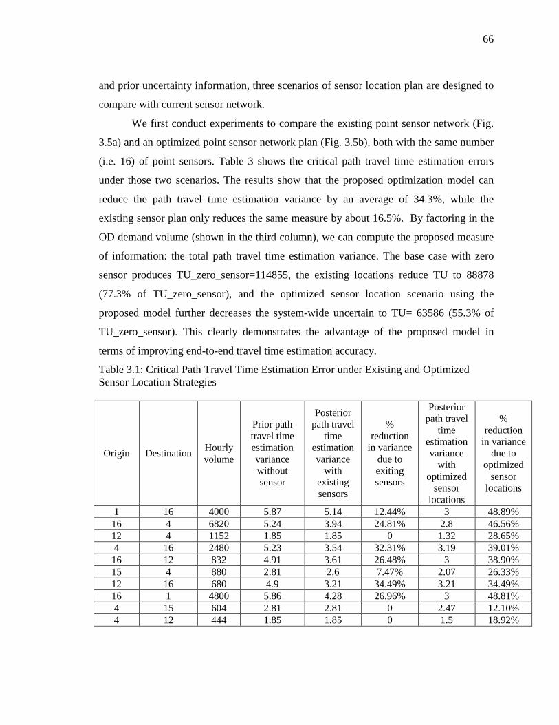
66
and prior uncertainty information, three scenarios of sensor location plan are designed to
compare with current sensor network.
We first conduct experiments to compare the existing point sensor network (Fig.
3.5a) and an optimized point sensor network plan (Fig. 3.5b), both with the same number
(i.e. 16) of point sensors. Table 3 shows the critical path travel time estimation errors
under those two scenarios. The results show that the proposed optimization model can
reduce the path travel time estimation variance by an average of 34.3%, while the
existing sensor plan only reduces the same measure by about 16.5%. By factoring in the
OD demand volume (shown in the third column), we can compute the proposed measure
of information: the total path travel time estimation variance. The base case with zero
sensor produces TU_zero_sensor=114855, the existing locations reduce TU to 88878
(77.3% of TU_zero_sensor), and the optimized sensor location scenario using the
proposed model further decreases the system-wide uncertain to TU= 63586 (55.3% of
TU_zero_sensor). This clearly demonstrates the advantage of the proposed model in
terms of improving end-to-end travel time estimation accuracy.
Table 3.1: Critical Path Travel Time Estimation Error under Existing and Optimized Sensor Location Strategies
Origin Destination Hourly volume
Prior path travel time estimation variance without sensor
Posterior path travel
time estimation variance
with existing sensors
% reduction
in variance due to exiting sensors
Posterior path travel
time estimation variance
with optimized
sensor locations
% reduction
in variance due to
optimized sensor
locations
1 16 4000 5.87 5.14 12.44% 3 48.89% 16 4 6820 5.24 3.94 24.81% 2.8 46.56% 12 4 1152 1.85 1.85 0 1.32 28.65% 4 16 2480 5.23 3.54 32.31% 3.19 39.01%
16 12 832 4.91 3.61 26.48% 3 38.90% 15 4 880 2.81 2.6 7.47% 2.07 26.33% 12 16 680 4.9 3.21 34.49% 3.21 34.49% 16 1 4800 5.86 4.28 26.96% 3 48.81% 4 15 604 2.81 2.81 0 2.47 12.10% 4 12 444 1.85 1.85 0 1.5 18.92%
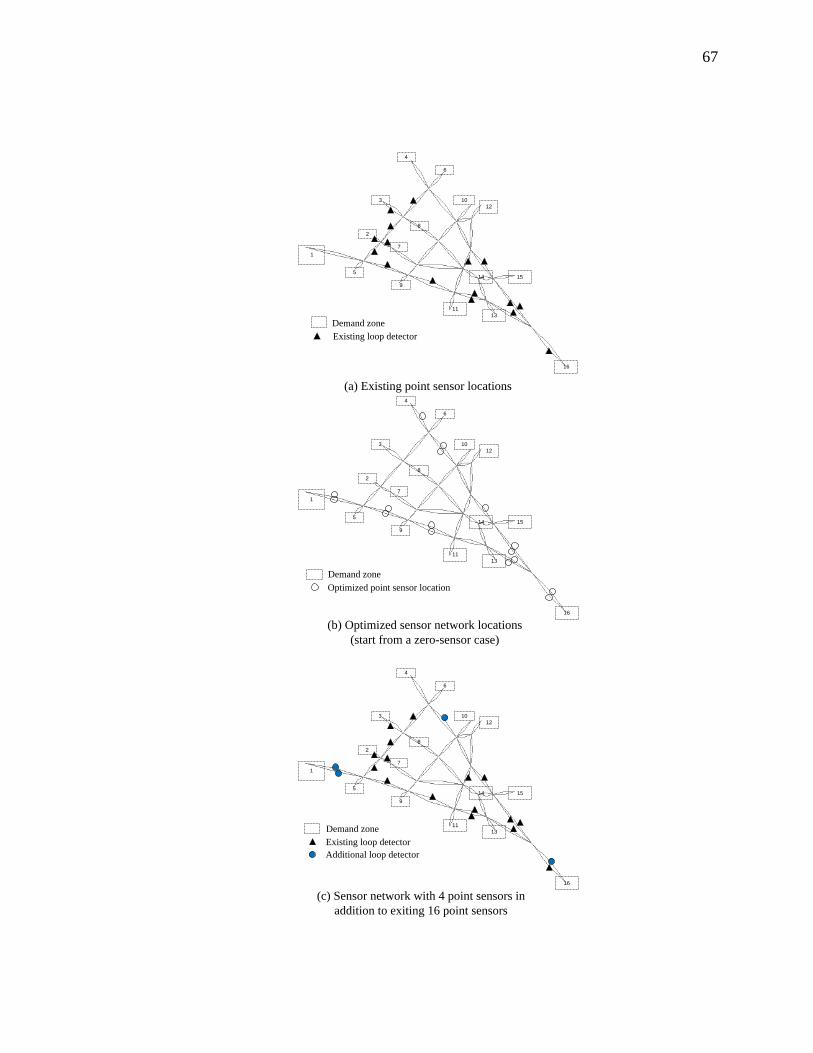
67
1
2
3
4
5
6
7
8
9
1012
1113
14 15
16
Existing loop detectorDemand zone
(a) Existing point sensor locations
1
2
3
4
5
6
7
8
9
1012
1113
14 15
16
(b) Optimized sensor network locations (start from a zero-sensor case)
Optimized point sensor locationDemand zone
1
2
3
4
5
6
7
8
9
1012
1113
14 15
16
Existing loop detectorDemand zone
Additional loop detector
(c) Sensor network with 4 point sensors in addition to exiting 16 point sensors

68
1
2
3
4
5
6
7
8
9
1012
1113
14 15
16
Existing loop detectorDemand zone
Additional AVI sensor
(d) Sensor network with 6 AVI sensors in addition to exiting 16 point sensors
In the next set of numerical experiments, we compare two scenarios with
additional sensors on top of the existing sensors.
1) Add 4 point sensors on uncovered links still with large travel time variance,
leading to a total 16+4=20 point sensors, shown in Fig. 3.5(c);
2) Add 6 AVI readers on major zones with large volume, leading to a network
with 16 point sensors and 6 AVI readers, shown in Fig. 3.5(d).
Fig. 3.6 further compares the measure of uncertainty at different stages. It is
interesting to observe that compared to the optimized scenario (from the scratch) with 16
sensors, this “additional point sensors” scenario (with 20 sensors) does not offer a
superior uncertainty reduction performance for different OD pairs. On the other hand,
compared to adding 4 point sensors to cover highly dynamic links, installing additional 6
AVI sensors does not further improve the path travel time estimation performance
dramatically.
Figure 3.5: Numerical experiment results for regular traffic pattern estimation.

69
3.8.3 Sensor location design for traffic prediction with recurring and non-recurring
conditions
Now we perform the proposed algorithm by considering both regular and non-
recurring traffic conditions. As discussed in Section 7, the total traffic prediction
uncertainty is computed as a probabilistic combination of recurring and non-recurring
uncertainties. In this numerical experiment, we take the incident as a demonstration
example, with the link based incident rates shown in Fig. 3.7(a). The proposed sensor
location algorithm is applied in three scenarios: (1) optimized sensor network with 16
point sensors, (2) current network with additional 4 point sensors, and (3) current
network with additional 6 AVI sensors. Consequentially, these three sensor network
design results are plotted in Figs.3.7(b-d). It is interesting to note that when considering
non-recurring traffic conditions (incidents), the optimized sensor locations (Fig. 13b) are
more focused on links with higher incident rates, compared to the regular pattern
estimation based planning result in Fig. 11(b).
1 2 3 4 5 6 7 8 9 101
1.5
2
2.5
3
3.5
4
4.5
5
5.5
Sequence of Critical OD/Path
Pat
h Tr
avel
Tim
e E
stim
atio
n V
aria
nce
Posterior variance of existing sensorsPosterior variance for optimized sensor networkPosterior variance with additional loop detectorsPosterior variance with additional AVI sensors
Figure 3.6: Comparison of different sensor location schemes (for regular traffic estimation)

70
(a) Annual incident rate
1
2
3
4
5
6
7
8
9
1012
1113
14 15
16
Annual incidents per mileDemand zone
50100150200300
(b) Optimized sensor network locations (start from a zero-sensor case)
1
2
3
4
5
6
7
8
9
1012
1113
14 15
16
Optimized point sensor locationDemand zone
1
2
3
4
5
6
7
8
9
1012
1113
14 15
16
Existing loop detectorDemand zone
Additional loop detector
(c) Sensor network with 4 point sensors in addition to exiting 16 point sensors

71
1
2
3
4
5
6
7
8
9
1012
1113
14 15
16
Existing loop detectorDemand zone
Additional AVI sensor
(d) Sensor network with 6 AVI sensors in addition to exiting 16 point sensors
3.9. Conclusions
To provide effective congestion mitigation strategies, transportation engineers and
planners need to systematically measure and identify both recurring and non-recurring
traffic patterns through a network of sensors. The collected data are further processed and
disseminated for travelers to make smart route and departure decisions. There are a
variety of traditional and emerging traffic monitoring techniques, each with ability to
collect real-time traffic data in different spatial and temporal resolutions. This chapter
proposes a theoretical framework for the heterogeneous sensor network design problem.
In particular, we focus on how to better construct network-wide historical travel time
databases, which need to characterize both mean and estimation uncertainty of end-to-end
path travel time in a regional network.
A unified Kalman filtering based travel time estimation and prediction model is
first proposed in this research to integrate heterogeneous data sources through different
measurement mapping matrices. Specifically, the travel time estimation model starts with
the historical travel time database as prior estimates. Point-to-point sensor data and GPS
probe data are mapped to a sequence of link travel times along the most likely travelled
path. Through an analytical information updating equation derived from Kalman filtering,
the variances of travel times on different links are estimated for possible sensor design
Figure 3.7: Numerical experiment results under recurring and non-recurring traffic conditions

72
solutions with different degree of sampling or measurement errors. The variance of
travel time estimates for spatially distributed links are further assembled to calculate the
overall path travel time estimation uncertainty for the entire network as the single-valued
information measure. The proposed information quantification model and beam search
solution algorithm can assist decision-makers to select and integrate different types of
sensors, as well as to determine how, when, where to integrate them in an existing traffic
sensor infrastructure.
In our on-going research, we plan to expand the research in the following ways.
First, this chapter only focuses on the sensor design problem for estimating the mean of
path travel time, and a natural extension is to assist sensor design decisions for other
network-wide traffic state estimation domains, such as measuring and forecasting point-
to-point travel time reliability, and incident detection probability. Second, under
assumptions of normal distributions for most error terms, the proposed sensor location
model is specifically designed for the minimum path travel time estimation variance
criterion, and our future work should consider other crucial factors for real-world sensor
network design, such as allowing log-normally distributed error terms and minimizing
maximum estimation errors. Furthermore, the offline model developed in this chapter
could be extended to a real-time traffic state estimation and prediction framework with
mobile and agile sensors. The numerical experimental results (for a small-scale network)
in this chapter also demonstrate computational challenges (due to heavy-duty matrix
operations) in applying the proposed information-theoretic sensor location strategy in
large-scale real-world networks, and these challenges call for more future research for
developing efficient heuristic and approximation methods.
73
CHAPTER 4. QUANTIFYING VALUE OF TRAFFIC INFORMATION
Over the past two decades, real-time information systems have been proposed as a
mechanism to generate system-wide and individual travel time savings in congested
vehicular traffic networks. Ideally, a traveler/driver would fully comply with such
information. However, more likely, he/she would use it to partly modify the existing trip
route or completely ignore the information based on inherent behavioral tendencies, past
experience, situational factors (such as time-of-day, weather conditions, and trip
purpose), and the ambient traffic conditions encountered (Peeta and Yu, 2006). Hence,
the complexities associated with driver behavior may impact the reliable prediction of
traffic network states unfolding over time as well as the potential benefits derived from
information provision. Traditionally, the prediction of system performance under real-
time information provision has been studied using dynamic traffic assignment (DTA)
models (Ben-Akiva, et al., 1998; Mahmassani, et al., 1998) in which individuals are
assigned to time-dependent routes from their origins or en-route locations to their
destinations so as to satisfy some system-wide objective and/or individual user level
constraints. However, these models primarily focus on modeling the traffic flow
propagation robustly, while the role of traveler behavior on the evolution of the network
dynamics has largely been subsumed by making potentially restrictive a priori
assumptions on behavior (Peeta and Yu, 2006). For example, such assumptions include
one or more of the following: (i) travel time is the only basis for route choice decision-
making, (ii) users are behaviorally homogeneous, and/or (iii) pre-specified behavior
classes are available whose fractions are known in the ambient traffic stream. Further,
they do not consider learning that takes place over longer timescales.
Several simulation-based studies have been conducted over the past two decades
to analyze the evolution of the traffic network under real-time information provision to
drivers. Some of them assume specific driver behavior models and seek to understand the
effect of real-time information on the unfolding network states. Others combine an
underlying traffic simulator with laboratory-based interactive experiments where the
74
participants are provided real-time routing information on the traffic conditions related to
their origin-destination (O-D) trip. Thereby, their real-time decisions are simulated along
with that of the ambient traffic for the test network (Adler, et al., 1993; Pel, 2011;Kwan et.
al., 2006; Adler and McNally, 1994). However, the various simulation studies are typically
limited by one or more of the following: (i) the need to pre-specify behavior models, (ii)
the small number of participants, and (iii) the type of network topology considered (such
as parallel route corridors). More importantly, and of fundamental relevance to the
proposed work, there is a presumption of the type of information available, how and
when it can be delivered to the individual travelers, and how it is processed by the
travelers. In simulations models, all of these are seamless and the focus is purely on the
estimating the potential benefits of real-time information provision. Unfortunately, this is
where there is an underlying disconnect with the real-world, beyond the key issues
related to restrictive behavioral assumptions. First, travelers can process only limited
information while driving. Hence, it is important to characterize the effects of real-time
information based on providing only information that can be realistically processed by
individuals in real-time (as opposed to unstated assumptions in simulation models of the
ability to process any information provided). Second, due to safety concerns and the
inability of individuals to multitask safely while driving, how the information is provided
to them (for example, voice, visual, or text) becomes a key issue. Again, this is presumed
as seamless in simulation models. Third, there are technological issues related to when
information is provided to travelers. This would imply the continuous tracking of each
traveler or mechanisms for two-way communication with an automated server. That is,
how would the information system operator ensure the timeliness of the information
provided to a traveler relative to his/her current location in the network? In simulation
models, there is an implicit assumption that a traveler can be accessed anywhere, or
possibly at discrete points, in the network to provide such information. Hence, even if we
were to discount issues related to the adequacy of representing traveler behavior, the
three issues mentioned heretofore would lead to gaps between the benefits predicted by a
simulation model and those of actual field experiments.

75
To provide a better understanding of the potential value of real-time traffic
information to travelers, we propose carefully designed field experiments that
additionally seek to explicitly capture the behavioral aspects of travelers. That is, we seek
to analyze the effect of the actual information provided to a traveler on that traveler’s
response after each instance of such information provision. The collected data will be
used to develop more reliable models of traveler response behavior by identifying the
various factors that affect decision-making under information provision. Further the
experiments will help in identifying additional performance measures beyond the
traditionally used benchmark of travel time savings that leads to better understanding of
the potential benefits of a real-time information system to both the user and the operator.
4.1
The proposed chapter seeks to determine the value of real-time information for
travelers through carefully designed field experiments that circumvent the limitations of
computer simulations as well as the methodological challenges. The experiments will be
conducted using a sample of 500 participants in Indianapolis city by tracking their daily
morning commute (from home to work) under pre-trip and en-route real-time information
provided via the Internet and GPS-enabled cell phones. The chapter will first create a
diverse pool of volunteer participants for the experiment. They will be chosen so as to
represent the general driving population, and will be additionally filtered based on their
access to the relevant technology (GPS-enabled cell phones or Smartphones and
Internet). As a participant’s home-to-work commute will be tracked for each day of the
experiment, they will be provided a privacy compliance letter. Once the participants have
qualified for the survey, they will be given login information to the chapter website and
an app to install on their cellphones. Each participant will have a separate database which
will be stored in the server.
Field Experiment
As a pre-processing step, the participants will be required to provide their usual
routes from home to work, familiarity with routes, attitude towards information, and
other socio-economic characteristics in a one-time online survey. Next, for each day of
76
the duration of the experiment, each participant fills a daily trip diary about their actions
related to the real-time information provided after the trip; these will be supplemented
using GPS-based tracking data for that participant. The experiments will be conducted
only for the home-to-work commute so as to maintain data consistency and enhance the
ability of participants to retain memory while filling the daily trip diary. The one-time
online survey and the daily trip diary will provide data to capture the qualitative
behavioral aspects of the response towards the supplied real-time information. The
quantifiable aspects will be in form of the potential travel time savings obtained by
changing the current route at each instance. A combination of the stated and revealed
preference data will be used to derive the quantitative and qualitative value of the real-
time information to the customers.
4.2
The advent of modern real-time traffic information dissemination technologies
and potential future levels of market penetration make it technologically viable to send
personalized information in both pre-trip and en-route contexts (to smart phones through
websites like traffic.com, GPS Navigation system through traffic receivers), as well as
generic information en-route (through variable message signs (VMS)) and pre-trip
(through traffic information websites and radio FM). Further, technologically, it is
possible to track the compliance, non-compliance or partial compliance related to the
information provided using devices such as GPS (Lawson et al., 2008), supplemented
further manually by travelers’ daily trip diaries (Asakura and Hato, 2004; Itsubo and
Hato, 2006). Nevertheless, significant methodological challenges exist beyond privacy
concerns in enabling related field studies. First, to understand an individual traveler’s
response, there is the need to obtain data on his/her inherent behavioral tendencies (for
example, the level of willingness to take risks) as well as attitude towards information
provided. Second, the ability to understand whether information provision at any point in
time caused the traveler to shift from his/her current route requires the knowledge of the
current route at each information provision time instance as well as the commonly-used
routes by that traveler for the daily commute. Third, ideally, the decision of the traveler is
Data Availability
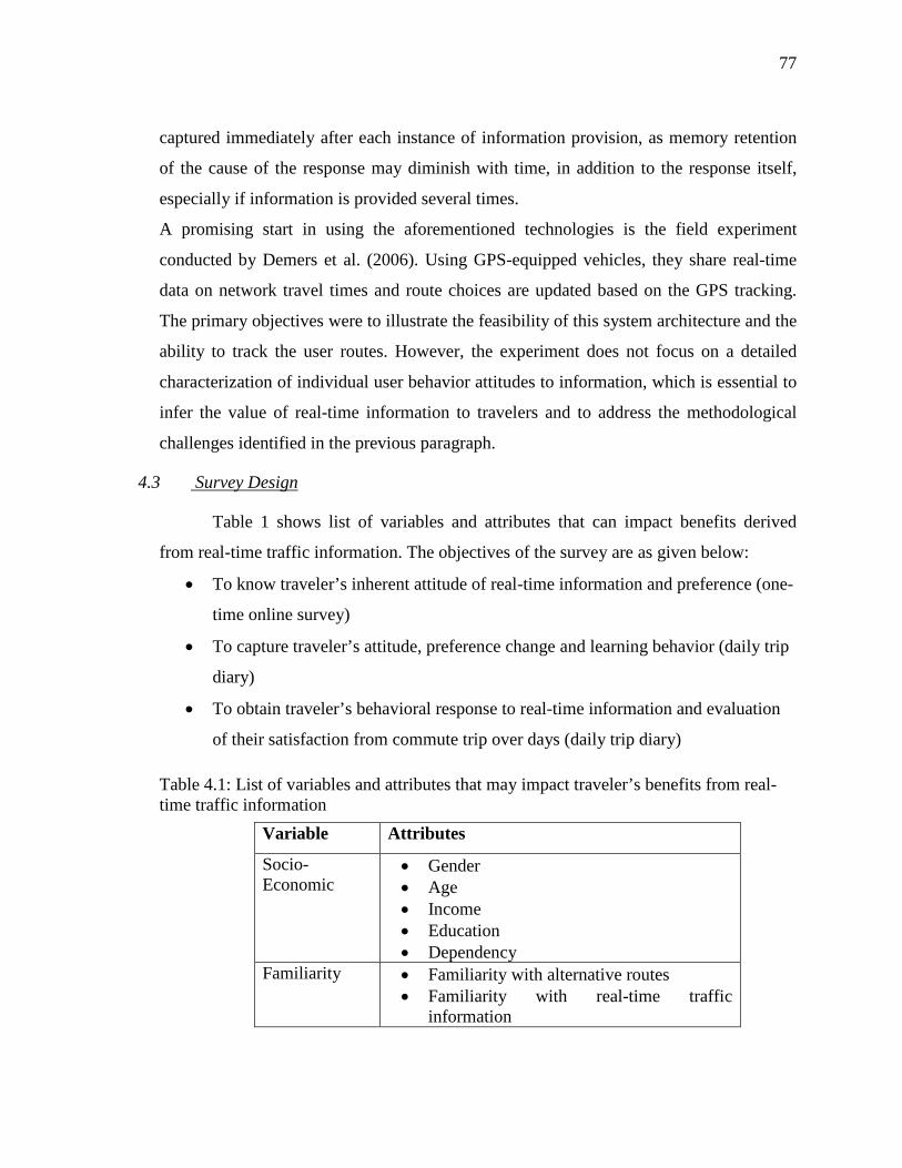
77
captured immediately after each instance of information provision, as memory retention
of the cause of the response may diminish with time, in addition to the response itself,
especially if information is provided several times.
A promising start in using the aforementioned technologies is the field experiment
conducted by Demers et al. (2006). Using GPS-equipped vehicles, they share real-time
data on network travel times and route choices are updated based on the GPS tracking.
The primary objectives were to illustrate the feasibility of this system architecture and the
ability to track the user routes. However, the experiment does not focus on a detailed
characterization of individual user behavior attitudes to information, which is essential to
infer the value of real-time information to travelers and to address the methodological
challenges identified in the previous paragraph.
4.3
Table 1 shows list of variables and attributes that can impact benefits derived
from real-time traffic information. The objectives of the survey are as given below:
Survey Design
• To know traveler’s inherent attitude of real-time information and preference (one-
time online survey)
• To capture traveler’s attitude, preference change and learning behavior (daily trip
diary)
• To obtain traveler’s behavioral response to real-time information and evaluation
of their satisfaction from commute trip over days (daily trip diary)
Table 4.1: List of variables and attributes that may impact traveler’s benefits from real-time traffic information
Variable Attributes
Socio-Economic
• Gender • Age • Income • Education • Dependency
Familiarity • Familiarity with alternative routes • Familiarity with real-time traffic
information
78
Situational • Congestion • Incident • Adverse Weather • Construction • Time of the day
4.4
For each day of the field experiment, before leaving for their commute, participants
access the study website or customized app installed on their cell phones to obtain: (i)
current traffic conditions, and (ii) projected traffic conditions on their routes. The current
traffic conditions will be based on the real-time traffic information available from the
traffic feed from NAVTEQ (owner of traffic.com). NAVTEQ provides real-time traffic
information from four types of sources: digital traffic sensors, GPS/probe devices,
commercial and government partners, and its own traffic operations center staff
members. Also, a dedicated staff at traffic operations centers for each of the cities
consistently monitors traffic conditions. NAVTEQ also maintains historical traffic
patterns (a database with information about the average traffic speed for specific sections
of roadways, geo-referenced to the NAVTEQ map).The projected traffic conditions will
be based on the expected traffic at different time intervals on the routes based on traffic
history and real-time information using advanced predictive algorithms.
Experimental Design
The participant will choose the route he/she wishes to follow for that day and records it
on the study website or cell phone app. Once the participant starts his/her trip, his/her
location will be tracked using the GPS-enabled cell phone by two way communication
from the server. The app installed in a cell phone tracks real-time locations, speeds, and
headings of participants in the vehicle, and communicate this information to the server. If
required, he/she can disable the app after each trip. During the home-to-work trip, the
participant will be provided en-route traffic updates based on the changes in the traffic
conditions on the chosen route and their response is tracked. After finishing the trip on a
specific day, the participant fills the daily trip diary which will have queries regarding the
information provided and their experience with the information in qualitative terms (type
of information received, reliability of the information, the reason for the choosing/not

79
choosing the prescribed route, and level of satisfaction based on information (on Likert
scale)). This process is repeated for each day of the planned field experiment i.e. atleast
30 days.
After finishing the field experiment, the next step is to check for the consistency of the
recorded trip diaries. If the trip route data is inconsistent with the tracked information, the
tracked information is used for analysis. The next step is to analyze whether a participant
followed the usual route or the route suggested by the real-time information. The stored
data in the server will be used for analysis. The quantitative benefits will be calculated as
the difference between the actual travel time had the participant followed the pre-
trip/current route and the travel time if he/she followed the suggested route. The
qualitative benefits will be measured using user feedback on the perceived usefulness of
traffic information, level of satisfaction, and reduction in anxiety. Using a large portion of
the finalized study data, econometric and statistical analysis will be performed to
characterize the quantifiable and qualitative benefits of real-time information. The
analyses will be used to construct reliable models of traveler response behavior under
real-time information.
4.5
The goal of this study is to measure and understand the benefits of real-time
traffic information to the commuter by investigating the physical and psychological
benefits of real-time information by developing reliable traveler behavior models that can
be used to predict costs and benefits for real-world deployment. Two key aspects of this
study are: (i) the proposed field experiments seek to develop robust behavior models
related to real-time information provision that can be used reliably in practice, and (ii) the
study seeks to identify performance measures beyond just the travel time savings to
understand the value of a real-time information system for the user and operator. The
expected results are better understanding of psychological benefits to users from real-
time traffic information beyond travel time savings. We will also be able to explore if
mere availability of information gives assurance to the user irrespective of quality of
information in an unfamiliar location.
Concluding comments
80
CHAPTER 5. CONCLUSIONS AND FUTURE RESEARCH
5.1
In this study three major objectives were identified to be accomplished to exploit
innovative data collection, traffic management, and road pricing/crediting mechanisms
that can encourage mutually beneficial information-sharing under innovative partnerships
for real-time traffic information systems. The first objective was to develop a unified data
mining system that can synthesize different data sources to estimate traffic network
states. Second, we identified existing deficiencies in data quality, coverage and reliability
in an existing DOT traffic sensor network and develop an information gain theoretic
model for optimal sensor location that can take into account uncertainty. The third
objective was to measure and understand the physical and psychological benefits of real-
time traffic information to the commuters and develop reliable traveler behavior models
that can be used to predict costs and benefits for deployment of such systems to
stakeholders. Each of these objectives has been studied in separate chapters in the study.
Summary
In the second chapter we investigated cumulative flow count-based system
modeling methods that estimate macroscopic and microscopic traffic states with
heterogeneous data sources on a freeway segment. A novel approach of use of the
multinomial probit model and Clark’s approximation method is used to develop a
stochastic three-detector model. The model estimates the mean and variance-covariance
of cumulative vehicle counts on both ends of a traffic segment, which are used as
probabilistic inputs for estimating cell-based flow and density inside the space-time
boundary and to construct a series of linear measurement equations within a Kalman

81
filtering estimation framework. This research presented an information-theoretic
approach to quantify the value of heterogeneous traffic measurements for specific fixed
sensor location plans and market penetration rates of Bluetooth or GPS flow car data.
In the next chapter, we study the second objective, where an information-theoretic
sensor location model that aims to maximize information gains from a set of point, point-
to-point and probe sensors in a traffic network is proposed. This model gives a particular
emphasis on the end-to-end travel time prediction problem. Based on a Kalman filtering
structure, the proposed measurement and information quantification models explicitly
take into account several important sources of errors in the travel time
estimation/prediction process, such as the uncertainty associated with prior travel time
estimates, measurement errors and sampling errors. Further, a discussion on quantifying
information gain for steady state historical databases and point-to-point sensors with
multiple paths is provided. A heuristic beam-search algorithm is developed to solve the
proposed combinatorial sensor selection problem. A number of illustrative examples are
used to demonstrate the effectiveness of the proposed methodology.
The fourth chapter aims to study the benefits of real-time traffic information
systems to the commuter by investigating the physical and psychological benefits of real-
time information by developing reliable traveler behavior models that can be used to
predict costs and benefits for real-world deployment of these systems. The study
proposes field experiments to develop robust behavior models related to real-time
information provision that can be used reliably in practice. Further, the study seeks to
identify performance measures beyond just the travel time savings to understand the
value of a real-time information system for the user and operator. The proposed
experiment is yet to be performed, but the survey design and experiment plan has been
discussed in detail in the chapter.
5.2
There are several potential future research directions. As mentioned earlier, this is the
first year report of a multiple year effort. Future research will focus on the following
major aspects:
Future research directions
82
(i) The proposed single-segment-oriented methodology will be further extended
for a corridor model with merges/diverges for possible medium-scale traffic
state estimation applications.
(ii) The proposed model for the traffic state estimation problem will be further
extended to a real-time recursive traffic state estimation and prediction
framework involving multiple O-D pairs with stochastic demand patterns or
road capacities.
(iii) Given the microscopic state estimation results, one can quantify the
uncertainty of other quantities in many emerging transportation applications,
e.g., fuel consumption and emissions that mainly dependent on cell-based or
vehicle-based speed and acceleration measures, and link-based travel times
that can be related to the cumulative vehicle counts on the boundary.
(iv) This study only focuses on the sensor design problem for estimating the mean
of path travel time, and a natural extension is to assist sensor design decisions
for other network-wide traffic state estimation domains, such as measuring
and forecasting point-to-point travel time reliability, and incident detection
probability.
(v) The proposed sensor location model is specifically designed for the minimum
path travel time estimation variance criterion with assumptions of normal
distributions for most error terms. The future work should consider other
crucial factors for real-world sensor network design, such as allowing log-
normally distributed error terms and minimizing maximum estimation errors.
(vi) Furthermore, the offline model developed in this study could be extended to a
real-time traffic state estimation and prediction framework with mobile and
agile sensors.
(vii) The proposed field experiments for real-time traffic information need to be
performed to gain insights into the quantification of real-time traffic
information benefits.
83
REFERENCES
1) Ashok, K., Ben-Akiva, M.E., 2000. Alternative approaches for real-time estimation and prediction of time-dependent origin-destination flows. Transportation Science 34(1), 21-36.
2) Ashok, K., 1996. Estimation and Prediction of Time-Dependent Origin-Destination Flows, Ph.D. Dissertation, MIT. 143-149.
3) Cassidy, M., Coifman, B., 1997, Relation among average speed, flow, and
density and the analogous relation between density and occupancy, Transportation Research Record 1591, 1-6.
4) Clark, C. E., 1961. The greatest of a finite set of random variables. Operations Research 9(2), 145-162.
5) Coifman, B., 2002. Estimating travel times and vehicle trajectories on freeways using dual loop detectors. Transportation Research Part A 36(4), 351-364.
6) Daganzo, C.F., Bouthelier F., Sheffi, Y., 1977. Multinomial probit and Qualitative Choice: A Computationally Efficient Algorithm. Transportation Science 11(4), 338-358.
7) Daganzo, C. F., 1979. Multinomial probit: The theory and its application to demand forecasting. Academic Press, New York. 118-125.
8) Daganzo, C. F., 1994. The cell transmission model: a dynamic representation of highway traffic consistent with the hydrodynamic theory. Transportation Research Part B 28(4), 269-287.
9) Daganzo, C. F., 1997. Fundamental of transportation and traffic operations. Pergamon, Oxford, UK.
10) Daganzo, C. F., 2003. A variational formulation of kinematic waves: solution methods. Transportation Research Part B 39(10), 934-950.
11) Daganzo, C. F., 2005. A variational formulation of kinematic waves: basic theory and complex boundary conditions. Transportation Research Part B 39(2), 187-196.

84
12) Daganzo, C. F., 2006. In traffic flow, cellular automata=kinematic waves. Transportation Research Part B, 40(5), 396-403.
13) FHWA., 2008. The next generation simulation (NGSIM). URL: http://www.ngsim.fhwa.dot.gov.
14) Haghani, A., Hamedi, M., Sadabadi, K. F., Young, S., Tarnoff, P., 2010. Data collection of freeway travel time ground truth with Bluetooth sensors. Transportation Research Record, 2160, 60-68.
15) Herrera, J. C., Bayen, A. M., 2010. Incorporation of Lagrangian measurements in freeway traffic state estimation. Transportation Research Part B 44(4), 269-287.
16) Horowitz, J.L., Sparmann, J. M., Daganzo, C. F., 1982. Investigation of accuracy of Clark approximation for multinomial probit Model. Transportation Science 16(3), 382-401.
17) Hurdle, V. F., Son, B., 2000. Road test of a freeway model. Transportation Research Part A 34(7), 537-564.
18) Hurdle, V. F., Son, B., 2001. Shock wave and cumulative arrival and departure models: Partners without conflict. Transportation Research Record 1176, 159-166.
19) Kim, T., Zhang, H., 2008. A stochastic wave propagation model. Transportation Research Part B, 42(7-8), 619-634.
20) Lighthill, M.J., Whitham, G.B., 1955. On kinematic waves: II. A theory of traffic flow on long crowded roads, In: Proc. Royal Society, vol. 229 (1178) of A, pp. 317–345.
21) Mehran, B., Kuwahara. M., Naznin, F., 2011, Implementing kinematic wave theory to reconstruct vehicle trajectories from fixed and probe sensor data. Proceeding of the 19th International Symposium on Transportation and Traffic Theory, Berkeley , USA, vol.17, pp. 247-268.
22) Mihaylova, L., Boel, R., Hegyi, A., 2007. Freeway traffic estimation within particle filtering framework. Automatica 43 (2), 290–300.
23) Muñoz, L., Sun, X., Horowitz, R., Alvarez, L., 2003. Traffic density estimation with the cell transmission model. In: proceedings of the American control conference. Denver, Colorado, USA, pp. 3750-3755.
24) Nanthawichit, C., Nakatsuji, T., Suzuki, H., 2003. Application of probe-vehicle data for real-time traffic-state estimation and short-term travel-time prediction on a freeway. Transportation Research Record 1855, 49-59.
25) Newell, G. F., 1993. A simplified theory of kinematic waves in highway traffic, part I: General Theory. Transportation Research Part B 27(4), 281-297.

85
26) Newell, G. F., 2002. A simplified car-following theory: a lower order model. Transportation Research Part B, 36(3), 195-205.
27) Richards, P.I., 1956. Shock waves on the highway. Operations Research 4(1), 42–51.
28) Sheffi, Y., 1985. Urban transportation networks. NJ, USA: Prentice-Hall. 379-380.
29) Son, B., 1996. A chapter of G.F.Newell’s “simplified theory of kinematic waves in highway traffic.” Ph.D. Dissertation, University of Toronto, Canada.
30) Sumalee, A., Zhong, X., Pan, L., Szeto, Y., 2011. Stochastic cell transmission model (SCTM): A stochastic dynamic traffic model for traffic state surveillance and assignment. Transportation Research Part B 45(3), 507-533.
31) Sun, X., Muñoz, L., Horowitz, R., 2003. Highway traffic state estimation using improved mixture Kalman filters for effective ramp metering control. In: Proceedings of the 42nd IEEE Conference on Decision and Control. Hawaii, USA, 6333–6338.
32) Treiber, M., Helbing, D., 2002. Reconstructing the spatio-temporal traffic dynamics from stationary detector data. Cooper@tive Tr@nsport@tion Dyn@mics 1, 3.1–3.24.
33) Xing, T., Zhou, X., 2011, Designing Heterogeneous Sensor Networks for Estimating and Predicting Path Travel Time Dynamics: An Information-Theoretic Modeling Approach. Submitted to Transportation Research Part B.
34) Wang, Y., Papageorgiou, M., 2005. Real-time freeway traffic state estimation based on extended Kalman filter: a general approach. Transportation Research Part B 39(2), 141-167.
35) Wang, Y., Papageorgiou, M., Messmer, A., 2007. Real-time freeway traffic state estimation based on extended Kalman filter. Transportation Science 41(2),167-181.
36) Wasson, J.S., Sturdevant, J.R., Bullock, D.M., 2008. Real-time travel time estimates using MAC address matching. Institute of Transportation Engineers Journal, 78(6), 20-23.
37) Work, D. B., Blandin, S., Tossavainen, O.-P., Piccoli, B., Bayen, A. M., 2010. A traffic model for velocity data assimilation. Appl. Math. Res. Express 2010(1), 1-35.
38) Zhou, X., List, G. F., 2010. An information-theoretic sensor location model for traffic origin-destination demand estimation applications. Transportation Science 44(2), 254-273.
39) Zhou, X., Mahmassani, H., 2006. Dynamic OD demand estimation using automatic vehicle identification data. IEEE Transactions on Intelligent Transportation Systems 7(1), 105- 114.

86
40) ABI Research, 2010, http://www.abiresearch.com/home.jsp last accessed on 12th February, 2011.
41) Cellular News, 2010, http://www.cellular-news.com/ last accessed on 12th,
February 2011. 42) NEXTRANS, 2008 “Network Origin-Destination Demand Estimation using
Limited Link Traffic Counts: Strategic Deployment of Vehicle Detectors through an Integrated Corridor Management Framework” Project Report
URL:
http://www.purdue.edu/discoverypark/nextrans/research/completed_projects.php
43) Peeta, S, Yu, J-W., 2006. “Behavior-based consistency-seeking models as deployment alternatives to dynamic traffic assignment models.” Transportation Research Part C, Vol. 14, pp. 114–138.
44) Ben-Akiva, M. Bierlaire, M., Koutsopoulos, H. N., and Mishalani, R., 1998. “DynaMIT: A Simulation based System for Traffic Prediction and Guidance Generation” Proceeding of the 3rd Triennial Symposium on Transportation Systems, San Juan, Puerto Rico.
45) Mahmassani, H.S., Chiu, Y.-C., Chang, G.L., Peeta, S. and Ziliaskopoulous, A.,
1998. “Off-line Laboratory Test Results for the Dynasmart-X Real-Time Dynamic Traffic Assignment System.” Techincal Report ST067-85-TASK-G, Center for Transportation Research, The University of Texas at Austin.
46) Adler, Jeffrey L., Recker, Wilfred W., McNally, Michael G., 1993. “A conflict
model and interactive simulator (FASTCARS) for predicting enroute driver behavior in response to real-time traffic condition information” Transportation Vol. 20 (2) pp. 83 – 106.
47) Pel, Adam J., 2011. “A review on travel behaviour modelling in dynamic traffic
simulation models for evacuations”. Transportation (In press)
48) Kwan, Mei-Po, Casas, Irene, 2006. “GABRIEL: Gis Activity-Based tRavel sImuLator. Activity Scheduling in the Presence of Real-Time Information” GeoInformatica Vol 10 (4) pp. 469-493.
49) Adler, Jeffrey L., McNally, Michael G. 1994. “In-laboratory experiments to
investigate driver behavior under advanced traveler information systems”, Transportation Research Part C: Emerging Technologies, Vol. 2 (3), pp. 149-164.

87
50) Lawson, Catherine T., Chen, Cynthia, Gong, Hongmian, Karthikeyan, Sowmya, 2008. “GPS Pilot Project Phase Three: Mixed Mode Data Collection And Identification Of Special Population Segment” URL :www.nymtc.org/project/surveys/GPS/061508GPS_PILOT_PIII.pdf
51) Asakura, Yasuo, Hato, Eiji., 2004. “Tracking survey for individual travel
behaviour using mobile communication instruments.” Transportation Research Part C Vol. 12 pp. 273–291.
52) Itsubo, Shinji, Hato, Eiji., 2006. “A study of the effectiveness of a household
travel survey using GPS-equipped cell phones and a WEB diary through a comparative study with a paper based travel survey” In CD Proceedings Transportation Research Board 85th Annual Meeting, January 2006.
53) Demers, A., List, G. F., Wallace, W. A., Lee, E. E. and Wojtowicz, J. M., 2006.
“Probes as Path Seekers: A New Paradigm” Transportation Research Record: Journal of the Transportation Research Board, Vol. 1944, pp. 107–114.