DEVELOPMENT OF ACOUSTIC

ANALYSIS TECHNIQUES FOR USE IN

DIAGNOSIS OF VOCAL PATHOLOGY

by

Peter Murphy, BSc.,

Presented to the Office o f Academic Affairs in partial fulfilment o f the thesis

requirements for the degree o f Doctor o f Philosophy in the School o f Physical

Sciences, Dublin City University, Dublin 9

September, 1997

Under the supervision o f :

Professor Martin Henry,

School o f Physical Sciences,

Dublin City University,

Dublin 9

Dr. Kevin McGuigan,

Department of Physics,

Royal College o f Surgeons in Ireland,

123 St. Stephen’s Green,

Dublin 2

(Single Volume)

D e d i c a t e d to m y l a t e f a t h e r , a n d t o m y m o th e r .

I hereby certify that this material, which I now submit for assessment on the

programme of study leading to the award of Doctor o f Philosophy (Ph.D.) is entirely

my own work and has not been taken from the work o f others save and as to the extent

that such work has been cited and Acknowledged within the text o f my work.

Signed: i u j - ID No.

Date: 2 / ( £ } £ $ '?

I

Acknowledgements

I would like to thank Professor Martin Henry for accepting the responsibility o f being

my external supervisor. I would like to express my gratitude to Dr. Kevin M'Guigan,

whose door was always open, for efficiently correcting the thesis and for

encouragement offered throughout the course o f the work.

I would like to express my gratitude to Professor Michael Walsh and Dr. Michael

Colreavy in the ENT department and to Yvonne Fitzmaurice, Antonio Hussey and

Jenny Robinson in the speech therapy department in Beaumont hospital. Thanks also

to Mary Buckley and Patricia Gillivan-Murphy in the Eye and Ear Hospital.

In what, for me, has been a mini-odyssey about the college 1 am left with a lot of

people to show my gratitude. Firstly, I can’t thank enough, everybody up in pathology

and microbiology (Maura, Bemie, Christina, Michael, Dorothy, Doreen, Peadar, Tina,

Ann, Jemma, Brida, and others) who took me under their wing in my first year, when

lumbered with me up in the pathology museum.

Thanks to Julie Duncan and Karen Pierce in physics, both o f whom have been very

helpful to me over the last few years and many thanks also, to Orla Cooney,

particularly in respect to the collaborative time spent together on the present project

before literally taking to the alcohol.

In chemistry I would like to express my gratitude to Eimear O’ Brien, Fiona Bohan,

Joe Jolley, Gillian McMahon, Marie Hosie, Terry Murphy and Karen Lenehan.

Thanks also to all the old school o f Jocelline Levillan, Sylvie Le Roi, Elizabeth

Flannagan, Sharon Brady, Andy Finnucane, Colm Campbell, Adolpho Aquilar,

Suzanne Atkinson, Ali Akbar, Michael Foley, Michaela Walshe and to everyone in the

department.

II

I would also like to thank Chris Murphy for saving me hours o f turmoil with word

processing. Thanks to A.T. Bates for many gifts and to Joanne Fenlon and Ferruccio

Renzoni for providing distractions.

Finally, I wish to thank everyone in the college for making what has been an

exceptionally friendly working environment.

PS Many thanks to everyone in media services for all your help over the past few years.

Ill

Abstract

Acoustic analysis as used in the vocal pathology literature has come to mean any

spectrum or waveform measurement taken from the digitised speech signal. The

purpose o f the work as set out in the present thesis is to investigate the currently

available acoustic measures, to test their validity and to introduce new measures. More

specifically, pitch extraction techniques and perturbation measures have been tested,

several harmonic to noise ratio techniques have been implemented and thoroughly

investigated (three o f which are new) and cepstral and other spectral measures have

been examined. Also, ratios relevant to voice source characteristics and perceptual

correlation have been considered in addition to the tradition harmonic to noise ratios. A

study o f these approaches has revealed that many measurement problems arise and that

the separation of the indices into independent measures is not a simple issue. The most

commonly used acoustic measures for diagnosis o f vocal pathology are jitter, shimmer

and the harmonic to noise ratio. However, several researchers have shown that these

measures are not independent and therefore may give ambiguous information. For

example, the addition o f random noise causes increased jitter measurements and the

introduction o f jitter causes a reduced harmonic to noise ratio. Recent studies have

shown that the glottal waveform and hence vibratory pattern of the vocal folds may be

estimated in terms o f spectral measurements. However, in order to provide spectral

characterisation o f the vibratory pattern in pathological voice types the effects o f jitter

and shimmer on the speech spectrum must firstly be removed. These issues are

thoroughly addressed in this thesis. The foundation has been laid for future studies that

will investigate the vibratory pattern o f the vocal folds based on spectral evaluation o f

tape recorded data. All analysis techniques are tested by initially running them on

specially designed synthesis data files and on a group of 13 patients with varying

pathologies and a group of twelve normals. Finally, the possibility o f using digital

spectrograms for speaker identification purposes has been addressed.

r v

TABLE OF CONTENTS

1 B a c k g r o u n d t o A c o u s t i c A n a l y s i s o f V o i c e

1.1 Introduction 1

1.2 Vocal Quality 3

1.3 Clinical Examination o f Voice 5

1.4 Voice Source 7

1.5 Vocal Tract 13

1.6 Acoustic Analysis o f Pathological Voice 16

1.7 Bibliography 19

2 Experimental Apparatus, Technique and Data

2 . 1 Speech Analysis Environment 22

2.1.1 Data Acquisition 22

2.1.2 Software Programming 24

2.2 Recordings 25

2.3 Aim o f Acoustic Evaluation 28

2.4 Vowel Synthesis 30

2.4.1 Excitation 32

2.4.2 Vowel Data 42

2 . 5 Bibliography 43

i

3 Investigation into Speaker Identification using Digital Speech

Spectrograms

3.1 Introduction 45

3.2 The Speech Spectrogram 47

3.2.1 Spectrogram Production 48

3.2.2 Implementation 54

3.3 Speaker Identification Based on Visual Inspection o f Spectrograms 55

3.4 Experiment on Speaker Identification using Digital Spectrograms 57

3 .5 Results 60

3.6 Discussion 62

3.7 Conclusion 63

3.8 Bibliography 64

4 Time Domain Analysis

4.1 Introduction 6 6

4.2 Pitch Extraction 67

4.2.1 Test Stimuli 72

4.2.2 Results o f the Various Extraction Procedures 75

4.3 Measurement o f Pitch Perturbation 80

4.4 Measurement o f Amplitude Perturbation 85

4.5 Autocorrelation and Correlation Analysis 89

4.6 Discussion/Conclusion 92

4.7 Bibliography 94

5 Harmonic Intensity Analysis

5.1 Introduction

5.2 Harmonic Intensity Analysis : Preliminary Considerations

96

100

5.2.1 Definition o f Noise 100

5.2.2 Spectral Consequences o f Jitter, Shimmer and additive noise 101

5.2.3 Harmonic to Noise Ratio of the Glottal Source

and it’s Relation to the Harmonic to Noise Ratio

o f the Output Radiated Speech Waveform 119

5.2.4 Harmonic Intensity Level 122

5.3 Analysis Techniques 124

5.3.1 Noise Reducing Filter 126

5.3.2 Relative Harmonic Intensity 129

5.3.3 Periodogram Averaged Harmonic Analysis 130

5.3.4 Normalised Noise Energy 134

5.3.5 Pitch Synchronous (Four Period) Analysis 137

5.3.6 Partial Sum of Fourier Series (Three Period) 138

5.3.7 Partial Sum of Fourier Series (Two Cycle Analysis) 140

5.3.8 Time Domain Averaging 141

5.3.9 Pitch Synchronous Harmonic Analysis 142

5.4 Results 154

5.4.1 Noise Reducing Filter 155

5.4.2 Relative Harmonic Intensity 158

5.4.3 Periodogram Averaged Harmonic Analysis 160

5.4.4 Normalised Noise Energy 165

5.4.5 Pitch Synchronous (Four Period) Analysis 166

5.4.6 Partial Sum o f Fourier Series ( Three Period) 168

5.4.7 Partial Sum o f Fourier Series (Two Cycle Analysis) 170

5.4.8 Time Domain Averaging 172

5.4.9 Pitch Synchronous Harmonic Analysis 174

5.5 Discussion 178

5.5.1 Variation o f Harmonic to Noise Ratio with

Fundamental Frequency for the Synthesis Data :

Analysis Considerations 178

5.5.2 Comparison o f Analysis Techniques based on Spectral

iii

Characterisation o f Perturbation with Inferences for

Future Development o f Quantitative Analysis 18 5

5.6 Conclusion 189

5.7 Bibliography 194

6 Long Term Average Spectrum Analysis

6 .1 Introduction 198

6.2 Analysis 199

6.3 Results 203

6.4 Discussion and Conclusion 208

6.5 Bibliography 214

7 Cepstral Analysis

7.1 Introduction 215

7.2 Method 217

7.3 Analysis and Results 224

7.4 Conclusion 233

7.5 Bibliography 234

Conclusion 235

iv

A p p e n d i x A

S o u r c e C o d e f o r P r i n c i p a l M a t l a b P r o g r a m F i l e s

A .l Time Domain Analysis i

A. 1.1 ppitch3.m i

A.1.2pperb.m iv

A. 1.3 amperb.m vi

A.2 Harmonic Intensity Analysis

A.2.1 Noise Reducing Filter ix

A.2.2 Harmonic Intensity (Hiraoka) xi

A.2.3 Periodogram Averaged Analysis (PAHA) xiv

A.2.4 Pitch Synchronous (Four Period) xx

A.2.5 Normalised Noise Energy xxv

A.2 . 6 Partial Sum o f the Fourier Series (Three Periods) xxxii

A.2.7 Partial Sum o f the Fourier Series (Two Periods) xxxvii

A.2.8 Time Domain Averaging xlii

A.2.9 Pitch Synchronous Harmonic Analysis xliii

A.3 Long Term Average Spectrum Analysis l i

A.4 Cepstral Analysis liii

Chapter 1

Background to Acoustic Analysis of Voice

1 . 1 I n t r o d u c t i o n

Present day basic research on voice is a multidisciplinary endeavour involving

specialists from such diverse fields as physiology, anatomy, neurology, physics,

electrical and electronic engineering, computer science, speech sciences, speech

therapy, otolaryngology and phonetics. Even within the field o f physics alone the

subject encompasses wide ranging specialities including fluid dynamics, acoustic

theory, network theory, viscoelasticity, vibration/damping studies, acoustic (spectral)

analysis, system analysis, imaging (digital, x-ray, stroboscopy), laryngeal biomechanics,

continuum mechanics and chaos theory. The possible benefits o f such basic research

are manifold including, for example, improved natural sounding synthesis, enhanced

speech and speaker recognition strategies, more efficient coding for communication

purposes and clinical diagnosis.

The serious and contentious issue o f speaker identification is addressed in chapter three

but here as in all other chapters we turn our attention to the equally serious issue o f

l

diagnosis of vocal pathology. From all o f the above mentioned areas o f physics we

limit ourselves to a discussion on the potential usefulness o f acoustic analysis for vocal

quality assessment. By acoustic analysis we simply mean any computer technique that

is used to analyse the digitised voice signal, whether it be an accelerometer transduced

signal, an inverse filtered glottal waveform or simply a standard microphone

transduction o f the output radiated speech waveform. The term ‘acoustic analysis’

should not to be confused with the related area, termed ‘acoustic theory’, which has

been applied to give a scientific basis to the process o f speech production.

Many problems arise when attempting to characterise vocal qualities based on

perceptual measures and this situation is further exacerbated in the clinical setting.

Labelling pathological voice types as hoarse is a wastebasket term substituted for any

one or combination o f the following:

“...aspirate, breathy, coarse, dead, dull, feeble, flat, gloomy, grating, grave, growling, guttural,

harsh, hoarse, hollow, husky, infantile, lifeless, loud, metallic, monotonous, muffled,

neurasthenic, passive, pectoral, pinched, rasping, raucous, rough, sepulchral, shrill, sober,

strained, somber, subdued, thick, thin, throaty, tired, toneless, tremulous, weak, whining and

whispered.”1

Part o f the problem lies with the speech signal itself, due to it’s complexity, carrying

several sub-messages, indicative o f emotional state, dialect etc. o f the speaker, encoded

into the main message o f what is primarily a communicative gesture. Some o f these

sub-messages carry information that is indicative of the health o f the vocal cords.

Other problems are due to inter-rater variability and even intra-rater variability that

arises when diagnosing voice type based on perceptual measures.

Acoustic analysis provides an appealing alternative, providing objective, quantifiable

measurements. However, the acoustic analyses are only as good as their correlation

with their perceptual counterparts. An alternative approach can be taken however in

which the acoustic measures are correlated with vibratory events as viewed for

example through laryngovideostroboscopy or electroglottogram recordings. Acoustic

measurements taken on the output radiated speech waveform and it’s spectrum have

been shown to correlate with perceptual measures of ‘roughness’ and ‘hoarseness’2. In

2

this chapter we define some commonly used vocal qualities, describe typical clinical

procedures for voice assessment and provide the basic acoustic theory for both the

glottal source and subsequent resonance in the vocal and nasal cavities that motivates

the possibility o f applying acoustic analysis studies to clinical assessment. Finally,

acoustic analysis techniques currently available for use in clinical practice offer very

limited information regarding differential diagnoses or perceptual correlations3. These

limitations along with other methodological problems encountered in applying acoustic

analysis to vocal pathology are investigated and procedures for improving the

diagnostic value of acoustic analyses are examined.

1 . 2 V o c a l Q u a l i t y

In describing voice qualities or more specifically pathological voice types, it will be

helpful to familiarise ourselves with some of the terminology. There is some need for

standardisation here4 as different terms can take on different meanings depending on

the researcher’s background and also the definition may be given in terms of

perceptual, acoustic or physiological aspects. It is interesting to consider the

perceptual labelling o f voice qualities: these descriptions can only be compared to other

sounds eg. vocal fiy - “similarity with popping sounds that are emitted from a hot

frying pan” 5 and perhaps this is the reason that bipolar labelling is used as in for

example hypofunction and hyperfunction thus indicating that one sound is opposite to

another. Alternatively, the sound can be described in terms o f acoustic measures,

physiological function or aerodynamic measurements. A description o f breathy vocal

quality using these measures might be described as having a relatively high fundamental

frequency, less adducted vocal folds during the closed phase and high airflow (>500

mlsec'1). Generally all measures are used interchangeably in the description on voice

qualities or phonation types.

Phonation type can be considered a broad term describing any state o f the glottis that

provides energy to the vocal tract and ‘voice’ can be defined as the regular vibration of

the vocal cords at any frequency within the speaker’s normal range. The term ‘voice’

in everyday conversation is often used to mean ‘speech’ as illustrated by Deller et al6

“One often hears a singer described as having a “beautiful voice”. This may indeed be

the case, but the audience does not attend the concert to hear the singer’s voice! ” We

ask therefore, what is the correct term to use to describe the singing ? The term voice

quality has been used liberally in this section without definition. We can consider this

term as appropriate in describing the sound produced by the singer and it therefore

describes the supra-glottal as well as glottal activity. The possibility for confusion is

clear and when describing voice quality with respect to glottal activity we will state so

explicitly. Furthermore, the voice quality that we are interested in is voice quality

‘speech’ as opposed to voice qualities associated with singing, opera, belting etc.

Term (Loose) definition

Phonation Type Any state of the glottis that provides acoustic energy to the vocal tract

Voice Regular vibrations of the vocal cords at any frequency within the speaker’s

normal range

Modal voice Unmarked phonation type

Breathy voice

Murmur Vibrating, but more abducted vocal folds

Slack voice

Vocal fry Very low pitch vibrations involving only parts of the vocal folds

Creaky voice

laryngealised voice Vibrating, but more adducted vocal cords

Stiff Voice

Pressed voice/ May refer to more adducted vocal cords but may have other connotations

glottalised voice

Table 1.1 Some terms fo r phonation types (summarised from a presentation given by

Prof. Peter Ladefoged7 a t the 5th Vocal Fold Physiology Conference).

Table 1.1 gives a list o f some commonly found phonation types7. The first four terms

have been alluded to above and describe modal and breathy voice. The terms following

and including ‘vocal fry’ are used to describe a mode o f vibration that occurs when the

vocal folds are more adducted than for modal voice. ‘Vocal fry’ describes a very low

frequency form of this vibration in which amplitude or frequency modulation o f every

second period results in the perception o f a fundamental frequency an octave lower.

These voice quality terms will be used extensively throughout the main text, along with

their corresponding modes o f vibration and acoustic correlates. They serve only as a

very basic guide to voice quality assessment and more elaborate classification schemes

exist, most notably the phonetically based Laver’s Vocal Profile Analysis8. Another

scale (GRBAS) related specifically to pathological voice types was introduced by the

Japanese Society o f Logopedics and Phoniatrics and voices were rated according to the

degree (five point scale) or grade of, roughness, breathiness, asthenicity and strained

quality9. Yet another scale based on years of clinical experience in Swedish speech

therapy clinics is given in table 1.2. This bipolar scale shown with it’s acoustical

correlates as shown in table 1.2 is based on the work of Hammarberg and Gauffin10.

1 . 3 C l i n i c a l E x a m i n a t i o n o f V o i c e

When a patient presents with abnormal voice the clinician’s primary concern is whether

or not abnormal voice signifies illness. The cause or causes o f abnormal voice must

therefore be established through thorough examination11,12,13.

Initially, this takes the form of a standard ear, nose and throat examination. Further

examination, involving a full laryngologic evaluation is carried out as required. Indirect

laryngoscopy is the traditional method for viewing the vocal folds. The patient is

usually siting in an upright position and his/her tongue is wrapped in gauze to protect

the frenum from the lower incisors. The tongue is then pulled outward from the mouth

and the slightly warmed laryngeal mirror is introduced into the mouth and guided

posteriorly by pushing the uvula upward and backward and positioned in the

oropharynx. The effect o f mirror reversal and the illumination source directed towards

the laryngeal mirror on reflection from the familiar head mirror are shown in fig. 1 . 1 .

The complete glottal and supra glottal areas are carefully examined during quiet

breathing and sustained phonation. In recent years most voice clinics have introduced

the videostroboscope which provides an excellent view o f all glottal and supra glottal

areas as well as the vibrating vocal folds. Nasopharyngealfiberscopy is also used.

5

Voice Quality Parameter Tentative Definition

Aphonic/intermittent aphonic Voice is constantly or intermittently lacking

phonation-there are moments of whisper or loss

of voice

Breathy Audible noise created at the glottis, probably

because of insufficient glottal closure

Hyperfiinctiona 1/Tense Voice sounds strained, as if the vocal folds are

compressed during phonation

Hvpofunctional/Lax Opposite to hyperfunctional, insufficient vocal

fold tension, resulting in a weak and “slack”

voice

Vocal Fiy/Creaky Low-frequency aperiodic/periodic vibration: vocal

folds are very close together and only a section of

them is free to vibrate

Rough Low-frequency aperiodic noise, presumably

related to some kind of irregular vocal fold

vibrations

Gratings/”High-frequency roughness” High-frequency aperiodic noise, presumably

related to some kind of irregular vocal fold

vibration

Unstable voice quality Voice is fluctuating in pitch or invoice quality

over time

Voice Breaks Intermittent frequency breaks

Diplophonie Two different pitches can be simulataneously

perceived

Modal/Falsetto Register Modes of phonation

Pitch The chief auditory correlate of fundamental

frequency

Loudness The chief auditory correlate of sound pressure

level of speech

Table 1.2 Proposed perceptual scale fo r clinical assessment (After Hammerberg and

G auffin '0).

6

.E p ig lo t t is

T r u e v o c a l (o ld

^ F a ls e v o c a l fo ldV a l l e c u l a ,

G l o t t i s

A r y i e n o i de m i n e n c e

fig. 1.1 Laryngological examination illustrating the effect o f mirror reversal

This is where a fibre-optic is threaded through the nasal passages to provide the

laryngeal image. Simple tests can also be performed by manual compression o f the

larynx to investigate the possibility o f carrying out laryngeal framework surgery.

Radiography and x-ray tomography techniques are also used to reveal the position,

shape and size o f laryngeal lesions. Additional techniques involve the use o f high speed

digital imaging and video fluoroscopy but these techniques are primarily used for

research purposes involving laryngeal movements rather than structure.

1 . 4 V o i c e S o u r c e

In order to make meaningful inferences regarding the primary source o f energy i.e. the

vibration o f the vocal folds based on the acoustic analysis of the output radiated speech

waveform we need to have a good knowledge of source characteristics. During

7

phonation the respiratory muscles contract resulting in an excess pressure in the lungs

which in turn causes airflow that is periodically interrupted due to the opening and

closing o f the vocal folds once every fundamental period. Sound is produced as a

result o f the interruption o f the egressive airflow by the vocal folds and they do not

generate any appreciable sound level due to their own mechanical vibration.

According to the myoelastic-aerodymanic theory (Van den Berg) 1 4 there are two

primary forces acting on the vocal folds, the tension of the vocal folds themselves and

the aerodynamic force exerted on them due to the exhaled air stream. The physics o f

the myoelastic-aerodynamic theory as given by Liberman15 is summarised below

according to Aronson11.

fig. 1.2 Schematic diagram of forces act­ing on the vocal folds.

d : = Length of glottal constriction.Aj = Cross-sectional area of glottal con­

striction.V2 and P j = Particle velocity and air pres­

sure at the glottal constriction,A, = Cross-sectional area of the trachea. V, and P, = Particle velocity and air pres­

sure in the trachea. [From Lieberman, P.: Vocal cord motion in man. N,Y. Acad. Sci., 155:28- 36, 1968.)

In consideration of the case when the folds are adducted and held passively in the

midline fig. 1 . 2 shows that:

1. Positive subglottic air pressure is represented by Fas. When the glottis is closed

this force displaces the true vocal folds outward from their adducted position.

2. The Bernoulli force, represented by Fab is the negative pressure in the region of

the glottis created by the high velocity airflow there.

8

3. Tension of the vocal ligaments that restore the vocal folds to their neutral

position is represented by FTO and F t c -

Interaction among the forces is as follows.

4. The aerostatic force Fas resulting from the subglottic air pressure against the

adducted vocal folds is maximum at the beginning o f the cycle.

5. The Bernoulli effect, which is responsible for force Fab, is an example o f the

conservation of energy; as the velocity o f a gas or liquid increases as it flows

from a point o f lesser constriction to one o f greater constriction, it’s pressure

decreases. Assuming that the glottal constriction contains a uniform frictionless

flow o f an incompressible fluid (fig. 1.3):

PHARYNX

fig.1.3Schematic diagram of forces act­

ing on the vocal folds, in open position,F4St Force exerted by subglottal air pres­

sure, displacing vocal folds outward.FTOl and FTCl Forces acting to restore vocal

folds to neutral position, owing to action of vocal ligaments.

F „ , Bernoulli force generated by airflow through glottal constriction, acting to pull vocal folds inward.From Lieberman, P.: Vocal cord motion in man. Ann. N.Y. Acad. Sci., 155:28- 38, 1968,)

a) the rate o f fluid flow across Ai is equal to AiVip, where p is the density o f the

fluid, Ai is the cross-sectional area o f the trachea, and Vi is the velocity o f the

fluid.

b) If the stream is steady, the same mass must travel per unit o f time through the

constricted portion o f the pathway, so that

9

A iV ip — A 2V 2P eqtn. 1.1

where A2 V2 is the cross-sectional area times the particle velocity at the glottal

constriction. Since the density p is constant, AiVi=A2 V2 . The particle velocity

in the glottal constriction will thus be larger than the particle velocity in the

pharynx Vi because

where A2 is the cross-sectional area o f the constriction. The kinetic energy o f the

fluid in the constriction

will, therefore, be higher in the constricted portion of the air passage. The

potential energy must decrease as the kinetic energy increases, since the sum of

kinetic and potential energies must remain constant. Physically, this means that

the pressure o f the fluid in the constriction, P2, decreases

c) The pressure in the constriction falls below atmospheric pressure as the cross

section o f the constriction decreases as the vocal folds begin to come together

again and are sucked together by the pressure differential between P2 and

atmospheric.

In the above description we have considered the case o f a hard glottal attack where

both Bernoulli and elastic forces combine to restore the perturbed folds back to the

midline. There are o f course many variations to this production mechanism depending

on type o f glottal attack, voice register and use o f intrinsic and extrinsic laryngeal

muscles. A few examples are considered.

In the case o f a soft glottal attack, the folds are initially in the abducted position and

the Bernoulli effect (i.e. sucking force) alone, explains why the folds can depart from

V2 = A,Vi/A 2 eqtn. 1 . 2

K.E. = l/2p(AiVi/A 2 ) 2 eqtn. 1.3

10

an initial open state without muscle action. During voiced production there exists a

phase difference at closure owing to the fact that the anterior edges o f the folds are the

first to close. This phase difference is reduced as the pitch increases due to the greater

stiffness and reduced mass o f the folds. In falsetto register it is primarily the upper

edges that participate in phonation. Incomplete glottal closure may occur at soft onset

and decay o f voicing due to incomplete inward movement o f the vocal folds, or it may

be due to leakage as a result o f a posterior glottal chink, as occurs in breathy voices.

Recent work by Hanson16 has considered both of these cases in some detail.

Based on a simplified mechanical analysis considering only the Bernoulli effect it

follows from eqtn.1 . 2 that the time it takes for one oscillation o f the vocal folds, is

inversely proportional to the square root of the subglottal pressure and proportional to

the square root o f the vibrating mass and to the small distance the folds have to move

away before the mean pressure in the glottis switches to a negative value. An increase

in subglottal pressure will therefore cause an increase in the fundamental frequency if

the normal compensation of a decreased tension o f the folds is not included.

Model experiments o f van den Berg et al17(1957) shows that the glottis flow resistance

Rf as a function o f glottis area A and particle velocity v = u/A, can be decomposed

into two terms RF = Rl + Rt, Rl being proportional to A ' 3 and independent o f the flow

and Rt (due to turbulent losses) being proportional to A' 1 and v. The former is the

resistance o f a very narrow slit assuming laminar streaming.

1 2 M l b 2 R l = — j ------- eqtn. 1.4

where ¡ 1 = 1.84x1 O' 4 is the coefficient o f viscosity. The glottis cross section is assumed

to be rectangular and o f the width a = A/b across the slit and of the length b = A/a in

the direction o f the slit. The depth of the slit is 1.

When the glottis area has reached about 1/6 o f it’s maximum value, the second term RT

obtains equal magnitude and dominates at higher area values. This resistance is due to

turbulent losses and was found to 7/8 o f the resistance Rb associated with the kinetic

pressure o f the Bernoulli equation

11

p = pv2/2 eqtn.1.5

where p is the pressure fall at the constriction. The resistance is

Re = p/u - pv/2 A = pu/2 A2 eqtn. 1. 6

There is also a resistive term o f turbulent origin. Stevens et al18 have investigated the

nature o f turbulent noise at the glottis which shows a somewhat high pass response up

until about 1kHz and thereafter shows a flat spectral characteristic (fig. 1.4).

fig. 1.4 Spectra o f volume velocity and turbulent noise source fo r two different glottal

configurations (The minimum g lo tta l opening has increased -dashed line).

More basic experimentation is required in order to find out more about noise

generation when the folds contain for example mass lesions. Turbulent flow arise from

two possibilities, both o f which are satisfied by the presence o f mass lesions at the

glottis. Turbulence arises due to a constriction o f the flow causing the air particles to

accelerate, forming a jet o f air shot at high speed through the passage. The jet is

associated with circulation effects and eddies, partially o f a random nature.

Alternatively, a particle hit by a jet o f air gives rise to a turbulent source that can be of

greater intensity than the noise produced in the passage. The Reynolds number is of

basic interest in determining the onset o f turbulence.

12

Re = vh/u eqtn.1.7

h = width o f passage

v = particle velocity

o = kinematic coefficient o f viscosity

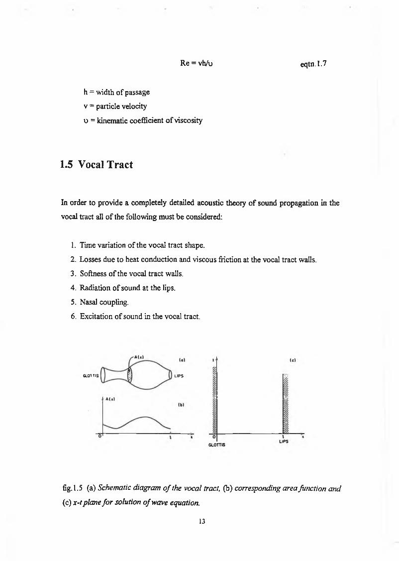
1 . 5 V o c a l T r a c t

In order to provide a completely detailed acoustic theory o f sound propagation in the

vocal tract all o f the following must be considered:

1. Time variation o f the vocal tract shape.

2. Losses due to heat conduction and viscous friction at the vocal tract walls.

3. Softness o f the vocal tract walls.

4. Radiation o f sound at the lips.

5. Nasal coupling.

6 . Excitation o f sound in the vocal tract.

fig. 1.5 (a) Schematic diagram o f the vocal tract, (b) corresponding area function and

(c) x-t plane fo r solution o f wave equation.

L IP SGL0 1 TIS

13

However, many simplifications are required in order to provide a useful numerical

physical configuration o f practical interest. The vocal tract is modelled as a tube of

non-uniform, time varying cross-section. Plane wave propagation is assumed for all

the vocal tract. Furthermore, no energy losses due to either thermal conduction or

viscosity are assumed to occur. With these assumptions, applying the laws o f

conservation of mass, momentum and energy to sound waves in the tube o f fig. 1.5,

where

p = p(x,t) is the variation of sound pressure

in the tube at position x and time t.

u = u(x,t) is the variation in volume velocity

flow at position x and time t.

p is the density o f air in the tube

c is the velocity o f sound

A = A(x,t) is the “area function” o f the tube;

i.e. the value o f cross-sectional area normal to the axis o f the

tube as a function of a distance along the tube and as a function

o f time.

Using a variety o f simplifications and approximations some straight forward solutions

are possible. Considering a constant area function for the vocal tract which is

model o f speech production. The schematic diagram in fig. 1.5 shows the simplest

frequencies below 4 kHz i.e. wavelengths that are long compared to the dimensions o f

Portnoff1 9 has shown that the following pair o f partial differential equations are

satisfied:

d pP eqtn. 1.7

ô x Ô t

Ô X

â u 1 £ ( P A ) +ô t

ô A ô t

eqtn. 1 . 8

14

approximately correct for the neutral vowel /UH/ reduces the partial differential

equation to the following form

- d p p d u - d u p d p

d x T 7 T ; ~ ~ a T eq tn 1 -9

which have the familiar travelling wave solutions

u ( x , t ) = [ u + { t - X/ c ) - U ~ ( t + x/ c ) ]

p ( x , t ) = + “ ^ ) - + 5 ^ ) ]

eqtn. 1.10

The frequency domain representation o f this model is obtained by assuming a boundary

condition at x = 0 of

U ( 0 , t ) = d ) — U G 6 J eqtn. 1.11

that is, the tube is excited by a complex exponential variation o f volume velocity o f

radian frequency © and complex amplitude, Ug(g>). Since equation 1.9 is linear , the

solution u+(t-x/c) and u'(t+x/c) must be o f the form

u * ( t - x / c ) = K * e >a u - ' X )

U ~ ( I + x/ c ) = A[ - e l Q eqtn. 1.12

Substituting these equations into eqtn. 1.10 and applying the boundary condition p(l,t)

= 0 at the lip end o f the tube and eqtn. 1 . 1 1 at the glottis end we can solve for the

unknown constants K+ and K\ The resulting sinusoidal steady state solutions are

15

/ j \ * r7 s i n [ Q ( / —x ) / c ] j r / \ i d tp ( x , t ) = j Z 0 - cl0 , ( 0 „ -c l - U g ( 0 ) e J

« ( * > o = ) ^ ‘

where

Z0= pc/A eqtn.1.14

eqtn.1.13

is by analogy to transmission line theory called the characteristic acoustic impedance of

the tube. The frequency response allows us to determine the response o f the system to

arbitrary inputs, not only sinusoids, through the use o f Fourier analysis. For more

realistic models, including the effects o f vocal tract losses and radiation at the lips, the

reader is referred to Rabiner and Schafer20.

1 . 6 A c o u s t i c A n a l y s i s o f P a t h o l o g i c a l V o i c e

Acoustic analysis as used in the vocal pathology literature and as mentioned above has

come to mean any spectrum or waveform measurement taken from the digitised speech

signal. The purpose o f the present thesis is to investigate the currently available

acoustic measures2, to test their validity and to introduce new measures. A study of

the presently available approaches has revealed that ( 1) they offer limited information

for use in clinical investigations and (2) many measurement problems arise and that the

separation o f the acoustic indices into independent measures is not a simple issue21.

More specifically, the most commonly used acoustic measures for diagnosis o f vocal

pathology are jitter, shimmer and the harmonic to noise ratio. However, several

researchers have shown that these measures are not independent and therefore may

give ambiguous information. For example, the addition o f random noise causes

increased jitter measurements and the introduction o f jitter causes a reduced harmonic

to noise ratio. The previous section was included in order to show the effect o f the

16

vocal tract on the output radiated speech waveform. The effect o f these tract

resonances have been cancelled by various strategies using inverse filtering o f a high

fidelity true phase recording o f the output airflow from the lips. Recent studies have

shown that the glottal waveform may be estimated from tape recorded speech samples

using a frequency domain parameter set22. Therefore more is being learnt about the

glottal flow and hence vibratory pattern of the vocal folds in terms o f spectral

measurements. Hanson16, Holmberg23, Karlsson24 and others have shown that many

useful acoustic parameters can be obtained from the acoustic speech waveform.

However, in order to provide spectral characterisation o f the vibratory pattern in

pathological voice types the effects o f jitter and shimmer on the speech spectrum must

firstly be removed.

These issues have been thoroughly addressed in this thesis and the foundation has been

laid for future studies that will investigate the vibratory pattern o f the vocal folds based

on spectral evaluation o f tape recorded data. Firstly, an attempt has been made to

spectrally characterise the four perturbation measures o f additive noise, random jitter,

cyclic jitter and shimmer, therefore providing a means of taking quantitative

perturbation specific measurements from the speech spectra. Secondly, novel analysis

programs have been written in order to overcome the contaminating effects o f the

perturbation measures and therefore provide a means o f assessing the vibratory

characteristics o f the vocal folds. Time domain measures have also been investigated

and the indications are that this requires further study. It is hoped that these research

efforts will complement the work o f Hanson16, Holmberg23, Karlsson24 and others in

providing more reliable acoustic indices with which to investigate both the vocal

mechanism and voice quality.

Another important issue is whether future improvement in modelling voice production

(Flannagan25, Fant22, Hirano26, Fujimura27, Titze28, Farley29) and enhanced acoustic

analysis will be able to provide differential diagnoses with respect to organic and

psychogenic disorders. This is not a simple question to answer directly, but what is

definitely true is that improved modelling and analysis o f pathological voice types will

definitely occur. One can envisage the culmination o f several research efforts

dedicated to voice, providing, not in the too distant future, a 3-D computer model o f

the larynx where many physiological parameters relevant to voice are included and

17

manipulated and the user is provided with synthesis feedback and spectral information

regarding the voicing possibilities associated with a given configuration. Images taken

from patient larynges via cinematography or ultrasound could then be matched to the

model and if after matching the synthesis sounds the same as the patient it could be

assumed that the correct model has been obtained. If the synthesis sounded different

further model alterations could be made until the synthesis matched. Having obtained

the correct match, correct alterations could be made until ‘normal’ voice was obtained.

However this is o f course beyond the scope o f this thesis and here we concern

ourselves with developing new analysis techniques that differentiate between normal

and pathological voice types.

18

1.7 Bibliography

1. Robbins, SD. A dictionary o f speech pathology and therapy. Cambridge, Mass.:

Sci-Art publishers, 1963

2. Emanuel, FW. And Sansone FE. Some spectral features o f ‘normal’ and simulated

‘rough’ vowels. Folia Phoniat. 1969; 21:401:415

3. Bielamovicz, S. et al Comparison o f voice analysis systems for perturbation

measurement. J. Speech Hear. Res. 1996; 39: 126-134

4. Titze, IR. Towards standards in acoustic analysis o f voice. NY: Raven Press J.

Voice 1994; 8 : 1-7

5. Titze, IR. Definitions and nomenclature related to voice quality, In O. Fujimura and

M. Hirano (Eds.), Vocal Fold Physiology : Voice quality control, Singular

publishing group, San Diego, 1995; pp. 335-342

6 . Deller JR. et al Discrete time processing of speech signals, New York:Macmillan,

1993, pp. 110

7. Ladefoged, P. Discussion o f phonetics : a note on some terms for phonation types,

In O. Fujimura (Ed.), Vocal fold physiology : Voice production, mechanisms and

functions, New York: Raven Press, 1988; pp.373-376

8 . Laver, J. The phonetic description o f voice quality. New York:Cambridge

University Press, 1980.

9. Imaizumi, S. Annual Bulletin RILP, University o f Tokyo, Tokyo, 19: 179-190,

1985

10. Hammarberg, B and Gauffin, J. Perceptual and acoustic characteristics o f quality

differences in pathologic voices as related to physiological aspects, In O. Fujimura

and M. Hirano (Eds.), Vocal Fold Physiology : Voice quality control, Singular

publishing group, San Diego, 1995; pp.283-303

11. Aronson, AE. Clinical voice disorders. New York: Thieme, 1990

12. Hirano, M. Clinical examination o f voice. New York: Springer-Verlag , 1981

13. Baken, RJ. Clinical measurement o f speech and voice. London: Taylor and Francis

Ltd., 1987

19

14. van den Berg, J. Myoelastic-aerodynamic theory of voice production. J. Speech

and Hearing Res. 1958; 1:3, 227-245.

15. Lieberman, P. Vocal cord motion in man. Ann. N.Y. Acad. Sci., 155:28-38, 1968

16. Hanson, HM. Glottal characteristics o f female speakers; Acoustic correlates. J.

Acoust. Soc. Am. 1997; 101:466:481

17. van den Berg, J. On the air resistance and Bernoulli effect o f the human larynx. J.

Acoust. Soc. Amer. 1957, 29:626-631

18. Stevens, KN. Airflow and turbulent noise for fricative and stop consonants , J.

Acoust. Soc. Am. 1971, 50:1180:1192

19. Portnoff, MR. and Schafer RW. Mathematical considerations in digital simulations

o f the vocal tract, J. Acoust. Soc. Am. 1973, 53:294

20. Rabiner L. and Schafer R. Digital processing o f speech signals. Englewood Cliffs,

N.J.: Prentice Hall, 1978

21. Hillenbrand, J. A methodical study of perturbation and additive noise in

synthetically generated voice signals. J. Speech Hearing Res. 1987, 30:448-461

22. Fant, G. and Lin, Q. Frequency domain interpretation and derivation of glottal flow

parameters. STL-QPSR 1988, 2-3:1-23

23.Holmberg, EB. Comparisons among aerodynamic, electroglottographic and

acoustic spectral measures o f female voice. J. Speech Hearing Res. 1995,

38:1212:1223

24. Karlsson, I. Glottal waveforms for normal female speakers. J. Phon. 1986,

14:415:419

25. Flanagan, JL.et al. Synthesis o f speech from a dynamic model o f the vocal cords

and vocal tract. Bell System Tech. J. 1975, 54:485-506

26. Hirano, M. Morphological structure o f the vocal cord as a vibrator and it’s

variations. Folia Phoniat. 1974, 26:89-94

27. Fujimura, O. Body-cover theory o f the vocal fold and it’s phonetic implications.

In K. Stephens and M. Hirano (Eds.) Vocal fold physiology. Tokyo: University of

Tokyo Press 1981, pp.271-288,

28. Titze, I. Preliminaries to the body-cover theory of pitch control. J. Voice, 1988,

1:314-319

20

29. Farley, GR. A biomechanical laryngeal model o f voice fO control and glottal width

control. J. Acoust. Soc. Amer. 1996, 100:3794-3812

21

Chapter 2

Experimental Apparatus, Technique and

Data

2 . 1 S p e e c h A n a l y s i s E n v i r o n m e n t

The equipment necessary to carry out speech analysis research is well within the budget

resources o f any university or speech therapy department1. The basic requirements are

a standard personal computer (PC) with an additional plug-in I/O module and some

means o f recording the acoustic speech waveform. This comprises a surprisingly

powerful analysis environment with dedicated digital signal processing (DSP) chips

providing real-time processing and feedback if required at moderate extra cost. The

system implemented in the present study is shown schematically in fig. 2 .1.

2.1.1 Data Acquisition

Speech samples were recorded using a standard linear dynamic microphone (SONY F-

VS3N, Tokyo, Japan) connected to a CT-W851R PIONEER double cassette deck tape

recorder (Pioneer T-W851R, Tokyo, Japan). TDK chrome tape cassettes o f 57dB

22

Mic. Stereo

»

5 S S i

■V— ---------IL - - - * il

P.C.fig. 2 .1 Schematic Diagram o f Speech Analysis System

signal to noise ratio were used with subsequent playback through a stereo amplifier

unit (Sony F I 70, Tokyo, Japan). Alternatively, direct digitisation was also possible,

with the tape deck set in record mode. The resulting continuous time signal had then

to be band limited prior to sampling in order to avoid aliasing, an unfortunate

consequence o f the well known sampling theorem2. An eight order Chebychev low

pass filter3,4 with -48 dB/octave roll off at 3.8 kHz and 2 dB ripple across the pass band

was constructed for this purpose. The filter response was examined by applying signals

in the frequency range from D.C. to 10 kHz from a Thurlby/Thandar TG220 2Mhz

Sweep/Function Generator (Huntington, Camb., England) (fig. 2.2). This bandwidth

limited analog signal could now be digitised.5 A sampling rate o f 10 kHz using pacer

trigger mode conversion was chosen from the C software driver for a 14-bit resolution,

23

variable sampling frequency, data acquisition expansion card (Integrated Measurement

Systems PCL-814, Southampton, UK) installed in an 80486DX LEO PC.

fig.2.2 Frequency response o f Chebychev low pass filte r

The resulting digitised samples were stored in 2 ’s complement (integer type) binary

form in two separate data buffers giving a total sample length o f approximately 6.5

seconds. The data was then routinely saved to disk in binary file format for subsequent

analysis.

2.1.2 Software Programming

Both Borland’s Turbo C++ (Scott’s Valley CA, USA) and Matlab (The Math Works

Inc., Natick, Mass., USA) programming environments were used for analysis. In the

case o f Turbo C++ the compiler was a DOS application operating in an Integrated

Development Environment. The project file option available with this compiler made

for efficient programming with separately compiled files being linked together at run

time. For the present application the main modules o f a project file generally consisted

o f a) the software driver for the A/D card, b) the FFT radix-4 algorithm from

Numerical Recipes in C (Cambridge University Press, Portchester, CA, USA) 6,7 and c)

24

the user written specific application program. The main user written C++ analysis

program files were used for spectrogram production purposes.

The Window’s based Matlab technical computing environment was introduced at a

later stage and greatly decreased the time necessary for coding the required analysis

and display algorithms owing to it’s high level language interface. The accompanying

Digital Signal Processing Toolbox (The Math Works Inc., Natick, Mass., USA) with

it’s specialised DSP functions was also obtained to provide the complete analysis

system. The final versions o f the principal analysis files written in Matlab are given in

appendix A.

2 . 2 R e c o r d i n g s

a) Speaker Identification Experiment

All recording were taken in a quiet room in the college using the analysis equipment as

outlined in paragraph 2.1.1. Experimental details are given in the next chapter as

appropriate, alongside the description o f the speaker identification experiment.

b) Diagnostic Investigations

The above recording procedure could not be followed in the clinical setting. Here,

recordings were made o f the participants phonating the sustained vowel a/ and uttering

the phonetically balanced sentence “Joe took father’s shoe bench out” at their

comfortable pitch and loudness level. All recordings were taken by a member o f the

research group using a Tandberg audio recorder (AT 771, Audio Tutor Educational,

Japan) prior to the participants (thirteen in all) undergoing laryngovideostroboscopic

(LVS, Endo-Stroboskop, Atmos, Germany) evaluation8 at the outpatient’s ENT clinic

in Beaumont Hospital, Dublin. The videostroboscopic evaluation was carried out by

the otolaryngologist in collaboration with the speech therapist. The LVS system

(fig.2.3) consists o f a rigid endoscope which is guided posteriorly through the patient’s

25

oropharynx until a clear image of the vocal folds is obtained. The patient is asked to

phonate the vowel a/ or i/ while under examination. Illumination is provided via strobe

pulses reflected from a laryngeal mirror attached to the end o f the endoscope.

fig.2.3 Schematic Diagram o f Laryngeal examination using

videostroboscopy

When the pulse rate ‘matches’ the pitch frequency a clear video image is obtained o f

the vocal fold vibratory pattern. Supra-laryngeal structures may also be viewed.

Hence, it provides a site specific, quantifiable assessment o f the larynx. A word of

caution is needed however, in respect to interpreting these images, especially in cases

involving vocal pathology. As the images were obtained under strobe lighting, the

apparent glottal cycle that the observer views are taken over several cycles (typically

24) o f actual vocal fold movements. Therefore, there is an inherent assumption that

the signal source is periodic which is clearly not the case with many vocal fold

pathologies. So what results in one apparent cycle may have come from several cycles

which vary widely and in many cases obtaining an image is not possible as was the case

here. Along with the results o f the stroboscopic examination, full medical details

regarding the vocal pathology were taken for each patient as well as any further

diagnostic comments at the time o f assessment. Patient details are outlined in table 2.1.

26

P A T IE N T NO . A G E SEX P A T H O L O G Y

1 39 fVocal cord nodules (bilateral)

2 70 mhoarseness

3 43 fvocal cord oedema /nodules

4 33 mvocal nodule

5 22 fleft vocal cord nodules (bilateral)

6 22 fhoarseness (on/off)

7 43 mverucous carcinoma of both folds

8 65 mHyperkeratosis and parakeratosis

9 57 fmild swollen vocal cords

10 74 mcarcinoma post-radiation right vocal cord immobile

11 23 fleft vocal cord palsy Immobile- well compensated right cord

12 54 mlaryngeal papilloma ptosis

13 57 fabductor palsy

Table 2.1 Patient listing and details. M ean age 46.3, std. dev. 20.6

The audio (and video) data from the stroboscopic evaluation was recorded using

SONY SVHS (E-180, France) cassettes. Twelve normals were subsequently recorded

under the same conditions.

27

2 . 3 A i m o f A c o u s t i c E v a l u a t i o n

From the data recorded in 2.2 a number o f investigations are possible

1) To separate the patients and normals based solely on acoustic analysis o f the

audio recording9,10.

2) To correlate the acoustic findings with assessments based on the

stroboscopic assessment11,12, the overall medical evaluation or a perceptual

evaluation13,14.

3) To assess the effects o f the endoscope on normal phonation.

This thesis reports the results o f investigation number one above. Number two could

not be attempted, unfortunately, due to lack o f viewing facilities in the case o f the LVS

recordings and no GRBAS scale rating15 or equivalent in the case o f the perceptual

evaluation. However, a simple perceptual rating scale, based on a system proposed by

Hammarberg et al was used for both the patient and normal data (Table 2.2 and 2.3) in

order to provide a more complete assessment with respect to number one above. Part

three forms the basis o f ongoing research, the results o f which will be presented

elsewhere.

NORMAL NO./

VOICE

QUALITY

1 2 3 4 5 6 7 8 9 10 i l 12

Normal (Quality) y ✓ y ✓ / y y y yBreathy ✓ ✓

Hyperfunctional ✓

Roughness /

Unstable Pitch/ y

Table 2.2 Perceptual Evaluation fo r 'Normals '. M ean age 26.5, std. dev. 3.5

28

PATIENT NO./

VOICE

QUALITY

1 2 3 4 5 6 7 8 9 10 h 12 13

Aphonic

Breathy y y ✓ y y

Hyperfunctional y y y y y ✓ y

Hypofiinctional

Fry/Creaky ✓ ✓

Roughness ✓ y y y

Gratings y y y /

Unstable pitch y y y

Voice breaks y y y y y

diplophonia y y

(a)PATIENT NO./

VOICE

QUALITY

1 2 3 4 5 6 7 8 9 10 i l 12 13

Aphonic

Breathy y y /

Hyperfunctional / y y y y y y y

Hypofiinctional y y

Fry/Creaky y y

Roughness / y y

Gratings

Unstable pitch y y y y y

Voice breaks y y y y

diplophonia y

(b)

Table 2.3 Perceptual Evaluation fo r patients a) Therapist I b) Therapist 2

29

In the case of the normal data, two o f the ‘normals’ showed deviant voice qualities, the

equivalent o f a rating o f one on a five point scale where zero represents normal and

four indicates severe dysphonia. All patient data show deviant qualities (as rated by

two speech therapists) but unfortunately the degree is not given and therefore the

perceptual ratings were used simply as a accompaniment to the acoustic findings,

rather than as the basis for correlation.

2 . 4 V o w e l S y n t h e s i s

In order to test the analysis programs for evaluation o f vocal pathology in a systematic

way vowel synthesis data files were produced. These were designed to simulate

various commonly found acoustic characterisations o f vocal pathology such as jitter

and shimmer. The discrete time system model for speech production16,17,18 shown in

fig. 2.4(a) forms the basis for this approach.

Adequate synthesis can be performed using this model to produce continuous speech

where the vocal tract parameters vary with time as appropriate. In order to introduce

the various perturbation measures certain adjustments to the model are required as

shown in fig. 2.4(b). Instead o f simply replacing the traditional exclusive OR gate

switch for voiced/unvoiced excitation with an OR gate in order to simulate conditions

o f turbulent glottal flow concurrent with normal voicing, a signal dependent random

noise component was introduced at the glottal source as shown in part (b) o f the

figure. The noise component was introduced in this manner in acknowledgment o f the

fact that for voiced fricatives, frication is correlated with the peaks o f the glottal flow.

What is the most pertinent way to represent the noise component for conditions

involving vocal pathology is uncertain and is most likely somewhat variable depending

on the specific pathology under investigation and certainly merits further study. The

vocal tract parameters are kept constant in order to produce a sustained vowel. A

randomised gain factor may also be added to the impulse train generator in order to

produce amplitude perturbation o f the glottal source. Each stage of the model is

30

examined below but we can get some idea o f the complexity o f the problem posed by

acoustic analysis o f vocal pathology through examining fig. 2.4 (b) and considering that

we are trying to reveal or separate (if possible) the source o f the abnormality

introduced at A), B), C) or D) by analysing a signal that has been convolved with the

vocal tract response and radiated at the lips. Furthermore, the model assumptions of

source/tract separability and non time-varying vocal tract parameters are only

approximately correct, even in the case o f a sustained vowel phonation.

PITCH PEHWO

iM PoiseTRAIN

GENERATOR

Gl o t t a lp u l scMODEL

GU> VO C A L TR A C T P A R A M E TE R S

Pitch Period

ImpulseTrain

B

GlottalPulse

VocalTract

Radiation

PL(n)

UG(n)

RandomNoise

D

fig.2.4 (a) Discrete time system model fo r speech production and (b)

modification o f the model fo r use in investigation o f vocal pathology

31

2.4.1 Excitation

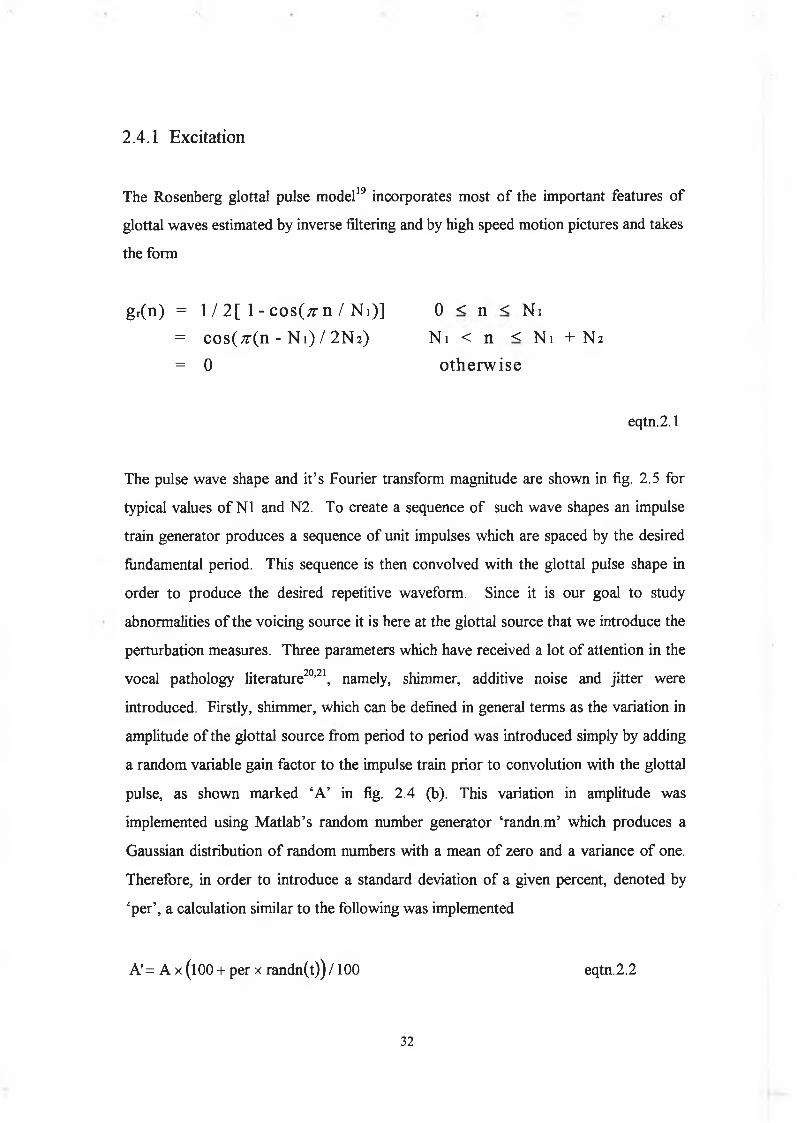
The Rosenberg glottal pulse model1 9 incorporates most o f the important features of

glottal waves estimated by inverse filtering and by high speed motion pictures and takes

the form

gr(n) = 1 / 2[ 1 - c o s (;rn / N i)] 0 < n < Ni= cos(/r(n - N i) / 2 N 2) Ni < n < Ni + N 2

= 0 otherw ise

eqtn.2 . 1

The pulse wave shape and it’s Fourier transform magnitude are shown in fig. 2.5 for

typical values o f NI and N2. To create a sequence o f such wave shapes an impulse

train generator produces a sequence of unit impulses which are spaced by the desired

fundamental period. This sequence is then convolved with the glottal pulse shape in

order to produce the desired repetitive waveform. Since it is our goal to study

abnormalities o f the voicing source it is here at the glottal source that we introduce the

perturbation measures. Three parameters which have received a lot o f attention in the

vocal pathology literature20’21, namely, shimmer, additive noise and jitter were

introduced. Firstly, shimmer, which can be defined in general terms as the variation in

amplitude of the glottal source from period to period was introduced simply by adding

a random variable gain factor to the impulse train prior to convolution with the glottal

pulse, as shown marked ‘A ’ in fig. 2.4 (b). This variation in amplitude was

implemented using Matlab’s random number generator ‘randn.m’ which produces a

Gaussian distribution o f random numbers with a mean o f zero and a variance of one.

Therefore, in order to introduce a standard deviation o f a given percent, denoted by

‘per’, a calculation similar to the following was implemented

A'= A x (lOO + per x randn(t)) /100 eqtn.2.2

32

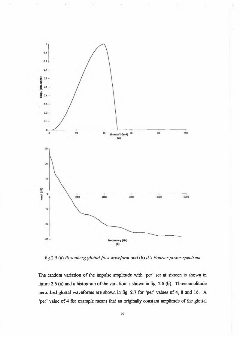
(a)

fig. 2.5 (a) Rosenberg glottal flow waveform and (b) it's Fourier power spectrum

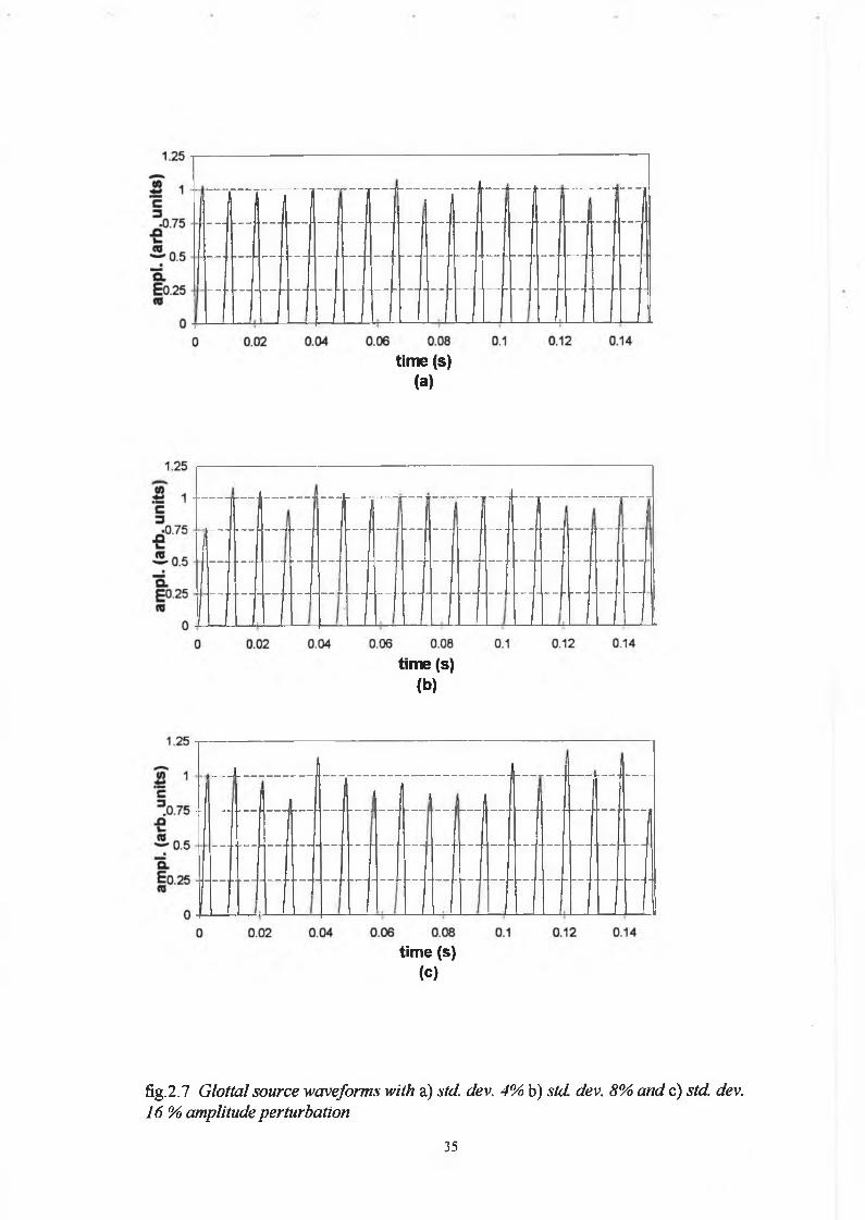
The random variation o f the impulse amplitude with ‘per’ set at sixteen is shown in

figure 2.6 (a) and a histogram o f the variation is shown in fig. 2.6 (b). Three amplitude

perturbed glottal waveforms are shown in fig. 2.7 for ‘per’ values o f 4, 8 and 16. A

‘per’ value o f 4 for example means that an originally constant amplitude o f the glottal

33

uipL

(a

rti,

unita

)source, ‘A’, now has a Gaussian distributed amplitude with a standard deviation equal

to 4% of the original amplitude.

I m p u l a a T r a i n A m p l i t u d e N u m b e r <*)

(b)

fig.2.6(a) Random variation o f amplitude o f impulse train and (b) histogram o f

the variation

34

time (s) (a)

time (s) (b)

time (s) (c)

fig.2.7 Glottal source waveforms with a) std. dev. 4% b) std. dev. 8% and c) std. dev. 16 % amplitude perturbation

35

The introduction of random noise and random pitch perturbation followed a similar

strategy. Random additive noise was introduced by multiplication o f the glottal pulse

waveform by a random noise generator arranged to give signal dependent additive

noise o f a user specified variance, denoted ‘per’ in the Matlab program ‘synadnoq.m’.

The noise was added according to the following equation

gr' = gr x ( l 0 0 + per x randn(n) ) / 1 0 0 eqtn.2.3

time (s*10e-4) (a)

(b)

time (s*10e-4)(c)

fig.2.8 Signal dependent, random, additive, Gaussian noise a) std. dev. 4 % b) std.

dev. 8 % and c) std. dev. 16%

36

As a result o f this, greater noise occurs at peak flow but the signal to noise ratio

remains constant at all points along the waveform during the open phase. Three

additive noise levels o f standard deviation 4, 8 and 16 percent are shown for the 110

Hz file in figure 2.8. Applying the noise in the above manner insures that the closed

phase remains unaffected by the noise.

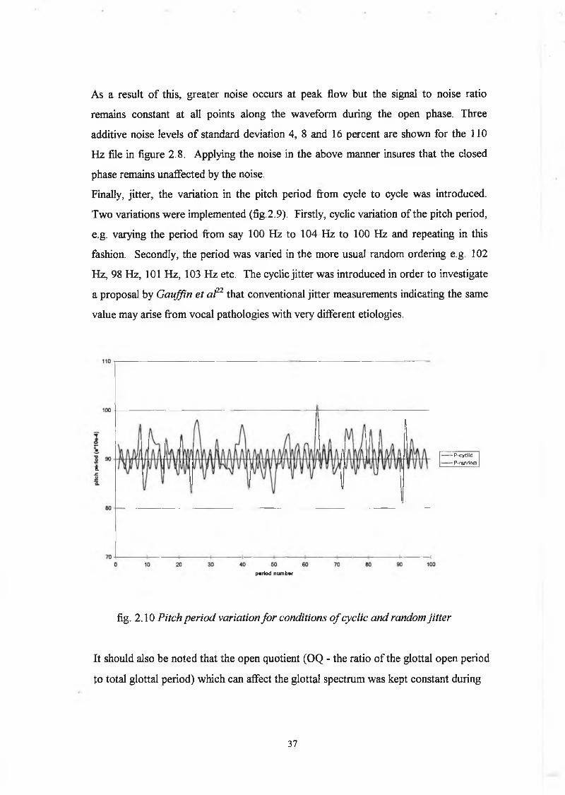
Finally, jitter, the variation in the pitch period from cycle to cycle was introduced.

Two variations were implemented (fig.2.9). Firstly, cyclic variation of the pitch period,

e.g. varying the period from say 100 Hz to 104 Hz to 100 Hz and repeating in this

fashion. Secondly, the period was varied in the more usual random ordering e.g. 102

Hz, 98 Hz, 101 Hz, 103 Hz etc. The cyclic jitter was introduced in order to investigate

a proposal by G auffin et al22 that conventional jitter measurements indicating the same

value may arise from vocal pathologies with very different etiologies.

■c 2.

- P-cyclic

-P -random

period number

fig. 2.10 Pitch period variation fo r conditions o f cyclic and random jitte r

It should also be noted that the open quotient (OQ - the ratio o f the glottal open period

to total glottal period) which can affect the glottal spectrum was kept constant during

37

all the above perturbation variations, as opposed to simply truncating the period as in

often done in multi-pulse resynthesis when introducing pitch perturbation. We avoid

this approach as we want to vary fO as an independent parameter o f change, with a

view to future studies that would focus on events that occur within the glottal cycle.

This corresponds to the source o f variation introduced at B in the schematic diagram of

fig. 2.4 (b). Ananthapadmanabha2 3 has shown that the open quotient is inversely

proportional to the harmonic ratio, where the harmonic ratio (HR) is defined as the

ratio o f the amplitude o f the second to the first harmonic. Therefore, had we simply

truncated the closed phase we would have changed the spectral content o f the signal as

a result o f a change in open quotient as opposed to simply an fO increase.

2.3.2 Vocal Tract Model

These glottal pulses are now used to excite the vocal tract, the transmission properties

of which in our digital model are based on the behaviour o f a set o f concatenated

lossless acoustic tubes as shown in fig. 2 . 1 1 .

I

■A*

1

A, A * A i A a A

**-Ax — —

F a T-Ax

-Ax

•Ax •Ax -*»

GLOTTIS LIPS

fig. 2.11 Concatenated Lossless Tube M odel

Portnoff2 4 has shown that sound waves in a tube satisfy the pressure/volume velocity

relationship

38

Pk(x,t) = ^ Ax

Uk'(t-----) + Uk~(t+—)C CX X

X XUk(x, t) = Uk(t - — ) - Uk(t + — )

c c

eqtn.2.4

pt = pressure at k* tube

ut= volume velocity at k* tube

p = density o f air

where x is the distance measured from the left hand end o f the k* tube (0 <x<lt) and

ut+ 0 and Uk- 0 are positive going and negative going travelling waves in the k* tube.

Lossless and plane wave propagation assumptions, along with boundary conditions at

the tube junctions obtained by applying the physical principle that pressure and volume

velocity must be continuous in both time and space everywhere in the system, give rise

to relatively straight forward solutions o f the resulting equations, known as the

Kelly/Lochbaum equations. 2 5 These equations can be usefully depicted using signal

flow graph conventions1 6 where x = Ax/c is the one way propagation o f the sections

(fig.2.12a). This representation (or equivalently from fig.2.11) implies that the lossless

tube models have properties in common with digital filters. An equivalent discrete time

lattice filter is shown in part b) o f the figure.

(4*) (i ••,)

(a)

•'U’ (tM.IuetnTI

IIuJflT)

fig.2.12 a) Signal flaw graph fo r lossless tube model o f the vocal tract; b) equivalent

discrete time system

For a discrete time vocal tract model consisting o f a concatenation o f N lossless tubes

of equal length the system function is

39

For a discrete time vocal tract model consisting o f a concatenation o f N lossless tubes

o f equal length the system function is

V ( z ) = f i O + rk ) z ' N 12eqtn.2.5k -1

D ( z )

w here the denom inator D ( z ) is obta ined from the p o lyn om ia l recursion

D o(z) = 1

D k ( z ) = Dk - i ( z ) + r k z ‘kDk k = 1 , 2 , . . . ,ND ( z ) = D n ( z )

where the rt’s are the reflection coefficients at the tube junctions,

rk = Ak + i - Ak

A_k + 1 + Ak

and it is assumed that there are no losses at the glottis and that all losses are

introduced at the lip end through the reflection coefficient

The system function can also be written in the form o f a direct-form difference

equation as

TN — TL — A n t I - A k

A N + I + A N

1 - a kz‘kN

G

eqtn,2.6

40

Hence, given a set o f area data the system function can be obtained. Fant2 6 has

supplied such data obtained from x-ray images o f the phonation of the Russian vowel

AA (Table 2.4).

SECTION 1 2 3 4 5 6 7 8 9 1 0

vowel AA 1 . 6 2 . 6 0.65 1 . 6 2 . 6 4 6 . 8 7 5

Table 2.4 Vocal tract area data for Russian vowel AA (cm2)

Radiation at the lips is simply modelled by the first order difference equation R(z) = (1-

z‘l) to supply the final ingredient in our model. The waveform for the vowel AA at 110

Hz is shown in fig.2.13.

time (s*10e-4)

fig.2.13 Synthesis vowel AA - G lottal pulse o f fig .2 .5 filtered using the digital model

o f the vocal tract transfer function.

41

2.4.2 Vowel Data

The actual implementation of the above synthesis model was performed using a user

written program (synthOQ.m) with calls to the signal exercises library for the AtoV

function and Matlab’s filter function. The program listings are given in appendix A.

Tables 2.5 and 2.6 give a complete list o f the data files produced to provide a means of

testing and calibrating the subsequent analysis programs.

Table 2.5 List o f synthesis data fo r 110 Hz signal

RANDOM JITTER (STD DEV.)

PERIODIC (OR CYCLIC) JITTER (%)

ADDITIVE NOISE (STD DEV.)

SHIMMER (STD DEV.)

1 1 1 12 2 2 23 3 4 44 4 8 85 5 16 166 6 32 32

T able 2.5 L ist o f synthesis data fo r 220 H z signal

RANDOM JITTER (STD DEV.)

PERIODIC (OR CYCLIC) JITTER (%)

ADDITIVE NOISE (STD DEV.)

SHIMMER (STD DEV.)

1 1 4 13 3 8 45 5 16 16

Further files were also created for three levels o f noise for signals beginning at 80 Hz

and increasing in six, approximately equi-spaced steps of 60 Hz up to 350 Hz.

42

2.5 Bibliography

1. Curtis, J.F. An introduction to microcomputers in speech, language and hearing,

Little Brown and Co., 1987

2. Oppenheim, A.V. and Schafer, R.W. Discrete-time signal processing. Englewood

Cliffs, N.J.: Prentice Hall, 1989

3. Lancaster, D. “Low-pass and high-pass filter responses”, in The active filter

cookbook. Indianapolis: Howard W. Sams & Co., 1987

4. Horowitz, P. and Hill, W. The Art o f Electronics. Cambridge Mass..Cambridge

University Press, 1986

5. Oppenheim, A.V. Applications of digital signal processing. Englewood Cliffs, N.J.:

Prentice Hall, 1978

6 . Press, W.H. et al. Numerical Recipes in C. Cambridge, USA: Cambridge University

Press, 1992

7. Sorensen, H. V. et al. Real valued fast Fourier transform algorithms. IEEE Trans, on

Acoustics, Speech and Signal Processing 1987; VOL. ASSP.35. NO. 6

8 . Koike, Y. and Imaizumi, S. Objective Evaluation of Laryngostroboscopic Findings.

In O. Fujimura (Ed.) Part VII Vocal fold physiology, Vol 2. NY:Raven Press, 1988

9. Valencia-Naranjo, N. Diagnostic voice disorders, Current Opinion in

Otolaryngology and Head and Neck Surgery, 1995 3:164-168

10. Fex, B. et al. Acoustic Analysis of Functional Dysphonia: Before and After Voice

Therapy (Accent Method). J. Voice 8:163-187

11. Suiter, A. et al. Standardised laryngeal videostroboscopic rating: Differences

between untrained and trained male and female subjects, and effects o f varying

sound intensity, fundamental frequency, and age” J. Voice 10:2:175-189

12. Woo, P. et al. “Aerodynamic and stroboscopic findings before and after

microlaryngeal phonosurgery. J. Voice 8:2:186-194

13. Hammarberg, B. and Gauffin, G. Perceptual and acoustic characteristics o f quality

differences in pathological voices as related to physiological aspects. In O. Fujimura

and M. Hirano (Eds.), Chapterl7 Vocal Fold Physiology: Voice Quality Control

San Diego: Singular Publ. Group, 1995

43

14. Lee, C.K. and Childers, D.G. Some acoustical, perceptual and physiological

aspects o f vocal quality”, In J. Gauffin and B. Hammerberg (Eds.), Vocal fold

physiology: acoustic, perceptual and physiological aspects o f voice mechanisms.

San Diego: Singular Publishing, 1991

15. Imaizumi, S. Acoustic measurement o f pathological voice qualities for medical

purposes, ICASSP, Tokyo, IEEE, 1986

16. Rabiner, L. and Schafer, R. Digitial processing o f speech signals, Englewood Cliffs,

N.J.: Prentice Hall, 1978

17. Deller, J. Proakis J. and Hansen, J. Discrete time processing o f speech signals,

NY: Macmillan, 1989

18. Burrus, C. et al. Computer-based exercises for signal processing using Matlab,

Englewood Cliffs, NJ: Prentice Hall, 1994.

19. Rosenberg, A. Effect o f glottal pulse shape on the quality o f natural vowels. J.

Acoust. Soc. Amer. 1971, 49:583-590

20. Hillenbrand, J. “A Methotological Study o f Perturbation and Additive Noise in

Synthetically Generated Voice Signals”, J. Speech Hear. Res., 30:448-461, 1987

21. Askenfelt, A. and Hammerberg, B. Speech waveform perturbation analysis: A

perceptual-acoustic comparison o f seven measures, J. Speech Hearing Res. 1986,

29:50-64

22. Gauffin, J. et al, Irregularities in the voice: A perceptual experiment using synthetic

voices with subharmonics in P. Davis and N. Fletcher (Eds.), Vocal fold physiology :

controlling complexity and chaos, San Diego: Singular Publishing, 1996

23. Ananthapadmanabha, TV. Spectral parameters o f a voice source pulse J. Acoust.

Soc. Am. 1991, 90:2345

24. Portnoff, MR. and Schafer RW. Mathematical considerations in digital simulations

of the vocal tract, J. Acoust. Soc. Am. 1973, 53:294

25. Wu, H. et al. Vocal tract simulation : Implementation o f continuous variations o f

the length in a Kelly-Lochbaum model, effects o f area function spatial sampling”

IEEE, 1987

26. Fant, G. Acoustic theory o f speech production. Mouton, The Hague, 1970.

44

Chapter 3

Investigation into Speaker Identification Using

Digital Speech Spectrograms

3 . 1 I n t r o d u c t i o n

The advance o f modern telecommunications in major industrialised nations has been

paralleled by an increase in the use o f human speech as an instrument in committing

crimes. The would be assailant has taken advantage o f the fact that the use o f the

telephone provides a means o f maintaining anonymity whilst committing a variety of

offences such as kidnappings, terrorist attacks, obscene phone calls and hoax bomb

threats.

Where live recordings exist o f an actual crime an expert witness is called upon to

decide whether (based upon scientific principles) the recorded voice is the same or

different from that o f the suspect or a list o f suspects. Forensic speaker identification

has presented many difficulties and much controversy has surrounded it’s use due the

serious nature o f the implications o f a false identification. In order to appreciate some

o f the difficulties involved in forensic speaker identification, a discussion is given of the

problem in the context o f the broader field o f speaker recognition1.

45

Speaker recognition is a generic term which refers to any task which discriminates

people based upon their speech characteristics. The potential applications o f speaker

recognition have increased with developments in telecommunications and automatic

information processing. Technological research has not been slow in developing such

applications, providing a number o f solid state devices for access control to high

security installations such as military facilities, nuclear power stations and research

laboratories. More recently, automatic telephone transaction control (e.g. telephone

banking) and tele-monitoring o f individuals on probation have been introduced with

considerable success. The basis for each of these recognition strategies is generally the

same. A person identifies himself/herself as a ‘customer’ by entering a personal code

number and is then required to pronounce a test phrase taken from a limited

combination o f words. Following some sort o f acoustic analysis, usually involving the

use o f the Long Term Averaged Spectrum, a feature vector (i.e. a vector whose

elements consist o f acoustic parameters that have been shown to carry speaker

identifying features) is derived from the test signal and matched to vectors gained from

earlier access claims of the person in question. A similarity index is then calculated and

recognition is affirmed if a certain threshold is exceeded : if not the procedure is

repeated or the person is regarded as an impostor. Typical error rates for such systems

are less than one per cent for both false rejection and false identification so can we

apply this technology to the forensic case ?

There are several factors which separate the above, so-called speaker verification task

from the more difficult task o f speaker identification, so, at present the answer is in the

negative. Firstly, the verification task involves a co-operative speaker whereas in the

forensic situation, one reason for oral communication is to conceal identity.2,3

Secondly, there are no pre-selected phrases or vowels which are known to contain

highly speaker-specific information in the forensic case. Thirdly, the vast majority of

forensic cases involve telephone transmitted speech4 where there exist several

possibilities for degradation along the transmission path and the signal is bandlimited

between 300-3400 Hz. Finally, the verification task typically involves close set

comparisons (i.e. the unknown speaker is contained within the test set), whereas in the

forensic situation the set o f potential speakers is open. So, under forensic investigation

conditions the use o f automatic methods has not seriously been considered.

46

Three further approaches to the problem have been developed however, and are

currently in use. The first is speaker identification as performed by a phonetician or

speech scientist through auditory recognition, the second is based on a semi-automatic

computer analysis approach and the third is based upon the visual comparison o f

speech spectrograms which will now be described in some detail.

3.2 The Speech Spectrogram

The speech spectrograph is a device for displaying how the acoustic patterns of speech

vary with time. It was developed by Koenig, Dunn and Lacey12 during the forties as

part o f the war effort in the US. A rich source o f information on speech spectrograms

is a book by Potter, Kopp and Green, entitled Visible Speech.13 The spectrograph is

used extensively in speech research today, providing useful information in areas such as

acoustic phonetics and speech pathology. A spectrogram for the phrase “You and I

have to go today” is shown in fig.3.1 with time plotted on the horizontal axis,

frequency on the vertical and the speech energy is plotted as a grey scale.

fig.3.1 Spectrogram o f the sentence "You and I have to go today

47

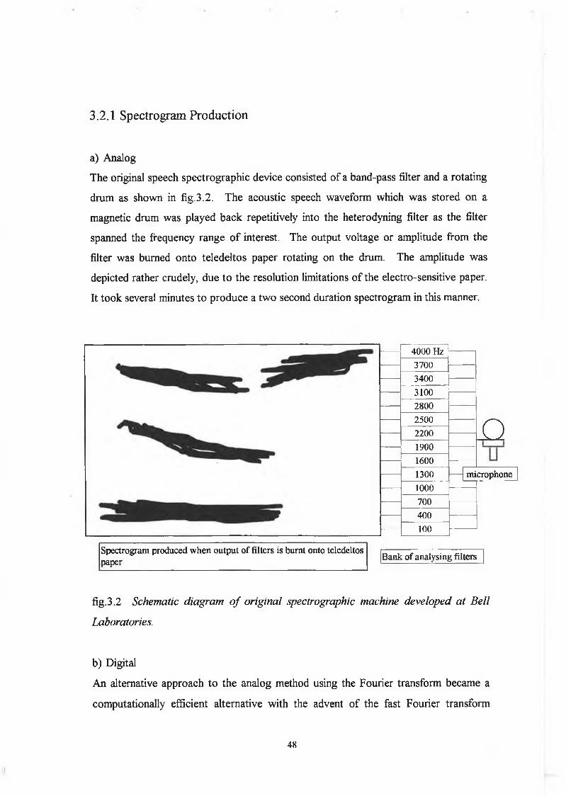
3.2.1 Spectrogram Production

a) Analog

The original speech spectrographic device consisted of a band-pass filter and a rotating

drum as shown in fig.3.2. The acoustic speech waveform which was stored on a

magnetic drum was played back repetitively into the heterodyning filter as the filter

spanned the frequency range o f interest. The output voltage or amplitude from the

filter was burned onto teledeltos paper rotating on the drum. The amplitude was

depicted rather crudely, due to the resolution limitations o f the electro-sensitive paper.

It took several minutes to produce a two second duration spectrogram in this manner.

40 0 0 H z

3700

3400

3100

2800

2500

22001900

1600

1300

1000700

400

100

Spectrogram produced when output of filters is burnt onto teledeltos paper

o

microphone

Bank of analysing filters

fig.3.2 Schematic diagram o f original spectrographic machine developed a t B ell

Laboratories.

b) Digital

An alternative approach to the analog method using the Fourier transform became a

computationally efficient alternative with the advent of the fast Fourier transform

48

(FFT) algorithm. Oppenheim7 and Melmerstein8 in 1970, were the first to suggest and

implement such a digitally based spectrographic system. As technology developed,

several improvements’ were made to these original digital speech spectrograms and

with the development o f faster processors and dedicated DSP chips the real time voice

spectrogram became a reality9. A brief review o f the spectral analysis o f speech

production serves to illustrate the motivation behind the digital spectrogram.

c) Spectral Analysis o f Speech

The process o f speech production can be modelled as a linear system with either a

quasi-periodic (voiced) excitation or a random noise (unvoiced) source as input. The

system function is the response o f the vocal tract to this input. For the production o f a

given phoneme e.g. a vowel sound, the vocal tract can be considered to remain

stationary, giving rise to a given resonant condition. The system function can then be

viewed in terms o f the impulse response or the frequency response o f the vocal tract to

this quasi-periodic input (fig. 3.3).

fig.3.3 Source/filter m odel o f speech production illustrating system characterisation

via the impulse (s(t)=v(t)*e(t)) (* denotes convolution) and frequency response

(S(co)=E(co)xV(co)), where s(t) is the output waveform, eft) the excitation source and

v(t) the vocal tract filtering. Capital letters denote Fourier transform o f time domain

counterparts.

49

The input corresponds to the glottal waveform or the volume velocity at the vocal

cords and the output corresponds to the volume velocity at the lips. If, for example,

the vowel produced was the vowel i\J as in bee, a typical set of values for the first three

resonances o f the vocal cavity are 270, 2290 and 3010 Hz. Since the glottal waveform

is periodic it’s spectrum consists o f a discrete set of harmonic frequencies. On passing

through the vocal tract these frequency components are modified (i.e. multiplied) by

the vocal tract response, providing the output spectrum. During the production of

fricative sounds such as /s/, the excitation consists o f a noise-like waveform produced

as the egressive airflow is constricted between the tongue and the teeth (labio-dental)

causing turbulent flow. Therefore, for fricative sounds, the output is noise-like and has

no line spectrum.

In ongoing speech, the vocal tract changes shape relatively slowly due to physiological

constraints on the articulators. Therefore, speech can be modelled as a linear system as

in fig.3.3 but now the filter function is seen to vary relatively slowly over time with the

resonance conditions o f the vocal tract remaining stationaiy over a period of 30 to 40

ms. It is appropriate, therefore, to view the speech waveform using a short time

spectral analysis. A short time window (~5ms) exhibits the resonance peaks o f the

system function along with the pitch period o f excitation. A longer window (~25ms)

reveals the harmonic frequency components in voiced speech as well as the spectral

envelope. The trade off is that it cannot follow rapid changes as accurately. Figure 3.4

shows the case for both the narrowband and wideband analysis, both o f which are

commonly used in speech analysis. In practice we have seen very briefly how this

analysis can be achieved via the sound spectrograph. Now, we take a look at an

alternative approach (which we will show to be equivalent) using the Fourier

transform.

d) Time Dependent Fourier Analysis10

The motivation for a short-time spectral representation which reflects the time varying

properties o f the speech waveform leads us to define the time dependent Fourier

transform

50

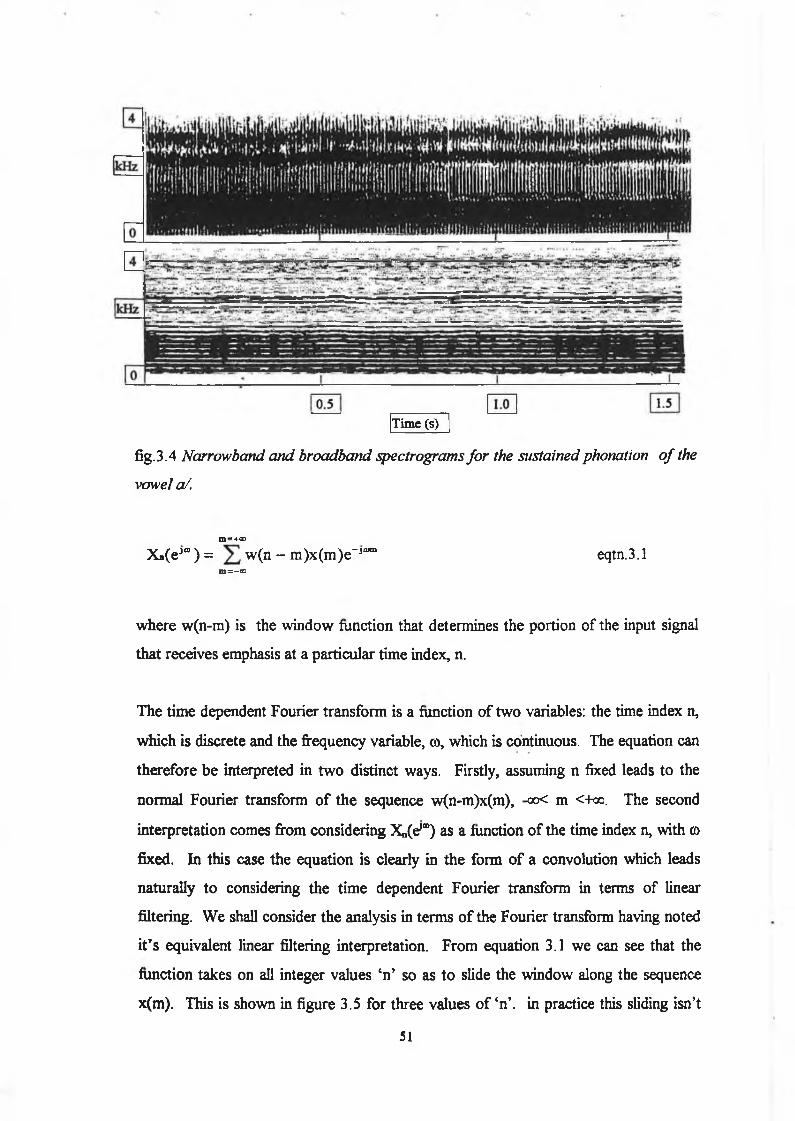
Time (s)

fig. 3 .4 Narrowband and broadband spectrograms fo r the sustained phonation o f the

\>owel a/.

m=4-c©X«(eJ® ) = w (n “ m )x(m )e”jam eqtn.3.1

m=—®

where w(n-m) is the window function that determines the portion of the input signal

that receives emphasis at a particular time index, n.

The time dependent Fourier transform is a function o f two variables: the time index n,

which is discrete and the frequency variable, ©, which is continuous. The equation can

therefore be interpreted in two distinct ways. Firstly, assuming n fixed leads to the

normal Fourier transform o f the sequence w(n-m)x(m), -oo< m <+oo. The second

interpretation comes from considering X„(e*“) as a function o f the time index n, with a

fixed. In this case the equation is clearly in the form o f a convolution which leads

naturally to considering the time dependent Fourier transform in terms of linear

filtering. We shall consider the analysis in terms o f the Fourier transform having noted

it’s equivalent linear filtering interpretation. From equation 3.1 we can see that the

function takes on all integer values ‘n’ so as to slide the window along the sequence

x(m). This is shown in figure 3.5 for three values o f ‘n’. in practice this sliding isn’t

51

necessary as we have seen that the speech signal remains essentially stationary for time

durations on the order of ten milliseconds. A computationally more efficient approach

is to ‘hop’ the window along the sequence. This can be considered as a sampling of

the equivalent linear filtering implementation.

fig.3.5 Sliding of window function along the speech sample. Three values of ‘n ’

shown.

The window has another important role besides simply selecting the segment for

analysis. The rectangular window which Fourier transforms to

<oNW (< » )= e x p (+ y — )

sinN

(O

sin1

2 “

eqtn.3.2

where N is the total sample length.

It has the narrowest main lobe but has the highest side lobes o f any o f the commonly

used windows. The result o f windowing on the spectral estimates can be explained by

viewing the time dependent Fourier transform (equation 3.1) in terms o f the Fourier

transform o f a product. As illustrated in the following equation, for fixed ‘n’, this is

equivalent to the convolution o f the two individual transforms.

1 nXn(ej" ) = — J fV(ej6)eJ0nX(e(a>+0))d0 eqtn.3.

2 1 * _ n

W(lOO-ml W( 200-m l

52

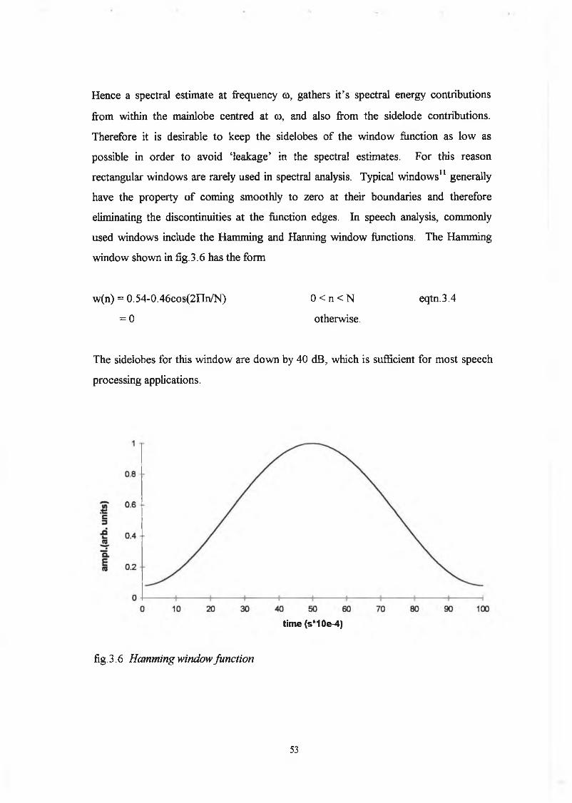
Hence a spectral estimate at frequency a , gathers it’s spectral energy contributions

from within the mainlobe centred at a>, and also from the sidelode contributions.

Therefore it is desirable to keep the sidelobes o f the window function as low as

possible in order to avoid ‘leakage’ in the spectral estimates. For this reason

rectangular windows are rarely used in spectral analysis. Typical windows11 generally

have the property o f coming smoothly to zero at their boundaries and therefore

eliminating the discontinuities at the function edges. In speech analysis, commonly

used windows include the Hamming and Hanning window functions. The Hamming

window shown in fig.3 .6 has the form

w(n) = 0.54-0.46cos(2IIn/N) 0 < n < N eqtn.3.4

= 0 otherwise.

The sidelobes for this window are down by 40 dB, which is sufficient for most speech

processing applications.

time (s*10e-4)

fig. 3.6 Hamming window function

53

3.2.2 Implementation

The actual programming o f the speech spectrogram was carried out in a Turbo C++

(Borland, Scotts Valley CA, USA) project file environment on a LEO 486DX PC. The

complete time record is broken up into segments in order to calculate the short time

Fourier transform providing a spectral cross section for each segment. Overlap

segmentation is used in order to obtain more consistent spectral estimates. The

number of points (N) required for each spectral cross section is greater in the

narrowband case but since the time resolution is worse than in the wideband case the

number o f cross sections (M) to be computed is less. M was chosen to be a fixed

percentage o f N (seventy-five per cent overlap). Since the computation o f the FFT is

proportional to Nlog2N, the analysis time for an utterance is essentially the same for

both narrowband and wideband analyses. For a 6.5 second spectrogram the analysis

time including display was approximately 30 seconds. On a Pentium PC this becomes

real time. Hardcopy was attained using a Pizzaz++ screen dump routine (Application

Techniques Inc., Pepperell, MA, USA) downloading to an inkjet printer (HP550C,

Singapore). The input speech was low passed filtered at 3.8 kHz, digitised at 10 kHz

and pre-emphasised using a first order difference equation in order to compensate for

the -12 dB/octave falloff in amplitude of the source harmonics. The time window

w(n), chosen to be a Hamming window (eqtn.3.4) was then applied. Many

combinations of window length and overlap lengths were investigated in order to

obtain the optimum display for both the narrowband and wideband spectrograms. For

the narrowband analysis the window length was chosen to be 256 giving a 6 dB filter

bandwidth o f 70 Hz. In the wideband case the length was chosen to be 75, giving 6

dB filter bandwidths o f 240 Hz. The FFT algorithm used was Numerical Recipes in C

radix-4 algorithm, four.c, incorporated into the TC++ project file. The subsequent dB

power spectrum amplitudes obtained were coded with a sixteen bit grey scale and the

spectra were plotted (using TC++ graphics functions) with respect to time in order to

produce the spectrogram display. Contour spectrograms were also produced using

fine temporal hopping o f 1 ms. It should be noted that the 6 dB bandwidths determine

the frequency resolution o f the FFT as point out by Harris11 and not the classical

54

resolution criterion of 3 dB (or half power) as stated by Morris9. This is due to the fact

that an FFT estimate is derived from the coherent addition o f spectral components

weighted through the window function. Also, the square root operation mentioned by

Morris is not necessary as all that is required for the spectrogram display is the power,

or rather the dB power spectrum.

All the literature pertaining to speaker identification based on spectrographic evidence

refers to spectrograms that have been produced via the original analog device.

However, in recent years the digital spectrogram which is commercially available in

many forms has superseded the analog device. Although, it is clear that good quality

spectrograms are available via the FFT approach, it is pertinent to compare the speaker

identification ability based on visual comparison o f these spectrograms, which have

been produced using a completely different methodology and displayed via an entirely

different hardware arrangement, with the original analog based spectrograms. An

experiment (not previously reported in the literature) was set out in order to investigate

this proposition but first we will take a brief glimpse at some of the extensive literature

regarding the controversy surrounding the use o f the original speech spectrogram for

speaker identification.

3 . 3 S p e a k e r I d e n t i f i c a t i o n B a s e d o n V i s u a l I n s p e c t i o n o f

S p e c t r o g r a m s

The dispute over the use o f spectrograms for forensic speaker identification is well

illustrated by the exchange between Koenig and Shipp et al and subsequently clarified

by Nakasone et al, which took the form o f letters to the editor o f The Journal o f the

Acoustical Society o f America. The initial letter by Koenig12 (June 1986) highlights the

main findings o f the 1979 National Research Council13 report on the reliability o f

spectrographic speaker identification under forensic conditions which were, in part:

(1) Estimates are available only for a few situations and they “do not constitute a

generally adequate basis for a judicial or legislative body to use in making judgments

55

concerning the reliability and acceptability o f aural-visual voice identification in

forensic applications” .

(2) Examiners should use all available knowledge and techniques that could improve

the voice identification method.

(3) Spectrographic voice identification assumes that intra-speaker variability

(differences in the same utterance repeated by the same speaker) is discernible from

inter-speaker variability (differences in the same utterances by different speakers):

however, that “assumption is not adequately supported by scientific theory and data.”

Viewpoints on actual error rates are presently based on “various professional

judgments and fragmentary experimental results rather than from objective data

representative of results in forensic applications”.

In order to supply such data Koenig then outlines the work undertaken by the FBI in

providing investigative support in over 2000 cases of voice identification over a period

o f fifteen years up until October, 1985. The error rates obtained for these

investigations were 0.53 % false elimination and 0.31 % false identification. The Shipp

et al reply14 (April 1987) complains about examiner training, lack o f detailed

information on the methods used and results of investigation which were considered

correct or incorrect based on whether a conviction was obtained or not (and

presumably, in the light o f other evidence relevant to the case). These objections were

then countered by Koenig et al15 who cites other literature for comparison practices.

Further clarification on the above exchanges is provided by Melvin et al16 in support of

the spectrographic method, stating that the scientific community is divided on, rather

than opposed to using the technique and they refer to Tosi’s list o f over seventy

scientists in support o f the method if practiced by trained examiners who follow the

International Association for Identification norms.

Much of the conflict regarding the use o f the spectrographic method can be attributed

to the initial paper by Kersta17, which appeared in Nature (December, 1962), in which

he introduced the method, likening the technique to fingerprinting and coining the

word ‘voiceprint’. Subsequently, Kersta became convinced of the infallibility o f the

technique which he felt was robust with regard to aging, removal of adenoids etc.. We

simply take note o f the experiment type and error rates he reported by examinations

56

carried out by high school students with one week’s training. For a group o f nine

talkers, using isolated cue words, the error rates ranged from 0 to 3 %. This

provocative paper resulted in, among other comments, calls for more extensive

research into the method and identification trials more relevant to forensic situations.

A two year experiment on voice identification was undertaken by Tosi et al in order to

test Kersta’s claims and also to introduce models relevant to the forensic task. The

reader is referred to Experiment on Voice Identification19 for the details o f the report

and again we simply state the results. The experiment confirmed Kersta’s experimental

data for closed trials o f identification and gave error rates o f 2 per cent false

identification and 5 per cent false elimination for the forensic tasks. From this bellicose

background on speaker id via the spectrographic method we simply note the error rates

and experimental conditions and techniques reported by Kersta and Tosi in order to

compare the error rates obtained using digital spectrograms.

3.4 Experim ent on Speaker Identification using Digital

Spectrogram s

Test Format:

The test format followed that o f Kersta and later copied and extended by Tosi. This

consisted o f sorting and matching experiments in closed trials o f identification on

samples recorded contemporaneously. Each speaker was asked to utter the following

words four times each - ‘it’, ‘is’, ‘on’, ‘the’, ‘you’, ‘and’, T , ‘to’, ‘me’, ‘a’, also,

he/she repeated the following sentences three times each -

‘It is on the table’

‘You and I have to go today’

‘He gave me a card’

‘He told me to put the kettle on.’

‘And I told you a few minutes ago.’

57

Forty subjects (20 male, 20 female) who were free from any form of speech pathology

supplied the above speech samples. All subjects were Irish Pre-Medical students in the

age range o f 17 to 33 years ( average = 19.5, std. dev. = 3.5 years). The speakers were

divided into four categories; 1) Male, Dublin accent, 2) Male, non-Dublin accent, 3)

Female, Dublin accent and 4) Female, non-Dublin accent.

Digital spectrograms were produced for all the above utterences. Closed set, single

utterance tests were constructed by randomly selecting six speakers from the same

speaker category. Four spectrograms per isolated word existed for each speaker. Two

spectrograms were selected as “known speaker” for each speaker for all ten words,

which left two samples per speaker to be sorted for each word as shown in fig.3.7.

The sentence procedure involved a matching experiment as opposed to the sorting

experiment for the isolated utterances. In this case two references were taken for each

speaker and the third sample, which had been chosen at random by the experimental

coordinator, was required to be matched to one of these six (fig. 3.8).

All of the comparison tests were carried out by six examiners in the age range 22 - 31

years (average = 25.2 yrs, std. dev. = 4 .5 yrs). All examiners were either academic

staff or post-graduate research students from the RCSI Dept, o f Chemistry and

Physics. The examiners were required to make a definite decision based solely on the

visual inspection o f the spectrograms. Since none of the examiners had any prior

experience with matching spectrograms, the category o f Female-Dublin-Accent was set

aside to act as a preliminary “training” set. After completing each experiment from this

training set, the experimental coordinator would tell the examiner how many incorrect

matches had been made, would identify which matches were incorrect and point out

any spectrographic features from these that might have aided in a correct identification.

Once the training set had been completed the experimental coordinator did not give any

further retrospective assistance to the examiners but did tell them their number of

incorrect matches.

58

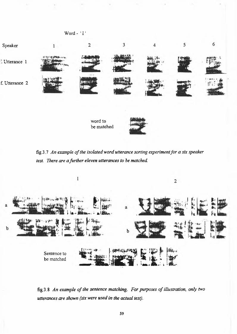
W ord - ' I '

Speaker

Utterance 1

f. Utterance 2

M ls « f r ' *>■ > : w

word to be matched

fig. 3.7 An example o f the isolated word utterance sorting experiment fo r a six speaker

test. There are a further eleven utterances to be matched

f e l t r i '

¡* f -

. iS L ••

Whiùi

itti'-’nPfflAftw, ‘

J* - r » f c r , • j a t I K , u.

Sentence to be matched

k»» '"•f 'f

*wm L' ;pW * l à . r

• 1 È'1 rv*-. f * K

£^ L

“ Î ,f 'i

^ < tfji- ’

% ' l'k J É e ! JÈMk-

« L iO ; £ *}. £

fig.3.8 /in example o f the sentence matching. For purposes o f illustration, only two

utterances are shown (six were used in the actual test).

59

3.5 Results:

Identification error rates for the single utterance sorting experiment for all six

examiners are shown in Table 3.1. Each examiner carried out 40 single word utterance

tests with 12 comparisons to be made in each. The first 10 tests were the training tests

and these data are not included in Table 3.1. The mean identification error rate is 3.3

% (std. dev. = 2.9%) with individual values ranging from 0 to 6.7 %. The same data

are shown in Table 3.2, however they are organised according to speaker category and

word uttered and also includes the training set data. The single utterance data are

displayed in descending order o f total identification error rate for all speaker

categories. The results from the 24 full sentence matching experiments are shown in

Table 3.3.

EXAMINER NO NO. OF INCORRECT PERCENTAGE

MATCHES INCORRECT

(OUT OF 360) (%)

1 0 0.0

2 14 3.9

3 12 3.3

4 22 6.1

5 24 6.7

6 0 0.0

Total 72

(out of 2160)

3.3

Table 3.1 Single utterance identification error rates fo r each examiner

60

Table 3.2 Mean identification % error rates for single utterance comparison tests calculated for all examiners and cathegorised according to speaker accent and word uttered.

UTTERANCESPEAKER TYPE I

FEMALE, DUBLIN ACCENT

(TRAINING SET)

SPEAKER TYPE II MALE DUBLIN ACCENT

SPEAKER TYPE III FEMALE. NON-DUBLIN

ACCENT

SPEAKER TYPE IV MALE, NON-DUBLIN

ACCENT

FAILURE RATE FOR ALL ACCENT TYPES

(%)

YOU 19.4 5.6 13.9 5.6 8.3

THE 11.1 11.1 2.8 5.6 5..5

TO 2.8 2.8 13.9 0.0 5.5

ME 2.8 0.0 5.6 9.7 5.1

A 2.8 2.8 0.0 6.9 3.2

AND 2.8 0.0 0.0 5.6 11.8

IT 6.9 0.0 0.0 2.8 0.9

IS 15.3 0.0 0.0 2.8 0.9

I 6.9 0.0 2.8 0.0 0.9

ON 2.8 0.0 0.0 0.0 0.0

Mean(%)7.4

(std. dev. = 5.7)2.2

(std. dev. = 3.5)3.9

(std. dev. = 5.3)3.9

(std. dev. = 3.1)3.3*

* Excluding training set data

61

EXAMINER NO. NO. OF INCORRECT PERCENTAGE

MATCHES INCORRECT

(OUT OF 24) (%)

1 0 0.0

2 2 8.3

3 0 0.0

4 2 8.3

5 0 0.0

6 0 0.0

Total 4

out of 144

2.8

Table 3 .3 F u l l - s e n t e n c e l i n e u p t e s t i d e n t i f i c a t i o n p e r c e n t a g e e r r o r r a t e f o r e a c h

e x a m i n e r .

3.6 Discussion

The error rates obtained using digital spectrograms were in agreement with the error

rates obtained by Kersta and Tosi in experiments that used the original spectrographic

device. As expected, sentence matching, where multiple cues are available to the

examiner, reduces the error rate (four examiners made zero identification errors using

the sentence matching). Better performance may have been expected for the analog

device since the digital version consists of a sampling of the analog filtering.

Alternatively, better results may have been expected with the digital spectrogram since

the resolution of the greyscale is much higher for the PC graphics card than the

teledeltos paper. Other advantages of the digital version include near real time

production, greater speech sample lengths, expanded time scales (zoom feature) and

the ability to overlay spectrograms for comparison purposes. Furthermore, noise

62

artifacts are more conveniently removed from the digital signal. Other computer based

speaker identification techniques exist and therefore having a computer based

spectrogram is o f further convenience.

3.7 Conclusion

The results reported in tables 3.1 and 3.2 are in good agreement with those reported by

Tosi et al in their validation o f Kersta’s original experiment. Therefore, it can be

assumed that there is no degradation in processing the spectrograms in a PC based

environment via the FFT. This is an important result (independent o f any controversy

surrounding the method) if we consider that most, if not all persons currently using the

spectrogram would now be using the digital version. Furthermore, no previous

experiments on spectrographic speaker identification based on digital spectrograms

have been reported in the literature.

Based on these preliminary speaker identification results we do not advocate for or

against the use o f the spectrogram for speaker identification but simply state that it

seems a very useful investigative tool that should supplement a battery of assessment

procedures. It is an excellent tool for transcription purposes and can also be useful for

examining non-speech material o f forensic interest such as gunshot sounds. In

conclusion, digital spectrograms offer no deterioration (or improvement) in identifying

power over their analog counterparts and hence provides a very important tool for use

in investigations into speaker identification.

63

3.8 Bibliography

1. Doddington, GR. Speaker recognition-identifying people by their voices. Proc.

IEEE 1985;73:1651-1664

2. Reich, AR, Moll, KL and Curtis, IF Effects o f selected vocal disguises upon

spectrographic speaker identification. J. Acoust. Soc. Am. 1976; 60:919-925

3. Endres, W. Voice spectrograms as a function of age, voice disguise and voice

imitation. J. Acoust. Soc. Am. 1971; 49:1842-1848

4. Federico, A. A new automated method for reliable speaker identification over

telephone channels. 1987; IEEE 1457-1460

5. Koenig, W., Dunn, HK and Lacey, LY The sound spectrograph, J. Acoust. Soc.

Am. 1946; 18:19-49

6. Potter, RK, Kopp, GA and Green, HG Visible speech. Princeton, NJ: Van

Nostrand, 1947

7. Oppenheim, AV. Speech spectrograms using the fast Fourier transform. IEEE

Spectrum, August 1970

8. Mermelstein, P. Computer generated spectrogram displays for on-line speech

research. IEEE Trans, on Audio and Electroacoustics 1970; 19:44-47

9. Morris, LR. Software engineering for an IBM-PC/Ti-speech realtime digital

spectrogram production system. Speech Tech. 1986; 82-86

10. Rabiner, L. and Schafer, R. Digital processing o f speech signals. Englewood

Cliffs, N.J.: Prentice Hall, 1978

11. Harris, FJ. On the use o f windows for harmonic analysis with the discrete Fourier

transform, Proc. o f the IEEE, 1978 66:51:142

12. Koenig, BE. Spectrographic voice identification: A forensic survey. J. Acoust.

Soc. Am. 1986, 79:2088-2090

13. Bolt, RH, Cooper, FS, David, EE, Denes, PB, Pickett, JM and Stevens, KN On

the theory and practice o f voice identification. National Academy o f Sciences,

Washington DC 1979

14. Shipp, T., Doherty, ET and Hollien, H. Some fundamental considerations

regarding voice identification. J. Acoust. Soc. Am. 1987; 82:687-688

64

15. Koenig, BE, Ritenour, DV, Kohus, BA and Kelly, AS Reply to “Some

fundamental considerations regarding voice identification”. J. Acoust. Soc. Am.

1987; 82:688-689

16. Melvin, C., Nakasone, H. and Tosi, 0 . More fundamental considerations

regarding voice identification. J. Acoust. Soc. Am. 1988; 84:1943-1944

17. Kersta, LG. Voiceprint identification. Nature 1962; 196:1253-1257

18. Tosi, 0 „ Oyer, H., Lashbrook, W., Pedrey, C., Nicol, J. and Nash, E.

Experiment on voice identification. J. Acoust. Soc. Am. 1972; 51:2030-2043

65

Chapter 4

Time Domain Analysis

4.1 Introduction

Time domain analysis forms a very important branch o f speech processing, not just for

the analysis results in themselves but also as a first stage for further processing of the

speech signal. By time domain methods we mean simply that the processing involves

the waveform of the speech signal directly in contrast to the techniques described in

chapters 5 and 6 which we classify as frequency domain methods since they involve

some form o f spectral representation. Many important features o f the speech signal

can be simply specified through implementation o f these techniques. Zero-crossing

rate, short time energy, autocorrelation, voiced/unvoiced classification and pitch can all

be conveniently extracted using straight forward time domain processing techniques. It

is not our intention to give an exhaustive survey o f these techniques but rather to show

that time domain methods provide many useful, and indeed essential strategies for

processing and pre-processing the speech waveform.

66

In the vocal pathology literature time domain methods, primarily involving the

extraction o f pitch and pitch perturbation measures have received considerable

attention1. Practically all early attempts at providing quantifiable measures from the

acoustic analyses o f pathological voices were based on the estimation of pitch

perturbation. Perturbation, as used in the speech pathology literature, can be

considered as a generic term used to describe some form of variation in the speech

waveform from period to period. This is usually simply the variation in the

fundamental frequency from period to period (jitter) or the variation in the amplitude o f

the peak in the output radiated speech waveform from period to period (shimmer),

although many other variations exist. These two measures o f jitter and shimmer have

received extensive attention in the literature and will be examined in detail in section

4.3. The reason for the comprehensive evaluation o f these measures is that laryngeal

pathology generally alters the normal vibratory pattern of the vocal cords and therefore

analysis o f the subsequent pitch variation in the output radiated speech waveform

should reveal these source anomalies. For the same reason the autocorrelation function

is taken o f the voiced speech signal in order to measure the relative similarity between

adjacent cycles o f the waveform. This issue is addressed in section 4.4.

4.2 Pitch Extraction

A display o f a time domain waveform which is called a sonogram is shown in

fig.4. l(a),(b) for a normal and pathologic speaker for the sustained vowel phonation a/,

taken at comfortable pitch and loudness level for each speaker. The difference between

normal and pathological is readily evident from the display, therefore what is required

is some means of quantifying this difference or perturbation. In order to provide

consistent and reliable measurements o f this difference, a reliable method o f pitch

extraction is pre-requisite. Many methods exist in both the frequency and time (and

quefrency) domain for extracting the pitch period from the speech signal2. These

methods can be divided on the grounds o f whether they are short term average

methods or single cycle detectors. In the former class o f methods a window is applied

in order to limit the signal to a few cycles and the pitch estimate can be updated by

67

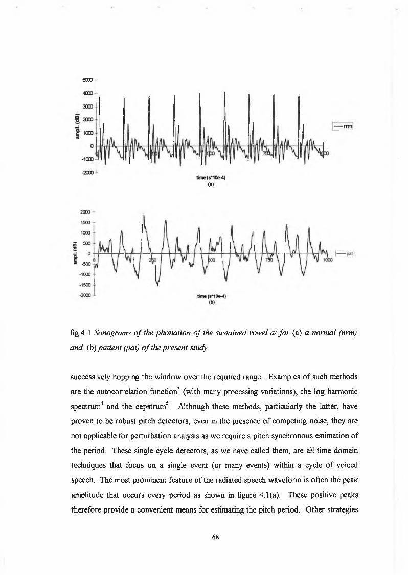
5000

(a)

fig.4.1 Sonograms o f the phonation o f the sustained vowel a / fo r (a) a normal (nrm)

and (b) patient (pat) o f the present study

successively hopping the window over the required range. Examples o f such methods

are the autocorrelation function3 (with many processing variations), the log harmonic

spectrum4 and the cepstrum5. Although these methods, particularly the latter, have

proven to be robust pitch detectors, even in the presence o f competing noise, they are

not applicable for perturbation analysis as we require a pitch synchronous estimation of

the period. These single cycle detectors, as we have called them, are all time domain

techniques that focus on a single event (or many events) within a cycle o f voiced

speech. The most prominent feature o f the radiated speech waveform is often the peak

amplitude that occurs every period as shown in figure 4.1(a). These positive peaks

therefore provide a convenient means for estimating the pitch period. Other strategies

68

involve taking the negative peaks from the waveform. Low pass filtering the waveform

at a frequency between the fundamental frequency (fD) and twice the fundamental and

calculating the zero-crossing rate is another popular method. An output radiated

speech waveform and it’s low pass filtered version are shown in figure 4.2. Another

strategy involves matching the waveform from cycle to cycle, usually implemented

through some form of least squares estimation procedure6. The issue as to which

method gives the most reliable results has been addressed in detail by several

researchers along with other methological concerns7,8,9.

fig.4.2 110 Hz synthesis file (original) and a filtered version which has been low

passed at 1.5 times an initial fO estimate

Although Titze et al8 have shown waveform matching to be a robust method of pitch

extraction even in the presence o f additive noise and low level frequency and amplitude

modulations, the method becomes sensitive to frequency modulations exceeding six

percent and hence, in anticipation o f fluctuations o f this magnitude in respect o f

pathological voices the method was not implemented. However, in recognition o f the

robustness o f the method i.e. many estimates are obtained per cycle, a low pass version

of waveform matching was developed. Three further methods using the positive peaks

from the original and low passed waveforms and the positive zero crossings from the

low passed waveform were also implemented. The analysis details for the three

methods based on the low passed waveform are shown in A, B and C.

69

A. Waveform Matching of the Low Passed Filtered Waveform

In this method an initial estimate of the fundamental frequency (fO) is obtained using

any convenient short term fO extraction method, the cepstrum being chosen here.

Following this initial fO estimate, the waveform is low passed filtered at 1.5xf0 using a

250th order, low pass, finite impulse response (FIR) filter (Matlab’s signal processing

toolbox). As a consequence of this filtering the low passed waveform will only cross

the x-axis twice per cycle, giving one positive (PZC) and one negative zero crossing

(NZC) per cycle as shown in fig. 4.3. The negative zero crossings (NZC) are then used

as rough period markers with respect to which the search for cyclic events begins. Any

prominent event within the pitch markers is taken as the starting point for the

waveform matching. The negative peak location ‘NP(1)’ was chosen in this

implementation (fig.4.3). A point ‘NP(2)’ between the second and third rough markers

is then found such that the mean squared error between the adjacent wavefroms is

minimal. The pitch period is hence calculated to be ‘NP(1)-NP(2)\

fig. 4.3 L o w p a s s e d ( 1 . 5 > f0 ) f i l t e r e d w a v e f o r m w i t h n e g a t i v e p e a k (N P ) , p o s i t i v e p e a k

( P P ) , p o s i t i v e z e r o c r o s s i n g ( P Z C ) a n d n e g a t i v e z e r o c r o s s i n g ( N Z C ) p i t c h m a r k e r s .

The exact method can be followed from the five steps below with reference to figure

4.3, which is essentially the same approach that Titze et al used on the original

waveform.

70

1. The rough markers are set using the negative zero crossings o f the low passed

filtered waveform (NZC(l) and NZC(2)).

2. The negative peak (NP(1)) between NZC(l) and NZC(2) is located.

3. An initial guess is made of the negative peak location between the second and third

rough markers NP(2) = NZC(2)+( NP(1)-I(1)) (see fig.4.3).

4. A search limit o f a user given percentage, PERC (typically 15-30%) is set such that

J1 = NP(1) - PERC * (NP(2)-NP( 1))

J2 = NP(1) + PERC*(NP(2)-NP(1))

and a point Jm between J1 and J2 is found so that ERR(Jm) is minimal, where

1 -*-1ERR(Jm) = . _ x X (buff(k + 0 - NP(i -1 )]) - buff(k)) eqtn.4.1

J J N r ( J 1 J k = P ( i - i )

where ‘buff is the data buffer.

5. The resulting estimate of pitch period is limited by the sampling frequency and hence

interpolation is used to improve the estimate. A second order polynomial is fitted to

the points ERR(Jm-l), ERR(Jm) and ERR(Jm+l) to find the minimal location J'.

6. The period is hence given as NP(2)= NP(1)-J'

7. The process is similarly repeated for all periods of the waveform.

B. Positive Peaks from the Original and Low Passed Waveforms

Again, rough period boundary markers are set as for the waveform matching method.

Then the positive peak locations (PP(i)) are found within these markers using a simple

peak picking algorithm. Interpolation is then used to obtain a more accurate estimate

o f the peak location using a second order polynomial as follows

™ - 0.5 x (buff(PPi +1) - buff(PPi -1 ))1 + buff(PPi +1) - 2 x buff(PPi) + buff(PPi - 1 ) Cqtn' ’

71

where ‘buff specifies the signal array.

C. The Zero Crossing Method

Zero crossing can only be used on a low pass filtered version o f the output radiated

speech waveform unless o f course a contact microphone or electroglottography (EGG)

was used to record the signal in which case the original waveform can be analysed

directly. The rough period markers are set as before using the negative zero crossing

locations. The positive zero crossings (PZC) are then located between these markers

(fig.4.3) and a first order polynomial (i.e. straight line interpolation - equation 4.3) is

fitted in order to improve the estimate.

- buff(PZC>)PZC<,) = PZCi + bufffpZCj + 1)_ buff(pzCi) eqtn.4.3

where again ‘buff indicates the signal.

The i*11 fundamental frequency is hence calculated as follows

fsamft>(i) = — eqtn.4.4

w PZC(i + 1 ) - PZC(i) 4

where fsam is the sampling frequency.

4.2.1 Test Stimuli

In order to test the accuracy o f the pitch extraction and subsequent perturbation

analysis programs it is important to have precise knowledge of the accuracy obtainable

with the synthesis data. Therefore, some further comments on the jittered synthesis

data which were introduced in chapter 2 are given. In the synthesis we have simulated

two very different conditions o f jitter, random and cyclic. The former case, which is

72

perhaps the more common simulation, is produced using a random number generator

as shown

fsamP 1 = T T ’

PI x (100 + per x randn)P = ^ - eqtn.4.5

100 H

PI = pitch period, fsam = sampling frequency, fO = fundamental frequency

randn = normally distributed random numbers, mean zero, variance one

per = percentage perturbation

The user inputs fO, from which the pitch period is simply obtained as shown in

equation 4.4. Pitch perturbations of variance ‘per’ are then introduced via Matlab’s

random number generator ‘randn.m’ which produces normally distributed random

numbers with mean zero and variance one. For example, setting per = 4, gives a jitter

set with a standard deviation of 4%. This pitch period variation is plotted with respect

to time in fig. 4.4. However, our data are also constrained by the fact that they must

be integer valued. The function round.m is used to round the data to the nearest

integer value. This must be imposed because alternatively the data takes the ‘floor’

integer value by default.

p e r i o d n o

fig.4.4 V a r i a t i o n o f p i t c h p e r i o d f o r t h e 4 % s td . d e v . r a n d o m j i t t e r s i g n a l w i t h a n d

w i t h o u t r o u n d i n g t o t h e n e a r e s t i n t e g e r .

73

The glottal period was varied so as to keep the relative harmonic levels equal i.e. all

components were scaled in such a way so as to match a given period and this put

further restrictions on the data, requiring integer values for the rise time (Nl) and

closing time (N2) of the glottal pulse. The synthesis data were produced in such a way

so as to represent a 10 kHz sampling frequency and the jitter set signals were

investigated using the 110 Hz files. The equivalent pitch period is -9.1 ms or 91

sample points when rounded. It can be seen therefore (fig.4.4) that when low level

pitch perturbations are introduced through the random number generator, they are only

very crudely approximated when rounded to the nearest integer.

The cyclic jitter values were produced by simply alternating successive periods between

PI and P2 where PI and P2 are fixed. The spectral consequence of this is to produce

an harmonic peak at an octave lower in the frequency spectrum (fig. 4.5).

-160

frequency (Hz)

fig.4.5 S u b - h a r m o n i c r e g i m e i n t r o d u c e d a s a r e s u l t o f th e c y c l i c j i t t e r p e r t u r b a t i o n

This may seem like a very unnatural way in which to introduce jitter but in

consideration of how one glottal cycle can influence the next it may in fact be a more

realistic manner in which to simulate jitter in certain cases of vocal pathology e.g. fry

phonation. Some work has been done in respect to what the distribution of jitter

actually follows (Pinto et al10) in cases of normal and pathological speakers. The data

set for normals produce a somewhat Gaussian distribution, although some degree of

skewness is apparent. The distribution involving cases with vocal pathology depends

on the type of the pathology with diplophonia, for example giving a bimodal

distribution.

74

4.2.2 Results of the Various Extraction Procedures

Having detailed the jitter signals in the previous section we are now in a position to

appreciate the results that are returned from the fO extraction procedures. The next

section gives a detailed account o f the various pitch perturbation measurements that

have been developed in order to assess the periodicity o f the speech signal. We shall

use one o f these, the perturbation index defined as

1 ^ fO(i + l)-fO (i)PF1 = T ^ x 100 eqtn.4.6

0.5 x [(fD(i +1) + f0(i))]

(where N is the total number o f periods), in order to compare the different extraction

procedures and, after choosing the most appropriate extraction method, we compare

the usefulness o f the different perturbation measurements. Equation 4.6 is called the

‘Pitch Perturbation Factor One’ (PF1). This value (for the output radiated speech

waveform) is plotted in per cent versus random pitch perturbation and cyclic pitch

perturbation of the glottal source in fig.4.6 and fig.4.7.

-pp-ppi-wav

-pzc

source period perturbation (std. dev. in %)(a)

fig.4.6 PF1(%) values for random jitter using the four extraction methods where PP-

positive peaks, PPl-positive peaks o f low passed filtered waveform, wav-waveform

matching and PZC-positive zero crossing

75

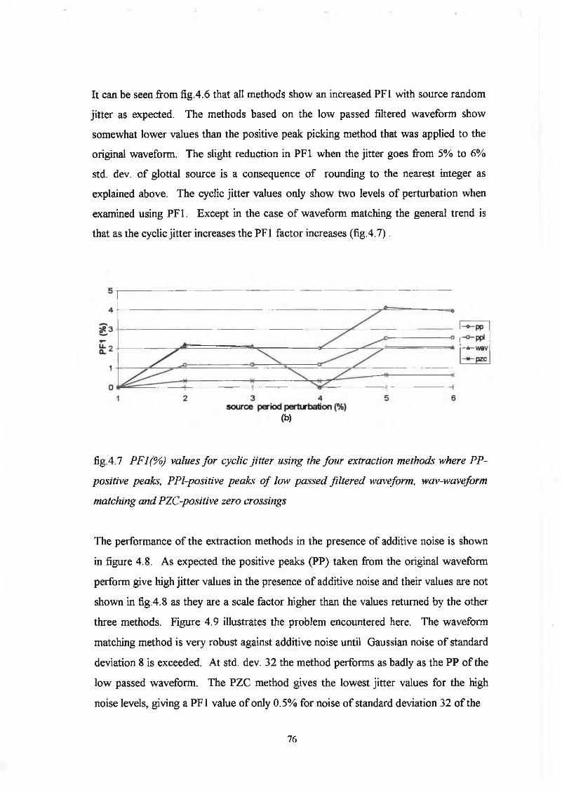
It can be seen from fig.4.6 that all methods show an increased PF1 with source random

jitter as expected. The methods based on the low passed filtered waveform show

somewhat lower values than the positive peak picking method that was applied to the

original waveform. The slight reduction in PF1 when the jitter goes from 5% to 6%

std. dev. of glottal source is a consequence of rounding to the nearest integer as

explained above. The cyclic jitter values only show two levels of perturbation when

examined using PF1. Except in the case of waveform matching the general trend is

that as the cyclic jitter increases the PF1 factor increases (fig.4.7).

(b)

fig.4.7 P F 1 ( % ) v a l u e s f o r c y c l i c j i t t e r u s i n g t h e f o u r e x t r a c t i o n m e t h o d s w h e r e P P -

p o s i t i v e p e a k s , P P l - p o s i t i v e p e a k s o f l o w p a s s e d f i l t e r e d w a v e fo r m , w a v - w a v e f o r m

m a t c h i n g a n d P Z C - p o s i t i v e z e r o c r o s s i n g s

The performance of the extraction methods in the presence of additive noise is shown

in figure 4.8. As expected the positive peaks (PP) taken from the original waveform

perform give high jitter values in the presence of additive noise and their values are not

shown in fig.4.8 as they are a scale factor higher than the values returned by the other

three methods. Figure 4.9 illustrates the problem encountered here. The wavefonm

matching method is very robust against additive noise until Gaussian noise of standard

deviation 8 is exceeded. At std. dev. 32 the method performs as badly as the PP of the

low passed waveform. The PZC method gives the lowest jitter values for the high

noise levels, giving a PF1 value of only 0.5% for noise of standard deviation 32 of the

76

additive noise at glottal source (std. dev. %)

—®—ppl-o -w a v- * - p z c

fig.4.8 P F 1 ( % ) v a l u e s f o r a d d i t i v e n o i s e u s i n g th e f o u r e x t r a c t i o n m e t h o d s w h e r e P P -

p o s i t i v e p e a k s ( o f f s c a l e ) , P P l - p o s i t i v e p e a k s o f lo w p a s s e d f i l t e r e d w a v e f o r m , w a v -

w a v e f o r m m a t c h i n g a n d P Z C - p o s i t i v e z e r o c r o s s i n g s

fig. 4.9 S p e e c h w a v e f o r m w i t h a d d i t i v e n o i s e ( s td . d e v . 1 6 % ) i l l u s t r a t i n g w h y p o s i t i v e

p e a k p i c k i n g g i v e s h i g h j i t t e r s c o r e s

glottal source. However the jitter values obtained by this method are not as low as the

waveform matching values for lower levels of additive noise.

Figure 4.10 shows the effect of shimmer on the jitter values. All methods based on low

pass filtering the waveform perform extremely poorly for the shimmer signals with

jitter values of over 5 % for glottal source amplitude perturbation signals with a

variance of 32. The PZC method performs somewhat better but still gives a PF1 value

77

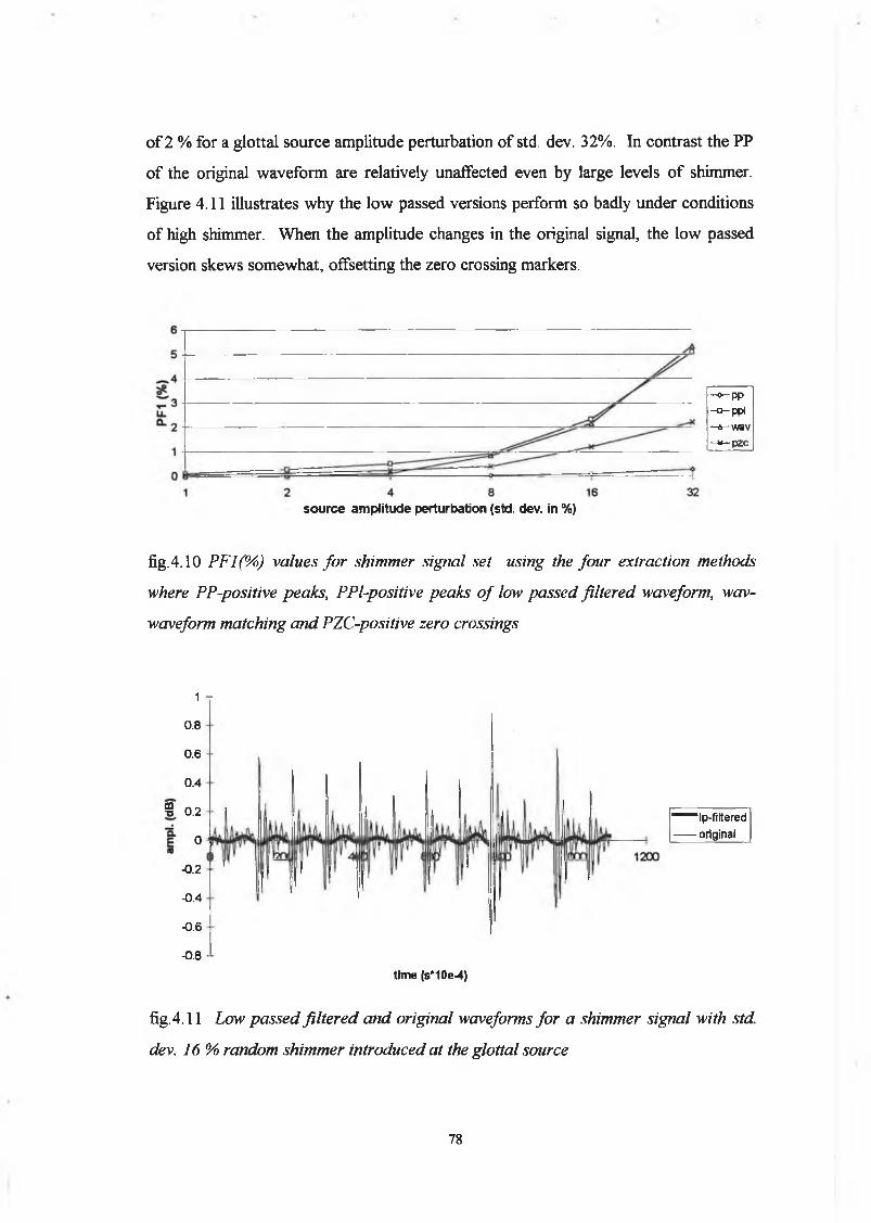
of 2 % for a glottal source amplitude perturbation of std. dev. 32%. In contrast the PP

of the original waveform are relatively unaffected even by large levels of shimmer.

Figure 4.11 illustrates why the low passed versions perform so badly under conditions

of high shimmer. When the amplitude changes in the original signal, the low passed

version skews somewhat, offsetting the zero crossing markers.

source amplitude perturbation (std. dev. in %)

-o -P P-o -p p l- a- wav -*-pzc

fig.4.10 P F 1 ( % ) v a l u e s f o r s h i m m e r s i g n a l s e t u s i n g t h e f o u r e x t r a c t i o n m e t h o d s

w h e r e P P - p o s i t i v e p e a k s , P P l - p o s i t i v e p e a k s o f lo w p a s s e d f i l t e r e d w a v e fo r m , w a v -

w a v e f o r m m a t c h i n g a n d P Z C - p o s i t i v e z e r o c r o s s i n g s

a■a

1 t

0.8

0.6

0.4

0.2

0

- 0.2

-0.4

-0.6

-0.8 --

“ ^ Ip -filte re d

original

time (s*10e-4)

fig. 4.11 L o w p a s s e d f i l t e r e d a n d o r i g i n a l w a v e f o r m s f o r a s h i m m e r s i g n a l w i t h s td .

d e v . 1 6 % r a n d o m s h i m m e r i n t r o d u c e d a t t h e g l o t t a l s o u r c e

78

Also of interest are the jitter values obtained for the radiated output as compared to the

jitter values obtained for the glottal source signals. Figure 4.12 shows this relation

between source and output jitter values for the extraction method that gave the lowest

level of jitter for that perturbation. For the shimmer signal set, the increased levels of

jitter (where the fundamental frequency was obtained using any of the low pass filtered

extraction procedures) for the output radiated waveforms are simply due to the overall

multiplicative effect of the vocal tract filter function.

—*-s 1 1 0 a r -p -g 1 1 0 a r

2 3 4 5pitch perturbation of glottal source (std. dev. %)

(a)

2 4 8 16additive noise of glottal source (std. dev. %)

(b)

amplitude perturbation of glottal source (std. dev. %)

-o-s110s-o-g110s

fig.4.12 P F 1 v a l u e s f o r s o u r c e a n d r a d i a t e d w a v e f o r m s f o r (a ) r a n d o m j i t t e r (b )

a d d i t i v e n o i s e a n d ( c ) a m p l i t u d e p e r t u r b a t i o n ( g - g l o t t a l s - o u t p u t r a d i a t e d s p e e c h )

79

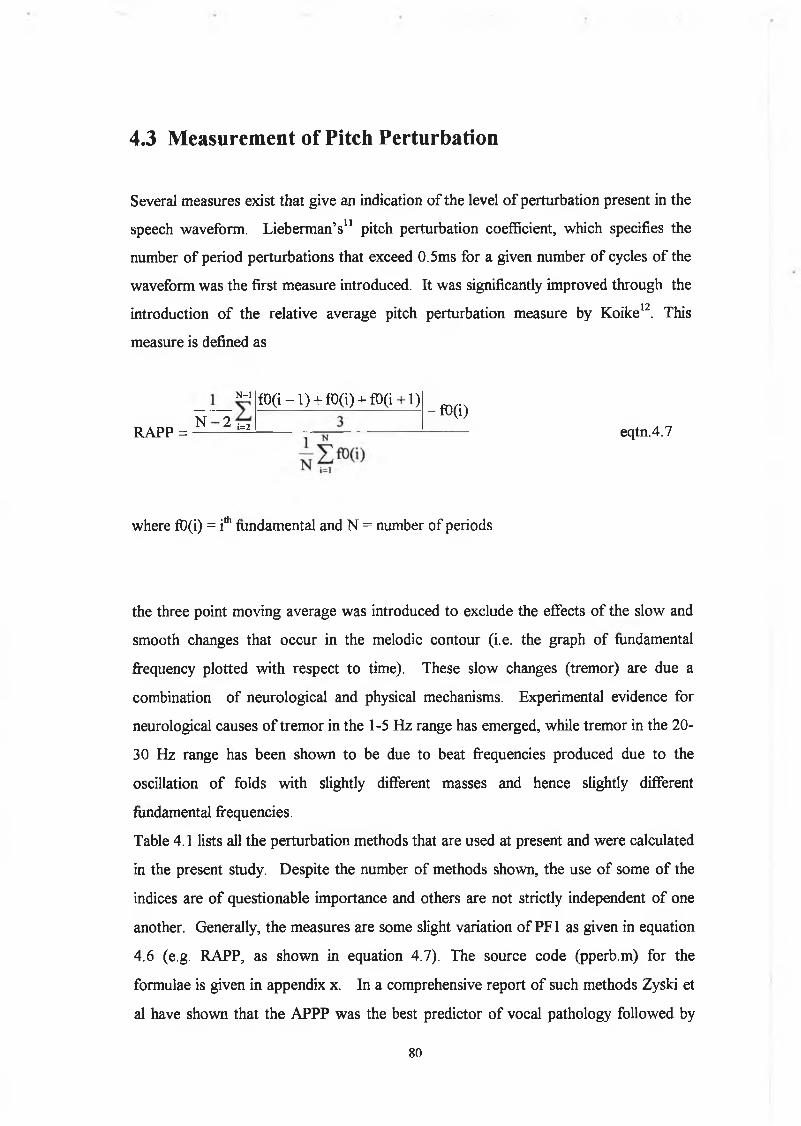
4.3 M easurem ent o f Pitch Perturbation

Several measures exist that give an indication o f the level o f perturbation present in the

speech waveform. Lieberman’s11 pitch perturbation coefficient, which specifies the

number of period perturbations that exceed 0.5ms for a given number of cycles o f the

waveform was the first measure introduced. It was significantly improved through the

introduction o f the relative average pitch perturbation measure by Koike12. This

measure is defined as

N - l

RAPP = N 2 1=2

f0( i - l ) + f0(i) + f0(i + l)- f 0(i)

eqtn.4.7

where f0(i) = i* fundamental and N = number o f periods

the three point moving average was introduced to exclude the effects o f the slow and

smooth changes that occur in the melodic contour (i.e. the graph of fundamental

frequency plotted with respect to time). These slow changes (tremor) are due a

combination o f neurological and physical mechanisms. Experimental evidence for

neurological causes o f tremor in the 1-5 Hz range has emerged, while tremor in the 20-

30 Hz range has been shown to be due to beat frequencies produced due to the

oscillation o f folds with slightly different masses and hence slightly different

fundamental frequencies.

Table 4.1 lists all the perturbation methods that are used at present and were calculated

in the present study. Despite the number of methods shown, the use o f some o f the

indices are o f questionable importance and others are not strictly independent o f one

another. Generally, the measures are some slight variation of PF1 as given in equation

4.6 (e.g. RAPP, as shown in equation 4.7). The source code (pperb.m) for the

formulae is given in appendix x. In a comprehensive report o f such methods Zyski et

al have shown that the APPP was the best predictor of vocal pathology followed by

80

RAPP. Askenfelt et al13 also carried out a test comparing seven different perturbation

measures and found that the standard deviation of the distribution of the relative

frequency differences was the

PERTURBATION MEASURE ABBREVIATION

Average pitch perturbation APP

Relative Average pitch perturbation RAPP

Average percentage pitch perturbation APPP

Normalised std.dev. pitch stdndfO

Mean 1st order perturbation PF1

Mean 2nd order perturbation PF2

Directional perturbation factor DPF

Normalised std.dev. of 2nd order pert stdnd2f0

Std.dev. of pitch perturbation stddfO

Table 4.1 P i t c h P e r t u r b a t i o n M e a s u r e s ( s o u r c e c o d e - A p p e n d i x A ( p p e r b .m ) )

most useful acoustic measure for use in clinical applications. This standard deviation is

a measure of the DFO distribution, where DFO = (Fn+1 - Fn)/Fn . An example of such

a distribution is shown in figure 4.13 for a normal and pathologic speaker.

■ 1 l -0 0 1 0 0

B n r m ■ p a t

fig.4.13 H i s t o g r a m o f t h e d i f f e r e n c e i n f O (d fO ) d i s t r i b u t i o n f o r a p a t i e n t a n d n o r m a l

o f t h e p r e s e n t s t u d y

As stated in section 4.2.2 Pinto et al have also investigated the distribution o f

perturbation measures and have attempted to unify the classification o f perturbation

measures through the use o f forward and backward difference equations. We have

followed their recommendation that fundamental frequency as opposed to pitch period

be used when investigating jitter and all the jitter perturbations used in this study were

calculated using the fundamental frequency as opposed to the pitch period. The

variation o f four pitch perturbation measures with respect to the four different source

perturbations are shown in fig.4.14(a,b,c,d). All measures are shown to give essentially

the same information with PF1 and APPP being essentially the same index.

Cyclic Jitter (%)(a )

■rapp

' Pf2 ■appp -pf1

&c3.dfe­rno.En

-ra p p

-p f2

-a p p p

- Pf1

pitch perturbation o f glottal source (std.dev.%) (b)

- © - r a p p - o - p f 2

—a - a p p p

~x~pf1

82

0.4 ■

Ig 0.3xijo. 0.2a.E 0.1a

0»1

fig.4.14 V a r ia t io n o f f o u r p i t c h p e r t u r b a t i o n m e a s u r e s ( R A P P , P F 2 , A P P P a n d P F 1 )

w i t h r e s p e c t t o t h e f o u r s o u r c e p e r t u r a b t i o n m e a s u r e s o f ( a ) c y c l i c j i t t e r (b ) r a n d o m

j i t t e r ( c ) s h i m m e r a n d ( d ) a d d i t i v e n o i s e

Up until now we have only considered the indices as showing general trends. However

the idea o f using the indices is to introduce accurate, quantifiable measures of

aperiodicity. Therefore, if our signal is synthesized with 6% jitter then a first order

measure should show 6% jitter or else there is an error in the tracking or the index.

The first requirement o f our pitch tracker is that it should follow the changes in fO

perturbation accurately. However, as we have seen in section 4.2, no method follows

the jitter increase in a linear fashion as we might have expected. The reason for this is

not so much due to any limitations o f the pitch trackers or indices but is more a

consequence o f the scaling and integer requirements o f the glottal pulses as mentioned

above. This point is illustrated with the cyclic jitter values. Fig.4.7 shows 3 levels of

jitter which are given here in tabular form (Table.4.2). Therefore caution must be

taken when interpreting the indices returned from a given extraction procedure for the

synthesis files o f given jitter levels (i.e. the discrepancy between values has arisen due

to the constrains o f the synthesis files as opposed to any limitations o f the pitch

trackers or perturbation indices). Keeping all parameters in the glottal model scaled

accurately can only be achieved by increasing the sampling frequency. A simpler

approach would be to simply truncate the closed phase. Although, this is not the

desired approach from the spectral characterisation viewpoint, it does provide a simple

means o f assessing the accuracy o f pitch extraction procedures in a consistent manner.

83

1 EXTRACTION

METHOD/

SYNTHESIS

FILE

POSITIVE

PEAKS

(PP)

(% JITTER)

POSITIVE

PEAKS

LOW

PASSED-PPL

(% JITTER)

POSITIVE

ZERO

CROSSINGS

(PZC)

(% JITTER)

ACTUAL

SYNTHESIS

VALUE

(% JITTER) ;

sll0jp6 3.93 2.55 0.62 6.39 |

gll0jp6 4.12 1.90 0.89

sll0jp5 4.12 2.17 0.67 5.35

gl 10jp5 4.17 2.17 0.79

sll0jp4 2.01 1.17 0.32 4.3

gl 10jp4 2.10 0.94 0.41

sll0jp3 2.04 1.15 0.33 3.24

gl 10jp3 2.13 1.01 0.41

gl 10jp2 2.20 1.05 0.34 2.17

sll0jp2 2.15 0.95 0.41

gllOjpl 0 0 0 1.09

sllOjpl 0 0 0

Table 4.2 C y c l i c j i t t e r v a l u e s f o r t h e s o u r c e a n d r a d i a t e d w a v e f o r m s f o r a l l e x t r a c t i o n

p r o c e d u r e s c o m p a r e d t o a c t u a l s y n t h e s i s v a l u e f o r c y c l i c j i t t e r ( r i g h t h a n d c o lu m n ) .

fig.4.15 I n t e g e r c o n s t r a i n t o n s c a l i n g o f g l o t t a l p u l s e m o d e l f o r 6 % c y c l i c j i t t e r

The integer constraints only apply to the jitter set synthesis data and therefore the

measurement of jitter in the presence of noise or shimmer can be taken as accurate.

84

4.4 M easurem ent o f Am plitude Perturbation

The measurement o f amplitude perturbation has also received considerable attention in

the literature. The Zyski et al review is based on measurements that were taken from

speech samples recorded using a contact microphone in which the amplitude o f the

resultant waveform is somewhat more directly related to the glottal waveform than

when simply using the standard audio microphone. Gauffin and Sundberg14 have

shown that the peak amplitude o f the flow glottogram waveform is in fact related more

closely to the amplitude o f the fundamental in the glottal source spectrum than to the

overall intensity o f the speech waveform and that the negative peak amplitude of the

differentiated flow glottogram shows a high correlation with sound pressure level.

Therefore the peak (or rms, if we consider the waveform to be quasi-periodic)

amplitude in the output radiated speech waveform can be considered to relate more

closely to the peak to peak o f the differentiated flow glottogram signal than the peak

flow o f the glottogram signal. Furthermore, Hillenbrand has shown that the same

shimmer levels result for synthesis data with jitter, shimmer and additive noise

perturbations, regardless o f whether peak or rms amplitudes o f the output radiated

speech waveform were used. As shown in figure 4 .16(a) values for measured shimmer

reflect well the source amplitude perturbation. In a) the HPF1 measure, defined as

„ 1 ^ Hf(i + 1 )-H f(i)HPF1 = --------/ x 100 eqtn.4.8

N - l t ? 0 .5 x [ ( H f ( i + l) + Hf(i))] 4

H f = peak amplitude o f waveform within a cycle

N = total no. o f periods

or in words, the variation in peak amplitude of the waveform from cycle to cycle,

divided by the amplitude o f the waveform shows good correlation with the source

amplitude perturbation levels. The effect o f the vocal tract filter function does not alter

the amount o f shimmer measured. This implies a direct correlation between the peak in

85

-81108-g110s

Random source shimmer (std dev %)(a)

- * -s 1 1 0 a r-o -g 110ar

4 8 16source additive noise (std. dev. %)

(b)

Q-X

-s110jj-g i l0 j

pitch perturbation of glottal source (std. dev. %) (c)

fig.4.16 A m p l i t u d e p e r t u r b a t i o n f a c t o r o n e ( H P F 1 ) v s (a ) s h i m m e r , ( b ) a d d i t i v e n o i s e

a n d (c ) r a n d o m j i t t e r

the source model and the peak in the output radiated speech waveform. Part b) of the

figure shows that shimmer measures (HPF1) are very sensitive to random noise

introduced at the glottal source. Also note that the source amplitude perturbation

increases in a regular fashion whereas the vocal tract filtered waveform’s amplitude

perturbation is somewhat less regular. Part c) of the figure shows the amplitude

perturbation measure plotted with respect to jitter. For the source signal, jitter has

86

very little effect on amplitude perturbation. However, for the filtered signal there is a

marked effect on the amplitude perturbation, and in contrast to the jitter measurements

obtained in the presence of shimmer, which were due to the measurement technique

rather than increased aperiodicity o f the signal, the amplitude perturbation

measurement reflects an actual increase in shimmer. This is due to the source filter or

harmonic formant interaction as stated by Imaizumi15. As the source period changes,

the vocal tract filter is excited with different harmonic frequencies, therefore receiving

different resonance contributions and hence differences in the amplitude o f the

waveform from period to period. A list o f shimmer values that were evaluated in the

present study are shown in table 4.3. There is a one to one correspondence with the

pitch perturbation values, except for a further dB measure included in table 4.3. The

same comments noted for the jitter measures are also true for the shimmer measures

listed here.

PERTURBATION MEASURE ABBREVIATION

Average amplitude perturbation AAP

Relative Average ampi. Perturbation RAAP

Average percentage ampi, perturbation APAP

Normalised std.dev. amplitude stdndHfO

Mean 1st order perturbation HPF1

Mean 2nd order perturbation HPF2

Directional perturbation factor DHPF

Normalised std.dev. o f 2nd order pert. stdndH2fO

Std.dev. o f ampi. Perturbation stddHfl)

Average power difference (shimmer) dBdHfO

Table 4.3 Amplitude perturbation measures (source code- appendix A (amperb.m))

In recognition o f the fact that the various jitter and shimmer indices represent basically

the same information, only the pitch perturbation factor one (PF1) and amplitude

perturbation factor one (HPF1) are shown for the patient and normal data fig.4.17(a,b).

87

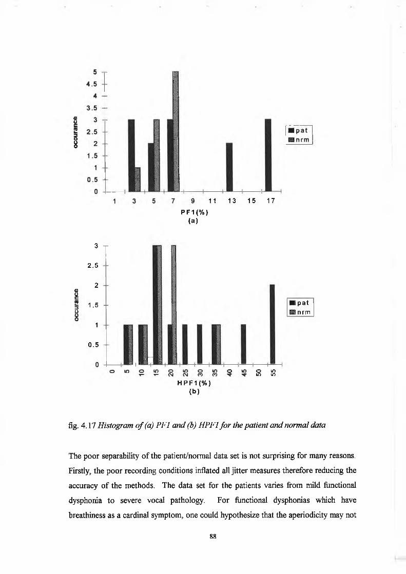
0o

o8

11 13 15 17

P F1 (%) (a)

0)o

3 T

2 .5

2

i 1.5 + o

1

0.5

:<■ a«+■

H P F1(%) (b)

I pat I nrm

o in oIf) min

fig. 4.17 Histogram o f (a) PF1 and (b) HPF1 fo r the patient and normal data

The poor separability o f the patient/normal data set is not surprising for many reasons.

Firstly, the poor recording conditions inflated all jitter measures therefore reducing the

accuracy o f the methods. The data set for the patients varies from mild functional

dysphonia to severe vocal pathology. For functional dysphonias which have

breathiness as a cardinal symptom, one could hypothesize that the aperiodicity may not

88

increase to any great extent. Due to the more sinusoidal nature o f the waveform

(although aspiration noise is also present), waveform matching methods may show

lower levels o f jitter than for the more complex ‘normal’ waveforms. However, five

of the thirteen samples from the patient data set show a clear difference in PF1 to the

normal data set and are from patients with severe organic vocal pathology. Note the

values for PF1 range from 1 to 7 % for the normals in this study, whereas Horii16 has

stated that 0.1 to 1% perturbation are in the range o f normal. Although we have

chosen the variation o f fundamental frequency as opposed to pitch period in the

evaluation o f jitter, the PF1 measure is a time-frequency invariant measurement as

indicated by equation 4.9

AfO AT—— = — eqtn.4.9fO T

and as such can not be considered to be a cause o f the above discrepancy. The

difference is due to poor quality tape recording as mentioned above, which has been

shown to significantly increase jitter values (2 refs). The effect o f the poor quality

recording is particularly strong here as the recorder exhibited a strong “Watergate

Buzz” (i.e. mains frequency and odd integer harmonics) in it’s frequency response

characteristic. In an effort to remove these unwanted artifacts, all speech signals were

high pass filtered at 60 Hz using a Ramiz filter. More sophisticated methods, that

remove the higher harmonic noise components using comb filtering have also been

developed for this purpose.

4.5 A utocorrelation and Correlation Analysis

Many other time domain methods exist other than those mentioned above in respect to

perturbation analyses. In fact in chapter 5 the harmonic to noise ratio is calculated

using an adaptation o f Yumoto’s time domain signal to noise ratio estimate17.

89

Kasuya’s time domain filter18, again providing an harmonic to noise ratio estimate was

also programmed and the source code is given in appendix.x. The peak to mean o f the

output waveform value was also suggested as a useful measure by Klatt et al19 and

Fant20 has shown that the bandwidth of the first formant can also be estimated from

calculations performed on the output waveform.

Another popular time domain method is the correlation or autocorrelation function,

defined as

N—1

Coring, h)j = 2 S +khk’ eqtn.4.10k = 0

g,h are periodic with period N.

gk=hjc for autocorrelation.

This measures the similarity o f the waveform from period to period. A property o f the

autocorrelation function is that if the function being correlated is periodic then the

autocorrelation is also period with the same frequency. This property has been

successfully used in order to provide accurate pitch estimation. Rabiner gives an

extensive list o f processing details in order to enhance the pitch estimate using the

autocorrelation function. A program was written in order to implement this estimate

(timepit.m) but our main concern here is the use o f the correlation function for

providing a similarity index as opposed to a pitch estimate. The basic idea, as

introduced by Hillenbrand is that a waveform with good periodicity exhibits strong

similarity between adjacent cycles and hence will have a high correlation index. In the

program implemented here, the correlation index proposed by Hillenbrand21 (XCP) and

anew measure (MM2) were calculated for the original and low and band pass versions

o f the original waveforms. The method involves taking the correlation o f the original

waveform with a delayed copy o f itself at delays between the maximum and minimum

expected pitch period (3.3ms and 16.7 ms were used). For periodic signals a peak

occurs in the correlation function at a delay corresponding to the fundamental period.

As the correlation peak is dependent on the signal amplitude a normalisation scheme is

required. Two normalised correlation indices were calculated every 10 ms using a 30

ms analysis frame. The first was the standard measure of the peak in the

90

■ pat H n r m

M M 2 ( a r b . u n i t s ) (b)

■ pat @nrm

fig.4.18 Histogram o f correlation indices (a) XCP and (b) MM2 fo r normal and

patient data sets

autocorrelation function (XCP), the second was calculated by simply taking the

standard deviation o f the difference between waveforms when the overlap

corresponded to the peak in the autocorrelation function (MM2). The performance of

the two measures with respect to the patient/normal data set is shown in fig. 4.18. As

can be seen in the figure, the measures show a strong overlap between the patient and

normal data sets.

91

4.6 Discussion/Conclusion :

In attempting to provide objective acoustic indices o f vocal pathology based on time

domain analysis methods the main thrust has been towards extracting measures o f pitch

and amplitude perturbation. The original strategy was firstly to find a pitch extraction

method that gives reliable pitch estimates in the presence o f additive noise and shimmer

and then to investigate the nature o f the perturbation by choosing suitable perturbation

indices from the list given in table 4.1. However, we have shown that different pitch

extraction methods perform better depending on the source perturbation present.

When shimmer is present the method giving the lowest jitter index is the positive peaks

from the original waveform. When random noise is added to the source signal using

the positive peaks to extract the pitch period gives veiy high jitter values. Conversely,

the positive zero crossing o f the low pass waveform give robust pitch estimates in the

presence o f additive noise and poor estimates in the presence o f shimmer. Therefore a

comparison of the jitter indices returned from different extraction methods could

possibly provide information regarding the source o f the perturbation. The results for

the waveform matching (low passed) are o f considerable interest (fig. 4.8). The least

squares error estimate o f waveform matching reported by Titze et al9 only examines

waveforms with a minimum of 10 dB signal to noise ratio. However, signal to noise

ratios for pathological voices would be expected to fall below this value. Fig.4.8

shows that the waveform matching is very robust up until std. dev. 8 % (~ 15 dB -

output file) additive noise but once this value is exceeded the method rapidly

deteriorates with positive zero crossings showing considerably lower jitter values. This

suggests that the waveform matching method of pitch extraction may not be the most

applicable technique to use on pathological voice types.

Furthermore, it has been shown that although several pitch and amplitude perturbations

measures exist many are redundant or offer no new information regarding the signal.

Despite this fact, different (new) perturbation measures may be useful in differentiating

perturbation types. For the cyclic and random jitter signals of the present study, a

simple second order perturbation measure subtracting every second period reveals

92

which type of perturbation is present. The original intention of introducing these files

was to show that for a given % pitch perturbation, the spectral characteristics can be

quite different and therefore a perturbation o f a given value could arise due to very

different vibratory characteristics o f the vocal folds. This index comparison could not

be tested due to the limitations o f the jitter synthesis data as stated. There are further

considerations to bear in mind in considering cyclic jitter in pathological voice types

(e.g. vocal creak). For the synthesis data it was known a priori what the actual

fundamental was and filtering began at 1.5 times this value but for real data our pitch

trackers could easily chose ‘two cycles’ as the fundamental and therefore give zero

perturbation indices. Further work is required to produce useful perturbation indices

under these conditions. In regard to jitter measurements in the presence of additive

noise and shimmer we have shown that the increase in jitter is due to measurement

error that arises due the presence o f these perturbations. In respect o f the low pass

results for shimmer, a simple normalisation scheme would perhaps solve this problem.

However in the case o f shimmer in the presence o f jitter we have shown the increase in

shimmer to be a result o f the source filter interaction as a result o f different

fundamental frequencies exciting the vocal tract. Also, we have shown that shimmer

measurements are more strongly affected by additive noise than actual shimmer levels

present in the signal. A more robust correlation measure would be obtained if it

compared not only adjacent periods o f the waveform but also the first (then second

etc) with the third, fourth etc. until the complete time record is finished. Presently used

indices based on commercially available speech software packages “cannot reliably be

applied to voices that are even mildly aperiodic”. The conclusion reached from this

study is that present perturbation indices have some utility but that the measures could

be greatly advanced through careful consideration o f the extraction procedures used

along with the implementation o f new indices based on a knowledge of vibratory

characteristics.

93

4.7 Bibliography

1. Zyski, BJ. et al Perturbation analyses o f normal and pathologic larynges. Folia

phoniat. 1984, 36: 190-198

2. Hess, W. Pitch determination o f speech signals, algorithms and devices. Berlin,

Heidelberg: Springer Verlag, 1983

3. Rabiner, LR. On the use o f autocorrelation for pitch detection. IEEE Trans.

Acoust. Speech and Sig. Processing, 1977; ASSP-25: 24-33

4. Rabiner, L. and Schafer, R. Digitial processing o f speech signals, Englewood Cliffs,

N.J.: Prentice Hall, 1978

5. Deller, J. Proakis J. and Hansen, J. Discrete time processing of speech signals, NY:

Macmillan, 1989

6. Milenkovic, P. Least mean square measures o f voice perturbation. J. Speech and

Hear. Res. 1987, 30: 529-538

7. Deem, JF. et al The automatic extraction o f pitch perturbation using

microcomputers: Some methodological considerations. J. Speech and Hear. Res.

32: 689-697

8. Hillenbrand, J. A methodological study o f perturbation and additive noise in

synthetically generated voice signals. J. Speech and Hear. Res. 1987; 30: 448-461

9. Titze, IR. and Liang. H. Comparison of fO extraction methods for high precision

voice perturbation measurements. 1993; 36: 1120-1133

10. Pinto, N. and Titze, IR. Unification o f perturbation measures in speech analysis. J.

Acoust. Soc. Am. 1990; 87: 1278-1289

11. Lieberman, P. Some acoustic measures o f the fundamental periodicity o f normal

and pathological larynges. J. Acoust. Soc. Am. 1963; 35: 344-353

12. Koike. Y. application o f some acoustic measures for evaluation o f laryngeal

dysfunction. Studia Phonologica 1973; VII: 17-23

13. Titze, IR. Coupling o f neural and mechanical oscillators in control o f pitch, vibrato

and tremor. In PJ. Davis and NH. Fletcher (Eds.) Controlling complexity and

chaos. San Diego: Singular Publ. Group, 1996

94

14. Askenfelt, AG. and Hammarberg, B. Speech waveform perturbation analysis: A

perceptual-acoustical comparison o f seven measures. J. Speech and Hearing Res.

1986, 29:50-64

15. Gauffin, J. and Sundberg, J. spectral correlates o f glottal voice source waveform

characteristics. J. Speech and Hear. Res. 1989; 32: 556-565

16. Imaizumi, S. Acoustic measurement o f pathological voice qualities for medical

purposes, ICASSP, Tokyo, IEEE, 1986

17. Horii, Y. Fundamental frequency perturbation observed in sustained phonation. J.

Speech and Hearing Res. 1979; 18: 19-201

18. Gelfer, MP. And Fendel, DM. Comparisons of jitter, shimmer and signal to noise

ratio from directly digitised versus taped voice samples. J. Voice 1995; 9: 378-382

19. Parsons, T. Voice and speech processing. NY,NY: McGraw-Hill, 1986

20. Yumoto, E. et al Harmonics to noise ratio as an index of the degree o f hoarseness.

J. Acoust. Soc. Am. 1982; 71: 1544-1550

21. Kasuya, H. An adaptive comb filtering method as applied to acoustic analysis of

pathological voice. ICASSP 1986, Tokyo, IEEE 669-672

22. Klatt, DH. and Klatt, LC. Analysis, synthesis and perception of voice quality

variations among female and male talkers. J. Acoust. Soc. Am. 1990; 87: 820-857

23. Fant, G. Acoustic theory o f speech production. Mouton, The Hague, 1970.

24. Hillenbrand, J. et al Acoustic correlates of breathy vocal quality. J. Speech and

Hear. Res. 1994; 37: 769-777

95

Chapter 5

Harmonic Intensity Analysis

5.1 Introduction

A review of the literature on acoustic analysis of vocal pathology reveals that along

with jitter and shimmer, the most commonly studied acoustic symptom of pathological

voice has been the presence o f noise in the acoustic speech waveform1. Commercial

software packages have recently become available that provide indices for jitter,

shimmer and harmonic to noise ratios. However a comparison study o f the indices

produced by the various packages led Bielamowicz2 et al to “question their utility in

quantifying vocal quality, especially in pathological voices”. Other researchers have

similarly found noise difficult to quantify or as stated by Hillenbrand1, “the precise

quantification o f noise levels has not proven to be a simple matter ’. Although jitter,

shimmer and noise levels are all readily observable on either sonographic or

spectrographic displays, only the former two (i.e. jitter and shimmer) have been

satisfactorily quantified (at least for normal voices).

96

Early attempts to quantify the level o f noise in pathological voices were based on

(subjective) visual inspection o f voice spectrograms. Yanagihara3 proposed a five

point rating scale o f the noise level in the spectrogram which correlated with

pathological voice rating as assessed by three listeners. These ratings have since been

used to calibrate more objective measures o f noise levels and this raises a very

important question about grading noise levels with respect to vocal pathology. Two

approaches seem applicable: one is to grade the noise index with respect to a trained

listener rating4, or alternatively to rate the noise level with respect to the degree o f the

pathology (physiological/anatomical) present5 or even whether a pathology is present

or not6. The difficulties and variability surrounding each o f these approaches explains

in part why there is an absence o f a database o f rated pathological voices from which

researchers can test new methods o f analysis7. Other studies have focused on direct

dynamic changes o f the vocal cords as viewed using digital imagery, x-rays or

stroboscopy and correlated these observations with acoustic findings including noise.

Whatever the correlation procedure followed, objective classification o f a given vocal

quality requires a very high, multi-dimensional rating scheme. Nevertheless, broad

terms are also useful for determining another important goal, which is to state whether

a voice can be thought o f as normal or pathologic. It should also be noted that an

index o f some significance to perceptual judgments may have little use as a correlate of

physical characteristics (and vice versa). With these potential problems in mind we

turn our attention to the quantification o f noise levels in pathological voices.

Narrowband spectrograms for a patient and normal of the present study are shown in

figure. 5.1 and broadband spectrograms for the same utterances are shown in fig.5.2.

Rontal et al8 reported positive objective analysis using broadband spectrograms and

cited several advantages in using spectrography, such as the ability to keep a permanent

record and the ability to analyse continuous speech. Disadvantages, are that it is a

visual comparison and in that sense still subjective and some training or at least

familiarity is required to be able to read the spectrographic images effectively and

hence make useful diagnoses.

As pointed out by Rontal, clinicians have been slow in using the spectrographic ratings.

What is preferable to the clinician is a simple index. Many possible solutions have been

97

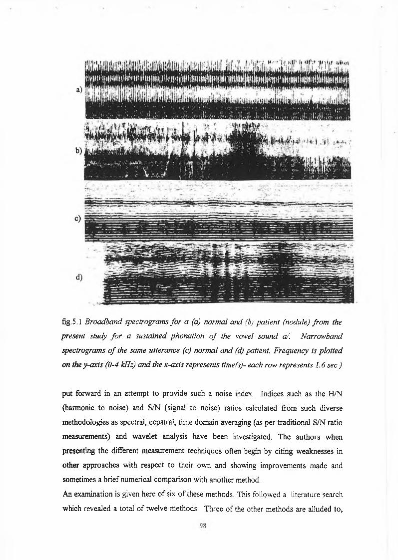
fig.5.1 Broadband spectrograms fo r a (a) normal and (b) patient (nodule) from the

present study fo r a sustained phonation o f the vowel sound cl'. Narrowband

spectrograms o f the same utterance (c) normal and (d) patient. Frequency is plotted

on the y-axis (0-4 kHz) and the x-axis represents time(s)- each row represents 1.6 sec )

put forward in an attempt to provide such a noise index. Indices such as the H/N

(harmonic to noise) and S/N (signal to noise) ratios calculated from such diverse

methodologies as spectral, cepstral, time domain averaging (as per traditional S/N ratio

measurements) and wavelet analysis have been investigated. The authors when

presenting the different measurement techniques often begin by citing weaknesses in

other approaches with respect to their own and showing improvements made and

sometimes a brief numerical comparison with another method.

An examination is given here of six o f these methods. This followed a literature search

which revealed a total of twelve methods. Three of the other methods are alluded to,

although not investigated. The basic idea behind each method is carefully developed

and adjustments (and different interpretations) are given where it has been felt

necessary. The details o f the methods are given in depth in section 5.3 but firstly we

turn our attention to three very important issues associated with determining and

interpreting H/N ratios. The development motivates the need for new measurement

techniques and new analysis ratios.

Firstly, to what extent do presently used indices represent the amount o f ‘noise’

present in a signal as opposed to the presence o f other perturbation measures such as

jitter and shimmer ? This question is carefully addressed and the approaches by which

to overcome the methological issues are clearly stated. The different spectral

consequences are clearly illustrated, hence providing an approach for independent

measurement of jitter, shimmer and additive noise.

The question (often overlooked) as to what is noise is addressed and defined. The H/N

and S/N are clearly explained and the relationship between the H/N (S/N) at the source

is related to the H/N at the output. Defining these relationships leads to a discussion

on what is the most pertinent measurement to make on the acoustic speech waveform.

Several possibilities exist:

1 level o f harmonics

2 level o f noise

3 magnitude o f H/N (S/N)

4 level o f H/N at a given frequency location

5 geometric ratios

6 limiting the frequency range

7. Ratio between various harmonic numbers (or harmonic regions)

A discussion is given on what inferences are to be made from these spectral

measurements with respect to glottal flow and hence the vibratory pattern o f the vocal

cords.

99

5.2 Harmonic Intensity Analysis: Preliminary

Considerations

5.2.1 Definition of Noise

Conspicuously absent from the literature relating to noise levels in pathological voices

is a clear definition o f what is meant by ‘noise’. An operational definition generally

given (or more often implied) is that noise constitutes the non-harmonic energy found

in the speech signal. Thus, a perfectly periodic waveform exhibits an infinite harmonic

to noise ratio: the unperturbed synthesis files used in the present study give harmonic

to noise ratios of 300 dB. Contrary to this, the waveforms from real voices vary to a

certain extent, due to such effects as flutter or tremor and therefore contain ‘noise’

energy with harmonic to noise ratios in the 20 to 30 dB range being typical (depends

on ratio type and methodology). Also, jitter and shimmer artifacts contribute to a

reduction in measured H/N ratios since by this definition they are properly labelled

noise components. Consequently, for an overall measurement o f ‘noise’ according to

the above definition, all perturbation artifacts should be included.

Nonetheless, we are also concerned with characterising the vibratory pattern o f the

vocal folds based on the waveform analysis and in respect o f this, we are required to

differentiate, if possible the different origins of the noise. Four distinct possibilities

exist.

1. Variation o f pitch period (jitter)

2. Variation of peak amplitude from cycle to cycle (shimmer)

3. (Additive) Noise

4. Variation o f waveform within a vibratory cycle

Number 3 refers to the turbulent flow produced at the glottis during phonation,

perhaps due to lack of, or, incomplete closure or due to the presence o f mass lesions.

100

Stevens et al9 have carried out some investigations into the nature o f the turbulent

flow, although further studies relating to vocal pathologies are required. This noise

source is generally modelled as random, mean zero, Gaussian noise. The use o f the

word ‘noise’ here leaves room for ambiguity. However, the context o f the word usage

usually suffices and we generally refer to the noise o f turbulent origin as ‘additive

noise’. The more general usage o f the word ‘noise’ in the vocal pathology literature

implicitly means noise o f some origin, other than 1,2 and 4 above i.e. noise o f turbulent

(or possibly other) origin. Except for the definition outline o f noise given in this

section we also use the word ‘noise’ in the narrow sense o f the meaning.

Finally, ‘noise’, can also occur due to specific changes within the vibratory pattern

from cycle to cycle which are not due to shimmer or jitter but due to a change in the

shape o f the glottal waveform (number 4 above). In order to be able to study this latter

characteristic we need to have precise knowledge about the other three noise elements.

Lastly, it should be pointed out that, in theory at least, that a noise free signal by the

above definition could also show considerable pathology, i.e. the waveshape could be

quite irregular, yet consistent from period to period. Conversely, we can imagine a

situation in which the period markers are fixed for each cycle but the waveform

behaves very erratically between the period markers. Spasmodic dysphonia is an

example o f a waveform containing irregular, unrelated waveshapes o f similar period.

5.2.2 Spectral Consequences of Jitter, Shimmer and Additive Noise:

Many authors1,10,11 have observed that H/N ratios may not simply reflect the amount of

additive noise present in a voice signal or as reported by Muta et al10 “glottal source

perturbations distort the harmonic structure and thus affect both noise measures and

harmonic strength measures.” If our ultimate aim is to categorise or make direct

inferences about specific vibratory or glottal events based on acoustic analysis o f the

output waveform, then it is o f paramount importance to be able to make measurements

o f jitter, shimmer and additive noise that are independent o f each other. The

101

interaction effects o f these three parameters has been studied by Hillenbrand1 who

concluded that there are strong measurement interactions among the three variables

and that “caution should be exercised in interpreting measures of perturbation and

noise in terms of specific aspects o f the laryngeal vibratory cycle”. For example,

adding increasing amounts o f jitter not only affects the pitch perturbation but also

reduces the harmonic to noise ratio o f the signal. Alternatively, adding noise to the

signal causes an increase in the measured jitter and shimmer as well as reducing the

H/N ratio. It is the former problem that we are concerned with here, i.e. the effect of

jitter (and shimmer) on the H/N ratio.

In an attempt to isolate the origin o f the ‘noise’, the spectral consequences o f adding

different amounts o f additive noise, jitter and shimmer are investigated. This is firstly

investigated by referring directly to the Fourier series calculation, from which possible

spectral characterisations of each perturbation measure are postulated. The spectra for

the synthesis files are then examined in order to test the hypotheses.

In applying the Fourier series (eqtn.5.1), two periods o f a perfectly periodic sine wave

with a total time record length, T are considered, as shown in figure 5.2. (In

considering shimmer, the glottal pulse is used in place o f sine waves).

-w a v e fo rm b ( 2 ) -----------b(1)

tim e(s)

fig.5.2 Two periods o f a sine wave with Ti = T2 = T/2. The sine functions for the

firs t two Fourier coefficients are shown (B] and B2 (coincident with waveform)).

102

The basis behind the method is that if each waveform of period, Ti, is exactly the same,

then harmonics will only appear in the spectrum at integer multiples o f (1/Tr=2/T).

However, if the waveforms differ in any respect, then energy appears in the spectrum at

integer multiples o f (1/T). It should be noted therefore, that in this development, odd

harmonics signify some form o f perturbation and even harmonics represent the

unperturbered waveform. Of course, in this case, since the waveform is simply a sine

wave we obtain a single spectral peak at f=l/T i for the unperturbered signal, the

harmonic energy at all other locations being equal to zero.

Ao “ 2 k n t 2 k II tf( t ) = — + 2 (A k C o s(— — ) + B k sin ( - — ))

^ n = 1 A A

eqtn.5.1

2 ^where Ak = — Jf(t)cos(--------)dt eqtn.5.2

T o T

and

2 p 2kntBk = - j f ( t ) s in (— r-)dt

0

t = time

T = periodic time

Ao - mean value of waveform

To see how the Fourier series arrives at this estimate we consider the sine terms o f the

series for each harmonic location kx(l/T) (cosine terms are zero for odd functions).

Fitting the first harmonic, 1/T Hz to the waveform in fig. 5.3 and taking the sum for

the Fourier coefficient, B i(l/T ) we see that (in consideration o f the equation 5.3 and

fig. 5.3) what is obtained in the positive half o f the cycle is also obtained in the negative

half o f the cycle with all contributions to the sum adding to zero. A similar result is

obtained for all higher terms in the series, except for 2x(l/T) when the contributions

add constructively. This is a completely general analysis not specific to sine waves. In

eqtn.5.3

(Fourier Series)

103

„ 2 f . 2 x 2FIt . 2klltBk = —J sm(— - — )sin (-— )dt

0eqtn.5.4

putting k=2, the integrand becomes

2 f , i 2 x 2Ilt 2 p sn tB2 = - j s i n (— —— ) dt = l /2 (l-cos(-^r-)dt

2 2 x 8 x ns m

sin(— ) = 1

and for k * 2, eqtn5.4 becomes

2 f 1Bk — — I —

T ' 2f 2 - k ) x 2 I I t (2 + k )x 2 n t 1

c o s ( --------) — c o s ( ------- =--------) dt

where we have used the trigonometric identity

sinAsinB = ^[cos(A - B) - cos(A + B)]

_2 1 T . (2 - k ) 2n t 1 TT [2 211(2 - k) T ) 2 211(2 + k)

x . ,(2 + k)2IItN )sin( )

eqtn.5.5

eqtn.5.6

eqtn.5.7

eqtn.5.8

0 eqtn.5.9

Therefore showing that our heuristic development is correct i.e. energy is present at the

‘2x l/T ’ harmonic (B2) and zero at all higher harmonics.

104

Now let us consider the case o f shimmer shown in fig.5.3. In utilising the sine wave in

this analysis the result returned is simply a sinewave with amplitude equal to the

average of the sinewave amplitudes as we would expect from the analytical expression.

It is interesting to see the result based on the graphical approach.

-waveform ■b(2)-------- b(1)

ktim e(s)

2/TFourier spectrum

Fig. 5 .3 Two periods o f a sine wave (with Ti = T2 = T/2) with the amplitude o f the

second period reduced to illustrate shimmer. The sine functions fo r the first two

Fourier coefficients are shown (Bj and B2).

Fitting our 1/T1 (2/T) Hz waveform we see that the contributions to B2 (2/T) are

reduced (compare with fig.5.2) i.e. the first even harmonic component is reduced. A ll

higher even harmonics (kx(2/T)) will still sum to zero. Now, considering 1/T, the

contributions are not symmetrical but for the particular case o f the sine wave this

symmetry necessity is removed by the fact that there is a positive and negative

contribution to the energy in each half o f the cycle. All higher odd harmonic energy

contributions sum to zero in similar fashion. The result is a sinusoid of reduced

amplitude. It is interesting to note that the Fourier series (and equivalently, the Fourier

transform) does not differentiate between two sinusoids with amplitudes o f 1, and Vz

respectively, that follow each other as in fig. 5.3 and a sinusoid o f constant

amplitude 3A.

105

For waveforms that are non-symmetrical about the x-axis, energy contributions to

higher harmonics will not cancel in the presence o f shimmer. The glottal pulse model is

examined in fig.5.4. The unperturbered waveform is examined first. Fitting our 1/T1

(2/T) Hz waveform we see that the contributions to B2 (2/T) add constructively, giving

amplitude o f the ‘fundamental’, at the first even harmonic. All higher even harmonics

(kx(2/T)) sum in similar fashion, giving spectral contributions dependent on the

frequency characteristics o f the waveshape - the glottal pulse having a low pass nature

as illustrated in the caption in fig.5.4.

-gR ' b (2 ) --------- b(1)

2/T

Fourier spectrum

Fig.5.4 Two periods o f the Rosenberg glottal pulse (with Tj = T2 = T/2). The sine

functions for the first two Fourier coefficients are shown (B\ and B2).

Now, considering 1/T, the contributions are symmetrical but opposite and sum to

zero. All higher odd harmonic energy contributions sum to zero in similar fashion.

Shimmer is introduced as shown in fig.5.5. The contributions to Bn(2/T) are reduced

due to the decreased amplitude o f the second period o f the waveform. All higher even

harmonics are similarly reduced, and the reduction is in accordance with the spectral

energy contributions for that frequency. The contributions to Bn(l/T ) do not cancel

due to the amplitude difference in the glottal waveform. A similar result occurs for all

higher harmonics and again this is in accordance with the spectral energy contributions

106

Fig.5.5 Two periods o f the Rosenberg glottal pulse (with Ti = T2 = T/2) with the

amplitude o f the second period reduced to illustrate shimmer. The sine functions fo r

the first two Fourier coefficients are shown (Bi and Bi).

for that frequency. Because we cannot shift the waveform to be even or odd, the

cosine terms of the series should also be considered. For the glottal pulse shown in

fig.5.4 the same arguments that were used for the sine terms hold true for the cosine

terms (fig.5.4). Shimmer was introduced with a reduction in the amplitude o f the

waveform in fig. 5.5. This could just as easily have been an increase in amplitude giving

rise to increased even harmonics and in the case of random shimmer we would expect

the overall effect to sum to zero, leaving the amplitude o f the even harmonics

unperturbed. A similar argument can be put forward for the odd harmonic

components. However, since this is a difference measurement we anticipate some

variability, and that the variability increases as the variance o f the shimmer signal

increases.

In the case o f jitter the analysis is somewhat different. In this instance the basis vectors

are separated by 1/T' Hz (fig.5.6). As the two periods are not equal, a contribution

exists at 1/T' Hz. Notice also that there is a reduction in the amplitude contributions at

2xl/T' Hz as the basis vectors no longer match the “fundamental frequency”, 1/Ti.

The situation is analogous to ‘leakage’ that occurs when a non-integer number o f

periods are present in the analysis frame12. This can also be viewed analytically by

107

-w ave fo rm b (2 ) ---------b(1)

1/T2/T'

Fourier spectrum

Fig. 5.6 Two periods o f a sine wave (with Tt * T2 * T/2) illustrating jitter. The sine

functions fo r the first two Fourier coefficients are shown (B/ and B2).

substituting the sine waves o f frequency 1/T! and l/T 2into eqtn.5 .3 and noting that the

calculation of the higher harmonic terms for Bn no longer integrate to zero. Hillenbrand

observed that jitter leads to a more prominent smearing of the harmonic structure at

higher frequencies. We see here that by virtue of the fact that the periods in question

are not sub-multiples o f the basis vectors, higher harmonics appear in the spectrum and

in respect to the sine wave all o f these are noise components. As the even harmonics

(2k) increase, collecting estimates at even multiples o f (1/T'), the difference to the

actual harmonic locations o f 2kxl/Ti and 2kxl/T 2 increases, therefore reducing the

contributions to higher even harmonics (1/T') as the frequency increases. However, at

some upper frequency location we expect the even analysis harmonic 2kx(l/T') to

match or cross over the signal harmonic, 2kx(l/Ti), therefore producing the reverse

effect with 2kx(l/T i) gaining more o f the energy contributions and 2kx(l/T 2) obtaining

less. The same process is simultaneously occurring for kx(l/T 2). Harmonic

reinforcement will also occur when kx(l/T i-l/T 2) matches either o f the signal

frequencies 1/Ti or I/T2. Superimposed on this harmonic interplay between the analysis

basis vectors and the signal frequencies, as the harmonic number increases, due to the

frequency characteristics o f the signal, the energy at higher harmonics decreases.

Therefore the contributions at between harmonic locations are dependent on the jitter

108

artifact and signal characteristics with the signal harmonics (1/Ti and 1/T2) becoming

further separated at the upper partials with occasional reinforcement occurring when

k x ( - ^ - ^ ) = m x \ r m x H eqtn.5.10I 1 1 2 1 1 1 2

The odd analysis harmonics ((2k + l)x l/T ) also receive reinforcement at particular

frequencies governed by

k x ( 7 r r " 7 ) = m x 7 eqtn.5.111 1 + 12 11 l l

Eqtn.5.11 can similarly be written for (1/T2). Because the frequency differences in

equation 5.11 may be large it may be more convenient to simply match the 1/(Ti+T2)

to the integer number on the right side of the equation. Also, equations for minima can

be written by adding Vi to ‘m’ in the above equations. Note that in a two cycle analysis

development it is impossible to differentiate cyclic and random jitter. In the case of

cyclic jitter, the above mentioned ‘odd analysis harmonic’ is equivalent to the

subharmonic frequency and the development is exactly as laid out above. For random

jitter, the above mentioned trends are still valid but the random variability introduced

will have a large bearing on the overall spectral characteristics.

Considering the addition o f mean zero random noise (fig. 5.7), it can be seen that the

basis vectors are correct but that the spectral estimates at even harmonics are more

variable and energy appears at odd harmonic locations due to the random noise

components. If the variance o f the noise increases we would expect the variance o f

our spectral estimates to increase also. The sine wave signal plus noise may be

represented by the following equation,

2 x 2ITts(t) = sin(— - — ) + q(t) eqtn.5.12

where q(t) is the noise component

109

We have seen (eqtn5.4 to eqtn.5.9) that the Fourier series for the sine wave gives zero

energy at all frequency locations except 2x 1/T. Therefore for n ^ 2 we have

2 r , s in2nkn t ,Bk = — Jq( t ) dt eqtn.5.13

o

Since q(t) is random it can be inferred that it provides energy contributions to all

harmonics in the spectrum. In fact for truly random noise the integral in eqtn.5.11

cannot be evaluated and the autocorrelation of q(t) must be evaluated prior to

integration13. Fourier estimates o f noise are dealt with in more detail in section 5.3.4.

Our development, simply through a direct implementation o f the Fourier series and a

brief reference to the Fourier transform has led to the above spectral characterisations

of shimmer, jitter and additive noise respectively.

Fig. 5.7 Two periods o f a sine wave (with TI = T2 = T/2) in the presence o f additive

noise. The sine functions fo r the first two Fourier coefficients are shown (BI and B2).

In summary, for shimmer signals the level of the even harmonics is unchanged and the

level of odd harmonics increases with the variance o f the shimmer and the contributions

to the noise at a given frequency are in direct relation to the contributions to the signal

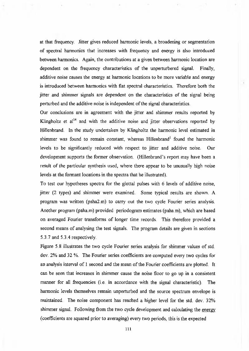
at that frequency. Jitter gives reduced harmonic levels, a broadening or segmentation

o f spectral harmonics that increases with frequency and energy is also introduced

between harmonics. Again, the contributions at a given between harmonic location are

dependent on the frequency characteristics o f the unperturbered signal. Finally,

additive noise causes the energy at harmonic locations to be more variable and energy

is introduced between harmonics with flat spectral characteristics. Therefore both the

jitter and shimmer signals are dependent on the characteristics of the signal being

perturbed and the additive noise is independent of the signal characteristics.

Our conclusions are in agreement with the jitter and shimmer results reported by

Klingholtz et al14 and with the additive noise and jitter observations reported by

Hillenbrand. In the study undertaken by Klingholtz the harmonic level estimated in

shimmer was found to remain constant, whereas Hillenbrand1 found the harmonic

levels to be significantly reduced with respect to jitter and additive noise. Our

development supports the former observation. (Hillenbrand’s report may have been a

result o f the particular synthesis used, where there appear to be unusually high noise

levels at the formant locations in the spectra that he illustrated).

To test our hypotheses spectra for the glottal pulses with 6 levels o f additive noise,

jitter (2 types) and shimmer were examined. Some typical results are shown. A

program was written (psha2.m) to carry out the two cycle Fourier series analysis.

Another program (paha.m) provided periodogram estimates (paha.m), which are based

on averaged Fourier transforms o f longer time records. This therefore provided a

second means o f analysing the test signals. The program details are given in sections

5.3.7 and 5.3.4 respectively.

Figure 5.8 illustrates the two cycle Fourier series analysis for shimmer values o f std.

dev. 2% and 32 %. The Fourier series coefficients are computed every two cycles for

an analysis interval o f 1 second and the mean o f the Fourier coefficients are plotted. It

can be seen that increases in shimmer cause the noise floor to go up in a consistent

manner for all frequencies (i.e. in accordance with the signal characteristic). The

harmonic levels themselves remain unperturbed and the source spectrum envelope is

maintained. The noise component has reached a higher level for the std. dev. 32%

shimmer signal. Following from the two cycle development and calculating the energy

(coefficients are squared prior to averaging) every two periods, this is the expected

i l l

fneq. (Hz) (a)

10o

m2 . -20

Q. -30E« -40

-50

-60freq. (Hz)

(b)

fig. 5.8 Two cycle Fourier series coefficients fo r glottal pulse signals with (a) 2% std.

dev. random shimmer and (b) 32% std. dev. random shimmer

result, with the harmonic levels on the average remaining unperturbed and energy

introduced between harmonics which increases with increasing shimmer. In

considering the periodogram estimate (Fourier amplitude is gathered over many cycles

before calculating the energy) o f the same signal (fig.5.8(b)), we again expect the

harmonic variation to sum to zero as shown. A similar consideration of the between

harmonics might lead one to conclude that a summing to zero also occurs here since

the shimmer signal has a mean o f zero. However, the periodogram graphs show

exactly the same trend as the two cycle analysis plots. The periodogram plots are an

average of six 4096 point spectra hopped 1024 points. This averaging has reduced the

variance of the spectral estimates (section5.3.). Figure 5.10 shows the variance

associated with a single Fourier transform spectrum o f 4096 points for the signals with

std. dev. 2% and 32% shimmer. The increased variance of the between harmonic

112

ampi

. (d

B)

0 500 1000 1500 2000 2500 3000 3500 4000 4500 5000

Frequency (Hz)(a)

fig.5.9 (a) Periodogram estimate or power spectral density (PPx2dB,PPx32dB) fo r the test shimmer signals ofstd. dev. 2% and 32 % .

113

*fs2-fs32

freq.(Hz)(b)

Fig. 5 .9 (b) Fourier transform estimates (fs2 and fs32) o f the same signals illustrating

the increased variance o f the std. dev. 32% signal’s between harmonic energy.

estimates is now very obvious. Therefore as the transform gathers it’s frequency

estimates the variance o f the estimates increases according as the shimmer signal

increases. This variance is still symmetrical about zero, however the square o f the

variance is not, therefore raising the noise level as shown. The variance is also present

at harmonic peak locations but due to the fact that the signal is much larger than the

variance the effect is very small when the squaring operation is applied in order to

obtain the energy. Note the variance in question here is linearly related to the source

variance but that it is o f smaller magnitude.

For cyclic jitter (fig.5.10 (a)) we see that the main characteristic is that a strong

subharmonic has been introduced at an octave lower than fO, as might have been

expected. The amplitude in the subharmonic spectrum can be seen to follow an

interesting trend, which is governed by eqtn.5.11. Substituting values gives matches

the 23rd ‘106 Hz signal component’ with the 50th (signal-subharmonic). This also

occurs for the ‘ 109.9 Hz signal component’ at about this frequency.

For random jitter (fig5.10 (b)) the spectrum is somewhat different. The harmonic

structure is severely affected for the std. dev. 6% random jitter signal shown in the two

cycle Fourier series spectrum. The spectral envelope is maintained, however, with

114

0 1000 2000 3000 4000 5000

frequency (Hz)

fig. 5.10 (a) Periodogram estimate fo r 3 % cyclic jitter o f source signal (b) Two cycle

Fourier Series averaged energy spectrum for random jitter signal with 6% std. dev.

noise energy i.e. non harmonic energy, becoming nearer in magnitude to the harmonic

energy as the frequency increases.

The periodogram provides further information. For a perfectly periodic signal the

estimate at a given frequency location is the convolution o f the Fourier transform o f the

window function with the Fourier transform o f the signal at that frequency. This is

shown in fig. 5 .11 for the 110 Hz glottal waveform with a random jitter component of

std. dev. 6%. As the frequency increases the spread o f the signal about the higher

harmonics increases, reducing the amplitude at kxl 10 Hz locations. Cross over effects

115

ffl -40

H -42| - -44 « -46

—1— 2100

----------

2700— I------------------ 1—2300 2500 2900

fig.5.11 Periodogram estimates o f the random jitter signal (a) 0-900Hz showing

spectral broadening and harmonic decomposition, (b) in general harmonic structure

is diminished with a reappearance in harmonic structure at ~1500Hz (c) as fo r (b)

with harmonic reappearance ~2650 Hz

116

also occur. Hence there is a broadening o f the spectral peak due to the window

function. For the higher harmonics the difference between the two frequency

contributions increases causing further broadening o f the spectral peaks. However if

the jitter is large the contributions may become individually resolved as the harmonic

number increases giving rise to a more irregular looking spectrum. However, some

reappearance of harmonic structure is also evidenced due to the cross over in jittered

frequencies as mentioned earlier (5.11(b)) (5.11(c)).

Figure 5.12 shows the effect o f adding random Gaussian noise to the glottal source.

The level o f the harmonics themselves are unaffected except as the noise floor moves

upwards, in a sense consuming the lower level harmonics as it moves. The noise

spectrum is white as expected. The periodogram reveals no extra information (not

shown).

fig.5.12 Two cycle Fourier Series averaged energy spectrum fo r random additive

noise o f s td dev. 2 %.

So, considering the four cases o f cyclic and random jitter, shimmer and additive noise

we see that there are clear spectral differences. With this in mind it may therefore be

possible to develop quantitative spectral measures that differentiate the four types. For

example, a constant value o f H/N(o) for all © would indicate shimmer. A first

examination o f the random jitter and additive noise graphs indicates that they are

somewhat similar with early harmonic structure still present and higher harmonics

completely missing.

117

ACOUSTIC

INDEX

/PERTURBATION

TYPE

HARMONIC

LEVEL

(H)

NOISE LEVEL

(N)

HARMONIC

TO NOISE RATIO

(H/N)

Shimmer Constant Increases in direct

proportion to signal

characteristics at

that frequency.

Constant for all

frequencies

Random Jitter Reduced Increases-signal

dependent.

Amplitude of noise

is greater at lower

frequencies.

Reduced.

Decreases with

increasing

frequency.

Cyclic Jitter Variable

dependent on

individual pitch

periods

Increased- a

subharmonic regime

is introduced.

Reduced-dependent

on pitch period

relationship

Random Additive

Noise

More variable Increased

independent of

signal

Reduced- decreases

with increasing

frequency

Table5.1 S u m m a r y o f S p e c t r a l C h a r a c t e r i s t i c s o f S h im m e r , R a n d o m J i t t e r , C y c l i c

J i t t e r a n d A d d i t i v e N o i s e

However, closer examination reveals that the noise level in the additive noise case is

considerably higher and therefore a measurement o f H/N ratio from 1 to 4 kHz

indicates a perturbation o f either additive noise or jitter but a subsequent measurement

o f the noise level will reveal which o f the two is actually present. The subharmonic

regime o f the cyclic jitter spectra suggest a method for quantifying this type of

perturbation. A summary o f the spectral characteristics o f the four perturbation

118

measures are given in Table5.1. To surmise, we have hypothesised what the spectral

characteristics o f jitter, shimmer and additive noise are and then produced spectra from

the synthesized data in order to examine our hypotheses, which were found to be in

good agreement. Therefore, what is now required is some definite spectral

measurements to objectively prove the above assumptions in a quantitative manner.

Section 5.3 provides a detailed description o f the quantitative analysis techniques that

have been developed in order to make these spectral calculations.

5.2.3 Harmonic to Noise Ratio of the Glottal Source and it’s Relation to

the Harmonic to Noise Ratio of the Output Radiated Speech Waveform

In acoustic analysis o f tape recorded speech, the acoustic speech waveform is a

complex signal consisting o f the source excitation convolved with the vocal tract filter

function, followed by radiation at the lips. The objective is to take measurements from

this output signal and make inferences regarding the source signal and hence the

underlying vibratory mechanism.

From the source/filter model o f speech production we have that

s(t) = e(t)* v(t) eqtn. 5.14

s(t) = (e(t)+ n(t))* v(t) eqtn. 5.15

S(co) = [E(co) + N(co)] x V(co) = E(cg) x V(co) + N(co) x V(<a) eqtn. 5.16

s(t), S(w) = output waveform and Fourier transform

e(t), E(q) = source signal and Fourier transform

n(t), N (o) = additive noise and Fourier transform

v(t), V(co) = impulse and frequency response o f the vocal tract

where * indicates convolution.

119

As discussed in section 5.1 the harmonic to noise ratio (H/N) taken from the output

speech waveform or spectrum is a commonly used measure in assessing vocal

pathology. It is pertinent to ask, in what sense is the harmonic to noise ratio o f the

speech waveform indicative o f the harmonic to noise ratio o f the source signal.

Rearranging 5.7 gives

H x E(co)xV(co)— (<a) = ------------------ eqtn.5.17N 1 N(co) x V (o ) 4

which is the H/N ratio at frequency ‘oo’. Within the limits o f the source filter model, the

H/N ratio at a given frequency location is the same for source and filtered waveform.

Therefore we can write

H H— (co)(waveform) = — (ra)(source) eqtn.5.18N N

However, the harmonic to noise ratio is usually determined over the complete

frequency range or over a band limited region but not at discrete frequencies.

Therefore eqtn.5.15 is summed in order to obtain the overall harmonic to noise ratio.

The ratio is generally expressed in dBs.

JJ— (waveform) = 1 0 x loglO

£ E (c o )V (0 )CO__________

Z N ( 0 )V (o )eqtn.5.19

A consideration o f this case shows

H H— (waveform)*— (source) eqtn.5.20N N

eqtn.5.19 is a generic formulation o f the harmonic to noise ratio as calculated by

various investigators. Variations include inverting the ratio, giving the noise to signal

120

ratio or giving the signal to noise ratio by including the noise and harmonics as signal.

Bandlimiting the range over which the ratio has been calculated has also been

investigated. Despite the fact that several variations o f eqtn.5.17 that have been

implemented, no study has attempted to relate the S/N (out) to the S/N (source). A

simple numerical example will help illustrate the problem of simply using eqtn.5.17 to

make inferences regarding source characteristics.

Example

As a simple illustration of eqtn.5.17 we take two frequency values, one low ( c o l ) and

one high ( c c > h ) and consider some numerical values.

E (col) = 1 0 0 0 , E(coh) = 10

N(cc>l) = N(coh) = 1

H ( o l ) = 10

H (o h ) = 100

H 1000+10 1010— (source) = -------------= ------ = 505 = 27dBN ' 1+1 2

H x 1000x10+10x100 10100— (output)= ------------------------- = -------- = 20dBN H ' 10+100 110

Therefore, H/N (source) ^ HZN(output) and the high frequency component has gone

from having very little effect to dominating the ratio.

Taking an alternative approach allows us to recover the H/N ratio o f the source.

H 1 ^ E(w)H(w)— (source) = - ¿ . 7 ~ ~ " eqtn.5.21N M “ N(w)H(w)

This ratio, which we indicate by H/Ns, reflects the H/N ratio o f the source in a true

sense only when the noise is equal for all frequencies. This is so for truly mean zero,

121

Gaussian noise. But the ratio can be o f use even when this is not the case. As stated in

the introduction, a prime objective is to make measurements that will correlate with

based measures. Other researchers have made similar remarks:

“We also need to consider the purpose of our objective analyses. One analytic goal may be to determine the conditions of the vocal folds in order to study the pathophysiological mechanisms of voice disorders. In this case acoustic characteristics irrelevant to perception may be important. If the goal of the analysis is to predict the perception of the voice quality, then we have to consider features of our hearing mechanisms such as masking, frequency sensitivity, and so on.” (Gauffin et

It can be seen that 5.18 attempts to match physical attributes, in order to obtain

information regarding the glottal source. In addressing perceptual correlations, a ratio

which we have termed the geometric dB mean (eqtn.5.19) has been developed.

The term geometric mean comes form the fact that the additions involve logarithms

higher frequency components in a crude manner at matching the frequency analysis

processes o f the ear. Extracting the ratio from the dB signal probably gives too much

vocal quality assessment. To date, these ratios have not been applied to the

investigation o f pathological voice types.

5.2.4 Harmonic Intensity Level

The preceding section examined the harmonic to noise ratio and suggested variations

that may be o f use in studying both source and perceptual characteristics. Previous to

this, section 5.2 outlined possible causes o f ‘noise’ found in pathological voice types.

either the physical underlying processes o f vocal fold vibration or with perceptual

eqtn.5. 2 2

and is therefore somewhat equivalent to taking the product o f the linear values and

taking the M* root i.e. the geometric mean. This effectively gives greater weight to the

weight to the higher frequency components1 6 and perceptually based frequency

weighted ratios17, having similar form to the above ratio, have been developed for

122

Therefore, we have examined the ratio itself and the denominator but have somewhat

neglected the numerator i.e. the energy at harmonic locations. The harmonic energy is

perhaps the most important o f the three. Recent developments have tried to develop a

frequency domain parameter set relating to the LF model o f glottal flow (fig.5.13)

developed by Fant and co-workers18. The level of the harmonics is o f prime

importance in these developments. Often, in spectral analysis, the level o f the

harmonics is often overlooked, possibly because the spectrum is usually given in dB

and relative values are often o f more immediate interest. In it’s most basic form, the

level o f harmonics provides an additional parameter for investigating the waveform.

However, taking particular ratios between specific harmonics provides a means of

assessing different flow characteristics and hence information can be obtained

regarding the vocal fold vibrations.

fig.5.13 L F m o d e l

o f g l o t t a l f l o w .

T h e t o p tw o r o w s :

L F - f l o w U g( t) , f l o w

d e r i v a t i v e U g '(t),

a n d s p e c t r u m o f

U g " ( t) a t v a r y i n g

E / E » c o n s t a n t U 0 ,

a n d T a = 0. I n th e

>.a o.4 o.6 os b o t t o m r o w : L F

f l o w a n d s p e c t r u m

U g "(t) w h e n

m a i n t a i n i n g

c o n s t a n t E e ( T a= 0) .

123

The four parameters of the model are Rk, Rg, Ra and Ee, which are related to the three

basic time events: (1) the location of the flow peak Tp; (2) the discontinuity point T0 at

glottal closure and (3) the duration of the return phase Ta. Varying the model

parameters produces changes in the frequency spectra as shown in fig.5.13 and an

equivalent frequency domain parameter set has been derived. One important advantage

of a frequency domain parameter set of glottal flow is that it can be used in conjunction

with tape recorded speech (the time domain model requires accurate determination of

low frequency phase). The use of such a frequency domain based glottal flow

parameter set should be of considerable use for investigating vocal pathologies.

However, we have seen in the previous section how the perturbation measures of

shimmer, jitter and additive noise disrupt the harmonic structure in the spectrum and

therefore destroying the possibility of applying the above mentioned frequency domain

parameter set. In the next section techniques are developed in order to overcome these

problems.

5 . 3 A n a l y s i s T e c h n i q u e s :

Following, is an account of nine techniques (Table5.2) which have been developed in

order to provide some form of harmonic to noise ratio for investigating pathological

voices. In presenting the techniques, any deviations from their original design are

clearly stated and the reasons for the changes are detailed explicitly. The order is

given, insofar as possible, to facilitate a continuity of ideas as opposed to listing the

methods in chronological order. In this way we can begin to appreciate the difficulties

that are encountered in obtaining the harmonic to noise ratio. The development leads

to three novel approaches, one of which addresses the problems mentioned in 5.2.

regarding the separability of jitter, shimmer and additive noise. All of the programs

were coded in the Matlab programming language. This section deals expressly with the

methodology and a full description of the results is given in the section 5.4.

124

ANALYSIS

TECHNIQUE

(PROGRAM NAME)

DESCRIPTION ANALYSIS

LENGTH

(SHORTEST UNIT)

kitnos3.m noise reducing

filter 205ms

harmony4.m Spectrum

Analysis

205ms

harmper2.m* Periodogram

Analysis

205ms

noise6.m Spectral Analysis seven periods

harm4.m Spectral Analysis four periods

kojnos3 .m Fourier

Analysis

three periods

psha2.m* Fourier Analysis two periods

harmymn.m Time Domain one period

pshal .m* Fourier Analysis one period

Table. 5.2 L i s t o f n i n e a n a l y s i s t e c h n i q u e s i m p l e m e n t e d i n t h e p r e s e n t s t u d y

w h e r e * i n d i c a t e s a n o v e l p r o c e d u r e . S o u r c e c o d e i s g i v e n i n a p p e n d i x A .

125

As stated by Kitajima "the basic idea is to pass the voice through a noise reducing filter

at first, and then compare the pre- and post- filtered voices in their effective values". A

stable portion of the vowel a/ is taken, sampled at 5 kHz (cut off frequency 2.5 kHz)

for 205 ms and padded up 4096 samples. The approach is to obtain the power

spectrum of the signal, apply a moving average filter to this harmonic spectrum and

count as signal the components above the moving average estimate, and as noise those

components below the moving average filter. This situation is depicted in fig.5.14 and

given in equation form as

|E(f)|2 = |z(f)|2 > |z(f)|2 - S(f) i f lz (f)|2>S(f)eqtn.5.19

|E(£)|2 = 0 if |Z(f)piS(f)

|E(f)|2 = |Z(f)|2 - [S(f)+C(f)] if |Z(f)|2 > S(f) + C(f) eqtn 5 20

where is Z(f) is the spectrum of the original signal

S(f)=moving averaged spectrum

E(f)= noise reduced spectrum

C(f) = standard deviation of S(f)

A noise reducing filter is then developed based on 5.19 and 5.20. The filter is given as

H(f) =E(f)/Z(f) eqtn. 5.21

Z(f) is already known and E(f) is obtained as above and therefore H(f) could be

calculated for each subject. A voice signal is then passed through the filter H(f) and

the filtered voice was designated as Y(f). This is shown schematically in fig.5.15. The

5.3.1 Noise Reducing Filter - Kitajima19

126

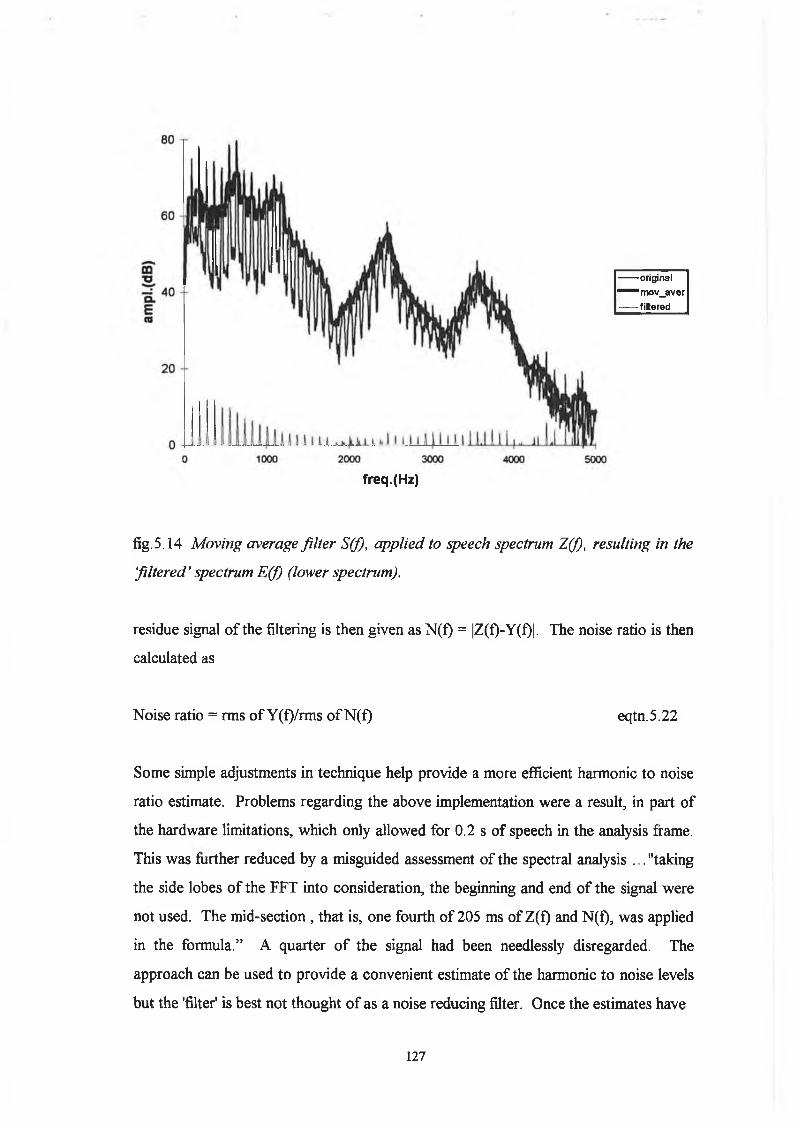
freq.(Hz)

original^ “ "mov_aver filtered

fig.5.14 M o v i n g a v e r a g e f i l t e r S ( f ) , a p p l i e d t o s p e e c h s p e c t r u m 2 ( f ) , r e s u l t i n g i n th e

‘f i l t e r e d ’ s p e c t r u m E ( f ) ( l o w e r s p e c t r u m ) .

residue signal of the filtering is then given as N(f) = |Z(f)-Y(f)|. The noise ratio is then

calculated as

Noise ratio = rms of Y(f)/rms of N(f) eqtn.5.22

Some simple adjustments in technique help provide a more efficient harmonic to noise

ratio estimate. Problems regarding the above implementation were a result, in part of

the hardware limitations, which only allowed for 0.2 s of speech in the analysis frame.

This was further reduced by a misguided assessment of the spectral analysis ... "taking

the side lobes of the FFT into consideration, the beginning and end of the signal were

not used. The mid-section , that is, one fourth of 205 ms of Z(f) and N(f), was applied

in the formula.” A quarter of the signal had been needlessly disregarded. The

approach can be used to provide a convenient estimate of the harmonic to noise levels

but the 'filter' is best not thought of as a noise reducing filter. Once the estimates have

127

Voice Signal

Low pass filter (cut-off 2.5kHz)

A/D convertion, n=1024, level +/-2048

FFT

Voice Signal

Low pass filter (cut-off 3800 Hz)

A/D convertion, n=2048,

level +/-8192

FFTS(f)

Z(f)

Noise Reduction moving average

filter Z(f)

IFFT

Y(f)Y(f) (also in dB)

(result)

N(f) = Z(f) - Y(f)

Noise Ratio = rms of Y(f)/rms of N(f)

(a)

Noise Ratio =

rms of Y(f)/rms of N(f)

(optional)

(b)

fig. 5.15 (a) S c h e m a t i c d i a g r a m o f a n a l y s i s s t e p s i n v o l v e d f o r t h e n o i s e r e d u c i n g f i l t e r

a s i m p l e m e n t e d b y K i t a j i m a a n d (b) a s i m p l e m e n t e d i n t h e p r e s e n t s t u d y

been taken from the spectrum (fig.5.14), the harmonic to noise ratio can be directly

inferred. Therefore, subsequently developing a filter based on these measurements is

probably not necessary. The filter gives no extra information regarding the signal or

noise being obtained. Another simple, but important modification is to average ‘n7

spectral samples for the moving average filter, where ‘n’ is dependent on the pitch

period and not static (41 points).

Referring to the schematic diagram of the method as implemented by Kitajima, the

many extra steps that were necessary for the filtering, involving a forward and inverse

FFT can be seen. The filtering simply provides a noise estimate via a multiplicative

128

process based on the noise estimate that was originally obtained through an additive

process. The method implemented here (fig.5.15(b)), simply applied a moving average

(dependent on the pitch period) filter to the spectrum. Then the resulting signal plus

it's standard deviation were subtracted from the original spectrum to obtain the noise

reduced signal. Two separate estimates were taken, one based on the linear spectrum

(kitnos3.m) and the other was obtained from calculations taken directly from the dB

spectrum (kitnosdB.m). The process of calculation is best illustrated by referring to

fig.5.14. In the case of the dB spectrum the average is calculated from the spectrum in

dBs, giving what might be termed a geometric mean of the amplitudes. The linear ratio

returned form ‘kitnos3.m’ is calculated as shown in eqtn.5.22 and then converted to dB

which is the more usual form and hence more useful for comparison purposes. Also,

10kHz sampling was used in this study, and frequencies up to 3.8 kHz were analysed.

205.3.3 Relative Harmonic Intensity - Hiraoka et al

The relative harmonic intensity (Hr) is a direct measurement taken from the Fourier

magnitude spectrum in linear scale and is given by

f

Z p1H. = i> 2 x 100(%) eqtn.5.23

The vowel aJ was used for analysis, sampled at 20 kHz. A 4096 point FFT was taken,

corresponding to approximately a 0.2 second segment of speech at this sampling

frequency. In order to match this condition with 10 kHz sampling, 0.2 second of the

speech sample was extracted for analysis and padded out to 4096 points for Fourier

transform analysis. The method given20 for locating fO was originally used, though it

was found preferable to use any accurate fO extraction method to locate the

fundamental peak and then find the subsequent harmonic locations by searching for

peaks in the region of nxfO±ml, where ‘ml’ represents the main lobe width of the

analysis window. Surprisingly, the method used for calculating the amplitude of the i*

129

freq.(Hz)

fig.5.16 S e c t i o n o f 4 0 9 6 p o i n t F F T p o w e r s p e c t r u m o f 2 . 0 4 8 m s o f s p e e c h g i v i n g a

m a i n l o b e w i d t h o f 8 x p a d 2 / M = 8 x 4 Q 9 6 / 2 / 2 0 4 8 = 8 p o i n t s .

harmonic is not given although it is implicit that the peak amplitude at the harmonic

location was taken from the linear spectrum. In this implementation, the total energy

of the main lobe was taken as the energy for the i* harmonic and taking the sum for all

harmonics gave total harmonic intensity. The main lobe width21 (fig.5.16) for the

Hamming window used is given by ‘8xpad/2/M’ where pad is the FFT length and M is

the sample length taken. Several other noise indices were taken from the spectrum to

give a total of ten different measures reflecting S/N, H/N, Hr, Sr and HNgeo and

different regions of the spectrum were investigated.

5.3.3 Periodogram Averaged Harmonic Analysis (PAHA)

In considering the estimation of noise levels in pathological voices we have generally

referred to the noise as being an additive random component. In that sense we are

making an a priori assumption that there exists an underlying deterministic process

which has been obscured or contaminated through the addition of random noise.

However, we can also view the system under investigation to be the result of a

stochastic process giving rise to a stationary random signal and based on this

viewpoint make inferences about the underlying structure, if any, through the

130

application of statistical analysis tools. Such an analysis tool is the periodogram

estimate or power spectral density function. It has been shown, however, that the

periodogram does not provide a consistent estimate as the window length increases and

that the variance of the estimate is of the same size as the power spectrum estimate

under investigation22 (Consider for comparison, the mean of a stationary random

process which approaches the true mean as the window length increases). However,

the variance can be reduced if we make several consecutive estimates of the signal i.e.

N estimates reduces the variance by 1/N. Welsh23 has shown that overlapping by 2:1

and hence increasing the number of estimates by a factor of two reduces the variance

further, by almost a factor of two also. In terms of the power spectrum, the expected

value of the average periodogram estimate is the convolution of the true power

spectrum with the Fourier transform of the autocorrelation of the window function21.

The spectral consequence of the autocorrelation is to double the mainlobe width22

(fig.5.16). For a rectangular window this gives

C w wL - H M

0 ’ 0the[W1Se eqtn.5.24

^ f sin(<22i , / 2 ) YO h’w ~ I ;

V sin(iy/2)y eqtn.5.25

P x x = ---------------f F x x ( 0 ) C ™ ( e ; W )eqtn.5.26

where c « is the autocorrelation of the rectangular window

Cww is the Fourier transform of Cw

Pxx is the power spectral density or periodogram estimate

131

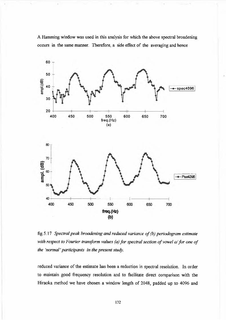
A Hamming window was used in this analysis for which the above spectral broadening

occurs in the same manner. Therefore, a side effect of the averaging and hence

-spec4096

freq.(Hz)(a)

-PXX4096

freq.(Hz)(b)

fig. 5.17 S p e c t r a l p e a k b r o a d e n i n g a n d r e d u c e d v a r i a n c e o f ( b ) p e r i o d o g r a m e s t i m a t e

w i t h r e s p e c t t o F o u r i e r t r a n s f o r m v a l u e s ( a ) f o r s p e c t r a l s e c t i o n o f v o w e l a / f o r o n e o f

t h e ‘n o r m a l ’p a r t i c i p a n t s i n t h e p r e s e n t s tu d y .

reduced variance of the estimate has been a reduction in spectral resolution. In order

to maintain good frequency resolution and to facilitate direct comparison with the

Hiraoka method we have chosen a window length of 2048, padded up to 4096 and

132

- - - H/NS — — source spectrum

hopped by 1024 points providing 8 independent spectral estimates for about 1.2

seconds of speech. The harmonic estimates were obtained as per the Hiraoka method

_ -10 mT3tT -20 E« -30

-40

-50

fig.5.18 C o m p a r i s o n b e t w e e n o r i g i n a l s o u r c e s p e c t r u m ( g l l 0 a r 4 ) f o r 1 1 0 H z f i l e w i t h

s td . d e v . 4 % a d d i t i v e n o i s e a n d t h e H / N s(co) d e r i v e d s o u r c e s p e c t r a l r a t i o c a l c u l a t e d

f r o m t h e o u t p u t r a d i a t e d w a v e f o r m .

but with double the mainlobe width and all of the above mentioned ratios were also

calculated. In addition to these ten ratios, the H/Ns ratio (section 5.2.) was also

estimated, using various harmonic numbers which provided a further six indices. The

spectra obtained as a result of the H/Ns(co) procedure are shown in figure 5.17. These

spectra bare a close resemblance to the source spectra as shown in fig. 5.18. It is

interesting to consider this derivation in terms of the frequency response of our linear

time invariant system to a white noise input.

S y y ( e jiB ) = C ( e jffl )Sxx(eJiB ) eqtn.5.27

Syy(eJ" ) = C ( e J- ) o * 2 eqtn.5.28

where is the power spectrum of white noise and C(ei<0) is the system function.

ox2 is the variance of the noise signal and Syy is the output of the system.

133

5.3.4 Normalised Noise Energy - Kasuya et al23.

The normalised noise energy (NNE) is the only method to include phase in the noise

calculation, or rather to have taken phase into consideration. In the vast majority of

speech processing applications phase is not considered and can be quite difficult to

calculate and ironically is very sensitive to noise. Secondly, the ear is not responsive to

phase information from the speech signal. In any case when considering random

processes, the random signal is by definition considered to have random phase.

The speech signal in the mth frame is given by

X m ( n ) = Sm(n) + W m ( n ) , n = 0 , 1 , . . . , M - 1 eqtn.5.29

taking Fourier transformation

X m(k) = S m ( k ) + W m ( k ) , k = 0 , 1 , . . . , M - 1 eqtn.5.30

Then the NNE is defined as

N N E = l O l o g

1 NH Lf E X | w ( k ) | ’

k = N Lm = 1eqtn.5.31

k = N lhi =1

where xm(n) = m“ 1 frame of vowel phonation

with periodic component s,„(n) and additive noise

component wm(n)

M is the number of samples within the frame

NL=[N fLT], NH = [NfHT]

where L is the number o f frames and fL and fH determine the highest and

lowest frequencies

134

The denominator in equation 5.31 is calculated directly from the DFT estimate and

therefore the problem is to devise a method o f estimating the numerator or noise.

Representing the squared magnitude o f the DFT o f the signal plus noise gives

|X m ( k ) | = |S m ( k ) |2 + |w m (k ) | 2

+ 2 |S m( k) | |w m ( k ) | c o s [ 0 ( k ) - 0 ( k ) ] , k = 0 , 1 M - 1 eqtn.5.32

Since the signal becomes small in the harmonic dip region (fig.5.19) the noise can be

estimated directly from the spectrum as

| w „ ( k ) | ! = | Y. |X™(r) | 2 ( N , ) - ' + X ¡X m(r)j2 ( N i - i ) -1 1 , k e P,I r e D i r e D i + 1 J

eqtn.5.33

An interpolation o f estimates from adjacent dip regions is used in the estimation of

noise in the peak region. Therefore the phase has been considered, yet not calculated.

From the development o f the spectral consequences o f various perturbations outlined

in section 5.2, it has been observed that the harmonic energy remains quite stable in

some instances (shimmer) and reduces in others (jitter). Taking this into consideration,

perhaps it is not appropriate to estimate the noise in the peak regions in this manner.

We have seen that the noise floor moves up rather than that harmonic energy reduces

in the perturbation o f shimmer and additive noise. The main problem with this estimate

of noise in the peak region is that here the magnitude will always add, therefore

implying that the noise actually adds to the signal strength. If the phase had been

included the signal would on average contribute zero energy to the peak region, simply

adding more variability to the estimate which is consistent with our development

above. Therefore in the absent o f phase information it is not applicable to estimate the

noise in the harmonic region in this manner and this type o f approach is more suited to

noise considerations where the noise is a competing sinusoid or other well determined

signal. The final result in the analysis is simply a doubling o f the noise component of

135

freq.(Hz)

fig. 5 .19 Spectral section taken from synthesised output file (s!10ar4) with std. dev.

4% noise. The energy at harmonic locations is given as the sum o f the energy within

± 2 xpad/2/(7 xT) = ±2x2048/(91x7) = ± 6 points as shown. Energy within the dip

regions (noise) is calculated by summing energy contributions between successive

harmonic mainlobe regions.

the signal and therefore does not interfere with the overall dB value to a great extent

(+3dB).

The speech signal was bandlimited at 5 kHz and sampled at 10 kHz with an accuracy

o f 12 bits per sample. Seven periods were extracted for each frame of the analysis and

the process was repeated every 2 0 ms until the end of the sample length (not given) for

the vowel e/. A correction procedure was also programmed for cases in which the

energy in the dip region could not be calculated. This involved giving the estimate

based on the estimate from the previous dip region. However, as we have stated the

broadening o f bandwidths can occur as a consequence o f jitter and therefore this

procedure may falsely compensate against this spectral manifestation. The ‘bw’ should

properly be called the mainlobe width not to be confused with the 1/2 power or 1/4

power ‘bw’ which are different.

136

5.3.5 Pitch Synchronous (Four Period) Analysis-Muta et al24

The Japanese vowel I'd was extracted from running speech for analysis. Four pitch

periods were extracted for analysis, and the analysis was carried out every 6.4 ms up to

200 ms. Both synthesis and patient and normal data were used in the analysis. In

taking four periods o f an harmonic signal, three points appear in the mainlobe and the

fourth point appears in the valleys (fig.5.19). This hence provides a convenient

arrangement for calculating the H/N ratio.

P N( k) = m i n P ( 4 h < + i) = PNh¡=-1,0,1,2( 4 h - 1 < k < 4h + 2) eqtn.5.34

R n s = l O l o g

f 4 L 4- 2

X P N ( k )k = 3_________4 L + 2

, E P ( k )^ k = 3

eqtn.5.35

0 500 1000 1500 2000 2500 3000 3500 4000

freq(Hz)

fig. 5.20 H a m m i n g w i n d o w a p p l i e d t o f o u r p e r i o d s o f ‘s l l O a r l s y n t h e s i s e d v o w e l a / ,

a n d F o u r i e r t r a n s f o r m t a k e n p r o v i d i n g a b a s i c c o d i n g s c h e m e f o r h a r m o n i c t o n o i s e

r a t i o c a l c u l a t i o n .

137

A major difference from all other approaches is that only the first sixteen harmonics

were chosen for the analysis. The justification for limiting the frequency range was that

the vowel used was the Japanese vowel /u/ which has the lowest first three formants of

all the vowel sounds. Despite this however Muta et al still state that “generally the

harmonic structure in the voice signal shows greater distortion in higher harmonics

than in lower harmonics”. Simply taking the first sixteen harmonics is therefore not

recommended. However, we shall see in the results section that there may be

considerable advantage in considering voice samples by harmonic number rather than

over a given frequency range.

5.3.6 Partial Sum of the Fourier Series - Kojima et al25

We have discussed in some detail the basis behind this method in section 5.2.1 when

explaining the spectral consequences o f jitter, shimmer and additive noise. The Kojima

implementation took three periods for the analysis interval. However, it should be

pointed out that the inference that for the same length of data, the Fourier series offers

better frequency resolution than the Fourier transform is incorrect. In the Kojima et al

paper, two spectra are shown, similar to the spectra in fig.5.20, where a) is derived

from the Fourier series and b) is calculated from the Fourier transform. A examination

of these spectra shows that a) is simply the interpolated version o f b). In fact,

computationally, obtaining the Fourier series coefficients and the values for the

transform at discrete frequencies for a finite length of data is exactly the same. It is

simply the theoretical interpretation that is different. Klingholtz et al1 4 are also

somewhat in error when stating that repeating the waveforms endlessly “eliminated

random variations within the speech wave by this procedure. Jitter and shimmer of the

three periods were transformed into periodic variations ”. We have seen in some detail

that when taking two periods (Ti and T2) o f the speech waveform as a period (T) for

Fourier series consideration, produces noise components at 1/T, due to any form of

variation from period to period be it due to jitter , shimmer or additive noise. There is

an element o f truth in the above quote, however, as some o f the noise is ‘counted into’

138

fig. 5.21 E q u i v a l e n c e o f F o u r i e r S e r i e s a n d F o u r i e r T r a n s f o r m ‘C o m p u t a t i o n ’, a l s o

i l l u s t r a t i n g th e c o n v e n i e n t s c h e m e f o r H / N r a t i o c a l c u l a t i o n w i t h e v e r y t h i r d

c o m p o n e n t c o u n t e d a s ‘h a r m o n i c ’.

the harmonics. The overall result of this is to make the harmonics more variable on a

period to period basis due to the noise. However, these are added together in the

numerator when calculating the ratio and we therefore would expect the variability to

average out. The technique developed in section 5.3.9 overcomes this problem.

However, both methods (or interpretations) are consistent and the resolution is

therefore not different.

freq.(Hz)

fig. 5.21 I l l u s t r a t i n g t h e p o i n t o f p e r i o d e x t r a c t i o n ( P Z C - p o s i t i v e z e r o c r o s s i n g b e f o r e

m a j o r w a v e f o r m p e a k ) f o r c a l c u l a t i o n o f t h e F o u r i e r s e r i e s ( v o w e l a / - n o r m a l o f

p r e s e n t s t u d y ) .

139

The pitch extraction was carried out by a time domain technique (zpitch3.m) as

illustrated in fig.5.21. The beginning of each segment for analysis was located at the

positive zero crossing occurring before the major waveform peak. Choosing the zero

crossings as the starting point limits the possibility o f discontinuities in the waveform

and it’s concomitant spectral leakage. The analysis length chosen was 325 ms as per

Kojima et al with 10kHz sampling frequency as usual. With three periods in the

analysis window every third component is counted as an harmonic component

therefore providing an easy coding scheme for the analysis. The H/N ratio is given by

S1 + S2 + S3+.. .+S11Rav = 10 x l o g i o ( -------------------—------------ ) eqtn.5.36

N 1 + N2 + N 3 +. . . . + N m

where Si = harmonic energy o f i111 estimate

and Ni = noise energy o f i* estimate

5.3.7 Partial Sum of the Fourier Series - Two Cycle Analysis

Two periods were taken for the analysis window (as in the development in section 5.2).

Each estimate was taken by simply moving the analysis forward one period, therefore

each period was compared with the period before and after. Every other frequency

component was therefore counted as noise. A clear advantage o f this method is that it

is more nearly pitch synchronous and the ease with which the noise can subsequently

be extracted on inverse Fourier transform of every second series coefficient. Or,

equivalently, the signal can similarly be extracted.

Also, the H/Ns ratio, which was thought to more directly represent the source, as

outlined in section 5.2, was calculated and hence a source related spectrum was

extracted every pitch period. Further examination o f these spectra may reveal more

specifically the vibratory pattern in the pathological voice. In the light o f the negative

results reported by Muta et al23, where inverse filtering o f pathological voices using

linear prediction proved difficult due to the noise present in the signal, and considering

140

that we have taken advantage of the fact that random noise characterises the system in

the HNS analysis, it seems to provide an attractive alternative in approach.

5.3.8 Time Domain Averaging - Yumoto et al

A straight forward time domain measure adopted from classical S/N ratio analysis of

‘noisy’ signals was implemented. The mean value of fifty periods was taken and

subtracted from each successive period in order to obtain a noise estimate. The H/N

ratio is therefore

H— = 1 0 x loeio N 5

I i± f fi(r)d-i=l „

i j [ f ( r ) - f k { T ) ] 2 d ri = l 0

eqtn.5.37

T; = i* period

f;(x) = i111 waveform and the average waveform is given by

/* (* ■ )= I1 = 1 n

eqtn.5.38

In eqtn.5.38 the average energy within a period was calculated by considering the

largest period (T) and setting f, = 0, for T;< x <T. Therefore, jitter is included in the

noise estimate. In order to reduce the jitter we chose the median period (after

investigating a number of alternatives) for analysis. (Hillenbrand1 investigated using

the minimum period). The pitch period was extracted by the method reported in 5.3.6.

Also, a frequency domain analysis of the method was conducted by taking the FFT of

the time domain average and the FFT of each individual period. This therefore

satisfied Yumoto’s call for a frequency domain analysis of the noise signal

(denominator in eqtn.5.37) since,

141

F í( cd) -F a(co) = Ni(<o) eqtn.5.38

F; = i*11 pitch synchronous spectrum

Fa= spectrum of average time domain waveform

Ni = 1th noise spectrum

He also states that further study is necessary to scrutinise the relationship between the

harmonic to noise ratio and the psychophysical measurement o f the degree of

hoarseness and we have in a sense considered this with our geometric dB mean ratio.

The sampling rate for the analysis was 10 kHz and the vowel used was a/. Four ratios

were taken in all, including two dB derived measures.

5.3.9 Pitch Synchronous Harmonic Analysis (PSHA)

With a view to obtaining spectral measures on a period by period basis2 7 and in an

attempt to overcome the influence o f jitter and shimmer on the harmonic to noise ratio,

the following novel technique was implemented.

A single period o f voiced speech is taken and it is assumed that this period repeats

itself in an identical fashion throughout the waveform. This is consistent with our

digital model o f voiced speech2 8 which assumes that a short segment o f voiced speech

is taken from

s(n) = ^ h(n + mNP) eqtn.5.39

where as usual

h*(n) - r(n)*v(n)*g(n) eqtn.5.40

where * indicates convolution and

v(n) = vocal tract filter function

142

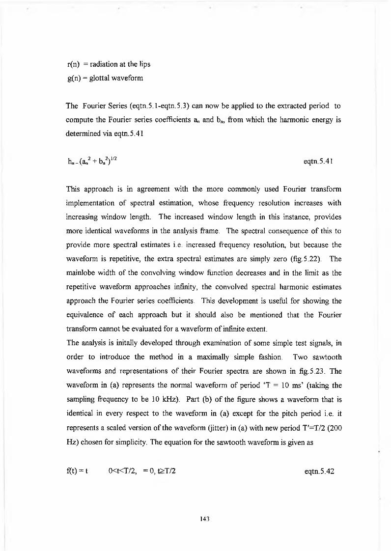
r(n) = radiation at the lips

g(n) = glottal waveform

The Fourier Series (eqtn.5.1-eqtn.5.3) can now be applied to the extracted period to

compute the Fourier series coefficients a„ and bn, from which the harmonic energy is

determined via eqtn.5.41

This approach is in agreement with the more commonly used Fourier transform

implementation o f spectral estimation, whose frequency resolution increases with

increasing window length. The increased window length in this instance, provides

more identical waveforms in the analysis frame. The spectral consequence of this to

provide more spectral estimates i.e. increased frequency resolution, but because the

waveform is repetitive, the extra spectral estimates are simply zero (fig.5.22). The

mainlobe width o f the convolving window function decreases and in the limit as the

repetitive waveform approaches infinity, the convolved spectral harmonic estimates

approach the Fourier series coefficients. This development is useful for showing the

equivalence o f each approach but it should also be mentioned that the Fourier

transform cannot be evaluated for a waveform of infinite extent.

The analysis is initally developed through examination o f some simple test signals, in

order to introduce the method in a maximally simple fashion. Two sawtooth

waveforms and representations o f their Fourier spectra are shown in fig.5.23. The

waveform in (a) represents the normal waveform of period ‘T = 10 ms’ (taking the

sampling frequency to be 10 kHz). Part (b) o f the figure shows a waveform that is

identical in every respect to the waveform in (a) except for the pitch period i.e. it

represents a scaled version o f the waveform (jitter) in (a) with new period T'=T/2 ( 2 0 0

Hz) chosen for simplicity. The equation for the sawtooth waveform is given as

K - i ^ + K 2) 112 eqtn.5.41

f(t) = t 0<t<T/2, = 0, t>T/2 eqtn.5.42

143

win-2561

(a)

freq. (Hz) (b)

4 0 -10

CD -20

o -50 --E03 -80 -

-110--140-L

1000 2000 3000

fireq.(Hz)(c)

— win-8192

4000 5000

fig. 5.22 I n c r e a s i n g w i n d o w l e n g t h f o r F o u r i e r T r a n s f o r m a t i o n o f a p e r f e c t l y p e r i o d i c

w a v e f o r m (A R o s e n b e r g g l o t t a l p u l s e - 1 1 0 H z w a s u s e d ) . B a n d w i d t h s o f h a r m o n i c s

a p p r o a c h i m p u l s e f u n c t i o n s i .e . t h e t r a n s f o r m a p p r o a c h e s t h e s e r i e s c o e f f i c i e n t s .

144

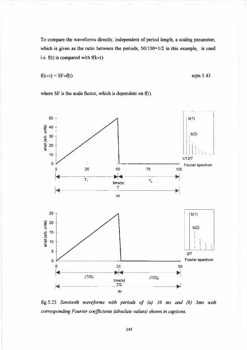
To compare the waveforms directly, independent o f period length, a scaling parameter,

which is given as the ratio between the periods, 50/100=1/2 in this example, is used

i.e. f(t) is compared with f(kxt).

f(kxt) - SFxf(t)

where SF is the scale factor, which is dependent on f(t).

eqtn.5.43

Ti - M -tim e(s)

T

(a)

(T/2),Xtim e(s)

T/2

(b)

(T/2)2

fig.5.23 S a w t o o t h w a v e f o r m s w i t h p e r i o d s o f ( a ) 10 m s a n d (b ) 5 m s w i t h

c o r r e s p o n d i n g F o u r i e r c o e f f i c i e n t s ( a b s o l u t e v a lu e s ) s h o w n i n c a p t i o n s .

145

For the particular case o f the sawtooth waveform, chosen to have a positive slope o f

one, the scale parameter and scale factor are equal and division by the scale factor, ‘k’

according to eqtn.5.44 is required.

f(kxt) = kxf(t)= kx(t) eqtn.5.44

Therefore, if the waveforms are identical in every respect except period length, scaling

the waveforms with respect to each other eliminates the jitter component (eqtn.5.45).

This is easily illustrated with reference to fig.5.23 and eqtn.5.45 and comparing the

waveforms at, for example, point t=50 from (a) (T) which gives fC50)-

(f(l/2x50))/(l/2)=0. For more typical pitch perturbation values we consider a 2% jitter

signal, the perturbed signal having a period of 10.2ms (~98Hz). Subtracting the re­

scaled signal as above gives f(t)-f(1 0 2 / 1 0 0 xt)/(1 0 2 / 1 0 0 ) = 0 , where ‘t ’ is evaluated at

it’s usual discrete sample value points. Therefore, for a direct comparison between

periods, the re-scaled signal must be evaluated at non integer locations and hence an

interpolation algorithm is required.

And substituting into eqtn.5.45 gives f(t)-finter(kxt)/k=f(t)-f(t)=0 as before.

The method as outlined above, in conjunction with the Yumoto et al technique

(eqtn.5.37) forms the basis o f a jitter free harmonic to noise ratio measurement.

However, the need for pitch dependent, pitch synchronous interpolation is avoided by

viewing the signals in the Fourier domain.

In the above development for the sawtooth waveform, a scale factor (SF), which

simply turned out to be the equal to the scale parameter (k), was required in order to

compare two identical waveforms which differed only in period. In general the SF is

dependent on the function being scaled. It is o f interest to consider the scaling o f

f(t)-f(kxt)/k = f(t)-kxf(t)/k= 0 eqtn.5.45

f int e r ( i ) = / ( Z ) + ( / ( * ' + 1 ) - / ( / ' ) ) X k eqtn.5.46

146

cosines, firstly, because the analytical expression for the glottal pulse model consists of

cosine terms and secondly, and more importantly, it provides motivation for an

alternative frequency domain scaling scheme. Re-scaling cosines gives

cos(co'kt) = cos(cot) eqtn.5.47

where © = 211/100 and ©'=211/50, k=50/100

and t is the discrete time unit or sample point

From eqtn.5.47 it is observed that amplitude normalisation is no longer required. This

is similarly true for our glottal pulse model whose analytic expression consists o f two

cosine terms. In applying the Fourier Series, any periodic waveshape can be

represented as the sum o f sine and cosine terms (eqtn.5.1) and utilising eqtn.5.47 to

alter the harmonic frequencies it can be seen that any two waveforms that are identical

in every respect excepting period length will have Fourier coefficients that bear the

same relationship to each other, spaced at an integral number times the inverse o f their

period. The scale factor is simply the period length. Therefore implementing the

scaling in the frequency domain removes the need for a priori knowledge of

complicated scaling factors.

Expansion in the time domain results in frequency domain compression and an increase

in amplitude, due to the length o f the period. This “time compression-frequency

expansion” property (eqtn.5.48) o f the Fourier series is illustrated by the captions

showing Fourier spectra in the top right hand comer o f fig. 5 .23 (a) and (b).

eqtn.5.48

f - frequency, k - scaling parameter

F- Fourier series coefficient, t - discrete time

From eqtn.5.48, if the waveshapes are identical in all aspects except for period, T, then

the Fourier coefficients (i.e. the harmonic amplitudes for each period), are in direct

relation to one another (fig.5.23 (a) and (b) (captions))). For our 100 Hz and 200 Hz

cosine waves eqtn.5.48 has harmonics spaced at 1/T and 1/T' as expected. For more

general functions, if we compare the normalised (i.e. divided by the window length)

harmonics for T with those o f T , they should be identical i.e.

h(nx l/T)-h(nx 1/T') = 0 eqtn.5.49

where h(n) = n“ 1 harmonic

In this manner we are comparing the waveforms based by harmonic number as opposed

to the more usual comparison between ‘same frequency’ location. For the sawtooth

waveform the signal f(t) can be time shifted for ‘oddness’ about x= 0 i.e. f(t) = -f(t) and

the waveform can then be written in terms o f the Fourier series coefficients as

2 1 1/ ( t ) = ——(s in co t - — sin 2 co t + —sin 3 co tJ n 2 3

— sin 4 co t + 4

eqtn.5.50

with cosine terms equal to zero. A scaled version is then simply obtained by

substituting o'= kx© for co. The amplitude coefficients for the sawtooth waveform

have a ‘1/x’ characteristic and the energy (eqtn.5.41) therefore follows a ‘1/x2’ curve

i.e. the spectrum drops off at 6 dB per octave beginning at the fundamental. The

magnitude o f the Fourier coefficients as opposed to the energy is shown in the captions

in fig.5.23 and fig. 5.24 for ease o f illustration. The second advantage o f this approach

is that the need for interpolation has also been removed. Adding the spectra according

to harmonic number is also o f benefit for considering the average glottal flow

characteristics.

Shimmer is also conveniently removed using the pitch synchronous approach. If the

waveform is normalised pitch synchronously (in either domain) then the problem is

immediately removed. Note that here we have considered shimmer to mean that the

waveform is the same in every respect except amplitude at every point in the cycle.

Therefore, this approach enables us to directly compare scaled periods and hence forms

148

the basis o f a measurement technique that can perform an harmonic intensity analysis

which is independent o f jitter and shimmer. In order to obtain the harmonic to noise

ratio, the pitch synchronous harmonics are averaged according to harmonic number

(not frequency location) to form an average harmonic spectrum. The average

harmonic spectrum is then subtracted from the individual pitch synchronous spectra in

order to obtain the spectral noise estimate and hence the H/N ratio

HN

L M

1 j___________L M

X X ( h i ( T j ) - hi(AV) ) 2

eqtn.5.51

hj(Tj) = 1th harmonic of j* spectrum and

hi(AV) = average of i1*1 harmonic

M = total number o f spectra

L = total number o f harmonics

T = time

Based on our development, if hi(Tj)-hi(av) * 0 , then either a wave shape change has

occurred or additive noise is present in the signal i.e. eqtn.5.51 provides jitter and

shimmer free harmonic to noise ratios, where the jitter component has resulted from

waveforms that are identical in every respect except for different periods. We will term

this scaled jitter.

In order to introduce the method in it’s most basic form we have carried out the

analysis on simple waveshapes, including the glottal waveform. Now we consider the

important deviation that is introduced when analysing the output speech waveform.

This occurs as a result of adding by harmonic number as opposed to exact frequency

location. The problem arises as a result o f the harmonic-formant interaction1,29. If we

had developed the technique using the output waveform and considered the waveforms

to be the same in every respect except period we would have been dealing with

waveforms that are impossible to realise in practice. The fundamental frequency,

ft) = 1/T. governs the harmonic source spectrum frequency locations. The amplitudes

149

of these harmonics are modified on passing through the vocal tract filter. For the

output waveform therefore, two cycles cannot be the same in every respect except for

a period difference as they receive different resonant contributions. We are assuming,

of course, that the vocal tract resonance configuration is exactly the same in each case.

In the frequency domain we see that the slight offset in harmonic structure leading to a

slightly different resonance contribution to the harmonic output spectrum. Therefore

the jitter has effectively been turned into harmonic shimmer. It is interesting to note

that jitter cannot exist independently o f shimmer for the output radiated speech

waveform. Through comparison o f typical jitter values for normal (0 -l% ) 3 0 (and

pathological) voices with the resonant bandwidths for the first five formants

(Table.5.3) we can try to estimate the magnitude of the effect. The relationship

between the location o f the fundamental and formant locations must also be taken into

consideration. A correction scheme could then be developed based on a correlation

between jitter, for a given ft) and the resultant ‘harmonic shimmer’.

FORMANT FREQUENCY BANDWIDTH

1 st 650.3 94.1

2 nd 1075.7 91.43 rd 2463.1 107.4

4th 3558.3 198.7

5thl.-.-t-.-r ---------------------------=SS

4631.3 89.8

Table.5.3 Formant data fo r Russian vowel a /from Font16

Another, ultimately more useful, approach is to use pitch synchronous inverse filtering.

Rosenberg3 1 has obtained excellent results for inverse filtering based on pitch

synchronous analysis. The method as introduced by Mathews et al3 2 who state “the

contributions from the vocal tract can be uniquely separated and examined” is to first

estimate the model parameters defined by H(coj) = R(iûJ)V(cOj)G(cOj), where R , V and G

indicate frequency representations of radiation at the lips, the vocal tract and glottal

waveform respectively. Values are computed for H(cc>j) and matched to the spectrum

150

of the waveform under investigation. The parameters are then adjusted so as to

minimise the error. The spectrum of the glottal pulse waveform is then computed

according to

G(k) =

— k

Xn(eJNp )j £ L k

R ( e Np )V (e Np )

,0 < k < N P - 1 eqtn.5.52

where N p is the number o f samples in the p* period.

Therefore the pitch synchronous spectral approach not only allows a convenient means

for eliminating jitter and shimmer artifacts from the signal but can also be used as a

method for inverse filtering. The result is important for our development in that it we

can combine the two, first obtaining the glottal frequency spectra according to

eqtn.5.51 and therefore nullifying the harmonic-formant interaction effects and then

applying the H/N ratio (eqtn.5.50). It is a convenient arrangement in that we are using

the same analysis techniques. Also, o f course, the inverse filtering not only eliminates

the effects o f the formant frequencies on the H/N ratio but also supplies the glottal

spectrum (and pulse, if required).

An objection may be made to calling the approach pitch synchronous in that ( from

eqtn5.50) an average o f several cycles is required in order to obtain our estimate. A

slight modification o f the equation however gives us the harmonic to noise ratio based

on the difference in consecutive spectra. A combination of such approaches may

provide the optimum approach. Obtaining the spectrum pitch synchronously allows us

to take a lot o f measurements on the signal and as stated in section 5.3.5, opens up the

possibility o f making spectral measurements specifically related to vibratory events.

In our development, the jitter artifact was considered to result form a waveform

identical in every respect with it’s neighbouring waveform except for period

differences. We have call this scaled jitter. Several possibilities exist for changing the

pitch period other than simply scaling the periods. Fig.5.24 illustrates some examples.

It can be imagined that the vibratory mechanism is functioning correctly but that due to

some abnormality in tissue properties o f the folds that consecutive closure events occur

151

Q.E<0

Titim e(s)3T/4

(a)

fig. 5.24 (a) P e r i o d c h a n g e d u e t o s h o r t e n i n g o f th e c l o s e d p h a s e . S p e c t r a l e n v e l o p e i s

m a i n t a i n e d a n d f o r t h e s a w t o o t h w a v e f o r m s i n c e t h e F o u r i e r c o e f f i c i e n t s a r e 1 / x th e

r e l a t i v e h e i g h t s o f h a r m o n i c s a r e a l s o m a i n t a i n e d , (b) O t h e r g l o t t a l e v e n t s t h a t m a y

b e th e c a u s e o f p e r i o d c h a n g e s w i t h t h e r i s i n g p a r t o f t h e w a v e f o r m c o r r e s p o n d i n g to

g l o t t a l a b d u c t i o n w h i c h p r i m a r i l y i n f l u e n c e s t h e l o w f r e q u e n c y e n d o f t h e s p e c t r u m .

T h e f a l l i n g e d g e c o r r e s p o n d s t o a d d u c t i o n w h i c h m a i n l y a f f e c t s t h e u p p e r p a r t i a l s .

in quite a random fashion. This case is illustrated in fig.5.24(a) where the open phase

remains exactly the same but the closed phase is either elongated or truncated with

respect to normal. Rothenberg33 has considered a somewhat similar example of

152

aperiodicity where “the vocal fold vibrations are periodic, but an irregular mucous

bridge is making the onset o f the airflow aperiodic”. Ladefoged34, in attempting to

provide a jitter free index representing the random noise components associated with

breathiness proposed using “only part o f a cycle and compare(d) it with the

corresponding part o f the next cycle”. This technique, seems applicable for use on

glottal waveforms with differing closed phases. Although, for use on the output

radiated speech waveform the harmonic-formant interaction will also be present. The

spectral consequence of changing the closed phase is to change the relative height of

the harmonics. However, the spectral envelope remains the same and therefore “zero-

padding” 2 1 the periods until they are o f equal length will regain the relative ‘harmonic’

strengths. Possible mechanisms for the aforementioned scaled jitter might include

differences in tension o f the thyroarythenoid or cricothyroid muscles or differences in

the mass o f the folds taking part in the vibration from cycle to cycle. The period may

also change due to a change in adductory or abductory function (fig.5.24(b)) which

may result from changes in cricoarythenoid activity. Other possible mechanisms are

found in cases involving vocal pathology where the presence o f vocal fold nodules or

mass lesions give rise to aperiodicities and turbulent flow. It is of considerable interest

to spectrally characterise these conditions.

List 1-7 provides the basis for a possible algorithm for investigating glottal

characteristics.

1 . If |hi(T)-hiAv| in eqtn.5.51 gives a value o f zero then there is no additive noise

present in the signal, no change in open quotient (OQ - open time to closed time in one

period o f oscillation) and no change in waveshape.

2. ‘noise’ present indicates either (a) additive noise, (b)OQ has changed or (c)

waveshape change.

3. Check for (b) spectral envelope may be the same, therefore ‘zero pad’ to make

periods equal and calculate |hizc-havzc|, where hiy£ is the i1*1 harmonic for the spectrum

derived form the ‘zero padded’ waveform.

4. If noise ^ 0 then

153

1 . a) or c)

2 . a) |hi-hav| difference is constant for all hi.

3. Check for (c) abduction(look for lower f changes), adduction(tilt - look for higher f

changes)

For more advanced procedures matching the spectral changes with the LF model is the

required approach28. In the actual implementation the pitch period was extracted

according to the method indicated in fig.5.21. The number o f points taken for

calculating the partial sum of the Fourier series is given by

f_cut/fsamx2xmedian(period), where f_cut=3800 Hz (cut off frequency o f low pass

filter) and fsam=10 kHz (sampling frequency).

5 . 4 R e s u l t s :

In this section an examination and interpretation o f the main results obtained from the

present implementations o f the methods detailed in the last section is given and

compared to the results obtained from the original analysis. The order o f presentation

is the same as in the previous section. The analysis programs were run on all synthesis

files and on the patient and normal data. A presentation of all the results is not possible

due to the number o f ratios returned from all programs. In our systematic manner o f

evaluating the H/N ratio techniques we firstly ran the program on the synthesis files

with three levels o f additive noise o f std. dev. 4%, 8 % and 16% for six values of

fundamental frequency (fO) in equal steps from 80 to 350 Hz. If the results from this

analysis were encouraging the response o f the ratio with respect to the jitter and

shimmer files was examined. The potential diagnostic strength o f the ratio was then

evaluated by examining the ratio with respect to the patient/normal data set. In each

section that follows the H/N ratio refers to the H/N ratio calculated by that method e.g.

the harmonic to noise ratio for the Kojima technique is given by eqtn.5.36,

section5.3.6 and the results are given in section 5.4.6.

154

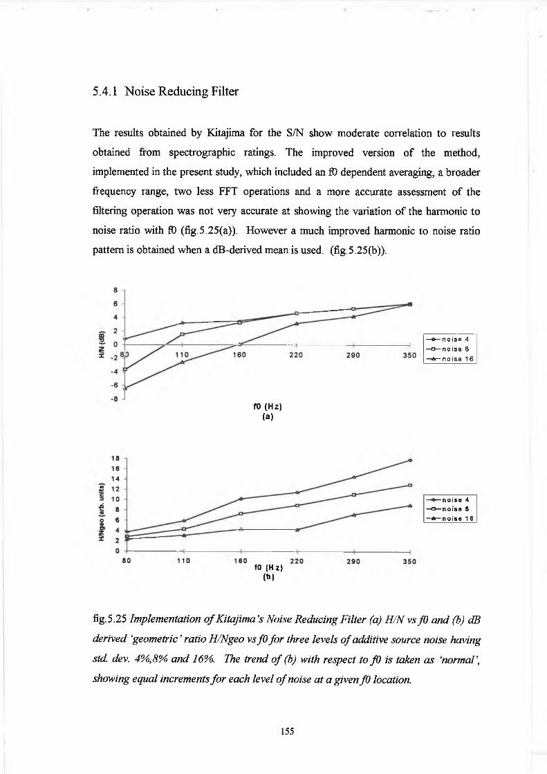
5.4.1 Noise Reducing Filter

The results obtained by Kitajima for the S/N show moderate correlation to results

obtained from spectrographic ratings. The improved version of the method,

implemented in the present study, which included an fO dependent averaging, a broader

frequency range, two less FFT operations and a more accurate assessment of the

filtering operation was not very accurate at showing the variation of the harmonic to

noise ratio with fO (fig.5.25(a)). However a much improved harmonic to noise ratio

pattern is obtained when a dB-derived mean is used, (fig.5.25(b)).

fO (Hz) (a)

—o— n o is e 4

—a — n o is e

CO

- A — n o is e 1 6

fO (Hz) < b)

— n o i s e 4 —a — n o is e 8

■ * n o is e 1 6

fig.5.25 I m p l e m e n t a t i o n o f K i t a j i m a ’s N o i s e R e d u c i n g F i l t e r ( a ) H / N v s f O a n d ( b ) d B

d e r i v e d ‘g e o m e t r i c ’ r a t i o H / N g e o v s f O f o r t h r e e l e v e l s o f a d d i t i v e s o u r c e n o i s e h a v i n g

s td . d e v . 4 % ,8% a n d 1 6 % . T h e t r e n d o f ( b ) w i t h r e s p e c t t o f O i s t a k e n a s ‘n o r m a l ’,

s h o w i n g e q u a l i n c r e m e n t s f o r e a c h l e v e l o f n o i s e a t a g i v e n f O lo c a t io n .

155

The trend in part (b) of fig.5.25 showing H/Ngeo vs fD is explained in the next section

and for now it is simply considered to represent normal. It can be seen that equal

increments in H/Ngeo occur for increases in additive noise levels at a given frequency

location. The improvement in representing the noise increases is similarly shown in

figures 5.26(a) and (b).

(a)

additive noise (std.dev.1%-32%)(b)

fig.5.26 I m p l e m e n t a t i o n o f K i t a j i m a ’s N o i s e R e d u c i n g F i l t e r ( a ) H / N v s a d d i t i v e n o i s e

a n d ( b ) d B d e r i v e d ‘g e o m e t r i c ’ r a t i o H / N g e o v s a d d i t i v e n o i s e . T h e H / N g e o d i s p l a y s

a m o r e r e g u l a r r e s p o n s e w i t h r e s p e c t t o e q u a l i n c r e m e n t s o f a d d i t i v e s o u r c e n o i s e .

In (b), for five doubling in noise levels there is a corresponding decrease of about 2 dB

per doubling. The improvement here is due to the fact that a dB spectrum was used at

the outset before averaging. A similar result would have been obtained if we had left

the original spectrum and summed all values greater than the moving average and then

taken the dB values (not with respect to the noise). It is interesting to note that

156

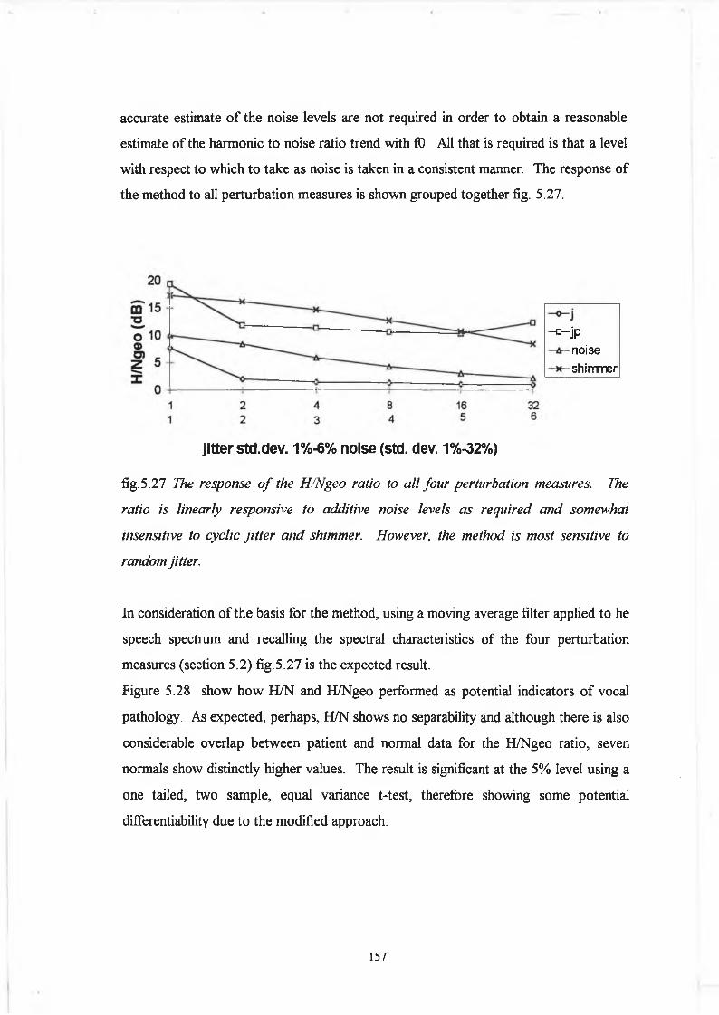
accurate estimate of the noise levels are not required in order to obtain a reasonable

estimate of the harmonic to noise ratio trend with fO. All that is required is that a level

with respect to which to take as noise is taken in a consistent manner. The response of

the method to all perturbation measures is shown grouped together fig. 5.27.

-o -jpnoise

shimmer

jitter std.dev. 1%-6% noise (std. dev. 1%-32%)

fig.5.27 T h e r e s p o n s e o f t h e H / N g e o r a t i o to a l l f o u r p e r t u r b a t i o n m e a s u r e s . T h e

r a t i o i s l i n e a r l y r e s p o n s i v e t o a d d i t i v e n o i s e l e v e l s a s r e q u i r e d a n d s o m e w h a t

i n s e n s i t i v e to c y c l i c j i t t e r a n d s h i m m e r . H o w e v e r , th e m e t h o d i s m o s t s e n s i t i v e t o

r a n d o m j i t t e r .

In consideration of the basis for the method, using a moving average filter applied to he

speech spectrum and recalling the spectral characteristics of the four perturbation

measures (section 5.2) fig.5.27 is the expected result.

Figure 5.28 show how H/N and H/Ngeo performed as potential indicators of vocal

pathology. As expected, perhaps, H/N shows no separability and although there is also

considerable overlap between patient and normal data for the H/Ngeo ratio, seven

normals show distinctly higher values. The result is significant at the 5% level using a

one tailed, two sample, equal variance t-test, therefore showing some potential

differentiability due to the modified approach.

157

0.6 1 1.4 1.8 2.2 2.6 3H/N (dB)

(a)

1.4 1.8 2.2 2.6 3 3.4 3.8 4.2 4.6 5 5.4HNgeo (dB)

(b)

fig. 5.28 P e r f o r m a n c e o f (a) H / N r a t i o a n d (b) H Z N g e o a s p o t e n t i a l i n d i c a t o r s o f v o c a l

p a t h o l o g y f o r t h e d a t a s e t - 1 3 p a t i e n t s ( v a r y i n g p a t h o l o g i e s ) a n d t w e l v e ‘n o r m a l s

5.4.2 Relative Harmonic Intensity (Hr)

Hiraoka’s implementation stresses the fact that a high relative fD amplitude which is

known to be a good indicator of breathiness may be missed by conventional harmonic

to noise ratio estimates. This echos what we have said in section 5.2 regarding the fact

that the waveshape could be the same from period to period and therefore have a high

harmonic to noise ratio and yet could still show considerable pathology due to the

unusual, although consistent waveshape. The Hr ratio as defined in eqtn.5.23 guards

against missing this anomaly. Our implementation sticks closely to the Hiraoka method

although they have failed to state how the harmonic energy estimate was calculated.

Their method was tested on a group of 36 normals and 30 patients. Improved

separability with Hr as opposed to Sr was reported. Figure 5.29 shows the Hr index

158

100

80

g 60X 40

20

080 110 160 220 290

fO (Hz)(a)

fig. 5.29 V a r i a t i o n o f H r ( % ) i n d e x w i t h f O f o r t h r e e l e v e l s o f a d d i t i v e n o i s e

plotted against fO for three levels of additive noise. The trend for the Sr ratio is very

similar (not shown). As stated previously, the trend of increased harmonic to noise

ratio with increasing fO is explained in detail in section 5.5. The Hr ratio for the

patient/normal data are shown in fig. 5.30. The Hr value showed greater separability

than the Sr index (not shown) but considerable overlap still remains with the result not

being significant at the 5% level using the one-tailed, equal variance, two sample,

student’s t-test.

350

0 10 20 30 40 50 60 70 80 90 100

Hr (%)

fig.5.30 D i f f e r e n t i a b i l i t y p e r f o r m a n c e o f H i r a o / c a 's H r i n d e x f o r t h e p a t i e n t ( 1 3 ) /

n o r m a l ( 1 2 ) d a t a s e t . T h e r e s u l t i s n o t s i g n i f i c a n t a t t h e 5 % l e v e l ( o n e - t a i l e d s t u d e n t ’s

t - t e s t )

159

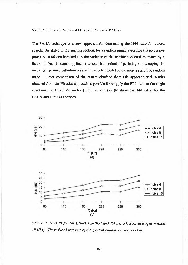
5.4.3 Periodogram Averaged Harmonic Analysis (PAHA)

The PAHA technique is a new approach for determining the H/N ratio for voiced

speech. As stated in the analysis section, for a random signal, averaging (n) successive

power spectral densities reduces the variance of the resultant spectral estimates by a

factor of 1/n. It seems applicable to use this method of periodogram averaging for

investigating voice pathologies as we have often modelled the noise as additive random

noise. Direct comparison of the results obtained from this approach with results

obtained from the Hiraoka approach is possible if we apply the H/N ratio to the single

spectrum (i.e. Hiraoka’s method). Figures 5.31 (a), (b) show the H/N values for the

PAHA and Hiraoka analyses.

fO (Hz)

-o—noise 4 - a - noise 8 - a - noise 16

-noise 4 -noise 8 -noise 16

fO (Hz)(b)

fig.5.31 H / N v s f O f o r ( a ) H i r a o k a m e t h o d a n d (b ) p e r i o d o g r a m a v e r a g e d m e t h o d

( P A H A ) . T h e r e d u c e d v a r i a n c e o f t h e s p e c t r a l e s t i m a t e s i s v e r y e v id e n t .

160

The benefit of overlap and averaging is immediately apparent in the PAHA case. The

results reflect more accurately the noise levels present in the voice signal due to more

consistent spectral estimates. Figure 5.32 shows the H/N ratio plotted with respect to

the perturbation measures.

jitter (1 %-6% std.dev.) shimmer and noise (1%-32% std.dev.)

(a)

30

-sh im m er

-n o ise

-jP-j

jitter std.dev. 1%-6% noise (std. dev. 1%-32%) (b)

fig. 5 .32 (a) P e r i o d o g r a m a v e r a g e d h a r m o n i c a n a l y s i s ( P A H A ) w i t h H / N r a t i o f o r th e

f o u r p e r t u r b a t i o n m e a s u r e s o f a d d i t i v e n o i s e , c y c l i c j i t t e r ( jp ) , r a n d o m j i t t e r ( j ) a n d

s h i m m e r (b) w i t h H / N 1 4 r a t i o - l i m i t i n g th e f r e q u e n c y r a n g e f r o m 1 - 4 k H z

The result (fig.5.32 (a)) is similar to the modified Kitajima approach (fig.5.27). The

method is very sensitive to random jitter variations, even at 1% std. dev. random jitter.

The noise levels are reflected well and the ratio is somewhat insensitive to shimmer.

Again, these results are in agreement with and can be explained by the spectral

characterisation development in section 5.2.

161

In section 5.2 the motivation for different ratios, reflective of perceptual and physical

characteristics was developed. Three new ratio types were introduced with the PAHA

technique, corresponding to limiting the frequency range (H/N 14-harmonic to noise

ratio for frequencies between 1 to 4 kHz - fig.5.32 (b)), perceptually based ratios

(H/Ngeo and H/Ngeo 14-geometric means - fig. 5.3 3) and source correlated ratios (HNs

- fig.5.34).

jitter std.dev. 1%-6% noise (std. dev. 1%-32%)

fig. 5.3 3 G e o m e t r i c d B m e a n r a t i o v s t h e f o u r p e r t u r b a t i o n m e a s u r e s o f j i t t e r ( j) ,

s h i m m e r ( s h m ) , c y c l i c j i t t e r ( j p ) a n d a d d i t i v e n o i s e (n ) .

-noise 4 -noise 8 -noise 16

fO (Hz)

fig.5.34 V a r i a t i o n o f H / N s s o u r c e r a t i o w i t h f O f o r t h r e e l e v e l s o f a d d i t i v e n o i s e .

N o t e t h e v a r i a t i o n w i t h f O i s c o n s i d e r a b l y r e d u c e d .

The ability of all the above mentioned ratios at separating the patient and normal data is

shown in figures 5.35(a),(b) and 5.36 (a), (b) and (c).

162

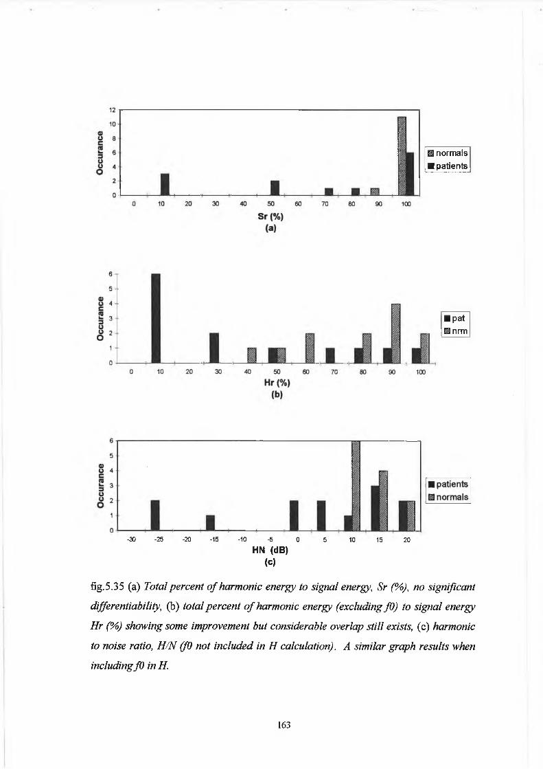
B3 normals ■ patients

■ pat Enrm

-30 -25 -20 -15 -10 -5 0 5 10 15 20

HN (dB)(c)

fig.5.35 (a) T o t a l p e r c e n t o f h a r m o n i c e n e r g y t o s i g n a l e n e r g y , S r (% ) , n o s i g n i f i c a n t

d i f f e r e n t i a b i l i t y , (b) t o t a l p e r c e n t o f h a r m o n i c e n e r g y ( e x c l u d i n g fO ) t o s i g n a l e n e r g y

H r ( % ) s h o w i n g s o m e i m p r o v e m e n t b u t c o n s i d e r a b l e o v e r l a p s t i l l e x i s t s , (c) h a r m o n i c

t o n o i s e r a t io , H / N (fO n o t i n c l u d e d i n H c a l c u l a t i o n ) . A s i m i l a r g r a p h r e s u l t s w h e n

i n c l u d i n g f O i n H .

163

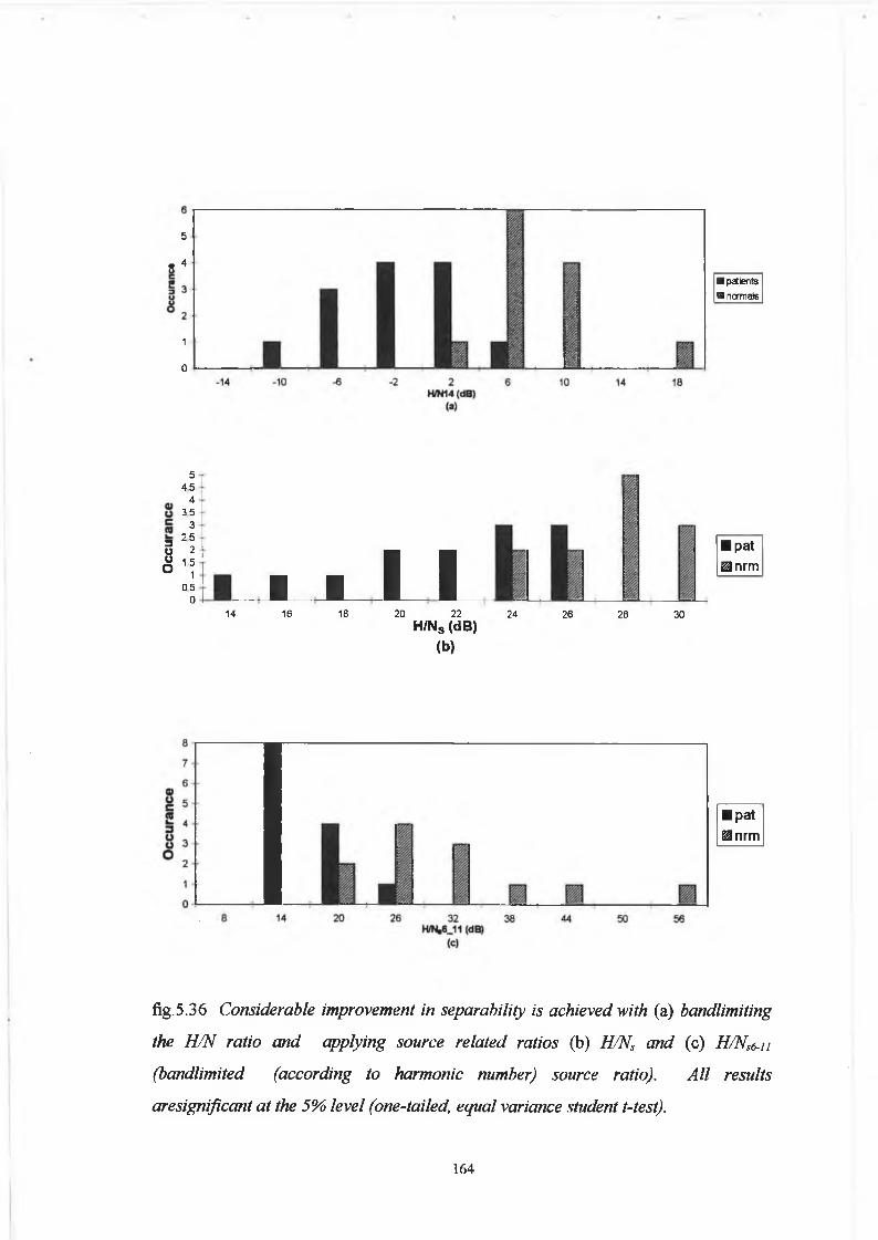
• 4u

5

1

0

Q B 0 i16 18 20 22 24 26 28 30

H/Ns (dB)(b)

3OoO

5 4 5

4 35

3 25

2 1 5

1050

14

■ pSients Bnarrate

■ pat ^nrm

■ pat■ nrm

fig.5.36 C o n s i d e r a b l e i m p r o v e m e n t i n s e p a r a b i l i t y i s a c h i e v e d w i t h (a) b a n d l i m i t i n g

t h e H / N r a t i o a n d a p p l y i n g s o u r c e r e l a t e d r a t i o s (b) H / N , a n d (c) H / N s6- u

( b a n d l i m i t e d ( a c c o r d i n g t o h a r m o n i c n u m b e r ) s o u r c e r a t io ) . A l l r e s u l t s

a r e s i g n i f i c a n t a t t h e 5 % l e v e l ( o n e - t a i l e d , e q u a l v a r i a n c e s t u d e n t t - te s t ) .

164

5.4.4 Normalised Noise Energy (NNE)

In determining the NNE as defined in eqtn.5.31, Kasuya et al examined five frequency

regions for investigating vocal pathology. They found 1-5 kHz to provide the highest

degree o f separability. We have chosen 1-4 kHz (NNEi4) based on this finding as the

cut off frequency o f the low pass filter was 4 kHz. Their ratio was tested on an

extensive set o f pathological voices (186) of varying etiologies and 64 normals. The

error rate reported for normals was 9.4 % and 24.2 % in the case o f pathology.

Nonetheless, they found their method to be superior to Hr (Hiraoka) and H/N

(Yumoto) at separating glottic cancer patients from normals with NNE giving

approximately half the number o f errors as the other two methods. NNE is shown for

the synthesis data with increasing fD in fig.5.37.

-n o is e 4

-n o is e 8

-n o is e 1 6

fig.5.37 NNE vs fO fo r three levels o f additive noise. Approximately equal intervals

fo r each increase in noise level at a given fO location.

The response o f NNE to the four perturbation measures (not shown) is very similar to

the PAHA response, showing a linear response to noise but sensitive to jitter. In it’s

ability to separate our patient/normal set, NNE proved to be a rather poor indicator

whereas NNEi4 showed good separability (fig.5.38).

One possible point to query about this study is that samples were taken at stable pitch

and increased loudness. Samples providing the smallest NNE were taken as

representative for that person. But o f course the increased loudness causes an overall

change in the spectral composition with a decrease in the first formant bandwidth,

165

5

-20 -15 -10 -5 0 5NNE (dB)

(a)

-15 -13 -11 -9 -7 - 5 - 3 - 1 1 3 5

NNE (dB)(b)

fig.5.38 (a) N N E a n d (b) N N E 14 ( b a n d l i m i t e d f r o m b e t w e e n 1 a n 4 k H z ) . O n l y th e

l a t t e r i s s i g n i f i c a n t a t t h e 5 % l e v e l ( s t u d e n t ’s t - t e s t ) .

evidenced in the time domain pulse by a less rapid decay of the frequency of the first

formant. However, it does raise the question of what the best criterion should be for

obtaining samples. Whatever is chosen, the format must necessarily be of a simple

nature, be accurately rated perceptually and cause minimum discomfort to the patient.

5.4.5 Pitch Synchronous (Four Period) Analysis

The Muta et al technique differs from all others in that only the first 16 harmonics are

taken to represent the speech waveform. The justification for this was explained in

section 5.40. As a result of this approach, 1600 Hz is covered for a 100 Hz signal and

3200 Hz is covered for a 200 Hz signal. It is interesting to note that this study uses the

166

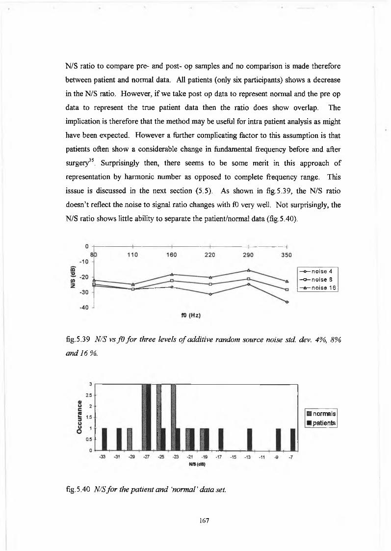
N/S ratio to compare pre- and post- op samples and no comparison is made therefore

between patient and normal data. All patients (only six participants) shows a decrease

in the N/S ratio. However, if we take post op data to represent normal and the pre op

data to represent the true patient data then the ratio does show overlap. The

implication is therefore that the method may be useful for intra patient analysis as might

have been expected. However a further complicating factor to this assumption is that

patients often show a considerable change in fundamental frequency before and after

surgery35. Surprisingly then, there seems to be some merit in this approach of

representation by harmonic number as opposed to complete frequency range. This

isssue is discussed in the next section (5.5). As shown in fig.5.39, the N/S ratio

doesn’t reflect the noise to signal ratio changes with fO very well. Not surprisingly, the

N/S ratio shows little ability to separate the patient/normal data (fig.5.40).

—o— n o ise 4

- o - n o i s e

CO

—a— n o ise 16

fig.5.39 N / S v s f O f o r t h r e e l e v e l s o f a d d i t i v e r a n d o m s o u r c e n o i s e s t d d e v . 4 % , 8%

a n d 1 6 % .

I normals I patients

fig.5.40 N/S for the patient and ‘normal’ data set.

167

5.4.6 Partial Sum of the Fourier Series - Kojima et al

In Kojima’s study, a set of fourteen males and fourteen females were used as normals

and a set of twenty males and ten females comprised the patient data. The results were

compared with spectrographic and auditory impressions. Some overlap was evident

for the data set with normals ranging from 15 to 23 dB and patients ranging from -1.5

to 20.3 dB. The method is attractive due to it’s simplicity in coding, with two points

noise, one point harmonic etc. . However, the method is easily offset due to jitter.

Figures 5.41 (a) and (b) show the measure with respect to fO (for three levels of

additive noise) and the four perturbation measures. The ability of the index at

differentiating between the patient/normal data set is shown in fig.5.43.

fO (Hz)(a)

- o - noise 4

—o— noise 8

—a— noise 16

50

40

5 , 20 z 10

-10

jitter std.dev. 1%-6% noise (std. dev. 1%-32%) (b)

fig. 5.41 R e s p o n s e o f th e K o j i m a H / N r a t i o t o ( a ) f O f o r th r e e l e v e l s o f a d d i t i v e n o i s e

a n d ( b ) t h e f o u r p e r t u r b a t i o n p a r a m e t e r s w h e r e j ’ i n d i c a t e s r a n d o n j i t t e r a n d j p ’

c y c l i c j i t t e r .

- o - noise

- o - shimmer

-»«-jp

168

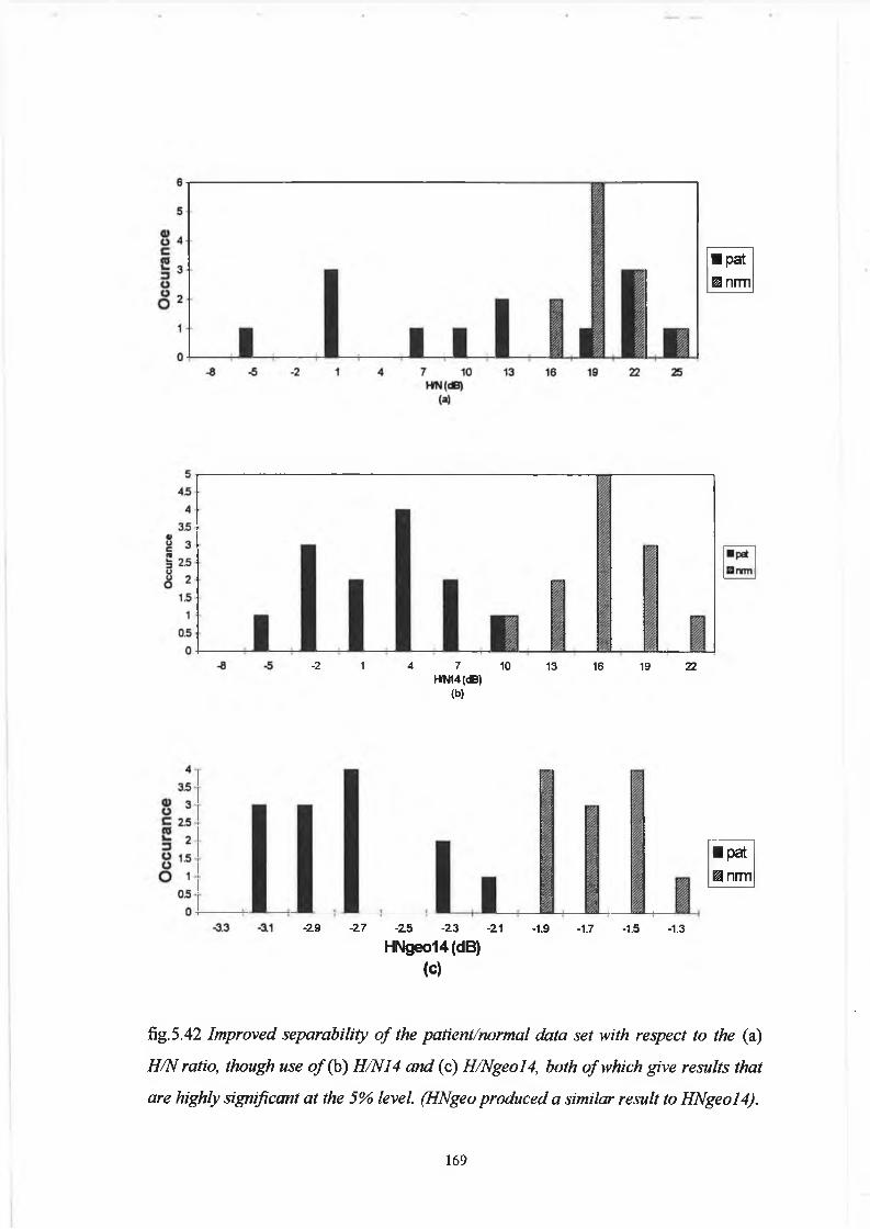
■ pat 0nrm

-2 1 4 7 10HfN14(<B)

(b)

13 16 19 22

-29 -27 -25 -23 -21 -1.9

HNgeo14(dB)(c)

-1.7 -1.5

■ pat & n r m

-1.3

fig. 5.42 I m p r o v e d s e p a r a b i l i t y o f t h e p a t i e n t / n o r m a l d a t a s e t w i t h r e s p e c t t o t h e (a)

H / N r a t io , t h o u g h u s e o f (b) H / N 1 4 a n d (c) H / N g e o l 4 , b o t h o f w h i c h g i v e r e s u l t s t h a t

a r e h i g h l y s i g n i f i c a n t a t t h e 5 % le v e l . ( H N g e o p r o d u c e d a s i m i l a r r e s u l t t o H N g e o l 4 ) .

169

5.4.7 Partial Sum o f the Fourier Series - Two Cycle Analysis

Two cycles of the waveform were taken and moved on one cycle at a time therefore

providing an H/N ratio pitch synchronously. In this manner jitter and shimmer still

contribute to the noise estimates. Again, the method is very appealing by nature of it’s

simplicity. A further advantage is that we can simply go back to the time domain with

either the noise or noiseless signals, simply by disregarding every second Fourier

coefficient in taking the inverse. The response of the H/N ratio with respect to fO and

for additive noise and perturbation measures was essentially the same as for the Kojima

method (fig.5.41). Many new ratios were also investigated, including two dB derived

measures and six source or H/Ns based measures including bandlimited versions. The

performance of a selection of these measures with respect to the patient/normal data

set are shown in fig.5.43 to 5.44. Improved separability is obtained through use of the

source based, perceptually based and bandlimited approaches (H/N not shown-poor

separability).

01ë 5 (05 48 3

I I ■

I p a t

H / N 14 ( d B )(a)

«oc23aë

0 .9 0 .9 1 1.2

H/ N g e o l 4 ( d B )<b)

I p a t

fig.5.43 (a) H / N 1 4 - b a n d l i m i t e d r a t i o a n d (b) H n g e o l 4 - b a n d l i m i t e d p e r c e p t u a l l y b a s e d

r a t i o f o r t h e p a t i e n t / n o r m a l d a t a s e t s . B o t h a r e h i g h l y s i g n i f i c a n t a t t h e 5 % le v e l .

170

22HNs(dBf(a)

34 36

fl> 4

O 2

20 24H/N,6J1 (dB)

(b)

I pat Inrm

28 32

20 24H/Ns14 (dB)

(c)

■ pat E3nrm

fig.5.44 S o u r c e r e l a t e d H / N r a t i o s (a) H /N s , (b) H / N s 6- iu b a n d l i m i t e d a c c o r d i n g to

h a r m o n i c n u m b e r a n d (c) H / N s h , 1 - 4 k H z b a n d l i m i t . A l l m e a s u r e s a r e s i g n i f i c a n t a t

t h e 5 % l e v e l ( s t u d e n t ' s t - t e s t ) .

171

5.4.8 Time Domain Averaging - Yumoto et al

The Yumoto paper reported good separability of their patient (12 males/eight

females)/normal (22 males/20 females) data and the post surgery improvements also

shows good agreement. The H/N ratio for males (average 12.2 dB) did not vary

significantly from the H/N ratio for females (average 11.5 dB) and therefore the sets

were combined and compared with the patient data. Their values for normals ranged

from 7 to 17 dB and pre-op patient data from -15,2 to 9.6 dB, with post-op patient

data ranging from 5.9 to 17.6 dB. It is interesting to note that their patient pre-op

values went as low as -15.2 dB (~30 times more noise than signal) despite the fact that

they could “demarcate pitch periods even in the hoarse voices”. This therefore

suggests that despite having clearly defined pitch markers, the signal behaved very

erratically between these markers i.e. had a very different waveshape from period to

period. Although this type of behaviour may occur in some conditions such as spastic

dysphonia, the more likely explanation is that tracking errors did in fact occur given the

magnitude of the ratio. The response of the H/N index to increases in fD and the

perturbation measures is shown in fig.5.45. Our approach also included a frequency

domain analysis from which the geometric dB mean (H/Ngeo) once again proved to be

superior to the H/N ratio at separating the patient/normal data. In fact the

patient/normal data was completely separated using this method (fig.5.46).

25

0 4-

80 110 160 fO (Hz) 220(a)

290 3S0

Fig. 5.45 (a) R e s p o n s e o f H / N t i m e d o m a i n r a t i o t o c h a n g e s i n f O w i t h t h r e e l e v e l s o f

a d d i t i v e r a n d o m n o i s e w i t h s td . d e v . 4 % , 8 % a n d 1 6 % .

50 T

8 16 32

jitter std.dev. 1%-6% noise (std. dev. 1%-32%)(b)

fig. 5 .45 (b) R e s p o n s e o f th e H / N i n d e x t o t h e f o u r p e r t u r b a t i o n m e a s u r e s o f r a n d o m

j i t t e r - j c y c l i c j i t t e r - j p a d d i t i v e n o i s e a n d s h i m m e r . N o t e t h e r e d u c e d s e n s i t i v i t y o f

t h e m e a s u r e w i t h r e s p e c t t o j i t t e r a c o m p a r e d to a l l p r e v i o u s a n a ly s e s .

In part (b) of fig.5.45, the reduced sensitivity of the H/N index is a result of the fact

that the method is pitch synchronous and also because the median period was used in

estimating the average period (see eqtn.5.37 and eqt.5.38).

<DOc23ÜÜO

I pat.I nrm.

4

3 5

3

2 .5 - ■

2 - ■

1 .5

1

0 .5 4 *

I

H /lrg e o ( d B ) c ( b )

Inrm ■ pat

fig. 5.46 I m p r o v e d s e p a r a b i l i t y o f p a t i e n t / n o r m a l d a t a s e t s u s i n g (b) H / N g e o

( s i g n i f i c a n t a t t h e 5 % l e v e l ) a s o p p o s e d t o (a) t h e t r a d i t i o n a l H / N r a t i o .

173

5.4.9 Pitch Synchronous Harmonic Analysis (PSHA)

This novel procedure was designed to provide a measure that is indicative of noise

levels in pathological vocal qualities, independent of jitter and shimmer perturbations.

Obtaining a spectrum pitch synchronously provides us with several measures including

various shimmer measures and distortion factors as well as the usual spectral measures.

In addition to this it allows comparison with the frequency domain implementation of

the four parameter glottal flow model. Figure 5.47(a) shows the harmonic to noise

ratio plotted with respect to fO for the three levels of additive noise.

m■o

fO (Hz) (a)

16

jitter std.dev. 1%-6% noise (std. dev. 1%-32%)(b)

■noise-4 • noise-8 •noise-16

32

fig. 5.47 (a) T h e u s u a l f O t r e n d w i t h a p p r o x i m a t e l y e q u a l d e c r e m e n t s i n t h e H / N r a t i o

( a t a g i v e n fO ) f o r i n c r e a s e s i n n o i s e le v e l , (b) T h e r e s p o n s e t o t h e p e r t u r b a t i o n

m e a s u r e s s h o w s a m a r k e d i m p r o v e m e n t o n o t h e r m e th o d s .

174

Part (b) of fig.5.47 shows the variation with respect to the perturbation measures. For

the worst cases of jitter and shimmer the H/N ratio is still above 10 dB whereas the

ratio has reaches this index at ~2% std. dev. random additive noise. The effects of

jitter and shimmer on the index has been totally eliminated due to the harmonic formant

interaction process as mentioned in section 5.3.9. The index was also tested on the

glottal source data in order to examine if the index was truly jitter and shimmer free as

hypothesised.

aEra

-jitter-random

- noise

random jitter (std.dev.%)

additive noise (std.dev.%)4 8 16 32

fig.5.48 T h e p e r f o r m a n c e o f t h e p i t c h s y n c h r o n o u s h a r m o n i c t o n o i s e r a t i o

( e q t n .5 .5 1 ) w i t h r e s p e c t t o r a n d o m j i t t e r a n d r a n d o m a d d i t i v e n o i s e o f t h e g l o t t a l

s o u r c e .

The ratio shows a good linear response with respect to the additive noise levels and the

harmonic to noise ratio maintains a level of about 40 dB (with slight variation) up to 6

% std. dev. random jitter. Interpolation of the time domain data, in order to locate the

positive zero crossing before the major peak would reduce the slight variability of the

index. Shimmer was completely eliminated by normalising the waveform prior to

obtaining the spectral estimates and hence gave an infinite harmonic to noise ratio.

For the patient/normal data, the H/N ratio gave poor separability (not shown). The

HZNu ratio gave values ranging from 10 to 20 dB for the normal data and from 0 to

175

7.5 dB for the patient data, therefore completely separating the two data sets (fig.5.49

(a)). The geometric dB mean is shown in part (b) of the figure.

O 3 oO 2

1

0 ■ i l l

I

6 0 10 12 14

H/N14 (dB)(a)

16 18 20

■ pat. ^nrm.

3 5 4 4 5 5 5 5 6 6.5 7 7 5 8

H/Ngeo (dB)(b)

fig.5.49 (a) B c m d l i m i t e d a n d (ty g e o m e t r i c d B m e a n , p i t c h s y n c h r o n o u s h a r m o n i c to

n o i s e r a t io s . B o t h r e s u l t s b e i n g h i g h l y s i g n i f i c a n t a t t h e 5 % l e v e l ( t w o s a m p le , e q u a l

v a r i a n c e , s t u d e n t t - t e s t ) .

The total harmonic, average percentage amplitude perturbation, THAPAP, defined as

THAPAP =

L M-l

i jHav

eqtn.5.53

where hAvis the mean harmonic value taken over all spectra.

176

I

THAPAP is shown for the patient and normal data in fig.5.47(a). Substituting dB

values for hi in the numerator of equation 5.53 and removing the demoninator gives the

total harmonic shimmer index (fig. 5.47(b)). Other indices such as APAP (average

percentage amplitude perturbation-eqtn.5.53 for Is1 harmonic) and distortion factor

(amplitude of fO divided by total signal amplitude) were also examined. However, they

did not perform well at separating the patient/normal data set.

0.3 0.4 0.5 0.6 0.7 0.8

Average percentage harmonic amplitudeperturbation (linear ratio)

(a)

3 4 5 6 7 8

Harmonic Shimmer (dB)(b)

fig.5.50 (a) ( T H A P A P ) T o t a l h a r m o n i c , a v e r a g e p e r c e n t a g e a m p l i t u d e p e r t u r b a t i o n

a n d (b) ( T S H M ) h a r m o n i c s h i m m e r s h o w i n g g o o d s e p a r a b i l i t y o f t h e p a t i e n t / n o r m a l

d a t a s e t , b o t h o f w h i c h w e r e s i g n i f i c a n t a t t h e 5 % l e v e l o f t h e o n e ta i l e d , e q u a l

v a r i a n c e , tw o s a m p l e m e a n , s t u d e n t s t - te s t .

i l l

5.5 Discussion

5.5.1 Variation of Harmonic to Noise Ratio with Fundamental Frequency

for the Synthesis Data : Analysis Considerations

One of the most striking features o f the graphs in the results section is the variation o f

the harmonic to noise ratio with fundamental frequency (fO). All methods except one -

the four period, ‘pitch synchronous’ approach by Muta et al, show this trend o f

increased H/N ratio with fO (see fig.5.31 for example). In fact, with the synthesis files

used by Muta et al, which came from Titze’s SPEAK program36, an fO trend was also

noticed, although it had a different characteristic to the variation shown here. This

variation was simply attributed to the type o f synthesis used. In a report which

determined the harmonic to noise ratio using the cepstrum technique, de Krom37

noticed a similar variation o f H/N ratio as that encountered here i.e. H/N ratio

increased as ft) increased.

In order to investigate possible causes o f the ft) trend, the periodogram averaged

harmonic analysis program (PAHA-section 5.3.3) was used. Of basic concern in

spectral analysis is the resolution required for a certain measurement. Depending on

resolution, different characteristics o f a signal are revealed. Obvious examples o f this

in speech analysis are the narrowband and broadband spectrograms, the former

resolving the harmonic frequencies and the latter showing more gross characteristics

i.e. the formant tract. Due to the coherent addition o f the discrete Fourier transform, it

is the 6 dB bandwidths that determine spectral resolution, as opposed to the 3 dB

criterion o f classical signal analysis12. Two factors determine whether two signals

spaced at given frequency locations will be resolved : (1) the difference in frequency

between the signals and (2) the bandwidth o f the Fourier estimates. Increased

fundamental frequency therefore produces greater separation between the harmonic

locations. The window length (and type) determines the bandwidth o f the Fourier

estimates. Therefore, for a given window length, we might expect different harmonic

resolution with fO variation for the synthesis files and consequently a different H/N

178

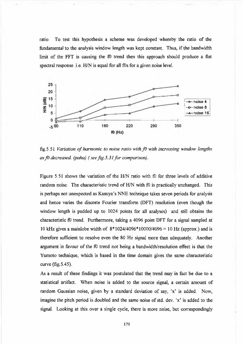
ratio. To test this hypothesis a scheme was developed whereby the ratio o f the

fundamental to the analysis window length was kept constant. Thus, if the bandwidth

limit o f the FFT is causing the ft) trend then this approach should produce a flat

spectral response .i.e. H/N is equal for all fDs for a given noise level.

—©— noise 4 -a -n o is e 8 - a - noise 16

fig.5.51 Variation o f harmonic to noise ratio with fO with increasing window lengths

as fO decreased, (paha) ( see fig. 5.31 fo r comparison).

Figure 5.51 shows the variation o f the H/N ratio with ft) for three levels o f additive

random noise. The characteristic trend o f H/N with fO is practically unchanged. This

is perhaps not unexpected as Kasuya’s NNE technique takes seven periods for analysis

and hence varies the discrete Fourier transform (DFT) resolution (even though the

window length is padded up to 1024 points for all analyses) and still obtains the

characteristic fO trend. Furthermore, taking a 4096 point DFT for a signal sampled at

10 kHz gives a mainlobe width o f 8*1024/4096*10000/4096 = 10 Hz (approx.) and is

therefore sufficient to resolve even the 80 Hz signal more than adequately. Another

argument in favour o f the fO trend not being a bandwidth/resolution effect is that the

Yumoto technique, which is based in the time domain gives the same characteristic

curve (fig.5.45).

As a result o f these findings it was postulated that the trend may in fact be due to a

statistical artifact. When noise is added to the source signal, a certain amount of

random Gaussian noise, given by a standard deviation of say, ‘x ’ is added. Now,

imagine the pitch period is doubled and the same noise o f std. dev. ‘x’ is added to the

signal. Looking at this over a single cycle, there is more noise, but correspondingly

179

more signal, and therefore the signal to noise ratio remains the same. To see why this

may not be the case, a single point in a given cycle is considered (fig.5.52). We are

considering a random, mean zero signal, therefore the mean o f the additive noise

component added to this part of the signal is also zero21.

tim e (s*10e-4)

fig. 5.52 Illustration o f statistical variation o f a single point in the glottal waveform.

The variance o f a single point is equal to the variance o f the signal.

For a given window length, the average we obtain for the point shown in the figure is

better for the higher frequency signals simply because more of them occur in the

analysis frame. Two compensatory factors are required. Firstly, the window length is

(imagine period length 2:1) doubled to compensate for the two to one ratio o f number

of periods per window and secondly the number o f points per period must be

compensated (double again). Therefore, in order to obtain equally accurate estimates

o f the mean for a signal whose periods differ by a 2:1 ratio we must use a four times

longer analysis length for the longer period signal. Neither of these compensations are

necessary, o f course in the perfectly averaged signal. The hypothesis was checked

using the Yumoto technique i.e. the analysis length was determined by the above

mentioned statistical and fO relationship e.g. 160 Hz with 1024 points gives 80 Hz

with 4096 points. However, the characteristic fO trend still remained (fig.5.53) and it

was therefore concluded that the data did not in fact require any special statistical

considerations i.e. the statistical variability is removed using standard analysis lengths

with no special compensatory factors required.

180

-o — noise 4 - a —noise 8 - a - noise 16

fig.5.53 Variation o f harmonic to noise ratio with fO with increasing window lengths

as fO decreases in order to compensate fo r statistical artifacts, (see fig. 5.31 fo r

comparison). (Yumoto Technique).

Further investigations, involving observation o f the source spectra (fig.5.54), revealed

the true nature o f the fO trend. The H/N ratio is plotted for the three levels of noise

versus fO in fig.5.55 for the glottal source files. It can be seen that the signal to noise

ratio o f the source data is in fact equal for all frequencies. It is interesting to note that

fig.5.3.4, the source derived H/N ratio recaptures this linear characteristic. In one

sense therefore it is seen that the H/N variation is due to the synthesis. However, it is

simply due to the greater weight given to the higher frequencies as explained in section

5.2.3 as opposed to any peculiarities due to vocal tract filtering.

30 25

20

I «Z 10 -

80 110—)----------------1—160 220

fO (Hz)290 350

noise 4 -a — noise 8 - a - noise 1 6

fig. 5.54 Periodogram harmonic to noise ratio vs JO for the glottal source data. H/N

reflects the amount o f noise added to the signal at all fundamental frequencies

accurately (i.e. ~<5 dB reduction fo r each doubling o f noise level).

181

ampi

. (d

B)

ampi

. (d

B)

ampi

. (d

B)

0 1000 2000 3000 4000 5000

freq. (Hz)(a)

20

10

0

-10

-40

-500 1000 2000 3000 4000 5000

freq. (Hz)(b)

20 x 10

-10

-20-30

-40

-50

rflW

1000 2000 3000 4000 5000

fireq. (Hz)(c)

fig.5.55 Periodogram analysis o f glottal source data for (a) 80 Hz, (b) 160 Hz and (c)

350 Hz signal with 4% std. dev. additive noise.

182

—o— noise 4 -o-noise 8 - a - noise 16

fO (Hz)(b)

fig. 5.56 Periodogram H/Nu ratio fo r the glottal source data.

This is clearly illustrated if the H/Nu ratio is taken for the glottal source data (fig. 5.55).

The characteristic fO trend is regained. Examination of the source spectra for std. dev.

4 % additive noise for the 80 Hz, 160 Hz and 350 Hz source signals helps provide the

answer for the observed fO trend. For the 80 Hz file the lower partials dominate in the

calculation of the H/N ratio. However, when the signal is bandlimited from between 1

and 4 kHz the resulting H/N ratio is greatly reduced. Considering the 350 Hz file, the

harmonic frequencies are still very prominent in the 1-4 kHz range, only giving a slight

reduction in the H/N ratio.

The basis behind this occurrence was examined in section 5.3.9 when ‘scaled jitter’ was

investigated. The different source signals with different fundamental frequencies can

be viewed as scaled versions o f each other and therefore their relative harmonic

strengths are equal. The first fourteen harmonics for the 80 Hz file have occurred by

1120 Hz whereas the first fourteen harmonics for the 350 Hz file span the complete

frequency range up to 5000 Hz. The harmonic to noise ratio is compared according to

harmonic number in fig.5.56 using pitch synchronous harmonic analysis (psha). The

response with ft) is almost flat. Therefore, as was stated when discussing the Muta et

al technique, there is considerable benefit in considering the signals according to

harmonic number as opposed to frequency range. An obvious objection to this is that

the formant frequency locations differ only by 25 % for male and female speakers

whereas their pitches have an octave difference. Therefore for the output radiated

speech waveform a set frequency range is probably more appropriate. However, for

183

fO (Hz)

—o - noise 4 -a -n o is e 8 —a— noise 16

fig.5.57 Periodogram H/N ratio taking the first 14 harmonics fo r the glottal source

data. Approximately linear but the lower frequencies have slightly higher H/N due to

higher sampling.

inverse filtered or other source related data, analysis by harmonic number is the

preferred approach. Note that in fig.5.55 a spectrum equivalent to the 80 Hz file could

have been obtained for the 350 Hz file if it had been sampled at a frequency that

maintained the same ratio between sampling rate and pitch period (as for the 80 Hz

file). An appropriate sampling frequency is therefore another issue for consideration.

Interpolation could also be used. Kasuya38 has shown that a high sampling frequency

(40 kHz) is required in order to capture the high frequency noise components

accurately. Twenty kHz seems a reasonable compromise between excessive data and

reasonably accurate determination o f the signal. The benefit (H/N ratio unchanged) o f

analysing by harmonic number echos what was stated in section 5.3.9 regarding scaled

signals. It can be seen therefore that the present consideration regarding H/N variation

with fD, the problem o f jitter and shimmer and the question o f inverse filtering, all have

a common solution in the form o f pitch synchronous harmonic analysis.

184

5.5.2 Comparison of Analysis Techniques Based on Spectral

Characterisation of Perturbation with Inferences for Future Development of

Quantitative Analysis

All o f the Fourier techniques (series and transform), except the pitch synchronous

harmonic analysis approach (paha), show considerable overlap for the H/N ratio values

reported for jitter and additive noise. In general the methods are somewhat less

sensitive to shimmer i.e. they reflect shimmer levels accurately. The harmonic to noise

ratios for seven o f the techniques (Kitajima method not shown because scale is

different and two cycle analysis omitted because of it’s similarity to the Kojima

technique) are shown plotted with respect to the four perturbation measures in figures

5.58 to 5 .61. The trend o f the harmonic to noise ratio with respect to the perturbation

measures is readily explained by referring to the spectral characterisation development

in section 5.2.2.

- ”hp— ■—-"hs

“ "ko- - * - ■"psha— * —-"hy

- ”h4—-1—-"n

fig.5.58 Response o f seven o f the analysis techniques to random jitter. The pitch

synchronous harmonic analysis (psha) technique and modified Yumoto (hy) technique

show least sensitivity to jitter, hp-periodogram, hs-Hiraoka, ko-Kojima, h4-Muta, n-

K asuya’s NNE (inverted).

185

The harmonic structure for the random jitter signal is completely missing even for 2 %

standard deviation jitter. Therefore, in estimating the harmonic levels the programs

acquire reduced energy values at nxfD locations and because the ‘noise’ energy in

jittered signals follow the signal properties the energy at between harmonics is o f a

comparable level to the energy at harmonic locations. Both of these effects contribute

to reduced harmonic to noise ratio estimates. Close examination o f the spectra for the

random jitter signals reveals that small amounts o f periodicity reappears in the signal at

locations determined by the standard deviation o f the jitter and the actual fundamental

frequency present. Therefore, some measurement reflecting the reappearance o f

periodicity would reveal whether the reduced harmonic to noise ratio was actually due

to increased levels o f noise or increased levels of jitter.

30

cyclic jitter (%)

fig.5.59 Response o f seven o f the analysis techniques to cyclic jitter. The pitch

synchronous harmonic analysis (psha) technique, modified Yumoto (hy) technique and

Muta method show least sensitivity to cyclic jitter, hp-periodogram, hs-Hiraoka, ko-

Kojima, h4-Muta, n-Kasuya's NNE (inverted).

For cyclic jitter, which is a cardinal symptom o f ‘creaky’ vocal quality, subharmonics

appear in the spectrum. As stated by Fujimura39 if there is a discontinuous shift in

fundamental frequency as sometimes evidenced in creaky voice production, traditional

pitch trackers will try to fit a smoothed curve between fO estimates. This therefore

186

does not reflect the source o f the perturbation very accurately. An alternative

approach is to base the pitch extraction on the spectral properties o f the perturbation as

suggested by Fujimura. Equations 5.10 and 5.11 provide the basis for quantifying the

characteristics o f the subharmonic regimes. Further developments, involving the

application of these equations to successive spectra could provide an indication o f the

onset and offset o f subharmonic production. Note amplitude modulation or cyclic

shimmer would similarly produce subharmonic regimes.

40

35

30

25

I 20I 15

10

5

0

fO (Hz)

fig. 5.60 Response o f seven o f the analysis techniques to additive noise. All methods

reflect the noise levels accurately except fo r the Muta technique, hp-periodogram, hs-

Hiraoka, ko-Kojima, h4-Muta, n-Kasuya 's NNE (inverted).

All analysis programs reflect the level o f additive noise accurately, but as we have seen

in section 5.2.2, the noise levels introduced using random Gaussian noise are

independent o f the signal properties and also have a flat frequency characteristic which

moves upwards (with respect to amplitude). Therefore all methods give false estimates

of harmonic energy at nxfO locations due to noise contributions at these locations.

Observation o f the noise spectra motivates other possible strategies for differentiating

between additive noise and jitter e.g. a calculation o f noise i.e. spectral estimates at

(n+l/2)xf0, in the upper frequency region would reveal the source of the perturbation.

187

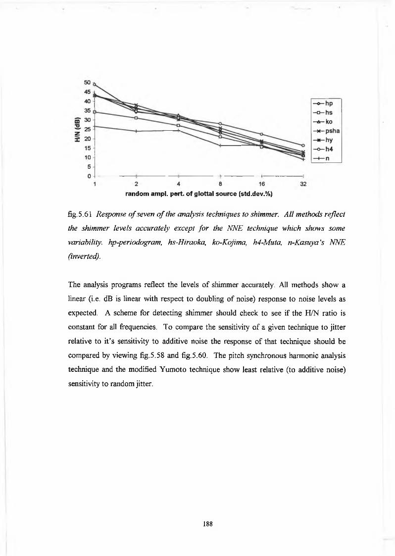
random ampi. pert, of glottal source (std.dev.%)

fig.5.61 Response o f seven o f the analysis techniques to shimmer. All methods reflect

the shimmer levels accurately except fo r the NNE technique which shows some

variability, hp-periodogram, hs-Hiraoka, ko-Kojima, h4-Muta, n-Kasuya’s NNE

(inverted).

The analysis programs reflect the levels o f shimmer accurately. All methods show a

linear (i.e. dB is linear with respect to doubling of noise) response to noise levels as

expected. A scheme for detecting shimmer should check to see if the H/N ratio is

constant for all frequencies. To compare the sensitivity of a given technique to jitter

relative to it’s sensitivity to additive noise the response of that technique should be

compared by viewing fig.5.58 and fig.5.60. The pitch synchronous harmonic analysis

technique and the modified Yumoto technique show least relative (to additive noise)

sensitivity to random jitter.

188

5.6 Conclusion:

If the ultimate goal is to detect or specify the vibratory pattern of the vocal folds from

spectral measures then the contaminating effects of jitter, shimmer and additive noise

must be removed. Presently used harmonic to noise ratio methods provide a ‘catch all’

criterion in evaluating vocal pathologies i.e. the presence o f jitter and shimmer

contribute to the reduced harmonic to noise ratios. An advantage o f this fact is that it

might be useful for characterising the overall state of the voice. However, it reduces

the specificity o f the measure in terms o f describing laryngeal activity.

This problem was addressed using a pitch synchronous harmonic analysis (psha)

technique. The sensitivity o f the resulting H/N ratio to jitter was much less than for

other non-pitch synchronous methods. Similar reductions in jitter sensitivity were

obtained using an adaptation o f the Yumoto technique which employed a median

period for the signal averaging scheme (eqtn.5 .38). Jitter was not completely removed

due to harmonic-formant interactions. However, when ‘psha’ was applied to the

glottal waveform the effects o f jitter were almost completely removed. Shimmer

contributions to the H/N ratio were entirely eliminated in this manner. The advantage

of frequency domain scaling was introduced and it was suggested that more

complicated variations in pitch period could similarly be accounted for by pertinent

frequency domain adjustments.

Basic research is required in order to characterise the nature o f pitch perturbation and

resultant glottal flow characteristics. Examination of pitch synchronous inverse filtered

glottal spectra and waveforms for patients with high jitter scores would lead to better

classification o f the anomaly. Gobi40, Karlsson41 and others have matched inverse

filtered glottal flow waveforms with the flow parameters of LF model in order to

characterise the flow. Recent research has attempted to develop a frequency domain

parameter set o f glottal flow which accepts tape recorded speech data and therefore

avoids the need for phase sensitive recording which can be quite laborious and give

discomfort to the patient. The development o f the ‘psha’ technique, therefore, is a

convenient compliment to these research efforts. Furthermore, a model for ft) control

189

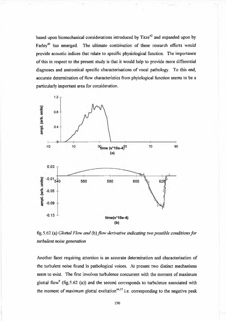
based upon biomechanical considerations introduced by Titze42 and expanded upon by

Farley43 has emerged. The ultimate combination of these research efforts would

provide acoustic indices that relate to specific physiological function. The importance

o f this in respect to the present study is that it would help to provide more differential

diagnoses and anatomical specific characterisations o f vocal pathology. To this end,

accurate determination o f flow characteristics from phyiological function seems to be a

particularly important area for consideration.

(a)

fig. 5.62 (a) Glottal Flow and (b) flow derivative indicating two possible conditions fo r

turbulent noise generation

Another facet requiring attention is an accurate determination and characterisation of

the turbulent noise found in pathological voices. At present two distinct mechanisms

seem to exist. The first involves turbulence concurrent with the moment o f maximum

glottal flow9 (fig.5.62 (a)) and the second corresponds to turbulence associated with

the moment o f maximum glottal excitation44,37 i.e. corresponding to the negative peak

190

in the flow derivative (fig. 5.62 (b)). de Krom37 states that “the energy of turbulent

noise is inversely proportional to the cross sectional area o f the glottal slit”, while

Stevens9 reports “the amplitude of the turbulent noise at the glottis is expected to

increase approximately in proportion to Ag0'5, where Ag is the average glottal area

during a cycle o f vibration”. This apparent contradiction is readily explained by

considering the Reynolds number (eqtn.1.1), where a reduced glottal width or

increased airflow (and corresponding increase in glottal width) can give rise to

turbulent flow. Imaizumi45 has observed turbulent noise both characteristics using a

comb filtering technique46 to extract the noise component. Yet another condition for

turbulent flow is satisfied for patients containing mass lesions or nodules.

The development o f alternative ratios to the traditional harmonic to noise ratio merits

further study requiring more refined ratios and accurate perceptual determinations in

order to provide correct correlations. The perceptual examination o f the patient and

normal data set for the present study (Table.2 .3), rated all patients as dysphonic

(degree not specified) and all the ‘normal’ group were rated ‘normal’ except for two

who showed mild hoarseness and breathiness. Therefore, in the absence of a graded

scale the measure could not be accurately assessed. However, in consideration o f the

fact that the geometric dB mean consistently showed good separability o f the

patient/normal data set we suggest that the ratio shows much promise and that further

research is definitely merited. Similar arguments hold true for the source related ratio,

requiring correlation to accurately determined physical data such as EEG or

stroboscopy ratings. We quote Rothenberg33 on the need for such measures:

“In general there are two types of purposes, namely, to measure or explicate the physiological basis of

the voice characteristics (often the physician’s goal) or to measure or explicate the perceptual

characteristics of the voice (often the therapist’s goal). For example if the vibratory characteristics of

the vocal folds were of interest, a measure emphasising the periodicity in the fundamental frequency

and lower partials might be of interest. If, on the other hand, the perceived pitch were of primary

interest, the periodicity in the energy near the first formant might be a better measure.”

Finally, although a total o f nine separate methods were examined for determining

the harmonic to noise ratio this list is by no means exhaustive. Other methods have

been proposed by the following authors: Ladefoged34 (time domain), Milenkovic47

191

(time domain-comb filter), Imaizumi46 (time domain-comb filter (see appendix A for

source code )), Kasuya (periodicity model)48, deKrom37 (cepstrum), Qi49 (wavelet)

and Gavidia-Ceballos50 The best strategy for introducing new methods is to have a

specific goal in mind. The motivation for each of the three methods introduced here

followed from independent objectives. The two cycle analysis was introduced in

order to spectrally characterise perturbation, the periodogram method was

introduced to motivate the idea o f a noise signal characterising a system and the

possibility o f source derived ratios (as well as providing more consistent spectral

estimates). The pitch synchronous harmonic analysis approach was developed in

order to provide a jitter ( and shimmer) free measurement of the harmonic to noise

ratio. It is hoped that these techniques, particularly the later, will prove

complimentary to the research efforts o f others e.g. Hanson51, Holmberg52,

deKrom53 who have begun to take more diverse spectral measurements from the

acoustic spectra. It is suggested that the ‘long term harmonic spectrum’ (hj(Av)-

eqtn.5.51) may provide more accurate HI (amplitude of first harmonic) to H2

(amplitude o f second harmonic) ratios.

To surmise,

1. A general definition o f noise has been discussed.

2. The spectral properties o f random jitter, cyclic jitter, shimmer and additive

noise have been characterised based on Fourier series, Fourier transform and

periodogram estimation.

3. The harmonic to noise ratio o f the output radiated speech waveform has

been related to the harmonic to noise ratio o f the source.

4. New ratios have been proposed and tested that relate more specifically to

source and perceptual information regarding the voice.

5. Six presently available methods for determining the harmonic to noise ratio

have been successfully programmed and tested with many alterations

introduced.

6. Three new methods for determining the harmonic to nose ratio have been

introduced, namely, periodogram averaging, two cycle analysis and pitch

synchronous harmonic analysis.

192

7. Each new method was developed with a particular emphasis in mind.

Two Cycle - to examine the spectral characteristics o f perturbation.

Periodogram - to show how random noise can be used to characterise a

system.

Pitch Synchronous Harmonic Analysis - to provide a jitter and shimmer free

estimate o f the harmonic to noise ratio.

8. The results from all (except two) o f the analysis techniques show that jitter

and shimmer are included in H/N ratio measurements. The modified

Yumoto approach and the specifically developed pitch synchronous

harmonic approach (psha) showed considerable less sensitivity to the jitter

and shimmer artifacts. The ‘psha’ method was jitter and shimmer insensitive

for the source data.

9. The ‘psha’ approach showed a lot o f promise and many possible

developments were suggested. The technique is complementary to similar

methodologies employed by Fant et al.

10. The results o f the various analyses show that presently used H/N ratios are

useful in determining abnormal voice, especially if the H/N ratio is

bandlimited.

11. The variation o f the H/N ratio for the synthesis data with fO for three levels

of additive noise has been explained. The use o f harmonic number as

opposed to frequency location seems to be merited for studying source

characteristics.

12. Quantitative spectral measurements have been proposed based on the

spectral characterisation results.

13. Future research directions have been considered.

193

5.7 Bibliography

1. Hillenbrand, J. A methodological study o f perturbation and additive noise in

synthetically generated voice signals. J. Speech and Hear. Res. 1987; 30: 448-461

2. Bielamovicz, S. Comparison o f voice analysis systems for perturbation

measurement. J. Speech Hear. Res. 1996; 39: 126-134

3. Yanaghihara, Significance o f harmonic changes and noise components in

hoarseness. J. Speech Hear. Res. 1967; 10:531-541

4. Martin, D. et al Pathological voice type and the acoustic prediction o f severity. J.

Speech Hear. Res. 1995; 38: 765-771

5. Pruszewicz, A. et al Usefulness o f acoustic studies on the differential diagnostics o f

organic and functional dysphonia. Acta. Otolaryngol. 1991; 111: 414-419

6. Valencia-Naranjo, N. et al Diagnostic voice disorders. Current opinion in head and

neck surgery 1995 3: 164-168

7. Titze, IR. Towards standards in acoustic analysis o f voice. NY: Raven Press J.

Voice 1994; 8: 1-7

8. Rontal, E. et al Objective evaluation o f vocal pathology using voice spectrography.

Ann. Otol. 1975; 84: 662-671

9. Stevens, KN. Airflow and turbulent noise for fricative and stop consonants , J.

Acoust. Soc. Am. 50:1180:1192

10. Muta, H. et al Analysis o f hoarse voices using the LPC method. Laryngeal

function in phonation and respiration. Boston : Little Brown, 1987 pp. 463-474

11. Titze, IR. and Liang. H. Comparison o f ft) extraction methods for high precision

voice perturbation measurements. 1993; 36: 1120-1133

12. Harris, FJ. On the use o f windows for harmonic analysis with the discrete Fourier

transform, Proc. o f the IEEE, 1978 66:51:142

13. Blackman, RB. and Tukey, JW. The measurement o f power spectra. Toronto,

Ontario: General Publ. Company, 1959

14. Klingholtz, M. and Martin, F. Quantitative spectral evaluation o f shimmer and

jitter. J. Speech Hear. Res. 1985; 28: 169-174

194

15. Gauffin, J. et al Irregularities in the voice: A perceptual experiment using synthetic

voices with subharmonics. In PJ Davis and NH. Fletcher (Eds.) Controlling

complexity and chaos. San Diego: Singular Publ. Co., 1996

16. Fant, G. Acoustic theory o f speech production. Mouton, The Hague, 1970.

17. Deller JR. et al Discrete time processing o f speech signals, New York:Macmillan,

1993

18. Fant, G. and Lin, Q. Frequency domain interpretation and derivation o f glottal flow

parameters. STL-QPSR 1988, 2-3:1-23

19. Kitajima, K. Quantative evaluation o f the noise level in the pathologic voice. Folia

phoniat. 1981; 33: 115-124

20. Hiraoka, N. et al Harmonic intensity analysis of normal and hoarse voices. J.

Acoust. Soc. Am. 1984; 76: 1648-1651

21. Oppenheim AV. and Schafer RW. Discrete-time signal processing. Englewood

Cliffs, N.J.: Prentice Hall, 1989

22. Jenkins, GM. and Watts DG. Spectral analysis and it’s applications. San Francisco:

Holden-Day, 1968

23. Kasuya, H. et al Normalised noise energy as an acoustic measure to evaluate

pathologic voice. J. Acoust. Soc. Am. 80: 1329-1334

24. Muta, et al A pitch synchronous analysis o f hoarseness in running speech. J.

Acoust. Soc. Am. 1988; 84: 1292-1301

25. Kojima, H. et al Computer analysis o f hoarseness. Acta. Otolaryngol. 1980; 89:

547-554

26. Yumoto, E. et al Harmonic-to-noise ratio as an index o f the degree o f hoarseness.

J. Acoust. Soc. Am. 71: 1544-1549

27. Hammarberg, B. and Gauffin, J. Perceptual and acoustic characteristics o f quality

differences in pathological voices as related to physiological aspects. In O. Fujimura

and M. Hirano (Eds.) Vocal fold physiology: Voice quality control, 1995

28. Rabiner L. and Schafer R. Digital processing o f speech signals. Englewood Cliffs,

N.J.: Prentice Hall, 1978

29. Fant, G. and Lin, Q. Frequency domain interpretation and derivation o f glottal flow

parameters. STL-QPSR 1988, 2-3:1-23

195

30. Imaizumi, S. et al Harmonic analysis o f the singing voice: - Acoustic

characteristics o f vibrato. Proc. o f the Stockholm Music Acoustics Conference,

Stockholm, (SMAC 93)

31. Horii, Y. Fundamental frequency perturbation observed in sustained phonation. J.

Speech and Hearing Res. 1979; 18: 19-201

32. Mathews, MV. et al Pitch synchronous analysis o f voiced sounds. J. Acoust. Soc.

Am. 1971; 33: 179-186

33. Rothenberg, M. In O. Fujimura (Ed.) Vocal fold physiology: Voice production,

mechanisms and functions. NY: Raven Press, 1988

34. Ladefoged, P. In O. Fujimura (Ed.) Vocal fold physiology: Voice production,

mechanisms and functions. NY: Raven Press, 1988

35. Koike, Y. and Kohda, J. The effect o f vocal fold surgery on the speech cepstrum.

In J. Gaufin and B. Hammarberg (Eds.) Vocal fold physiology: Acoustic, perceptual

and physiologic aspects o f voice mechanisms. San Diego : Singular Publ. 1991

36. Titze, IR. Three models of phonation. J. Acoust. Soc. Am. Suppl. 1 79: S81

37. de Krom, G. A cepstrum based technique for determining a harmonics-to-noise

ratio in speech signals. J. Speech Hear Res. 1993; 36: 254-266

38. Kasuya, H. and Endo, Y. Analysis, synthesis and perception o f brathy voice. InJ.

Gaufin and B. Hammarberg (Eds.) Vocal fold physiology: Acoustic, perceptual and

physiologic aspects o f voice mechanisms. San Diego: Singular Publ. 1991

39. Fujimura, O. In O. Fujimura (Ed.) Vocal fold physiology: Voice production,

mechanisms and functions. NY: Raven Press, 1988

40. Gobi, C. Voice source dynamics in connected speech. STL-QPSR 1:123-159

(Dept, o f Speech Communication and Music Acoustics, Royal Institute of

Technology, Stockholm).

41. Karlsson, I. Glottal waveform parameters for different speaker types. Proc.

SPEECH ’ 88 (7thFASE Symp.), 1:225-231. (Institute of Acoustics, Edinburgh).

42. Titze, IR. Mechanisms underlying the control o f fundamental frequency. In J.

Gaufin and B. Hammarberg (Eds.) Vocal fold physiology: Acoustic, perceptual and

physiologic aspects o f voice mechanisms. San Diego: Singular Publ. 1991

43. Farley, GR. A biomechanical laryngeal model o f voice fO control and glottal width

control. J. Acoust. Soc. Amer. 1996,100:3794-3812

196

44. Lee, CK. Childers, DG. Some acoustical, perceptual and physiological aspects o f

vocal quality. In J. Gaufin and B. Hammarberg (Eds.) Vocal fold physiology:

Acoustic, perceptual and physiologic aspects o f voice mechanisms. San Diego:

Singular Publ. 1991

45. Imaizumi, S. A preliminary study on the generation of pathological voice qualities.

In 0 . Fujimura (Ed.) Vocal fold physiology: Voice production, mechanisms and

functions. NY: Raven Press, 1988

46. Gauffin, J. et al, S. A microcomputer based system for acoustic analysis o f voice

characteristics. ICAPP 1986 IEEE 677-684

47. Milenkovic, P. et al Acoustic and perceptual characterisation o f vocal nodules. In J.

Gaufin and B. Hammarberg (Eds.) Vocal fold physiology: Acoustic, perceptual and

physiologic aspects o f voice mechanisms. San Diego: Singular Publ. 1991

48. Kasuya, H. and Endo, Y. Acoustic analysis, conversion and synthesis o f the

pathological voice. In O. Fujimura and M. Hirano (Eds.) Vocal fold physiology:

Voice quality control, San Diego: Singular Publ., 1995

49. Qi, Y. Time normalisation in voice analysis. J. Acoust. Soc. Am. 1992; 92: 1569-

76

50. Gavidia-Ceballos L. Hansen JH. Direct speech feature estimation using an iterative

EM algorithm for vocal fold pathology detection. IEEE Trans, on Biomedical Eng.

1996; 43: 373-83

51. Hanson, HM. Glottal characteristics o f female speakers; Acoustic correlates. J.

Acoust. Soc. Am. 1997; 101:466:481

52. Holmberg, EB. Comparisons among aerodynamic, electroglottographic and

acoustic spectral measures o f female voice. J. Speech Hearing Res. 1995,

38:1212:1223

53. de Krom, G. Some spectral correlates o f pathological breathy and rough voice

quality for different types o f vowel fragments. J. Speech Hear. Res. 1995; 38: 794-

811

197

Chapter 6

Long Term Average Spectrum Analysis

6.1 Introduction

The long term average spectrum (LTAS) is defined as the ensemble average o f

successive spectral estimates for a given sample o f speech. The speech material in this

case might typically consist o f reading a paragraph o f newspaper text. The use o f

LTAS derived measures has been the primary method o f choice for speaker verification

systems for some time now1,2. Part o f their attraction is that they offer the possibility o f

text independent measurements o f speaker identifying features i.e. if a sufficiently long

sample o f speech is taken, the resulting averaged spectrum contains information

pertinent to speaker identification as opposed to the words spoken.

The LTAS has also been well documented in the speech pathology literature although

opinions on it’s potential use as an objective indicator o f dysphonia have been

divided.3’4 Hammerberg et al5 successfully used the LTAS to differentiate breathiness

conditions o f both hypofimction and hyperfunctional voice. Wendler also found it to

be a very promising measure but later tailored his initial optimistic opinions on it’s use6.

198

In a study performed by Lofqvist7 (1986) an attempt was made to differentiate a set o f

37 clinical voices from a set o f 36 normal voices. The two measures taken from the

LTAS were the ratio o f the energy below 1 kHz to the energy from 1 to 5 kHz and the

energy level between 5 and 8 kHz. The result o f the analysis produced almost a

complete overlap o f patient and normal data and Lofqvist therefore expressed a

pessimistic view for it’s use in clinical investigations. In another study by Lofqvist8 he

states that, in applying the LTAS

“... the short term variations due to phonetic structure will be averaged out and the resulting spectrum can be used to obtain information on the sound source: if the analysis is restricted to voiced sounds, the sound source is the vibrating glottis.”

He therefore felt that the two LTAS derived measures were indicative o f the sound

source. He also investigated the effect o f the time length on the LTAS and noticed that

reducing a sample o f voiced speech from 20 to 10 seconds had little effect, however,

further reduction in the sample length made the LTAS variations unpredictable. In a

study performed by Kitzing9 at the same time as the Lofqvist work, an extensive set of

LTAS derived measured were investigated. Their measures in particular proved useful

for separating strained and sonorous vocal qualities: ( 1) the ratio o f energy below and

above 1 kHz , 2) a measure o f the spectral slope inclination in the first formant range

and (3) the ratio o f the peak level o f the fundamental and the first formant region. In a

later study10 he found that LTAS derived measures correlated moderately well with

perceived improvements in patients undergoing voice therapy.

6.2 Analysis

As stated above, LTAS is generally used on connected speech where the vocal tract

filter function varies with time. Advantages11 and disadvantages12 o f using connected

speech have both been reported in the speech pathology literature. From the point of

view of general speech disorders or disorders associated with articulatory dynamics

connected speech is the preferred choice. An obvious example would be spasmodic

199

dysphonia13, where the aberrant vocal quality might not show up during the phonation

of a sustained vowel but is easily detected in running speech.

Although a phonetically balanced sentence o f about 2 seconds duration was recorded

for all patients in this study and a program was successfully coded (thres.m - appendix

x) to remove unvoiced segments of speech based on amplitude and zero-crossing rate

considerations, it was decided not to use connected speech for the following reasons:

1. Lofqvist7 reported variable LTAS results if the speech sample used was less

than 10 seconds.

2. The result o f a study by Anathapadmanabha15 (1992), based on LTAS derived

from a two second sample o f connected speech showed LTAS to be a poor

indicator o f vocal quality.

3. We do not agree with Lofqvist’s assumption that averaging a sufficient

number of spectra will cancel the overall formant contributions and therefore

leave a spectrum directed related to the voice source. This would require that

the sum o f the vocal tract spectra (second term of the third expression in

eqtn.6 .1) would add to zero.

LTAS(f) = Si(f) = £ Ei(f) x V;(f) = E(f) x £ V,(f) eqtn.6.1^ i= l i= l i= l

Ei = i* source spectrum

Vi = Ith vocal tract spectrum

Si = i* speech spectrum

Where it is assumed that E;(f) is constant.

Therefore measures o f fundamental frequency (fO) and first formant (fl) levels taken

from the LTAS should be treated with caution in respect to how they relate to the

voice source. Or as pointed out by Kitzing10,

200

even if it may be possible to neutralise the influence of isolated vowel articulation by averaging a sufficient number of spectra, there is always still a substantial influence from articulation and the resonators of the vocal tract on the spectrum.”

A sustained phonation o f the vowel a/ is used in the analysis. This was felt to represent

the voice source more directly, even though the influence o f the vocal tract resonating

cavities are o f course present in order to produce the vowel resonances, the

configuration is fixed and therefore the spectra do not add in an unpredictable manner.

Averaging several short time spectra across a given phonation reduces the variance o f

the spectral estimates which can be quite high for non deterministic or random signals.

This so called periodogram15 averaging was thought useful in anticipation o f the

aperiodicities and random noise found in pathological voices.

The program ltas.m was coded in the Matlab high level language with the following

input parameters.

1. window size 256

2 . hop size 100

3. total length 0.75 sec

Another version (ltashfe.m) o f the program was also written in order to provide high

frequency emphasis in the spectrum. The source code is given in appendix A. The

LTAS for two normals and two patients o f the present study are shown in fig.6 .1.

Four measures were taken from the resultant spectra :

1. The ratio o f the energy below 1 kHz to that above 1kHz. (Ri4)

2. The ratio o f the energy below 2 kHz to that above 2kHz. (R24)

3. The ratio o f the energy below 1 kHz to that above 1kHz taken from a dB-averaged

spectra.

4. The ratio o f the energy below 2 kHz to that above 2kHz taken from dB-averaged

spectra.

Where R14 and R24 were calculated form the following equations

201

ampi

. (d

B)

— i------------------- 1--------------------1------------------- 1------------------- 11000 2000 3000 4000 5000

frequency (Hz)(a)

1 0 0 0 2000 3000f r e q u e n c y ( H z )

(b)

4000 5000

f r e q u e n c y ( H z ) ( c )

f r e q u e n c y ( H z )

(d)

fig.6.1 LTAS fo r (a), (b) two ‘normals ’ and (c), (d) two patients o f the present study

with window length 25.6 ms, hop size 10 ms and total analysis length 0.75

second

N / 5

X A .-R 14 = 5 x N / 4 eqtn.6.2

i= N IS

N x 2/5

R 24 = eqtn.6.3

i= N X 2/5

where Ai is the spectral amplitude at the i* frequency

location taken from the LTAS.

N = number o f spectral estimates o f the LTAS (128) covering up to 5 kHz.

6.3 Results

The above program was run on all the synthesis data files detailed in table 2.5 o f

chapter 2. LTAS are show for the four different perturbation measures in fig.6 .2. The

results for (1) and (2) above are given in fig.6.3 and fig.6.4 for the 110 Hz synthesis of

the vowel a/. As can be seen in the figure, as the additive noise level increases the Ru

and R24 ratios decrease. As the noise is mean zero, Gaussian noise it has a flat spectral

characteristic. In considering the source spectrum, equal amounts o f energy are added

to the signal but because the lower partials o f the source are significantly greater in

magnitude the influence o f the additional noise has a much lesser effect on the

numerator in eqtn.6.2 and eqtn.6.3 than it has on the denominator. The magnitude o f

the resonant contributions o f the vocal tract are also a consideration. The results for

the jitter set signals and the shimmer signals are shown in fig. 6.5 and 6.6 respectively.

An examination o f these graphs reveals that the Rw and R24 ratios are somewhat

insensitive to jitter and shimmer and even for the maximum amounts o f jitter and

shimmer added, the ratios are above the corresponding ratios obtained for the additive

noise signals.

203

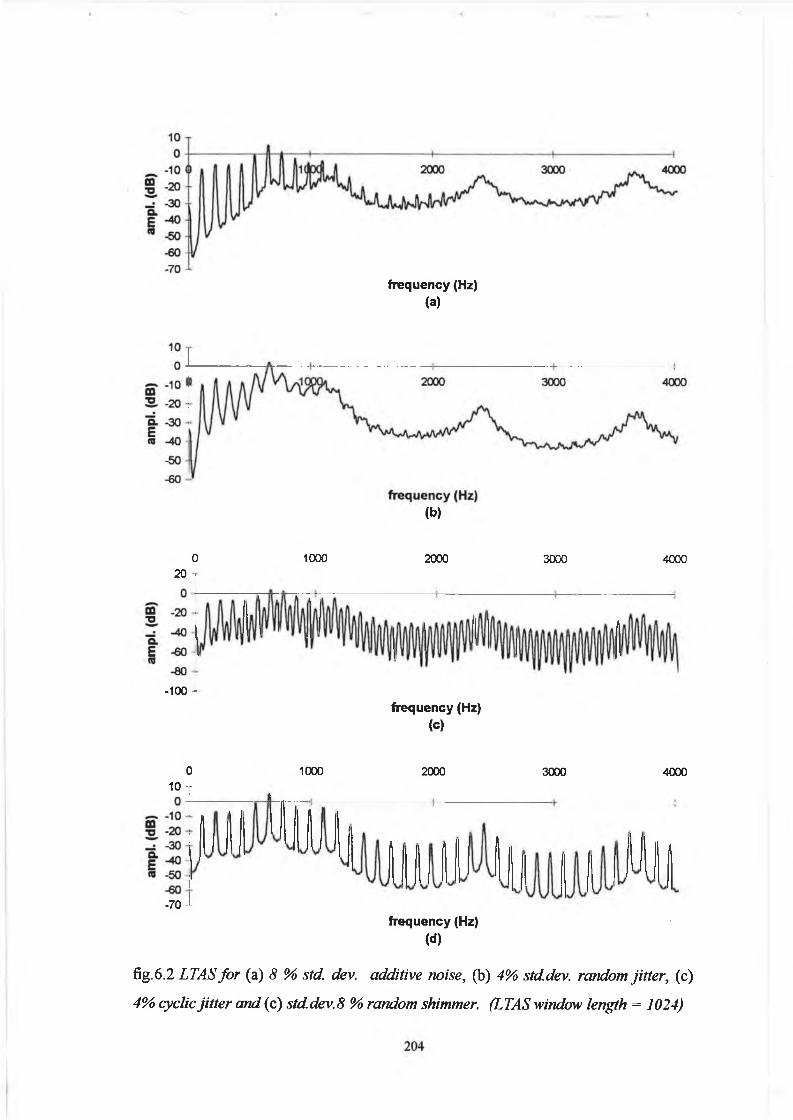
frequency (Hz) (a)

(b)

0 1000 2000 3000 400020 r

-100 1frequency (Hz)

(c)

0 1000 2000 3000 400010 T

-70-*•frequency (Hz)

(d)

fig.6.2 LTAS for (a) 8 % std. dev. additive noise, (b) 4% stddev. random jitter, (c)

4% cyclic jitter and (c) stddev. 8 % random shimmer. (LTAS window length = 1024)

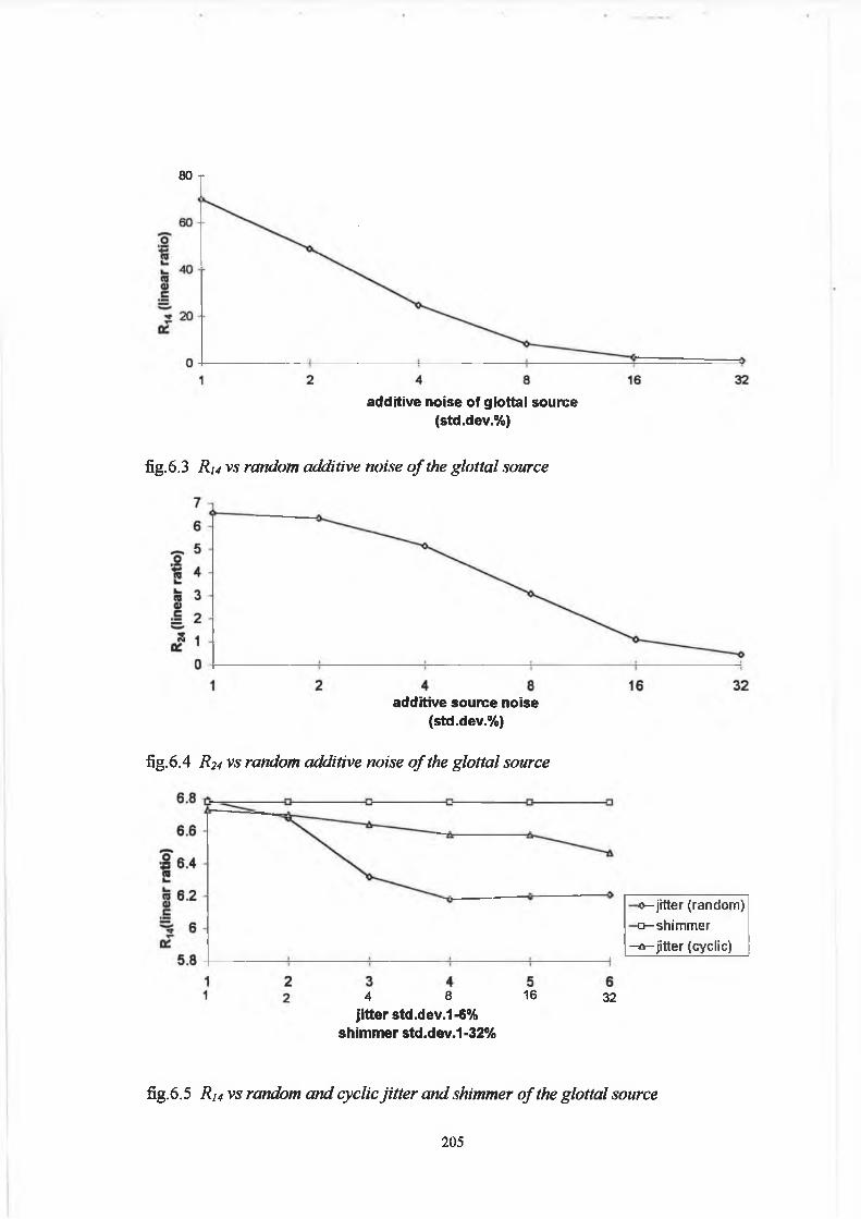
80 r

additive noise of glottal source (std.dev.%)

fig.6.3 Ri4 vs random additive noise o f the glottal source

additive source noise (std.dev.%)

fig.6 .4 R24 vs random additive noise o f the glottal source

4 8

jitter std.dev.1 -6% shimmer std.dev.1 -32%

16

o-jitte r (random) q - shimmer

-a - jit te r (cyclic)

32

fig.6.5 R14 vs random and cyclic jitter and shimmer o f the glottal source

205

(0g 84

—o—jitter (random) -a -sh im m er - a- jitter (cyclic)

762

243

84

165

326

jitter std.dev.1-6% shimmer std.dev.1-32%

fig. 6.6 R.24 v s random and cyclic jitter and shimmer o f the glottal source

This is an interesting result in that we now have a ratio that is representative o f additive

noise and independent o f jitter and shimmer values. Although, of course we should

keep in mind that this result is critically dependent on how well we have modelled the

noise signal. The results obtained for (3) and (4) above proved inconclusive and were

not considered further as were the results from the high frequency emphasis program.

The ltas.m program was next run on the patient/normal data files for the vowel a/.

Histograms o f the results is given in fig.6.7 and fig.6.8. Referring to these figures, it

can be seen that the R24 ratio shows poor separability, whereas the R14 ratio has

separated all but one o f the patients from the normal data. Interestingly, however the

results are in complete opposition to the ratios obtained with the additive noise (fig.

6.2). In respect to the RJ4 ratio, the ‘normal’ data are in agreement with values

obtained from the low additive noise or perturbation results whereas the patient data

shows a marked increase in this ratio. Firstly, it is encouraging that the ratio, which

was shown to reflect additive noise levels, independent o f jitter and shimmer, has

separated the real data. However, it also raises questions about our simplistic model

for simulating pathologies. In our model the glottal waveform maintains it’s shape

with the open and closed periods remaining fixed and signal dependent, mean zero,

Gaussian noise is introduced. In this manner no noise is added during the closed phase

as the airflow is assumed to be zero during this period. In more realistic models o f

glottal flow we would expect the closed phase to be less pronounced in many cases

206

5 t

0 4 B 12 16 20 24 28 32 36

Energy Ratio R14 (0-1/1 -4kHz) (linear ratio)

fig.6 .7 Histogram o f Ri 4 fo r the patient/normal data set. Highly significant at the 5

% level (one tailed\ two sample, equal variance, student ’s t-test).

10 15 20 25 30 35 40

Energy Ratio RM (0-2/2-4kHz) (linear ratio)

fig.6.8 Histogram o f R24 fo r the patient/normal data set. Not significant a t the 5 %

level (one tailed, two sample, equal variance, student’s t-test)

involving voice pathologies. This might be due, for example, to the effect o f mass

lesions such as nodules, polyps etc. which would result in appreciable airflow leakage

even when the vocal processes come into contact during the attempted close phase of

the cycle. Incomplete or reduced closed phase also occurs in hypofunctional and

breathy voices or as a result o f vocal cord paralysis or paresis. The acoustic effect o f

this, is a reduction in harmonic structure in the higher frequency end o f the spectrum

which leads to an overall reduction in energy in the upper part of the spectrum despite

207

having an increase in noise energy in this region. Also, the lower frequency region may

have an increase in the lower frequency components due to the more sinusoidal nature

o f the glottal flow waveform. The overall result o f this is an increase in the R14 ratio

(also referred to as called spectral tilt).

6.4 Discussion and Conclusion:

The LTAS has been obtained from sustained phonations rather than from connected

speech for the reasons outlined in section 6.2. Averaging (n) the spectrum o f a

sustained phonation reduces the variance o f the spectral estimates by 1/n at the expense

o f broader bandwidths and hence reduced resolution. Two measures, the ratio o f the

energy below 1 kHz to the energy above 1 kHz (Ri4) and the ratio o f the energy below

2 kHz to the energy above 2 kHz (R24) were considered for analysis. Both the R i4 and

R24 ratios decreased with increasing levels of additive noise. Both methods were also

relatively insensitive to jitter and shimmer. Furthermore, R14 has been shown to be a

useful indicator o f vocal pathology.

A number of studies have attempted to relate the spectral effects of varying parameters

in the glottal flow waveform. Most o f this work is based on Fant’s four parameter LF-

model o f glottal flow16 (fig. 6 .8) where the four parameters are derived from the three

basic time events that occur during the glottal cycle, 1) the location o f peak flow, Tp 2)

the discontinuity point at glottal closure, Te and 3) the return phase, Ta. In relation to

the source spectrum, these studies have revealed that:

1) the level o f the fundamental is closely related to the rising portion o f the flow

glottogram.

2) the rate o f closure corresponds to the level o f all upper partials, i.e. a higher

closing speed gives rise to an increase to all higher harmonics.

3) the spectral tilt is very dependent on the final part o f the closing phase that

appears after the instant o f maximum airflow decrease.

208

fig. 6.8 Four parameter model o f differentiated glottal flow illustrating the three main

time events that occur during the glottal cycle - 1) the location ofpeak flow, Tp 2) the

discontinuity point at glottal closure, Te and 3) the return phase, T&

The Ri4 measure incorporates all o f these source spectrum characteristics. Therefore

to investigate the measures independently, other spectral measurements are required.

The ratio o f the amplitude o f the first harmonic to the amplitude o f the second

harmonic is thought to relate to abductory behaviour17 whereas the ratio o f the

amplitude o f the first harmonic to the amplitude of the third formant is thought to

relate more closely to the closing phase18,19. In our glottal flow waveform, adductory

and abductory behaviour were purposely not altered in order to firstly examine the

gross spectral characteristics o f jitter, shimmer and additive noise. There are obvious

advantages o f modelling in this fashion, in that there is a strict control on the variables,

a situation always absent, even for ‘normal’ voice. The disadvantage is that these

situations may, in fact, not be physically realisable. Independent model parameters may

not behave in an unconstrained manner in practical situations. Gauffin and Sundberg20

made a similar comment when comparing the flow glottograms o f singers and non-

singers:

“As the Fant model is theoretical, it will consider cases, regardless of whether or not they occur

in reality. In our material on the other hand, we have included only normal or trained voices.

In pathological voices, glottogram characteristics may be combined in other ways”.

So, in detailing the spectrum in respect to it’s ability to extract salient cues to vocal

pathology we must consider, a) the spectral consequences o f the variable parameters

that occur in the four parameter model and b) the spectral consequences o f additional

features important to vocal pathology. Additional factors for consideration (to those

mentioned above) include the type o f phonation, such as soft, normal and loud and in

respect to the spectral analysis, how many frames to average, overlap etc. or whether

and when to use a pitch synchronous harmonic analysis.

As previously mentioned, use o f the LTAS on short segments o f speech, has not been

very successful in making correlations with vocal qualities14. An interesting alternative

to using the LTAS, would be to investigate the long term harmonic spectrum, LTHS,

defined as the ensemble average o f successive harmonic estimates for a given sample of

speech i.e. spectra are extracted pitch synchronously and subsequently averaged

according to harmonic number as opposed to frequency location. Alternatively, pitch

synchronous inverse filtering, based on a spectral matching procedure, followed by

averaging facilitates a more direct comparison to the parameters included in the LF

model o f glottal flow.

A further advantage o f making calculations based on harmonic number as opposed to

frequency location is that the ratio o f the number o f harmonics within the 0-1 kHz

range to the 1-4 kHz range changes with fundamental frequency. Table 6.1 illustrates

these ratios for the synthesis data files. Using harmonic numbers the ratio is o f course

constant. An obvious objection to this approach is that the harmonics receive different

resonant contributions if the fundamental frequency is different. A possible solution

would be to calculate the ratio between harmonic to noise ratio from 0-1 kHz to the

harmonic to noise ratio from 1-4 kHz. Another factor for consideration is the

relationship between the harmonic locations in relation to the position o f the formant

peaks. Figure 6.8 (a) and (b) show how the R14 and R24 ratios vary with fundamental

frequencies. The fact that the harmonics in the spectrum of the low fundamental

frequency data file have attenuated by 2 kHz and the harmonics for the higher

fundamental frequency data are still very prominent at 5 IcHz is also an important

consideration.

Finally, basic research is required in order to relate glottal flow (and hence spectral)

characteristics to specific vocal pathologies o f aberrant vocal fold vibrations. The

210

Vowel a/ with first three resonances at -660, ~ 1 100 and -2400 Hz

fundamental

frequency /

number o f

harmonics

80 110 160 220 290 350

a) 0-1 kHz 12 9 6 4 3 2

b) 1-4 kHz 38 27 19 14 10 9

ratio a) / b) 0.316 0.333 0.316 0.286 0.3 0.22

Table.6 .1 Ratio o f number o f harmonics from 0-1 kHz to number o f harmonics to 1-4

kHz.

160 TO (Hz) 220 (a)

— o— noise 4 —a— noise 8 — a — noise 16

fig.6.9 Variation o f (a) R j4 and (b) R24 with fundamental frequency fo r three levels o f

additive random noise o f std. dev. 4, 8 and 16% .

211

connection between flow characteristics is not always obvious and this link in the

speech chain may prove to be the limiting factor in the potential usefulness o f acoustic

analyses with regard to differential and accurate diagnoses o f varying pathology types.

A couple o f examples o f possible inferences based on flow characteristics are given.

From a knowledge o f the rate o f decrease o f airflow before closure we may be able to

infer how the closure occurred along the length o f the vocal process, beginning

anteriorly and continuing until the posterior processes approximate (if they do).

Subsequent to this is the closed phase. The length of this period after a given rate of

decrease o f volume velocity might provide information regarding the tissue properties

of the folds (elasticity and impact stress). The next example helps illustrate the possible

ambiguities that could possibly arise from inferences regarding vibratory characteristics

based on the flow characteristics. When assymmetry of phase occurs, the vocal fold

consistently move in the same direction (Diane Bless21 illustrates a nice example on her

instructional stroboscopy video cassette). This results in a constant glottal area with

no open or closed phase. Greater airflow with possible turbulent characteristics

therefore results. It remains to be seen if the acoustic analyses including LTAS and

associated parameters can differentiate the resultant airflow characteristics from this

type o f dysfunction with turbulent flow due to the presence of polyps or mass lesions.

Hence the need for basic research correlating acoustic analysis parameters to

alternatively assessed specific pathology types.

212

1. Rosenberg, AE. Automatic speech verification : a review, Proc. IEEE 1976; 64:

475-487

2. Hollien, H. et al Speaker identification by long term spectra under normal, stess and

disguised conditions. J. Acoust. Soc. Am. 1974; 55: S-20(A)

3.Wendler, J. et al: Voice calssification by means o f long term spectra. Folia Phoniat.

1980 32: 51-60

4. Prytz, Long time average spectra (LTAS) of normal and pathological voices; Proc.

17th Int. Congr. Logopedics Phoniat. 1977; 1: 459-475

5. Hammarberg, B. et al erceptual and acoustic correlates of abnormal voice qualities.

Acta. Oto-lar. 1980; 90: 441-451

6. Wendler, J. et al, Classification o f voice qualities. Journal of Phonetics 1986 14:

483-488

7. Lofqvist, A. Mandersson, B. Long-Time Average Spectrum of Speech and Voice

Analysis Folia phoniat. 1987; 39: 221-229

8. Lofqvist, A. The Long Time Average Spectrum as a tool in voice research, J.

Phonetics 1986; 14: 471-475

9. Kitzing, P. LTAS criteria pertinent to the measurement of voice quality. J.

Phonetics 1986; 14: 477-482

10. Kitzing, P. and Akerlund, L. Long time average spectrograms o f dysphonic voices

before and after therapy. Folia Phoniatr. 1993; 45:53-61

11. Pruszewicz, A. et al Usefulness o f acoustic studies on the differential diagnostics

of organic and functional dysphonia. Acta. Otolaryngol. 1991; 111 : 414-419

12. Fex, B. Acoustic analysis o f functional dysphonia: before and after voice therapy

(accent method) J. Voice 1995 8: 163-167

13. Blitzer, A. et al Clinical and laboratory characteristics o f focal laryngeal dystonia:

study o f 110 cases. Laryngoscope 1988; 98: 636-640

14. Ananthapadmanabha, TV. Acoustic factors determining perceived voice quality. In

O. Fujimura and M. Hirano (Eds.) Vocal fold physiology: Voice quality control, San

Diego: Singular Publ., 1995

6.5 Bibliography

213

15. Rabiner, L. and Schafer, R. Digitial processing o f speech signals, Englewood Cliffs,

N.J.: Prentice Hall, 1978

16. Fant, G. and Lin, Q. Frequency domain interpretation and derivation of glottal flow

parameters. STL-QPSR 1988, 2-3:1-23

17. Klatt, DH. and Klatt, LC. Analysis, synthesis and perception o f voice quality

variations among female and male talkers. J. Acoust. Soc. Am. 1990; 87: 820-857

18. Holmberg, EB. Comparisons among aerodynamic, electroglottographic and

acoustic spectral measures o f female voice. J. Speech Hearing Res. 1995,

38:1212:1223

19. Hanson, HM. Glottal characteristics o f female speakers; Acoustic correlates. J.

Acoust. Soc. Am. 1997; 101:466:481

20. Gauffin, J. and Sundberg, J. Spectral correlates o f glottal source waveform

characteristics. J. Speech Hear. Res. 1989; 32: 56-565

21. Bless, D. et al Comparison o f vibratory characteristics o f young adult males and

females. In M. Hirano and R. Hibi (Eds.) Proc. o f the Int. Conf. on Voice. Kurume,

Japan. 1986;2:46-54

214

Chapter 7

Cepstral Analysis Techniques

7.1 Introduction

The term cepstrum first appeared in the scientific literature in a paper with the unusual

title: ‘The Quefrency Alanysis o f Time Series for Echos: Cepstrum,

Pseudoautocovariance, Cross-Cepstrum, and Saphe Cracking”1. The paper was

published in 1963 by Bogert, Healy and Tukey in which they observed that the

logarithm o f the power spectrum o f a signal containing an echo has an additive periodic

component due to the echo, and thus the Fourier transform of the logarithm of the

power spectrum should exhibit a peak at the echo delay. They called this function the

‘cepstrum’, reversing the order o f the first four letters in the word spectrum because

according to Bogert et al “we find ourselves operating on the frequency side in ways

customary on the time side and vice versa.” Tukey went on to liberally define a rich

vocabulary o f terms reflecting the fact that the resultant functions lay neither properly

in the time or frequency domains. However, only the words cepstrum, rahmonics,

quefrency and liftering have found popular usage.

215

The use o f the cepstrum function by the above authors to locate echos in seismic data

was not very successful. Schroeder2 suggested it’s use for analysing speech signals,

given that the log o f the short time spectrum for voiced speech exhibits an envelope

corresponding to the vocal tract transfer function with a superimposed periodic

component due to the glottal source. The Fourier transform of this spectrum should

therefore lead to a prominent peak corresponding to the pitch period and a large signal

based around zero Hertz reflecting the spectral envelope. The cepstral technique

proved very robust in detecting the pitch period of voiced speech, even in the presence

o f additive noise: a detailed account is given in Noll3. The ability o f the cepstrum to

separate the source and envelope characteristics of the speech was next put to use in

formant extraction schemes4 and more recently cepstral coefficients have replaced LPC

coefficients in advanced speech recognition systems5. Before going on to review

cepstral methods as applied to speech pathology we should note that the cepstrum

comprises one o f several methods that fall under the general heading of

‘Homomorphic Deconvolution’. This new class o f systems was proposed by

Oppenheim6 shortly after the paper by Bogert et al. They are nonlinear systems in a

classical sense but they do follow a type of generalised superposition principle i.e. input

signals and their corresponding responses are superimposed by an operation having the

same algebraic properties as addition.

Despite the above mentioned success o f cepstral methods in speech analysis they have

received very little attention in the vocal pathology literature. A complete review of

the literature reveals only three independent authors to have investigated it’s use as an

indicator o f vocal pathology. Koike7 has used the method on three separate occasions

to assist patient diagnosis. The height o f the first cepstral peak (first rahmonic) was

used as an indicator o f good periodicity and the location o f this peak on the quefrency

axis was used to determine the pitch period. Positive, objective assessment was

reported through using the method and a call for further studies was made.

Hillenbrand8 also calculated the height o f the first cepstral peak, using a normalisation

procedure in which he did not check for pitch tracking errors and yet found the method

very useful in predicting breathiness. By far the most comprehensive assessment o f the

technique with respect to it’s application to speech pathologies was the work by

de Krom9, “A Cepstrum-Based Technique for Determining an Harmonic-to-Noise

216

Ratio in Speech Signals”, in which he removed the rahmonics in the cepstrum, Fourier

transformed the resulting liftered cepstrum to provide a noise spectrum which was

subtracted from the original log spectrum. This resulted in, what we have termed, a

source related spectrum. After performing a baseline correction procedure on this

spectrum, the modified noise spectrum was subtracted from the original log spectrum

in order to provide the harmonic to noise ratio estimate. This work used speech

samples synthesized to simulate various amounts of jitter and additive noise conditions

in a manner similar to the files produced here, de Krom pointed out the absence o f a

database o f pathological voices samples from which researchers might investigate new

analysis techniques and citing the dangers o f using pathological voice samples with

vague assessments suggested the use o f synthetic signals as an objective, quantifiable

alternative. This is the procedure followed throughout this study. In addition to this,

for the cases outlined here, once a method appeared successful based on the synthesis

data, it was then used in an attempt to discriminate between a group of thirteen patients

with various voice disorders (Table.2.1 Chapter 2) and twelve normal speakers. The

method detailed in this chapter is developed along the same lines as the de Krom

technique, but the present procedure follows fewer steps, leading to a source related

harmonic to noise ratio (H/Ns). Hillenbrand’s normalisation scheme and bandlimited

analysis was also tested.

7.2 Method

Noll pointed the way forward towards an easy explanation o f the seemingly

complicated cepstrum technique, stating that “the spectrum itself can be regarded as a

signal and can be processed by standard signal-analysis techniques”. We follow this

intuitive approach to the cepstrum of voiced speech in the outline that follows.

For voiced speech we know that s(t) can be represented as the convolution o f the

excitation signal and the impulse response o f the vocal tract transfer function (fig. 7.1).

217

X(ffl) S(û))

fig. 7 .1 Source/filter model o f speech production illustrating impulse and frequency

responses.

s(t) = x(t)*v(t) eqtn.7.1

s(t) = output radiated speech waveform

x(t) = glottal source

v(t) = transfer function o f the vocal tract

* indicates convolution

This is equivalently represented by the frequency response o f the vocal tract as

S (o )= |X(<d) | x | V (cd) | eqtn.7.2

where S(o) = F(s(t)), X(co) = i 7(x(n)), V(co) = F(v(n))

where F represents Fourier transformation.

Now, by simply taking the logarithm o f the spectrum, we obtain

log|S(<o)| = log| X (o) | x log| V (o) |

log|S(co)| = log[X(co)| + log|Y(o))|

eqtn.7.3

218

Therefore the multiplicative components consisting o f the source excitation (fast

varying) and filter function (slow varying) have been changed into additive

components. The motivation for doing this is that we can now apply a linear operator,

i.e. the Fourier transform, knowing that the transform operates individually on the two

additive components and that the transform will conveniently separate the slowly

varying part from the fast varying part. In this way we are considering the signal

log|S(w)| as a standard “time” signal with one “high frequency” and one “low-

frequency” component, the Fourier transform o f which, gives a high amplitude at

locations in the “frequency domain” corresponding to these frequencies. Since, we

were in the frequency domain to begin with the new terminology (rahmonics,

quefrency, etc.) was employed to reflect this distinction between the resultant and that

which would have occurred with using real time domain signals. This process is

illustrated in fig.7.2. Therefore taking the inverse Fourier transform of the log

magnitude spectrum yields the real cepstrum

C(t)= IDFT[log|S(<o)|] eqtn.7.4

where t represents quefrency

and IDFT is the inverse discrete Fourier transform.

Note the complex cepstrum is obtained by simply replacing the magnitude spectrum,

|S(co)|, with the Fourier spectrum, S(co). The complex cepstrum is rarely used in

practice and is only o f interest where knowledge o f the original phase o f the signal is

important. A similar argument holds for the appropriateness o f taking the forward

Fourier transform or it’s inverse: it is in fact not that important, so long as the phase is

not a major concern.

The inverse Fourier transform is conventionally taken although Noll3 developed his

ideas based on the forward Fourier transform.

219

"Slow" variations

Excitation responsible | Vocal system responsiblefor "fast" spectral „ , , , for "slow" variationsvariations Prol’!em!

(nonlinearcombination)

(b)

log i.V(^)|=r uo

Ia AAxt^ ,

I Uli

lo g |£ U ) | log |0U ’>|

solved!(linear

combination)

(0

Luw quel'rency energy High quelrcncy

U r

<’r(»i) I approx I

i l l *P 2 P 3 P « p 2P IP n

fig. 7.2 Illustration o f the cepstral technique whereupon applying the log operation to

the speech waveform, the source and filter contributions are separated.

Deller/Proakis/Hcmsen, Discrete Time Processing o f Speech Signals,©!993,p .361.

Reprinted by permission o f Prentice Hall, Upper Saddle River, New Jersey.

In the development so far we have ignored the fact that in any practical implementation

o f the above we are required to limit the signal length through applying a window to

the signal.

Sw(t) = x(t)*v(t)xw(t) eqtn.7.5

w(t) - window function

220

This potentially complicating factor is avoided if we can take the window function

inside the convolution. Oppenheim and Schafer10 have shown that this can be

achieved, giving

Sw(t) - e(t)xw(t)*v(t) eqtn.7.6

on the condition that the window function is sufficiently long. As the method develops

we will see in fact that the length, type and placement o f the window are very

important considerations. Therefore, although the window must be long in order to

satisfy eqtn.7.6 there are other considerations relating to harmonic resolution and

smoothness o f the spectrum, that limit it’s length.

Looking at figure 7.2 (c) it can be seen that the vocal tract filter contribution and the

periodic glottal excitation have been separated in the cepstrum. This gives rise to the

possibility o f various liftering operations. The cepstral rahmonics could be masked and

the resulting spectrum Fourier transformed to reveal the spectral envelope.

Alternatively, the low quefrency signal could be masked and the resultant, Fourier

transformed to reveal the glottal source excitation harmonic spectrum, de Krom took

advantage of this fact to provide an estimate of the harmonic to noise ratio o f the

signal. The main point o f the analysis is that after inverse Fourier transforming the

comb-liftered cepstrum and subtracting the resultant spectral envelope (noise floor

estimate) from the original spectrum, an harmonic source spectrum remains. Following

application o f a baseline correction procedure to this spectrum, a corrected noise floor

spectrum is obtained which is subtracted from the original log spectrum in order to

acquire the harmonic to noise ratio estimate.

Although an excellent spectral match between the noise and original spectra is obtained

using this procedure, it involves a number of steps including three Fourier transforms,

log, subtraction and masking operations and a baseline correction which involves

taking peaks and between peaks. An alternative approach, requiring one less step,

might be to mask all but the rahmonics in the cepstrum and Fourier transform the result

to give the source spectrum directly and then continue as above.

However, the basis for the technique outlined here is derived directly from Noll’s

suggested heuristic approach to the cepstrum in conjunction with considerations of

221

traditional harmonic to noise ratio estimates based on spectral measurements e.g.

Kasuya’s NNE11. A typical estimate o f the harmonic to noise ratio based on spectral

calculations involves summing the energy at harmonic locations and dividing by the

summed energy o f between harmonic locations (eqtn.7.7).

JJ— (waveform) = 10 x loglO

5 > ( co)V((d)ft)____________

l N ( 0 )V(o )eqtn.7.7

In obtaining the cepstrum, the height o f the rahmonic peaks are dependent on the depth

o f the valleys between adjacent harmonic locations (consider fig.7.3).

020

_ 0 mS -20 | -40

w -60

-80

1000 3000 40002000

frequency (Hz)

fig.7.3 Location o f i,h harmonic and i‘h noise estimates as per traditional H/N ratio

calculation. The spectrum illustrated is fo r a 110 Hz file with std. dev. 8 % random

shimmer.

In this manner, all the noise contributions can be considered to be contained in the

height o f the cepstral rahmonic peaks only i.e. they limit the height. Consequently, the

height o f the rahmonics reflect the harmonic to noise ratio o f the source related

spectrum (H/Ns), and hence provide an alternative approach for extracting a noise

index based on the cepstrum. The height o f the rahmonics are not directly related to

the H/N ratio o f the output radiated speech waveform because they are independent of

the actual ‘DC’ component in the original spectrum. The H/Ns ratio can similarly be

obtained from the original spectrum according to eqtn.7.8

222

— (source) = lOx loglO N

1 y X(co)V(co)eqtn.7.8

where M is the number o f harmonics.

It should be noted that eqtn.7.8 only gives the true harmonic to noise ratio o f the

source when the noise is random i.e. constant at all frequencies. This is also true for

the rahmonic peaks and hence the use o f the terms ‘source related harmonic to noise

ratio’ and ‘source related spectrum’.

Of course, two Fourier transforms are still required as opposed to one but the resultant

rahmonic peaks are genearlly fewer in number and more easily located.

Consider, for comparison, obtaining the H/Ns ratio from some form o f direct

calculation.

1. Log Magnitude Spectrum

2. Locate harmonic peaks (35x110 Hz up to 3.8 kHz)

3. Locate between harmonics (35x110 Hz up to 3.8 kHz)

4. Sum the original ratio at each frequency location

And from the cepstrum

1. Log Magnitude Spectrum

2. Cepstrum

3. Locate rahmonic peaks (11x9.1ms up to 1024 points (one-sided))

4. Sum each rahmonic in order to directly obtain the ratio

So, two advantages o f the cepstral technique are readily evident from the above

comparison in that there are less points to compute and the ratio is obtained directly

from summing these points. The second point is easily explained by considering fig.

7.2 (c) once again and realising that the rahmonic peaks in the quefrency domain

223

provide a direct representation o f the periodicity (and amplitude) o f the signal in the

frequency domain which, in turn is o f course a direct measure o f the harmonic to noise

ratio o f the source related spectrum in dB. There is no problem with respect to adding

the rahmonics as these themselves are linear in amplitude even though their overall sum

represents a dB ratio.

7.3 Analysis and Results

Points (1) to (4) in the second list is in fact an outline o f the method that was actually

used for analysis. The source code was for the program (cpphnr.m given in appendix

A) was written in the Matlab high level language. Another program was written to

implement Hillenbrand’s normalisation scheme (cpp.m). Band pass and high pass

versions using a 250th order, finite impulse response filter, were also coded. In the

cpphnr.m file a window length o f 2048 points was used (fig.7.4). This followed from

actual investigation o f different window lengths, a consideration o f eqtn.7.6 and de

Krom’s observations:

“The potential positive influence of a longer analysis window on HNR, related to a higher

frequency resolution, has a negative side effect. At higher perturbation levels, the harmonic

bandwidth increases. If we now increase the frequency resolution by increasing the length of

the analysis window, we will observe the emergence of spiky subharmonics, rather than a mere

broadening of the harmonic bandwidth. This breaking apart of harmonics in distinct energy

spikes results in a less coherent harmonic structure, with a negative influence on HNR.”

In order to test the programs in a systematic way they were applied to the synthetically

generated signals listed in Table.2.5 (chapter 2). The set consists o f three different

noise levels for six different fundamental frequencies ranging from 80 Hz to 350 Hz

and therefore covering the extremes o f the expected vocal pitch range. If the method

reflected the relative noise levels correctly for these signals, it was subsequently tested

on the jitter (both random and cyclic) and shimmer signals. Figure 7.5 shows the H/Ns

ratios obtained for the variation with additive noise o f the glottal source with a std.

dev. o f 4 %, 8 % and 16 % for various fundamental frequencies. The trend of

224

increasing harmonic to noise ratio with increasing fundamental frequency, for the

synthesis data, is explained in section 5.5.1 (chapter 5).

au

aEra

quefrency (sMO"4)

fig.7.4 A 2048 point real cepstrum o f unperturbed 110 Hz synthesis file.

V)c3

■QCO

-noise 4 -noise 8 -noise 16

fO (Hz)

fig. 7.5 Source related harmonic to noise ratio (H/N$) vs fO fo r three levels o f random

source noise.

Hillenbrand’s normalisation scheme is shown in fig.7.6 where a regression line is fitted

to the dB noise level. The level o f the first rahmonic with respect to this regression line

was taken by Hillenbrand to be an indicator o f periodicity. This was called the cepstral

peak prominence (CPP) and he found a good correlation between this measure and the

perceived breathiness o f his subjects. Fig. 7.7 shows this measure plotted against ft)

225

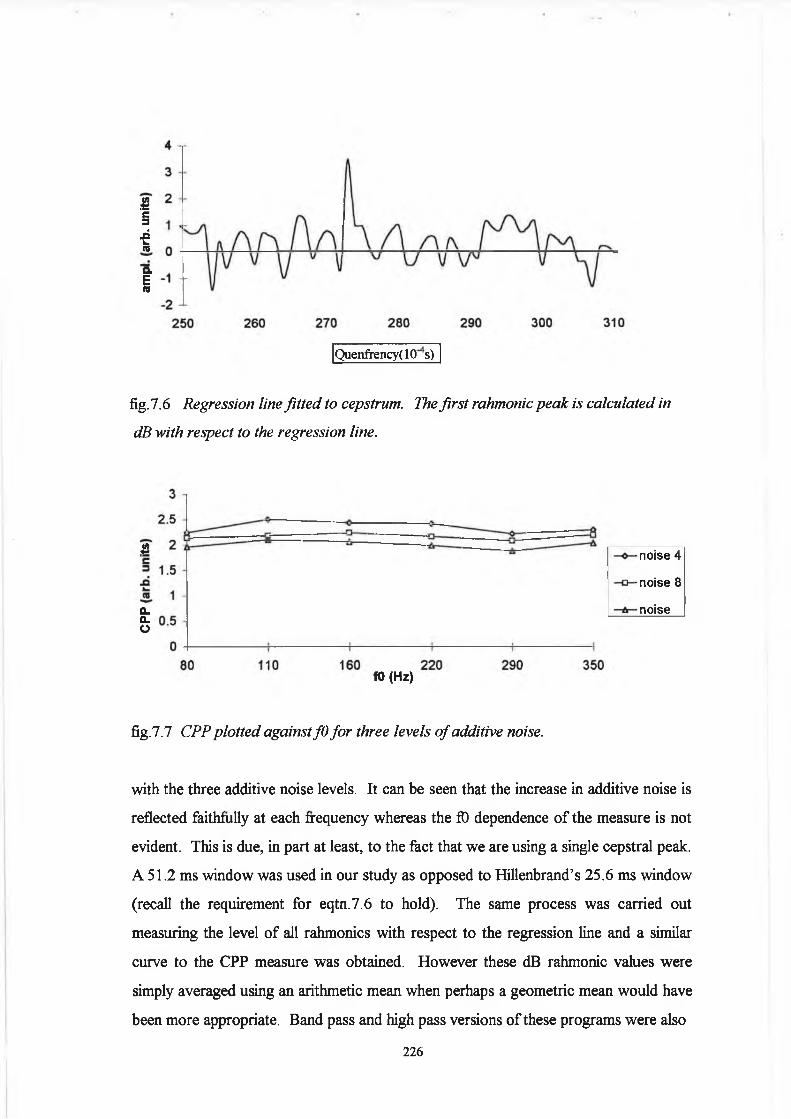
.3c3.dL.naEm

Quenfrency(10 s)

fig. 7.6 Regression line fitted to cepstrum. The first rahmonic peak is calculated in

dB with respect to the regression line.

£

a.a.o

-noise 4

-noise 8

-noise

fO (Hz)

fig. 7.7 CPP plotted against fO fo r three levels o f additive noise.

with the three additive noise levels. It can be seen that the increase in additive noise is

reflected faithfully at each frequency whereas the fO dependence o f the measure is not

evident. This is due, in part at least, to the fact that we are using a single cepstral peak.

A 51.2 ms window was used in our study as opposed to Hillenbrand’s 25.6 ms window

(recall the requirement for eqtn.7.6 to hold). The same process was carried out

measuring the level o f all rahmonics with respect to the regression line and a similar

curve to the CPP measure was obtained. However these dB rahmonic values were

simply averaged using an arithmetic mean when perhaps a geometric mean would have

been more appropriate. Band pass and high pass versions o f these programs were also

226

run on the data but for the CPP measure the filtered versions did not reflect the noise

increases. Hillenbrand did not employ a pitch tracking routine in implementing his

technique and found that not only did this have no adverse effects it actually increased

the breathiness prediction indicator. However, we found it essential to locate the

actual rahmonic peaks, especially in the case when using all rahmonics, otherwise the

method was found to give more erratic results (fig.7.8).

noise 4 -D -n o ise 8

- a- noise 16

110 160 220 290 350fO (Hz)

fig. 7 .8 CPPrah vs fO showing increased variability due to absence o f pitch tracking.

Hillenbrand interpreted his results to mean that since reduced CPP correlated very well

with breathiness, that aperiodicity is a strong indicator of breathiness. Although not

explicitly stated the implication is strongly taken to refer to periodicity o f the signal in

the time domain. However, we feel that the reduced rahmonic peak in breathiness is

not due to aperiodicity o f the time domain waveform. One o f the main indicators of

breathiness has often been reported to be an increased first harmonic amplitude12 along

with aspiration noise. The former acoustic parameter (increased fO amplitude) has

direct aerodynamic and physiological correlations in the form o f increased volume

velocity and more abducted vocal folds respectively. So, it is a well accepted

breathiness indicator. In the case o f breathy signals the reduced amplitude o f the

cepstral peak is also primarily due to the increase in the amplitude of the first harmonic.

To understand this, we see that the periodicity in the frequency domain is offset by this

increase in fO amplitude, leading to a less obvious ‘separation o f the log’. We note then

that periodicity in one domain does not necessarily indicate periodicity in another. On

227

the contrary, we observe that a sharp peak in one domain corresponds to a more

broadened (sinusoidal) event in the other domain (in fact, this is the reverse o f the

cepstrum). Therefore, perfect periodicity (sinusoid) can exist in the time domain and

yet no cepstral peak is found at the expected quefrency location. This in no way limits

the cepstrum for investigating breathy signals, on the contrary, Hillenbrand found an

excellent correlation but our inference is that this is due to the exploitation o f the

reduced ability to ‘separate the log’ and has little to do with aperiodicity in the time

domain. The response o f the H / N s , CPPrah and CPP indices to all perturbation

measures is shown in fig.7.9 (a), (b) and (c).

-noise -shimm er -cyclic jitter -random jitter

jitter std.dev.1-6% and 1-6 % shimmer and

additive noise std.dev. 1-32%

-shimmer

-noise

-cyclicjitter

-randomjitter

jitter std.dev.1-6% additive noise and

shimmer std.dev.1-32%

fig.7.9 (a) H/Ns and (b) CPPrah vs perturbation measures, where noise is more

linearly reflected fo r H/Ns with both methods being sensitive to random jitter.

228

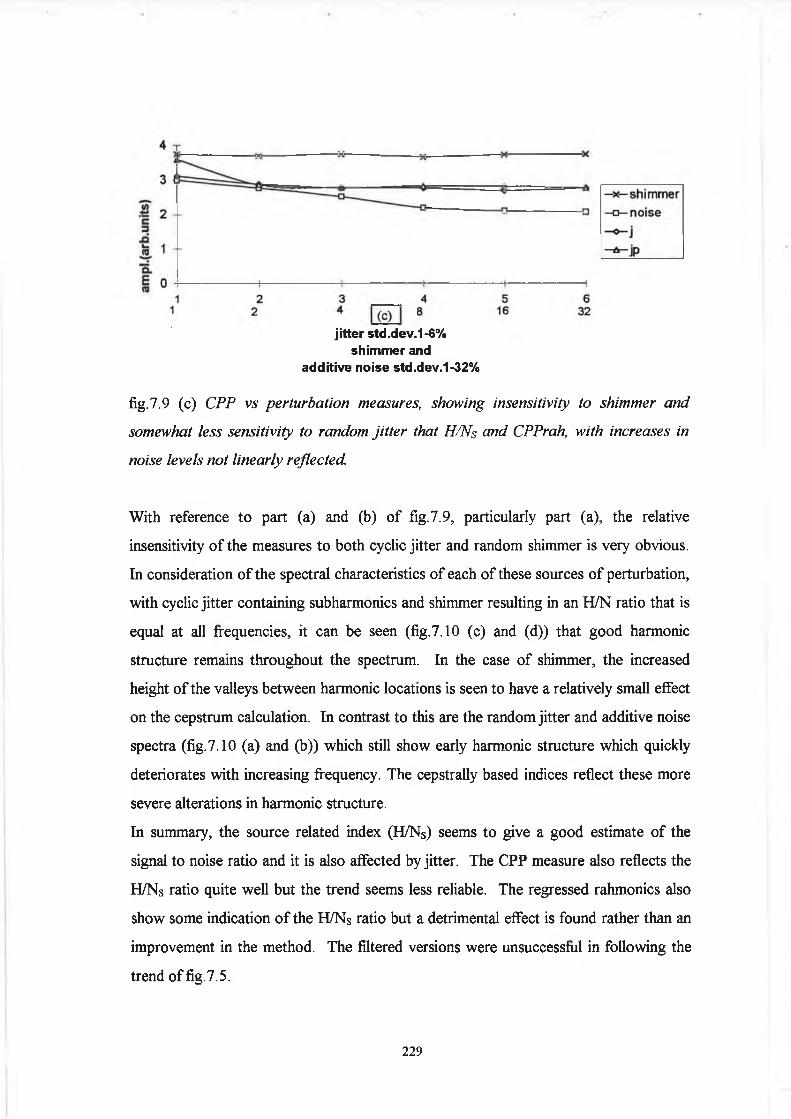
jitter std.dev.1-6% shimmer and

additive noise std.dev.1-32%

fig.7.9 (c) CPP vs perturbation measures, showing insensitivity to shimmer and

somewhat less sensitivity to random jitter that H/Ns and CPPrah, with increases in

noise levels not linearly reflected.

With reference to part (a) and (b) o f fig.7.9, particularly part (a), the relative

insensitivity o f the measures to both cyclic jitter and random shimmer is very obvious.

In consideration o f the spectral characteristics o f each o f these sources o f perturbation,

with cyclic jitter containing subharmonics and shimmer resulting in an H/N ratio that is

equal at all frequencies, it can be seen (fig.7.10 (c) and (d)) that good harmonic

structure remains throughout the spectrum. In the case o f shimmer, the increased

height o f the valleys between harmonic locations is seen to have a relatively small effect

on the cepstrum calculation. In contrast to this are the random jitter and additive noise

spectra (fig.7.10 (a) and (b)) which still show early harmonic structure which quickly

deteriorates with increasing frequency. The cepstrally based indices reflect these more

severe alterations in harmonic structure.

In summary, the source related index (H /N s) seems to give a good estimate o f the

signal to noise ratio and it is also affected by jitter. The CPP measure also reflects the

H /N s ratio quite well but the trend seems less reliable. The regressed rahmonics also

show some indication o f the H /N s ratio but a detrimental effect is found rather than an

improvement in the method. The filtered versions were unsuccessful in following the

trend offig.7.5.

229

(a)

frequency (Hz) (b)

0 1000 2000 3000 400020 T

-100 J-

frequency (Hz)(c)

0 10CX} 2000 3000 4000

frequency (Hz)(d)

fig.7 .10 Spectra fo r (a) 8 % std. dev. additive noise, (b) 4% stddev. random jitter, (c)

4% cyclic jitter cmd (c) stddev. 8 % random shimmer.

230

All methods were applied to the patient data in attempt to separate the patients from

the normals (fig.7.11 and fig.7.12). The CPP method shows reasonable ability in

separating the patient/normal data set with it’s filtered versions showing no

discriminatory ability. The regressed rahmonics show some degree of separability.

However, the source related harmonic to noise ratio (H/Ns) gives the best overall

discrimination, being highly significant at the 5 % level (one tailed, equal variance, two

sample mean, student’s t-test). Two encouraging hypotheses are made based on these

results : firstly, the method is potentially a good indicator o f vocal pathology (fig.7.11)

and secondly, the synthesis files are in some way representative o f the artifacts found in

actual vocal pathologies.

0 2 0.36 0.5 0.66 0.8 0.95 1.1 1.25 1.4H/Ns

fig.7 .11 Source related H/Ns index showing good separability o f the patient/normal

data set. (Highly significant at the 5% level using a one tailed, two sample, equal

variance, student’s t-test).

231

6

41 4 O C

| 3U UO 2

L L1.3

I

I pat. Inrm.

1.5 17 19 2 1 2.3

CPP (dB)(a)

2.5 2.7 2.9

3

L I

I pat. Inrm.

5.5

CPP

5

® 4Uc¡ 3ooO 2

1.1 1.2

fig.7.12 CPP measures (a) firs t rahmonic (CPP), (b) all rahmonics (CPPrah) and (c)

bandpassed, CPPb, with (a) and (b) showing significant (at the 5% level) separability

o f the patient/normal data set but not as high as H/Ns.

85 10 11.5 13 145

(all rahmonics) (dB)(b)

1.3 1.4 15

CPP band passed (dB) (c)

■ pat.■ nrm.

232

7.4 Conclusion:

1. A new cepstral measure, the source related harmonic to noise ratio (H/Ns) has been

defined and tested on tested on synthetically generated signals and also on a set o f

patient and normal productions o f the vowel aJ.

2. The height o f the cepstral rahmonics have been shown to be directly related to the

harmonic to noise ratio o f the ‘source related spectrum’, where the source related

spectrum can be obtained, for example, by comb littering the cepstrum and

subtracting the result from the original log spectrum.

3. The reduction in the ability to ‘separate the log’ when signals become more

dominantly sinusoidal (i.e. reduced richness o f harmonics) has been proposed as an

index for breathiness.

4. The H / N s has been shown to be a potentially useful indicator o f vocal pathology,

reflecting additive noise levels accurately and discriminating between a set o f 13

patients with varying vocal pathologies and a group o f 12 ‘normals’ with statistical

significance.

5. Absence of pitch tracking and band passing result in less reliable indices.

In conclusion, the cepstrum seems to offer three (although perhaps not completely

independent) indices for evaluating vocal pathology, namely, the H Z N ratio as

implemented by de Krom, the H / N s ratio as developed in this chapter and the

‘separation o f the log’ factor taken advantage o f by Hillenbrand. Future studies

might include other measures taken from the ‘source derived spectrum’.

The main points can be summarised as follows:

I

233

7.6 Bibliography

1. Bogert, BP. et al In M. Rosenblatt (Ed.) Proc. o f the Symp. On time series analysis.

NY: John Wiley and Sons 1963, pp.209-243

2. Schroeder, MR. Vocoders: Analysis and synthesis o f speech. Proc. IEEE 1966; 54:

720-734

3. Noll, AM. Cepstrum pitch determination. J. Acoust. Soc. Am. 1966; 293-309

4. Deller, J. Proakis J. and Hansen, J. Discrete time processing o f speech signals, NY:

Macmillan, 1989

5. Furui, S. Cepstral analysis technique for automatic speaker verification. IEEE

Trans, on Acoust., Speech and Signal Processing 1981; 29: 254-272

6. Oppenheim, A.V. and Schafer, R.W. Discrete-time signal processing. Englewood

Cliffs, N.J.: Prentice Hall, 1989

7. Koike, Y. and Kohda, J. The effect o f vocal fold surgery on the speech cepstrum.

In J. Gaufin and B. Hammarberg (Eds.) Vocal fold physiology: Acoustic, perceptual

and physiologic aspects o f voice mechanisms. San Diego: Singular Publ. 1991

8 . J. Hillenbrand, J. et al Acoustic correlates o f breathy vocal quality. J. Speech and

Hear. Res. 1994; 37: 769-777

9. de Krom, G. A cepstrum based technique for determining a harmonics-to-noise

ratio in speech signals. J. Speech Hear Res. 1993; 36: 254-266

10. Deller JR. et al Discrete time processing of speech signals, New York:Macmillan,

1993

11.Kasuya, H. et al Normalised noise energy as an acoustic measure to evaluate

pathologic voice. J. Acoust. Soc. Am. 80: 1329-1334

12. Klatt, DH. and Klatt, LC. Analysis, synthesis and perception o f voice quality

variations among female and male talkers. J. Acoust. Soc. Am. 1990; 87: 820-857

234

Conclusion

Presently used acoustic indices provide useful supplementary evidence for

documenting pathological voice types. The finding as laid out in the present thesis

support this fact, showing that indices do exist that separate pathologic voice types

from ‘normal’ voices. For example, bandlimiting the frequency range from 1-4 kHz

and calculating the harmonic to noise ratio appears to provide a reliable indicator of

dysphonia. Also, new indices have been introduced in this thesis that successfully

separate pathologic voice types from ‘normal’ voices. However, as presently

implemented, these indices offer only limited information regarding the exact physical

nature o f the voice disorder.

In order to achieve the ultimate goal of providing accurate clinical diagnoses o f voice

disorders, further basic research is required i.e. research that relates more specifically

to the relationship between anatomical events and the resultant acoustic sound pressure

waveform. This requires better knowledge of physiological function during phonation,

the extraction o f pertinent information from the acoustic speech waveform and a clear

understanding o f the relationship between the acoustic speech waveform and the

underlying vibratory pattern.

In spectral analysis o f pathological voice types, the gross spectral features o f jitter,

shimmer and additive noise, contaminate useful spectral information relating to the

vibratory pattern o f the vocal folds. This problem has been addressed in two ways.

Firstly, the spectral characteristics o f jitter, shimmer and additive noise have been

determined. Therefore, based on this information, pertinent spectral measures will

reveal what perturbation type is present. Secondly, a pitch synchronous harmonic

235

intensity analysis approach has successfully been developed to eliminate the effects o f

the perturbation measures and therefore provide more reliable information regarding

the vibratory pattern o f the vocal folds. Simple models have proven very useful for

providing quantitative information regarding speech-like material. However, in

conjunction with modelling, more research regarding the physiological and

neurological bases o f voice disorders is required, as well as improved correlations

between specific voice pathology types and acoustic findings. The final word is left to

Ingo Titze:

“There is a fallacy in trying to characterise the voice by a single number. There is a very complex

pattern in the voice signal, and this is the thing that we should be attempting to describe. After

viewing the voice in all it’s complexity and leaning more about it’s subtleties, then we may be in a

position to return and attempt to describe the voice through one or two measures. Prior to this, we

have to spend time just looking at the voice, say as one views a picture of the vocal folds or of vocal

fold movements. After we look at enough pictures, maybe then we will be in a better position to come

up with the few quantitative measures that are the most useful for describing the vocal folds during

voice production”1.

Bibliography:

1. Titze, IR. In PJ. Davis and NH. Fletcher (Eds.) Vocal Fold Physiology: Controlling

Complexity and Chaos, San Diego: Singular Pubi., 1996 pp.417

236

Appendix A

Source Code for Principal Matlab Program Files

A .l Time Domain Analysis

A. 1.1 ppitch3.m

%%%%%%%%%%%%File: PPitch3.m %% Name: Peter Murphy %% Date: Mon. 24_02J97%% Descr. A time domain pitch extraction method based on zero crossings, +ve & -ve % peaks% from a low passed filtered version of the acoustic speech signal.% The pitch ampl. is also returned via PPs% Call: [Noutp,Noutn,Noutl,Nout2,fointlpp,fointlnp,folpp,folnp,sPPs ] =% PPitch3(sp);%%%%%%%%%%%

function [Noutlp;Noutln,Noutll,Noutl2,fointlpp,fointlnp,folpp,folnp,fointpp,fointnp,fopp,fonp,sPPs] = PPitch3(sp);

hop = 100; fsam = 10000;

i

PERC = 0.4; fsam= 10000;

%%%%% Band pass filter the waveform (FIR (200-300)). (60Hz-hp)% Set the rough markers (-ve going zero crossings) for pitch extraction.%%%%

[sect] = sonasect(sp);

[fl)_est,nout] = fester2(sect,hop);

% l=fs/2 i.e. 5000 Hz ... 0.1=500 Hz.

b = firl(250,[2*60/fsam,2*1.5*f0_est/fsam]);I = filtfilt(b,l,sect);

length(l);

j=i;for i=l:length(l)-l % Obtain the number ofif l(i)>0&l(i+l)<0 % negative going zero crossings.

%NZC.zc_in(j) = i ;j=j+i;endend

NZC=j-l

P(1)=0;PP(1) = 0;PPs(l)=0;forj=2:NZC-l;[y,in] =sort(l(zc_in(j-l):zc_in(j)));[sy,sin] = sort(sect(zc_in(j-l):zc_in(j)));P(j)=zc_in(j-l)+in(l);PP(j)=zc_in(j-l)+in(length(l(zc_in(j-l):zc_in(j))));Ps(i)=zc_in(j-l)+sin(l);PPs(j) = zc_in(j-l)+sin(length(l(zc_in(j-l):zc_in(j))));PPrl(j) = PP(j)+(-0.5*(l(PP(j)+l)-l(PP(j)-l)))/(l(PP(j)+l)-2*l(PP(j))+l(PP(j)-l));pria)= p(j)+(-o.5ni(P(j)+i)-i(P(j)-i)))/(i(P(j)+i)-2*i(P(j))+i(pa)-D);PPsrl(j) = PPs(j)+(-0.5*(sect(PPs(j)+l)-sect(PPs(j)-l)))/(sect(PPs(j)+l)-2*sect(PPs(j))+sect(PPs(j)-

i));% Psrl(j) = Ps(j)+(-0.5*(sect(Ps(j)+l)-sect(Ps(j)-l)))/(sect(Ps(j)+l)-2*sect(Ps(J))+sect(Ps(j)-l));

end% Poly interpolation % PERC error detection

forj=6:NZC-4fintpp(j-5) =fsam/(PPsrl(j)-PPsrl(j-l));

% fmtnp(j-5) =fsam/(Psrl(j)-Psrl(j-l)); fhp(j-5) =fsam/(Ps(j)-Ps(j-1)); fpp(j-5) =fsamy(PPs(j)-PPs(j-l)); fintlpp(j-5)=fsani/(PPrl(j)-PPrl(j-l)); fintlnp(j-5)=fsam/(Prl(j)-Prl(j-l));

ii

flnp(j-5) =fsam/(P(j)-P(j-l)); flppO-5) =fsam/(PP(j)-PP(j-l)); end

sPPs=sect(PPs(2 :length(PPs)));

% Last check!!!% Make sure that the fOs fall within an acceptable level.%PERC

fointlpp=fmtlpp( fintlpp<mean(fintlpp)+mean(fintlpp)*PERC&fintlpp>mean(findpp)-PERC*mean(fintlpp));disp('no. of outliers');Noutp = length(fintlpp)-length(fointlpp)fointlnp=fintlnp( fmtlnp<mean(fmtlnp)+mean(fintlnp)*PERC&fintlnp>mean(fintlnp)-PERC*mean(fintlnp));disp('no. of outliers');Noutn = length(fmtlnp)-length(fointlnp)folpp=flpp( flpp<mean(flpp)+mean(flpp)*PERC&flpp>mean(flpp)-PERC*mean(flpp)); disp{'no. of outliers');Noutl = length(flpp)-length(folpp)folnp=flnp( flnp<mean(flnp)+mean(flnp)*PERC&flnp>mean(flnp)-PERC*mean(flnp)); disp('no. of outliers');Nout2 = length(flnp)-length(folnp)fointpp=fintpp( fintpp<mean(fintpp)+mean(fintpp)*PERC&fintpp>mean(fintpp)-PERC*mean(fintpp));disp('no. of outliers');Noutp = length(fintpp)-length(fointpp)%fointnp=fintnp( fintnp<mean(fintnp)+mean(fmtnp)*PERC&fintnp>mean(fintnp)-PERC*mean(fintnp));%disp('no. of outliers');%Noutn = length(fintnp)-length(fointnp)fopp=fpp( fpp<mean(fi^5)+mean(fpp) *PERC&ipp>mean(fpp)-PERC *mean(fpp)); disp('no. of outliers');Noutl = length(fpp)-length(fopp)fonp=fhp( fiip<mean(fhp)+mean(fhp)*PERC&fnp>mean(fhp)-PERC*mean(fhp)); disp('no. of outliers');Nout2 = length(fhp)-length(fonp)plot(fointpp);hold onplot(fointlpp,'r'); hold off pause

HR)=sect(PPs(6:NZC-4)); % index of original waveform +ve peaks Hf01=l(PP(6 :NZC-4)); % index of low pass +ve peaks

plot(HfO); hold on plot(HfDl,'r'); hold offdispCPerturbation measures from unfiltered waveform');[app,rapp,appp,stdndfO,PF 1 ,PF2,DPF,stdnd2fO,stddfD] = supperbl(fointpp); dispCPerturbation measures from filtered waveform'); [app,rapp,appp,stdndfl),PFl,PF2,DPF,stdnd2fO,stddfO] = supperbl(fointlpp);

iii

disp('Ampl.Pertuibation measures from unfiltered waveform');[aap,raap,apap,stdndHfO,HPFl,HPF2,DHPF,stdnd2Hf,stddHfl),dBdHfO] = amperel(abs(Hfl))); %disp('Ampl.Perturbation measures from filtered waveform');%[aap,raap,apap,stdndHfO,HPFl,HPF2,DHPF,stdnd2Hf,stddHfO,dBdHfO] = amperel(abs(Hf01)); % 5. Mean first order perturbation

% dHf01=diff(Hf01);% HPF1 = mean(abs(dHf01)./two_pt(HfDl))*100;% fprintfCHPFl(HfDl) = %.4f\n',HPFl);

% PF1 = mean(abs(diff(fointpp))./two_pt(fointpp))*100; % fprintfCPFlpp = %.4f\n',PFl);

% PF1 = mean(abs(diff(fointlpp))Vtwo_pt(fointlpp))*100; % fprintfCPFlppl = %.4f\n',PFl);

%[l,fowav] - wavmat(sect,fO_est);[Noutl,Nout2,fintlpc,fipc] = pzclpit(sect,fl)_est);

A. 1.2 pperb.m

%%%%%%%%%%%%%%%%%%%%%%%%%%%%%%%%%%%%%%%%%%%%%%%%%%%%%%%%%%0/0%%0/0 % % % % % % % % % % % % % 0/0

%% Program: pperb.m Matlab program to calculate the pitch variation % or perturbation factor.%% Name: Peter Murphy%%% Date: Mon. 24-02-'97%% Aim: To calculate the pitch perturbation in the speech signal%% Call: [app,rapp,appp,stdndfl),PFl,PF2,DPF,stdnd2fO,stddfD] = pperb(fD);%%%%%%%%%%%%%%%%%%%%%0/o%%%%%%%%%%%%%%%%%%%%%%%%%%%%%%%%%%%%%%%%%%%%%%%%%%%%%%%

% To calculate an indices for jitter (period/fl) perturbation).

function [app,rapp,appp,stdndfö,PFl,PF2,DPF,stdnd2fD,stddfö] = pperb(fO);

% pitch measurements

%dispCflO measurements'); mfö=mean(fO); sfl)=std(fO); mdfl)=median(fl));

% fprintf('aver. fundamental freq. = %6.3f\ri, mfO); % fprintf('std fO = %6.3f\n', sfD);

iv

% fprintf('median fO = %6.3f\n', mdfO);

dfO=diff(ffl); d2fl) =diff(dfO);

% pertuibation analysis % 1. average pitch pertuibation (app)

ap(F=mean(abs(dfl)));

% 2. relative average pitch pertuibation

rapp = mean(abs((three_pt(fD))-ffl(2:length(f0)-l)))/mean(fD)*100;

% 3. average percentage pitch pertuibation

appp = mean(abs(df0)./ffl(2:length(f0)))*100;

% 4. standard deviation of the pitch pertuibation divided by fO

stdndfO = std(dfO./two_pt(fO));

% 5. Mean first order perturbation

PF1 = mean(abs(df0)./two_pt(f0))*100;

% 6. Mean 2nd order pertuibation

PF2 = mean(abs(d2f0)./three_pt(f0))*100;

% 7 Directional pertuibation factor

k=0;

for i = I:length(df0)-1

if dfO(i)X)&dfO(i+1 )<0|df0(i)<0&dfD(i+1 )>0

t= k + l;

end

end

DPF = k/length(dfl))*100;

% 8 standard deviation of second order pitch pertuibation divided by fO

stdnd2f0 = std(d2fD./three_pt(fD))->

% 9 standard deviation of dfO

lA

‘.(.siusinamsBaui CÖH.)dsip

s;uouiojtisE3ui apruijdure ip jid %

•(C0H)qJ3d«re = [®HPaP1C8HPPís‘JHZpnpis‘j <iH a ^ 1ádH‘ládH ‘(0HPnpíSídEdB‘dBBj‘dBB] uopounj

(uoxjBqnmad apmiiduiB qj) jouiuiiijs ioj saotput ub sjBjnojBO ox %

%%%%%%%%%%%%%%0/o0/o%%0/o%%%%%%%%0/o%0/o%0/o%%%%%%%%%

•((SH)V9di«B

% = [(HHPeP‘(ÔHPPïs‘JH3PnpîstiIdHatddHÎJdH‘Q}HP«Pîs‘dBdB‘dBBi‘dBB] ìrbo %

j b u S i s i [ 33o d s d i p u i u o t i B q i r u j a d a p n j i i d u i K q o j i d o q i a i e p i o p » o x : u t r v %

L6rZO-fZ uopv :31Bq ®/o

vCqdmj jalad laurea %

jopBj uoiiBqjnyad %

apnjUduin qojid aip ajBpiojBO 01 ureiSojd qnpt^ uiqiadinE :uiBjSojy %

%%%%%%%%%%%%%%%%%%%%%%%%%%%%%%%%%%%%%%%%%%%%%%%%%%%%%%%%%%%%%%%%%%%%%%%%%%%%

u i qjsduiB £T V

X [ Q j p u i ( f l S Q j u i C t f p p j s Q i z p u p í s ¿ d a D d s i p

■ ( . Q j p u t c f l s Q j u i Q j p p j s ( t f z p u p j s J d a , ) d s i p

• ( [ Z d d l i d ( g p u p i s d d d B d d B J d d c ] ) d s i p

•(, ZJd l id Qfpupis d d d B ddBJ ddB ,)dsip

X , s a i n s B 9i u u o c j e q i t t u a d ^ i p %

%%%%%

u u o j u u n q o o u i s j j n s o j Á B j d s i a %

%

%%%%% ■(aiP)Pls = CflPPls

mHfl)=mean(HfO);

sHfO=std(HfO);

mdHfO=median(HfO);

% fprintf('ampl. fundamental freq. = %6.3f\n', mHfO);

%fprintf('std. HfD = %6.3f\n', sHfD);

% fprintffmedian HfD = %6.3f\n', mdHfD);

dHfO=diff(HiO);

d2HfD =diff(dHfO);

% amplitude perturbation analysis

% 1. average amplitude perturbation (aap)

aap=mean(abs(dHfO));

% 2. relative average pitch amplitude perturbation

raap = mean(abs(three_pt(HfD)-HfD(2:length(HfD)-l)))/mean(HlD)*100;

% 3. average percentage pitch amplitude perturbation

apap = mean(abs(dHTO)./HfO(2:length(HfO)))* 100;

% 4. standard deviation of the pitch amplitude perturbation divided by ffl

stdndHfO = std(dHf0./two_pt(Hf0));

% 5. Mean first order perturbation

HPF1 = mean(abs(dHf0)./two_pt(Hf0))* 100;

% 6. Mean 2nd order perturbation

HPF2 = mean(abs(d2Hf0)./three_pt(Hf0))* 100;

% 7 Directional amplitude perturbation factor

k=0;

vii

for i = l:length(dHfO)-l

i f dHfO( i)X)&dHfO(i+1 )<0|dHfl)(i)<0&dHf0(i+1 )>0

k=k+l;

aid end

DHPF = k/length(dHfO)* 100;

% 8 standard deviation of second order pitch amplitude perturbation divided by HfD

stdnd2Hf = std(d2HfD./three_pt(HfD));

% 9 standard deviation of dHfD

stddHfO = std(dHfO);

% 10 Average power differences-dB

dBdHfD = mean(diff(20*logl0(Hf0)));

% Display results in row form

dispCPertuibation measures');

disp(' aap raap apap stdndHfl) HPF1 HPf2 ' );

disp( [aap raap apap stdndHfD HPF1 HPF2 ]);

disp(' DHPF stdnd2Hf stddHfD dBdHfD ');

disp([ DHPF stdnd2Hf stddHfl) dBdHfi) ]);

disp(' mHfD sHfO mdHfl) ');

disp([mHfD sHfD mdHfD ]);

A.2 Harmonic Intensity Analysis

A.2.1 Noise Reducing Filter

% Program: Kitnos5.m %% Date : Thurs. 21-04-'97 %% Call: [NR,dBNR,geoNR]=kitnos5(sp);%% Name: Peter Murphy%% Aim: A modified version of Kitajima's method of using % a mov-av filter to estimate the noise levels.% The no. to aver depends on fO.% Combines kit3&kit4 to give 3 ratios.%%%%%%%%%%%%%

function [fsect,hsect,mavstd,nsect,NR,dBNR,geoNR]=kitnos5(sp);

pad = 2048; fsam = 10000; olap= 1024; f_cut= 3800; df =fsam/pad; len = 2048;

% [sectl] = sonasect(sp); [sect2] = sonastar(sp,3*len);

fsect = psd(sect2,pad,fsam,len,olap)'; fsect2= psd(sect2,pacysam,512)'; dBfsect = 10*logl0(fsect);[f0_est,nout] = fester2(sect2,olap); fOestm_avlen=round(f0_estydf)-2; if rem(floor(m_avlen),2)=0 m_avlen=m_avlen+1; end

% m_avlen=81;[m stdsect, m avfsect] = mov_av(fsect,m_avlen);

%%%%%%%%%%%

% Use the filtered spectrum to eliminate the % noise energy.%%%%%%%%%%%

mavstd=m_avfsect+m_stdsect;

for i= l :length(fsect)

if fsect(i)>(mavstd(i));

hsect(i) = fsect(i)-(mavstd(i));

else

hsect(i)=0;

endend

%%%%%%%%%%%% Now, use the filtered spectrum to estimate the % noise energy.%%%%%%%%%%%

for i= 1 :length(fsect)

if fsect(i)>(mavstd(i));

nsect(i) = (mavstd(i));

else

nsect(i)=0;

endend

elfplot(dBftect(l :500)); pause hold on

dBfsect2=10*logl0(fsect2); plot(dBfsect2(l :500),'r'); hold on

plot(10*logl0(hsect(l iSOO)),^); titleCNoise Reduced Periodogram'); hold onplot(10*logl0(nsect(l:500)),'b,);

N R = ( (mean(hsect.A2)).A0.5/mean(nsect.A2).A0.5);

dBNR=10*logl0(NR);hold offpauseelf[hsect,mavstd,geoNR]=kitdB(dBfsect,m_avlen); fprintfCNR=%6.3f\t',NR); $rintf('dBNR=%6.3f\n',dBNR);

A.2.2 Harmonic Intensity (Hiraoka)

%%%0/00/0%%%%%%%%%%%%%%%%0/0%%%%0/0%%% Program: harmony4.m%% Date: 03-03-'97%% Call: [Hr,Sr,dBH,dBS] = harmony4(sp_data);%% Note: make len =2048 and% padded to 4096. Test db ratio.%%%%%%%%%%%%%%%%%%0/o%%%%%%%%%%

function [spec_amp,Hr,Sr,dBH,dBS] = harmony4(sp_data);

% Let the operator choose the region for analysis as usual. % variables:

olap=100; f_cut=3800; fsam= 10000; pad=4096; len=2048; df=fsam/pad; bw=3*pad/len;

% Plot the speech sample % Choose the region for analysis % (Less than .4096 s)% Plot the spectrum for this region % (padded out to 4096)

subplot(3,l,l);sonagram(sp_data,fsam);[x y] = ginput(l);data= sp_data((x( 1) *fsam): (x( l)*fsam+len-1));subplot(3,l,2);sonagram(data,fsam);[spec_amp,spam] = specam2(data,pad); subplot(3,l,3); specplot(spec_amp,pad); disp('Press return to close figure window');

pausee lf

% length(spec_amp)% subplot(3,l,l);% dBplot(

% Plot the spectrum from 70 to 400 Hz % Determine fl) from the usual cepstral analysis.

speclow = spec_amp((70/df): (400/df));subplot(3,l,2);plot(speclow);

[f0,nout] = fester2(data,olap); fO

% Find the harmonic frequencies and sum the energies at these frequency % locations (exclude fl)).% Find the total signal energy.% Hence determine the relative harmonic intensity (Hr).

% Total Harmonic Amplitude (THAl-incl. fO, THA-excl. fO) % Total Signal Amplitude (TSA)

spec_har=zeros(size(spec_amp(l:f_cut/df+bw)));

THA1=0;THAldB=0;for i= 1: (f_cut/f0) % Determine no. harmonicsfor n=-bw: 1 :bw % Determine bwTH A I = THAl+spec_amp(i*fl)/df+n).A2; spec_har<i*f0/df+n)=spec_amp(i*fl)/df+n).A2;THAldB = THAldB+10*logl0(spec_amp(i*fD/df+n).A2);

endend

disp('lengths');Iength(spec_amp)length(spec_har)length(spec_amp( 1: f_cut/df+bw))

spec_nos=spec_amp( 1 :f_cut/df+bw).A2-spec_har;spec_nos=spec_nos(spec_nos~=0);spec_har=spec_har(spec_har~0);mHA=mean(spec_har);mHAdB=mean( 10 *log 10(spechar));mNA=mean(spec_nos);mNAdB=mean(10*logl0(spec_nos));

TSA=sum(spec_amp(l :f_cut/df). A2); mS A=mean(spec_amp( 1 :f_cut/df). A2); TSAdB=sum(10*logl0(spec_amp(l:f_cut/df).A2)); mSAdB=mean(10*logl0(spec_amp(l:f_cut/df).A2));THA= THAl-sum(spec_amp(i0/df-bw:i0/df+bw).A2);

xii

subplot(2,l,2);[dbspec] = dBplot(spec_amp,pad);

% dispCRelative Harmonic Intensity ='); dispCHr=');Hr = THA/TSA*100 ;% disp('Sr=');Sr = THA1/TSA*100;

HN = 10*logl0(THAl/(TSA-THAl));H2N = 10*logl0(THA/(TSA-THA));SN = 10*logl0(TSA/(TSA-THAl));

for i= 1: (fsam/2/fl))-1z(i) = max(specamp);endpauseelf

% subplot(2,l,l);plot(300:600,I0*Iogl0(spec_amp(300:600)),'g*'); hold onplot(300:600,10*logl0(spec_amp(300:600))); hold off

%%%%%%% S/N ratios %%%%%%

HNgeo = mHAdB-mNAdB;

% 1-3.8kHzhar_14=zeros(size(spec_amp( 1 :f_cut/df)));

THA14=0;THAdB14=0;for i=round(1000/fl)):round(f_cut/ffl) % Determine no. harmonics for n=-bw:l:bw % Determine bwTHA14=THA14+spec_amp(i*fO/df+n).A2;THAdB14=THAdB14+10*logl0(spec_amp(i*fD/df+n).A2);har_14((i-10()0/fO+l)*fD/df+n)=spec_amp(i*fiO/df+n).A2;endendTHA14THAdB14

length(spec_amp(1000/df:f_cut/df));length(har_14);

%nos_14=spec_amp(1000/df:f_cut/df).A2-har_14;%nos_14=nos_14(nos_14~=0);

xiii

har_14=har_14(har_14~=0);mHA14=mean(har_14);mH AdB 14=mean( 10 * log 10(har_ 14»;%mN A 14=mean(nos_ 14);%mNAdB14=mean(10*logl0(nos_14));

TSA14=sum(spec_amp(roimd(1000/f0)*fD/df-bw:round(f_cut/f0)*fD/df+bw).A2)TSAdB14=sum(10*logl0(spec_amp(round(1000/df):roimd(f_cut/df))A2));

HN_14 = 10*logl0(abs(THA14)/abs(TSA14-THA14));SN_14 = 10*logl0(abs(TSA14)/abs(TSA14-THA14));

% HN14geo = mHAdB14-mNAdB14;

Sr_14=THA14/TSA14*100;

%%%%% Display ratios%%%%

%OUT=[Hr;Sr;HN;H2N;SN;HNgeo;Sr_14;HN_14;SN_14;HN14geo];%disp(t,Hr '; 'Sr '; B N '; 'H2N ';'SN '; BNgeo '; 'Sr_14 '; BN_14 ';'SN 14';BN14geo']);%sprintf(' %f\n',OUT)fprintfCHr=%.3f\t',Hr); fprintf('Sr=%.3f\t',Sr); fjjrintf(BN=% . 3f\t\HN);^rintf(B2N=%.3f\t',H2N);fprintf('SN=%.3f\t',SN);%fprintf(,HNgeo=%.3f\n',HNgeo);%fprintf(’Sr_14=%.3f\t',Sr_14);%Q)rintf(BN_14=%. 3f\t',HN_l 4);%fprintf('SN_14=%.3f\t',SN_14);%l^rintf('HN 14geo=%. 3 f\n',HN 14geo);

A.2.3 Periodogram Averaged Analysis (PAHA)

%%%%%%%%%%%%%0/o%%%%%%%%%%%%%%

%

% Program: harmper2.m

% Date: 03-03-'97

%

% Call: [hsdB,Hr,Sr] = harmper2(sp_data);

%

% Note: make len =2048 and

xiv

% padded to 4096. Test db ratio.

%%%%%%%%%%%%%%%%%%%%%%%%%%%%

function [pdgram,hsdB,Hr,Sr,dBH,dBS] = harmper2(sp_data);

% Let the operator choose the region for analysis as usual.

% variables:

olap=100;

f_cut=3800;

fsam = 10000;

pad = 4096;

len = 2048;

df=fsam/pad;

bw=6*pad/len;

% Plot the speech sample

% Choose the region for analysis

% (0.2048 s)

% Plot the spectrum for this region

% (padded out to 4096)

[spdata]=sonastar(sp_data>5000);

[fD,nout] = fester2(spdata,olap);

10

[data] = sonasect(sp data); % Mouse click about 1 second in length

[Pxx,f] = psd(data,pad,fsam,Ien,len/2);

elf

plot(f,Pxx);

% Plot the spectrum from 70 to 400 Hz

% Determine fO from the usual cepstral analysis.

speclow = Pxx((70/df):(400/df));

subplot(3,l,2);

plot(speclow);

xv

% Find the harmonic frequencies and sum the energies at these frequency

% locations (exclude fO).

% Find the total signal energy.

% Hence determine the relative harmonic intensity (Hr).

for i=l:f_cut/fD[peaks(i),locs(i)] = pkpicker( Pxx( i*round(ffl/df)-bw:i*round(f0/df)+bw),le-300,l);

locs(i)=locs(i)+round(i*(fl)/df)-bw)-l ;

end

% Total Harmonic Amplitude (THAl-incl. fD, THA-excl. fO)

% Total Signal Amplitude (TSA)

spec_har=zeros(size(Pxx(l :f_cut/df+bw)));

THA1=0;

THAldB=0;

for i= 1: (f_cut/fD) % Determine no. harmonics

for n=-bw: 1 :bw % Determine bw

TH A I = TH A 1+Pxx(locs(i)+n);

THAldB = THAldB+10*logl0(Pxx(locs(i)+n));

spec_har(locs(i)+n)=Pxx(locs(i)+n);

end

end

for i=l:(f_cut/fO)

har min(i) = min(Pxx(locs(i)-bw:locs(i)+bw)); % spectrum derived Source spectrum

harm ax(i) = max(Pxx(locs(i)-bw:locs(i)+bw));

hs(i) = har_max(i)/har_min(i);

length(hs);

hsdB=10*logl0(hs);

HNS= 10*logl0(mean(hs));

HNSO1=10*logl0(mean(hs(l: 1000/f0)));

HNSl4=10*logl0(mean(hs(1000/fD:f_cut/f0-l)));

RHNS14=10*logl0(mean(hs(l:1000/f0)/mean(hs(1000/fl3:f_cut/f0-l)))); % subtract HNS01-HNS14

(same)

xvi

HNShl_5=10*logl0(mean(hs(l:5)));

HNSh6_l l=10*logl0(mean(hs(6:11)));

HNShl l=10*logl0(m ean(hs(l:l 1)));

RHNSh6_5=10*logl0(mean(hs( 1:5))/mean(hs(6:11)));

disp('lengths');

length(Pxx(l :f_cut/df+bw));

length(spechar);

% spec_nos=Pxx(l:f_cut/df+bw)-spec_har;

% spec_nos=spec_nos(spec_nos~=0);

% spec_har=spec_har(spec_har~=0);

subplot(2,1,1)

title('source spectrum derived from output waveform spectrum');

plot(hsdB);

subplot(2,l,2)

('isolation of harmonics from output waveform spectrum')

plot(10*logl0(spec_har));

% mHA=mean(spec_har);

% mHAdB=mean(10*logl0(spec_har));

% mNA=mean(spec_nos);

% mNAdB=mean(10*logl0(spec_nos));

TSA=sum(Pxx(l :f_cut/df+bw));

TSAdB=sum(10*logl0(Pxx(l :f_cut/df+bw)));

THA= THAl-sum(Pxx(locs(l)-bw:locs(l)+bw));

THAdB=THAldB-sum(10*logl0(Pxx(locs(l)-bw:locs(l)+bw)));

subplot(2,l,2);

plot(f,Pxx);

titleCPeriodogram averaged spectrum');

xlabel('freq. (Hz)');

ylabel('amplitude (arb units)');

dispCRelative Harmonic Intensity =');

disp('Hr=');

Hr = THA/TSA*100;

xvii

dispCSi=');Sr = THA1/TSA*100;

HN = 10*logl0(THAl/abs(TSA-THAl));

H2N = 10*Iogl0(THA/abs(TSA-THA));

SN = 10*logl0(TSA/abs(TSA-THAl));

for i=l:(fsam /2/fö)-l

z(i) = max(Pxx);

end

% subplot(2,l,l);

pdgram= 10* log 10(Pxx);

plot(f(300:6()0),10*logl0(Pxx(300:600)),,*,);% hold on

% plot(f(300:600),10*logl0(Pxx(300:600)),'g');

title('modificd periodogram estimate');

xlabcl('freq.(Hz)');

ylabel('ampl.(dB)');

%%%%%%% S/N ratios

%%%%%%

% HNgeo = mHAdB-mNAdB;

% 1-3.8kHz

har_ 14=zeros(size(Pxx( 1000/df: f_cut/df+bw)));

THA14=0;

THAdB14=0;

for i=roimd(1000/iö) : (f_cut/fl)) % Detennine no. harmonics

for n=-bw: 1 :bw % Determine bw

THA14=THA14+Pxx(Iocs(i)+n);

THAdB 14=THAdB 14+10*logl0(Pxx(locs(i)+n));

xviii

har_14((locs(i)- 1000/fö+ l)+n)=Pxx(locs(i)+n);

end

end

dispOlengths');

length(Pxx(1000/df:f_cut/df+bw));

length(har_14);

% nos_14=Pxx(1000/df:f_cut/df)-har_14;

% nos_14=nos_14(nos_14~=0);

% har_14=har_14(har_14~=0);

% mHA14=mean(har_14);

% mHAdB14=mean(10*logl0(har_14));

% mNA14=mean(nos_14);

% mNAdB14=mean(10*logl0(nos_14));

TS A l 4=sum(Pxx(round( 1000/fl))*f[)/df-bw:roimd(f_cut/i0)*fl)/df+bw));

TSAdB14=sum(10*logl0(Pxx(1000/df:f_cut/df)));

H N 14 = 10*logl0(THA14/(TSA14-THA14));

S N 14 = 1 O*logl 0(TS A 14/(TS A l 4-THA14));

% HN14geo = mHAdB14-mNAdB14;

Sr_14=THA14/TSA14*100;

%%%%

% Display ratios

%%%%

fprintfCHr=%.3f\t',Hr);

iprintf('Sr=%.3f\t',Sr);

iprintf(’HN=%.3f\t’,HN);

iprintf('H2N=%.3At',H2N);

fprintf('SN=%.3f\n',SN);

%fprintf('HNgeo=%. 3f\n',HNgeo);

fjprintf('Sr_14=%.3f\t',Sr_14);

fprintf('HN_14=%.3f\t',HN_14);

fprintf('SN_14=%.3f\t',SN_14);

fprintf(’HNS=%. 3f\t',HNS);

xix

fprintf(HNS14=%.3f\t',HNS14);

fprintf('HNS01=%.3f\n',HNS01);

fprintfCRHNS 14=%.3f\t',RHNS 14);

fprintf(’HNShl_5=%.3f\t',HNShl_5);

fprintfCHNSh6_l l=%.3f\t',HNSh6_l 1);

fprintf('HNShl 1=%. 3f\t’,HNShl 1);

fprintf(rRHNSh6_5=%.3fji',RHNSh6_5);

%fprintf('HN14geo=%.3f\n',HN14geo);

A.2.4 Pitch Synchronous (Four Periods)

%%%%%%%%%%%%%%%%%

% Date: Tues. 04-03-'97

% Program: Harm4_2.m

% Call: [LMTN,H,LOCS,dBH,NS] = harm4_2(sp);

%

% Descr. Finds the noise to harmonic ratio for a signal by examining four

% pitch periods. The ratio is in dBs. ft) is first calculated from

% the cepstrum and then a better estimate is attained using zcs on

% a lp filtered waveform.

%

% Name: Peter Murphy

%

%%%%%%%%%%%%%%%%

function [LMTN,H,LOCS,dBH,NS] = harm4_2(sp);

fsam= 10000;

hop=100;

PERC=0.4;

x x

nh=l6;

%%%%%%%% Choose region for intended analysis %%%%%%%%%%

[sect]=sonastar(sp,7500);

%%%%%%%% Obtain initial fO estimate %%%%%%%%%%

[fD_est,nout] = fester2(sect,hop);

fDest

% l=fs/2 i.e. 5000 Hz ... 0.1=500 Hz.

b = firl(250,[2*60/fsam,2*1.5*fl)_est/fsamj);

1 = filtfilt(b,l,sect);

length®;

j=i;for i= 1 :length(l)-l % Obtain the number of

if l(i)>0& l(i+ l)<0 % negative going zero crossings.

% NZC.

zc_in(j) = i ;

j=3+l;end

end

NZC=j-l

P(1)=0;

forj=2:NZC -l;

ty,in] =sort(l(zc_in(j-l):zc_in(j)));

P(j)=zc_in(j-l)+in(l);

end

% Poly interpolation

% PERC error detection

for j=5:NZC-l

xxi

flnp(j-4)=fsam/(P(j)-P(j-l));

end

% Last check!!!

% Make sure that the fOs fall within an acceptable level.

% PERC

folnp=flnp( flnp<mean(flnp)+mean(flnp)*PERC&flnp>mean(flnp)-PERC*mean(flnp));

disp('no. of outliers');

Nout2 = length(flnp)-length(folnp)

P=P(4:NZC-1); % Indices for the pitch periods

NPM=NZC-4; % in sect.

%%%%%%%%% Calculate the Power Spectrum %%%%%%%%%%

for i=l:NPM -4

plen = P(i+4)-P(i);

harms = abs(ffl((sect(P(i):P(i+4)-l)).*hamming(plen)) ).A2/plen;

H (l:plen/2+l,i) = harms(l:plen/2+l)';

df(i)=fsam/plen;

end

%%%%%%%%%%%%%%%% Calculate

%%%%%%%%%%%%%%%%%%%%%

%%%%%%%%%%%%%%%%%%%%%%0/o%%%%%0/o%%%%0/o%0/o%

for j=l:N PM -4

fori= l:nh

[peaks(i),locs(i)] = pkpicker( H( i*roimd(fl)_est/df(j))-2:i*round(ffl_est/df(j))+2j),le-300,l);

LOCS(ij)=locs(i)+round(i*(fO_est/df(j))-2)-l;

end

end

the N /H ratio for the first

16 harmonics.

xxii

forj=l:NPM -4

for i=I:nh

[pmin(i),lmin(i)I = min( H (LO CS(io)-l:LO CS(ij)+2));

LM IN(ij)=lm in(i)+LO C S(ij)-2;

end

end

N=sum(sum(H(LMIN)));

S=sum(sum(H));

NS=10*logl0(N/S);

for j=l:size(M,2)

Nsseg(j) =10*logl0( sum(H(LMIN(: j)))/sum(H(: j ) ) );

Nin=length(Nsseg);

Nsseg=Nsseg(

abs(Nsseg)<median(abs(Nsscg))+median(abs(Nsseg))*PERC&abs(Nsseg)>median(abs(abs(Nsseg)))-

PERC*median(abs(Nsseg)));

disp('no. of outliers');

Nout=Nin-length(Nsseg)

Nsseg;

NSseg=mean(Nsseg);

NSsegstd=std(Nsseg);

H=H+le-100; % Avoid logl0(0)

dBH=10*logl0(H);

%waterfall(dBH(3:66,:)')

%pause

plot(dBH(3:66, l),'r*')

hold on

plot(dBH(3:66,l))

pause

xxiii

sum(dBH);

mean(dBH);

dBS=mean(mean(dBH));

dBN=mean(mean(dBH(LMEN)));dBNS=dBN-dBS;

forj=l:size(H,2)

dBNsseg(j) =( mean(dBH(LMIN(: j ) ) )-mean(dBH(: j ) ) ) ;

end

dBNSseg=mean(dBNsseg);

dBNS sstd=std(dBNsseg) ;

gSN=10*logl0( sum(sum(dBH))/sum(sum(dBH(LMIN))) );

forj=l:size(H,2)

gSnseg(j) =10*logl0( sum(dBH(: j))/siun(dBH(LMIN(: j) ) ) );

gSnseg;

gSNseg=mean(gSnseg);

gSNsstd=std(gSnseg);

%OUT=[NS;NSseg;NSsegstd;dBNS;dBNSseg;dBNSsstd;gSN;gSNseg;gSNsstd];

%disp([,NS 'jTSTSseg VNSsegstdVdBNS YdBNSseg ';'dBNSsstd';'gSN VgSNseg VgSNsstd

']);%sprintf(' %(\n',OUT)

fprintf('NS=%. 3f\t',NS);

fprintf(rNSseg=%.3f\t',NSseg);

fprintf('NSsegstd=%.3f\t',NSsegstd);

fprintf(’dBNS=%.3f\t\dBNS);

íprinlf('dBNSseg=%. 3f\t',dBNSseg);

fprintf('dBNSsstd=%.3ñn’,dBNSsstd);

fjprintf('gSN=%.3f\t',gSN);

fprintf('gSNscg=%. 3f\t',gSNseg);

fprintf('gSNsstd=%.3f\t',gSNsstd);

XXIV

A.2.5 Normalised Noise Energy

%%%%%%%%%%%%%%%%%%%°/o%%%%%%%%%%%%%%

% Program: Noise6.m

%

% D ate: w e d 2 2 -01 -’9 7

% Call: [NS] = noise6(sp);

%

% Name: Peter Murphy

% Aim: To estimate the ratio of noise to total signal energy

% for a speech signal. This is a revamp of noise2.m in

% to evaluate the NNE at each segment, not just the

% last.

%%%%%%%%%%%%%%%%%%%%%%%%%%%%%%%

function [dB_Mmean,NS,Ml,M2,M3,M4] = noise6(sp);

pad = 2048;

fsam = 10000;

olap = 200;

fc u t = 3800;

df=fsam/pad;

kilo = 1000;

hop = 100;

[sect2] = sonasect(sp);

[T0_est,nout] = festerl(sect2,hop); % Make an initial estimate of ID

K)_est=l/T0_est; % using ckcorr.m

TI=7*T0_est*fsam; % From this est. we take 7 pitch

n0_segs=(length(sect2)-TT)/olap; % periods-the analy.length.

BW=round(2*pad/TI);

%f0_est=109.89;

XXV

for i=l:nO_segs

seg= sect2(l+i*olap:TI+i*olap);

fseg= (abs(fft(seg.*hamming(n),pad)).A2)’;

M (:,i) = (fseg(l:f_cut/df+BW));

dB_M(:,i) - 10*logl0(fseg(l:f_cut/df+BW+5)); % dB_M contains the spectra in

% columns.

end

elf

% waterfall(dB M');

% pause

% elf

dB_Mmean=mean(dB_M( 100:200,:)');

plot(mean(dB_M(100:200,:)'));

% hold on

% plot(mean(dB_M(200:300,:)'),'r*');

title('dB spectrum of mean frequencies taken over the section');

% [peaks,Iocs] = pkpicker(dBfseg,Q.001,f_cut/fl)_est);

fori= l:14

z(i)= max( dB_M (l:130,2));

end

% elf

% plot(dBfseg,'r');

% hold on

% stem(locs,z);

% pause

% hold off

forj=l:n0_segs

for n=l:f_cut/fO_est

[peaks(n),locs(n)] = pkpicker( dB_M( (round( 1+n*(fO_est/di)-BW ):roimd(l+n*(ffl_est/df)+BW)

)J),-100,1);

LOCS(nj)=locs(n);

xxvi

end

end

forj=l:nO_segs

for n=l:f_cut/fl)_est

LOCS(nj) = round( l+n*(fl)_est/df)-BW -l+LOCS(nj)); % shift=index into array -1.

end

end

% Location of harmonic peaks

% at j-th spectrum.

%%%%%%%%%

% Plot one of the resulting spectra to

% show that the peaks have been deter-

% mined correctly.

%

%%%%%%%%%

% elf

% pIot(dB_M(( 1:130),2),’r*');

% hold on

% plot( dB_M ((l:130),2));

% hold on

% stem(LOCS( 1:14,2),z( 1:14»;

% pause

% hold off

%%%%%%%%

% Establish the harmonic peak regions. i.e. Take the BW eith

% -er side of n harmonic peaks.

%%%%%%%

xxvii

for j=l :size(LOCS,2)

for i= l :size(LOCS, 1)

P((i-l)*(2*BW+l)+l:i*(2*BW+l)J) = (LOCS(ij)-BW:LOCS(ij)+BW)';

end

end

%%%%%%%%

% Establish the between harmonic regions, i.e. Take from

% k+BW to k+l-BW .

% This region is made up of the pad/2+1 points less the

% P points (Also less the point up to the 1st harmonic)

%

%%%%%%%

M1=M;

M2=M;

M2(P)=zeros(size(P));

%%%%%%%%%%%

%% Now estimate the noise energy in the

% harmonic regions.

%%%%%%%%%%%%

for j=2 : size(LOCS,2)

for i=2 :size(LOCS, 1)-1

M l(LO CS(lj)-BW :LO CS(lj)+BW j)=m ean(M (LO CS(lj)+BW +l:LO CS(2j)-BW -

l)).*ones(size(LOCS(lj)-BW :LOCS(l,j)+BW ))';

xxviii

if(M (L (X :S (i-lj)+B W +l:LO C S (ij)-B W -l))==[]|(M (LO C S (ij)+B W +l:LO C S (i+ lj)-B W -l))==[]

M l(LOCS(ij)-BW :LOCS(ij)+BW j)=m ean(m ean((M(LOCS(i-lj)+BW +l:LOCS(i-

1 j)+BW +l)))+m ean((M (LOCS(ij)+BW +l:LOCS(ij)+BW +l)))).*ones(size(LOCS(ij)-

BW:LOCS(ij)+BW))';

elseM l(LOCS(ij)-BW :LOCS(ij)+BW j)=m ean(m ean((M(LOCS(i-lj)+BW +l:LOCS(ij)-BW -

l)))+mean((M(LOCS(ij)+BW +l:LCX3S(i+l ji-BW -l^^onesCsizeiLOCSiiji-BW XOCSOji+BW ))';

end

%%%%% Same for 1st column.

%%%%

for i=2:size(LOCS,l)-l

M l(LO CS(l,l)-BW :LO CS(l,l)+BW ,l)=m ean(M (LO CS(l,l)+BW +l:LO CS(2,l)-BW -

1)). *ones(size(LOCS( 1,1 )-B W :LOCS( 1,1)+B W))';

if( M (LOCS(i-l, 1)+BW+1 :LOCS(i,l )-BW -1) )==[]|(M (LOCS(i,l)+BW +l:LOCS(i+l,l)-BW -

1))==D

Ml(LOCS(i,l)-BW :LOCS(i,l)+BW ,l)=m ean(m ean((M(LOCS(i-l,2)+BW +l:LOCS(i-

l,2)+BW+l)))+mean((M(LOCS(i,2)+BW+l:LOCS(i,2)+BW+l)))).*ones(size(LOCS(i,2)-

BW:LOCS(i,2)+B W))';

else

Ml(LOCS(i, 1)-BW :LOCS(i, 1)+BW, l)=mean(mean((M(LOCS(i-l, 1)+BW+1 :LOCS(i, 1)-BW-

l)))+mean((M(LOCS(i,l)+BW+l:LOCS(i+l,l)-BW-l)))).*ones(size(LOCS(i,l)- BW:LOCS(i,l)+BW))’;

end

end

xxix

%%%%%%%% If NaNs still exist remove that spectrum from

% both the signal & noise estimates.

%%%%%%%

M3=M;M4=M 1;for j= I:size(M l,2)

x= M l(:j);

i=U;

i=find(isnan(x));

if i~=0;M 1 (: j)=zeros(size(M 1,1), 1);

M (: j)=zeros(size(M, 1), 1);

end

end

forj=l:size(Ml,2) if Ml(:j)=0

M3(:j)=n;M4(:j)=[];

end

end

%%%%%%%%%%%%%

%1.% Sum the noise energy.

% Sum tlie signal energy.

% Calculate NNE.

%%%%%%%%%%%%%%

S = sum(sum(M3));

W = sum(sum(M4));

xxx

NS=10*logl0(W/S);

%%%%%%%% 2. Limit I-4kHz

%%%%%%%

M l_4 = M3(kilo/df:fcut/df,:);

M l 1 4 = M4(kilo/df:f_cut/df,:);

S14 = sum(sum(Ml_4));

W14 = sum(sum(Ml 1_4));

NS14=10*logl0(W14/S14);

%%%%%%%% Calculate 1.&2. above with dB ratios

%%%%%%%

dBM = l0*log!0(M 3);

dBM l= 10*logl0(M4);

N SdB=mean(mean(dBM 1 -dBM));

dBM 1 4 = 10*logl0(M l_4);

dB M ll_4= 10*logl0(M l 1_4);

NS 14dB=mean(mean(dBM 1 l_4-dBMl_4));

%%%%%%

% Calculate segmental means

%%%%%%

Nsseg= 10*logl0(sum(M4)./sum(M3));

NSseg=mean(Nsseg);

NSsegstd=std(Nsseg);

XXXI

fsam = 10000;

olap = 100;

f_cut = 3800;

len = 7250;

PERC=0.4;

%%%%%%%% Make an initial estimate of fD

% This analysis is to be performed on 3 successive cycles

% for 325ms.

%

%%%%%%

[i0_est,nout] = fester2(sp,olap);

fOest

df=fsam/(3 *fsam/fl)_est);

%%%%%%

%

% Choose region for analysis (325 ms).

%

%%%%%%

[sect] = sonastar(sp,len);

[m,pp,f,P,NPM] = zpitch3(sect,fl)_est);

% [sect,f,pp,NPMj = zpitch2(sect,f0_est);

% M = zeros(max(diff(P))*3/2,NZC/3 );

for j=2:3 :NPM/3-3

seg3pit = sect(pp(j):pp0'+3)-l);

fseg3pit = abs(fft(seg3pit)).A2';

% plot(fseg3pit(l :length(seg3pit)/2),'r,);pause

% x = l:length(seg3pit)/2; hold on

% stem(x,fseg3pit(l:length(seg3pit)/2));

% pause

% hold off

xxxiii

M ( 1: length(fseg3 pit)/2,(j+1 )/3) = fseg3pit(l:length(seg3pit)/2)/length(seg3pit);

dB_M(l:length(fseg3pit)/2,(j+l)/3) = 10*logl0( fseg3pit(l:length(seg3pit)/2)/length(seg3pit));

% dB_M contains the spectra in

% columns.

waterfall(M(l :f_cut/df,

pause

plot(10*logl0(mean(M( 1 : f _ c u t /d f , i * 1);

hold on

plot( 10*Iogl0( mean( M (l:f_cut/df,:)')));

hold off

S = [ M (l+3:3:f_cut/df,:) ];

N1 = [ M (l+l:3:f_cut/df-2,:) ];

N2 = [ M (l+2:3:f_cut/df,:) ];

R = 10*logl0( sum(sum(S))/( sum(sum(Nl))+sum(sum(N2))));

S_dB - [ dB_M(l+3:3:f_cut/df,:) ];

Nl_dB = [ dB_M(l+l:3:f_cut/df-2,:) ];

N2_dB = [ dB_M(l+2:3 :f_cut/df,:) ];

rseg=10*logl0( mean(S)./(mean(Nl)+mean(N2)))

Nin=length(rseg);

rseg=rseg( abs(rseg)<mean(abs(rseg))+mean(abs(rseg))*PERC&abs(rseg)>mean(abs(abs(rseg)))-

PERC*mean(abs(rseg)));

disp('no. of outliers’);

Nout=Nin-length(rseg)

Rseg=mean(rseg);

xxxiv

Rsegstd=std(rseg);

RdB = 10*logl0( mean(mcan(S_dB))-( mean(mean(Nl_dB))+mean(mean(N2_dB)) ) );

rdbseg=10*logl0( mean(S dB)-(mean(Nl_dB)+mean(N2_dB)) );

RdBseg=mean(rdbseg);

RdBsstd = std(rdbseg);

Rgco= 10*logl0( sum(sum(S_dB))/( sum(sum(N 1 _dB))+sum(suni(N2 dB)) ) );

rgcoscg= 10*logl0( sum(S_dB)./(sum(Nl_dB)+sum(N2_dB)) );

Rgeoseg= mean(rgeoseg);

Rgeosstd=std(rgeoseg);

%OUT=[R;Rseg;Rsegstd;RdB;RdBseg;RdBsstd;Rgeo;Rgeoseg;Rgeosstd];

%disp(['R 'illseg ';'Rsegstd ';'RdB ';'RdBseg ';'RdBsstd ';'Rgeo ';Tlgeoseg ’;'Rgcosstd']);

sprintf(' %f\n',OUT)

fprintfCR=%.3f\t',R);

fprintfCRseg=%. 3f\t',Rseg);

fprintf('Rsegstd=%. 3ñt',Rsegstd);fjprintf('RdB=%.3f\t',RdB);

fprintf('RdBseg=%.3f\t',RdBseg);

fpri ntf('RdBsstd=%. 3 f\n', RdBsstd) ;

fprintf('Rgeo=%. 3f\t',Rgeo);

fprintf('Rgeoseg=%.3f\t',Rgcoseg);

fprintf('Rgeosstd=%. 3f\n',Rgeosstd);

S_14 = [ S(1000/ffl_est:size(S,l),:) ];

N114 = [ Nl(1000/f0_est:size(Nl,l),:) ];N 2 1 4 = [ N2(1000/iD_est:size(N2,l),:) ];

R_14 = 10*logl0( sum(sum(S_14))/( sum(sum(Nl_14))+sum(sum(N2_14)) ) );

XXXV

S_dB14 = [ S_dB(1000/f0_est:size(S,l),:) ];

Nl_dB14 = [ Nl_dB(1000/fD_est:size(Nl,l),:) ];

N2_dB14 = [ N2_dB( 1000/fl)_est:size(N2,1),:) ];

rsegl4=10*logl0( mean(S_14)./(mean(Nl_14)+mean(N2_14)));

Nin=length(rsegl4);

rsegl4=rseg!4(

abs(rsegl4)<median(abs(rsegl4))+median(abs(rsegl4))*PERC&abs(rsegl4)>median(abs(abs(rsegl4))

)-PERC*median(abs(rsegl4)));

%disp('no. of outliers');

%Nout=Nin-length(rsegl4)

Rsegl4=mean(rsegl4);

Rsegl4d=std(rsegl4);

RdB14 = 10*logl0( mean(mean(S_dB14))-( mean(mean(Nl_dB14))+mean(mean(N2_dB14))));

rdbsegl4=10*logl0( mean(S_dB14)-(mean(Nl_dB14)+mean(N2_dB14)));

RdBsegl4=mean(rdbsegl4);

RdBsl4d = std(rdbsegl4);

Rgeol4=10*logl0( sum(sum(S_dB14))/( sum(sum(Nl_dB14))+sum(sum(N2_dB14)) ) ) ;

rgeosl4= 10*logl0( sum(S_dB14)./(sum(Nl_dB14)+sum(N2_dB14)));

Rgeosl4= mean(rgeosl4);

Rgeos 14d=std(rgeos 14);

%OUT=[R_14;Rsegl4;Rsegl4d;RdB14;RdBsegl4;RdBsl4d;Rgeol4;Rgeosl4;Rgeosl4d];

%disp([rR_14 ’;'Rsegl4 ,;'Rsegl4d ';'RdB14 ';'RclBsegl4';’RdBsl4d ';'Rgeol4 ';'Rgeosl4

,;rRgeosl4d']); sprintf(' %f\n',OUT)

xxxvi

fprintf('R_14=%.3f\t,,R_14);

fprintf('Rsegl4=%.3f\t',Rsegl4);

fprintf('Rseg 14d=%. 3 f\t',Rseg 14d);

fprmtf('RdB 14=%.3f\t',RdB14);

fprintf('RdBsegl4=%.3f\t',RdBsegl4);

fjprintf(’RdBsl4d=%.3f\n',RdBsl4d);

fprintf('Rgeo 14=%.3f\t',Rgeo 14);

fprintf(,Rgeosl4=%.3f\t,,Rgeosl4);

fprintf(rRgeosl4d=%.3f\t\Rgeosl4d);

A.2.7 Partial Sum of the Fourier Series (Two Period)

%%%%%%%%%%%%%%%%%%%%

% Program: psha2.m

% Date: Mon. 24-06-'97

% Call: psha2(sp);

% Name: Peter Murphy

%% Aim: To estimate the harmonic to noise ratio

% using Fourier Series Expansion. H /N cycle by cycle.

% psha2 = pitch sync. harm, analysis (l=lths3)

%%%%%%%%%%%%%%%%%%%%

function [S,N,P] = psha2(sp);

fsam = 10000;

olap= 100;

fc u t = 3800;

len = 7250;

xxxvii

FERC=0.4;

%%%%%%

% Make an initial estimate of ffl

% This analysis is to be performed on 2 successive cycles

% for 725ms.

%%%%%%

[fO_est,nout] = fester2(sp,olap);

fO_est

df=fsam/ (2*fsam/f0_est);

%%%%%%

% Choose region for analysis (725 ms).

%

%%%%%%

[sect] = sonastar(sp,len);

[in,ppXP,NPM] = zpitch3 (sect,iD_est);

% [sect,f,pp,NPM] = zpitch2(sect,f0_est);

% M = zeros(max(dilf(P))*3/2,NZC/3 );

forj=2:l:NPM -3

seg2pit = sect(pp0):pp0+2)-l);

fseg2pit = abs(fit(seg2pit)).A2';

% plot(fseg3pit(l :length(seg3pit)/2),,r,);pause

% x = 1 :length(seg3pit)/2; hold on

% stem(x,fseg3pit(l:length(seg3pit)/2));

% pause

% hold off

M(l:length(fseg2pit)/2 j-1 ) = fseg2pit(l:length(seg2pit)/2)/length(seg2pit);

dB_M(l:length(fseg2pit)/2j-l) = 10*logl0( fseg2pit(l:length(seg2pit)/2)/length(seg2pit));

xxxviii

end

% dB M contains the spectra in

% columns.

% waterfall(M(l:f_cut/df,:)');

% pause

% elf

% plot(10*logl0(mean(M(l:f_cut/df,:)')),'r*');

% hold on

stem( 10*logl0( mcan( M (l:f_cut/df,:)')));

% hold off

pause

S = [ M (l+2:2:f_cut/df,:) );

N = [ M (l+l:2:f_cut/df-2

size(S)

sizc(N)

if (size(S)==size(N))

hns= S( 1 :size(S, 1 )-1, :)./N( 1 :size(N, 1 )-1,

else

hns= S( 1 :size(S, l)-2 ,:)./N ( 1 :size(N, l)-l,:);

end

HNS = 10*logl0(mean(mean(hns)));

% waterfall(10*logl0(hns)’);

•M iause

% plot(10*logl0(hns(l:size(hns,l),l)));

%pause

% plot(10*logl0(hns(l:size(hns,l),2)));

9^>ause

% plot(10*logl0(hns(l:size(hns,l),3)));

%pause

% plot( 10*logl 0(hns( 1 : size(hns, 1),4)>);

%pause

plot(10*logl0(mean(hns(l :size(hns, I),:)1)));

hns_av = mean((hns(l:size(hns,l),0)');

xxxix

HNS01=10*logl0(mean(hns_av(l: 1000/f0_est)));

HNS 14= 10*logl0(mean(hns_av(1000/f0_est:f_cut/f0_est-2)));

RHNS14=10*logl0(mean(hns_av(l: 1000/f0_est)/mean(hns_av(1000/f0_est:f_cut/f0_est-2)))); %

subtract HNS01-HNS14 (same)

HNShl_5=10*logl0(mean(hns_av(l :5)));

HNSh6_l l=10*logl0(mean(hns_av(6:11)));

HNShl l=10*logl0(mean(hns_av(l: 11)));

RHNSh6_5=10*logl0(mean(hns_av(l :5))/mean(hns_av(6:11)));

R = 10*logl0( sum(sum(S))/sum(sum(N)));

S_dB = [ dB_M(l+2:2:f_cut/df,:) ];

N_dB = [ dB_M(l+l:2:f_cut/df-2,:) ];

rseg=10*logl0( mean(S)./mean(N))

Nin=length(rseg);

rseg=rseg( abs(rseg)<mean(abs(rseg))+mean(abs(rseg))*PERC&abs(rseg)>mean(abs(abs(rseg)))-

PERC*mean(abs(rseg)));

disp('no. of outliers');

Nout=Nin-length(rseg)

Rseg=mean(rseg);

Rsegstd=std(rseg);

RdB = 10*logl0( mean(mean(S_dB))-( mean(mean(N_dB))));

rdbseg=10*logl0( mean(S_dB)-(mean(N_dB)));

RdBseg=mean(rdbseg);

RdBsstd = std(rdbseg);

Rgeo= 10*logl0( sum(sum(S_dB))/( sum(sum(N_dB))) );

xl

rgeoseg= 10*logl0( sum(S_dB)./(sum(N_dB)) );

Rgeoseg= mean(rgeoseg);

Rgeosstd=std(rgeoseg);

%OUT=[R;Rseg;Rsegstd;RdB;RdBseg;RdBsstd;Rgeo;Rgeoseg;Rgeosstd];

%disp([,R 'i'Rseg ';'Rsegstd ';'RdB 'jTldBseg ';'RdBsstd 'i'Rgeo 'j'Rgeoseg 'jTlgeosstd']);

sprintfC %f\n',OUT)

fprintfCR=%. 3 f\t',R) ;

fprintf('Rseg=%. 3f\t',Rseg);

fprintf('Rsegstd=%. 3 f\t',Rsegstd) ;

fprintf('RdB=%. 3 f\t',RdB);

fjprintfCRdBseg=%.3f\n',RdBseg);

fprintf(rRdBsstd=%. 3f\t',RdBsstd);

fprintf('Rgeo=%. 3 f\t\Rgeo) ;

fjprintf('Rgeoseg=%.3f\t',Rgeoseg);

fprintfCRgeosstd=%.3f\n',Rgeosstd) ;

S_14 = [ S(1000/i0_est:size(S,l),:) ];

N_14 = [ N(1000/fl)_est:size(N,l),:) ];

R_14 = 10*logl0( sum(sum(S_14))/sum(sum(N_14)) );

S_dB14 = [ S_dB(1000/f0_est:size(S, 1),:) ];

N_dB14 = [N_dB(1000/f0_est:size(N,l),:) ];

rsegl4=10*logl0( mean(S_14)./mean(N_14) );

Nin=length(rsegl4);

rsegl4=rsegl4(

abs(rsegl4)<median(abs(rsegl4))+median(abs(rsegl4))*PERC&abs(rsegl4)>median(abs(abs(rsegl4))

)-PERC*median(abs(rsegl4)));

%disp('no. of outliers');

%Nout=Nin-length(rsegl4)

Rsegl4=mean(rsegl4);

Rsegl4d=std(rsegl4);

RdB14 = 10*logl0( mean(mean(S_dB14))-( mean(mean(N_dB 14)) ) );

rdbsegl4=10*logl0( mean(S_dB14)-(mean(N_dB14)) );

xli

RdBsegl4=mean(rdbsegl4);

RdBsl4d = std(rdbsegl4);

Rgeol4=10*logl0( sum(sum(S_dB14))/( sum(sum(N_dB14)) ));

rgeosl4= 10*logl0( sum(S_dB14)./(sum(N_dB14)));

Rgeosl4= mean(rgeosl4);

Rgeosl4d=std(rgeosl4);

A.2.8 Time Domain Averaging

%%%0/o%%0/o%0/o%0/o%0/o0/o%0/o%%0/o%%

% program: harmyuml.m

% date: Tues. 03-12-'96

% call: [M] = harmyuml(sp);

%

% Descr. finds the harmonic to noise ratio from the time domain signal.

%%%%%%%%%%%%%%%%%%%%%

function [M,P] = harmyuml(sp,np);

f_cut=3800;

fsam= 10000;

hop=200;

len= 10500;

olap=100;

%%%%%%%% Mouse pick the section again %%%%%%%%%%

[sect]=sonastar(sp,len);

%%%%%%%% Calculate an initial estimate of %%%%%%%%%%

%%%%%%%% fO using autocorrelation. %%%%%%%%%%

x l i i

[f0_est,nout] = fester2(sect,olap);

% [sectl,f,pp,NPM] = zpitch2(sect,f0_est);

[in,pp,f,P,NPM] = zpitch3(sect,fO_est);

%%%%%%%%%%%%%% Attain an average waveform %%%%%%%%%%%%

forj=5:NPM-5

M ( l:(pp0'+l)-pp(j))j-4) = sect(pp(j):ppG+l)-l)';

end

M =M (:,l:size(M ,2)-2);

snratio(M,np);

A.2.9 Pitch Synchronous Harmonic Analysis

%%%%%%%%%0/o0/o%%%0/o%%%%%0/o%%0/o%%%%%%%0/o0/o%%%%%

% Program: LTHS4 - long time harmonic spectrum

% Date: Thurs. 18-03-'97

% By: Peter Murphy

%

% call: [pp]=lths4(sp);

% Note: This program provides a convenient way to analyse

% how the ampl. of the 'harmonics' change with time.

% The changes to lthsl.m are 1. 1-3.8k range used.

% 2. global ratios are calc.

% every 50 periods & std taken.

% As per lths3 but padded to 512 pts.

%%%%%%%%0/0%%%%%%%%%%%%%%%%%%%%%0/0%%%%%%

function [pp]=lths4(sp);

fsam= 10000;

f_cut=3800;

len=7500;

hop=200;

np=50;

xliii

sft=10;

pad=512;

%%%%%

% Long time harmonic spectra -estimate the gross spectral features for a sample

% of speech. Note the addition is done wrt the harmonic freqs.

% Make an initial estimate of ID

%%%%%%

[fO_est.nout] = fester2(sp, 100);

%TO_est=220;

%%%%%%% Choose region for analysis.%%%%%%

[sect] = sonastar(sp,len);

[in.pp.f.P.NPM] = zpitch3(sect,fD_est);

% [sect,f,pp,NPM] = zpitch2(sect,f0_est);

% M = zeros(m in(difi(P))/2+l,NZC-l);

forj=l:NPM -5

segpit = sect(pp(j+2):pp(j+3)-l);

fsegpit = (abs(ffl(segpit,pad))/pad)‘; % Normalise wrt win. length

feegpit = (feegpit(l:pad/2+l)*f_cut/fsam*2)/max(fsegpit);

% stem(fsegpit); pause

% hold on

M(l:length(fsegpit)j) = fsegpit;

dB_M(l:length(fsegpit)j) = 20*logl0(fsegpit);

% dB_M contains the spectra in

% columns.

end

xliv

%clf

%fallspec(M’);

%pausc

%clf

avhspec = meaniM1);

%plot(mean(M'),'r’);

%hold on

%stem(mean(M'));

%holdoff

%pause

%clf

stem(mean(dB_M'));

plot(mean(dB_M,),'r');

pause

%%%%%%%%%% Amplitude Perturbation Ratios

%%%%%%%%%

APAP = mean(abs(diff(M(2, :))))/mean(M(2, :)); % Aver pere. pitch ampi, perturbation.

stdAPAP=std(abs(diff(M(2, :))))/mean(M(2, : )) ;

SHR = mean(abs(diff(dB_M(2,:)))); % Shimmer

stdSHR=std(abs(diff(dB_M(2, :))));

HAPAP = meaniabsidiffCMO^./meaniM1); % As per APAP but for all harmonics.

SHH = mean(abs(difF(dB_M'))); % " - SH " " " H

THAPAP = mean(HAPAP); % Aver over all freqs.

sTHAPAP= std(HAPAP);

TSHH = mean(SHH); % " " " ■ .

sTSHH = std(SHH);

%%%%%%%%%

% Signal to Noise Ratios

xlv

%%%%%%%%%

for i=I:(size(M,2)-np)/sft

M s=M (:,l+ (i-l)*sft:n i^(i-l)*sft);

As = mean(Ms');

AVs=As';

H - sum(sum(Ms.A2));

plot(AVs');

Ms_AV=[J;

for j=l:size(Ms,2)

Ms_AV = [Ms_AV AVs];

end

N = sum( sum( (Ms-Ms_AV).A2) );

Hn(i)=10*logl0(H/N);

end

HN=mean(Hn);

stdHN=std(Hn); %% HN

A = mean(M');

AV=A';

Hnseg=0;

for i= 1 :size(M^2)

Hmeg(i)=10*logl0(sum(M(:,i).A2)/sum((M(:,i)-AV).A2));

end %% HNseg

stdHNseg=std(Hnseg);

HNseg=mean(Hnseg);

for i= l :(size(dB_M,2)-np)/sft

dB_M s=dB_M (:,l+(i-l)*sft:np+(i-l)*sft);

dB As = mean(dBMs'); %% HNgeo

dBAVs=dBAs';

dBM_AVs=D;

for j=l:size(dB_Ms,2)

xlvi

dB M A Vs = [dBM_AVs dBAVs];

end

Hngeo(i) = 10 * log 10((mean(mean((abs(dB_Ms-dBM_ AVs))))));

dBHs = sum(sum(dB_Ms.A2));

dBNs = sum( sum( (dB_Ms-dBM_AVs).A2 ));

dBHn(i)= 10*logl0(dBHs/dBNs); %% dBHN

end

HNgeo=mean(Hngeo);

stdHNgeo=std(Hngeo);

dBHN=mean(dBHn);

stddBHN=std(dBHn);

%%%%%%%

% Distortion Factor

%%%%%%%

for i=l:size(M,2)

d(i)=sum(M(3 :size(M, l),i).A2)/M (2,i). A2;

end

DFl=mean(d); %%DF1

stdDFl=std(d);

for i=l:size(dB_M,2)

db(i)=sum(abs(dB_M(3 :size(dB_M, l),i)))/abs(dB_M(2,i));

end

DF2=mean(db); %% DF2

stdDF2=std(db);

%%%%%%%

% Lim it the spectral range & calculate the same ratios

xlvii

% from lk-f_cut Hz.

%%%%%%%

size(M)lD=fsam/min(diff(pp));

x=size(M,l);M14=M(1000/f0:x,:);

dB_M14=20*logl0(M14);

HAPAP14 = mean(abs(diff(M 14')))./mean(M 14’); % As per APAP but for all harmonics.

SHH14 = mean(abs(diff(dB_M14'))); % « " SH " " " H

THAPAP14 = mean(HAPAP); % Aver over all freqs.

sTHA14= std(HAPAP);

TSHH14 = mean(SHH); % " " "

STSHH14 = std(SHH);

%%%%%%%%%% Signal to Noise Ratios

%%%%%%%%%

for i= 1 :(size(M 14,2)-np)/sft

M sl4=M14(:,l+i*sñ:np+i*sft);

Asl4 = mean(Msl4');

AVsl4=Asl4';

H14 = sum(sum(Msl4.A2));

plot(AVsl4');

Ms_AV14=[];

for j= 1 :size(Ms 14,2)

Ms_AV14 = [Ms_AV14 AVsl4];

end

N14 = sum( sum( (M sl4-M s_AV14).A2 ));

Hnl4(i)=10*logl0(H14/N14);

end

HN14=mean(Hnl4);

xlviii

stdHN14=std(Hnl4); %% HN14

A14 = mean(M14‘);

AV14=A14';

Hnsegl4=0;

for i=l:size(M14,2)

Hnsegl4(i)=10*logl0(sum(M14(:,i).A2)/sum((M14(:,i)-AV14).A2));

end %% HNsegl4

HNsegl4=mean(Hnsegl4);

stdHNsl4=std(Hnsegl4);

for i=l:(size(dB_M14,2)-np)/sft

dB_Ms 14=dB_M14(:, l+i*sft:npH*sft);

dBAsl4 = mean(dB_Msl4'); %% HNgeo

dBAVsl4=dBAsl4';

dBMAVsl4=[];

for j= 1 :size(dB_Ms 14,2)

dBMAVsl4 = [dBMAVsl4 dBAVsl4];

end

Hngeol4(i) = 10*logl0((mean(mean(abs((dB_Msl4-dBMAVsl4))))));

dBHsl4 - sum(sum(dB_Msl4.A2));

dBNsl4 = sum( sum( (dB_Msl4-dBMAVsl4).A2) );

dBHnl4(i)=10*logl0(dBHsl4/dBNsl4); %% dBHN

end

HNgeo 14=mean(Hngeo 14);

stdHNgl4=std(Hngeo 14);

dBHN 14=mean(dBHn 14) ;

stdBHN 14=std(dBHn 14) ;

%%%%%%%%%

xlix

% Display the above:

%%%%%%%%%

fprintf('APAP=%.3f\t',APAP);

fprintf(' SHR=%. 3 f\t', SHR);

fprintf(THAPAP=%.3f\t',THAPAP);

fprintf('TSHH=%.3f\t',TSHH);

fjprintf('HN=%.3f\t',HN);

fprintfCHNseg=%.3f\n',HNseg);

fprintfCHNgeo=%. 3f\t',HNgeo);

fprintf('dBHN=%. 3 f\t',dBHN);

ijprintf(T)F 1=%. 3f\t',DF 1);

fprintf('DF2=%.3f\n',DF2);

fprintf('stdAPAP=%.3f\t',stdAPAP);

fprintf('stdSHR=%.3f\t',stdSHR);

fprintf('sTH AP AP=%. 3 f\t', sTHAP AP);

fprintf('sTSHH=%. 3f\t',sTSHH);

fjprintf('stdHN=%. 3f\t',stdHN);

fjprintf(,stdHNseg=%.3f\n',stdHNseg);

fprintf('stdHNgeo=%.3f\t,,stdHNgeo);

fprintf('stddBHN=%.3f\t',stddBHN);

fprmtf('stdDF 1=%. 3 f\t', stdDF 1);

fprintf('stdDF2=%.3f\n',stdDF2);

^mntf('THAPAP14=%.3f\t',THAPAP14);

fprintf('sTHA14=%.3f\t',sTHA14);

fprintf('TSHH14=%.3i\t',TSHH14);

fprintf('sTSHH 14=%. 3 f\t',sTSHH 14);

fprintf(’HN14=%.3f\t',HN14);

fprintf('stdHN 14=%. 3 f\n', stdHN 14);

fprintf('HNsegl4=%.3f\t',HNsegl4);

fjprintf('stdHNsl4=%.3f\t',stdHNsl4);

fprintf(TINgeol4=%.3f\t'rHNgeol4);

fprintf('stdHNgl4=%.3f\n',stdHNgl4);

fprintf('dBHN 14=%.3f\t',dBHN 14);

iprintf(fstdBHN14=%.3f\n',stdBHN14);

A.3 Long Term Average Spectrum Analysis

%%%%%%%%%%%%%%%%%%%%%%%%%%%%%%%%%%%%%%

%

% Program: LTAS3 - long term average spectra

%Date: Tues. 04-02-'97

% By: Peter Murphy

%

% call: [averspec] = ltas3(sp_data,lseg,hop,pad);

% Note: This is a copy of ltasl altered to obtain the

% difference between spectra.

%%%%%%%%%%%%%%%%%%%%%%%%%%%%%%%%%%%%%

function [longspec,a,b]=ltas3(sp_data,lseg,hop,pad);

fcu t = 3800;

% Long term average spectra-estimates the gross spectral features for a sample

% of speech.

[sect]=mousie(sp_data);

nsegs = (length(sect)-lseg)/hop;

elf

for i=l:(length(sect)-lseg)/hop

specamp = specampl(sect(l+(i-l)*hop:lseg+(i-l)*hop),pad);

M (l:pad/2+l,i) = specamp’.A2;

dB_M(l:pad/2+l,i) = 10*logl0(specamp'.A2);

end

waterfall(M');

litle('Linear spectra');

xlabel('freq');

ylabel('ampr);

li

pause

waterfaII(dB_M’);

pause

DM = diff(M');

D d B M = diff(dB_M');

waterfall(DM);

pause

waterfall(DdB_M);

pause

avspec = mean(M);plotspec(avspec,pad);

pause

plotdB(mean(dB_M'),pad);

title('dB spectrum of LT AS'); a=diff(avspec,2);

pauseplot(diff(diff(( 10*logl0(avspec)))>);

b=diff(diff((10*logl0(avspec))));

pause

plot(10*logl0(avspec));

pauseplot(mean(DM));

pause

lü

A.4 Cepstral Analysis

%%%%%%%%%

% Program: cpphnr.m To obtain the hnr for a speech sample using cepstral

% analysis. A comb liftered cepstrum is ffted to give a noise

% estimate.

% Name: Peter Murphy

%Date: Thurs. 27/02/’97

%

% call: [RP,CRAPP,CRAPPl,CN,dBCN] = cpphnr(sp,hop);

% lseg = 2048; hop = 256.

%%%%%%%%%

function [RP,CRAPP,CRAPPl,CN,dBCN] = cpphnr(sp,hop);

lscg=2048;

bw= 10;

cw= 10;

[sect] = sonastar(sp,5000);

for i = 1 :(length(sect)-lseg)/hop

[logh, c_sect] = cceps3(sect(l+i*hop:lseg+i*hop));

% Returns real cepstrum.

C(:,i) = c_sect';

0 (:,i) = logh';

end

% plot(((Hf))); % Graphing outputs.% title('cepstral peaks vs no. of hops'); % Cepstral peaks & Cepstrum.

% xlabel('no. hops');

liii

% ylabel('amplitude (linear)');

% pause;

% plot(20*logl0(c_sect)); % pause;

% dBc_sect = 20*logl0(c_sect);

% title(’cepstrum ampl. dB vs quefrency');

% xlabel('quefrency (ms)');

% ylabel('amplitude (dB)1);

% pause;

% elf

% 10k/25:10k/142 fieq range.

[Y,I]=max(C((25:142),:)); % Obtain the 1st rahmonic index

% for each cepstrum.

1=1+24;

1=29;

for i=l:size(C,2)

for j= 1 :size(C, l)/m ax(I)/2

[a,b]=max(C(j*I(i)-bw:j*I(i)+bw,i));

iiO)=t^ j* I(‘)-bw-l;

end

RP(: ,i) = ii'; % Rahmonic peaks RP

end % Each column contains the rah.

% peaks for that cepstrum.

for i= 1 :size(RP,2) % Mean Rahmonics amplitude (dB)

CRAPPl=C(RP(:,i),i);

end

CRAPP1 = mean(sum(CRAPPl);

C1=C;

Uv

forj=l:size(C,2)

for i=l:size(RP, 1) % Comb liftering

Cl(RP(i)-0.5*cw:RP(i)+0.5*cwj)=zeros(size(RP(i)-0.5*cw:RP(i)+0.5*cw))';

C l((l :40) j)=zeros(size(l :40))';

C l((2048-40:2048) j)=zeros(size(l :41))';

end

end

CN=sum(sum(Cl));

dBCN=10*logl0(CN);

fprintf('CRAPP = %6.3f\t', CRAPP);

fprintf('CRAPPl = %6.3i\t’, CRAPP1);

fprintf('CN = %6.3f\t',CN);

fjmntf(’dBCN = %6.3f\n',dBCN);

lv