Development of an Improved Group Contribution Method for ... · Development of an Improved Group Contribution Method for the Prediction ... 2.2.3.2 Lee-Kesler method ... using the

Development of an Improved Group

Contribution Method for the Prediction

of Vapour Pressures of Organic

Compounds

By

Bruce Moller [B.Sc.(Eng.)]

University of KwaZulu-Natal Durban

In fulfilment of the degree Master of Science (Chemical Engineering)

December 2007

i

ABSTRACT

Vapour pressure is an important property in the chemical and engineering industries. There are

therefore many models available for the modelling of vapour pressure and some of the popular

approaches are reviewed in this work. Most of the more accurate methods require critical property

data and most if not all require vapour pressure data in order to regress the model parameters. It is

for this reason that the objective of this work was to develop a model whose parameters can be

predicted from the molecular structure (via group contribution) or are simple to acquire via

measurement or estimation (which in this case is the normal boiling point).

The model developed is an extension of the original method that was developed by Nannoolal et al.

The method is based on the extensive Dortmund Data Bank (DDB), which contains over 180 000

vapour pressure points (for both solid and liquid vapour pressure as of 2007). The group

parameters were calculated using a training set of 113 888 data points for 2332 compounds.

Structural groups were defined to be as general as possible and fragmentation of the molecular

structures was performed by an automatic procedure to eliminate any arbitrary assumptions. As

with the method of Nannoolal the model only requires knowledge about the molecular structure and

the normal boiling point in order to generate a vapour pressure curve. In the absence of

experimental data it is possible to predict the normal boiling point, for example, by a method

developed by Nannoolal et al.

The relative mean deviation (RMD) in vapour pressure was found to be 5.0 % (2332 compounds

and 113 888 data points) which compares very well with the method of Nannoolal et al. (6.6 % for

2207 compounds and 111 757 data points). To ensure the model was not simply fitted to the

training set a test set of liquid vapour pressure, heat of vaporization and solid vapour pressure data

was used to evaluate its performance. The percentage error for the test set was 7.1 % for 2979

data points (157 compounds). This error is artificially high as the test data contained a fair amount

of less reliable data. For the heat of vaporization at 298.15 K (which is related to vapour pressure

via the Clausius-Clapeyron equation) the RMD was 3.5 % for 718 compounds and in the case of

solid vapour pressures the RMD error was 21.1 % for 4080 data points (152 compounds). Thus the

method was shown to be applicable to data that was not contained in the training set.

ii

PREFACE

The work presented in this dissertation was undertaken at the University of KwaZulu-Natal Durban

from January 2007 till December 2007. The work was supervised by Professor D. Ramjugernath

and Professor Dr. J. Rarey.

This dissertation is presented as the full requirement for the degree of Master of Science in

Engineering (Chemical). All work presented is this dissertation is original unless otherwise stated

and has neither in whole of part been submitted previously to any tertiary institute as part of a

degree.

_______________________

Bruce Moller (203502126)

As the candidates supervisor I have approved this dissertation for submission

_______________________

Prof. D. Ramjugernath

iii

ACKNOWLEDGEMENTS

I wish to acknowledge the following people and organizations for their contribution to this work:

• My supervisors, Prof. D. Ramjugernath and Prof. Dr. J. Rarey for tireless support, ideas and

motivation during this work. Working with them has been a privilege and a great learning

experience.

• Dr. Y. Nannoolal for helping me to get this work started.

• NRF International Science Liaison, NRF-Thuthuka Programme and BMBF (WTZ-Project)

for financial support.

• DDBST GmbH for providing data and software support for this project.

• My parents Erik and Jeanette, my sister Teresa, my grandmother and late grandparents for

all their years of wisdom and guidance. They have my eternal gratitude.

• Most importantly I would like to give praise to my Lord and Saviour Jesus Christ. “ … Praise

be to the name of God for ever and ever; wisdom and power are his. He changes times and

seasons; he sets up kings and deposes them. He gives wisdom to the wise and knowledge

to the discerning.” Daniel 2:20-21.

iv

TABLE OF CONTENTS

Abstract .................................................................................................................................................i

Preface ................................................................................................................................................. ii

Acknowledgements ............................................................................................................................. iii

Table of Contents ................................................................................................................................ iv

List of Figures.................................................................................................................................... viii

List of Tables ..................................................................................................................................... xiii

Nomenclature ................................................................................................................................... xvii

1 Introduction .................................................................................................................................. 1

2 Theory and Literature Review...................................................................................................... 3

2.1 Introduction ........................................................................................................................... 3

2.2 Vapour pressure models....................................................................................................... 4

2.2.1 Classical thermodynamics............................................................................................. 4

2.2.1.1 The Antoine equation............................................................................................ 8

2.2.1.2 The Cox equation and Cox charts ...................................................................... 10

2.2.1.3 The Riedel equation............................................................................................ 12

2.2.1.4 The Myrdal & Yalkowsky equation...................................................................... 14

2.2.1.5 The Tu group contribution method...................................................................... 16

v

2.2.1.6 The modified Watson equation ........................................................................... 19

2.2.2 Kinetic theory of vaporization ...................................................................................... 20

2.2.3 Equations of state........................................................................................................ 22

2.2.3.1 Alpha functions ................................................................................................... 22

2.2.3.2 Lee-Kesler method.............................................................................................. 25

2.2.4 Empirical models ......................................................................................................... 27

2.2.4.1 The Wagner equation ......................................................................................... 28

2.2.4.2 Quantitative structure property relationship........................................................ 29

2.2.4.3 Interpolation polynomials .................................................................................... 30

2.3 Solvation theory .................................................................................................................. 31

2.4 Solid vapour pressures ....................................................................................................... 32

3 Computation and Database tools............................................................................................... 33

3.1 Database............................................................................................................................. 33

3.2 Data validation .................................................................................................................... 33

3.3 Regression.......................................................................................................................... 35

3.3.1 Linear regression......................................................................................................... 35

3.3.2 Non-linear regression .................................................................................................. 36

3.3.3 Inside-Outside regression............................................................................................ 39

vi

3.3.4 Implementation ............................................................................................................ 40

3.3.5 Fragmentation ............................................................................................................. 41

4 Development of the method....................................................................................................... 43

4.1 Model development ............................................................................................................ 43

4.2 The group contribution concept .......................................................................................... 48

4.3 The group interaction concept ............................................................................................ 48

4.4 New group contribution approach....................................................................................... 49

5 Results and discussion .............................................................................................................. 50

5.1 Hydrocarbon compounds.................................................................................................... 50

5.2 Oxygen compounds............................................................................................................ 56

5.3 Nitrogen compounds........................................................................................................... 63

5.4 Sulfur compounds............................................................................................................... 67

5.5 Halogen compounds........................................................................................................... 68

5.6 Other compounds ............................................................................................................... 69

5.7 Testing the method ............................................................................................................. 69

5.8 Solid vapour pressures ....................................................................................................... 70

5.9 Heat of vaporization............................................................................................................ 71

5.10 Solubility parameters ................................................................................................... 72

vii

5.11 Advantage of group contribution ................................................................................. 73

5.12 General results and discussion ................................................................................... 74

6 Conclusions................................................................................................................................ 77

7 Recommendations ..................................................................................................................... 78

8 References................................................................................................................................. 79

Appendices ......................................................................................................................... 84

A Group contribution and interaction tables.................................................................... 84

B Sample calculations..................................................................................................... 94

C Riedel calculation example.......................................................................................... 96

D Equations for ∆H/R∆Z.................................................................................................. 97

E Software screenshots .................................................................................................. 98

F Calculation of ∆Hvap from equations of state ............................................................. 100

G Change in the chemical potential .............................................................................. 104

H Further notes on data validation and data used........................................................ 105

viii

LIST OF FIGURES

Figure 2.1 Phase diagram for water (semi log plot) – The solid liquid equilibrium (SLE) data points

are only illustrative and not experimental data.................................................................................... 3

Figure 2.2 Heat of vaporization of benzene as a function of temperature (♦ – data from the DDB, ____

Watson equation [Eq. (2-36) with m = 0.391]) .................................................................................... 7

Figure 2.3 ∆Zvap of benzene as a function of temperature using the SRK EOS with Twu alpha

function (Twu et al.)............................................................................................................................. 7

Figure 2.4 ∆Hvap/∆Zvap of benzene as a function of reduced temperature (Tr = T/Tc) (calculated from

the Watson and the SRK EOS using the Twu alpha function (Twu et al.))......................................... 8

Figure 2.5 ln(Ps/101.3 kPa) vs. 1/T for benzene showing Antoine plots fitted to different temperature

ranges (x – data taken from the DDB, ____

270 K to 560 K, - - - 270 K to 300 K, ____

350 K to 380 K,

____ 380 K to 410 K ) ............................................................................................................................ 9

Figure 2.6 Antoine prediction of ∆Hvap/(R∆Zvap) (♦ - calculated from SRK and the Watson equation

for benzene, _____

Antoine prediction – Eq. (D-1)) ............................................................................. 10

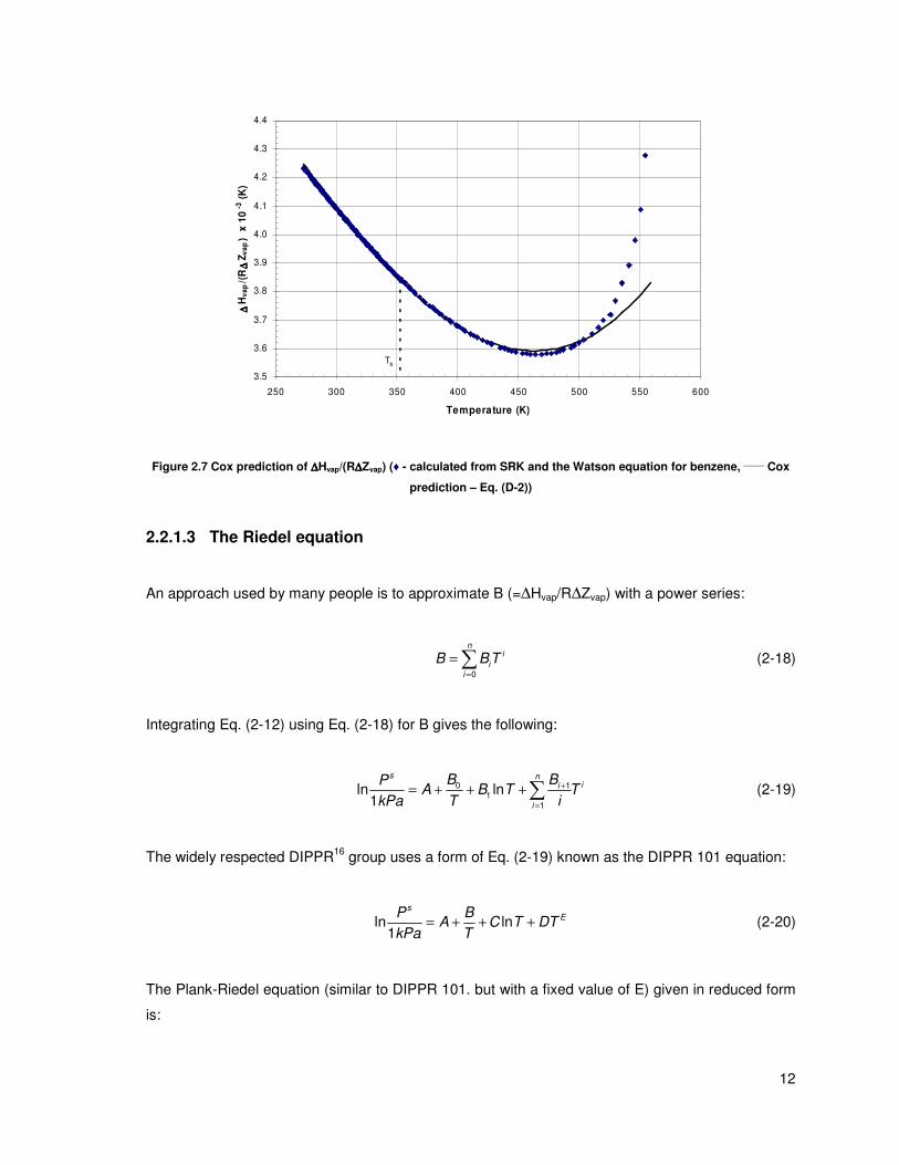
Figure 2.7 Cox prediction of ∆Hvap/(R∆Zvap) (♦ - calculated from SRK and the Watson equation for

benzene, _____

Cox prediction – Eq. (D-2)) ........................................................................................ 12

Figure 2.8 Riedel prediction of ∆Hvap/(R∆Zvap) (♦ - data from SRK and the Watson equation for

benzene, _____

Riedel prediction – Eq. (D-3), - - - Riedel direct fit – Eq. (D-3))................................. 14

Figure 2.9 Best possible Mydral & Yalkowsky prediction of ∆Hvap/(R∆Zvap) (♦ - data from SRK and

the Watson equation for benzene, _____

Mydral & Yalkowsky prediction – Eq. (D-4))....................... 16

Figure 2.10 Best possible Tu prediction of ∆Hvap/(R∆Zvap) (♦ - data from SRK and the Watson

equation for benzene, _____

Tu prediction – Eq. (D-5)) ...................................................................... 18

Figure 2.11 Best possible “modified Watson” prediction of ∆Hvap/(R∆Zvap) (♦ - data from SRK and the

Watson equation for benzene, _____

“Modified Watson” prediction – Eq. (D-6))............................... 20

ix

Figure 2.12 Abrams et al. prediction of ∆Hvap/(R∆Zvap) (♦ - data from SRK and the Watson equation

for benzene, _____

Abrams et al. prediction – Eq. (D-7)) .................................................................... 22

Figure 2.13 SRK prediction of ∆Hvap/(R∆Zvap) (♦ - data from SRK and the Watson equation for

benzene, _____

SRK prediction – Appendix F) ................................................................................... 25

Figure 2.14 Lee-Kesler prediction of ∆Hvap/(R∆Zvap) (♦ - data from SRK and the Watson equation for

benzene, _____

Lee-Kesler prediction – Eq. (D-8)) ............................................................................. 27

Figure 2.15 Wagner prediction of ∆Hvap/(R∆Zvap) (♦ - data from SRK and the Watson equation for

benzene, _____

Wagner prediction – Eq. (D-9)).................................................................................. 29

Figure 2.16 ln(Ps/101.3kPa) vs. 1/T for benzene, with solid vapour pressure data (x – liquid data

taken from the DDB, x – solid data taken from the DDB ____

solid vapour pressure, - - - - sub cooled

liquid vapour pressure)...................................................................................................................... 32

Figure 3.1 Experimental data from the DDB for amyl formate.......................................................... 34

Figure 3.2 Experimental data from the DDB for n-eicosane ............................................................. 34

Figure 3.3 Flow diagram for the “Inside-Outside” regression technique........................................... 40

Figure 3.4 The group definition and structure of the aliphatic carboxylic acid group........................ 41

Figure 4.1 A proper fit for the Eq. (2-27) ........................................................................................... 43

Figure 4.2 A physically unrealistic fit for Eq. (2-27)........................................................................... 43

Figure 4.3 ln(Ps/1 kPa) vs. T for 1-butanol (♦ - data from the DDB,

_____ with the logarithm term, - - - -

without the logarithm term)................................................................................................................ 45

Figure 4.4 ∆Hvap/(R∆Zvap) for 1-butanol (♦ - data from SRK using the MC alpha function and the

Watson equation (Eq. (2-36) with m = 0.473), _____

prediction with the logarithm term, - - - -

prediction without the logarithm term)............................................................................................... 45

Figure 4.5 B’ vs. polarizability for the n-alkanes ............................................................................... 46

x

Figure 4.6 B’ vs. polarizability for hydrocarbons ............................................................................... 47

Figure 4.7 Tb vs. polarizability for hydrocarbons ............................................................................... 47

Figure 4.8 Comparison of the group contribution approaches for the non-cyclic alkene groups...... 49

Figure 5.1 ln(Ps/101.3kPa) vs. 1/T for propane (x – data taken from the DDB, - - - - data regressed

using the C-parameter correlation of Nannoolal et al., ______

data regressed using the improved C-

parameter correlation) ....................................................................................................................... 51

Figure 5.2 Ps vs. T for propane (x – data taken from the DDB, - - - - data regressed using the C-

parameter correlation of Nannoolal et al., ______

data regressed using the improved C-parameter

correlation) ........................................................................................................................................ 52

Figure 5.3 ln(Ps/101.3kPa) vs. 1/T for octadecane (x – data taken from the DDB, - - - - data

regressed using the C-parameter correlation of Nannoolal et al., ______

data regressed using the

improved C-parameter correlation) ................................................................................................... 52

Figure 5.4 Ps vs. T for octadecane (x – data taken from the DDB, - - - - data regressed using the C-

parameter correlation of Nannoolal et al., ______

data regressed using the improved C-parameter

correlation) ........................................................................................................................................ 53

Figure 5.5 Comparison of the properties of anthracene and phenanthrene. .................................... 53

Figure 5.6 dBi vs. number of atoms for different alkynes (♦ – dBi data for each compound, ____

a

linear least squares fit) ...................................................................................................................... 54

Figure 5.7 dBi vs. number of atoms for different alkenes (♦ – dBi data for each compound, ____

a


Figure 5.8 ln(Ps/101.3kPa) vs. 1/T for 1-nonanol (x – data taken from the DDB, - - - - data regressed

using the method of Nannoolal et al., ______

data regressed using the new logarithmic correction) 57

Figure 5.9 Ps vs. T for 1-nonanol (x – data taken from the DDB, - - - - data regressed using the

method of Nannoolal et al., ______

data regressed using the new logarithmic correction) ................ 57

xi

Figure 5.10 ln(Ps/101.3kPa) vs. 1/T for palmitic acid (x – data taken from the DDB, - - - - data

regressed using the method of Nannoolal et al., ______

data regressed using the new logarithmic

correction) ......................................................................................................................................... 58

Figure 5.11 Ps vs. T for palmitic (x – data taken from the DDB, - - - - data regressed using the

method of Nannoolal et al., ______

data regressed using the new logarithmic correction) ................ 58

Figure 5.12 dBi vs. number of atoms for different epoxides (♦ – dBi data for each compound, ____

a


Figure 5.13 dBi vs. number of atoms for different ketones (♦ – dBi data for each compound, ____

a


Figure 5.14 dBi vs. number of atoms for different aliphatic alcohols (♦ – dBi data for each

compound, ____

lines to show the trends) .......................................................................................... 60

Figure 5.15 dBi vs. number of atoms for different aliphatic carboxylic acids (♦ – dBi data for each

compound, ____

lines to show the trends) .......................................................................................... 61

Figure 5.16 GIj vs. number of atoms for different diols (♦ – dBi data for each compound, ____

a linear

least squares fit) ................................................................................................................................ 61

Figure 5.17 dBi vs. number of atoms for different primary aliphatic amines (♦ – dBi data for each

compound, ____

a linear least squares fit) .......................................................................................... 64

Figure 5.18 dBi vs. number of atoms for different nitriles (♦ – dBi data for each compound, ____

lines

to show the trends)............................................................................................................................ 64

Figure 5.19 dBi vs. number of atoms for different aliphatic isocyanates (♦ – dBi data for each

compound, ____

a linear least squares fit) .......................................................................................... 65

Figure 5.20 ln(Ps/101.3kPa) vs. 1/T for thymol (x – solid data taken from the DDB,

____ vapour

pressure curve) ................................................................................................................................. 71

Figure 5.21 ln(Ps/101.3kPa) vs. 1/T for diethyl malonate (x – data taken from the DDB,

____

predicted, - - - - fitted)........................................................................................................................ 74

xii

Figure 5.22 Histogram of the vapour pressure relative mean deviation for the compounds in the

training set......................................................................................................................................... 75

Appendices

Figure E.1 Screenshot of the GUI used to validate the data – this enabled the fast removal of any

obvious outliers ................................................................................................................................. 98

Figure E.2 Screenshot of the GUI used to test the different models – enabled the rapid testing of the

forms of the equation that were tested for this work ......................................................................... 99

Figure F.1 P vs. V for water at 560 K as given by the van der Waals EOS.................................... 101

Figure F.2 Heat of vaporization of benzene as a function of temperature (♦ – data from the DDB,

____ SRK prediction Eq. (F-13))........................................................................................................ 103

Figure F.3 Heat of vaporization of benzene as a function of temperature (♦ – data from the DDB,

____ Twu SRK prediction Eq.(F-14) and Eq. (F-9) in the form of Eq. (F-13)) ................................... 103

xiii

LIST OF TABLES

Table 2.1 Antoine constants for various temperature ranges ............................................................. 9

Table 2.2 Relative mean deviations (RMD) for vapour pressures of selected compounds – Antoine

equation............................................................................................................................................. 10

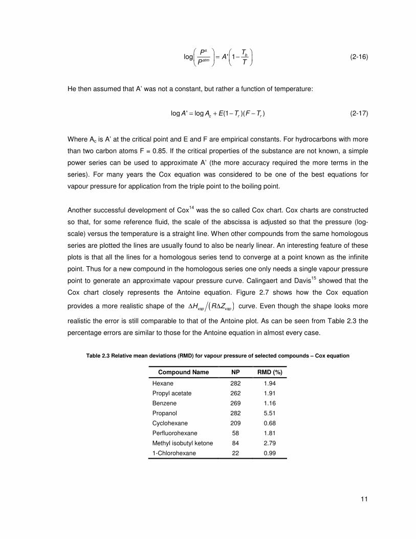
Table 2.3 Relative mean deviations (RMD) for vapour pressure of selected compounds – Cox

equation............................................................................................................................................. 11

Table 2.4 Relative mean deviations (RMD) for vapour pressure of selected compounds – Riedel

equation............................................................................................................................................. 13

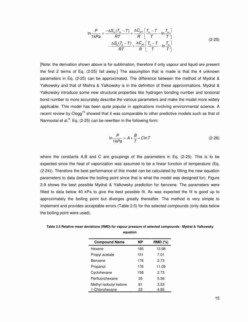
Table 2.5 Relative mean deviations (RMD) for vapour pressure of selected compounds - Mydral &

Yalkowsky equation........................................................................................................................... 15

Table 2.6 Relative mean deviations (RMD) for vapour pressure of selected compounds – Tu

equation............................................................................................................................................. 18

Table 2.7 Relative mean deviations (RMD) for vapour pressure of selected compounds – Eq. (2-38)

........................................................................................................................................................... 20

Table 2.8 Relative mean deviations (RMD) for vapour pressure of selected compounds – method of

Abrams et al ...................................................................................................................................... 22

Table 2.9 Relative mean deviations (RMD) for vapour pressure of selected compounds – SRK EOS

using Eqn. (2-48)............................................................................................................................... 25

Table 2.10 Relative mean deviations (RMD) for vapour pressure of selected compounds – Lee-

Kesler ................................................................................................................................................ 26

Table 2.11 Relative mean deviations (RMD) for vapour pressure of selected compounds – Wagner

(* - parameters fitted by author) ........................................................................................................ 29

Table 5.1 New hydrocarbon structural groups (Ink No – fragmentation group number, Ref No –

xiv

reference number is used to arrange like groups (e.g. halogen groups etc) since the ink no’s have

no real structure) ............................................................................................................................... 50

Table 5.2 Relative mean deviation [%] in vapour pressure estimation for different types of

hydrocarbons (this work). The number in superscript is the number of data points used; the main

number is the average percentage error of each data point. NC – Number of compounds; ELP –

Extremely low pressure P < 10 Pa; LP – Low pressure 10 Pa 500 kPa; AVE – Average error. ............................ 55

Table 5.3 Relative mean deviation [%] in vapour pressure estimation for different types of

hydrocarbons (Nannoolal et al.). The number in superscript is the number of data points used; the

main number is the average percentage error of each data point. NC – Number of compounds; ELP

– Extremely low pressure P < 10 Pa; LP – Low pressure 10 Pa 500 kPa; AVE – Average error. ............. 56

Table 5.4 Relative mean deviation [%] in vapour pressure estimation for different types of oxygen

containing compounds (this work). The number in superscript is the number of data points used; the




Table 5.5 Relative mean deviation [%] in vapour pressure estimation for different types of oxygen

containing compounds (Nannoolal et al.). The number in superscript is the number of data points

used; the main number is the average percentage error of each data point. NC – Number of

compounds; ELP – Extremely low pressure P < 10 Pa; LP – Low pressure 10 Pa 500 kPa; AVE – Average error.

........................................................................................................................................................... 63

Table 5.6 Relative mean deviation [%] in vapour pressure estimation for different types of nitrogen





Table 5.7 Relative mean deviation [%] in vapour pressure estimation for different types of nitrogen



xv



........................................................................................................................................................... 66

Table 5.8 Relative mean deviation [%] in vapour pressure estimation for different types of sulfur





Table 5.9 Relative mean deviation [%] in vapour pressure estimation for different types of sulfur





........................................................................................................................................................... 67

Table 5.10 Relative mean deviation [%] in vapour pressure estimation for different types of halogen





Table 5.11 Relative mean deviation [%] in vapour pressure estimation for different types of halogen





........................................................................................................................................................... 68

Table 5.12 Relative mean deviation [%] in vapour pressure estimation for various other compounds.

The number in superscript is the number of data points used; the main number is the average

percentage error of each data point. NC – Number of compounds; ELP – Extremely low pressure P

< 10 Pa; LP – Low pressure 10 Pa 500 kPa; AVE – Average error......................................................................... 69

xvi

Table 5.13 Relative mean deviation [%] in vapour pressure estimation for various other compounds

(Nannoolal et al.). The number in superscript is the number of data points used; the main number is

the average percentage error of each data point. NC – Number of compounds; ELP – Extremely

low pressure P < 10 Pa; LP – Low pressure 10 Pa 500 kPa; AVE – Average error............................................. 69

Table 5.14 Percentage errors for the test set data ........................................................................... 70

Table 5.15 Percentage errors for heat of vaporization at 298.15 K using Eq. (5-2) with ∆Z = 1 ...... 72

Table 5.16 Results for the prediction of Hildebrand solubility parameters at 298 K ......................... 73

Table 5.17 Relative mean deviation [%] in vapour pressure estimation for the new method and the

method of Nannoolal et al. The number in superscript is the number of data points used; the main

number is the average percentage error of each data point. NC – Number of compounds; ELP –

Extremely low pressure P < 10 Pa; LP – Low pressure 10 Pa 500 kPa; AVE – Average error. ............................ 74

Appendices

Table A.1 Group contribution and group interaction values and descriptions .................................. 84

Table A.2 Group contribution values for the logarithmic correction term.......................................... 93

Table B.1 Calculation for the vapour pressure of 1-hexen-3-ol at 389K........................................... 94

Table B.2 Calculation for the vapour pressure of 2-mercapto ethanol at 364.8 K............................ 95

Table D.1 Forms of the equations for ∆H/R∆Z for the various equations used in this dissertation .. 97

xvii

NOMENCLATURE

a, b, c, d - model parameters/constants

A,B,C,D,E - model parameters/constants

B’,D’ - parameters predicted by group contribution

Cp - constant pressure heat capacity (J/mol.K)

G - Gibbs free energy (J/mol)

H - enthalpy (J/mol)

M - molar mass (g/mol)

n - number of moles

P - pressure (kPa)

R - ideal gas constant (J/mol.K)

S - entropy (J/mol.K)

T - absolute temperature (K)

V - molar volume (cm3/mol)

Z - compressibility factor

Greek symbols

µ - chemical potential

ω - Pitzer acentric factor

xviii

Subscripts

atm - atmospheric

b - normal boiling point

c - critical point

m - normal melting point

r - reduced property

vap - vaporization

Superscripts

s - saturated / solid

l - liquid

v - vapour

__________________________________________

All other symbols used are explained in the text and unless otherwise stated SI units have been

used.

1

1 INTRODUCTION

Vapour pressure has for a long time been an important property in chemical and engineering

applications. It is useful in the design of distillation columns, storage and transport of materials and

for determining cavitation in pumps to name a few examples. It is also important for predicting the

fate of chemicals in the environment due to its predominant effect on the distribution coefficient

between air and various other compartments (e.g. air and water). Daubert1 ranked vapour pressure

second, behind critical properties, in the list of the most important thermophysical properties

(ranking is based on required accuracy and uses).

Many fitted (i.e. fitted directly to data) and predictive methods are available for the representation of

the vapour pressure curve. Correlated (or fitted) methods are usually good over the range of data

fitted but some extrapolate very poorly if not fitted to a wide enough data range (some of these

methods will be discussed in the following chapters). A drawback of fitted models is that their

parameters require experimental data which in many cases are not available. This means that a

suitable quantity of the chemical (if not readily available) must be synthesized and vapour pressure

measurements undertaken.

Even though the Dortmund Data Bank (DDB2) contains over 180 000 data points for more than

6000 compounds, it is only a fraction of the more than 100 000 (according to the environmental

news network3) chemicals that are reported to be in use today. This coupled with the fact that new

chemicals are continually being discovered (Bowen et al.4 estimate 200 to 1000 chemicals per

annum) means that measurement is not only very expensive but also impractical (even though

there is such a large amount of chemicals being discovered per annum many of these chemicals

have vapour pressure which is too low to be of practical concern). For this reason accurate

prediction methods have become increasingly popular.

A popular approach for the prediction of thermophysical properties is group contribution methods.

The component is broken down into structural groups (e.g. CH3, OH etc.). Their contributions are

combined to describe the behaviour of the whole molecule. The methods are especially popular for

properties like boiling point and critical properties, but surprisingly few exist (or are published) for

vapour pressure prediction.

In the preceding work of Rarey et al.5 and Nannoolal et al.

6,7,8, group contribution estimation

methods for the normal boiling point, critical data and vapour pressure of organic non-electrolyte

compounds were presented. The objective of this work is to extend and improve the method for

2

vapour pressure estimation. This was achieved by addition of more data to the training set, further

critical examination of the training set data and extended utilization of low pressure data for higher

molecular weight components. Structural and functional groups were defined in such a way as to

make the method as widely applicable as possible. Due to the importance of vapour pressure data

the predictions should be reasonably accurate (usually within 5%) and have a low probability of total

failure (i.e. errors in excess of 15%).

3

2 THEORY AND LITERATURE REVIEW

2.1 Introduction

By adding or removing heat from a pure substance or changing the system pressure, one can

change the phase of the substance. Some of the common phase transitions are as follows:

sublimation deposition

melting freezing

condensation vaporization

Solid Gas Solid

Solid Liquid Solid

Gas Liquid Gas

→ →

→ →

→ →

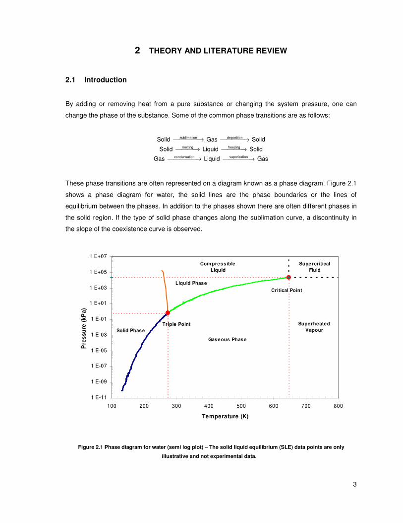
These phase transitions are often represented on a diagram known as a phase diagram. Figure 2.1

shows a phase diagram for water, the solid lines are the phase boundaries or the lines of

equilibrium between the phases. In addition to the phases shown there are often different phases in

the solid region. If the type of solid phase changes along the sublimation curve, a discontinuity in

the slope of the coexistence curve is observed.

Triple Point

Critical Point

1 E-11

1 E-09

1 E-07

1 E-05

1 E-03

1 E-01

1 E+01

1 E+03

1 E+05

1 E+07

100 200 300 400 500 600 700 800

Temperature (K)

Pre

ss

ure

(k

Pa

)

Gaseous Phase

Liquid Phase

Superheated

Vapour

Com press ible

Liquid

Supercritical

Fluid

Solid Phase

Figure 2.1 Phase diagram for water (semi log plot) – The solid liquid equilibrium (SLE) data points are only

illustrative and not experimental data.

4

The lines of equilibrium show where 2 phases coexist, and the triple point is where

solid/liquid/vapour all coexist. Consider a liquid in a sealed container with a vapour space above the

liquid; the molecules in the vapour phase will eventually reach a state of dynamic equilibrium, with

the rate of vaporization being equal to the rate of condensation. The vapour space is then said to be

saturated and the resulting pressure in the container is called the saturated vapour pressure.

The boiling point of a substance is defined as the temperature at which the saturated vapour

pressure is equal to the ambient pressure. The most common vapour pressure point is the normal

boiling point, it is the temperature at which the saturated vapour pressure is 1 atm (this is known as

the standard atmospheric pressure and is defined to be 101.325 kPa).

Due to its importance in process simulation (specifically distillation), vapour pressure is regarded as

one of the most important thermophysical properties. Daubert1 ranks vapour pressure as the

second most important thermophysical property, whereby his ranking system is based on the use of

the property on its own, its input into other equations and the accuracy to which the property should

be known. Unsurprisingly critical properties were ranked number one mainly due to the large

number of corresponding states methods and correlations that are based on this reference point

(many of the more accurate vapour pressure correlations also use critical data).

Many equations have been developed to describe the vapour pressure from the triple point to the

critical point. The Wagner9 equation has been shown to be able to reproduce the curve but it

requires knowledge of the critical point and accurate data. Therefore an equation is required which

gives the correct behaviour where only few data are available. Many of the vapour pressure

equations that are used in industry today have their roots in the Clausius-Clapeyron equation.

2.2 Vapour pressure models

2.2.1 Classical thermodynamics

A thermodynamic treatment of the pure component phase equilibrium described above was

presented by Gibbs and further refined by other researchers (esp. Riedel, Ambrose). Gibbs

introduced a quantity known as the chemical potential. The chemical potential of a species i, is

given by the change in the total Gibbs free energy of a system if one mole (or molecule) of this

species is removed or added. This process must not alter the state of the system, therefore the

chemical potential is defined as:

5

, , j i

i

i T P n

G

nµ

≠

∂=

∂ (2-1)

At a particular temperature and pressure the phase which has the lower chemical potential will be

the more stable phase. Taking the example of the container used above, if the temperature of the

liquid is suddenly raised the following will result (see Appendix G):

v lµ µ< (2-2)

This means that there will be transfer of mass from the liquid to the vapour phase until the chemical

potentials in both phases are equal. Therefore for all points on the equilibrium curve the following

holds (α and β represent the 2 phases on the curve):

α βµ µ= (2-3)

Since for a pure substance the chemical potential is only a function of and 2 of the 3 (there is no

composition) state variables, we chose T and P (since we want an expression for vapour pressure)

and take the total differential of both sides of Eq. (2-3) is:

P T P T

dT dP dT dPT P T P

α α β βµ µ µ µ ∂ ∂ ∂ ∂+ = +

∂ ∂ ∂ ∂ (2-4)

The differential form of the Gibbs function is (G,S and V are all molar properties):

dG SdT VdP= − + (2-5)

Eq. (2-5) has the same form as Eq. (2-4) and since G µ= (for a pure substance) the following two

expressions arise:

i

i

T

VP

µ ∂=

∂ (2-6)

i

i

P

ST

µ ∂= −

∂ (2-7)

6

Substituting Eq. (2-6) and Eq. (2-7) into Eq. (2-4) yields:

S dT V dP S dT V dPα α β β− + = − + (2-8)

This can be rewritten as:

dP S S

dT V V

α β

α β

−=

− (2-9)

Since the two phases are in equilibrium, Eq. (2-10) holds and substituting this into Eq. (2-9) yields

Eq.(2-11):

H H

S ST

α βα β −

− = (2-10)

( )

dP H H H

dT T VT V V

α β

α β

− ∆= =

∆− (2-11)

Eq. (2-11) is the well known Clausius-Clapeyron equation and it is valid for all points along the lines

of coexistence. As stated above, it is frequently used as the starting point for vapour pressure

correlations. A popular form of Eq. (2-11) is obtained by substituting the compressibility factor for

the molar volume, and tidying up the differential on the left hand side:

ln

1

d P H

R Zd

T

∆= −

∆

(2-12)

As shown is Figures 2.2 and 2.3 both ∆Hvap and ∆Zvap are similar functions of temperature. For this

reason the simplest assumption that can be made is that the LHS of Eq. (2-12) is a constant, for the

sake of simplicity, called B. Integration of Eq. (2-12) is then trivial:

ln1

P BA

kPa T= − (2-13)

This expression can be surprisingly accurate for small enough temperature ranges (typically <20 K,

however for certain parts of the temperature range can be as large as 60 K – see Figure 2.4) but for

larger temperature ranges it is woefully inaccurate. For this reason various modifications have

7

been made to increase the accuracy of the predictions. The two most well known of the semi-

empirical (Clausius-Clapeyron) type equations are those of Antoine10

and Riedel11

. These two

methods and others will be discussed in the sections following.

0

5

10

15

20

25

30

35

40

250 300 350 400 450 500 550 600

Temperature (K)

∆∆ ∆∆H

va

p (

kJ

/mo

l)

Figure 2.2 Heat of vaporization of benzene as a function of temperature (♦ – data from the DDB2,

____ Watson

equation [Eq. (2-36) with m = 0.391])

0.20

0.30

0.40

0.50

0.60

0.70

0.80

0.90

1.00

250 300 350 400 450 500 550 600

Temperature (K)

∆∆ ∆∆Z

va

p

Figure 2.3 ∆∆∆∆Zvap of benzene as a function of temperature using the SRK EOS with Twu alpha function (Twu et al.12

)

8

29

30

31

32

33

34

35

36

0.45 0.55 0.65 0.75 0.85 0.95

Tr

∆∆ ∆∆H

va

p/ ∆∆ ∆∆

Zv

ap

(k

J/m

ol)

Figure 2.4 ∆∆∆∆Hvap/∆∆∆∆Zvap of benzene as a function of reduced temperature (Tr = T/Tc) (calculated from the Watson and

the SRK EOS using the Twu alpha function (Twu et al.12

))

Figure 2.4 shows why the assumption of B being a constant is a poor one (except 0.76 < Tr < 0.86),

however is quite evident that the curve is more or less linear below the boiling point (Tr ≈ 0.63).

2.2.1.1 The Antoine equation

The main problem with Eq. (2-13) is that it is based on assumptions which do not hold. Thus further

corrections had to be developed to make the equation more widely applicable. Antoine10

proposed

a new form of Eq. (2-13) as:

log1

sP BA

kPa T C= +

− (2-14)

The introduction of the C parameter meant that the equation could now account for the slight

bowing of the vapour pressure curve. This equation has since become known as the Antoine

equation and has become very popular due to its simplicity and accuracy. The Antoine equation can

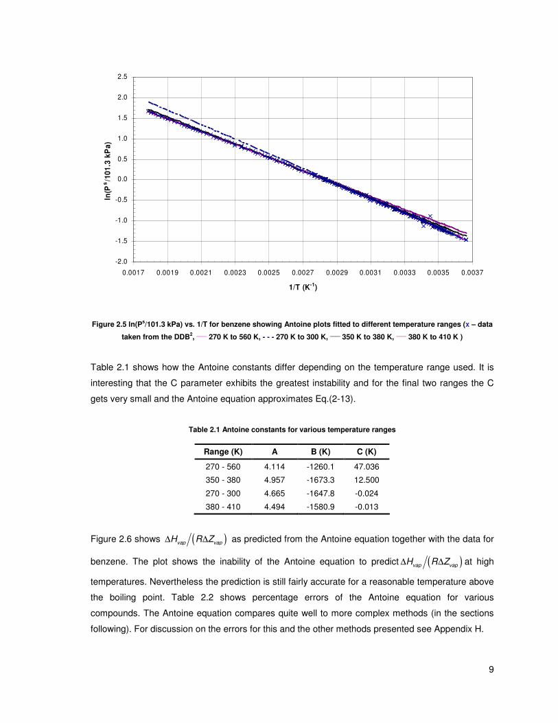
suffer from poor extrapolation (as with most other fitted models) as shown in Figure 2.5. The

equation which was fitted over the full range (270 K – 560 K) of data shows good correlation, even

the fairly narrow mid-range data (350 K – 380 K) shows fairly good extrapolation either way. The

problem is that when the equation is regressed against either low or high pressure data the

extrapolation tends to be fairly poor.

9

-2.0

-1.5

-1.0

-0.5

0.0

0.5

1.0

1.5

2.0

2.5

0.0017 0.0019 0.0021 0.0023 0.0025 0.0027 0.0029 0.0031 0.0033 0.0035 0.0037

1/T (K-1)

ln(P

s/1

01

.3 k

Pa

)

Figure 2.5 ln(Ps/101.3 kPa) vs. 1/T for benzene showing Antoine plots fitted to different temperature ranges (x – data

taken from the DDB2,

____ 270 K to 560 K, - - - 270 K to 300 K,

____ 350 K to 380 K,

____ 380 K to 410 K )

Table 2.1 shows how the Antoine constants differ depending on the temperature range used. It is

interesting that the C parameter exhibits the greatest instability and for the final two ranges the C

gets very small and the Antoine equation approximates Eq.(2-13).

Table 2.1 Antoine constants for various temperature ranges

Range (K) A B (K) C (K)

270 - 560 4.114 -1260.1 47.036

350 - 380 4.957 -1673.3 12.500

270 - 300 4.665 -1647.8 -0.024

380 - 410 4.494 -1580.9 -0.013

Figure 2.6 shows ( )vap vapH R Z∆ ∆ as predicted from the Antoine equation together with the data for

benzene. The plot shows the inability of the Antoine equation to predict ( )vap vapH R Z∆ ∆ at high

temperatures. Nevertheless the prediction is still fairly accurate for a reasonable temperature above

the boiling point. Table 2.2 shows percentage errors of the Antoine equation for various

compounds. The Antoine equation compares quite well to more complex methods (in the sections

following). For discussion on the errors for this and the other methods presented see Appendix H.

10

Table 2.2 Relative mean deviations (RMD) for vapour pressures of selected compounds – Antoine equation

Compound Name NP RMD (%)

Hexane 282 2.34

Propyl acetate 262 1.68

Benzene 269 1.35

Propanol 282 5.03

Cyclohexane 209 0.87

Perfluorohexane 58 1.94

Methyl isobutyl ketone 84 3.29

1-Chlorohexane 22 1.12

3.5

3.6

3.7

3.8

3.9

4.0

4.1

4.2

4.3

4.4

250 300 350 400 450 500 550 600

Temperature (K)

∆∆ ∆∆H

va

p/(

R∆∆ ∆∆

Zv

ap

) x

10

-3 (K

)

Tb

Figure 2.6 Antoine prediction of ∆∆∆∆Hvap/(R∆∆∆∆Zvap) (♦ - calculated from SRK and the Watson equation for benzene, _____

Antoine prediction – Eq. (D-1))

2.2.1.2 The Cox equation and Cox charts

The approach taken by Cox13

was to rewrite Eq. (2-13) as follows:

log 's

atm

P BA

TP

= +

(2-15)

This means that at the normal boiling point the logarithm will fall away and therefore ' bB A T= − ,

which when substituted back into (2-15) yields:

11

log ' 1s

b

atm

TPA

TP

= −

(2-16)

He then assumed that A’ was not a constant, but rather a function of temperature:

log ' log (1 )( )c r rA A E T F T= + − − (2-17)

Where Ac is A’ at the critical point and E and F are empirical constants. For hydrocarbons with more

than two carbon atoms F = 0.85. If the critical properties of the substance are not known, a simple

power series can be used to approximate A’ (the more accuracy required the more terms in the

series). For many years the Cox equation was considered to be one of the best equations for

vapour pressure for application from the triple point to the boiling point.

Another successful development of Cox14

was the so called Cox chart. Cox charts are constructed

so that, for some reference fluid, the scale of the abscissa is adjusted so that the pressure (log-

scale) versus the temperature is a straight line. When other compounds from the same homologous

series are plotted the lines are usually found to also be nearly linear. An interesting feature of these

plots is that all the lines for a homologous series tend to converge at a point known as the infinite

point. Thus for a new compound in the homologous series one only needs a single vapour pressure

point to generate an approximate vapour pressure curve. Calingaert and Davis15

showed that the

Cox chart closely represents the Antoine equation. Figure 2.7 shows how the Cox equation

provides a more realistic shape of the ( )vap vapH R Z∆ ∆ curve. Even though the shape looks more

realistic the error is still comparable to that of the Antoine plot. As can be seen from Table 2.3 the

percentage errors are similar to those for the Antoine equation in almost every case.

Table 2.3 Relative mean deviations (RMD) for vapour pressure of selected compounds – Cox equation


Hexane 282 1.94


Benzene 269 1.16

Propanol 282 5.51





12

3.5

3.6

3.7

3.8

3.9

4.0

4.1

4.2

4.3

4.4

250 300 350 400 450 500 550 600

Temperature (K)

∆∆ ∆∆H

va

p/(

R∆∆ ∆∆

Zv

ap

) x

10

-3 (K

)

Tb

Figure 2.7 Cox prediction of ∆∆∆∆Hvap/(R∆∆∆∆Zvap) (♦ - calculated from SRK and the Watson equation for benzene, _____

Cox

prediction – Eq. (D-2))

2.2.1.3 The Riedel equation

An approach used by many people is to approximate B (=∆Hvap/R∆Zvap) with a power series:

0

ni

ii

B BT=

=∑ (2-18)

Integrating Eq. (2-12) using Eq. (2-18) for B gives the following:

0 11

1

ln ln1

s nii

i

B BPA B T T

kPa T i+

=

= + + +∑ (2-19)

The widely respected DIPPR16

group uses a form of Eq. (2-19) known as the DIPPR 101 equation:

ln ln1

sEP B

A C T DTkPa T

= + + + (2-20)

The Plank-Riedel equation (similar to DIPPR 101. but with a fixed value of E) given in reduced form

is:

13

6ln lns

r r r

r

BP A C T DT

T= + + + (2-21)

Based on the Principle of Corresponding States, a criterion known as the Riedel criterion was

derived. The Riedel criterion is deduced from plots of α vs. Tr, where α is defined as:

(ln )

(ln )r

r

d P

d Tα = (2-22)

It states that 0r

ddT

α = when Tr = 1 (i.e. at the critical point). Using αc (which is the value of alpha

at the critical point) one can then estimate the values of the Riedel parameters (A,B,C&D). Riedel

developed a set of further criteria, which needed to be met in order to obtain a physically realistic

vapour pressure equation. (see Appendix C). Figure 2.8 illustrates that the Riedel equation shows a

much better reproduction of the experimental shape of the vapour pressure equation than the

Antoine equation. The reason that the curve is slightly removed from the data points is that the

Riedel equation parameters are calculated from set criteria so as to make the fit physically realistic.

Also shown on the plot is the fitted Riedel equation, this was found by using the calculated Riedel

parameters as a starting point and regressing the parameters. The resulting curve shows a near

perfect representation of the curve up to about 530 K (which is 30 K below the critical temperature).

The percentage error for the selected compounds is actually worse than the methods of Antoine

and Cox on most occasions. This is not due to the model itself but just the way the parameters are

calculated (they are calculated solely from the Riedel criterion and are not fitted to the data).

Table 2.4 Relative mean deviations (RMD) for vapour pressure of selected compounds – Riedel equation


Hexane 282 2.08


Benzene 269 1.99

Propanol 282 7.24





14

3.5

3.6

3.7

3.8

3.9

4.0

4.1

4.2

4.3

4.4

250 300 350 400 450 500 550 600

Temperature (K)

∆∆ ∆∆H

va

p/(

R∆∆ ∆∆

Zv

ap

) x

10

-3 (K

)

Tb

Figure 2.8 Riedel prediction of ∆∆∆∆Hvap/(R∆∆∆∆Zvap) (♦ - data from SRK and the Watson equation for benzene, _____

Riedel

prediction – Eq. (D-3), - - - Riedel direct fit – Eq. (D-3))

2.2.1.4 The Myrdal & Yalkowsky equation

The method of Mydral & Yalkowsky17

is a modification of the work of Mishra & Yalkowsky18

. The

method is only valid for temperatures below the normal boiling point (the lower the better) since in

the model it is assumed that the change in compressibility factor upon vaporization (∆Zvap) is unity.

The form of the Clausius-Clapeyron equation then takes the following form:

2

ln1

sP HdT

kPa RT

∆= ∫ (2-23)

The change in enthalpy is then described in terms of the vaporization of a solid (assuming that the

heat of vaporization is a linear function of temperature):

( )( ) ( )( )s l l g

m b p p m p p bH H H C C T T C C T T∆ = ∆ + ∆ + − − + − − (2-24)

Then assuming that the heat capacities are constant with respect to temperature (which is a

reasonable assumption); integrating Eq. (2-23) and introducing the entropy of melting

( /m m mS H T∆ = ∆ ) and boiling ( /b b bS H T∆ = ∆ ) the following expression is obtained:

15

( )ln ln

1

( )ln

pmm m m m

pbb b b b

CS T T T T TP

kPa RT R T T

CS T T T T T

RT R T T

∆−∆ − − = + −

∆∆ − − − + −

(2-25)

[Note: the derivation shown above is for sublimation, therefore if only vapour and liquid are present

the first 2 terms of Eq. (2-25) fall away.] The assumption that is made is that the 4 unknown

parameters in Eq. (2-25) can be approximated. The difference between the method of Mydral &

Yalkowsky and that of Mishra & Yalkowsky is in the definition of these approximations. Mydral &

Yalkowsky introduce some new structural properties like hydrogen bonding number and torsional

bond number to more accurately describe the various parameters and make the model more widely

applicable. This model has been quite popular in applications involving environmental science. A

recent review by Clegg19

showed that it was comparable to other predictive models such as that of

Nannoolal et al.8. Eq. (2-25) can be rewritten in the following form:

ln ln1

P BA C T

kPa T= + + (2-26)

where the constants A,B and C are groupings of the parameters in Eq. (2-25). This is to be

expected since the heat of vaporization was assumed to be a linear function of temperature (Eq.

(2-24)). Therefore the best performance of this model can be calculated by fitting the new equation

parameters to data (below the boiling point since that is what the model was designed for). Figure

2.9 shows the best possible Mydral & Yalkowsky prediction for benzene. The parameters were

fitted to data below 40 kPa to give the best possible fit. As was expected the fit is good up to

approximately the boiling point but diverges greatly thereafter. The method is very simple to

implement and provides acceptable errors (Table 2.5) for the selected compounds (only data below

the boiling point were used).

Table 2.5 Relative mean deviations (RMD) for vapour pressure of selected compounds - Mydral & Yalkowsky

equation


Hexane 185 13.98


Benzene 176 2.73

Propanol 176 11.09





16

3.5

3.6

3.7

3.8

3.9

4.0

4.1

4.2

4.3

4.4

250 300 350 400 450 500 550 600

Temperature (K)

∆∆ ∆∆H

va

p/(

R∆∆ ∆∆

Zv

ap

) x

10

-3 (K

)

Tb

Figure 2.9 Best possible Mydral & Yalkowsky prediction of ∆∆∆∆Hvap/(R∆∆∆∆Zvap) (♦ - data from SRK and the Watson


Mydral & Yalkowsky prediction – Eq. (D-4))

2.2.1.5 The Tu group contribution method

A group contribution method for the estimation of vapour pressures was developed by Tu20

.

Assuming a quadratic temperature dependence of the B parameter the following vapour pressure

equation results (from the integration of the Clausius-Clapeyron):

ln ln1

sP BA C T DT

kPa T= + − − (2-27)

Then by the usual assumption that the total group contribution is simply the sum of the individual

contributions (see paragraph 4.2):

ln ln1

ii i i i

i

BPN A C T DT

kPa T

= + − −

∑ (2-28)

It was found, however that this model did not follow the group contribution scheme and therefore

the following final equation was used as it followed group contribution much better:

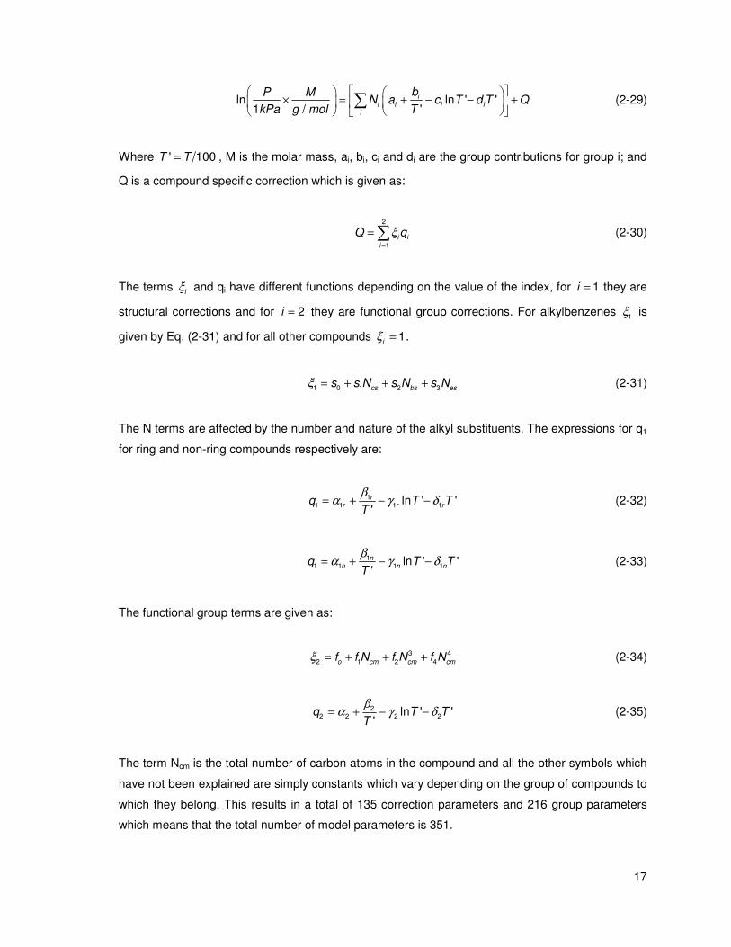
17

ln ln ' '1 / '

ii i i i

i

bP MN a c T d T Q

kPa g mol T

× = + − − +

∑ (2-29)

Where ' 100T T= , M is the molar mass, ai, bi, ci and di are the group contributions for group i; and

Q is a compound specific correction which is given as:

2

1i i

i

Q qξ=

= ∑ (2-30)

The terms iξ and qi have different functions depending on the value of the index, for 1i = they are

structural corrections and for 2i = they are functional group corrections. For alkylbenzenes 1ξ is

given by Eq. (2-31) and for all other compounds 1iξ = .

1 0 1 2 3cs bs ess s N s N s Nξ = + + + (2-31)

The N terms are affected by the number and nature of the alkyl substituents. The expressions for q1

for ring and non-ring compounds respectively are:

11 1 1 1ln ' '

'r

r r rq T TT

βα γ δ= + − − (2-32)

11 1 1 1ln ' '

'n

n n nq T TT

βα γ δ= + − − (2-33)

The functional group terms are given as:

3 4

2 1 2 4o cm cm cmf f N f N f Nξ = + + + (2-34)

22 2 2 2ln ' '

'q T T

T

βα γ δ= + − − (2-35)

The term Ncm is the total number of carbon atoms in the compound and all the other symbols which

have not been explained are simply constants which vary depending on the group of compounds to

which they belong. This results in a total of 135 correction parameters and 216 group parameters

which means that the total number of model parameters is 351.

18

The method is claimed to have an average deviation of 5% when tested with 336 organic

compounds with 5287 data points. The model parameters were generated by using a set containing

342 compounds with 5359 data points. The high number of model parameters makes this model

highly susceptible to over-fitting. Also since many of the parameters are “group-specific” the method

becomes less generally applicable. As with the model of Mydral & Yalkowsky the model of Tu was

tested by directly fitting Eq. (2-27) to the data and the resulting plot is shown in Figure 2.10. The

quadratic approximation increases the capability of the equation up to and just beyond the boiling

point but the model still falls off when nearing the critical point. The method of Tu is quite complex

to implement by hand and provides very poor prediction for some of the selected compounds.

Table 2.6 Relative mean deviations (RMD) for vapour pressure of selected compounds – Tu equation


Hexane 282 3.48


Benzene 269 19.40

Propanol 282 5.25


Perfluorohexane - -



3.5

3.6

3.7

3.8

3.9

4.0

4.1

4.2

4.3

4.4

250 300 350 400 450 500 550 600

Temperature (K)

∆∆ ∆∆H

va

p/(

R∆∆ ∆∆

Zv

ap

) x

10

-3 (K

)

Tb

Figure 2.10 Best possible Tu prediction of ∆∆∆∆Hvap/(R∆∆∆∆Zvap) (♦ - data from SRK and the Watson equation for benzene,

_____ Tu prediction – Eq. (D-5))

19

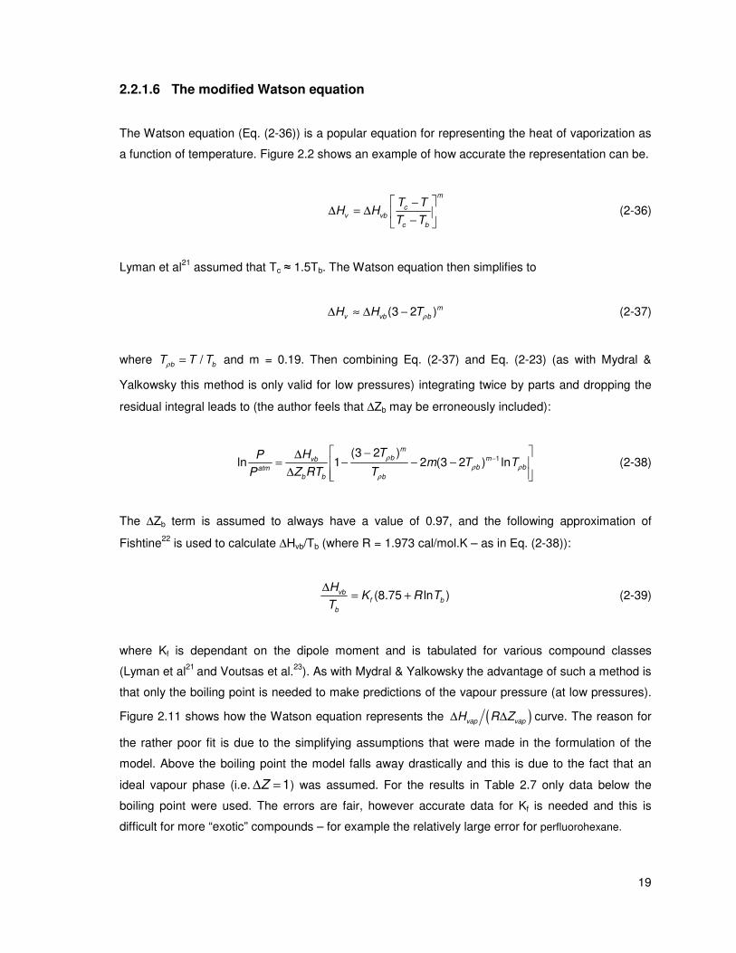
2.2.1.6 The modified Watson equation

The Watson equation (Eq. (2-36)) is a popular equation for representing the heat of vaporization as

a function of temperature. Figure 2.2 shows an example of how accurate the representation can be.

m

cv vb

c b

T TH H

T T

−∆ = ∆

− (2-36)

Lyman et al21

assumed that Tc ≈ 1.5Tb. The Watson equation then simplifies to

(3 2 )m

v vb bH H Tρ∆ ≈ ∆ − (2-37)

where /b bT T Tρ = and m = 0.19. Then combining Eq. (2-37) and Eq. (2-23) (as with Mydral &

Yalkowsky this method is only valid for low pressures) integrating twice by parts and dropping the

residual integral leads to (the author feels that ∆Zb may be erroneously included):

1(3 2 )

ln 1 2 (3 2 ) ln

m

b mvbb batm

b b b

THPm T T

Z RT TP

ρ

ρ ρ

ρ

− −∆

= − − − ∆

(2-38)

The ∆Zb term is assumed to always have a value of 0.97, and the following approximation of

Fishtine22

is used to calculate ∆Hvb/Tb (where R = 1.973 cal/mol.K – as in Eq. (2-38)):

(8.75 ln )vbf b

b

HK R T

T

∆= + (2-39)

where Kf is dependant on the dipole moment and is tabulated for various compound classes

(Lyman et al21

and Voutsas et al.23

). As with Mydral & Yalkowsky the advantage of such a method is

that only the boiling point is needed to make predictions of the vapour pressure (at low pressures).

Figure 2.11 shows how the Watson equation represents the ( )vap vapH R Z∆ ∆ curve. The reason for

the rather poor fit is due to the simplifying assumptions that were made in the formulation of the

model. Above the boiling point the model falls away drastically and this is due to the fact that an

ideal vapour phase (i.e. 1Z∆ = ) was assumed. For the results in Table 2.7 only data below the

boiling point were used. The errors are fair, however accurate data for Kf is needed and this is

difficult for more “exotic” compounds – for example the relatively large error for perfluorohexane.

20

Table 2.7 Relative mean deviations (RMD) for vapour pressure of selected compounds – Eq. (2-38)


Hexane 185 4.37


Benzene 176 5.89

Propanol 176 8.08





3.5

3.6

3.7

3.8

3.9

4.0

4.1

4.2

4.3

4.4

250 300 350 400 450 500 550 600

Temperature (K)

∆∆ ∆∆H

va

p/(

R∆∆ ∆∆

Zv

ap

) x

10

-3 (K

)

Tb

Figure 2.11 Best possible “modified Watson” prediction of ∆∆∆∆Hvap/(R∆∆∆∆Zvap) (♦ - data from SRK and the Watson


“Modified Watson” prediction – Eq. (D-6))

2.2.2 Kinetic theory of vaporization

According to kinetic theory, a gas is composed of a large number of molecules which when

compared to the distance between them are usually rather small. The molecules are in a constant

state of random motion and frequently collide with other molecules and any surrounding objects (i.e.

a container wall). The molecules are assumed to have standard physical properties (e.g. mass).

The average kinetic energy of the molecules (viz velocity) is a measure of the temperature of the

gas. Since the particles have mass the collisions with the gas and a surrounding container impart a

certain momentum on the container and gives rise to a pressure.

21

Abrams et al24

developed a vapour pressure equation based on the theoretical treatment of

Moelwyn-Hughes25

, which uses a multiple-oscillator model for the liquid phase, to take into account

for the form of the molecules (using a cubic approximation for B – see Eq. (2-13)):

2ln ln1

P BA C T DT ET

kPa T= + + + + (2-40)

The five parameters in the above equation are calculated directly from kinetic theory and so the

model has only two adjustable parameters. The first adjustable parameter is s, which is the number

of loosely coupled harmonic oscillators in each molecule (this is a model assumption). The second

parameter is the characteristic energy E0 which, together with temperature, is used to measure the

rate of molecules escaping into the vapour phase. The expressions for the five parameters are

given as follows (Γ(s) is the gamma function where Γ(s) = (s-1)!) :

[ ]0ln ( 0.5)ln ln ( ) lnw

ERA s s

V Rα

= + − − Γ +

(2-41)

0EB

R= − (2-42)

1.5C s= − (2-43)

0

1sD

E R

−= (2-44)

( )

2

0

2( 3)( 1)s sE

E R

− −= (2-45)

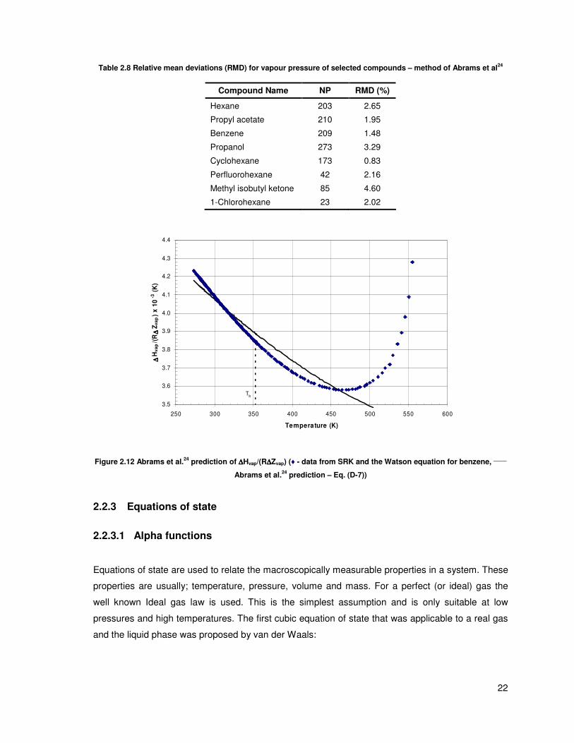
Figure 2.12 shows that this model describes ( )vap vapH R Z∆ ∆ fairly well. The model parameters given

by Abrams et al24

were inaccurate and therefore new values of E0 and s were fitted. The model was

only fitted to data below 200 kPa since that is the upper limit of the application of the model. Table

2.8 shows that the model performs very well for the test set of data with most predictions being in

the region of 2%. The power of this model is that it has all the benefits of a 5-parameter model

(good fit to data) and very few of the downfalls (i.e. stable fits to the data since there are only 2

adjustable parameters – see paragraph 4.1)

22

Table 2.8 Relative mean deviations (RMD) for vapour pressure of selected compounds – method of Abrams et al24


Hexane 203 2.65


Benzene 209 1.48

Propanol 273 3.29





3.5

3.6

3.7

3.8

3.9

4.0

4.1

4.2

4.3

4.4

250 300 350 400 450 500 550 600

Temperature (K)

∆∆ ∆∆H

va

p/(

R∆∆ ∆∆

Zv

ap

) x

10

-3 (K

)

Tb

Figure 2.12 Abrams et al.24

prediction of ∆∆∆∆Hvap/(R∆∆∆∆Zvap) (♦ - data from SRK and the Watson equation for benzene, _____

Abrams et al.24

prediction – Eq. (D-7))

2.2.3 Equations of state

2.2.3.1 Alpha functions

Equations of state are used to relate the macroscopically measurable properties in a system. These

properties are usually; temperature, pressure, volume and mass. For a perfect (or ideal) gas the

well known Ideal gas law is used. This is the simplest assumption and is only suitable at low

pressures and high temperatures. The first cubic equation of state that was applicable to a real gas

and the liquid phase was proposed by van der Waals:

23

( )2 m

m

aP V b RT

V

+ − =

(2-46)

Where Vm is the molar volume, a is the attraction parameter and b is the repulsion parameter.

These parameters are usually calculated from critical temperature and pressure. As cubic equations

of state (CEOS) predict identical behaviour for all fluid relative to their Tc and Pc, they are said to

employ the 2 parameter corresponding states principle. Since the equation of van der Waals many

CEOS have been developed for both pure components and mixtures in the vapour and liquid

phase. The most common type of EOS is the cubic EOS, cubic refers to the fact that if expanded

the equation would be at most a third order polynomial.

Many of the early equations of state had the downfall that they could not correlate the phase

equilibria of mixtures. Soave recognised that the performance for VLE (vapour-liquid-equilibria) was

not only dependant on the mixing rule (used to relate pure component parameters to mixture

parameters) but also on the performance with respect to pure component vapour pressures. This is

accounted for by use of the alpha function in the EOS, an example of such an EOS is the Soave-

Redlich-Kwong (SRK) EOS:

( )( , )r

m m m

a TRTP

V b V V b

α ω= −

− + (2-47)

As stated above the alpha function that enabled better vapour pressure representation (for non-

polar fluids) was suggested by Soave26

(there were other alpha-type functions that were developed

prior to this but they did not provide good enough vapour pressure representation):

0.5 2[1 (1 )]rm Tα = + − (2-48)

The parameter m is a function of acentric factor as follows (there are 2 versions of this equation):

20.480 1.574 0.175m ω ω= + − (2-49)

The Pitzer acentric factor for a pure compound is defined with reference to its vapour pressure. It

was noted that log rP against 1/ rT plots for simple fluids (Ar, Kr, Xe) lay on the same line and

passed through the point log 1.0 at T 0.7r rP = − = . The deviation of the non-simple fluids from this

point was defined as the acentric factor (Eq. (2-50)), which is sometimes thought of as a measure of

the non-sphericity of the molecule (with ω = 0 being perfectly spherical). Equations using the

24

parameter ω in addition to the Tc and Pc are said to employ the 3 parameter corresponding states

principle.

( )0.7

1.0 logr

r TPω

=≡ − − (2-50)

Soave’s alpha function was able reproduce vapour pressure at high reduced temperatures well but

diverged for low reduced temperature data (i.e. for the heavy hydrocarbons which have large critical

temperatures). There are many different forms of the alpha function that have been proposed since

Soave’s but, as noted by Coquelet et al.27

, they should satisfy the following criterion:

• They must be finite and positive at all temperatures

• They must be assume a value of 1 at the critical point

• The limit as temperature tends to infinity must be zero

• They must be continuous for T>0 as should their first and second derivatives

An example of a further developed alpha function is the 3-parameter Mathias-Copeman28

formulation (notice when c2 = c3 = 0 it has the same form as Eq. (2-48)):

( ) ( ) ( )22 3

1 2 3( , ) 1 1 1 1r r rT c T c T c Tα ω = + − + − + − (2-51)

The constants (c1-c3) can either be given as values or in the form of generalised equations similar to

Eq. (2-49). More recently a very successful alpha function was developed by Twu et al.12

(Eq.

(2-52)). In order to find reliable alpha function parameters that are also valid at very low pressure

the regression should include ideal gas and liquid heat capacity at low temperature.

( )( 1)( ) exp 1N M NM

r rT T L Tα − = − (2-52)

Vapour pressures can be found from the EOS by using the fact that l vφ φ= (since the phases are

in equilibrium) and solving the resulting equations for pressure (which will be the vapour pressure).

In the absence of a solver there is an iterative routine presented by Reid et al.29

. Table 2.9 shows

how the Soave EOS performs for the test set. The relatively high error for propanol is due to the fact

that this EOS is meant for non-polar molecules. The SRK plot for ( )vap vapH R Z∆ ∆ is shown in Figure

2.13 the prediction is remarkably good below the stationary point as apart from the critical

properties and the acentric factor no other data is needed. (The prediction of heat of vaporization is

25

shown in Appendix F, similar to the method of Eubank et al.30,31

).

Table 2.9 Relative mean deviations (RMD) for vapour pressure of selected compounds – SRK EOS using Eqn. (2-48)


Hexane 282 2.07


Benzene 269 1.69

Propanol 282 6.09





3.5

3.6

3.7

3.8

3.9

4.0

4.1

4.2

4.3

4.4

250 300 350 400 450 500 550 600

Temperature (K)

∆∆ ∆∆H

va

p/(

R∆∆ ∆∆

Zv

ap

) x

10

-3 (K

)

Tb

Figure 2.13 SRK prediction of ∆∆∆∆Hvap/(R∆∆∆∆Zvap) (♦ - data from SRK and the Watson equation for benzene, _____

SRK

prediction – Appendix F)

2.2.3.2 Lee-Kesler method

An alternative to the analytic approach of the cubic EOS is the 3 parameter corresponding states

method of Pitzer32

, which employs very precise data for two reference fluids. The linear interpolation

of Z with respect to 2 reference fluids as a function of the acentric factor is as follows:

(0) (1)( , ) ( , )r r r rZ Z T P Z T Pω= + (2-53)

26

The Z(0)

term is for simple fluids and the Z(1)

term is the departure function for a fluid with ω = 1. The

governing assumption is that fluids with the same acentric factor will have the same compressibility

factor. Once the compressibility factor is known it can be related to the state variables by its

definition:

PV

ZnRT

= (2-54)

The determination of the vapour pressure equation is similar to that of the compressibility factor,

with lnPr being a linear interpolation between 2 extreme cases:

(0) (1)ln ( ) ( )r r rP f T f Tω= + (2-55)

The functions f(0)

and f(1)

have are expressed by Lee and Kesler33,29

as follows (they have the same

form as the Riedel equation):

(0) 66.096485.92714 1.28862ln 0.169347r r

r

f T TT

= − − + (2-56)

(1) 615.687515.2518 13.4721ln 0.43577r r

r

f T TT

= − − + (2-57)

As with the alpha functions these equations are popular in the petroleum industry but are limited to

fluids for which critical data are available. The Lee-Kesler method was simple to implement and was

quite accurate for the set of test data (Table 2.10).

Table 2.10 Relative mean deviations (RMD) for vapour pressure of selected compounds – Lee-Kesler


Hexane 282 2.49


Benzene 269 1.62

Propanol 282 5.98





27

3.5

3.6

3.7

3.8

3.9

4.0

4.1

4.2

4.3

4.4

250 300 350 400 450 500 550 600

Temperature (K)

∆∆ ∆∆H

va

p/(

R∆∆ ∆∆

Zv

ap

) x

10

-3 (K

)

Tb

Figure 2.14 Lee-Kesler prediction of ∆∆∆∆Hvap/(R∆∆∆∆Zvap) (♦ - data from SRK and the Watson equation for benzene, _____

Lee-Kesler prediction – Eq. (D-8))

2.2.4 Empirical models

The very first vapour pressure equation was an empirical correlation suggested by Dalton34

(Eq.

(2-58)), however as more accurate vapour measurements were made available his prediction was

soon proven to be inaccurate.

ln '' ''1

PA B T

kPa= + (2-58)

Since then many empirical models have been developed for the prediction of the vapour pressure.

Another early empirical model is the one developed by Bose34

:

2 3

ln1

P b d ea

kPa T T T= − + + (2-59)

The empirical models that have gained a large amount of respect (and use) are not the ones that

are fitted to vapour pressure data indiscriminately but rather those which are subject to certain

constraints to make the curve physically realistic.

28

2.2.4.1 The Wagner equation

Arguably the most popular and widely used empirical method is that proposed by Wagner9,35

.

Originally the method was developed with very high precision data that was available (i.e. water,

nitrogen etc), however since then it has been applied to lower accuracy data. A common form of the

Wagner equation is as shown (sometimes referred to as the 1-1.5-3-6 Wagner or just the 3-6

Wagner equation):

1.5 3 6

ln1

r

a b c dP

τ τ τ τ

τ

+ + +=

− (2-60)

with the reversed temperature ( )1 rTτ = − . Fitting of the parameters of the Wagner equation is not

simply done by a least squared fit but rather by a more statistical approach where the equation is

subject to the following three constraints (as outlined by Chase36

):

• The resulting ∆Hvap/∆Zvap vs. T curve has a minimum within a specified range of reduced

temperature values (this is referred to as Waring’s37

criterion)

• At low reduced temperatures the value of ∆Hvap/∆Zvap should approximate ∆Hvap (This is

because at low reduced temperatures ∆Zvap → 1)

• The term ( )0.95

ln 'rT

P P=

must fall within a specified range, lnP’ is the straight line joining the

points Tr=0.7 and Tr=1 on a lnP vs 1/T plot (This is known as the Ambrose criterion)

The Wagner equation is widely used in industry for the purpose of simulation since it is one of the

few equations that can accurately represent the vapour pressure curve from the triple to the critical

point. As with the equations of state it can only be applied to compounds for which critical data are

available. As previously the validity of the model was analysed by plotting data for ∆Hvap/(R∆Zvap)

against the values predicted from the Wagner equation. The parameters for the Wagner equation

were obtained from Reid et al.29

. As can be seen in Figure 2.15, the Wagner equation is both

accurate and physically realistic. This has a lot to do with the way in which the parameters are fitted

(as discussed above). The reason that the curve seems to deviate slightly from the data could be

because the Wagner parameters were obtained from an external source and could therefore have

been fitted to some lower quality data. Nevertheless it is still quite clear that the Wagner equation

provides a physically realistic shape. Even though the Wagner equation has in most cases the

lowest error for the test data (Table 2.11), it is still comparable to the other methods that have been

presented.

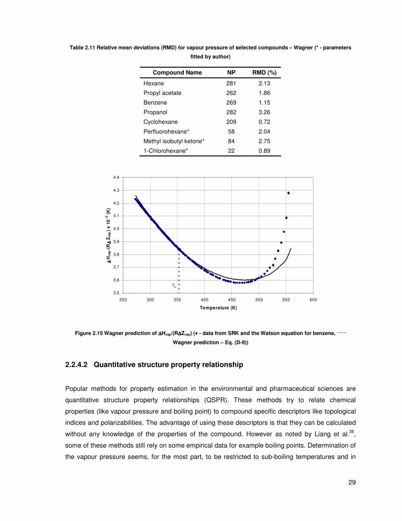
29

Table 2.11 Relative mean deviations (RMD) for vapour pressure of selected compounds – Wagner (* - parameters

fitted by author)


Hexane 281 2.13


Benzene 269 1.15

Propanol 282 3.26


Perfluorohexane* 58 2.04

Methyl isobutyl ketone* 84 2.75

1-Chlorohexane* 22 0.89

3.5

3.6

3.7

3.8

3.9

4.0

4.1

4.2

4.3

4.4

250 300 350 400 450 500 550 600

Temperature (K)

∆∆ ∆∆H

va

p/(

R∆∆ ∆∆

Zv

ap

) x

10

-3 (K

)

Tb

Figure 2.15 Wagner prediction of ∆∆∆∆Hvap/(R∆∆∆∆Zvap) (♦ - data from SRK and the Watson equation for benzene, _____

Wagner prediction – Eq. (D-9))

2.2.4.2 Quantitative structure property relationship

Popular methods for property estimation in the environmental and pharmaceutical sciences are

quantitative structure property relationships (QSPR). These methods try to relate chemical

properties (like vapour pressure and boiling point) to compound specific descriptors like topological

indices and polarizabilities. The advantage of using these descriptors is that they can be calculated

without any knowledge of the properties of the compound. However as noted by Liang et al.38

,

some of these methods still rely on some empirical data for example boiling points. Determination of

the vapour pressure seems, for the most part, to be restricted to sub-boiling temperatures and in

30

some cases to a single fixed temperature (usually 25°C).

A correlation that is proposed by Liang et al.38

, relies only on the polarizability and polar functional

group counts:

2

log 0.432 1.382( ) 0.482( ) 0.416( )1

2.197( ) 1.383( ) 1.101( ) 4.610

POH C O NH

kPa

COOH NO C N

α= − − − = − −

− − ≡ +

(2-61)

Where α is the polarizability and the bracketed terms refer to the number of the corresponding

functional group. The advantage of such an approach is that the vapour pressure can be calculated

from knowledge of the chemical structure (since the polarizability can be calculated using quantum

mechanical calculations). It is evident from the form of the equation that the vapour pressure is only

applicable to a single temperature (25°C in this case).

Another such model is proposed by Paul39

. The parameters in his equation are the solubility

parameter (SP), molar refractivity (MolRef), molecular weight (MW) and number of hydrogen

bonding acceptors (HBA). Both the solubility parameter and the molar refractivity can be calculated

from quantum mechanical calculations. The equation is again for 25°C and has the following form:

5 2log 8.81 0.2 5 10 ( )( )

1

0.05 Re 0.08

PHBA MW SP

kPa

Mol f SP

−= + − ×

− −

(2-62)

2.2.4.3 Interpolation polynomials

With the advent of computers, more complex mathematical approaches can be used for the

determination of the vapour pressure curve. One of the approaches that are used is to approximate

the vapour pressure curve with a very large polynomial series. This is useful because depending on

the accuracy needed; terms can be kept or dropped from the series. However this type of approach

is quite unstable as one further term can affect all the previously calculated values. Using

Chebyshev polynomials can make the equation more stable, this type of approach was outlined by

Ambrose40

.

A novel approach that was found is the use of Interpolation polynomials, where the interpolation

polynomial is fixed at certain points and a residual term accounts for any error in the resulting

expression. In the equation presented by Ledanois et al.41

Φ represents the interpolation polynomial

31

and Γ is the residue term:

ln ( ) ( )1

r r

PT T

kPa= Φ + Γ (2-63)

The general form of the interpolation polynomial (in the Newton form) and the residue are:

11

;

0 0 ;

;

ln 1 1( )

11

ini r

ri j r j r

i r

PT

T T

T

−−

= =

Φ = −

−∑ ∏ (2-64)

01 ;

1 1( )

n mi

r i rij r j r

T c TT T ==

Γ = −

∑∏ (2-65)

The indices n and m in the above equations refer to the number of ‘anchor points’ and the number

of parameters used in the residue function respectively. An approach of this type is useful

especially if there are good data available over the full vapour pressure range. It is most often

employed together with multi-parameter equations of state, where the solution of the iso-fugacity

criterion is numerically difficult. Instead the solutions for the vapour pressure curve are then

provided as Chebyshev polynomials for convenience.

2.3 Solvation theory

A method which has gained increasing popularity in recent times is predicting properties from

solvation theory. The great advantage of these methods is that they have the potential to be able to

produce results for any compound. The exact details of the quantum mechanical calculations are

beyond the scope of this work but the general procedure is to calculate the salvation free energy

(∆G*sol

) and relate this to the property of interest. Ben-Naim42

defines solvation as “The process of

transferring one molecule from a fixed position in an ideal gas phase to a fixed position in the fluid

phase at constant temperature and pressure”. An example of such a model is the one presented by

Lin et al.43

where they determine the solvation free energy as follows:

* * *

/ / /

sol vdw el

i i i i i iG G G∆ = ∆ + ∆ (2-66)

Where the vdw solvation free energy is in effect the non-polar (or van der Waals) contribution to the

salvation free energy and the el solvation free energy is made up of the polar and the hydrogen

32

bonding contributions. Lin et al.43

report a percentage error of 76% for vapour pressures at the

normal boiling point which shows that, while promising, these methods still have a long way to go to

compete with the current methods available.

2.4 Solid vapour pressures

Many high boiling organic compounds are solid at room temperature (and above). These

compounds exert a certain vapour pressure which is of particular interest to environmental

scientists who use it to determine the fate of compounds (there are many other uses). Solid vapour

pressure data can be converted to a sub cooled liquid vapour pressure which can be represented

using the models above. The conversion from solid to sub-cooled liquid data is shown in Figure

2.16. Since the difference between the gradients of the sub-cooled liquid line and the sublimation

line is known the conversion is a simple matter. The mathematical representation of this relationship

is given by:

1 1

ln ln1 1

sl m

m

PP H

kPa kPa R T T

∆= + −

(2-67)

Eq. (2-67) assumes that there are no further transition points (change from one solid phase to

another) and that the heat of melting is independent of the temperature which is often an

acceptable assumption as the heat capacity changes are relatively small.

-14

-12

-10

-8

-6

-4

-2

0

2

4

6

0.0015 0.002 0.0025 0.003 0.0035 0.004 0.0045 0.005 0.0055

1/T (K-1)

ln(P

s/1

01

.3 k

Pa

)

Figure 2.16 ln(Ps/101.3kPa) vs. 1/T for benzene, with solid vapour pressure data (x – liquid data taken from the DDB

2,

x – solid data taken from the DDB2 ____

solid vapour pressure, - - - - sub cooled liquid vapour pressure)

33

3 COMPUTATION AND DATABASE TOOLS

3.1 Database

The single factor which is most important for the development of a reliable model is the availability

of large amounts of accurate data. For this project the Dortmund Data Base (DDB) was utilized. The

DDB contains over 180 000 vapour pressure data points (both solid and liquid vapour pressures) for

some 6000 compounds.

All data were stored in a Microsoft Access database and Visual Basic for Applications (VBA) in

Excel was used to communicate with the database. VBA has many different means to communicate

with databases; a popular method is the use of ActiveX Data Objects (ADO). The basic steps that

VBA must use when accessing data via ADO are:

• Use ADO to establish a connection to the database

• Create a data storage variable (known as a record set)

• Populate the record set (e.g. via a structured query language (SQL) query)

• Analyse or manipulate the data and save any changes

• Close the record set and terminate the connection

3.2 Data validation

In order to make the model as generally applicable as possible the data that were used for

parameter regression needed to be accurate and free of outliers. Due to the massive amount of

data it was simply impractical to plot all the data manually and therefore a GUI (graphical user

interface) was developed in VBA in order to streamline the whole process. Plotting data is a very

good way of removing any obvious outliers, however due to the logarithmic scale high pressure

outliers were more difficult to notice. While plotting of the data is a very practical and fast way of

detecting outliers there is sometimes simply no way to determine the accuracy of the data. The

reason for this is that if there is only data from one source, the data may be smooth and therefore

seem accurate but may in fact have been measured incorrectly. (Screenshots of the data validation

GUI and the model testing GUI are shown in Appendix E)

Consider the following two typical examples of data found in the DDB. Figure 3.1 shows the plot of

the data for amyl formate. In the absence of any accurate boiling point data one may consider the

upper group of data to be the more accurate (as it contains the majority of the data points).

Fortunately in this example, the quality assessment in the DDB has marked the above data as

34

questionable and therefore they were removed from the training set. Typically this type of error

could be resolved by either the internal quality assessment of the DDB or the availability of accurate

boiling point data. Figure 3.2 shows the plot of the data for n-eicosane (C-20 alkane). There is a

large amount of scatter in the data with no real way to distinguish between good and poor data

(apart from some of the obvious outliers). For cases such as these data was either removed (for

use in the test dataset) or if the scatter was not too severe and the compound was “fairly exotic”

(i.e. contained unusual functional groups) it was included in the training set.

-5

-4

-3

-2

-1

0

1

0.0024 0.0025 0.0026 0.0027 0.0028 0.0029 0.003 0.0031 0.0032 0.0033 0.0034

1/T (K-1)

ln(P

s/1

01

.3 k

Pa

)

Figure 3.1 Experimental data from the DDB2 for amyl formate

-16

-14

-12

-10

-8

-6

-4

-2

0

2

0.0015 0.0017 0.0019 0.0021 0.0023 0.0025 0.0027 0.0029 0.0031 0.0033

1/T (K-1)

ln(P

s/1

01

.3 k

Pa

)

Figure 3.2 Experimental data from the DDB2 for n-eicosane

35

3.3 Regression

Since this project essentially entails model development, it is obvious that there is a certain amount

of “curve-fitting” required. The regression techniques described in the sections following are by no

means the only solution to parameter evaluation but are the ones that were thought to be most

suitable to the task. Both the linear and the non-linear routines were taken from the book by Press

et al.44

(only the algorithms and not the code).

3.3.1 Linear regression

The simplest case of regression is linear regression, whereby the model must be linear in the

parameters to be regressed as follows:

1

( ) ( )M

k kk

y x a X x=

=∑ (3-1)

The model does not have to be linear in x, since X(x) can be any function of x, for example the

following expression could result:

10 2( ) ln

ay x a a x

x= + + (3-2)

The next step is to define an objective function (sometimes called a merit function, F) which is a

measure of the deviation of the fitted model from the experimental data (yi):

2

1

1

( )M

i k k iNk

i i

y a X x

Fσ

=

=

−

=

∑∑ (3-3)

The term iσ is the standard deviation of the ith data point. From this point onwards it will be

disregarded (σi=1) since it was not used in this work.

We then define an N x M matrix A, and a vector b of length N as follows (N is number of data points

and M is number of parameters; for any meaningful results N > M):

36

( )ij j iA X x= (3-4)

i ib y= (3-5)

The “best-fit” occurs when the derivative of the objective function, with respect to the regression

parameters, falls to zero, therefore:

1 1

2 ( ) ( ) 0N M

k i i j j ii jk

FX x y a X x

a = =

∂= − − =

∂ ∑ ∑ (3-6)

Interchanging the order of the summations, simplifying and rearranging yields:

1

M

kj j kj

aα β=

=∑ (3-7)

where the expressions for α and β, in matrix form, are as follows:

[ ] Tα = ⋅A A (3-8)

{ } Tβ = ⋅A b (3-9)

Rewriting Eq. (3-7) in matrix form we get,

[ ] { }α β⋅ =a (3-10)

which can be solved for a by, for example, Gauss-Jordan elimination

1[ ] { }α β−=a (3-11)

3.3.2 Non-linear regression

For systems where the model is non-linear with respect to its parameters the method of linear least

squares does not apply, and more complex algorithms must be used. Unlike the linear least

squared routine there can be (and very often are) multiple minima for the objective function, and

therefore the solution which the routine converges upon may only be a local minimum as

37

opposed to the global minimum. Many such algorithms exist but there is no one algorithm which

has been shown to be completely suitable in all circumstances. One of the most popular non-linear

routines is the one developed by Levenberg and Marquardt. The routine is widely reputed to be

robust and globally convergent. Globally convergent refers to the fact that the algorithm can

converge on a minimum from anywhere on the domain (it unfortunately does not mean that it

converges on the global minimum).

Since the model to be fitted is non-linear in its parameters the objective is defined in general form

as:

[ ]2

1

( ) ( ; )N

i ii

F y y x=

= −∑a a (3-12)

When a is close enough it is expected that the objective function will be well approximated by the

following quadratic ( D is M x M and d has M elements):

1

( )2

F γ≈ − ⋅ + ⋅ ⋅a d a a D a (3-13)

As with all “Newton-type” methods the solution is found by taking a step down the path of steepest

decent, which can be written as:

[ ]1 F( )curδ −= × −∇a D a (3-14)

When the quadratic approximation is good then the function will converge in one step. D is known

as the Hessian matrix and can be found from the second derivative of the objective function. The

first derivative of the objective function (which must disappear at the minimum) is given as:

[ ]1

( ; )2 ( ; ) 1,2,...,

Ni

i iik k

y xFy y x k M

a a=

∂∂= − − =

∂ ∂∑

aa (3-15)

Taking one further partial derivative results in the Hessian matrix:

[ ]22

1

( ; ) ( ; ) ( ; )2 ( ; )

Ni i i

i iik l k l l k

y x y x y xFy y x

a a a a a a=

∂ ∂ ∂∂= − −

∂ ∂ ∂ ∂ ∂ ∂ ∑

a a aa (3-16)

38

This equation can become very expensive (in terms of computing time) when the function is

complex and the number of variables is high. For this reason the second derivative term is dropped.

Some authors45

suggest that it makes it more robust however, for this work, no advantage was

found. As can be seen from Eq. (3-14) the effect of the Hessian is to determine the step size and

therefore dropping the double derivative term will only affect the path taken and not the final

solution. To make the routine as general as possible (to enable the testing of multiple models) a

numerical approximation was used for the partial derivatives of the model. A simple “backwards

difference” approximation Eq. (3-17) was made for the first derivative since this results in the fewest

function calls and as stated above the Hessian need not be perfectly accurate.

1m my yy

x x

δ

δ−−

=∆

(3-17)

To avoid the rather clumsy derivative notation 2 parameters α and β are defined (not the same as

those defined above):

21

2kl

k l

F

a aα

∂≡

∂ ∂ (3-18)

1

2k

k

F

aβ

∂≡ −

∂ (3-19)

The modification of Levenberg-Marquardt was the introduction of the procedure of damping and

boosting the step size of the minimum search. This is done by altering α by defining a new term α’

as (other boosting and damping schemes are presented by Lampton46

):

(1 )

( )

jj jj

jk jk j k

α α λ

α α

′ ≡ +

′ ≡ ≠ (3-20)

The steepest decent formula Eq. (3-14) may then be written in terms of α’ and β as:

1[ '] { }δ α β−= ⋅a (3-21)

The general procedure for the Levenberg-Marquardt routine is as follows:

1. Chose an initial value for λ (for example λ = 0.00001)

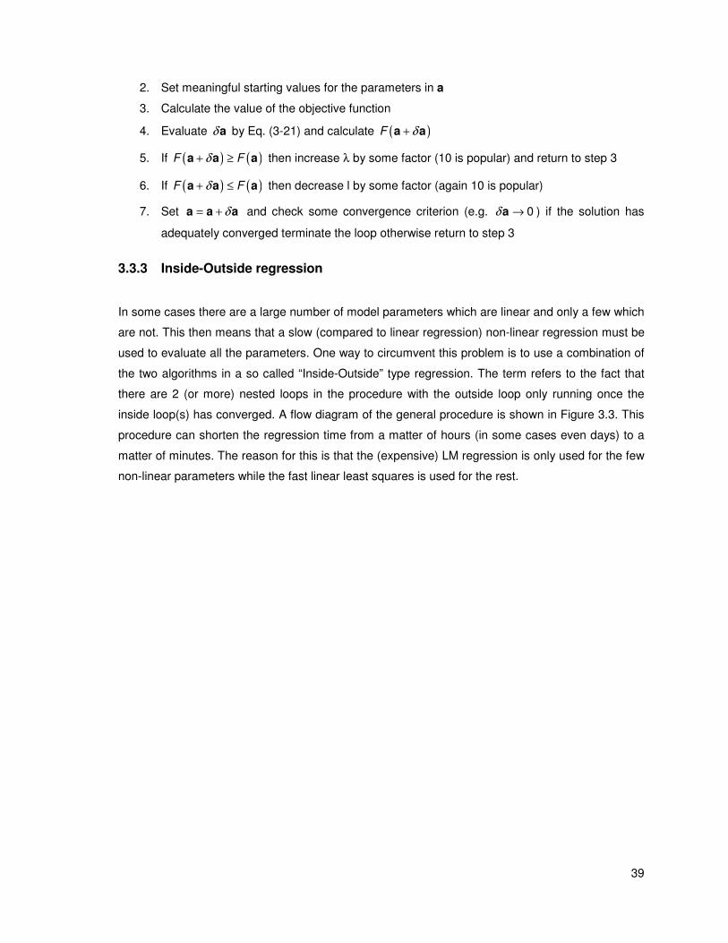
39

2. Set meaningful starting values for the parameters in a

3. Calculate the value of the objective function

4. Evaluate δ a by Eq. (3-21) and calculate ( )F δ+a a

5. If ( ) ( )F Fδ+ ≥a a a then increase λ by some factor (10 is popular) and return to step 3

6. If ( ) ( )F Fδ+ ≤a a a then decrease l by some factor (again 10 is popular)

7. Set δ= +a a a and check some convergence criterion (e.g. 0δ →a ) if the solution has

adequately converged terminate the loop otherwise return to step 3

3.3.3 Inside-Outside regression

In some cases there are a large number of model parameters which are linear and only a few which

are not. This then means that a slow (compared to linear regression) non-linear regression must be

used to evaluate all the parameters. One way to circumvent this problem is to use a combination of

the two algorithms in a so called “Inside-Outside” type regression. The term refers to the fact that

there are 2 (or more) nested loops in the procedure with the outside loop only running once the

inside loop(s) has converged. A flow diagram of the general procedure is shown in Figure 3.3. This

procedure can shorten the regression time from a matter of hours (in some cases even days) to a

matter of minutes. The reason for this is that the (expensive) LM regression is only used for the few

non-linear parameters while the fast linear least squares is used for the rest.

40

Figure 3.3 Flow diagram for the “Inside-Outside” regression technique

3.3.4 Implementation

Both the non-linear and linear least squared fits were coded in Compaq Visual Fortran (CVF), since

Fortran is well known to be able to handle computations very efficiently. CVF did not provide a

simple way to access databases so since all the other data processing was done in VBA, the

Collect the data from the DDB

via an SQL query

Guess the linear

parameters B’ – Eq. (4-2)

Guess the non-linear parameters (these

are the parameters of C(Tb) – (see Eq.

(4-3)), they are needed for the starting

point of the LM regression)

Solve for the non-linear

parameters using LM

Check if the non-linear

parameters have converged

within a certain tolerance

Solve for the linear parameters

(linear least squares)

Set the initial C(Tb) parameters

equal to the old C(Tb) ones

Store the results

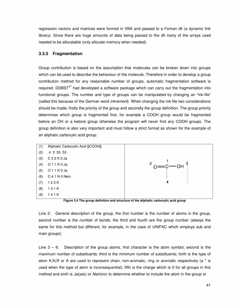
41

regression vectors and matrices were formed in VBA and passed to a Fortran dll (a dynamic link

library). Since there are huge amounts of data being passed to the dll many of the arrays used

needed to be allocatable (only allocate memory when needed).

3.3.5 Fragmentation

Group contribution is based on the assumption that molecules can be broken down into groups

which can be used to describe the behaviour of the molecule. Therefore in order to develop a group

contribution method for any reasonable number of groups, automatic fragmentation software is

required. DDBST47

had developed a software package which can carry out the fragmentation into

functional groups. The number and type of groups can be manipulated by changing an “ink-file”

(called this because of the German word inkrement). When changing the ink-file two considerations

should be made; firstly the priority of the group and secondly the group definition. The group priority

determines which group is fragmented first, for example a COOH group would be fragmented

before an OH or a ketone group otherwise the program will never find any COOH groups. The

group definition is also very important and must follow a strict format as shown for the example of

an aliphatic carboxylic acid group:

(1) Aliphatic Carboxylic Acid §COOH§

(2) 4 3 53 53

(3) C 3 2 K 0 Ja

(4) O 1 1 K 0 Ja

(5) O 1 1 K 0 Ja

(6) C 4 1 N 0 Nein

(7) 1 2 2 K

(8) 1 3 1 K

(9) 1 4 1 K

Figure 3.4 The group definition and structure of the aliphatic carboxylic acid group

Line 2: General description of the group, the first number is the number of atoms in the group,

second number is the number of bonds, the third and fourth are the group number (always the

same for this method but different, for example, in the case of UNIFAC which employs sub and

main groups)

Line 3 – 6: Description of the group atoms, first character is the atom symbol; second is the

maximum number of substituents; third is the minimum number of substituents; forth is the type of

atom K,N,R or A are used to represent chain, non-aromatic, ring or aromatic respectively (a * is

used when the type of atom is inconsequential); fifth is the charge which is 0 for all groups in this

method and sixth is Ja(yes) or Nein(no) to determine whether to include the atom in the group or

42

not (in this example the fourth atom is not included since it is not part of the group but still important

for the correct definition of the group)

Line 7 – 9: Description of the bonds in the group, the first 2 numbers are the atom numbers

between which the bond occurs; the third number is the number of bonds (i.e. single, double etc);

the last character is the type of bond (A, R or K used – same meaning as previously).

43

4 DEVELOPMENT OF THE METHOD

4.1 Model development

It is fairly intuitive that the accuracy of the regression should be increased with the number of model

parameters. However the more parameters there are the more difficult it becomes to accurately fit

the model parameters. The reason for this is that very often the parameters are intercorrelated, i.e.

they contribute to the same effect in some way. This means that there are some parameter values

that produce very good fits but are physically very unrealistic. This became very apparent when

fitting the equations in Section 2.2; consider the example of the model given by Eq. (2-27). Figure

4.1 and Figure 4.2 show the marked difference in the plots for ( )vap vapH R Z∆ ∆ , however the vapour

pressure plots look remarkably similar. Even though the vapour pressure fit in Figure 4.1 is slightly

better than that of Figure 4.2 it shows that seemingly correct parameters can be very wrong. This

problem is made much worse when fitting to only a small section of the data.

1

2

3

4

5

6

7

8

9

250 300 350 400 450 500 550 600

Temperature (K)

ln(P

/1 k

Pa

)

3.5

3.6

3.7

3.8

3.9

4.0

4.1

4.2

4.3

4.4

250 300 350 400 450 500 550 600

Temperature (K)

∆∆ ∆∆H

va

p/(

R∆∆ ∆∆

Zv

ap)

x 1

0-3

(K)

Tb

Figure 4.1 A proper fit for the Eq. (2-27)

1

2

3

4

5

6

7

8

9

250 300 350 400 450 500 550 600

Temperature (K)

ln(P

/1 k

Pa

)

3.5

3.6

3.7

3.8

3.9

4.0

4.1

4.2

4.3

4.4

250 300 350 400 450 500 550 600

Temperature (K)

∆∆ ∆∆H

va

p/(

R∆∆ ∆∆

Zv

ap

) x

10

-3 (K

)

Tb

Figure 4.2 A physically unrealistic fit for Eq. (2-27)

44

It is for this reason that the objective of this work was to develop an equation with as few

parameters as possible. From all the equations presented above the one which stands out for both

its simplicity and accuracy is the Antoine equation. At very low temperatures (in the vicinity of T=C)

the Antoine equation diverges, however since C is typically in the range of 40K to 70K this is

outside the range of practical interest (but may still cause problems, e.g. in simulation iterations).

The problem of intercorrelated parameters is still a weakness, and therefore the Antoine equation

needed to be modified. An obvious choice would be to use the normal boiling point instead of the

parameter A since there are a large number of normal boiling point data available in literature. This

is done by using the normal boiling point as a datum point, this results in the following equation:

ln b

atm b b

T TP B B B

P T C T C T C T C

−−= − = ×

− − − − (4-1)

This new model however still suffers from the fact that the model parameters B and C need to be

regressed to data (and since B and C are intercorrelated no meaningful group contribution method

can be developed). It has been observed by Thomson34

that the C parameter correlates with the

normal boiling point and the equation can be written in the following form:

ln '( )

b

atm b

T TPB

P T C T

−=

− (4-2)

While the value of C was simply assumed to be / 8bT in the model of Nannoolal et al.8, the

following function was found to give better representation of both large and small molecules as well

as providing greatly improved representation of low pressure data:

1.485

0.485( ) 2.65

135

bb

TC T K

K= − + (4-3)

The advantage of this C-parameter correlation is that it not only provides a better representation of

the data but also improves the group contribution estimation of B’. As with the model of Nannoolal

et al.8, Eq. (4-2) cannot model the aliphatic alcohols and carboxylic acids correctly and for this

reason a logarithmic correction term was added (for all other compounds D’ is set to zero):

ln ' ' ln( )

b

atm b b

T TP TB D

P T C T T

−= +

− (4-4)

45

The effect of this correction term is very significant and therefore the predictions of the aliphatic

alcohols and carboxylic acids are dramatically improved.

-2.5

-0.5

1.5

3.5

5.5

7.5

9.5

250 300 350 400 450 500 550 600

Temperature (K)

ln(P

s/1

kP

a)

Figure 4.3 ln(Ps/1 kPa) vs. T for 1-butanol (♦ - data from the DDB,

_____ with the logarithm term, - - - - without the

logarithm term)

3.5

4

4.5

5

5.5

6

6.5

7

7.5

250 300 350 400 450 500 550 600

Temperature (K)

∆∆ ∆∆H

va

p/(

R∆∆ ∆∆

Zv

ap

) x

10

-3 (K

)

Figure 4.4 ∆∆∆∆Hvap/(R∆∆∆∆Zvap) for 1-butanol (♦ - data from SRK using the MC28

alpha function and the Watson equation

(Eq. (2-36) with m = 0.473), _____

prediction with the logarithm term, - - - - prediction without the logarithm term)

46

Consider the example of 1-butanol; Figure 4.3 shows the improved vapour pressure fit (the error is

reduced from 7.5% to 2.8%). This improvement is not so visible from the vapour pressure plot but

the plot of ( )vap vapH R Z∆ ∆ quite clearly shows the substantial improvement that the logarithmic term

makes to the physical realism of the model parameters (It is interesting to note that even a direct fit

of all three Antoine parameters does not give an adequate description of the ( )vap vapH R Z∆ ∆ curve

and therefore a logarithmic correction term is also needed; in this form it is known as the modified

Antoine.). Both B’ and D’ in Eq. (4-4) are calculated from group contribution. Due to significant

intercorrelation simultaneous regression of B’ and the group increments for D’ was required.

In an attempt to make the model more widely applicable an effort was made to correlate the model

parameters with properties which can be predicted ab initio. One such property is the polarizability,

which is basically the tendency of a molecule to be polarized by an external electric field. The

polarizability data was taken from ab initio DFT calculations using the hybrid functional B3LYP and

the electron representation 663B in the program Gaussian 2003. As shown in Figure 4.5 the

correlation is very good for the n-alkanes, however when the data for the hydrocarbons is plotted

(Figure 4.6) it is clear that one can not draw any meaningful correlations from the data. There was a

fairly good correlation between the boiling point and polarizability for the hydrocarbons as shown in

Figure 4.7, however no meaningful results could be obtained as the scatter was too high.

9.2

9.4

9.6

9.8

10

10.2

10.4

0 20 40 60 80 100 120 140 160

Polarizability (C.m2.V-1)

B'

Figure 4.5 B’ vs. polarizability for the n-alkanes

47

9

9.2

9.4

9.6

9.8

10

10.2

10.4

0 20 40 60 80 100 120 140 160

Polarizability (C.m2.V -1)

B'

Figure 4.6 B’ vs. polarizability for hydrocarbons

100

150

200

250

300

350

400

450

500

550

600

20 40 60 80 100 120 140 160

Polarizability (C.m2.V -1)

Tb

(K

)

Figure 4.7 Tb vs. polarizability for hydrocarbons

Beside the advantage of having the parameters predicted with no experimental data, an approach

like this also would enable the model to be split into different part for different effects (non-polar,

polar and hydrogen bonding). The advantage of this is that the parameters then become physically

meaningful and could be used, for example, to predict the Hansen solubility parameters.

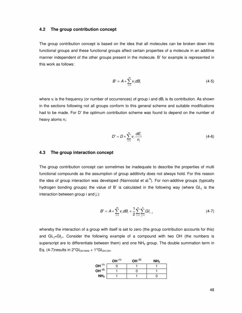
48

4.2 The group contribution concept

The group contribution concept is based on the idea that all molecules can be broken down into

functional groups and these functional groups affect certain properties of a molecule in an additive

manner independent of the other groups present in the molecule. B’ for example is represented in

this work as follows:

1

'm

i ii

B A v dB=

= +∑ (4-5)

where vi is the frequency (or number of occurrences) of group i and dBi is its contribution. As shown

in the sections following not all groups conform to this general scheme and suitable modifications

had to be made. For D’ the optimum contribution scheme was found to depend on the number of

heavy atoms ni:

1

'm

ii

i i

dED D v

n=

= +∑ (4-6)

4.3 The group interaction concept

The group contribution concept can sometimes be inadequate to describe the properties of multi

functional compounds as the assumption of group additivity does not always hold. For this reason

the idea of group interaction was developed (Nannoolal et al.6). For non-additive groups (typically

hydrogen bonding groups) the value of B’ is calculated in the following way (where GIi-j is the

interaction between group i and j.):

1 1 1

1'

2

m n n

i i i ji i j

B A v dB GI −= = =

= + +∑ ∑∑ (4-7)

whereby the interaction of a group with itself is set to zero (the group contribution accounts for this)

and GIi-j=GIj-i. Consider the following example of a compound with two OH (the numbers is

superscript are to differentiate between them) and one NH2 group. The double summation term in

Eq. (4-7)results in 2*GIOH-NH2 + 1*GIOH-OH.

OH (1)

OH (2)

NH2

OH (1)

0 1 1

OH (2)

1 0 1

NH2 1 1 0

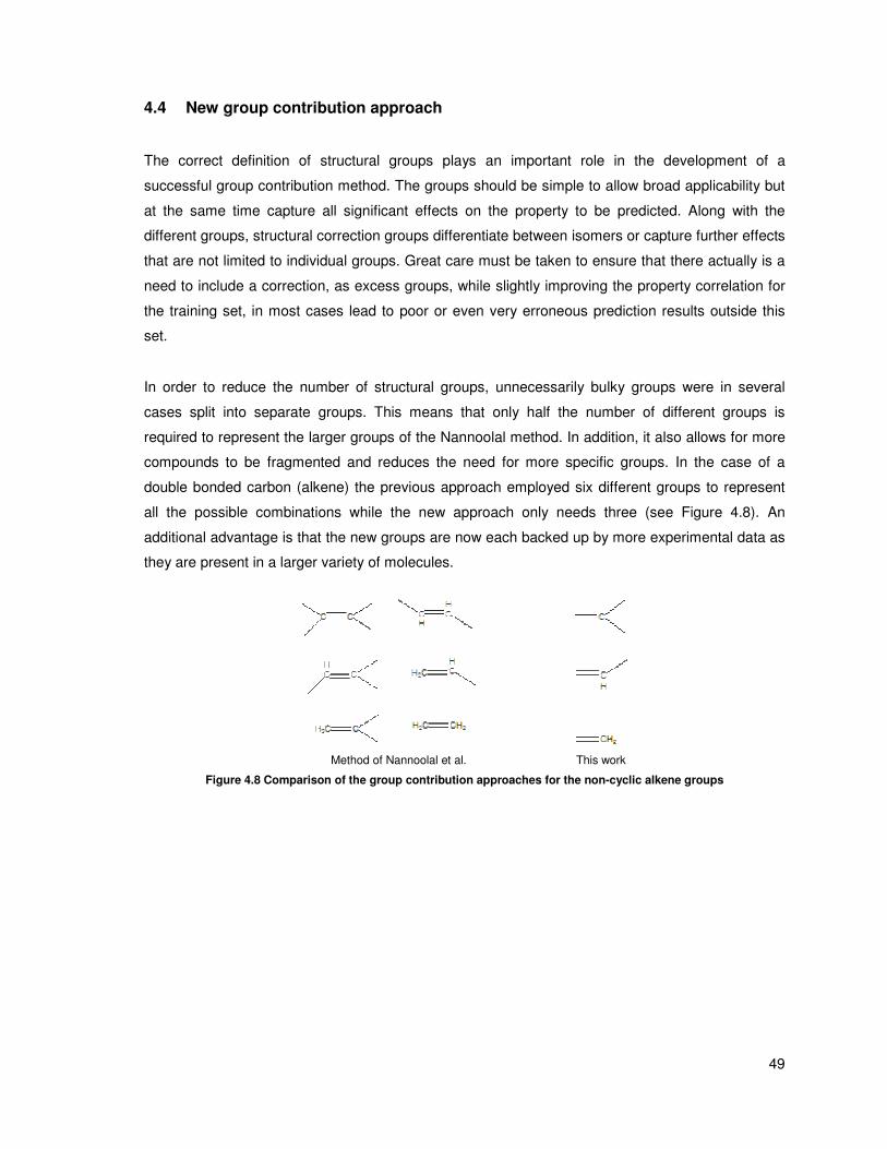
49

4.4 New group contribution approach

The correct definition of structural groups plays an important role in the development of a

successful group contribution method. The groups should be simple to allow broad applicability but

at the same time capture all significant effects on the property to be predicted. Along with the

different groups, structural correction groups differentiate between isomers or capture further effects

that are not limited to individual groups. Great care must be taken to ensure that there actually is a

need to include a correction, as excess groups, while slightly improving the property correlation for

the training set, in most cases lead to poor or even very erroneous prediction results outside this

set.

In order to reduce the number of structural groups, unnecessarily bulky groups were in several

cases split into separate groups. This means that only half the number of different groups is

required to represent the larger groups of the Nannoolal method. In addition, it also allows for more

compounds to be fragmented and reduces the need for more specific groups. In the case of a

double bonded carbon (alkene) the previous approach employed six different groups to represent

all the possible combinations while the new approach only needs three (see Figure 4.8). An

additional advantage is that the new groups are now each backed up by more experimental data as

they are present in a larger variety of molecules.

Method of Nannoolal et al.

This work

Figure 4.8 Comparison of the group contribution approaches for the non-cyclic alkene groups

50

5 RESULTS AND DISCUSSION

5.1 Hydrocarbon compounds

As mentioned earlier the new C-parameter employed in this work leads to a better representation of

data for molecules of different sizes, as illustrated in Figure 5.1 to Figure 5.4. These figures show

the performance of the vapour pressure equation (B’ was regressed to the experimental data) using

the C-parameter correlation of Nannoolal et al. compared to the new C-correlation (Eq.(4-3)). While

both models perform adequately in the case of octadecane, only the new correlation is at the same

time sufficiently suitable for propane.

Analysis of the hydrocarbon vapour pressure regressions revealed that data for some of the more

complex compounds were not very well represented by the groups that were already in use and

therefore the more specific structural groups, shown in Table 5.1, had to be added to account for

several structural effects.

Table 5.1 New hydrocarbon structural groups (Ink No – fragmentation group number, Ref No – reference number is

used to arrange like groups (e.g. halogen groups etc) since the ink no’s have no real structure)

Ink No

Description Example Ref No

131 CH connecting two rings bonded to a carbon also connecting these rings

113

136 Ring carbon attached to 3 other ring carbons and a sidechain carbon

114

137 Ring carbon attached to 4 other ring carbons

115

134 Carbon in a ring double bonded to a sidechain carbon

128

132 Aromatic carbon bonded to an aromatic carbon in a ring

205

133 2 aromatic carbon connected outside the rings

206

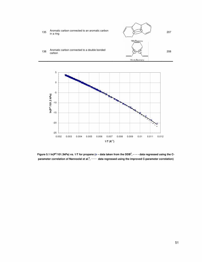
51

135 Aromatic carbon connected to an aromatic carbon in a ring

207

138 Aromatic carbon connected to a double bonded carbon

208

-25

-20

-15

-10

-5

0

5

0.002 0.003 0.004 0.005 0.006 0.007 0.008 0.009 0.01 0.011 0.012

1/T (K-1)

ln(P

s/1

01

.3 k

Pa

)

Figure 5.1 ln(Ps/101.3kPa) vs. 1/T for propane (x – data taken from the DDB

2, - - - - data regressed using the C-

parameter correlation of Nannoolal et al.8,

______ data regressed using the improved C-parameter correlation)

52

500

1 000

1 500

2 000

2 500

3 000

3 500

4 000

4 500

5 000

50 100 150 200 250 300 350 400

Temperature (K)

Pre

ss

ure

(k

Pa

)

Figure 5.2 Ps vs. T for propane (x – data taken from the DDB

2, - - - - data regressed using the C-parameter correlation

of Nannoolal et al.8,


-16

-14

-12

-10

-8

-6

-4

-2

0

0.0016 0.0018 0.002 0.0022 0.0024 0.0026 0.0028 0.003 0.0032 0.0034

1/T (K-1)

ln(P

s/1

01

.3 k

Pa

)

Figure 5.3 ln(Ps/101.3kPa) vs. 1/T for octadecane (x – data taken from the DDB

2, - - - - data regressed using the C-

parameter correlation of Nannoolal et al.8,


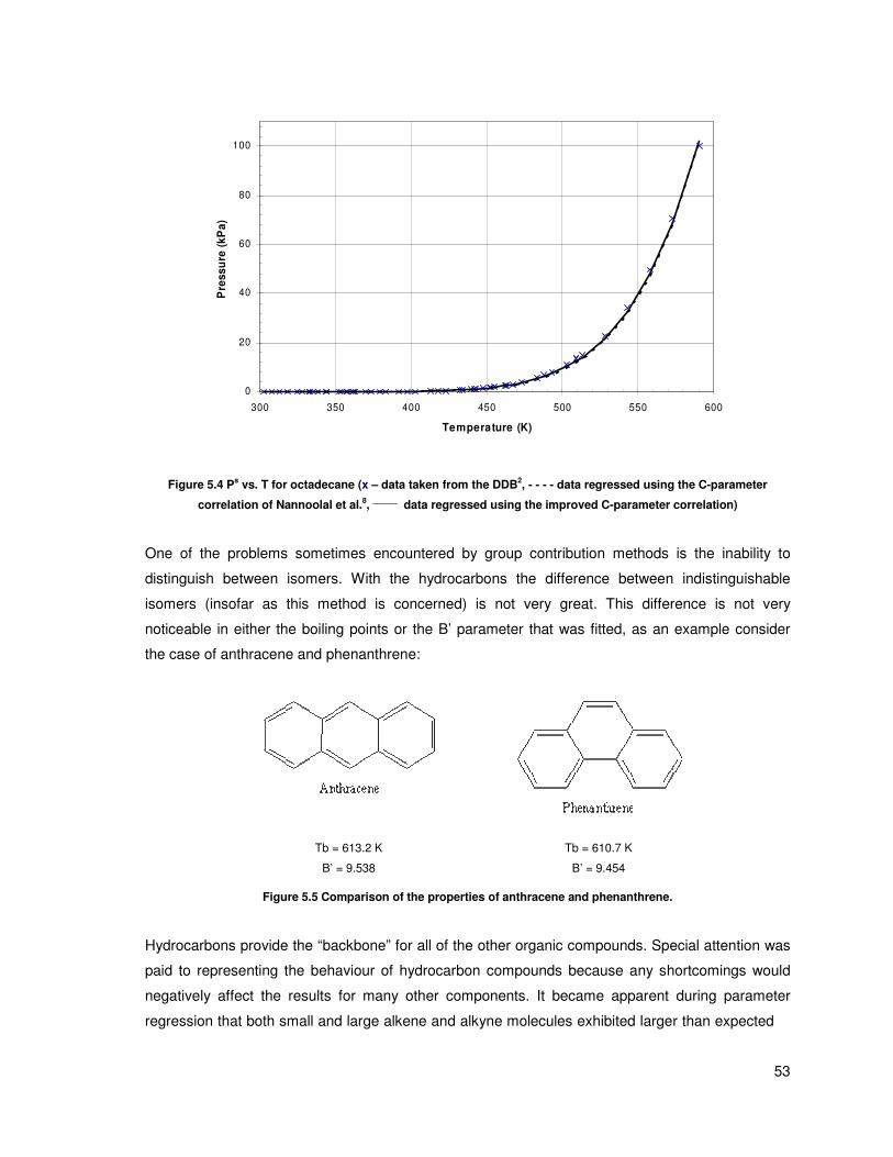
53

0

20

40

60

80

100

300 350 400 450 500 550 600

Temperature (K)

Pre

ss

ure

(k

Pa

)

Figure 5.4 Ps vs. T for octadecane (x – data taken from the DDB

2, - - - - data regressed using the C-parameter

correlation of Nannoolal et al.8,


One of the problems sometimes encountered by group contribution methods is the inability to

distinguish between isomers. With the hydrocarbons the difference between indistinguishable

isomers (insofar as this method is concerned) is not very great. This difference is not very

noticeable in either the boiling points or the B’ parameter that was fitted, as an example consider

the case of anthracene and phenanthrene:

Tb = 613.2 K

B’ = 9.538

Tb = 610.7 K

B’ = 9.454

Figure 5.5 Comparison of the properties of anthracene and phenanthrene.

Hydrocarbons provide the “backbone” for all of the other organic compounds. Special attention was

paid to representing the behaviour of hydrocarbon compounds because any shortcomings would

negatively affect the results for many other components. It became apparent during parameter

regression that both small and large alkene and alkyne molecules exhibited larger than expected

54

deviation from group contribution prediction. Further analysis revealed that the B’ values for these

components were dependant on the number of atoms present in the molecule (Figure 5.6 & Figure

5.7).

The dBi values were calculated by taking the difference between the fitted B’ values for the n-

alkenes (resp. n-alkynes) and the n-alkanes. The reason for this is that there is a large amount of

reliable data for these species; also it is important to compare like with like in order to draw any

meaningful conclusions from the data. In order to account for the size dependence a new group

(with a frequency of 1) was added to all alkene and alkyne compounds and the following size

dependant contribution scheme was used:

i i a j j ki j k

dB v dB n v dB dB= + +∑ ∑ ∑ (5-1)

The subscript i covers all normal (size independent) groups, the subscript j covers all size

dependant (e.g. alkene) groups and subscript k is for the size dependant group constants and

therefore does not have a frequency term. For example if a molecule has 3 alkene and 2 alkyne

groups there will be only be two size dependant groups, one for the alkene groups and one for the

alkyne groups (i.e. k alkyne alkenek

dB dB dB= +∑ ).

-0.4

-0.2

0

0.2

0.4

0.6

0.8

1

0 2 4 6 8 10 12 14

number of atoms

dB

i

Figure 5.6 dBi vs. number of atoms for different alkynes (♦ – dBi data for each compound, ____

a linear least squares

fit)

55

-0.4

-0.3

-0.2

-0.1

0

0.1

0.2

0 5 10 15 20

number of atoms

dB

i

Figure 5.7 dBi vs. number of atoms for different alkenes (♦ – dBi data for each compound, ____


fit)

An average percentage error of 4.1% for the vapour pressure was obtained for the hydrocarbons

which is a significant improvement compared to 5.4% obtained by Nannoolal et al.8. The mean

relative deviations for various types of hydrocarbons and both methods are given in Table 5.2 &

Table 5.3 for the different pressure regions.

Table 5.2 Relative mean deviation [%] in vapour pressure estimation for different types of hydrocarbons (this work).

The number in superscript is the number of data points used; the main number is the average percentage error of

each data point. NC – Number of compounds; ELP – Extremely low pressure P < 10 Pa; LP – Low pressure 10 Pa 500 kPa; AVE – Average error.

Group NC ELP LP MP HP AVE

Hydrocarbons 532 23.5 1102

6.8 7912

1.7 20592

5.0 4677

4.1 34294

Alkanes 149 25.1 738

8.8 3475

2.1 9023

6.4 2883

5.4 16123

Non-cyclic alkanes 101 25.8 697

9.8 2884

2.4 6873

6.7 2638

6.1 13095

Cyclic alkanes 48 13.0 41

4.0 591

1.1 2150

3.1 245

2.0 3028

Alkenes 158 19.3 45

5.2 658

1.5 3168

3.3 720

2.5 4591

Non-cyclic alkenes 120 19.3 45

5.7 514

1.5 2513

3.2 700

2.6 3772

Cyclic alkenes 30 - 3.7 108

1.6 565

4.4 20

2.0 693

Alkynes 34 - 3.7 133

1.7 666

2.5 79

2.1 878

Non-cyclic alkynes 34 - 3.7 133

1.7 666

2.5 79

2.1 878

Aromatic hydrocarbons 140 20.4 312

5.4 3197

1.5 6291

2.1 977

3.3 10784

56

Table 5.3 Relative mean deviation [%] in vapour pressure estimation for different types of hydrocarbons (Nannoolal

et al.). The number in superscript is the number of data points used; the main number is the average percentage

error of each data point. NC – Number of compounds; ELP – Extremely low pressure P < 10 Pa; LP – Low pressure

10 Pa 500 kPa; AVE – Average

error.



9.0 7744

1.7 20255

4.2 4455

5.4 33567

Alkanes 149 62.6 738

12.1 3475

1.8 9023

4.7 2883

7.3 16123

Non-cyclic alkanes 101 63.2 697

13.5 2884

2.0 6873

5.0 2638

8.4 13095

Cyclic alkanes 48 51.4 41

5.5 591

0.9 2150

2.3 245

2.6 3028

Alkenes 154 50.3 45

6.4 490

1.5 2872

3.0 540

2.9 3947

Non-cyclic alkenes 116 50.3 45

7.4 346

1.5 2217

3.0 520

3.1 3128

Cyclic alkenes 30 - 4.3 108

1.8 565

2.2 20

2.2 693

Alkynes 33 - 4.9 133

2.0 625

9.6 37

2.8 795

Non-cyclic alkynes 33 - 4.9 133

2.0 625

9.6 37

2.8 795

Aromatic hydrocarbons 140 25.8 312

6.5 3197

1.7 6291

3.0 977

3.9 10784

The greatest improvement was found for the aliphatic hydrocarbons, where the error at ELP

(extremely low pressure < 10 Pa) is significantly improved from the method of Nannoolal et al.8. The

errors at high pressures are slightly worse than the previous method, this is to be expected because

as shown in paragraph 2.2.1.1 the Antoine equation is deficient at high pressures and therefore

there must be a trade-off between the high and the low pressure errors. This slight decrease in the

error is compensated for with the large improvement of the low pressure errors.

5.2 Oxygen compounds

Oxygen compounds exhibited the largest deviation in case of both the component specific and

group specific regressions. The largest deviations were observed for aliphatic alcohols and

carboxylic acids. For this reason a logarithmic correction term (Eq.(4-4)) was added to properly

model the data. Figure 5.8 & Figure 5.9 show the difference between results with and without this

modification in case of 1-nonanol. A similar kind of deviation was observed for carboxylic acids and

is shown for palmitic acid in Figure 5.10 & Figure 5.11. As mentioned above (see paragraph 4.1)

this logarithmic correction term not only provides a better representation of the vapour pressure

curve but also makes the model more physically realistic.

57

-14

-12

-10

-8

-6

-4

-2

0

2

4

0.0014 0.0019 0.0024 0.0029 0.0034

1/T (K-1)

ln(P

s/1

01

.3 k

Pa

)

Figure 5.8 ln(Ps/101.3kPa) vs. 1/T for 1-nonanol (x – data taken from the DDB

2, - - - - data regressed using the method

of Nannoolal et al.8,

______ data regressed using the new logarithmic correction)

500

1 000

1 500

2 000

2 500

3 000

3 500

4 000

4 500

5 000

250 300 350 400 450 500 550 600 650 700

Temperature (K)

Pre

ss

ure

(k

Pa

)

Figure 5.9 Ps vs. T for 1-nonanol (x – data taken from the DDB

2, - - - - data regressed using the method of Nannoolal

et al.8,


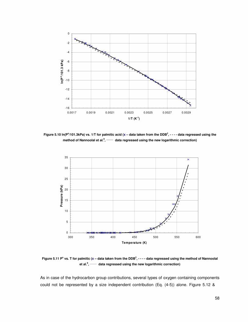
58

-16

-14

-12

-10

-8

-6

-4

-2

0

0.0017 0.0019 0.0021 0.0023 0.0025 0.0027 0.0029

1/T (K-1)

ln(P

s/1

01

.3 k

Pa

)

Figure 5.10 ln(Ps/101.3kPa) vs. 1/T for palmitic acid (x – data taken from the DDB

2, - - - - data regressed using the

method of Nannoolal et al.8,


0

5

10

15

20

25

30

35

300 350 400 450 500 550 600

Temperature (K)

Pre

ss

ure

(k

Pa

)

Figure 5.11 Ps vs. T for palmitic (x – data taken from the DDB

2, - - - - data regressed using the method of Nannoolal

et al.8,


As in case of the hydrocarbon group contributions, several types of oxygen containing components

could not be represented by a size independent contribution (Eq. (4-5)) alone. Figure 5.12 &

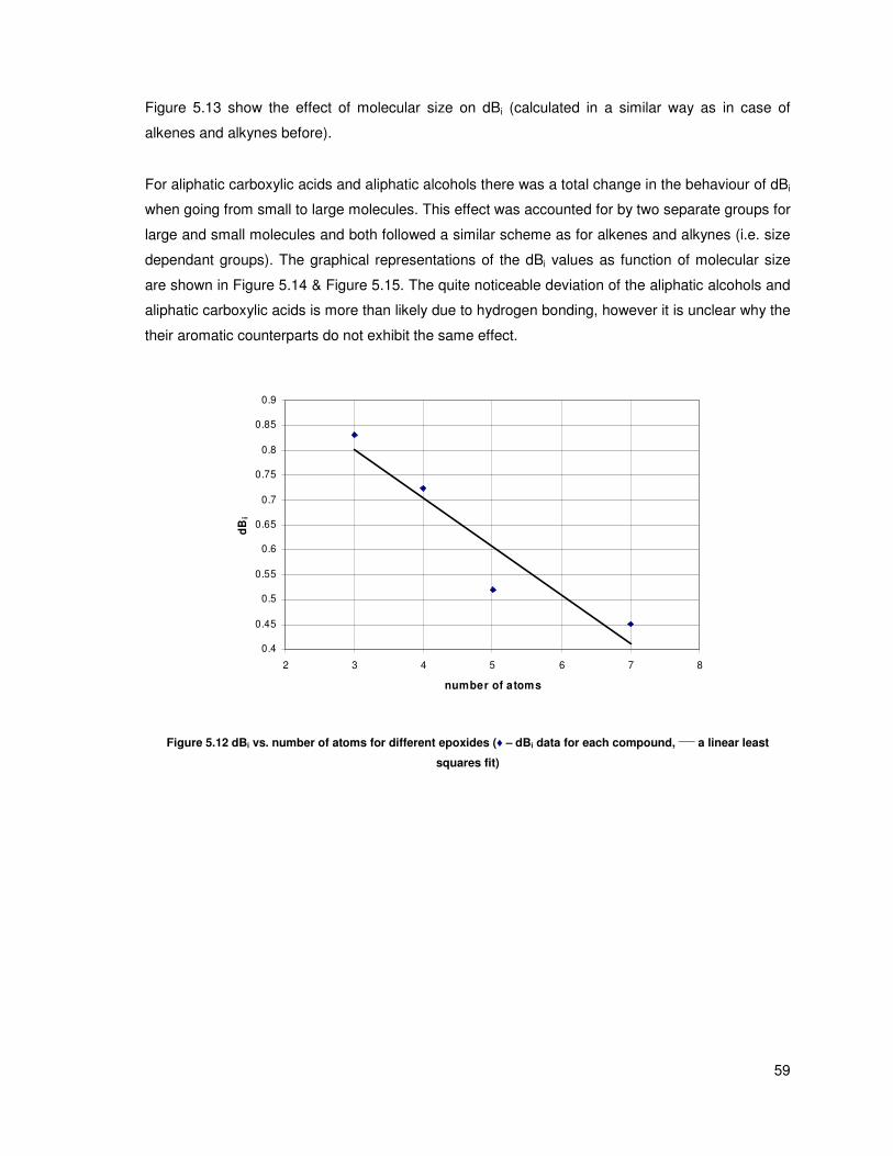
59

Figure 5.13 show the effect of molecular size on dBi (calculated in a similar way as in case of

alkenes and alkynes before).

For aliphatic carboxylic acids and aliphatic alcohols there was a total change in the behaviour of dBi

when going from small to large molecules. This effect was accounted for by two separate groups for

large and small molecules and both followed a similar scheme as for alkenes and alkynes (i.e. size

dependant groups). The graphical representations of the dBi values as function of molecular size

are shown in Figure 5.14 & Figure 5.15. The quite noticeable deviation of the aliphatic alcohols and

aliphatic carboxylic acids is more than likely due to hydrogen bonding, however it is unclear why the

their aromatic counterparts do not exhibit the same effect.

0.4

0.45

0.5

0.55

0.6

0.65

0.7

0.75

0.8

0.85

0.9

2 3 4 5 6 7 8

number of atoms

dB

i

Figure 5.12 dBi vs. number of atoms for different epoxides (♦ – dBi data for each compound, ____

a linear least

squares fit)

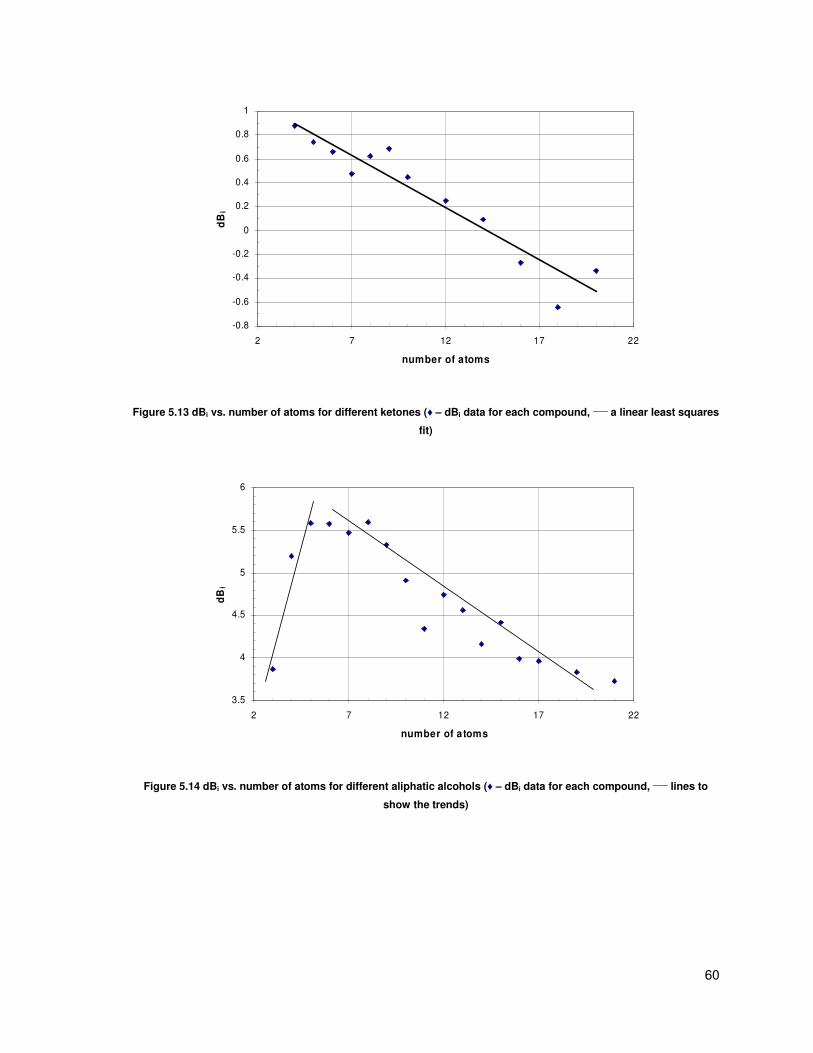
60

-0.8

-0.6

-0.4

-0.2

0

0.2

0.4

0.6

0.8

1

2 7 12 17 22

number of atoms

dB

i

Figure 5.13 dBi vs. number of atoms for different ketones (♦ – dBi data for each compound, ____


fit)

3.5

4

4.5

5

5.5

6

2 7 12 17 22

number of atoms

dB

i

Figure 5.14 dBi vs. number of atoms for different aliphatic alcohols (♦ – dBi data for each compound, ____

lines to

show the trends)

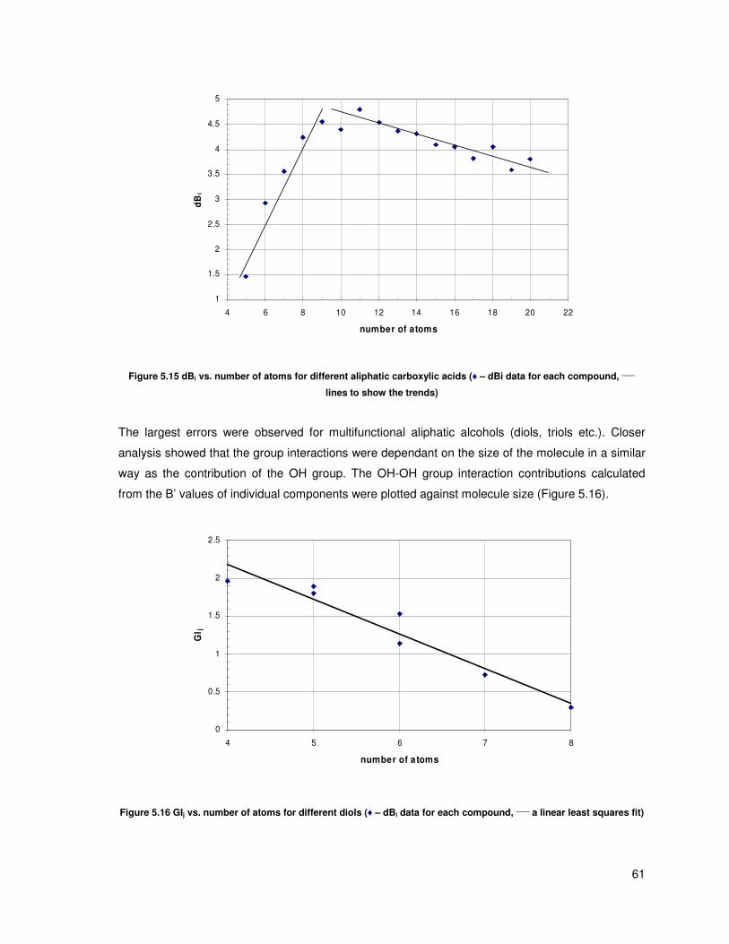
61

1

1.5

2

2.5

3

3.5

4

4.5

5

4 6 8 10 12 14 16 18 20 22

number of atoms

dB

i

Figure 5.15 dBi vs. number of atoms for different aliphatic carboxylic acids (♦ – dBi data for each compound, ____

lines to show the trends)

The largest errors were observed for multifunctional aliphatic alcohols (diols, triols etc.). Closer

analysis showed that the group interactions were dependant on the size of the molecule in a similar

way as the contribution of the OH group. The OH-OH group interaction contributions calculated

from the B’ values of individual components were plotted against molecule size (Figure 5.16).

0

0.5

1

1.5

2

2.5

4 5 6 7 8

number of atoms

GI j

Figure 5.16 GIj vs. number of atoms for different diols (♦ – dBi data for each compound, ____

a linear least squares fit)

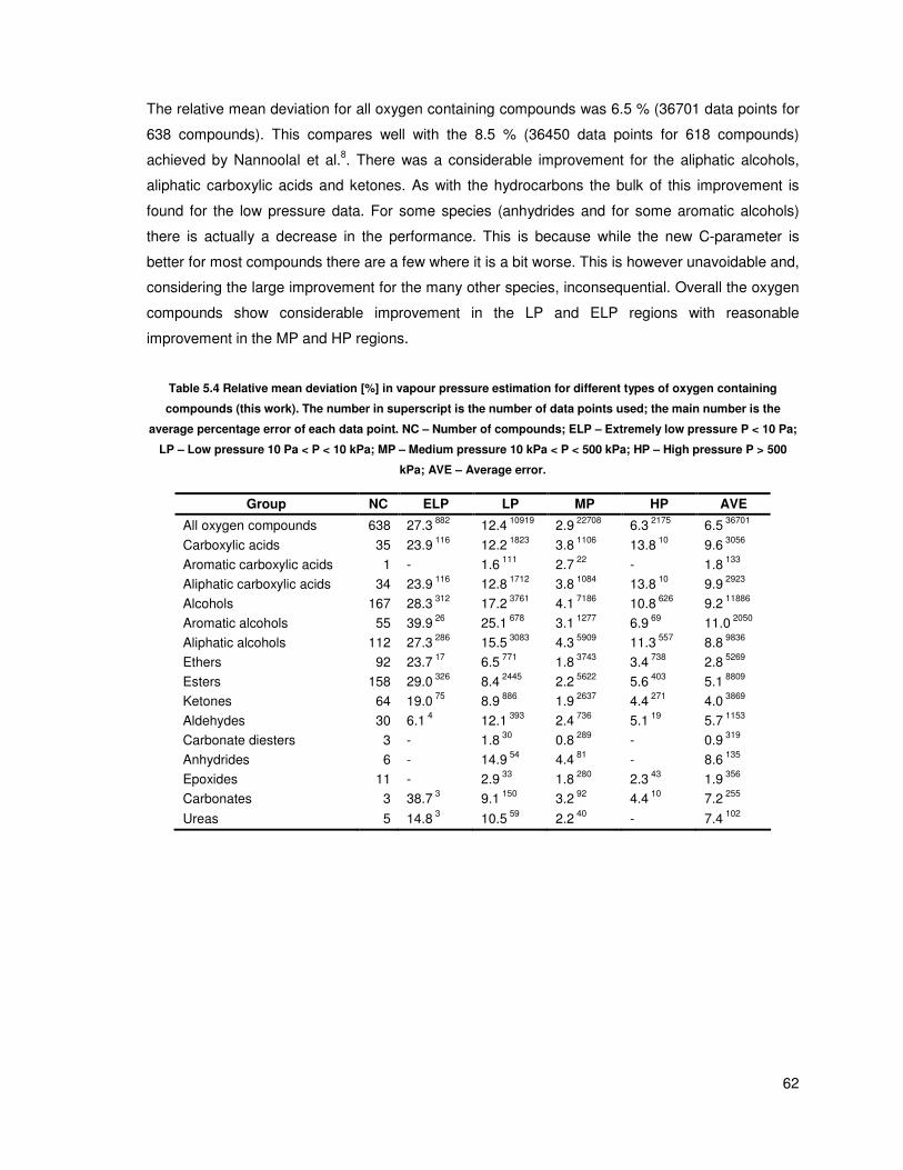
62

The relative mean deviation for all oxygen containing compounds was 6.5 % (36701 data points for

638 compounds). This compares well with the 8.5 % (36450 data points for 618 compounds)

achieved by Nannoolal et al.8. There was a considerable improvement for the aliphatic alcohols,

aliphatic carboxylic acids and ketones. As with the hydrocarbons the bulk of this improvement is

found for the low pressure data. For some species (anhydrides and for some aromatic alcohols)

there is actually a decrease in the performance. This is because while the new C-parameter is

better for most compounds there are a few where it is a bit worse. This is however unavoidable and,

considering the large improvement for the many other species, inconsequential. Overall the oxygen

compounds show considerable improvement in the LP and ELP regions with reasonable

improvement in the MP and HP regions.

Table 5.4 Relative mean deviation [%] in vapour pressure estimation for different types of oxygen containing

compounds (this work). The number in superscript is the number of data points used; the main number is the

average percentage error of each data point. NC – Number of compounds; ELP – Extremely low pressure P < 10 Pa;

LP – Low pressure 10 Pa 500

kPa; AVE – Average error.


All oxygen compounds 638 27.3 882

12.4 10919

2.9 22708

6.3 2175

6.5 36701

Carboxylic acids 35 23.9 116

12.2 1823

3.8 1106

13.8 10

9.6 3056

Aromatic carboxylic acids 1 - 1.6 111

2.7 22

- 1.8 133

Aliphatic carboxylic acids 34 23.9 116

12.8 1712

3.8 1084

13.8 10

9.9 2923

Alcohols 167 28.3 312

17.2 3761

4.1 7186

10.8 626

9.2 11886

Aromatic alcohols 55 39.9 26

25.1 678

3.1 1277

6.9 69

11.0 2050

Aliphatic alcohols 112 27.3 286

15.5 3083

4.3 5909

11.3 557

8.8 9836

Ethers 92 23.7 17

6.5 771

1.8 3743

3.4 738

2.8 5269

Esters 158 29.0 326

8.4 2445

2.2 5622

5.6 403

5.1 8809

Ketones 64 19.0 75

8.9 886

1.9 2637

4.4 271

4.0 3869

Aldehydes 30 6.1 4

12.1 393

2.4 736

5.1 19

5.7 1153

Carbonate diesters 3 - 1.8 30

0.8 289

- 0.9 319

Anhydrides 6 - 14.9 54

4.4 81

- 8.6 135

Epoxides 11 - 2.9 33

1.8 280

2.3 43

1.9 356

Carbonates 3 38.7 3

9.1 150

3.2 92

4.4 10

7.2 255

Ureas 5 14.8 3

10.5 59

2.2 40

- 7.4 102

63

Table 5.5 Relative mean deviation [%] in vapour pressure estimation for different types of oxygen containing

compounds (Nannoolal et al.8). The number in superscript is the number of data points used; the main number is

the average percentage error of each data point. NC – Number of compounds; ELP – Extremely low pressure P < 10

Pa; LP – Low pressure 10 Pa 500



All oxygen compounds 618 60.1 882

15.4 10810

3.2 22544

7.9 2151

8.5 36404

Carboxylic acids 34 106.8 116

17.2 1819

3.5 1100

10.6 10

15.7 3046

Aromatic carboxylic acids 1 - 13.7 111

2.4 22

- 11.8 133

Aliphatic carboxylic acids 33 106.8 116

17.5 1708

3.6 1078

10.6 10

15.8 2913

Alcohols 162 80.8 312

21.7 3732

4.7 7119

13.0 602

12.5 11766

Aromatic alcohols 55 33.5 26

24.5 678

3.3 1277

6.3 69

10.8 2050

Aliphatic alcohols 107 85.1 286

21.0 3054

5.0 5842

13.9 533

12.9 9716

Ethers 91 28.3 17

7.6 768

2.1 3738

4.7 738

3.3 5261

Esters 154 30.8 326

9.0 2432

2.3 5602

7.0 403

5.5 8776

Ketones 63 47.2 75

11.8 886

2.0 2637

5.6 271

5.3 3869

Aldehydes 29 20.9 4

15.0 392

2.3 731

5.1 19

6.8 1147

Carbonate diesters 3 - 4.5 30

0.8 289

- 1.1 319

Anhydrides 6 - 8.5 54

3.9 81

- 5.7 135

Epoxides 11 - 4.6 33

2.2 280

2.4 43

2.4 356

Carbonates 3 27.8 3

10.8 150

6.3 92

14.0 10

9.5 255

Ureas 4 104.2 3

14.9 39

1.4 38

- 11.8 80

5.3 Nitrogen compounds

Most nitrogen compounds did not show significant deviation from the model predictions. Only in the

case of primary aliphatic amines, nitriles and aliphatic isocyanates similar extensions as in the case

of some of the oxygenated compounds were required. Figure 5.17 to Figure 5.19 show the dBi

contributions for these compound classes as function of molecular size.

Differentiation had to be made between aliphatic and aromatic isocyanates. Groups were also

added for cyclic tertiary amines and the hydrazine group (in accordance with the new group

contribution approach mentioned in paragraph 4.4)

64

-0.4

-0.2

0

0.2

0.4

0.6

0.8

1

1.2

1.4

2 4 6 8 10 12 14 16 18 20

number of atoms

dB

i

Figure 5.17 dBi vs. number of atoms for different primary aliphatic amines (♦ – dBi data for each compound, ____

a

linear least squares fit)

0

0.1

0.2

0.3

0.4

0.5

0.6

2 7 12 17 22

number of atoms

dB

i

Figure 5.18 dBi vs. number of atoms for different nitriles (♦ – dBi data for each compound, ____

lines to show the

trends)

65

0.5

0.7

0.9

1.1

1.3

1.5

1.7

1.9

2.1

2.3

4 5 6 7 8 9 10

number of atoms

dB

i

Figure 5.19 dBi vs. number of atoms for different aliphatic isocyanates (♦ – dBi data for each compound, ____

a linear

least squares fit)

The relative mean deviation for all nitrogen containing compounds was 5.3% (10410 data points for

260 compounds) compared to 6.5% (10318 data points for 252 compounds) for the method of

Nannoolal et al.8. It is fairly interesting to note that even with the special attention that was paid to

the nitrile compounds there is actually a decrease in the performance of the model. As before the

reason for this is that the C-parameter causes the nitriles to deviate quite significantly from group

contribution. Even the two sets of size dependant groups could not properly account for this effect

and therefore nitrile predictions should be used with a fair bit of caution when using temperatures

far removed from the boiling point. The nitrogen compounds show a good improvement for all four

pressure ranges with some compounds exhibiting considerable improvement (e.g. the nitrates)

66

Table 5.6 Relative mean deviation [%] in vapour pressure estimation for different types of nitrogen containing






All nitrogen compounds 260 28.4 80

9.8 3521

2.5 6311

5.0 492

5.3 10410

Amides 18 12.8 1

11.6 635

3.5 549

8.3 2

7.8 1190

Isocyanates 6 4.5 2

12.3 53

4.6 63

5.8 5

7.9 123

Oximes 7 9.6 5

5.5 57

1.9 49

- 4.1 111

Nitro groups 18 31.6 21

7.7 335

3.0 412

2.7 12

5.8 780

Nitrites 2 - - 0.6 30

- 0.6 30

Azoles 1 - - 0.6 18

- 0.6 18

Nitrates 6 79.9 3

16.4 44

3.3 23

- 14.8 70

Amines 113 19.9 9

12.1 1169

2.6 2611

6.3 298

5.6 4088

Primary amines 48 21.7 3

13.7 566

2.9 1188

5.9 121

6.4 1878

Secondary amines 33 17.9 1

12.8 286

2.8 842

6.3 121

5.4 1251

Tertiary amines 25 19.2 5

8.3 295

1.8 470

6.0 29

4.5 799

Azenes 3 - 9.7 22

1.2 26

- 5.1 48

Aromatic nitrogens 41 18.7 13

7.2 657

1.8 1539

3.2 82

3.5 2291

Nitriles 35 31.5 28

6.9 483

2.3 893

2.9 98

4.4 1503

Hydrazines 7 - 6.0 63

2.9 72

- 4.3 135

Table 5.7 Relative mean deviation [%] in vapour pressure estimation for different types of nitrogen containing






All nitrogen compounds 252 61.8 80

11.6 3484

2.8 6256

7.7 492

6.5 10318

Amides 16 42.3 1

11.7 631

3.4 533

3.9 2

7.9 1170

Isocyanates 5 92.9 2

22.7 50

6.0 60

13.1 5

14.9 117

Oximes 7 8.1 5

4.3 57

2.5 49

- 3.7 111

Nitro groups 17 162.8 21

10.3 332

2.7 409

2.1 12

10.3 774

Nitrites 2 - - 6.3 30

- 6.3 30

Azoles 1 - - 0.6 18

- 0.6 18

Nitrates 6 152.9 3

31.4 44

5.9 23

- 28.2 70

Amines 112 41.3 9

14.5 1168

3.0 2606

9.0 298

6.8 4082

Primary amines 48 28.7 3

13.4 566

3.3 1188

10.8 121

6.9 1878

Secondary amines 33 83.5 1

17.3 286

2.5 842

5.5 121

6.2 1251

Tertiary amines 25 40.3 5

13.8 295

3.1 470

5.8 29

7.4 799

Azenes 0 - - - - -

Aromatic nitrogens 41 5.2 13

8.2 657

2.0 1539

4.0 82

3.8 2291

Nitriles 35 19.5 28

5.2 483

1.9 893

7.4 98

3.7 1503

Hydrazines 7 - 45.4 63

11.5 72

- 27.3 135

67

5.4 Sulfur compounds

Sulfur containing compounds showed no significant deviation in both single compound and group

contribution regressions. The average error for all sulfur containing compounds was 3.5% (3386

data points for 104 compounds) compared to 11.1% (3378 data points for 103 compounds)

obtained with the method of Nannoolal et al.8. This huge improvement in the overall error is

misleading since the massive error for the sulfoxides significantly offsets this error. When the

sulfoxides are removed from the error calculation, the error is slightly over 4% which is comparable

to the current method. This shows that the sulfur compounds follow the principle of group

contribution very well (a very good example of this is the mercaptans – sometimes known as thiols

– where the overall percentage error for 37 different compounds is only 2.2% for both methods)

Table 5.8 Relative mean deviation [%] in vapour pressure estimation for different types of sulfur containing






All sulfur compounds 104 22.6 32

7.5 769

1.7 2425

7.5 160

3.5 3386

Disulfides 8 - 1.1 74

1.3 205

2.2 8

1.2 287

Mercaptans 38 6.6 1

4.5 108

1.3 797

8.9 68

2.2 974

Thioether 50 23.9 25

9.9 317

1.6 1273

5.6 77

3.7 1692

Sulfones 1 19.9 6

17.5 59

4.9 26

21.7 7

14.6 98

Sulfon amides 3 - 11.4 18

0.1 1

- 10.8 19

Sulfoxides 1 - 4.2 141

4.9 120

- 4.5 261

Isothiocyanates 3 - 4.4 52

5.7 3

- 4.5 55

Table 5.9 Relative mean deviation [%] in vapour pressure estimation for different types of sulfur containing






All sulfur compounds 103 29.2 32

37.9 769

2.6 2421

7.2 156

11.1 3378

Disulfides 8 - 2.5 74

1.4 205

2.6 8

1.7 287

Mercaptans 37 8.3 1

3.4 108

1.4 793

9.8 64

2.2 966

Thioether 50 28.7 25

11.9 317

1.6 1273

5.5 77

4.1 1692

Sulfones 1 34.6 6

16.9 59

2.8 26

7.1 7

13.5 98

Sulfon amides 3 - 9.4 18

0.1 1

- 8.9 19

Sulfoxides 1 - 166.3 141

23.1 120

- 100.4 261

Isothiocyanates 3 - 4.5 52

5.2 3

- 4.6 55

68

5.5 Halogen compounds

Halogen compounds are unique in that there are many multifunctional compounds which in this

case were not treated like the other multifunctional species. Instead of a group interaction term

there are groups which account for compounds with 1, 2 or 3 halogen atoms attached to the same

carbon and in that way do provide some sort of group interaction. No specific problems were

observed with modelling and predicting the vapour pressure curves of these components.

For fluoro, chloro and bromo compounds sufficient data were available to regress all the group

contributions. Only in the case of iodo compounds was a single group was used due to the lack of

data. Therefore results for compounds containing iodine should be used with caution. The relative

mean deviation for all halogen containing compounds is 3.3% (19465 data points for 317

compounds) which is similar to the 4.1% obtained by the method of Nannoolal et al.8 (19344 data

points for 300 compounds). The greatest improvement is found for ELP’s where the error for the

current work is half the error obtained by the method of Nannoolal et al.8. This is due to the addition

of a couple more halogen groups (see groups 42 and 117 in Table A.1 for examples) and the new

C-parameter.

Table 5.10 Relative mean deviation [%] in vapour pressure estimation for different types of halogen containing






All halogen compounds 317 37.5 59

7.0 2329

1.8 11049

4.2 6026

3.3 19465

Fluorine compounds 86 - 8.7 481

1.9 3836

5.0 3805

3.8 8123

Chlorine compounds 108 16.6 17

6.5 973

1.6 4170

4.4 608

2.8 5768

Bromine compounds 42 47.1 40

6.2 449

1.7 781

0.4 15

4.7 1285

Iodine compounds 10 21.4 2

11.4 128

2.0 253

4.2 5

5.3 388

Table 5.11 Relative mean deviation [%] in vapour pressure estimation for different types of halogen containing






All halogen compounds 300 76.9 59

8.2 2266

2.0 10981

5.5 6026

4.1 19334

Fluorine compounds 84 - 8.3 481

2.2 3824

6.4 3805

4.5 8111

Chlorine compounds 98 39.6 17

8.1 939

2.1 4136

6.2 608

3.6 5700

Bromine compounds 42 95.7 40

9.2 449

1.9 781

2.2 15

7.4 1285

Iodine compounds 10 19.1 2

9.4 128

1.9 253

3.8 5

4.5 388

69

5.6 Other compounds

This category of species is very broad and has the highest potential for large errors due to the fact

that only few data were available for each group. This is especially true for the organometallics

where there was very limited data available and therefore predicted results should only be used as

a rough guide. Some attention was paid to the silicon containing compounds and the silicon groups

were expanded in a similar fashion to the carbon compounds. There are however much fewer

silicon groups as there are no cyclic silicon chains and much less data were available to back up

very differentiated groups. Four groups for halogen-substituted silicon were added. The relative

mean deviations are given in the following tables:

Table 5.12 Relative mean deviation [%] in vapour pressure estimation for various other compounds. The number in

superscript is the number of data points used; the main number is the average percentage error of each data point.

NC – Number of compounds; ELP – Extremely low pressure P < 10 Pa; LP – Low pressure 10 Pa 500 kPa; AVE – Average error.


Phosphorous compounds 9 10.1 7

10.7 45

4.6 49

- 7.7 101

Metals 18 - 6.0 109

2.7 278

1.2 14

3.6 401

Other compounds 13 - 7.5 150

4.4 190

- 5.8 340

Silicon compounds 68 - 9.7 383

2.5 746

2.8 138

4.7 1267

Table 5.13 Relative mean deviation [%] in vapour pressure estimation for various other compounds (Nannoolal et

al.8). The number in superscript is the number of data points used; the main number is the average percentage error

of each data point. NC – Number of compounds; ELP – Extremely low pressure P < 10 Pa; LP – Low pressure 10 Pa

 500 kPa; AVE – Average error.


Phosphorous Compounds 8 15.8 7

11.1 45

2.4 49

- 7.2 101

Metals 18 - 7.6 109

2.2 278

2.0 14

3.7 401

Other Compounds 12 - 11.2 146

5.5 188

- 8.0 334

Silicon Compounds 68 - 14.9 383

2.7 746

1.9 138

6.3 1267

5.7 Testing the method

In the preceding paragraphs (5.1-5.6) the percentage errors were shown for all data that was

contained in the model training set. Therefore in order to be sure that the model is not simply well

fitted to the training set an external test set of data was used to test the validity of the model. The

test-set contained a wide range of data so as to provide a realistic measure of the model

performance. The overall percentage error for the test set was 7.1 % for 2879 data points (160

compounds), this error is somewhat inflated because there was quite a large scatter present in the

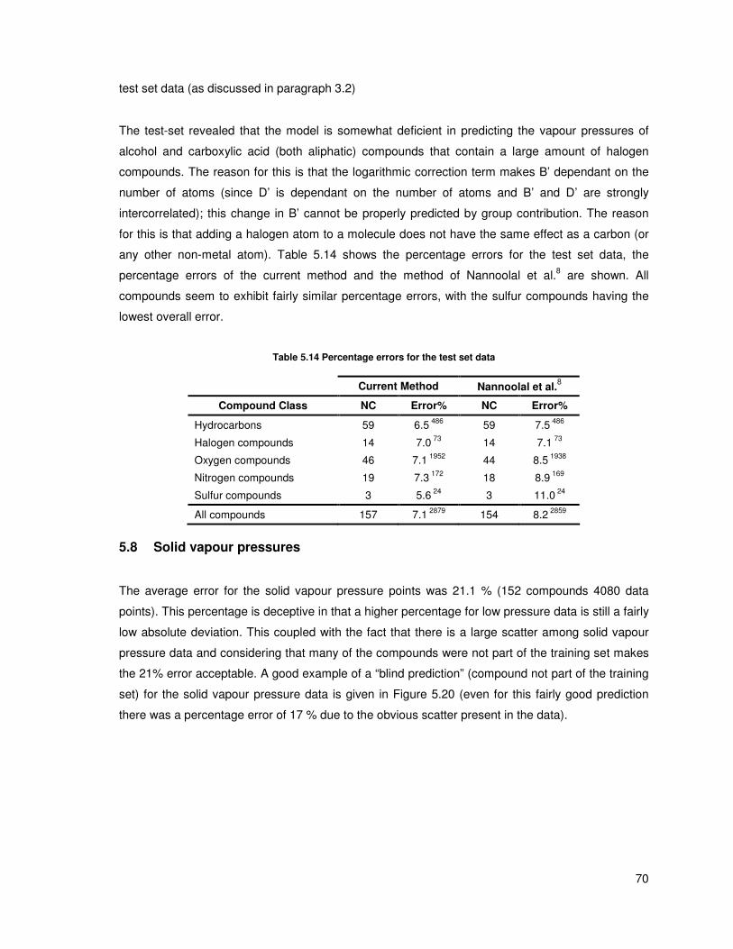
70

test set data (as discussed in paragraph 3.2)

The test-set revealed that the model is somewhat deficient in predicting the vapour pressures of

alcohol and carboxylic acid (both aliphatic) compounds that contain a large amount of halogen

compounds. The reason for this is that the logarithmic correction term makes B’ dependant on the

number of atoms (since D’ is dependant on the number of atoms and B’ and D’ are strongly

intercorrelated); this change in B’ cannot be properly predicted by group contribution. The reason

for this is that adding a halogen atom to a molecule does not have the same effect as a carbon (or

any other non-metal atom). Table 5.14 shows the percentage errors for the test set data, the

percentage errors of the current method and the method of Nannoolal et al.8 are shown. All

compounds seem to exhibit fairly similar percentage errors, with the sulfur compounds having the

lowest overall error.

Table 5.14 Percentage errors for the test set data

Current Method Nannoolal et al.8

Compound Class NC Error% NC Error%


59 7.5 486

Halogen compounds 14 7.0 73

14 7.1 73

Oxygen compounds 46 7.1 1952

44 8.5 1938

Nitrogen compounds 19 7.3 172

18 8.9 169

Sulfur compounds 3 5.6 24

3 11.0 24

All compounds 157 7.1 2879

154 8.2 2859

5.8 Solid vapour pressures

The average error for the solid vapour pressure points was 21.1 % (152 compounds 4080 data

points). This percentage is deceptive in that a higher percentage for low pressure data is still a fairly

low absolute deviation. This coupled with the fact that there is a large scatter among solid vapour

pressure data and considering that many of the compounds were not part of the training set makes

the 21% error acceptable. A good example of a “blind prediction” (compound not part of the training

set) for the solid vapour pressure data is given in Figure 5.20 (even for this fairly good prediction

there was a percentage error of 17 % due to the obvious scatter present in the data).

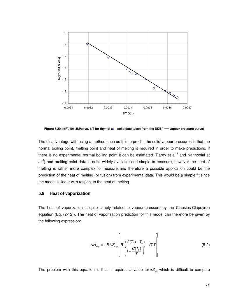
71

-14

-13

-12

-11

-10

-9

-8

0.0031 0.0032 0.0033 0.0034 0.0035 0.0036 0.0037

1/T (K-1)

ln(P

s/1

01

.3 k

Pa

)

Figure 5.20 ln(Ps/101.3kPa) vs. 1/T for thymol (x – solid data taken from the DDB

2,

____ vapour pressure curve)

The disadvantage with using a method such as this to predict the solid vapour pressures is that the

normal boiling point, melting point and heat of melting is required in order to make predictions. If

there is no experimental normal boiling point it can be estimated (Rarey et al.5 and Nannoolal et

al.6) and melting point data is quite widely available and simple to measure, however the heat of

melting is rather more complex to measure and therefore a possible application could be the

prediction of the heat of melting (or fusion) from experimental data. This would be a simple fit since

the model is linear with respect to the heat of melting.

5.9 Heat of vaporization

The heat of vaporization is quite simply related to vapour pressure by the Clausius-Clapeyron

equation (Eq. (2-12)). The heat of vaporization prediction for this model can therefore be given by

the following expression:

( )

2

( )' '

( )1

b b

vap vap

b

C T TH R Z B D T

C T

T

− ∆ = − ∆ − −

(5-2)

The problem with this equation is that it requires a value for vapZ∆ which is difficult to compute

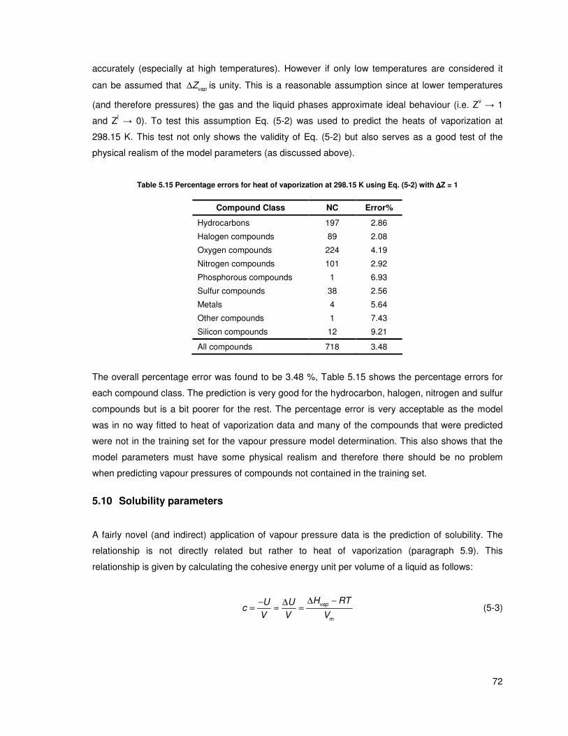
72

accurately (especially at high temperatures). However if only low temperatures are considered it

can be assumed that vapZ∆ is unity. This is a reasonable assumption since at lower temperatures

(and therefore pressures) the gas and the liquid phases approximate ideal behaviour (i.e. Zv → 1

and Zl → 0). To test this assumption Eq. (5-2) was used to predict the heats of vaporization at

298.15 K. This test not only shows the validity of Eq. (5-2) but also serves as a good test of the

physical realism of the model parameters (as discussed above).

Table 5.15 Percentage errors for heat of vaporization at 298.15 K using Eq. (5-2) with ∆∆∆∆Z = 1

Compound Class NC Error%

Hydrocarbons 197 2.86

Halogen compounds 89 2.08

Oxygen compounds 224 4.19

Nitrogen compounds 101 2.92

Phosphorous compounds 1 6.93

Sulfur compounds 38 2.56

Metals 4 5.64

Other compounds 1 7.43

Silicon compounds 12 9.21

All compounds 718 3.48

The overall percentage error was found to be 3.48 %, Table 5.15 shows the percentage errors for

each compound class. The prediction is very good for the hydrocarbon, halogen, nitrogen and sulfur

compounds but is a bit poorer for the rest. The percentage error is very acceptable as the model

was in no way fitted to heat of vaporization data and many of the compounds that were predicted

were not in the training set for the vapour pressure model determination. This also shows that the

model parameters must have some physical realism and therefore there should be no problem

when predicting vapour pressures of compounds not contained in the training set.

5.10 Solubility parameters

A fairly novel (and indirect) application of vapour pressure data is the prediction of solubility. The

relationship is not directly related but rather to heat of vaporization (paragraph 5.9). This

relationship is given by calculating the cohesive energy unit per volume of a liquid as follows:

vap

m

H RTU Uc

V V V

∆ −− ∆= ≈ = (5-3)

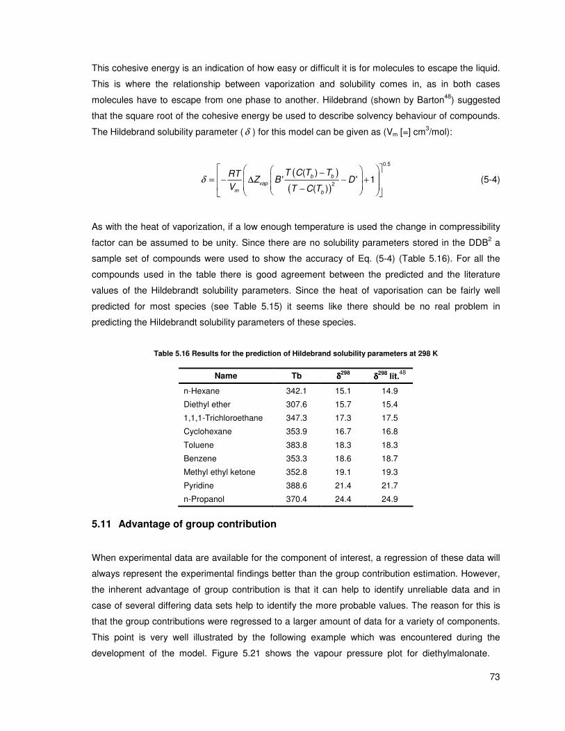
73

This cohesive energy is an indication of how easy or difficult it is for molecules to escape the liquid.

This is where the relationship between vaporization and solubility comes in, as in both cases

molecules have to escape from one phase to another. Hildebrand (shown by Barton48

) suggested

that the square root of the cohesive energy be used to describe solvency behaviour of compounds.

The Hildebrand solubility parameter (δ ) for this model can be given as (Vm [=] cm3/mol):

( )

( )

0.5

2

( )' ' 1

( )

b b

vap

m b

T C T TRTZ B D

V T C Tδ

− = − ∆ − +

−

(5-4)

As with the heat of vaporization, if a low enough temperature is used the change in compressibility

factor can be assumed to be unity. Since there are no solubility parameters stored in the DDB2 a

sample set of compounds were used to show the accuracy of Eq. (5-4) (Table 5.16). For all the

compounds used in the table there is good agreement between the predicted and the literature

values of the Hildebrandt solubility parameters. Since the heat of vaporisation can be fairly well

predicted for most species (see Table 5.15) it seems like there should be no real problem in

predicting the Hildebrandt solubility parameters of these species.

Table 5.16 Results for the prediction of Hildebrand solubility parameters at 298 K

Name Tb δδδδ298

δδδδ298

lit.48

n-Hexane 342.1 15.1 14.9

Diethyl ether 307.6 15.7 15.4

1,1,1-Trichloroethane 347.3 17.3 17.5

Cyclohexane 353.9 16.7 16.8

Toluene 383.8 18.3 18.3

Benzene 353.3 18.6 18.7

Methyl ethyl ketone 352.8 19.1 19.3

Pyridine 388.6 21.4 21.7

n-Propanol 370.4 24.4 24.9

5.11 Advantage of group contribution

When experimental data are available for the component of interest, a regression of these data will

always represent the experimental findings better than the group contribution estimation. However,

the inherent advantage of group contribution is that it can help to identify unreliable data and in

case of several differing data sets help to identify the more probable values. The reason for this is

that the group contributions were regressed to a larger amount of data for a variety of components.

This point is very well illustrated by the following example which was encountered during the

development of the model. Figure 5.21 shows the vapour pressure plot for diethylmalonate.

74

Judging from the regression curve there is a significant scatter in the data. However the predicted

curve reveals that the low pressure data must be erroneous

-4.5

-4

-3.5

-3

-2.5

-2

-1.5

-1

-0.5

0

0.002 0.0021 0.0022 0.0023 0.0024 0.0025 0.0026

1/T (K-1)

ln(P

s/1

01

.3 k

Pa

)

Figure 5.21 ln(Ps/101.3kPa) vs. 1/T for diethyl malonate (x – data taken from the DDB

2,

____ predicted, - - - - fitted)

5.12 General results and discussion

The vapour pressure percentage error for all compounds was found to be 5.0% (2332 compounds

113 888 data points) which compares very favourably to the method of Nannoolal which has an

error of 6.6 % (2207 compounds 111 757 data points). As can be seen from Table 5.17 the greatest

improvement is for pressures below 10 kPa (LP & ELP) where the percentage error is much lower

than it was previously. For pressures above 10 kPa there is still an improvement but not nearly as

noticeable as for the lower pressures. As the normal boiling temperature is supplied as a

parameter, huge deviations in B’ are required to produce larger errors in vapour pressure in the

vicinity of atmospheric pressure. Therefore the improvement in case of low pressure data far away

from the reference point is a sensible measure of model performance.

Table 5.17 Relative mean deviation [%] in vapour pressure estimation for the new method and the method of

Nannoolal et al. The number in superscript is the number of data points used; the main number is the average

percentage error of each data point. NC – Number of compounds; ELP – Extremely low pressure P < 10 Pa; LP –

Low pressure 10 Pa 500 kPa;

AVE – Average error.


All compounds (this work) 2332 25.7 2211

9.8 28232

2.3 68729

5.0 14678

5.0 113887

All compounds (Nannoolal et al.) 2207 55.2 2205

13.1 27687

2.6 67518

5.7 14310

6.6 111757

75

In the sections preceding there has been very little mention of the chance of failure of the model

(i.e. compounds with an unacceptably high vapour pressure – e.g. > 20% RMD). The reason for this

is that there were only very few compounds which failed. Figure 5.22 shows that the vast majority of

the data (85%) lies under the 10% RMD mark. The compounds with a RMD above 10% (or more

specifically 10 – 20 %) are almost all there due to slightly lower quality data. Many compounds

which are above the 20% RMD (4% of the total data) are a combination of suspect data (many have

<10 data points from only one source) and genuine failure of the method. The best example of

failure is with glycols (e.g. triethylene glycol). Even with the special attention that has been given to

the alcohols, the glycols are still very difficult to predict accurately. Similarly, diols with other non –

hydrocarbon groups (e.g. ethylene nitrate – 40% RMD) are also quite difficult to accurately predict

(some attention was given to this in paragraph 5.7). While any error greater than 20% is not great it

can still be useful if a rough vapour pressure estimate is needed, and it is useful to note that there

were no errors exceeding 60% RMD.

0

100

200

300

400

500

600

700

800

900

0 - 2 2 - 5 5 - 10 10 - 15 15 - 20 20 - 40 40 - 60 >60

RMD (%)

Nu

mb

er

of

Co

mp

ou

nd

s

Figure 5.22 Histogram of the vapour pressure relative mean deviation for the compounds in the training set

A total of 212 groups were used to describe the data (both group interaction and group contribution

groups), however some groups have only been regressed against 1 or 2 compounds and therefore

should only be used as a guide when applied. The group contribution and interaction tables are

given in Appendix A. Since there is such a large improvement in the low pressure predictions the

model could be used to extrapolate to the normal boiling temperature from low pressure data.

76

This would be quite a logical application as there are a number of low pressure data available for

compounds which do not have a measured boiling point. The drawback of a method such as this is

that the extrapolation would only be as good as the data it was extrapolated from, and since low

pressure data often has a large amount of scatter this could prove problematic. It is therefore

recommended that any boiling point extrapolations be used in conjunction with some of the more

conventional boiling point estimation methods available (Rarey et al.5 and Nannoolal et al.

6).

77

6 CONCLUSIONS

An improved group contribution method has been developed for the prediction of vapour pressures.

The group contribution scheme employed by Nannoolal et al. was modified to account for the size

dependence of some groups that were found in the development of the model. This allows for the

improved prediction of these groups (most noticeable were the aliphatic alcohols, aliphatic

carboxylic acids and ketones). The C-parameter used by Nannoolal et al.8 was also modified in

order to account for a wider range of molecule sizes and to increase the prediction of the vapour

pressure model at low pressures. A large improvement in the predictions of the aliphatic alcohol

and aliphatic carboxylic acid groups was made by adding in a logarithmic correction term which

provides a more physically realistic shape of the curve.

A training set of 2332 compounds (113 888 data points) was used in the development of the model

and an average percentage error of 5.0% was found. This compares favourably with the method of

Nannoolal et al.8 was for 2207 compounds and 111 757 data points had an average percentage

error of 6.6 %. The largest improvement was at low pressures (<10 kPa) where the error is almost

half of that obtained by the method of Nannoolal et al.8. This large improvement is a sensible

measure of the performance of the model since the low pressure data are very far from the datum

point (which is the normal boiling point).

In order to test the performance of the model (to make sure it was not simply well trained to the data

used in the model development) a test set of data, heat of vaporization data at 298 K and solid

vapour pressure data were used. The average percentage error for each vapour pressure point in

the test set was found to be 7.1 %, which was a bit inflated due to the large amount of scatter that

was observed in the test data. The average percentage error for the heat of vaporization data at

298 K was 3.5% which shows that the model parameters are both accurate and physically realistic.

For the solid vapour pressure data the average percentage error for each data point was found to

be 21.1%; again this was a bit inflated due to the large amount of scatter present in the low

pressure data.

78

7 RECOMMENDATIONS

This work is a continuation of an ongoing project for the prediction of thermophysical properties

using group contribution. The properties that have so far been successfully predicted with much

acclaim are (all for non-electrolytic organic compounds):

• The normal boiling point

• The critical temperature, pressure and volume

• Viscosity

• Vapour pressure (which was improved in this work)

There are still are a huge amount of properties which could be predicted, and with the continual

improvement of the software and group definition (through works such as this and Nannoolal et al.)

the methods should continue to improve. Some thermophysical properties which could be of

interest are:

• Solvent solubility

• Surface tension

• Thermal conductivity

• Melting temperature

The power of group contribution methods is that the model parameters can be predicted from the

molecular structure. In this method, for example, it is preferable to have experimental boiling point

data but if there is none available it can be predicted from methods currently available5,6

. This will

obviously affect the accuracy of the prediction but it does mean that a vapour pressure curve can

be generated by only knowing the molecular structure.

79

8 REFERENCES

1 Daubert, T. E., Strengths and Weaknesses of Predictive Methods for Estimating Thermophysical

Properties., J. Chem. Eng. Data 41 (1996) 942.

2 Gmehling, J., Rarey, J., Menke, J., Dortmund Data Bank, Oldenburg (2007) http://www.ddbst.com.

3 Environmental news network, www.enn.com, last accessed 20 July 2007.

4 Bowen, H. J., Palmer, S. R., Fielder, H. M., Coleman, G., Routledge, P. A., Fone, D. L.,

Community exposures to chemical incidents: Europe environmental public health surveillance

system in development and evaluation of the first., Jech Online (jech.bmj.com), last accessed 20

July 2007.

5 Rarey, J., Cordes, W., A New Method for the Estimation of the Normal Boiling Point of Non-

Electrolyte Organic Compounds., Fluid Phase Equilibria, 201 (2002) 409.

6 Nannoolal, Y., Rarey, J., Ramjugernath, D., Cordes, W., Estimation of Pure Component

Properties, Part 1: Estimation of the Normal Boiling Point of Non-Electrolyte Organic Compounds

via Group Contributions and Group Interactions., Fluid Phase Equilib., 226 (2004) 45-63.

7 Nannoolal, Y., Rarey, J., Ramjugernath, D., Estimation of Pure Component Properties Part 2:

Estimation of Critical Data by Group Contribution., Fluid Phase Equilib., 252 (2007) 1.

8 Nannoolal, Y., Rarey, J., Ramjugernath, D., Estimation of Pure Component Properties Part 3:

Estimation of the Vapor Pressure of Non-Electrolyte Organic Compounds via Group Contributions

and Group Interactions., Fluid Phase Equilib. submitted for publication.

9 Wagner, W., A New Correlation Method for Thermodynamic Data Applied to the Vapor Pressure

Curve on Argon, Nitrogen and Water. London: IUPAC Thermodynamic Tables Project Centre.

(1977).

10 Antoine, C., Vapor Pressure: A New Relation between Vapor Pressure and Temperature.,

Compt. Rend. 107 (1888a) 836.

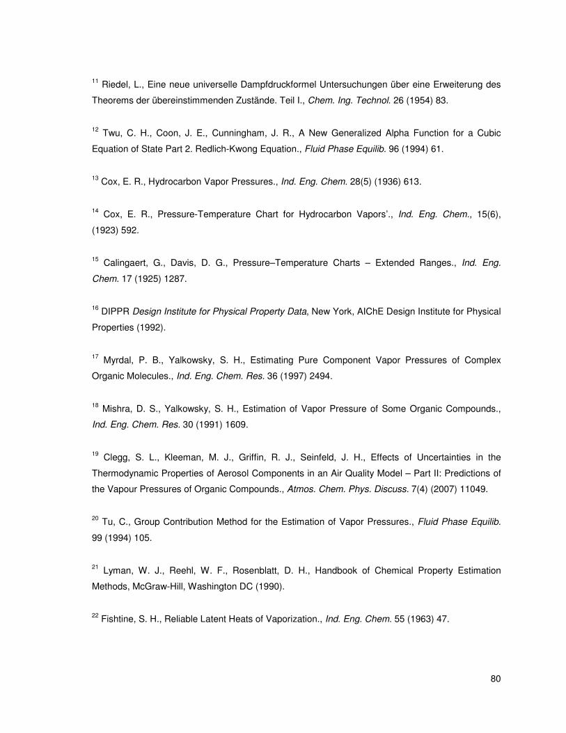
80

11 Riedel, L., Eine neue universelle Dampfdruckformel Untersuchungen über eine Erweiterung des

Theorems der übereinstimmenden Zustände. Teil I., Chem. Ing. Technol. 26 (1954) 83.

12 Twu, C. H., Coon, J. E., Cunningham, J. R., A New Generalized Alpha Function for a Cubic

Equation of State Part 2. Redlich-Kwong Equation., Fluid Phase Equilib. 96 (1994) 61.

13 Cox, E. R., Hydrocarbon Vapor Pressures., Ind. Eng. Chem. 28(5) (1936) 613.

14 Cox, E. R., Pressure-Temperature Chart for Hydrocarbon Vapors’., Ind. Eng. Chem., 15(6),

(1923) 592.

15 Calingaert, G., Davis, D. G., Pressure–Temperature Charts – Extended Ranges., Ind. Eng.

Chem. 17 (1925) 1287.

16 DIPPR Design Institute for Physical Property Data, New York, AIChE Design Institute for Physical

Properties (1992).

17 Myrdal, P. B., Yalkowsky, S. H., Estimating Pure Component Vapor Pressures of Complex

Organic Molecules., Ind. Eng. Chem. Res. 36 (1997) 2494.

18 Mishra, D. S., Yalkowsky, S. H., Estimation of Vapor Pressure of Some Organic Compounds.,

Ind. Eng. Chem. Res. 30 (1991) 1609.

19 Clegg, S. L., Kleeman, M. J., Griffin, R. J., Seinfeld, J. H., Effects of Uncertainties in the

Thermodynamic Properties of Aerosol Components in an Air Quality Model – Part II: Predictions of

the Vapour Pressures of Organic Compounds., Atmos. Chem. Phys. Discuss. 7(4) (2007) 11049.

20 Tu, C., Group Contribution Method for the Estimation of Vapor Pressures., Fluid Phase Equilib.

99 (1994) 105.

21 Lyman, W. J., Reehl, W. F., Rosenblatt, D. H., Handbook of Chemical Property Estimation

Methods, McGraw-Hill, Washington DC (1990).

22 Fishtine, S. H., Reliable Latent Heats of Vaporization., Ind. Eng. Chem. 55 (1963) 47.

81

23 Voutsas, E., Lampadariou, M., Magoulus, K., Tassios, D., Prediction of Vapor Pressures of Pure

Compounds from Knowledge of the Normal Boiling Point Temperature., Fluid Phase Equilib. 198

(2002) 81.

24 Abrams, D. S., Massaldi, H. A., Prausnitz J. M., Vapor Pressures of Liquids as a Function of

Temperature. Two-Parameter Equation Based on Kinetic Theory of Fluids., Ind. Eng. Chem.

Fundam. 13(3) (1974) 259.

25 Moelwyn-Hughes, E. A., The Chemical Statics and Kinetics of Solutions, Academic Press,

London (1971).

26 Soave, G., Equilibrium Constants from a Modified Redlich-Kwong Equation of State., Chem. Eng.

Sci. 27 (1972) 1197.

27 Coquelet, C., Chapoy, A., Richon, D., Development of a New Alpha Function for the Peng–

Robinson Equation of State: Comparative Study of Alpha Function Models for Pure Gases (Natural

Gas Components) and Water-Gas Systems., Int. J. Thermophysics 25(1) (2004) 133.

28 Copeman, T. W., Mathias, P. M., Vapor pressures of pure compounds using the Peng–Robinson

equation of state with three different attractive terms., Fluid Phase Equilib. 13 (1983) 59.

29 Reid, R. C., Prausnitz, J. M., Poling, B. E., The Properties of Gases and Liquids, 4

th Ed.,

McGraw-Hill, USA (1987).

30 Eubank, P. T., Wang, X., Saturation Properties from Equations of State., Ind. Eng. Chem. Res.

42 (2003) 3838.

31 Hanif, N. S. M., Shyu, G., Hall, K. R., Eubank, P. T., Areas of J. C. Maxwell for Pure-Component

Fluid-Phase Equilibria from Equations of State., Ind. Eng. Chem. Res. 35 (1996) 2431.

32 Pitzer, K. S., Lippmann, D. Z., Curl, R. F., Huggins, C. M., Petersen, D. E., The Volumetric and

Thermodynamic Properties of Fluids. II. Compressibility Factor, Vapor Pressure and Entropy of

Vaporization., J. Am. Chem. Soc. 77 (1955) 3433.

33 Lee, B. I., Kesler, M. G., A Generalized Thermodynamic Correlation Based on Three-Parameter

Corresponding States., AIChE J. 21 (1975) 137.

82

34 Thomson, G. W., The Antoine Equation for Vapor-Pressure Data., Chemical Reviews 38(7)

(1946) 1.

35 Ambrose, D., J. The correlation and estimation of vapour pressures IV. Observations on

Wagner's method of fitting equations to vapour pressures., Chem. Thermodynamics 18 (1986) 45.

36 Chase, D. J., Two Models of Vapor Pressure along the Saturation Curve Ind. Eng. Chem. Res.

26 (1987) 107.

37 Waring, W., Form of a Wide-Range Vapor Pressure Equation., Ind. Eng. Chem. 46(4) (1954) 762.

38 Liang, C., Gallagher, D. A., QSPR Prediction of Vapor Pressure from Solely Theoretically-Derived

Descriptors., J. Chem. Inf. Comp. Sci. 38(2) (1998) 321.

39 Paul, P. K., Prediction of vapour pressure using descriptors derived from molecular dynamics.,

Org. Biomol. Chem. 3 (2005) 1176.

40 Ambrose D., Vapor-Pressure Equations. National Physical Laboratory NPL Rep. Chem, 114

(1980).

41 Ledanois, J., Colina, C. M., Santos, J. W., Gonzalez-Mendizabel, D., Olivera-Fuentes, C., Ind.

Eng. Chem. Res. 36 (1997) 2505.

42 Ben-Naim, A., Solvation Thermodynamics, Plenum Press (1987).

43 Lin, S., Chang, J., Wang, S., Goddard, W. A., Sandler, S. I., Prediction of Vapor Pressures and

Enthalpies of Vaporization Using a COSMO Solvation Model., J. Phys. Chem. 108 (2004) 7429.

44 Press et al., Numerical Recipes in Fortran the Art of Scientific Computing, 2

nd Ed., Cambridge

University Press (1986).

45 Dennis, J. E., Schnabel R. B., Numerical Methods for Unconstrained Optimization of Nonlinear

Equations, Prentice-Hall, New York (1983).

83

46 Lampton, M., Damping-Undamping Strategies for the Levenberg-Marquardt Nonlinear. Least-

Squares Method., Computers in Physics 11(1) (1997) 110.

47 Cordes et al., Software Development in Chemistry 7, Proceding of the Computer in Chemie 7,

Paper presented at the D. Ziessow (Ed.), Springer-Verlag, Berlin (1993).

48 Barton, A. F., Handbook of Solubility Parameters and Other Cohesion Parameters, 2

nd Ed., CRC

Press, USA (1991).

84

APPENDICES

A GROUP CONTRIBUTION AND INTERACTION TABLES

Table A.1 Group contribution and group interaction values and descriptions

Ink No

Name Description dBi Example Prty Size Dep

Ref No

- A The constant term A 9.42208 - - - -

ALIPHATIC CARBON GROUPS

1 -CH3 Methyl group attached to a non-aromatic non-electronegative atom

-0.00227 2,2-Dimethylbutane 135 No 101

4 -CH2- CH2 in a chain 0.07545 n-Butane 141 No 102

5 >CH- CH in a chain 0.07099 3-Ethylpentane 144 No 103

6 >C< C in a chain -0.04707 2,2,4-Trimethylpentane 146 No 104

2 -CH3 Methyl group attached to a non-aromatic electronegative atom

0.13491 N-Methylaniline 132 No 105

7 -CH2- CH2 in a chain attached to an electronegative atom

0.11758 Ethylenediamine 136 No 106

8 -CH< CH in a chain attached to an electronegative atom

0.08955 5-Ethyl-2-nonanol 137 No 107

9 >C< C in a chain attached to an electronegative atom

-0.08960 tert-Butanol 138 No 108

29 -CH3 Methyl group attached to a ring carbon -0.07834 Methylcyclohexane 122 No 109

10 -CH2- CH2 in a ring -0.01350 Cyclohexane 143 No 110

11 >CH- CH in a ring 0.06029 Methylcyclohexane 145 No 111

12 >C< C in a ring 0.10842 1,1-Dimethylcyclopentane 147 No 112

131 >CH(r) - C(r)<

CH in a ring bonded to a carbon in a different ring

0.01296 cis-Decahydronaphthalene

110 No 113

136 C(k)-C(r)-3C(r)

Ring carbon attached to 3 other ring carbons and a chain carbon

0.00823 1,3-Dimethyl adamantane 108 No 114

137 C-4C(r) Ring carbon attached to 4 other ring carbons

0.17344 Spiro[4.5]decane 109 No 115

24 -CH2(r)-en CH2 in a ring attached to an electronegative carbon

0.08201 1,4-Dioxane 142 No 116

14 >CH- CH in a ring attached to an electronegative atom

0.10344 Cyclopentanol 139 No 117

15 >C< C in a ring attached to an electronegative atom

-0.12395 Perfluorocyclopentane 140 No 118

139 C(r)_3C(r)_en

Ring carbon bonded to 3 other ring carbons and an en atom

-0.05881 1-Nitroadamantane 107 No 119

85

Ink No


Ref No

26 CH2= Double bonded carbon at the end of a chain/ring

-0.00564 1-Nonene 117 Yes 120

20 -CH=C- Double bonded carbon in a chain with only 1 carbon neighbour

0.00286 2-Heptene 121 Yes 121

27 -C=C- Double bonded carbon in a chain with 2 carbon neighbours

0.00475 2-Methyl-2-pentene 118 Yes 122

31 >C=C=C< C=C=C; cumulated double bonds 0.08031 1,2-Butadiene 112 Yes 123

33 >C=C-C=C<

C=C-C=C (chain); conjugated double bonds (chain)

0.03953 trans-1,3-Pentadiene 114 Yes 124

21 >C=C< Double bond between carbons in a ring 0.00242 1,3-Cyclopentadiene 123 Yes 125

13 -C=C< Double bonded carbon in a ring with 2 carbon neighbours

0.02664 1-Methylcyclohexene 120 Yes 126

32 >C=C-C=C<

C=C-C=C (ring); conjugated double bonds (ring)

-0.00045 1,3-Cyclopentadiene 113 Yes 127

134 >C(r)=C(k) Carbon in a ring double bonded to a carbon outside the chain

0.01488 beta-Pinene 106 Yes 128

25 CH# Carbon triple bonded to another carbon at the end of a chain

-0.03884 1-Octyne 124 Yes 129

22 -CtC- Triple bond between 2 carbons in a chain -0.01491 2-Heptyne 125 Yes 130

34 -C#C-C#C- C#C-C#C; conjugated triple bonds 0.00977** 2,4-Hexadiyne 111 Yes 131

AROMATIC CARBON GROUPS

3 -CH3 Methyl group attached to an aromatic atom

-0.01001 1-Methyl naphthalene 133 No 201

16 -CH(a)< CH in an aromatic ring 0.01653 Benzene 128 No 202

17 >C(a)< C in an aromatic ring 0.11192 Propylbenzene 131 No 203

19 =C(a)< Aromatic carbon attached to three aromatic neighbours

-0.01113 Naphthalene 116 No 204

132 C(a)-C(r) < Aromatic carbon bonded to a carbon in a ring

0.07303 1,2,3,4-Tetrahydronaphthalene

129 No 205

133 C(a)-C(a) 2 Aromatic carbons chain bonded 0.13938 Benzidine 130 No 206

135 C(a)-r-C(a) Aromatic carbon bonded to an aromatic carbon in a ring

-0.10703 9H-Fluorene 115 No 207

138 C(a)-C= Aromatic carbon attached to a double bonded carbon

0.26362 Divinylbenzene 127 No 208

18 >C(a)< C in an aromatic ring attached to an electronegative atom

0.21038 Aniline 119 No 209

FLUORINE GROUPS

35 F- Fluorine attached to non-aromatic carbon 0.06101 1-Fluoropentane 92 No 301

38 F-C-1Halo Fluorine attached to a carbon with one other halogen atom

0.10540 Perfluorocyclopentane 71 No 302

86

Ink No


Ref No

39 F-C-2Halo Fluorine attached to a carbon with two other halogen atoms

0.09402 1,1,1,2-Tetrachloro-2,2-difluoroethane [R112a]

70 No 303

36 F-C= Fluorine attached to double bonded carbon

0.11304 2-Fluoropropane 69 No 304

148 F-C=(1 Halo)

Fluorine attached to a double bonded carbon with one other halogen atom

0.07386 1,1-Difluoroethene 68 No 305

37 F-C(a) Fluorine attached to aromatic carbon -0.07045 Fluorobenzene 91 No 306

116 Fe-Si< Fluorine attached to a silicon atom 0.21389 Silicon tetrafluoride 1 No 307

CHLORINE GROUPS

40 Cl- Chlorine attached to non-aromatic carbon 0.06508 Chloroethane 76 No 401

43 Cl-C-1Halo Chlorine attached to a carbon with one other halogen atom

0.03302 2-Bromo-2-chloro-1,1,1-trifluoroethane

67 No 402

44 Cl-C-2Halo Chlorine attached to a carbon with two other halogen atoms

0.05138 1,1,1-Trichloroethane [R140a]

66 No 403

42 Cl-C= Chlorine attached to double bonded carbon

0.07694 2-Chloro-1,3-butadiene 65 No 404

149 Cl-C=(1 Halo)

Chlorine attached to a double bonded carbon with one other halogen atom

0.12660 Tetrachloroethylene 64 No 405

41 Cl-C(a) Chlorine attached to aromatic carbon -0.19988 Chlorobenzene 77 No 406

117 Cl-Si< Chlorine attached to a silicon atom -0.00761 Trichlorosilane 2 No 407

113 COCl- Acid chloride 0.33205 Trichloroacetyl chloride 19 No 408

BROMINE GROUPS

45 Br- Bromine attached to non-aromatic carbon -0.01712 1,2-Dibromoethane 78 No 501

144 Br-C-1Halo Bromine attached to a carbon with one other halogen atom

0.07426 2-Bromo-2-chloro-1,1,1-trifluoroethane

75 No 502

145 Br-C-2Halo Bromine attached to a carbon with two other halogen atom

-0.02594 Tribromomethane [R20B3]

74 No 503

146 Br-C= Bromine attached to a double bonded carbon

0.15186 Vinyl bromide 73 No 504

46 Br-C(a) Bromine attached to aromatic carbon -0.18810 Bromobenzene 79 No 506

118 Br-Si< Bromine attached to a silicon atom -0.13300 Silicon tetrabromide 3 No 507

IODINE GROUPS

47 I- Iodine attached to carbon 0.02257 Ethyl iodide 61 No 601

119 I-Si< Iodine attached to a silicon atom 1.30968** Triiodomethylsilane 4 No 607

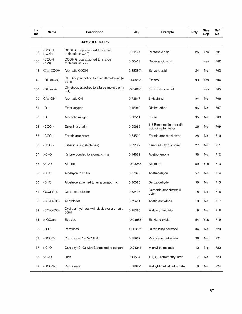
87

Ink No


Ref No

OXYGEN GROUPS

53 -COOH (n=<9)

COOH Group attached to a small molecule (n =< 9)

0.81104 Pentanoic acid 25 Yes 701

155 -COOH (n>9)

COOH Group attached to a large molecule (n > 9)

0.08469 Dodecanoic acid Yes 702

48 C(a)-COOH Aromatic COOH 2.38380* Benzoic acid 24 No 703

49 -OH (n=<4) OH Group attached to a small molecule (n =< 4)

-0.43267 Ethanol 93 Yes 704

153 -OH (n>4) OH Group attached to a large molecule (n > 4)

-0.04696 5-Ethyl-2-nonanol Yes 705

50 C(a)-OH Aromatic OH 0.73847 2-Naphthol 94 No 706

51 -O- Ether oxygen 0.15049 Diethyl ether 96 No 707

52 -O- Aromatic oxygen 0.23511 Furan 95 No 708

54 -COO - Ester in a chain 0.55698 1,3-Benzenedicarboxylic acid dimethyl ester

26 No 709

55 -COO - Formic acid ester 0.54599 Formic acid ethyl ester 28 No 710

56 -COO - Ester in a ring (lactones) 0.53129 gamma-Butyrolactone 27 No 711

57 >C=O Ketone bonded to aromatic ring 0.14889 Acetophenone 58 No 712

58 >C=O Ketone -0.03266 Acetone 59 Yes 713

59 -CHO Aldehyde in chain 0.37695 Acetaldehyde 57 No 714

60 -CHO Aldehyde attached to an aromatic ring 0.20025 Benzaldehyde 56 No 715

61 O=C(-O-)2 Carbonate diester 0.52435 Carbonic acid dimethyl ester

15 No 716

62 -CO-O-CO- Anhydrides 0.79451 Acetic anhydride 10 No 717

63 -CO-O-CO- Cyclic anhydrides with double or aromatic bond

0.95360 Maleic anhydride 9 No 718

64 >(OC2)< Epoxide -0.08988 Ethylene oxide 54 Yes 719

65 -O-O- Peroxides 1.90315* Di-tert.butyl peroxide 34 No 720

66 -OCOO- Carbonates O-C=O & -O 0.55927 Propylene carbonate 36 No 721

67 >C=O Carbonyl(C=O) with S attached to carbon -0.28344* Methyl thioacetate 42 No 722

68 >C=O Urea 0.41594 1,1,3,3-Tetramethyl urea 7 No 723

69 -OCON< Carbamate 3.68627* Methyldimethylcarbamate 6 No 724

88

Ink No


Ref No

NITROGEN GROUPS

70 -CONH< Amide with no substituents 2.15987* Acetamide 29 No 801

71 -CONH< Amide with one substituent attached to the nitrogen

1.56627 N-Methylformamide 11 No 802

72 -CONH< Amide with two substituents attached to the nitrogen

0.46886 N,N-Dimethylformamide (DMF)

12 No 803

73 OCN- Isocyanate 0.19547 Isocyanic acid methyl ester

31 Yes 804

141 -OCN(a) IsoCyanate attached to an aromatic carbon

0.49979 Phenyl isocyanate 30 No 805

74 ONC- Oxime 2.55684 Methyl ethyl ketoxime 32 No 806

75 NO2- Nitro group attached to a non-aromatic carbon

0.32934 Nitromethane 21 No 807

76 NO2- Nitro group attached to an aromatic carbon

0.22620 Nitrobenzene 22 No 808

77 NO2- Nitrite -0.28378** Ethyl nitrite 23 No 809

78 -ON= Isoxazole O-N=C 0.52969* 5-Methyl-4-nitroisoxazole 51 No 810

79 NO3- Nitrate 0.83647 Ethylnitrate 14 No 811

80 NH2- Primary amine attached to non-aromatic carbon/silicon

-0.05329 Ethylenediamine 98 Yes 812

81 NH2- Primary amine attached to aromatic carbon

0.33218 Aniline 97 No 813

82 -NH- Secondary amines (chain) attached to carbons/silicons

0.41210 Dibutylamine 102 No 814

86 =N- Secondary amines (chain) attached to one carbons/silicons via double bond

0.82998 N-Benzylidenemethyl amine

105 No 815

93 -NH- Secondary amines (ring) attached to carbons/silicons

0.58897 Morpholine 101 No 816

94 -NH- secondary amines attached to aromatic carbons/silicons

0.30756 N-Methylaniline 33 No 817

84 -N< Tertiary amine attached to carbons/silicons

-0.22437 N,N-dimethylaniline 104 No 818

92 -N< tertiary amines attached to aromatic carbon

0.07255 N,N-Dimethylaniline 43 No 819

85 >N< Nitrogen attached to four carbons -1.17553* N,N,N',N'-Tetramethylmethylenediamine

35 No 820

140 C2-N-C(r) Cyclic tertiary amines -0.28632 N-Methylpiperidine 103 No 820

83 N=N Azene N=N 0.00256 Azobenzene 50 No 821

130 >N-N< A hydrazine functional group 0.96678 Hydrazine 49 No 822

143 N-N_C Hydrazine with 1 carbon neighbours 0.71254 Phenylhydrazine 48 No 823

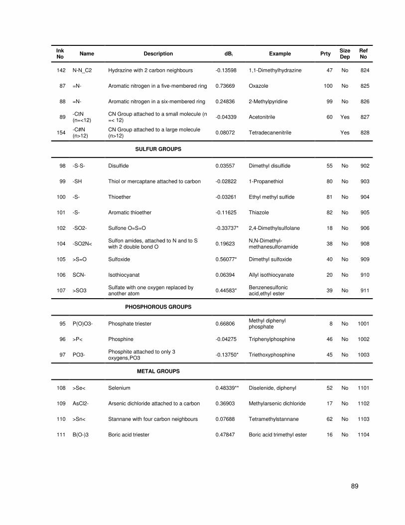
89

Ink No


Ref No

142 N-N_C2 Hydrazine with 2 carbon neighbours -0.13598 1,1-Dimethylhydrazine 47 No 824

87 =N- Aromatic nitrogen in a five-membered ring 0.73669 Oxazole 100 No 825

88 =N- Aromatic nitrogen in a six-membered ring 0.24836 2-Methylpyridine 99 No 826

89 -CtN (n=<12)

CN Group attached to a small molecule (n =< 12)

-0.04339 Acetonitrile 60 Yes 827

154 -C#N (n>12)

CN Group attached to a large molecule (n>12)

0.08072 Tetradecanenitrile Yes 828

SULFUR GROUPS

98 -S-S- Disulfide 0.03557 Dimethyl disulfide 55 No 902

99 -SH Thiol or mercaptane attached to carbon -0.02822 1-Propanethiol 80 No 903

100 -S- Thioether -0.03261 Ethyl methyl sulfide 81 No 904

101 -S- Aromatic thioether -0.11625 Thiazole 82 No 905

102 -SO2- Sulfone O=S=O -0.33737* 2,4-Dimethylsulfolane 18 No 906

104 -SO2N< Sulfon amides, attached to N and to S with 2 double bond O

0.19623 N,N-Dimethyl-methanesulfonamide

38 No 908

105 >S=O Sulfoxide 0.56077* Dimethyl sulfoxide 40 No 909

106 SCN- Isothiocyanat 0.06394 Allyl isothiocyanate 20 No 910

107 >SO3 Sulfate with one oxygen replaced by another atom

0.44583* Benzenesulfonic acid,ethyl ester

39 No 911

PHOSPHOROUS GROUPS

95 P(O)O3- Phosphate triester 0.66806 Methyl diphenyl phosphate

8 No 1001

96 >P< Phosphine -0.04275 Triphenylphosphine 46 No 1002

97 PO3- Phosphite attached to only 3 oxygens,PO3

-0.13750* Triethoxyphosphine 45 No 1003

METAL GROUPS

108 >Se< Selenium 0.48339** Diselenide, diphenyl 52 No 1101

109 AsCl2- Arsenic dichloride attached to a carbon 0.36903 Methylarsenic dichloride 17 No 1102

110 >Sn< Stannane with four carbon neighbours 0.07688 Tetramethylstannane 62 No 1103

111 B(O-)3 Boric acid triester 0.47847 Boric acid trimethyl ester 16 No 1104

90

Ink No


Ref No

GERMANIUM GROUPS

114 GeCl3- GeCl3 attached to carbon 0.27066 Trichlorosilyl(trichlorogermyl)methane

13 No 1201

115 >Ge< Germane with four carbon neighbors 0.34203 Tetramethylgermane 63 No 1202

SILICON GROUPS

120 -SiH3 Silane group -0.24084 Butylsilane 84 No 1301

121 -SiH2- Primary silicon group 0.27568 Trisilane 88 No 1302

122 -SiH< Secondary silicon group -0.29038 Triethylsilane 89 No 1303

123 >Si< Tertiary silicon group 0.03614 Tetraethylsilane 90 No 1304

124 -SiH3 Silane group attached to an electromagnetic atom

0.20445 Monochlorosilane 83 No 1305

127 SiH2 SiH2 attached to electronegative atoms 0.21195 Dichlorosilane 85 No 1306

128 SiH SiH attached to electronegative atoms -0.01409 Trichlorosilane 86 No 1307

125 >Si< Silicon atom bonded to electromagnetic atoms

0.03880 Tetrachlorosilane 87 No 1308

129 CH3-Si Methyl group attached to a Silicon atom -0.00451 Tetramethylsilane 134 No 1309

SPECIAL GROUPS

150 no H No hydrogen atoms -0.19373 Perfluoropentane No 1401

151 one H One hydrogen atom -0.04327 2-Bromo-2-chloro-1,1,1-trifluoroethane

No 1402

SIZE DEPENDANT GROUP

CONSTANTS

170 Alkenes group constant -0.02835 No 2001

171 Alkynes group constant 0.60141 No 2002

172 Ketone group constant 0.71345 No 2003

173 Epoxy group constant 0.91912 No 2004

174 Isocyanate group constant -0.41147 No 2005

175 Short OH group constant (n=<4) 6.69345 No 2006

176 Long OH group constant (n>4) 5.21138 No 2007

177 Primary amine group constant 0.91589 No 2008

91

Ink No


Ref No

179 Short CN group constant (n=<12) 0.61103 No 2010

180 Long CN group constant (n>12) -1.05206 No 2011

181 Short COOH group constant (n=<9) -2.54299 No 2012

182 Long COOH group constant (n>9) 3.92217 No 2013

GROUP INTERACTIONS

200 Alcohol - Alcohol Interaction -0.00306 Yes 3001

201 Alcohol - 1 Amine Interaction -0.26016 No 3002

202 Alcohol - 2 Amine Interaction -0.50269 No 3003

203 Alcohol - Thiol Interaction -1.13734* No 3004

205 Alcohol - Ether Interaction -0.55743 No 3006

207 Alcohol - Ester Interaction -1.38632 No 3008

208 Alcohol - Ketone Interaction -1.38783** No 3009

210 Alcohol - Cyan Interaction 0.13770* No 3011

220 1 Amine - 1 Amine Interaction 0.82184 No 3021

221 1 Amine - 2 Amine Interaction -0.29523** No 3022

224 1 Amine - Ether Interaction 0.07904 No 3025

226 1 Amine - Ester Interaction -0.80854* No 3027

230 1 Amine - Aromatic O Interaction -0.75793* No 3031

232 1 Amine - Alcohol (a) Interaction 2.06766* No 3033

237 1 Amine - Nitro(a) Interaction 0.06456 No 3038

239 2 Amine - 2 Amine Interaction -0.23506** No 3040

242 2 Amine - Ether Interaction -0.05391* No 3043

257 Thiol - Thiol Interaction 0.46453 No 3058

267 Thiol - Alcohol (a) Interaction 0.24272* No 3068

274 Carboxy - Carboxy Interaction -2.42076 No 3075

286 Carboxy - Aromatic S Interaction -1.67665* No 3087

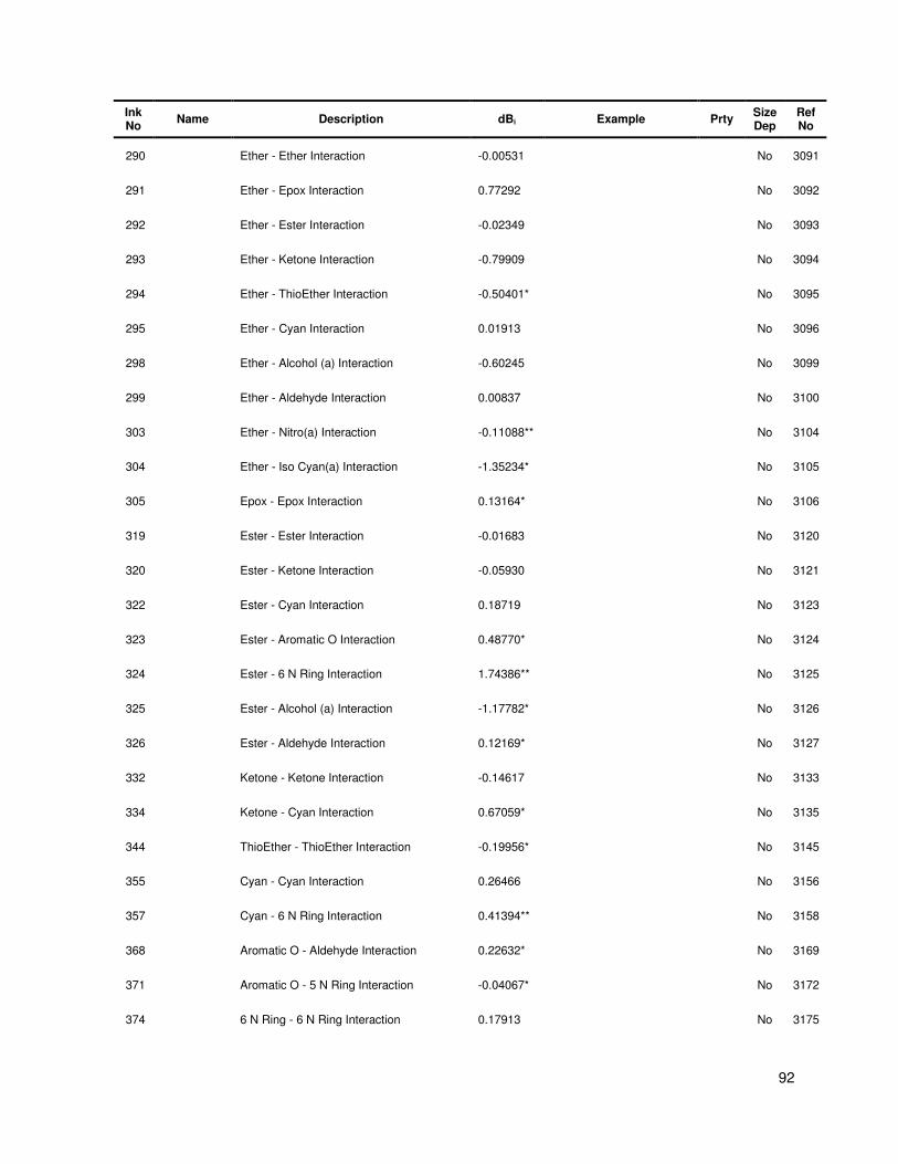
92

Ink No


Ref No

290 Ether - Ether Interaction -0.00531 No 3091

291 Ether - Epox Interaction 0.77292 No 3092

292 Ether - Ester Interaction -0.02349 No 3093

293 Ether - Ketone Interaction -0.79909 No 3094

294 Ether - ThioEther Interaction -0.50401* No 3095

295 Ether - Cyan Interaction 0.01913 No 3096

298 Ether - Alcohol (a) Interaction -0.60245 No 3099

299 Ether - Aldehyde Interaction 0.00837 No 3100

303 Ether - Nitro(a) Interaction -0.11088** No 3104

304 Ether - Iso Cyan(a) Interaction -1.35234* No 3105

305 Epox - Epox Interaction 0.13164* No 3106

319 Ester - Ester Interaction -0.01683 No 3120

320 Ester - Ketone Interaction -0.05930 No 3121

322 Ester - Cyan Interaction 0.18719 No 3123

323 Ester - Aromatic O Interaction 0.48770* No 3124

324 Ester - 6 N Ring Interaction 1.74386** No 3125

325 Ester - Alcohol (a) Interaction -1.17782* No 3126

326 Ester - Aldehyde Interaction 0.12169* No 3127

332 Ketone - Ketone Interaction -0.14617 No 3133

334 Ketone - Cyan Interaction 0.67059* No 3135

344 ThioEther - ThioEther Interaction -0.19956* No 3145

355 Cyan - Cyan Interaction 0.26466 No 3156

357 Cyan - 6 N Ring Interaction 0.41394** No 3158

368 Aromatic O - Aldehyde Interaction 0.22632* No 3169

371 Aromatic O - 5 N Ring Interaction -0.04067* No 3172

374 6 N Ring - 6 N Ring Interaction 0.17913 No 3175

93

Ink No


Ref No

375 6 N Ring - Alcohol (a) Interaction -0.81562* No 3176

382 Alcohol (a) - Alcohol (a) Interaction -0.04719 No 3183

389 Aldehyde - Aldehyde Interaction 0.56723* No 3190

395 Iso Cyan - Iso Cyan Interaction -4.23062* No 3196

401 Aromatic S - 5 N Ring Interaction -0.13058** No 3202

404 5 N Ring - 5 N Ring Interaction -0.80379* No 3205

407 Nitro(a) - Nitro(a) Interaction -0.27452 No 3208

408 Nitro(a) - Iso Cyan(a) Interaction 14.86700 No 3209

Ink No. – The number with is used by the fragmentation program to identify the group

Ref No. – Reference number, used to order the groups since ink no’s are very mixed

Size Dep – Groups with yes need to be multiplied by the number of atoms (not incl. hydrogen) in the molecule

Size Dep Group constants – Always have a frequency of 1

Prty – Group Priority – The order in which groups are fragmented – a lower priority is fragmented first

* - group only fitted to data for one compound

** - group only fitted to data for 2 compounds

Table A.2 Group contribution values for the logarithmic correction term

Name Description Value

Aliphatic Alcohols

D Constant term with a frequency of 1 -4.798

dEi The aliphatic alcohol group 6.578

dEi The aliphatic alcohol group interaction term 2.888

Aliphatic Carboxylic Acids

D Constant term with a frequency of 1 -7.162

dEi The aliphatic carboxylic acid group 41.83

94

B SAMPLE CALCULATIONS

Table B.1 and Table B.2 show sample calculations for two different components. The two examples

cover the usage of size dependant groups, group interactions and the logarithmic correction term.

Table B.1 Calculation for the vapour pressure of 1-hexen-3-ol at 389K

T = 389.0 K

Na = 7

Ink No

atoms Size Dep

Frequency Contribution Total

1 6 No 1 -0.00227 -0.00227

4 4,5 No 2 0.07545 0.1509

8 3 No 1 0.08955 0.08955

20 2 Yes 1 0.00286 0.02002

26 1 Yes 1 -0.00564 -0.03948

153 7 Yes 1 -0.04696 -0.32872

170 1,2 No - -0.02835 -0.02835

176 7 No - 5.21138 5.21138

Total Sum (dB) 5.07303

D' Parameter

Nme atoms Size Dep


D 7 No - -4.798 -4.798

dE 7 No 1 6.578 0.9397

Total Sum (D') -3.85829

B' = A + dB Tb = 408.2 K

B' = 9.42208 + 5.07303 C(Tb) = 53.173 K

B' = 14.4951 Psexp = 53.33 kPa

exp ' ' ln 101.325( )

389 408.2 389exp 14.4951 3.8583ln 101.325

389 53.173 408.2

53.28

s b

b b

s

s

T T TP B D kPa

T C T T

P kPa

P kPa

−= + × −

− = − ×

−

=

95

Table B.2 Calculation for the vapour pressure of 2-mercapto ethanol at 364.8 K

T = 364.8 K

Na = 4

Ink No

atoms Size Dep


7 2,3 No 2 0.11758 0.23516

49 1 Yes 1 -0.43267 -1.73068

99 4 No 1 -0.02822 -0.02822

175 1 No - 6.69345 6.69345

Total Sum (dB) 5.16971

Group Interactions

203 1,4 No 1 -1.13734 -1.13734

Total Sum (GI) -1.13734

D' Parameter

Nme atoms Size Dep


D 1 No - -4.798 -4.798

dE 1 No 1 6.578 1.6445

Total Sum (D') -3.15350

B' = A + dB +GI Tb = 422.97 K

B' = 9.42208 + 5.16871 -1.13734 C(Tb) = 56.200 K

B' = 13.45345 Psexp = 13.27 kPa

exp ' 'ln 101.325( )

364.6 422.97 364.6exp 13.4535 3.1535ln 101.325

364.6 56.2 422.97

12.68

s b

b b

s

s

T T TP B D kPa

T C T T

P kPa

P kPa

−= + × −

− = − ×

−

=

96

C RIEDEL CALCULATION EXAMPLE

The following example is for the calculation of the Riedel model parameters for benzene (as

outlined by Reid et al.29

). Benzene has the following properties (obtained from the DDB2):

562.1 4894 353.3c c bT K P kPa T K= = =

Riedel defined the parameters in the model (Eq. (2-21)) in terms of the parameter cα (which is

α (Eq. (2-22)) at the critical point) as follows:

35 36 42 cA Q B Q C Q D Qα= − = = + = − (C-1)

The variable Q was found to have the following dependence on cα :

0.0838(3.758 )cQ α= − (C-2)

Sinceα is quite a complex differential the simplest method to calculate cα is to substitute Eq. (C-1),

(C-2) and the normal boiling point (i.e. 1P atm= , bT T= ) in to Eq. (2-21) and solve the resulting

expression for cα , which results in the following 2 expressions:

0.315 ln

0.0838 lnb

b cc

b r

P

T

ψα

ψ

+=

− (C-3)

63635 42ln

b b

b

b r r

r

T TT

ψ = − + + − (C-4)

where /br b cT T T= . So for benzene 0.629

brT = , then by substituting this into the above equations

the following values for the parameters are found:

8.939 9.1944 3.9208 0.2554A B C D= = − = − =

97

D EQUATIONS FOR ∆∆∆∆H/R∆∆∆∆Z

Table D.1 Forms of the equations for ∆∆∆∆H/R∆∆∆∆Z for the various equations used in this dissertation

Equation name ( )ln

1/

H d P

R Z d T

∆− =

∆Equation for: Num

Antoine ( ) 2

ln

1/1

d P B

d T C

T

=

−

(D-1)

Cox ( )

23

2

ln 2ln10 ln10 (1 ) 1

1/

b

cc

Td P TE T F T

d T T TTλ −

= × × + + − −

( )exp ln10 log ln10 (1 )( )c r rA E T F Tλ = × + × − −

(D-2)

Riedel ( )

7

6

ln 6

1/c

c

d P DBT CT T

d T T= − − (D-3)

Myrdal & Yalkowsky ( )ln

1/

d PB CT

d T= − (D-4)

Tu ( )

2ln

1/

d PB CT DT

d T= + + (D-5)

Watson

( )[ ]

ln

1/

d PA

d Tσ η= −

( )1 1

2 3 22 3 1 3 ln 1

m

b

b b b

TT T TmT m

T T T Tσ

− − = − − − +

1

23 1 2 3 2

m

b

b b b

T T TT m

T T Tη

− = − + −

(D-6)

Abrams et al. ( )

2 3ln2

1/

d PB CT BT ET

d T= − − − (D-7)

Lee-Kesler ( )

( ) ( )

( ) 7

6

ln6.09648 15.6875 1.28862 13.4721

1/

60.169347 0.43577

c

c

d PT T

d T

TT

ω ω

ω

= − + + +

− +

(D-8)

Wagner ( )

20.5 1.5

2

2 3 5 6

ln( 1.5 0.5

1/ (1 )

3 2 6 5 )

c

d P Ta b b

d T T

c c d d

τ ττ

τ τ τ τ

= + −−

+ − − −

(D-9)

98

E SOFTWARE SCREENSHOTS

Figure E.1 Screenshot of the GUI used to validate the data – this enabled the fast removal of any obvious outliers

99

Figure E.2 Screenshot of the GUI used to test the different models – enabled the rapid testing of the forms of the

equation that were tested for this work

100

F CALCULATION OF ∆∆∆∆HVAP FROM EQUATIONS OF STATE

As stated in paragraph 2.2.1 the condition for equilibrium between 2 phases is that the chemical

potentials in both phases are equal (Eq. (2-3)). Therefore if we assume a fixed value of temperature

(dT = 0) and combine Eq. (2-3) and Eq. (2-5) for the transition from a vapour to a liquid (this is

possible because for a pure substance G = µ) the following results:

0vap

liqVdP =∫ (F-1)

Then by using some simple differentiating and rearranging the following expression can be found:

( )VdP d PV PdV= − (F-2)

Combining Eq. (F-1) and Eq. (F-2):

( )v

l

Vs g l

VP V V PdV− = ∫ (F-3)

Which is equivalent to:

( ) 0v

l

Vs

VP P dV− =∫ (F-4)

This is the mathematical expression for the so called Maxwell Equal Area Rule (MEAR). The MEAR

is illustrated graphically by Figure F.1 (the van der Waals EOS was purely used for illustrative

purposes), and states that for vapour-liquid equilibrium to occur the absolute value of area A1 must

equal the absolute are of area A2 (this can be easily shown by splitting Eq. (F-4) into 2 separate

integrals – by using the additivity of integral intervals). This fact can therefore be used to work out

the vapour pressure of a pure substance. Eubank and Wang30

differentiated Eq. (F-3) using

Leibnitz’s rule (which is simply an application of the fundamental theorem of calculus):

( ) ( )s

v

sl

s s s ss EOSV

s s s s sv l v lv l TV

V

dV dV dV dVdP PP V V P P dV

dT dT dT dT dT T

∂− + − = − +

∂ ∫ (F-5)

101

Which simplifies to:

( ) ( )s

v

sl

s EOSV

s s

v l TVV

dP PV V dV

dT T

∂− =

∂ ∫ (F-6)

The expression on the left hand side of Eq. (F-6) can be replaced by Eq. (2-11) resulting in the

following expression of the heat of vaporization:

( )s

v

sl

EOSV

vap TVV

PH T dV

T

∂∆ =

∂ ∫ (F-7)

Therefore with a pressure explicit EOS such as the SRK (Eq. (F-8)) the heat of vaporization can be

given by Eq. (F-9).

( )

RT aP

V b V V b

= − − +

(F-8)

( )( )

1ln ln

s ssv lvap v

s s sl l v

V b VH V b da

RT dT bRV b V b V

+∆ − = + − +

(F-9)

0

5

10

15

20

25

30

35

40

45

50

0 0.1 0.2 0.3 0.4 0.5 0.6 0.7 0.8

V (dm3/mol)

P (

MP

a)

Ps

A 1

A 2

Temperature = 560 K

Figure F.1 P vs. V for water at 560 K as given by the van der Waals EOS

102

Eq. (F-9) is a generalised expression and depending on the alpha function that is used /da dT will

change, for the Soave alpha function Eq. (F-9) becomes:

( )( )

0.42748ln ln

0.08664

s ssv lvap v

s s sl l vr

V b VH V b m

RT V b V b VT

α +∆ − = − − +

(F-10)

Eubank and Wang30

suggest using the Racket equation (Eq. (F-11)) for the saturated liquid volume

and the virial equation of state truncated to the third term (Eq. (F-12)) for the saturated liquid

volume.

2/71 (1 )rTs c

l c

c

RTV Z

P

+ −= (F-11)

1s s

v

s s

v v

P V B C

RT V V= + + (F-12)

However this introduces more variables and makes the equation less widely applicable (while data

(and correlations) for the 2nd

virial coefficient is widely available in the literature, data (and

correlations) for the 3rd

virial coefficient are more scarce). Therefore if it is assumed that the SRK

EOS provides a good estimate of the vapour pressure (which in the case of benzene it does) we

can rearrange Eq. (F-10) in terms of the compressibility factor of the liquid and the vapour and get

these values from the SRK EOS.

( )( )

0.42748ln ln

0.08664

vap v lv

v l lr

H Z B ZZ B m

RT Z B Z B ZT

α ∆ + − = − − +

(F-13)

As shown in Figure F.2, this equation can provide a moderately good prediction of the heat of

vaporization, however when showing the behaviour of ( )vap vapH R Z∆ ∆ (Figure 2.13) it falls away

quite noticeably. The reason for this is that even though Figure F.2 seems like a good

representation, closer inspection reveals that above 500 K (Tr ≈ 0.9) the SRK prediction is an

underestimate of the data and this is consistent with what is observed in Figure 2.13. A superior

representation of the heat of vaporization can be found by using the alpha function of Twu et al.12

.

Figure F.3 shows how the Twu alpha function gives a better-quality fit up to Tr ≈ 0.97 and then it

deviates quite significantly.

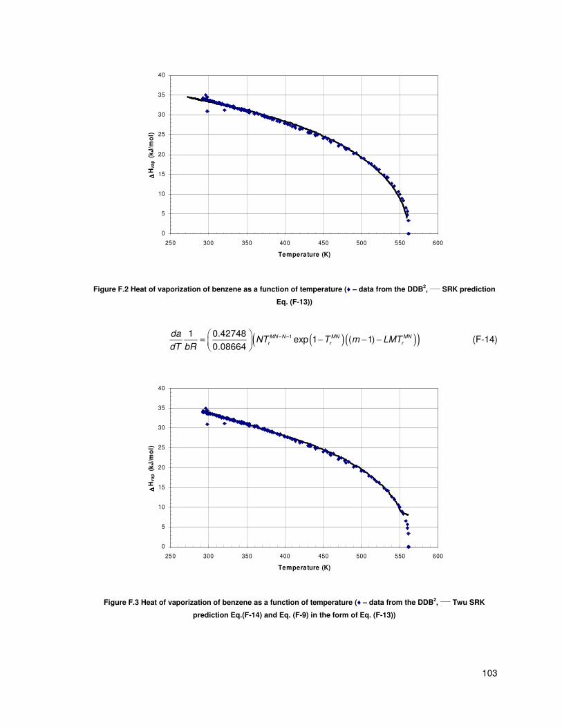
103

0

5

10

15

20

25

30

35

40

250 300 350 400 450 500 550 600

Temperature (K)

∆∆ ∆∆H

va

p (

kJ

/mo

l)

Figure F.2 Heat of vaporization of benzene as a function of temperature (♦ – data from the DDB2,

____ SRK prediction

Eq. (F-13))

( )( )( )11 0.42748exp 1 ( 1)

0.08664

MN N MN MN

r r r

daNT T m LMT

dT bR

− − = − − −

(F-14)

0

5

10

15

20

25

30

35

40

250 300 350 400 450 500 550 600

Temperature (K)

∆∆ ∆∆H

va

p (

kJ

/mo

l)

Figure F.3 Heat of vaporization of benzene as a function of temperature (♦ – data from the DDB2,

____ Twu SRK

prediction Eq.(F-14) and Eq. (F-9) in the form of Eq. (F-13))

104

G CHANGE IN THE CHEMICAL POTENTIAL

Consider the vaporization/condensation of substance A (the +/- ∆ refer to the fact that vaporization

of A is endothermic and condensation of A is exothermic):

( ) ( )l vA A+∆

−∆

→←

The vaporization can be expressed in terms of the change in Gibbs free energy as follows:

v l

A AG µ µ∆ = − (G-1)

The change in Gibbs free energy can also be written in terms equilibrium constant (K):

lnG RT K∆ = − (G-2)

The temperature dependence of the equilibrium constant is given by Eq. (G-3) and is known as the

van’t Hoff equation.

2

lnd K H

dT RT

∆= (G-3)

Therefore for the vaporization of A, ∆H = ∆Hvap and since vaporization is endothermic ∆Hvap will

always be a positive number. This means that an increase of temperature will cause an increase in

the equilibrium constant (Eq. (G-3)) this in turn will cause ∆G to be negative (Eq. (G-2)) which

therefore results in Eq. (2-2).

105

H FURTHER NOTES ON DATA VALIDATION AND DATA USED

As mentioned in paragraph 3.2 the data was validated by plotting the data on the inverse

temperature log pressure axes and removing any outliers. The main reason why such a method

was chosen is that it provides a (relatively) quick method of fairly accurately screening the data.

Unfortunately the problem with this method is that there is no real way to distinguish between good

and poor (this is not to say that the data is very inaccurate but that it is slightly less accurate than

some of the high precision data available in the database) data where there is a slight scatter. [For

examples of this type of scatter see Figure 2.16 and Figure 5.1 – while it is clear that the data is

good there is still a small scatter which is very difficult to rectify]

Data could be screened on the basis of the journal which it comes from, however this may not

always be fair, since experimental errors are not limited to one journal and not another, similarly

with the authors. Another possibility is to produce deviation plots; however this rests on the premise

that there is some basis from which to take the deviation. No doubt for some of the more common

compounds in the database (benzene, hexane etc.) such a basis does exist (e.g. using accurate

Wagner parameters to generate a curve) and could be used fairly successfully, however these

compounds are in the minority and are then subject to external factors (the accuracy of the

parameters). Another approach that was tried was to take the deviation of the data relative to the

line joining the highest and the lowest value. This approach made it very difficult to gauge if the

proper shape of the curve was being maintained. Also for some compounds the endpoints of the

dataset were erroneous which lead to garbage being produced. For this reason the only viable

option which presented itself was to use the 1/T vs. lnP method that was used.

It is for this reason that the errors in section 2.2 may seem a little more inflated that they should be.

For example one would expect the Wagner equation to be able to reproduce the benzene or

hexane curves to within a fraction of a percent. Indeed, which a set of highly accurate data, it can.

However since all the errors reported for this work and the work of Nannoolal were taken relative to

the data that is contained in the database, these same data were used to provide a fairer, more

useful comparison.

Documents

Development of an Improved Group Contribution Method for ... · Development of an Improved Group Contribution Method for the Prediction ... 2.2.3.2 Lee-Kesler method ... using the