Embed Size (px)
Citation preview
Iranian Journal of Oil & Gas Science and Technology, Vol. 2 (2013), No. 3, pp. 11-24
http://ijogst.put.ac.ir
Development of an Intelligent System to Synthesize Petrophysical Well
Logs
M. Nouri Taleghani1, S. Saffarzadeh
2, M. Karimi Khaledi
2, and Gh. Zargar
2*
1 Department of Petroleum Engineering, University of Tehran, Tehran, Iran 2 Department of Petroleum Exploration Engineering, Petroleum University of Technology, Abadan, Iran
Received: May 19, 2013; revised: July 27, 2013; accepted: August 31, 2013
Abstract
Porosity is one of the fundamental petrophysical properties that should be evaluated for hydrocarbon
bearing reservoirs. It is a vital factor in precise understanding of reservoir quality in a hydrocarbon
field. Log data are exceedingly crucial information in petroleum industries, for many of hydrocarbon
parameters are obtained by virtue of petrophysical data. There are three main petrophysical logging
tools for the determination of porosity, namely neutron, density, and sonic well logs. Porosity can be
determined by the use of each of these tools; however, a precise analysis requires a complete set of
these tools. Log sets are commonly either incomplete or unreliable for many reasons (i.e. incomplete
logging, measurement errors, and loss of data owing to unsuitable data storage). To overcome this
drawback, in this study several intelligent systems such as fuzzy logic (FL), neural network (NN), and
support vector machine are used to predict synthesized petrophysical logs including neutron, density,
and sonic. To accomplish this, the petrophysical well logs data were collected from a real reservoir in
one of Iran southwest oil fields. The corresponding correlation was obtained through the comparison
of synthesized log values with real log values. The results showed that all intelligent systems were
capable of synthesizing petrophysical well logs, but SVM had better accuracy and could be used as
the most reliable method compared to the other techniques.
Keywords: Fuzzy logic, Artificial Neural Network, Support Vector Machine, Porosity log, Mean
Square Error
1. Introduction
One of the far-reaching issues in reservoir evaluation is the prediction of petrophysical parameters
such as porosity, lithology, shale volume, formation water saturation, fluid contacts, and productive
zones. These parameters are acquired from well logs. It is quite conventional for several wells in a
field to have incomplete suites of wire-line logs. This is mainly because a full suite of logs is not
obtained at the time the well is logged or because of the problems encountered in repeated logging
such as damaged faulty logging instruments or poor logging conditions in any of the logging runs. In
recent years, intelligent systems have been deemed as powerful tools for modeling and prediction in
the petroleum industry. For example, Lim (2003, 2005), Huang et al. (2001), Mohaghegh (2000),
Cuddy (1998), Soto et al. (1997), Wong et al. (1997) and numerous researchers have applied
intelligent systems to estimate several reservoir parameters from well log responses. The
incorporation of intelligent systems including fuzzy logic (FL), artificial neural networks (ANN), and
* Corresponding Author:
Email: [email protected]

12 Iranian Journal of Oil & Gas Science and Technology, Vol. 2 (2013), No. 3
support vector machine (SVM) into the synthesis of petrophysical well log data is investigated in this
study and the results of the various models are compared with a view to distinguishing the best
intelligent system for solving problems with different methodologies.
2. Methods
2.1. Fuzzy logic (FL)
A fuzzy inference system (FIS) is a procedure of formulation which utilizes a set of input data to a set
of output data by dint of fuzzy sets theory (Matlab user's guide, 2009). Fuzzy logic theory is an
extension of Boolean logic (0, 1), which permits the use of “partial truth” between “entirely true” and
“entirely false” alternatives and reflects the full range of choices between these alternatives (Zadeh,
1965). Each fuzzy set is signified by a membership function (MF). MF’s are of various types such as
Gaussian, triangular, trapezoidal, sigmoid, S-shape, Z-shape, etc. The procedure for fuzzy inference
systems includes the fuzzification of the input variables, the formulation of the fuzzy “if-then” rule-
base, the expansion of the fuzzy inference (i.e. the application of the fuzzy rules), and non-
fuzzification. Among different types of FIS’s, Sugeno fuzzy inference system was employed in this
study. Sugeno and Yasukawa (1993) introduced an FIS in which output membership functions were
constant or linear and were created through the use of a fuzzy clustering process.
2.2. Artificial neural network
Artificial neural network has been defined as a computer model which attempts to mimic simple
biological learning processes and simulate specific functions of human nervous system (Wong et al.,
1997). It has also been referred to as an adaptive parallel information processing system, which is
capable of developing associations, transformations, or mappings between objects or data. It is
expected that ANN will succeed in solving complex problems because it utilizes similar methods used
by millions of neurons in the brain to solve everyday problems. The neurons work together in parallel
to solve tiny bits of a big problem. This type of problem-solving method has shown great capability in
pattern recognition. ANN is also capable of learning in order to recognize, classify, and generalize.
Figure 1 shows the schematic diagram of an artificial neural network.
Figure 1
Schematic diagram of a neural network with one hidden layer

M. Nouri Taleghani et al. / Development of an Intelligent System to Synthesize … 13
2.3. Support vector machine (SVM)
Support vector machines (SVM’s) are a set of related supervised learning methods used for
classification and regression (Gunn, 1998). The most common application form of SVM’s is support
vector regression (SVR). In the SVR method, learning the n-dimensional function based on the data is
the most crucial step. This technique is used for the modeling and analysis of numerical data
consisting of values of a dependent variable and an independent variable. The model is a function of
the independent variables and one or more parameters.
SVR is performed primarily by nonlinearly mapping the input space into a high dimensional feature
space and then running the linear regression in the output space. Thus linear regression in the output
space corresponds to nonlinear regression in the low dimensional input space.
Consider a training data set��x�, �y��}��, where xϵR� is the input space. The SVR developed by
Vapnikrelies for estimating a linear regression function can be given by (Equation 1):
f�x� = ⟨w, �x⟩� + b (1)
where, w and b is the slope and offset of the regression line respectively; ⟨. , �. ⟩� denotes the dot product
in X. Flatness in above means that one seeks a small w (Smola and Schölkopf, 2003). A way to ensure
this is to minimize the norm, i.e. ‖w‖� = ⟨w, �w⟩�. Writing this problem as a convex optimization
problem, one may obtain:
minimize�� || w ||2
subject to:
�y� − ⟨w, �x�⟩� − b ≤ ε⟨w, �x�⟩� + b − y ≤ ε � (2)
As mentioned above, the regression function is calculated by minimizing the objective function and it
is subjected to the corresponding constraints:
Minimize
�� ‖w‖� + c∑ �ξ�, ξ�∗�!�"� (3)
subject to
# y�⟨w. �x�⟩ − b ≤ ε + ξ� �⟨w, �x�⟩� + b − y� ≤ ε + ξ�$% , $%∗ ≥ 0 � (4)
where, �� ‖w‖ is the term characterizing the model complexity (the smoothness of f(x)) and c∑ �$% , $%∗�!�"� is the loss function determining how the distance between f(xi) and the target values yi
should be penalized. The slack variables $% and $%∗are introduced for the situation that the target value
exceeds more than ε (see Figure 2). The constant C>0 determines the trade-off between the flatness of
f (model complexity) and the amount to which deviations larger than ε are tolerated (empirical error).
The commonly used ε -insensitive loss function was introduced by Vapnik. This ε-insensitive loss
function |ξ|ε is defined by:
|ξ|) = � 0if|ξ| ≤ ε|ξ| − εotherwise� (5)

14 Iranian Journal of Oil & Gas Science and Technology, Vol. 2 (2013), No. 3
In fact, this particular constraint defines a tube with radius ε around the hypothetical regression
function in such a way that if a data point is positioned in this tube, the loss function equals 0, while if
a data point lies outside the tube, the loss is proportional to the magnitude of the Euclidean difference
between the data point and the radius ε of the tube. The points lying outside the ε tube are named
support vectors (SV’s), because they will be used to estimate regression function. This implies that all
other data points are in fact not important for inclusion into the model and can be removed after the
SVR model has been constructed. Hence usually (much) fewer training points do constitute the
regression model.
Figure 2
The soft margin loss setting for a linear SVM
Graphically, this condition is shown in Figure 2; only the points outside the shaded region contribute
to the cost insofar as the deviations are penalized in a linear fashion. If one intended to extend the
SVM linear case to nonlinear functions, the standard dualization method using Lagrangian multipliers
is necessitated.
A nonlinear generalization is affected by the fact that the resulting solution f(x) can be explicitly
written in terms of inner products between data points; these inner products are then replaced by a
Mercer kernel k�x, �x��� and the resulting solution has the form of:
f�x� = ∑ �a� − a�∗�k�x, �x�� + b��!�"� (6)
a. Kernel functions
In the non-linear problems, input data are mapped into a higher-dimensional feature space to increase
the computational power of the linear-learning machine to solve nonlinear problems. Kernel
representations project the data; thus the nonlinear regression function in an input space is constructed
by considering a linear-regression hyperplane in the feature space. Therefore, to create a nonlinear
regression function, the input vectors x are mapped into vectors of a higher-dimensional feature space,
and then a linear-regression problem is solved in this feature space. In the example shown in Figure 3,
a separator can easily classify the data into higher dimensions (Manning et al., 2008). Mercer’s
theorem is used to perform this operation. It states that any continuous, symmetric, positive semi-
definite kernel function k(x,y) can be expressed as a dot product in a high-dimensional space. The
kernel transformation transforms any algorithm that solely depends on the dot product between two
vectors. In other words, wherever a dot product is used, it is replaced with a kernel function. The most
ζ
ζ*
+ε
-ε 0
bxy += ω
∑=
++N
i
iiC1
*2)(
2
1ζζω
0, *
*
≥
+≤−+
+≤−−
ii
iii
iii
ybx
bxy
ζζ
ζεω
ζεω

M. Nouri Taleghani et al. / Development of an Intelligent System to Synthesize … 15
common kernel functions can be summarized as given in Table 1 (Cristianini and Shawe-Taylor,
2000).
Figure 3
Classification of the data into higher dimensions
Table1
Common forms of kernel functions
Type of kernel Form
Linear 2�3% , 3� = ⟨3% , 3⟩ Gaussian Radial Basis Function 2�3% , 3� = 456786599:9
Sigmoid 2�3% , 3� = ;<=ℎ?2�3% , 3� + @A 3. Case study
The data set for this study is obtained from a real reservoir in one of Iran southwest oil fields. A total
of 1328 data points are used to construct the models. In order to have accurate prediction, the log
information of three wells No. z1, No. z2, and No. z3 is used. The well No. z1 has a total of 623 data
points; the well No. z2 has 226 data and the well No. z3 includes a total number of 479 data points.
The fullest logs consist of the log plots of gamma ray log (GR), bulk density log (RHOB), neutron log
(NPHI), resistivity log (RT), and sonic travel time log (DT). The appropriate input data for predicting
NPHI, DT, and RHOB are selected by quick look correction coefficients. Appropriate inputs to
construct intelligent models are shown in Table 2. As mentioned before, the models are performed
using three different intelligent systems, namely fuzzy logic, ANN, and SVM.
16 Iranian Journal of Oil & Gas Science and Technology, Vol. 2 (2013), No. 3
Table2
Appropriate inputs to construct intelligent models
Predicted well log NPHI RHOB DT
Inputs RHOB, DT, and GR NPHI and DT NPHI, RHOB, and GR
3.1. Fuzzy logic
a. Sugeno FIS (SFIS)
In this work, a TSK-FIS was implemented for the prediction of porosity log (RHOB, NPHI, and DT)
in Matlab. All input and output membership functions (MF’s) and their corresponding parameters
were attained by dint of a subtractive clustering method and then a set of fuzzy “if-then” rules were
developed. Subtractive clustering is an operative procedure for the estimation of the number of fuzzy
clusters and cluster centers in a Sugeno fuzzy inference system (Jarrah and Halawani, 2001). In
subtractive clustering, each data point is considered as a potential cluster center. Furthermore, in
subtractive clustering, when the influence range or cluster radius (Ra) is varied, the number of the
MF’s and “if-then” rules changes as well (Anifowose and Abdulraheem, 2011). A small cluster radius
usually yields more MF’s and “if-then” rules, whereas a large cluster radius results in fewer MF’s and
“if-then” rules (Chiu, 1997). With the view to obtaining an optimal number of rules and MF’s, a set of
values for the clustering radius was specified which ranged from 0 to 1. Consequently, several
numbers of rules were generated and the MSE for each of these models was measured. The model
with highest performance (lowest error) was selected as the optimum FIS (Table 3).
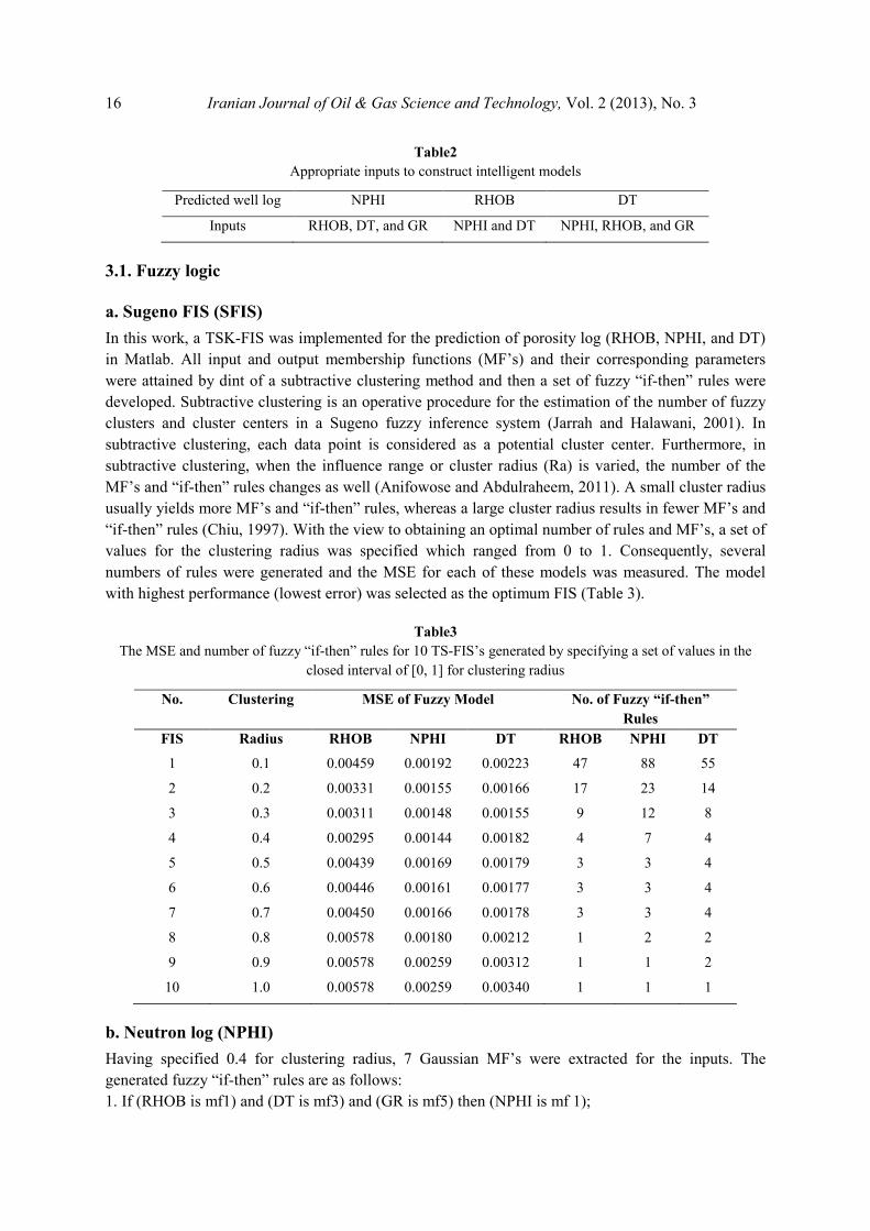
Table3
The MSE and number of fuzzy “if-then” rules for 10 TS-FIS’s generated by specifying a set of values in the
closed interval of [0, 1] for clustering radius
No. Clustering MSE of Fuzzy Model No. of Fuzzy “if-then”
Rules
FIS Radius RHOB NPHI DT RHOB NPHI DT
1 0.1 0.00459 0.00192 0.00223 47 88 55
2 0.2 0.00331 0.00155 0.00166 17 23 14
3 0.3 0.00311 0.00148 0.00155 9 12 8
4 0.4 0.00295 0.00144 0.00182 4 7 4
5 0.5 0.00439 0.00169 0.00179 3 3 4
6 0.6 0.00446 0.00161 0.00177 3 3 4
7 0.7 0.00450 0.00166 0.00178 3 3 4
8 0.8 0.00578 0.00180 0.00212 1 2 2
9 0.9 0.00578 0.00259 0.00312 1 1 2
10 1.0 0.00578 0.00259 0.00340 1 1 1
b. Neutron log (NPHI)
Having specified 0.4 for clustering radius, 7 Gaussian MF’s were extracted for the inputs. The
generated fuzzy “if-then” rules are as follows:
1. If (RHOB is mf1) and (DT is mf3) and (GR is mf5) then (NPHI is mf 1);

M. Nouri Taleghani et al. / Development of an Intelligent System to Synthesize … 17
2. If (RHOB is mf6) and (DT is mf2) and (GR is mf7) then (NPHI is mf 1);
3. If (RHOB is mf3) and (DT is mf4) and (GR is mf4) then (NPHI is mf 1);
4. If (RHOB is mf5) and (DT is mf6) and (GR is mf2) then (NPHI is mf 1);
5. If (RHOB is mf7) and (DT is mf1) and (GR is mf3) then (NPHI is mf 1);
6. If (RHOB is mf2) and (DT is mf5) and (GR is mf6) then (NPHI is mf 1);
7. If (RHOB is mf1) and (DT is mf7) and (GR is mf1) then (NPHI is mf 1).
c. Sonic log (DT)
By specifying 0.3 for clustering radius, 8 Gaussian MF’s were extracted for the inputs. The generated
fuzzy “if-then” rules are as follows:
1. If (NPHI is mf3) and (RHOB is mf3) and (GR is mf2) then (DT is mf7);
2. If (NPHI is mf1) and (RHOB is mf6) and (GR is mf5) then (DT is mf4);
3. If (NPHI is mf5) and (RHOB is mf2) and (GR is mf3) then (DT is mf5);
4. If (NPHI is mf6) and (RHOB is mf5) and (GR is mf8) then (DT is mf6);
5. If (NPHI is mf4) and (RHOB is mf7) and (GR is mf4) then (DT is mf3);
6. If (NPHI is mf8) and (RHOB is mf1) and (GR is mf1) then (DT is mf2);
7. If (NPHI is mf7) and (RHOB is mf4) and (GR is mf7) then (DT is mf8);
8. If (NPHI is mf2) and (RHOB is mf8) and (GR is mf6) then (DT is mf1).
d. Density log (RHOB)
By specifying 0.4 for clustering radius, 4 Gaussian MF’s were extracted for the inputs. The generated
fuzzy “if-then” rules are as follows:
1. If (NPHI is mf2) and (DT is mf2) then (RHOB is mf1);
2. If (NPHI is mf1) and (DT is mf1) then (RHOB is mf2);
3. If (NPHI is mf3) and (DT is mf3) then (RHOB is mf3);
4. If (NPHI is mf4) and (DT is mf4) then (RHOB is mf4).
For example, Figure 4 shows the TSK-FIS Gaussian membership functions extracted for the
prediction of RHOB. Subsequent to the preparation of the fuzzy models, the input matrix of test data
was input to the SFIS models. The measured mean squared error (MSE) functions for the FL-
predicted NPHI, DT, and RHOB in the test data were equal to 0.00145, 0.00156, and 0.00296
respectively. The R2 between the measured and FL-predicted NPHI, DT, and RHOB were 0.89 and
0.87, and 0.91 respectively (Figure 5). For example, a contrast between the measured and FL-
predicted outputs versus depth of the test data is shown in Figure 6.

18 Iranian Journal of Oil & Gas Science and Technology, Vol. 2 (2013), No. 3
Figure 4
Membership functions for RHOB modeling by Sugeno FIS
Figure 5
Crossplots showing the correlation coefficients between actual and predicted results using FL for NPHI, DT,
and RHOB
R² = 0.87
80
85
90
95
100
105
110
80 100 120
DT
fro
m F
L(µ
s/ft
)
Actual DT(µs/ft)
R² = 0.899
0.2
0.25
0.3
0.35
0.4
0.45
0.5
0.2 0.4 0.6
NP
HI
fro
m F
L (
v/v
)
Actual NPHI(v/v)
R² = 0.91
2.3
2.4
2.5
2.6
2.7
2.8
2.9
2.2 2.4 2.6 2.8 3
RH
OB
fro
m F
L(g
/cm
3)
Actual RHOB(g/cm3)
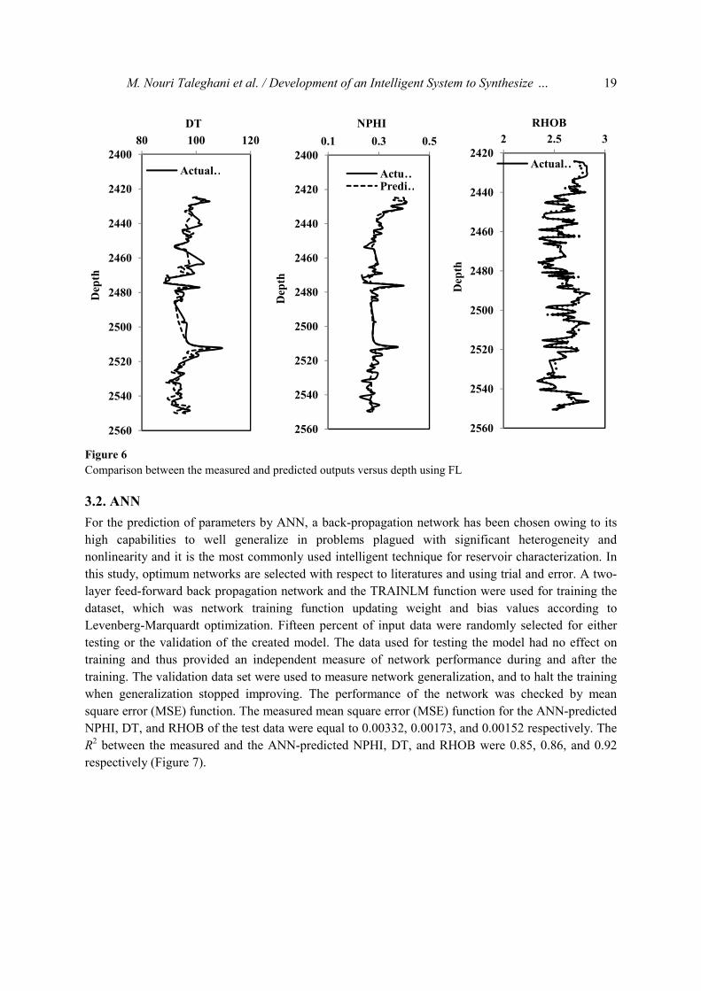
M. Nouri Taleghani et al. / Development of an Intelligent System to Synthesize … 19
Figure 6
Comparison between the measured and predicted outputs versus depth using FL
3.2. ANN
For the prediction of parameters by ANN, a back-propagation network has been chosen owing to its
high capabilities to well generalize in problems plagued with significant heterogeneity and
nonlinearity and it is the most commonly used intelligent technique for reservoir characterization. In
this study, optimum networks are selected with respect to literatures and using trial and error. A two-
layer feed-forward back propagation network and the TRAINLM function were used for training the
dataset, which was network training function updating weight and bias values according to
Levenberg-Marquardt optimization. Fifteen percent of input data were randomly selected for either
testing or the validation of the created model. The data used for testing the model had no effect on
training and thus provided an independent measure of network performance during and after the
training. The validation data set were used to measure network generalization, and to halt the training
when generalization stopped improving. The performance of the network was checked by mean
square error (MSE) function. The measured mean square error (MSE) function for the ANN-predicted
NPHI, DT, and RHOB of the test data were equal to 0.00332, 0.00173, and 0.00152 respectively. The
R2 between the measured and the ANN-predicted NPHI, DT, and RHOB were 0.85, 0.86, and 0.92
respectively (Figure 7).
2400
2420
2440
2460
2480
2500
2520
2540
2560
80 100 120
Dep
th
DT
Actual …
2400
2420
2440
2460
2480
2500
2520
2540
2560
0.1 0.3 0.5
Dep
th
NPHI
Actu…Predi…
2420
2440
2460
2480
2500
2520
2540
2560
2 2.5 3
Dep
th
RHOB
Actual …

20 Iranian Journal of Oil & Gas Science and Technology, Vol. 2 (2013), No. 3
Figure 7
Crossplots showing the correlation coefficients between the actual and predicted results using ANN for NPHI,
DT, and RHOB
3.3. SVM
Generally, the SVM model includes two phases, namely training and testing; hence the data should be
divided into two parts. Conventionally, the training data set is larger than the testing data set; thus
wells No. z1 and No. z3 were selected as the training wells and well No. z3 as the testing data well.
Then, the training data set was submitted to each regression algorithm to construct the model. The
DTREG (Sherrod, 2009) software package was used to generate the prediction models. The
parameters of both SVR-model and kernel-function were selected by using grid and pattern search.
This software provides two methods for finding optimal parameter values, namely a grid search and a
pattern search. A grid search tries values of each parameter across the specified search range using
geometric steps, while a pattern search starts at the middle of the search range and creates trial steps in
each direction for each parameter. If the fit of the model improves, the search center moves to the new
point and the process is repeated. However, if no improvement is achieved, the step size is reduced
and the search procedure is executed again. The pattern search stops when the search step size is
reduced to a specified tolerance. Cross-validation is used to avoid over fitting. For SVR, models with
linear, sigmoid, and Gaussian RBF kernel functions were constructed to compare their accuracy and
strength in data prediction. In this work, the Epsilon-SVR and Nu-SVR machine techniques were
used. The trade-off parameters in the SVM regression scheme were based on the recommended
defaults. The measured mean square error (MSE) function for the SVM-predicted NPHI, DT, and
RHOB of the test data were equal to 0.00315, 0.00082, and 0.00116 respectively. The R2 between the
R² = 0.92
2.2
2.3
2.4
2.5
2.6
2.7
2.8
2.9
2.2 2.4 2.6 2.8 3
RH
OB
fro
m S
VM
(g/c
m3)
Actual RHOB(g/cm3)
R² = 0.85
0.2
0.25
0.3
0.35
0.4
0.45
0.5
0.2 0.4 0.6
NP
HI
from
AN
N(v
/v)
Actual NPHI(v/v)
R² = 0.86
80
85
90
95
100
105
110
80 90 100 110
DT
fro
m A
NN
(µs/
ft)
Actual DT(µs/ft)

M. Nouri Taleghani et al. / Development of an Intelligent System to Synthesize … 21
measured and SVM-predicted NPHI, DT, and RHOB were 0.86, 0.96, and 0.94 respectively (Figure
8).
Figure 8
Crossplots showing the correlation coefficients between the actual and predicted results using SVM for NPHI,
DT, and RHOB
4. Results and discussion
The ultimate test for any technique that bears the claim of reservoir rock parameter prediction is the
accuracy and verifiability of the prediction using well log and laboratory experiments. In this study,
several intelligent systems like fuzzy logic (FL), neural network (NN), and support vector machine
are used to predict the synthesized petrophysical logs.
Table 4 depicts the comparisons of error statistics for the test data using different intelligent systems.
The MSE achieved by these intelligent systems are in proximity to each other and it could be
concluded that all of such techniques could exclusively be a powerful tool for the estimation of NPHI,
DT, and RHOB.
The comparisons between the measured and predicted parameters using different methods indicated
that all the techniques were successful, but SVM could predict better than FL and ANN; however,
some exceptions were on hand. For instance, in well 3, the BPNN appeared to have better
performance than the linear SVR. From Table 5, the BPNN model is less accurate as compared to the
SVM. This is mainly due to the techniques used to ensure the generalization capability of the ANN.
Since the wells used in the case study are from a real world reservoir and it is dealing with a lot of
errors, such as the errors in well logging instruments or measuring parameters in laboratory, the
accuracy of the prediction using BPNN depends heavily on the generalization ability of the
R² = 0.94
2.3
2.4
2.5
2.6
2.7
2.8
2.9
2.2 2.7 3.2
RH
OB
fro
m S
VM
(g/c
m3)
Actual RHOB(g/cm3)
R² = 0.86
0.2
0.25
0.3
0.35
0.4
0.45
0.5
0.2 0.4 0.6
NP
HI
from
SV
M(v
/v)
Actual NPHI(v/v)
R² = 0.96
80
85
90
95
100
105
110
115
80 100 120
DT
fro
m S
VM
(µ
s/ft
)
Actual DT(µs/ft)

22 Iranian Journal of Oil & Gas Science and Technology, Vol. 2 (2013), No. 3
determination model. It is confirmed that SVM could be an appropriate alternative intelligent
technique for reservoir characterization.
Table 4
Comparisons of MSE for (a) NPHI, (b) DT, and (c) RHOB of the test data using different intelligent systems
(a)
Intelligent Systems MSE Rank
TKS-F1S 0.00296 1
ANN 0.00332 3
SVM 0.00315 2
(b) Intelligent Systems MSE Rank
TKS-F1S 0.00145 2
ANN 0.00173 3
SVM 0.00082 1
(c)
Intelligent Systems MSE Rank
TKS-F1S 0.00156 3
ANN 0.00152 2
SVM 0.00116 1
Table 5
Comparison of correlation coefficients of SVR, ANN, and FL methods
ANN FL SVR Kernel Function
Linear Sigmoid RBF
NPHI 0.844 0.886 0.84 0.86 0.85
DT 0.845 0.866 0.87 0.96 0.91
RHOB 0.915 0.903 0.91 0.94 0.92
5. Conclusions
Intelligent systems are quick, robust, and convenient to use for the prediction of well logs and solving
complicated problems compared with conventional methods which impose more difficulties, time
consumption, and high expenses. The results show that ANN, FL, and SVM can successfully be used
in the quantitative formulation of well log responses in one of Iran southwest oil fields. This study
indicated that intelligent synthesizing of petrophysical well logs by the use of other well logs data is a
highly feasible method. Both synthesized and real petrophysical well logs were presented to
demonstrate that well logs were synthesized with a high degree of accuracy. The comparisons among
the measured and predicted parameters using different methods showed that all the methods had
similarities, but SVM could predict better than the others. Accordingly, the SVM technique was
expected to provide more accurate and suitable results in other wells. This models constructed by
SVM approach could be extended to other intervals and wells. The developed models did not
incorporate depth or lithological as a part of the input parameters, meaning the utilized methodology
was applicable to any field.

M. Nouri Taleghani et al. / Development of an Intelligent System to Synthesize … 23
Nomenclature
FL : Fuzzy logic
ANN : Artificial neural network
SVM : Support vector machine
BP-ANN : Back propagation artificial neural network
DT : Sonic transit time log (µs/ft)
GR : Gamma ray log (API)
NPHI : Neutron log (v/v)
RHOB : Density log (gr/cm3) $, $∗ : Slake variables σ : Variance σ� : Standard deviation
x : Input parameter
y : Output variable yC : Estimated output value a,a∗ : Lagrangian multiplier to be determined ε : Error accuracy
References
Anifowose, F. and Abdulraheem, A., Fuzzy Logic-driven and SVM-driven Hybrid Computational
Intelligence Models Applied to Oil and Gas Reservoir Characterization, Journal of Natural Gas
Science and Engineering, Vol. 3, p. 505-517, 2011.
Chiu, S., Extracting Fuzzy Rules from Data for Function Approximation and Pattern Classification, in
Dubois, D., Prade, H., Yager, R. (Eds.), Fuzzy Information Engineering: A Guided Tour of
Applications, John Wiley & Sons, New York, p. 149-162, 1997.
Cristianini, N. and Shaw-Taylor, J., An Introduction to Support Vector Machines and Other Kernel-
based Learning Methods, New York, Cambridge University Press, 189 p, 2000.
Cuddy, S. J., Litho-facies and Permeability Prediction from Electrical Logs Using Fuzzy Logic, 8th
Abu Dhabi International Petroleum Exhibition and Conf., SPE 49470, November, 1998.
Gunn, S. R., Support Vector Machines for Classification and Regression, Technical Report, Dept. of
Electronics and Computer Science, University of Southampton, Southampton, U.K., 54 p, 1998.
Huang Y., Gedeon, T. D., and Wong P. M., An Integrated Neural-fuzzy-genetic-algorithm Using
Hyper-surface Membership Functions to Predict Permeability in Petroleum Reservoirs, J. Eng.
Appl. Artif. Intell, Vol. 14, p. 15-21, 2001.
Jarrah, O. A. and Halawani, A., Recognition of Gestures in Arabic Sign Language Using Neuro-fuzzy
Systems, Artificial Intelligence Vol. 133, p. 117-138, 2001.
Kadkhodaie-Ilkhchi, A., Rahimpour-Bonab, H., and Rezaee, M. R., A Committee Machine with
Intelligent Systems for Estimation of Total Organic Carbon Content from Petrophysical Data:
An example from Kangan and Dalan Reservoirs in South Pars Gas Field, Iran., J. Comput.
Geosci., Vol. 35, p. 459-474, 2008.
Lim, JongSe., Reservoir Properties Determination Using fuzzy Logic and Neural Networks from Well
Data in Offshore Korea, Journal of Petroleum Science and Engineering, Vol. 49, p. 182-192,
2005.
Manning, C. D., Raghavan, P., and Schutze, H., Introduction to Information Retrieval, Cambridge
University Press, 2008.
Matlab User's Guide, Fuzzy Logic, Direct Search Toolboxes, Matlab CD-ROM, by the Math Works,
Inc., 2009.

24 Iranian Journal of Oil & Gas Science and Technology, Vol. 2 (2013), No. 3
Mohaghegh, S., Virtual-intelligence Applications in Petroleum Engineering: Part I., Artificial Neural
Networks J. Pet. Technol., Vol. 52, p. 64-73, 2000.
Schölkopf, B. and Smola, A. J., Learning with Kernels: Support Vector Machines, Regularization,
Optimization, and Beyond, Cambridge, MIT Press, 2002.
Smola, A. J., and Schölkopf, B., A Tutorial on Support Vector Regression, Statistics and Computing,
Vol. 14, No. 3, p. 199-222, 2004.
Soto, B. R., Ardila, J. F., Ferneynes, H., and Bejarano A., Use of Neural Networks to Predict the
Permeability and Porosity of Zone “C” of the Cantagallo Field in Colombia Proc., SPE
Petroleum Computer Conf. (Dallas, TX) SPE 38134, June, 1997.
Sugeno, M., Yasukawa, T., A Fuzzy-logic-based Approach to Qualitative Modeling. IEEE Trans.
Syst. Man Cybern., Vol. 1, p. 201-224, 1993.
Wong, P. M., Henderson, D. J., and Brooks, L. J., Reservoir Permeability Determination from Well
Log Data Using Artificial Neural Networks: An Example from the Ravva Field, Offshore India,
SPE Paper 38034, April, 1988.
Zadeh, L. A., Fuzzy Sets, Information and Control, Vol. 8, p. 338-353, 1997.