DEVELOPMENT OF METHODOLOGY FOR DESIGNING WAVE DISK …

DEVELOPMENT OF METHODOLOGY FOR DESIGNING WAVE DISK ENGINE BASED

ON WAVE DYNAMICS AND THERMODYNAMIC ANALYSIS

By

Dewashish Prashad

A THESIS

Submitted to

Michigan State University

in partial fulfillment of the requirements

for the degree of

Mechanical Engineering--Master of Science

2014

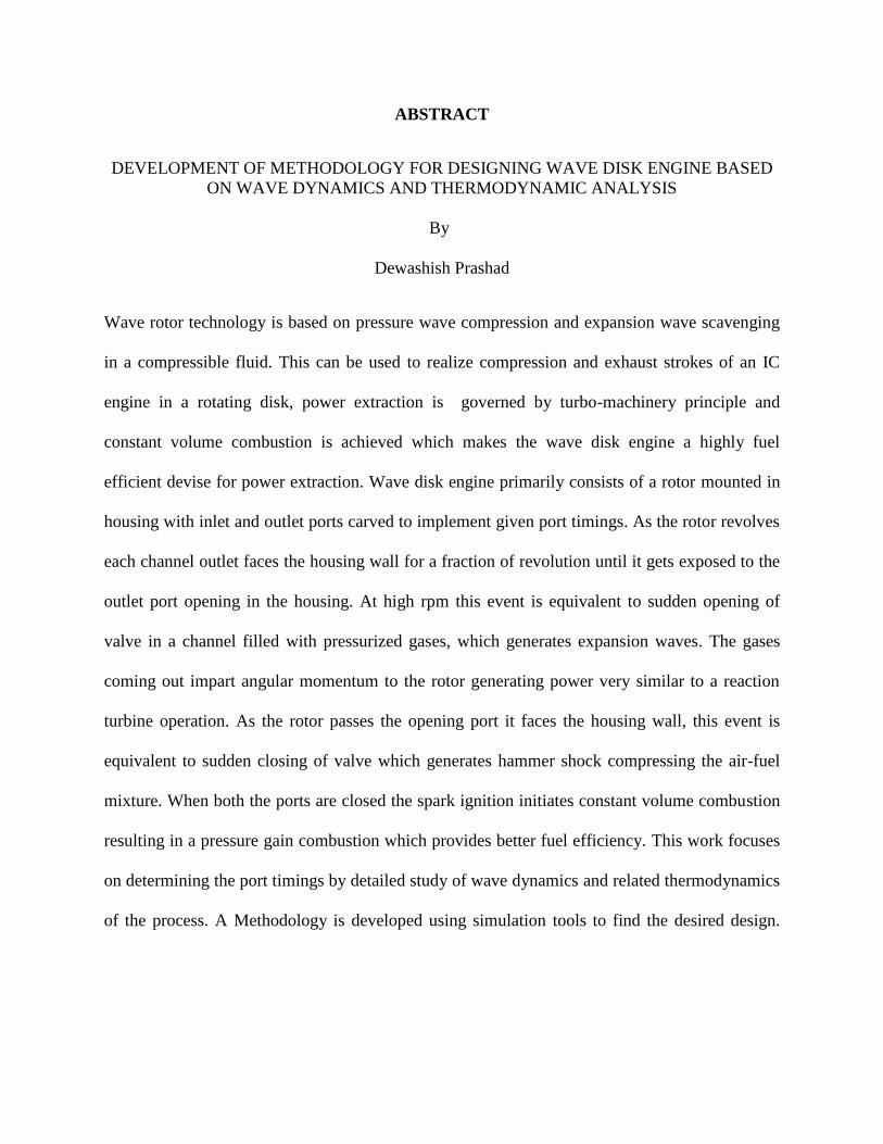
ABSTRACT

DEVELOPMENT OF METHODOLOGY FOR DESIGNING WAVE DISK ENGINE BASED

ON WAVE DYNAMICS AND THERMODYNAMIC ANALYSIS

By

Dewashish Prashad

Wave rotor technology is based on pressure wave compression and expansion wave scavenging

in a compressible fluid. This can be used to realize compression and exhaust strokes of an IC

engine in a rotating disk, power extraction is governed by turbo-machinery principle and

constant volume combustion is achieved which makes the wave disk engine a highly fuel

efficient devise for power extraction. Wave disk engine primarily consists of a rotor mounted in

housing with inlet and outlet ports carved to implement given port timings. As the rotor revolves

each channel outlet faces the housing wall for a fraction of revolution until it gets exposed to the

outlet port opening in the housing. At high rpm this event is equivalent to sudden opening of

valve in a channel filled with pressurized gases, which generates expansion waves. The gases

coming out impart angular momentum to the rotor generating power very similar to a reaction

turbine operation. As the rotor passes the opening port it faces the housing wall, this event is

equivalent to sudden closing of valve which generates hammer shock compressing the air-fuel

mixture. When both the ports are closed the spark ignition initiates constant volume combustion

resulting in a pressure gain combustion which provides better fuel efficiency. This work focuses

on determining the port timings by detailed study of wave dynamics and related thermodynamics

of the process. A Methodology is developed using simulation tools to find the desired design.

iii

This work is dedicated to my dear parents: Mr Kanta Prasad and Mrs. Roopwati Prasad, my

lovely brothers Rohit and Shailesh and all wonderful friends who has supported me throughout

the two years of my hard work in achieving this milestone

iv

ACKNOWLEDGEMENTS

I would like to thank Dr. Norbert Mueller, my thesis adviser for his support and inspiration,

without his guidance this work wouldn’t be possible. Also I want to thank all my peers who

worked with me on the wave disk project, there inputs have been critical in every analysis done

in this study. I am specially thankful to Dr. Rohitashwa Kiran, my fellow project-mate, who

mentored me throughout my study on wave disk engine. Also I want to thank my family and

friends (Abhisek Jain, Itishree Swain, Nanda Kumar Sasi, Jessica Mesaros and Anju Kurian)

who has given there constant support throughout the period of my Master’s degree.

v

TABLE OF CONTENTS

LIST OF TABLES vii

LIST OF FIGURES ix

KEY TO SYMBOLS AND ABBREVIATIONS xii

CHAPTER 1 Introduction

CHAPTER 2 Straight Channel Analysis 4

2.1 Straight Channel 6

2.2 Comparison of different channel shapes 11

2.3 Discussion

CHAPTER 3 Analysis of curved rotor shapes 14

3.1 Analysis of Rotor A 14

3.1.a) Simulation of Design A of rotor 16

3.1.b) Post Processing of the simulation results 21

3.1.c) Port Timing Calculation 25

3.2 Analysis of Rotor B 28

3.2.a) Similar Methodology is applied to this rotor – simulation results 29

3.2.b) Simulations for Rotor B with prescribed ω 33

3.3 Analysis of rotor C 36

3.3.a) Chronological Summary of Simulation 39

3.4 Comparison of Rotor A, B and C 41

3.4.a) Discussion 43

3.5 Modified Rotor A 45

3.5.a) Simulation Summary 47

3.5.b) Chronological Summary of Simulation 49

3.5.c) Comparison of Rotor A vs Modified Rotor A 51

CHAPTER 4 Conclusion and Future Work 52

REFERENCES 53

vi

LIST OF TABLES

Table 1 Quantitative results for the cycle 25

Table 2 RPM 26

Table 3 Time History of the Cycle 26

Table 4 Angular History of the Cycle 26

Table 5 Cycle Summary from Simulations 31


Table 7 RPM 32





Table 12 RPM 34




vii


Table 17 RPM 40

Table 18 Time History of the Cycle a 40


Table 20 Comparison of the three rotors 41



Table 23 RPM 50



viii

LIST OF FIGURES

Figure 0: Schematic for Wave disc Engine 1

Figure 1: Sample image depicting simulation initialization 5

Figure 2: Schematic of Straight Channel at 7 bar pressure

(graph depicts pressure distribution in the channel) 6

Figure 3: Representation of the Cycle 8

Figure 4: Diverging Straight Channel 9

Figure 5: Converging Straight Channel 10

Figure 6: P-v diagram and T-s diagram 11

Figure 7: P-v diagram for straight, diverging and converging channel shape 12

Figure 8: Rotor of WDE, the right side of the figure represent top view. 14

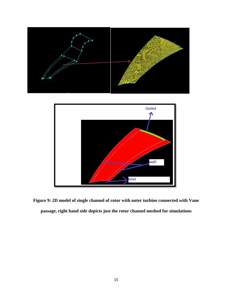
Figure 9: 2D model of single channel of rotor with outer turbine connected

with Vane passage, right hand side depicts just the rotor channel

meshed for simulations 15

Figure 10: Simulation Initialization 16

Figure 11: EVO : Burnt mixture is rushed out (time =0 ) 18

Figure 12: Intermidiate Step of the EVO mode (time =.05ms) 18

Figure 13: The pressure at inlet falls below atmospheric pressure,

the inlet port is opened now: IVO (time =.164 ms) 19

ix

Figure 14: The air-fuel mixture is sucked into the channel,

the pressure inside the channel rises up slightly (time = .193 ms) 19

Figure 15: The outlet port is closed : EVC (time = .455 ms) 20

Figure 16: The Shockwave reaches the inlet port resulting in precompression

(time=.650 ms) 20

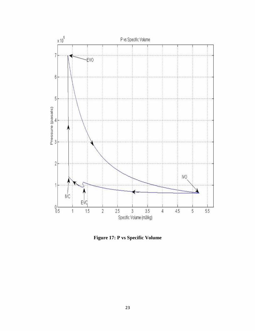
Figure 17: P vs Specific Volume 23

Figure 18: Torque History 24

Figure 19: Depiction of Inlet and Outlet angles 27

Figure 20: 3D view for Rotor B 28

Figure 21: 2D Projection for a rotor channel 28

Figure 22: Sample image durung intermediate time step after exhaust port is opened 29

Figure 23: P-v diagram and the Torque History 30

Figure 24: Sample image right before exhaust port is opened 36

Figure 25: P-v and T-s Diagram 37


Figure 27: Comparison of Rotor A, B and C 41

Figure 28: Comparison of P-v diagram 42

Figure 29: Torque-History of all three rotors 43

Figure 30: Mass-flow-rate at the outlet of the rotors. 44

x

Figure 31: 3D view of Rotor A- with external row of turbine 45

Figure 32: Modified Rotor Channel with external channel 46

Figure 33: Sample image from simulations, depicting pressure

contour after the outlet port is opened 47

Figure 34: P-v ans T-s Diagram 48


Figure 36: Comparitive P-v diagram 51

xi

KEY TO SYMBOLS AND ABBREVATIONS

WDE Wave Disc Engine

EVO Exhaust Valve Open

IVO Inlet Valve Open

EVC Exhaust Valve Closed

L Length of channel

H Height of Channel

P Pressure

V Specific Volume

T Temperature

S Specific entopy

We Work done during expansion

Ws Work done during suction of fuel

Q Heat transfer during one cycle

Η Cycle efficiency

Wc Work done during compression

t1 (EVO) Time period during EVO

t2 (IVO) Time period during IVO

t3 (EVC) Time period during EVC

t4 (IVC) Time period during IVC

T Total Cycle Time

ϴ1 Angle WDE traverse during EVO

xii

ϴ2 Angle WDE traverse during IVO

ϴ3 Angle WDE traverse during EVC

ϴ4 Angle WDE traverse during precompression

step

ϴe Exhaust Angle for WDE

ϴi Inlet Angle of WDE

ω Angular speed of WDE

1

CHAPTER 1

Introduction

Figure 0: Schematic for Wave disc Engine

Wave disk engine is a novel internal combustion engine [2] which stands apart in terms of fuel

efficiency and power to weight ratio in the domain of small scale power output devices. Wave

2

disk engine utilizes work extraction by reaction turbine mechanism via a rotor revolving in a

housing. This is very similar to a gas turbine but the crucial difference is the ability of WDE to

achieve pressure gain combustion [3]. There is no external compressor involved for pre-

compression but the hammer shock waves generated by sudden closing of outlet port provides

pre-compression for the fresh air-fuel mixture.

Cycle starts right after the combustion ends. The gas inside the rotor channel is at very high

pressure and temperature. As the channel revolves to face the exhaust port opening in the stator,

the gases starts to rush out generating expansion waves. During this transient channel emptying

process, there will be a stage where the channel pressure goes below ambient pressure. At this

particular time the inlet port opens up and the fresh air-fuel mixture is sucked in. The gases are

still rushing out at the outlet of rotor channel, the order of velocity magnitude is typically 100-

200 m/s. As the channel revolves to see the wall at the outlet, a hammer shock is generated as a

result of this sudden closing. This compresses the air-fuel mixture. When the compression waves

reaches the inlet port, the inlet port closes (channel revolves to face wall at inlet). At this point

spark is ignited and combustion begins.

This cycle is referred as Humphrey-Cycle for gas turbines and Atkinson’s cycle for IC engine.

When the pre-compression pressure ratio is very low, then the cycle is referred as Lenoir cycle.

The unique features of WDE are its constant volume combustion, compression achieved by

shock waves hence no moving element is required and simple physical design which reduces

manufacturing cost. Although as the pre-compression is not high therefore WDE belongs to

small scale power generation devices.

3

This work investigates design features for WDE by analyzing 3 different proposed designs of

rotors. The heart of design is the estimation of port timing. A methodology is developed to obtain

the port timings using numerical simulations using Ansys Fluent commercial package.

The report begins with basic study of wave propagation in straight channel, then based on the

inferences three proposed designs are analyzed and optimized design is suggested.

4

CHAPTER 2

Straight Channel Analysis

Propagation of waves in gases is widely researched phenomenon [1]. As mentioned before, wave

dynamics critically affects the determination of port timings [7]. To begin with, propagation of

waves in a straight channel is analyzed. Next step would be to investigate effect of change in

area or curvature of the channel on the wave propagation. This understanding will be helpful in

optimizing channel shape to achieve pre-compression and desired scavenging.

Fluent Simulation start-up details:-

Density based solver is used with inviscid flow model. Roe-Fds scheme is used for discretization

with courant number as 1. Explicit formulation for time step is used. Hence the simulation is

primarily a marching method in time.

5

Figure 1: Sample image depicting simulation initialization

6

2.1 Straight Channel

Figure 2: Schematic of Straight Channel at 7 bar pressure (graph depicts pressure

distribution in the channel)

7

The figure 2 represents the straight channel filled with the exhaust mixture (CO2, N2, H2O) at 7

bar. The aspect ratio of channel is

. The exhaust port or outlet port is opened to

atmosphere untill pressure at the inlet port becomes sub-atmospheric, next the inlet port is then

opened to take the fresh air-fuel mixture in the channel. When the channel is almost filled the

outlet port is closed generating hammer shock wave which compresses air fiel mixture. When the

hammer shock reaches the inlet port the inlet port is closed and the mixture is ready for ignition.

8

Figure 3: Representation of the Cycle

Exhaust_open

Sub-atmospheric P achieved

Fuel In

Exhaust Port Closed

Pre-Compressed mixture

9

Similar methodology is repeated for a converging channel and a diverging channel. The notion

of converging or diverging channel is used with respect to the hammer shock wave motion.

Figure 4: Diverging Straight Channel

10

Figure 5: Converging Straight Channel

At each time step, the properties of fluid in the chamber : Pressure, Temperature, Density and

Entropy is saved. This data is post processed to generate P-v diagrams for the whole cycle. Using

these diagrams comparative study is done between various channel shapes simulated.

11

2.2 Comparision of different channel shapes

Figure 6: P-v diagram and T-s diagram

12

Figure 7: P-v diagram for straight, diverging and converging channel shape

13

2.3 Discussion

From the straight channel analysis it is clear that compression waves are stronger when they see

a converging cross-section, hence the rotor should be designed to utilize this fact. But at the same

time a converging cross-section can decrease the strength of expansion waves which can result in

low torque output. Hence from this point of view the rotor design is subject to optimization. This

will be investigated in later part of this study.

14

Chapter 3 : Analysis of curved rotor shapes

Keeping the results of straight channel in consideration, this chapter will analyse the curved

channels and and corresponding rotor efficiency.

3.1 Analysis of Rotor A

Figure 8: Rotor of WDE, the right side of the figure represent top view.

15

Figure 9: 2D model of single channel of rotor with outer turbine connected with Vane

passage, right hand side depicts just the rotor channel meshed for simulations

16

3.1 a) Simulations for Design A of rotor :

Figure 10: Simulation Initialization

The figure above is the depiction of how the simulation is initialized. Inviscid, density based

model in Ansys Fluent is used to simulate the wave phenomenon in the channel. ROE-FDS

Explicit[1]. Scheme is used with explicit transiient formulation. Mesh size is ¼ mm.

17

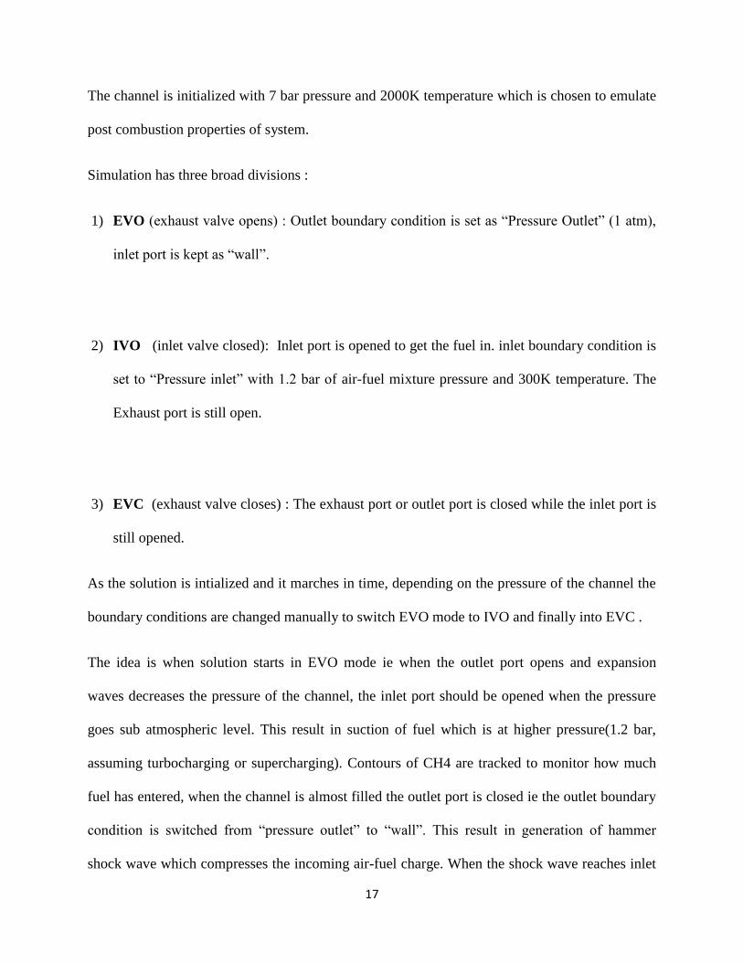
The channel is initialized with 7 bar pressure and 2000K temperature which is chosen to emulate

post combustion properties of system.

Simulation has three broad divisions :

1) EVO (exhaust valve opens) : Outlet boundary condition is set as “Pressure Outlet” (1 atm),

inlet port is kept as “wall”.

2) IVO (inlet valve closed): Inlet port is opened to get the fuel in. inlet boundary condition is

set to “Pressure inlet” with 1.2 bar of air-fuel mixture pressure and 300K temperature. The

Exhaust port is still open.

3) EVC (exhaust valve closes) : The exhaust port or outlet port is closed while the inlet port is

still opened.

As the solution is intialized and it marches in time, depending on the pressure of the channel the

boundary conditions are changed manually to switch EVO mode to IVO and finally into EVC .

The idea is when solution starts in EVO mode ie when the outlet port opens and expansion

waves decreases the pressure of the channel, the inlet port should be opened when the pressure

goes sub atmospheric level. This result in suction of fuel which is at higher pressure(1.2 bar,

assuming turbocharging or supercharging). Contours of CH4 are tracked to monitor how much

fuel has entered, when the channel is almost filled the outlet port is closed ie the outlet boundary

condition is switched from “pressure outlet” to “wall”. This result in generation of hammer

shock wave which compresses the incoming air-fuel charge. When the shock wave reaches inlet

18

of the channel, the simulation is stopped. The pre-combustion stage is achieved. This

methodology is represented in the following contour diagrams and pressure plots.

The left image is the pressure plot and the right image is pressure contour.

Figure 11 EVO : Burnt mixture is rushed out (time =0 )

Figure 12 Intermidiate Step of the EVO mode (time =.05ms)

19

Figure 13 The pressure at inlet falls below atmospheric pressure, the inlet port is opened now:

IVO (time =.164 ms)

Right hand side of image below represents the mole fraction contours of methane, the blue color

represents burnt gases.

Figure 14 The air-fuel mixture is sucked into the channel, the pressure inside the channel rises

up slightly (time = .193 ms)

20

Figure 15 The outlet port is closed : EVC (time = .455 ms)

Figure 16 The Shockwave reaches the inlet port resulting in precompression (time=.650 ms)

21

3.1 b) Post Processing of the simulation results

The work done by the gasses coming out from the channel is governed by unsteady flow physics.

To calculate the work done in each mode (EVO, IVO,EVC) the first law of thermodynamics is

used as applied to a control volume considering all transient terms.

This equation is integrated over time to find the workdone during exhaust stroke, compression

stroke and the fuel suction stroke. This is work done by the gases hence the positive sign of W

will indicate work output and negative sign will indicate work input.

22

Wc, We, and Ws represent the work done during compression (EVC), exhaust(EVO) and fuel

suction(IVO) stages.

To use above equations we need the properties of the flow at each time step. Therefore pressure,

density, entropy, temperature, mass flow rate, enthalpy, and total energy of the gases inside the

channel is averaged over entire volume and at required surface areas of control volume at each

time step. This data is then used estimate the work done by the gases and constructing cycle

diagrams.

23

Figure 17: P vs Specific Volume

24

Figure 18: Torque History

25

The P-ʋ (specific volume) is constructed by using average pressure and density values of

channel at each time step. Similarly torque history is recorded at each time step. As clear from

the graph the the torque output is an impulse acting over the channel. The peak of the impulse is

goverened by the channel shape and port timings. The quantitative results for the cycle are

summarized below :

Table 1: Quantitative results for the cycle

Wc -79.34 J

We 379.65 J

Ws 24.56 J

Q 949.2 J

Η 34.25 %

3.1 c) Port Timing Calculation

The port timing can be calculated if the rotational velocity (ω) of rotor is known. The ω can be

calculate dusing the energy balance for complete cycle. Wnet is the net work output of the cycle.

This value must be equal to the expression :-

= work done during one cycle over time interval T

or, Wnet =

ω = Wnet /

26

Wnet is calculated above and integral of torque (τ) over interval T can be calculated as the torque

history over time is known. This gives ω =

Table 2 : RPM

Ω 17000 rpm

1780.24 rad/s

Table 3 : Time History of the Cycle

t1 (EVO) 1.5 ms 7bar to below 1bar

t2 (IVO) 0.9 ms fuel in

t3 (EVC) 0.85 ms pre compression

t4 (IVC) 3.53 ms Combustion

T 7 ms time period

Table 4 : Angular History of the Cycle

ϴ1 = ω x t1 153 deg Exhaust Angle

ϴe = ϴ1 + ϴ2 =

244.8 deg

ϴ2 = ω x t2 91.8 deg

ϴ3 = ω x t3 86.7 deg Inlet Angle

ϴi = ϴ2 + ϴ3

=178.5 deg

ϴ4 = ω x t4 360 deg

27

The angular sizing of the ports is determined on the basis of the time intervals t1, t2, t3, and t4

which are governed by the result of numerical simulations. These values implicitly depends on

the aspect ratio chosen for the given channel. For rotor A aspect ratio Length / width = 5. With

radial length of the channel is 5 cm. Because of very high rpm requirement owing to low torque

output, the combustion should be timed such that ignition should start in next cycle, this implies

there is 1 power stroke in 2 revolution, one complete revolution is used for combustion.Hence

using the described approach rpm and exact required size of the rotor can be determined.

Inlet Angle Exhaust Angle

Figure 19 : Depiction of Inlet and Outlet angles

28

3.2 Analysis of Rotor B

Figure 20: 3D view for Rotor B

Figure 21: 2D Projection for a rotor channel

29

3.2 a) Similar Methodology is Applied to this rotor – simulation results

Figure 22: Sample image durung intermediate time step after exhaust port is opened

30

Figure 23: P-v diagram and the Torque History

31

3.2 b) Chronological Summary of Simulation

Table 5 : Cycle Summary from simulations

Mode (port-setting) Time Iteration number Average P and T

Intialization 0 0 7 bar, 2000K

EVO 0 0 7 bar, 2000K

IVO .91 ms 12204 .9 bar, 1200 K

EVC 1.65 ms 212204 1.2 bar, 481.7 K

Ignition 1.87 ms 23991 1.55 bar, 471 K

Table 6 : Quantitative results for the cycle

Wc 17.55 J

We 587.54 J

Ws 3.35 J

Q 1.108 kJ

Η 54.45 %

32

As calculated above the rotational speed is determinjed as :-

ω = Wnet /

Table 7: RPM

Ω 10,963 rpm

1148 rad/s

Table 8 : Time History of the Cycle

t1 (EVO) .91 ms 7bar to below 1bar

t2 (IVO) .74 ms fuel in

t3 (EVC) .20 ms pre compression

t4 (IVC) 3.62 ms Combustion Time

T (1.85 + 3.62) = 5.47 ms time period

Table 9: Angular History of the Cycle

ϴ1 = ω x t1 59.86 deg Exhaust Angle

ϴe = ϴ1 + ϴ2 =

108.53 deg

ϴ2 = ω x t2 48.68 deg


ϴi = ϴ2 + ϴ3

=61.83 deg

ϴ4 = ω x t4 238.32 deg

33

3.2 c) Simulations for RotorB with prescribed ω

The simulations so far were carried out without considering the angular velocity. The simulations

are carried out with respect to the frame of motion of the rotor channel itself. Hence it is worth

while to investigate the role of centrifrugal forces in the overall thermodynamics of the cycle. To

investigate this a frame motion equivalent to 5000 rpm is given to the mesh. The result are

summarised below


Wc 17.55 J

We 587.54 J

Ws 3.35 J

Q 1.13 kJ

Η 53.45 %

Table 11: Cycle Summary from simulations



EVO 0 0 7 bar, 2000K

IVO .89 ms 12140 .9 bar, 1200 K

EVC 1.54ms 20160 1.2 bar, 481.7 K

Ignition 1.75 ms 24270 1.55 bar, 471 K

34

From the comparision of the work done and efficiency number it is concluded that the

centrifugal forces doesnot affect the overall thermodynamic cycle of the engine.

ω = Wnet /

Table 12: RPM

Ω 10,963 rpm or 1148 rad/s

Table 13: Time History of the Cycle





T (1.74 + 3.73) = 5.47 ms time period



ϴe = ϴ1 + ϴ2 =

101.3 deg

ϴ2 = ω x t2 42.76 deg


ϴi = ϴ2 + ϴ3

=55.9 deg

ϴ4 = ω x t4 245.55 deg

35

But from the above tables it is infered that although the centrifugal force doesnot play a

significant role in influencing the overall thermodynamic cycle, it affects the time interval during

EVO, IVO, and EVC phases hence plays a role in influencing final angular shapes of the ports.

Therefore it is concluded that to obtain the final port-timings for a rotor a second simulation with

correct ω is required.

36

3.3 Analysis of Rotor C

Figure 24 : Sample image right before exhaust port is opened

37

Figure 25 : P-v and T-s Diagram

38

Figure 26: Torque History

39

3.3 a) Chronological Summary of Simulation

Table 15: Cycle Summary from simulations



EVO 0 0 7 bar, 2000K

IVO .99 ms 13680 .9 bar, 1200 K

EVC 1.52 ms 20680 1.2 bar, 481.7 K

Ignition 1.87 ms 25959 1.55 bar, 471 K

Table 16 : Quantitative results for the cycle

Wc 0.0032 J

We 1274 J

Ws -500.20 J

Q 1.70 kJ

Η 46.9 %

40

As calculated above the rotational speed is determinjed as :-

ω = Wnet /

Table 17: RPM

Ω 87933 rpm or 920.83 rad/s






T (1.87+4.95) =6.82 ms time period



ϴe = ϴ1 + ϴ2 =

80.19 deg

ϴ2 = ω x t2 28.0deg


ϴi = ϴ2 + ϴ3

=46.43 deg

ϴ4 = ω x t4 261.3 deg

41

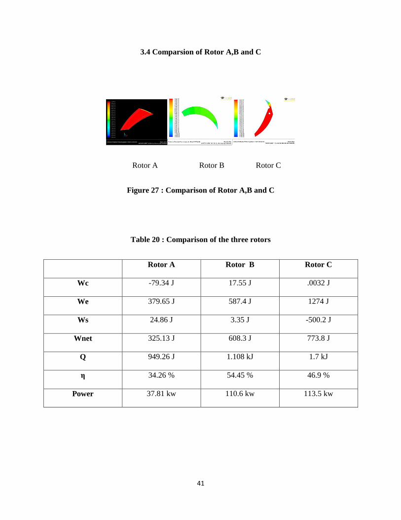
3.4 Comparsion of Rotor A,B and C

Rotor A Rotor B Rotor C

Figure 27 : Comparison of Rotor A,B and C

Table 20 : Comparison of the three rotors

Rotor A Rotor B Rotor C

Wc -79.34 J 17.55 J .0032 J

We 379.65 J 587.4 J 1274 J

Ws 24.86 J 3.35 J -500.2 J

Wnet 325.13 J 608.3 J 773.8 J

Q 949.26 J 1.108 kJ 1.7 kJ

η 34.26 % 54.45 % 46.9 %

Power 37.81 kw 110.6 kw 113.5 kw

42

Figure 28 :Comparison of P-v diagram

43

3.4 a) Discussion

1. Rotor A is least efficient and has least power output. This is owing to the fact that mass

flow rate at outlet is not restricted hence lot of mass goes out at a higher total enthalpy

without exchanging energy. This is illustrated from following figures.

2. Rotor C has superior torque output owing to the convergig-diverging shape of outlet.

Though the complicated channel shape results in alomost zero precompression

3. Rotor B is most efficient, although the power output is low comparative to rotor C but

owing to lesser torque output it will result in more losses in real world operations.

4. The power output can be increased if the gases exiting at outlet can further be expanded

via external turbines.

Figure 29: Torque-History of all three rotors

44

Figure 30: Mass-flow-rate at the outlet of the rotors.

45

3.5 Modified Rotor A

Figure 31: 3D view of Rotor A- with external row of turbine

To simulate the complete cycle for one given channel a simplified passage of rotor channel guide

vane and turbine channel is meshed. The figure below depicts the simplified 2D mesh.

46

Figure 32: Modified Rotor Channel with external channel

47

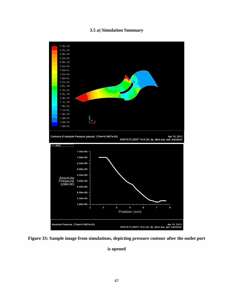
3.5 a) Simulation Summary

Figure 33: Sample image from simulations, depicting pressure contour after the outlet port

is opened

48

Figure 34 : P-v ans T-s Diagram

Figure 35 : Torque History

49

3.5 b) Chronological Summary of Simulation

Table 21 : Cycle Summary from simulations



EVO 0 0 7 bar, 2000K

IVO .532 ms 17500 .9 bar, 1200 K

EVC 1.12 ms 28370 1.2 bar, 481.7 K

Ignition 1.7 ms 38570 1.55 bar, 471 K


Wc -97.60 J

We 1223 J

Ws -701..02J

Q 950 kJ

Η 37.31 %

50

In addition work done by external turbine = mass flow rate at outlet of rotor *(total enthalpy at

rotor outlet-total enthalpy at turbine outlet) = 58.34 J. This gives net work output of 412.79 J.

Hence the effective efficiency is 43.45 %

As calculated above the rotational speed is determinjed as :- ω = Wnet /

Table 23: RPM

Ω 17000 rpm

1780.24 rad/s






T 3.53 ms time period

Table 25: Angular History of the Cycle


ϴe = ϴ1 + ϴ2 =

155.04

ϴ2 = ω x t2 54.1 deg


ϴi = ϴ2 + ϴ3

=89.8 deg

ϴ4 = ω x t4 360 deg

51

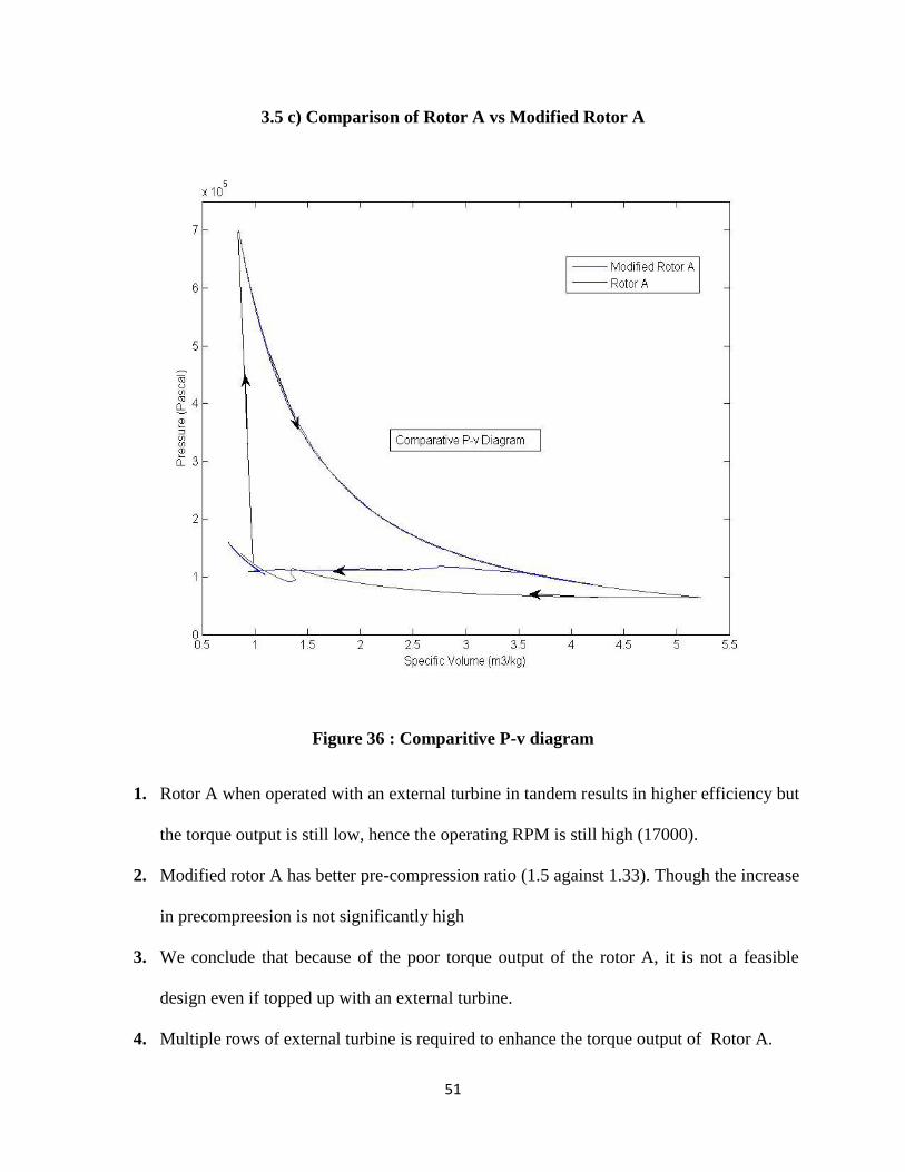
3.5 c) Comparison of Rotor A vs Modified Rotor A

Figure 36 : Comparitive P-v diagram

1. Rotor A when operated with an external turbine in tandem results in higher efficiency but

the torque output is still low, hence the operating RPM is still high (17000).

2. Modified rotor A has better pre-compression ratio (1.5 against 1.33). Though the increase

in precompreesion is not significantly high

3. We conclude that because of the poor torque output of the rotor A, it is not a feasible

design even if topped up with an external turbine.

4. Multiple rows of external turbine is required to enhance the torque output of Rotor A.

52

Chapter 4 : Conclusion and Future work

• Converging shape of rotor channel enhances thermal efficiency by creating stronger

compression waves.

• Torque output is more when a C-D outlet shape is chosen, this weakens the compression

wave.

• Therefore a rotor channel shape is a subject of optimization by balancing this two

competing phenomena

• Current methodology is a handy tool in comparing different rotor shapes.

• The methodology can be further refined by including gradual valve opening limitations,

effect of viscosity, heat losses across non adiabatic wall, and integrating simulation with

combustion models

• Practical Designs of wave rotor based machines are badly impacted by leakage.

53

REFERENCES

54

REFERENCES

[1] Anderson, John, 1995, Computational Fluid Dynamics: the Basics with Applications,

McGraw-Hill Science/Engineering/Math

[2] Akbari, P., Nalim, M. R., Mueller, N., “A Review of Wave Rotor Technology and Its

Applications,” ASME Journal of Engineering for Gas Turbines and Power, October 2006,

Vol. 128, pp. 717-735.

[3] Snyder, P., Alparslan, B., and Nalim, M. R., “Gas Dynamic Analysis of the Constant Volume

Combustor, A Novel Detonation Cycle,” AIAA Paper 2002-4069, 2002.

[4] Paxson D. E.,1996, "Numerical Simulation of Dynamic Wave Rotor performance," AIAA

Journal of Propulsion and Power, Vol. 12, No. 5, pp.949-957, (also, NASA TM 106997).

[5] Paxson D. E., 1995, “A Numerical Model for Dynamic Wave Rotor Analysis,” AIAA Paper

95-2800. Also NASA TM-106997.

[6] Akbari, P. and Nalim, M. R., “Review of Recent Developments in Wave Rotor Combustion

Technology.” Journal of Propulsion and Power, Vol. 25, No. 4, pp 833-844, July–August

2009.

[7] Iancu. F, Piechna. J, Dempsey. E, and Müller. N, “The Ultra-Micro Wave Rotor Research a t

Michigan State University, second International Symposium on Innovative Aerial/Space

Flyer Systems, The University of Tokyo, 2005, pp 65–70.

Documents

DEVELOPMENT OF METHODOLOGY FOR DESIGNING WAVE DISK …