1

Development of New Grid-Fin Design for Aerodynamic Control

Marco Debiasi1 Temasek Laboratories, National University of Singapore, Singapore, 117411

A swept-back grid-fin with sharp leading edges has been developed for reducing the drag associated to the choking of the flow in the lattice cells at transonic speeds. Computational fluid dynamic simulations and experimental measurements at transonic and supersonic speeds and zero angle of attack indicate a 30% drag reduction compared to a standard grid-fin type. Additional windtunnel measurements have been performed at selected freestream conditions by varying the angle of attack of the ogive-cylinder body used to support the grid fins. The results provide information on the control authority of the grid fins and indicate that the swept-back with sharp leading edges type has equal or better control characteristics than the standard type.

Nomenclature CF = force coefficient CM = moment coefficient c = grid-fin chord (lattice element chord) D = diameter of the ogive-cylinder body F = force h = grid-fin height L = length of the ogive-cylinder body M∞ = freestream Mach number p = static pressure ReD = Reynolds number based on the body diameter s = grid-fin span T = static temperature

U∞ = freestream velocity w = thickness of the walls of the lattice cells x = longitudinal coordinate of the vehicle y = spanwise coordinate of the vehicle z = normal coordinate of the vehicle Greek letters = angle of attack = angle of the sharp leading edge = swept-back angle

I. Introduction grid fin is an aerodynamic control surface consisting of an outer frame with an internal lattice of

intersecting thin walls of small chord. Unlike conventional planar fins, that are aligned parallel to the direction of the airflow, grid fins are mounted perpendicular to the flow allowing the oncoming air to pass through the cells of the lattice.

Contents of this paper were previously presented as Paper 2010-4244 at the 28th AIAA Applied Aerodynamics Conference, Chicago, Illinois, 28 June - 1 July 2010, and as Paper 2012-2909 at the 30th AIAA Applied Aerodynamics Conference, New Orleans, Louisiana. 25 - 28 June 2012. 1 Senior Research Scientist, Temasek Laboratories, National University of Singapore, Singapore.

A

2

The main advantage of grid fins is that they have significantly smaller chord than conventional planar fins. Thus, they generate smaller hinge moments which require smaller actuators to rotate them in a high-speed flow. Their small chord also makes them less likely to stall at high angles of attack which increases their control effectiveness compared to conventional planar fins. Another advantage of grid fins is that they can be folded easily against an aerodynamic body to make them more compact and convenient to store or transport.

Both theoretical and experimental studies have been performed on grid fins. The first investigation on grid fin aerodynamics was carried out by Belotserkovskiy et al.1 by using a theoretical method which relies mainly on empirical formulas. Burkhalter et al. used the vortex lattice approach to analyze the grid-fin flow in the subsonic regime.2 Washington et al.3 conducted windtunnel experiments to study the aerodynamic effects of fin curvature and angle of protrusion from the body at some subsonic and supersonic Mach numbers. Their data indicate that “fin curvature has small effect on fin normal force, hinge moment, and bending moment”. Miller and Washington4 extended the experiments to study the effects on drag of the cross-section shape of the outer-frame walls and of the thickness of the walls of the lattice cells. Their findings indicate that simple shaping of the cross section of the frame, reduction of the wall thickness, or a combination thereof can considerably reduce drag levels with minimal impact on the grid-fin lift and other aerodynamic properties. Later experimental works by Abate et al.5 and by Fournier6,7 focus on the overall aerodynamic performance of an ogive-cylinder body with grid fins.

The studies above rely mainly on measurements of the force and moment from individual fins and from the whole vehicle (i.e. an aerodynamic body with fins). However, no attempt was made to resolve in detail the flow inside and around the lattice cells. Recently Theerthamalai and Nagarathinam8 developed a prediction method for the estimation of the aerodynamic characteristics of grid-fins at supersonic Mach numbers. The shock and expansion relations and the interactions between the shock and expansion waves were used to predict the pressure distribution inside each grid-fin cell.

Besides theoretical and experimental studies, computational fluid dynamics (CFD) has been used for investigating the aerodynamic characteristics of grid fins. Chen et al.9 simulated an ogive-cylinder body with grid fins by using the NPARC code of NASA. The issue of the grid-fin size, in terms of both the walls thickness and the frontal shape of the lattice was addressed. Lin et al.10 computed the turbulent flows past a grid fin alone and past various fin/body combinations at Mach numbers of 0.7 and 2.5. The results provide the detailed flow fields including Mach-number contours, pressure contours, and streamline patterns as well as the integrated aerodynamic coefficients. DeSpirito and Sahu11 conducted CFD studies by using the commercial CFD code FLUENT with the objective of investigating what advantages grid fins offer over conventional planar fins. Good agreement was observed between the CFD data and the aerodynamic coefficients measured in tests of an ogive-cylinder body with grid fins conducted in the windtunnel of the Defence Research Establishment, Valcartier (DREV), Canada.7 The simulations successfully captured the flow structure around the fin in the separated-flow region at the higher angles of attack.

Depending on the speed of the airflow, grid fins can have a higher or lower drag compared to conventional planar fins.5, 6 The drag and the control characteristics of a grid fin at low subsonic speeds are similar to those of a planar fin since the thin walls create very little disturbance in the flow of air passing through the lattice. However, the same behavior does not hold true in the transonic regime. Hughson et al.12,13 used CFD to investigate the transonic flow fields about and through the cells of a vehicle with lattice grid fins. The results illustrate that at transonic Mach numbers a normal shock forms at the back of the grid cells. The flow inside the cells chokes thus reducing the flow rate through the lattice which effectively acts as an obstacle to the flow. A normal shock then develops in front of the grid fin with attendant drag increase. At higher speed, this shock is swallowed by the lattice thus reducing the drag and improving the control characteristics.

The main objective of the research presented here is the reduction of grid-fin drag in the transonic regime. A modified configuration consisting of a swept-back grid fin with sharp leading edges (SB-sharp) has been proposed in previous studies.14,15 The merit of this design was evaluated by comparing it, both numerically and experimentally, to a standard grid-fin design well documented in literature. The results obtained at zero angle of attack indicate that drag reductions of about 30% can be achieved in the transonic regime. Additional windtunnel measurements have been performed at selected freestream Mach numbers by varying the angle of attack of the ogive-cylinder body supporting the fins. These provide a preliminary assessment of the characteristics of the swept-back grid fins with sharp leading edges as control surfaces. The data obtained are also useful for preparing a future study specifically addressing the performance of SB-sharp fins placed at deflected angles with respect to the body centerline and the properties of swept-forward grid fins with sharp leading edges which offer some additional advantages in practical applications.

II. Grid-fin Configurations The standard grid-fin geometry investigated by Abate et al.5, DeSpirito and Sahu,11 and Hughson et al.12,13,

Figs. 1a) and 1b), has been selected as the baseline configuration in the current study. All the dimensions in Fig. 1 are relative to the diameter D of the ogive-cylinder body. This consists of a 3D long tangent ogive nose with a

3

7D long cylindrical afterbody with four grid fins mounted in a cruciform orientation. The pitch axis of the grid fins is located 1.5D from the rear of the cylinder. The grid fin has a rectangular-shaped outer frame with span s, height h and chord c of size 0.75D, 0.333D and 0.118D respectively. The thickness w of the walls of the lattice is 0.007D.

Fundamental aerodynamic considerations similar to those presented by Guyot and Schülein16, as well as in the design of transonic and supersonic inlets, suggest that adding a swept-back angle to the fin lattice should improve its drag characteristics. The grid-fin geometry has been modified accordingly by sweeping back the frameworks of grid cells along the chord direction with the same projected structure and dimensions as shown in Fig. 1a). Figure 1c) shows the top view of the swept-back grid fin configuration (SB) whose swept-back angle is = 30°. The swept back angle also slightly staggers the leading edges of the lattice with respect to each other. This in conjunction with adding sharp leading edges (SB-sharp) improves the flow ingestion by the lattice at transonic and supersonic speeds, as illustrated in Fig. 2. The angle of the sharp leading edges is 20°, i.e. the same value used in the configuration studied by Guyot and Schülein.16

III. Experimental Setup Experiments were conducted to measure the aerodynamic characteristics of the ogive-cylinder body with the

baseline and the SB-sharp grid fins. To this aim, models of the grid fins were fabricated and tested in a transonic windtunnel. The models are made of stainless steel, Fig. 3, and their dimensions are s = 85.7 mm, h = 38.1 mm, c = 13.5 mm, and w = 0.8 mm, Fig. 1. The fins were installed at 1.5D from the rear of the cylindrical body of an AGARD-C model which has L/D = 10. In order to better discriminate the drag of the fins, the wings and the empennage of the AGARD-C model were removed and replaced by plugs flush-mounted with the surface of the body. The body was mounted on a sting in the center of the windtunnel test section. The minimum distance of the fin tips from the test-section walls was more than 3 times the fin span thus wall interference and blockage effects were negligible. A balance located close to the center of gravity of the ogive-cylinder body and with a resolution of 0.014N and an accuracy of 0.092% was used to measure the forces and moments acting on the body. These data were measured and recorded simultaneously to the total and static values of the pressure and temperature in the test section.

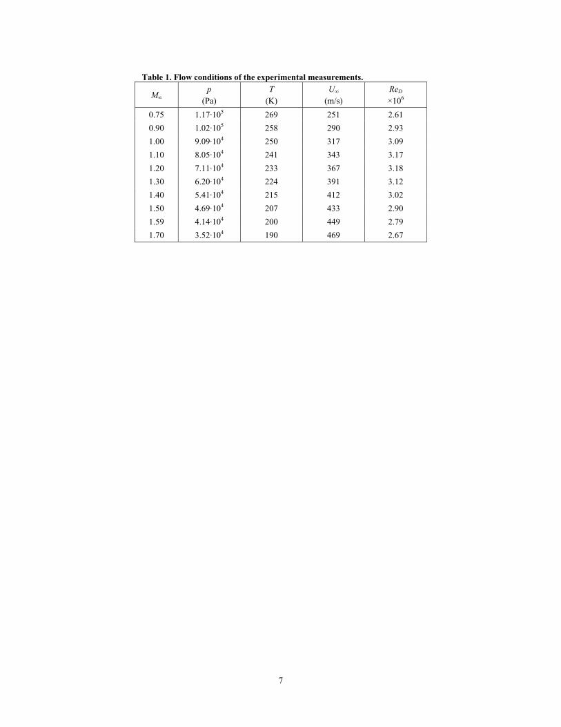
Experimental measurements were taken at freestream Mach numbers M∞ between 0.75 and 1.7. The windtunnel is of the blow-down type and incorporates a control system that maintains the Mach number and the pressure in the test section within 1% of the desired values. The variation of the temperature during the experiments was negligible due to the short duration of each run and to the use of a heat exchanger that minimizes the temperature drop with the depletion of the air in the reservoir. The corresponding static pressure p and the static temperature T in the test section vary as indicated in Table 1.

Two series of experimental measurements were performed. The first series focused on drag measurements for which the freestream velocity was explored in detail with the model at zero angle of attack. The second series explored the effect of the angle of attack of the model at selected freestream Mach numbers. Based on data from the first series of measurements, M∞ = 0.90, 1.09, and 1.30 were selected as the most significant freestream conditions to investigate. At each Mach number, the angle of attack was varied from 0° to 12° during each run. Measurements were taken both for the baseline and the SB-sharp fins by mounting all the four fins on the body or by mounting only the lateral (elevators) fins. This was done to gain some insight of the aerodynamic contribution of the lateral fins decoupled from that of the vertical (rudder) fins.

IV. Numerical Simulations The process used to create the meshes for the numerical simulation, the governing equations and the flow

solver used, and the boundary conditions adopted are described in Zeng et al.14 and Debiasi et al.15 which can be used as a reference for a detailed description. It suffices here to recall that by taking advantage of the model symmetry at zero angle of attack, only one quarter of the geometry was used for the calculation domain in the CFD study. The upstream and downstream boundaries are located 12D away from the nose and tail of the ogive-cylinder body, and radially 16D away from the cylinder surface. Far-field pressure boundary conditions were applied for the outer boundaries, symmetry conditions for the symmetry surfaces, and non-slip conditions for all the solid surfaces. The total number of grid cell elements for the computational domain is about 1.2 million. 3D Navier-Stokes equations coupled with the Spalart-Allmaras one-equation turbulence model were used to simulate the turbulent flow field and the CFD software FLUENT was chosen to compute the flow. The results were tracked to ensure their convergence. Parallel computing was used to speed up the computations. A complete parallel simulation run in 8 processors and took approximately 120 CPU hours. When possible, our numerical simulations have been validated by comparing the results with equivalent data available in literature. The data obtained indicate that our simulations match quite well the results from other research groups.14,15

4

V. Results The forces and moments reported here are relative to the center of the balance which is located close to the

center of the AGARD-C body and whose coordinate system has x axis in the longitudinal direction, y axis in the spanwise direction, and z axis normal to these. The forces and moments exerted by the fins were obtained as the difference of those of the AGARD-C body with fins and without them at the same flow conditions. No significant differences were found between repeated measurements.

A. Drag measurements at zero angle of attack Figure 4 presents the values of the axial force (i.e. the drag) Fx,fin of the baseline and of the SB-sharp fins

from experimental measurements at = 0° for freestream Mach numbers between 0.75 and 1.7. For both fins the axial force increases with the freestream velocity and reaches a maximum at about M∞ = 1.1 after which is gently decreases. This is consistent with the choking of the flow in the lattice cells at transonic conditions. At this Mach number the maximum axial force measured for the baseline fin is 88 N whereas the maximum axial force measured for the SB-sharp fin is 62 N at M∞ = 1.05. It should be noted that the axial force of the SB-sharp fin is more than 20 N lower than the axial force of the baseline fin across the whole Mach range explored.

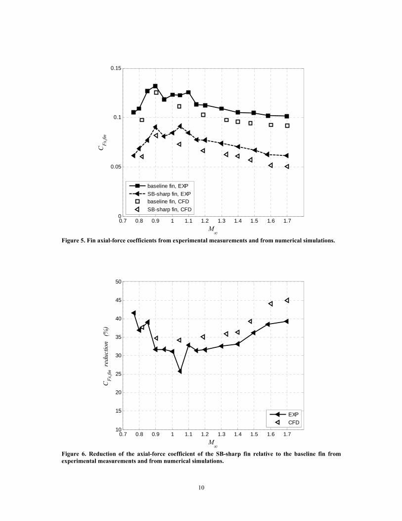
Figure 5 reports the corresponding values of the axial-force coefficient CFx,fin of one fin. This was obtained by using 1/4 of the base of the AGARD-C cylindrical body as the reference area and its diameter as the reference length. Figure 5 presents also the corresponding values of the axial-force coefficient from numerical simulations (CFD). The numerical simulations seem to underestimate the value of the axial-force coefficient by about 10% compared to the experiments. This discrepancy may be caused by the presence of the sting support which is not modeled in the simulations since these were meant to be comparable to previous CFD works and to data from ballistic range measurements, all of which do not include a supporting sting. Notwithstanding this discrepancy, it should be noted that the values of CFx,fin from CFD and from the experiments follow the same trend.

Figure 6 presents the corresponding reduction of the axial-force coefficient (percent benefit) offered by the SB-sharp fin compared to the baseline type together with the corresponding values from the numerical simulations. The experiments substantially confirm the results of the numerical simulations and indicate that, compared to the baseline fin, the drag of the SB-sharp fin is reduced by more than 30% in the Mach range explored with the possible exception of a smaller reduction (25%) close to M∞ =1.1 where the drag is higher as discussed above. Additional measurements should be performed around this Mach number to confirm the dip observed in Fig. 6 for this flow condition.

Having verified that the results from the numerical simulations agree quite well with the wind-tunnel measurements, we utilize the numerical data to explore in more detail the features of the flow across the grid fins.

The flow fields through the baseline and the SB-sharp grid fins are fairly complex. Figures 7 to 9 show the detailed Mach number contours on the x-z plane passing through the baseline and the SB-sharp grid fins at M∞ = 1.045, 1.332, and 1.70, respectively. The walls of the baseline configuration have blunt leading edges which cause a local deceleration of the approaching flow. The boundary layer inside the cells, which grows from the leading edge, and the flow stagnating at the junctions of the walls introduce a decrease in the flow area. At M∞ = 1.045 the flow inside the cells of the baseline lattice is accelerated, Fig. 7a), thus reaching pressure values at the lattice exit that are not in balance with the pressure of the flow surrounding the fin. Thus the flow exiting the cells equalizes the pressure of the surroundings through a series of expansions and compressions. The X pattern past the lattice elements in Fig. 7a) clearly shows the expansion fans of the flow exiting the cells. When such expansions reach pressure values below the surrounding, they are followed by rather abrupt shocks across which the flow pressure matches the surroundings. These shocks create an arch past the fin cells. The energy dissipation associated with these processes limits the efficient passage of the flow through the lattice with attendant choking of the flow. The system of expansion fans and shocks from the SB-sharp configuration is similar, Fig. 7b), but the strength of these phenomena is reduced compared to the baseline case.

Similar observations can be drawn for the grid fins at M∞ = 1.332, shown in Figure 8. At this Mach number the normal shock in front of the SB-sharp fin is almost attached to the lattice, Fig. 8b), as opposed to the detached bow shock in front of the baseline fin, Fig. 8a), which worsens the drag by forcing additional air to spill around the fin.

At M∞ = 1.70, i.e. past the transonic regime, the flow characteristics of the baseline and SB-sharp cases are quite different, see Fig. 9. The strong shock in front of the baseline fin, Fig. 9a), induces large flow losses. The pressure of the flow past this strong shock rises at the expense of the velocity and the flow emerges at the exit of the cells with relatively low speed and higher pressure than the surroundings. Past the fin an expansion and shock structure similar to the lower speed cases is observed through which the flow pressure equalizes with the surroundings. The strong shock upstream of the baseline fin is replaced by oblique shocks at the leading edges of the SB-sharp fin, Fig 9b). The flow remains supersonic within the cells and weak expansion waves form at the trailing edge of the cells. Flow choking is notably absent and lower drag is obtained.

5

These observations support the design rationale of sweeping back the lattice of the grid-fins and of adding the 20° sharp leading edge to the swept-back lattice both of which are expected to reduce the losses and facilitate the passage of the flow though the lattice cells.

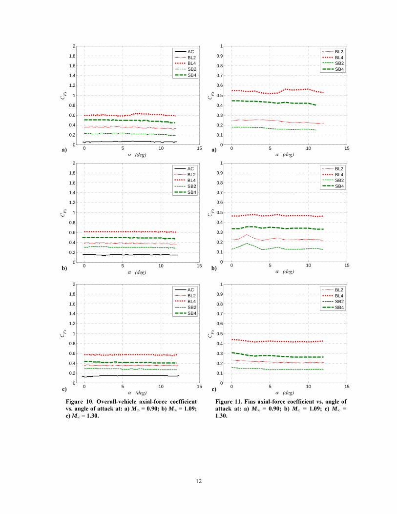
B. Force and moment measurements at non-zero angles of attack The aerodynamic effect of varying the angle of attack of the body was not simulated in this study as this

would have required doubling the size of the mesh (to reflect the symmetry along the vertical plane through the body center line as opposed to exploiting the axial symmetry for = 0°) and, correspondingly, the already significant computational time. Furthermore, insufficient CFD studies for 0° are available in literature to provide a reference for comparison of the numerical simulations. Accordingly, only experimental measurements were used to explore the effect of the angle of attack. These were performed by continuously varying from 0° to 12° (the highest angle at which the AGARD-C model could be set in the test section of the windtunnel) at M∞ = 0.90, 1.09, and 1.30 which are considered to be significant freestream conditions, see Fig. 4. Few measurements, not shown here, were performed by varying from 0° to -12° to verify that the results mirror those obtained at positive angles of attack, as expected.

The following acronyms are used in the successive figures to designate the data from the experimental measurements: AC is for the AGARD-C body alone (without fins), BL2 is for the body with only the two lateral (elevators) baseline fins, BL4 is for the body with all four baseline fins, SB2 is for the body with only the two lateral SB-sharp fins, and SB4 is for the body with all four SB-sharp fins.

Figures 10 and 11 show the axial-force coefficient of the overall vehicle and of the fins alone, respectively, as a function of the angle of attack . The axial-force coefficient is fundamentally insensitive of the angle of attack. The coefficient of the overall vehicle with baseline fins has value 0.6 at all the angles of attack which is close to the results reported in other studies 3,4,7,11 (some of which use slightly different baseline fins). Most important, the data confirm the drag benefit offered by the SB-sharp fins and indicate that it applies to a range of velocities and angles of attack relevant to a maneuvering vehicle.

Similarly, Figs. 12 and 13 show the normal-force coefficient of the overall vehicle and of the fins alone, respectively. The normal force increases with the angle of attack, this effects being larger for the body with fins. The body with baseline fins exhibits an almost linear increase of the normal-force coefficient with increasing values of whereas the coefficient of the body alone is lower but increases more than linearly with . These findings are consistent with the data available in literature for baseline fins.3,11 Interestingly, the SB-sharp fins have slightly higher normal-force coefficient than the baseline fins, indicating a somewhat better performance of the SB-sharp type for a maneuvering vehicle. This is especially evidenced by Fig. 13 which also indicates a smoother behavior of the SB-sharp type at subsonic speed. The values from Fig. 13 also compare quite well with the build-up of the normal-force coefficient of individual baseline fins reported by DeSpirito and Sahu for M∞ = 2.0.11

Figures 14 and 15 show the pitching-moment coefficient of the overall vehicle and of the fins alone, respectively. The pitching moment of the AGARD-C body increases with the angle of attack. The fins located at the tail of the body produce a negative pitching moment. This is consistent with the fins creating a positive normal force behind the center of the body where the balance is located. The values of the pitching-moment coefficient also compare quite well with those reported by DeSpirito and Sahu for M∞ = 2.0 once one takes into account that their values are relative to a reference point coinciding with the nose of a L/D = 16 body.11 That is, the arm of their moment is more than four times larger. Consistent with the normal-force values, the pitching-moment coefficient of the SB-sharp fins is slightly higher than the baseline fins, indicating a better performance of the SB-sharp type for a maneuvering vehicle. This is evidenced by Fig. 15 which also indicates the smoother behavior of the SB-sharp type at subsonic speed.

The measured lateral-force, roll-moment, and yaw-moment are very small at all speeds, as expected when only the angle of attack of the body is varied. Accordingly, the corresponding coefficients are negligible and are not presented here.

VI. Conclusion Flow choking usually occurs in the lattice cells of standard grid fins at transonic flight conditions, which

causes a significant increase of the drag force. To reduce this problem an improved grid-fin design has been proposed which combines a 30° swept-back lattice structure with sharp leading edges of the cells walls. The merit of using this design for reducing the drag has been evaluated by comparing it, both numerically and experimentally, to a baseline standard design well documented in literature. To this aim the flow over an ogive-cylinder body with baseline and swept-back with sharp leading edges (SB-sharp) grid fins was investigated at freestream Mach number ranging from 0.75 to 1.7 with the body at zero angle of attack. The results indicate that the SB-sharp fins have a drag coefficient about 30% lower than the baseline fins. Additional experimental

6

measurements provide a preliminary assessment of the efficacy of the SB-sharp fins as aerodynamic control surfaces. To this aim, the aerodynamic characteristics of the fins have been measured in a transonic windtunnel by varying the angle of attach of the body supporting them. The data obtained at selected freestream Mach numbers indicate that the drag benefit of the SB-sharp fins is maintained at non-zero angles of attack and that the control qualities of the SB-sharp fins are equal or better than those of the baseline fins. These results are encouraging and relevant to the use in maneuvering vehicles. While the results obtained suggest several advantages of using SB-sharp fins in place of standard grid fins, the benefit of the SB-sharp fins compared to conventional planar fins has not been addressed. At the same time, no data were obtained on the performance of the SB-sharp fins placed at deflected angles with respect to the body centerline. These will be explored in a future study that will also consider the properties of swept-forward grid fins with sharp leading edges.

References 1Belotserkovskiy, S. M., Odnovol, L. A., et al., “Wings with Internal Framework,” Machine Translation FTD-ID (RS) T

1289, Foreign Technology Division, Feb. 1987. 2Burkhalter, J. E., Hartfield, R. J., and Leleux, T. M., “Nonlinear Aerodynamic Analysis of Grid Fin Configuration,”

Journal of Aircraft, Vol. 32, No. 3, 1995, pp. 547-554. 3Washington, D., Booth, P. F., and Miller, M. S., “Curvature and Leading Edge Sweep Back Effects on Grid Fin

Aerodynamic Characteristics,” AIAA Paper 93-3480. 4Miller, M. S., and Washington, D., “An Experimental Investigation of Grid Fin Drag Reduction Techniques,” AIAA

Paper 94-1914, 12th AIAA Applied Aerodynamics Conference, Colorado Springs, CO, 20-22 June 1994. 5Abate, G., Winchenbach, G., and Hathaway, W., “Transonic aerodynamic and scaling issues for lattice fin projectiles

tested in a ballistic range,” Proceedings of the 19th International Symposium of Ballistic, Interlaken, Switzerland, 7-11 May 2001, pp. 413-420.

6Fournier, E. Y., “Wind tunnel investigation of a high L/D projectile with grid fin and conventional planar control surfaces,” Proceedings of the 19th International Symposium of Ballistics, Interlaken, Switzerland, 7-11 May 2001, pp. 511-520.

7Fournier, E. Y., “Wind Tunnel Investigation of Grid Fin and Conventional Planar Control Surfaces,” AIAA Paper 2001-0256, 39th AIAA Aerospace Sciences Meeting and Exhibit, Reno, NV, 8-11 January 2001.

8Theerthamalai, P., and Nagarathinam, M., “Aerodynamic Analysis of Grid-Fin Configurations at Supersonic Speeds,” Journal of Spacecraft and Rockets, Vol. 43, No. 4, 2006, pp. 750-756.

9Chen, S., Khalid, M., Xu, H., and Lesage, F., “A Comprehensive CFD Investigation of Grid Fins as Efficient Control Surface Devices,” AIAA Paper 2000-0987, 38th AIAA Aerospace Sciences Meeting and Exhibit, Reno, NV, 10-13 January 2000.

10Lin, H., Huang, J. C., and Chieng, C-C., “Navier–Stokes Computations for Body/Cruciform Grid Fin Configuration,” Journal of Spacecraft and Rockets, Vol. 40, No. 1, 2003, pp. 30-38.

11DeSpirito, J., and Sahu, J., “Viscous CFD Calculations of Grid Fin Missile Aerodynamics in the Supersonic Flow Regime,” AIAA Paper 2001-0257, 39th AIAA Aerospace Sciences Meeting and Exhibit, Reno, NV, 8-11 January 2001.

12Hughson, M. C., Blades, E. L., and Abate, G. L., “Transonic Aerodynamic Analysis of Lattice Grid Tail Fin Missiles,” AIAA Paper 2006-3651, 24th AIAA Applied Aerodynamics Conference, San Francisco, California, 5-8 June 2006.

13Hughson, M. C., Blades, E. L., Luke, E. A., and Abate, G. L., “Analysis of Lattice Grid Tailfin Missiles in High-Speed Flow,” AIAA Paper 2007-3932, 25th AIAA Applied Aerodynamics Conference, Miami, FL, 25-28 June 2007.

14Zeng, Y., Cai J. S., Debiasi, M., and Chng, T. L., “Numerical Study on Drag Reduction for Grid-Fin Configurations,” AIAA Paper 2009-1105, 47th AIAA Aerospace Sciences Meeting and Exhibit, Reno, NV, 5-8 January 2009.

15Debiasi, M., Zeng, Y., and Chng, T. L., “Swept-back Grid Fins for Transonic Drag Reduction,” AIAA Paper 2010-4244, 28th AIAA Applied Aerodynamics Conference, Chicago, IL, 28 June - 1 July 2010.

16Guyot, D., and Schülein, E., “Novel Locally Swept Lattice Wings for Missile Control at High Speeds,” AIAA Paper 2007-0063, 45th AIAA Aerospace Sciences Meeting and Exhibit, Reno, NV, 8-11 January 2007.

7

Table 1. Flow conditions of the experimental measurements.

M∞ p

(Pa) T

(K) U∞

(m/s) ReD

×106

0.75 1.17·105 269 251 2.61

0.90 1.02·105 258 290 2.93

1.00 9.09·104 250 317 3.09

1.10 8.05·104 241 343 3.17

1.20 7.11·104 233 367 3.18

1.30 6.20·104 224 391 3.12

1.40 5.41·104 215 412 3.02

1.50 4.69·104 207 433 2.90

1.59 4.14·104 200 449 2.79

1.70 3.52·104 190 469 2.67

8

a)

b) c)

Figure 1. Schematic of the grid-fin configurations: a) front view of the grid-fin structure; b) top view of the baseline grid fin; c) top view of the swept-back grid fin.

Figure 2. Schematic of the flow approaching a standard, blunt-leading-edged cell (left) and a swept-back, sharp-leading-edged cell (right).

w = 0.007 0.1109

s = 0.750

h = 0.333

c = 0.118

h = 0.333

c = 0.118

h = 0.333

9

Figure 3. Grid-fin models for experimental measurements in the windtunnel: standard flat configuration from Hughson et al.11 (baseline for this study; left) and swept-back with sharp leading edges configuration (SB-sharp; right).

0.7 0.8 0.9 1 1.1 1.2 1.3 1.4 1.5 1.6 1.70

10

20

30

40

50

60

70

80

90

100

M

Fx,

fin

(N)

baseline fin

SB-sharp fin

Figure 4. Fin axial force from experimental measurements.

10

0.7 0.8 0.9 1 1.1 1.2 1.3 1.4 1.5 1.6 1.70

0.05

0.1

0.15

M

CF

x,fin

baseline fin, EXP

SB-sharp fin, EXPbaseline fin, CFD

SB-sharp fin, CFD

Figure 5. Fin axial-force coefficients from experimental measurements and from numerical simulations.

0.7 0.8 0.9 1 1.1 1.2 1.3 1.4 1.5 1.6 1.710

15

20

25

30

35

40

45

50

M

CF

x,fin

red

uctio

n (

%)

EXP

CFD

Figure 6. Reduction of the axial-force coefficient of the SB-sharp fin relative to the baseline fin from experimental measurements and from numerical simulations.

11

Figure 7. Mach number contours on the x-z plane of vertical (rudder) fins at M∞=1.045: a) baseline fin; b) SB-sharp fin.

M

1.71

0.00

0.86

1.28

0.43

a) b)

a) b)

1.81

0.00

0.91

1.36

0.46

M

Figure 8. Mach number contours on the x-z plane of vertical (rudder) fins at M∞=1.332: a) baseline fin; b) SB-sharp fin.

a) b)

1.71

0.00

0.86

1.28

0.43

M

Figure 9. Mach number contours on the x-z plane of vertical (rudder) fins at M∞=1.70: a) baseline fin; b) SB-sharp fin.

12

Figure 10. Overall-vehicle axial-force coefficient vs. angle of attack at: a) M∞ = 0.90; b) M∞ = 1.09; c) M∞ = 1.30.

Figure 11. Fins axial-force coefficient vs. angle of attack at: a) M∞ = 0.90; b) M∞ = 1.09; c) M∞ = 1.30.

0 5 10 150

0.2

0.4

0.6

0.8

1

1.2

1.4

1.6

1.8

2

(deg)

CF

x

ACBL2BL4SB2SB4

0 5 10 150

0.2

0.4

0.6

0.8

1

1.2

1.4

1.6

1.8

2

(deg)

CF

x

ACBL2BL4SB2SB4

0 5 10 150

0.2

0.4

0.6

0.8

1

1.2

1.4

1.6

1.8

2

(deg)

CF

x

ACBL2BL4SB2SB4

a)

b)

c)

0 5 10 150

0.1

0.2

0.3

0.4

0.5

0.6

0.7

0.8

0.9

1

(deg)

CF

x

BL2BL4SB2SB4

0 5 10 150

0.1

0.2

0.3

0.4

0.5

0.6

0.7

0.8

0.9

1

(deg)

CF

x

BL2BL4SB2SB4

0 5 10 150

0.1

0.2

0.3

0.4

0.5

0.6

0.7

0.8

0.9

1

(deg)

CF

x

BL2BL4SB2SB4

a)

b)

c)

13

Figure 12. Overall-vehicle normal-force coefficient vs. angle of attack at: a) M∞ = 0.90; b) M∞ = 1.09; c) M∞ = 1.30.

Figure 13. Fins normal-force coefficient vs. angle of attack at: a) M∞ = 0.90; b) M∞ = 1.09; c) M∞ = 1.30.

0 5 10 150

0.2

0.4

0.6

0.8

1

1.2

1.4

1.6

1.8

2

(deg)

CF

z

ACBL2BL4SB2SB4

0 5 10 150

0.2

0.4

0.6

0.8

1

1.2

1.4

1.6

1.8

2

(deg)

CF

z

ACBL2BL4SB2SB4

0 5 10 150

0.2

0.4

0.6

0.8

1

1.2

1.4

1.6

1.8

2

(deg)

CF

z

ACBL2BL4SB2SB4

a)

b)

c)

0 5 10 150

0.1

0.2

0.3

0.4

0.5

0.6

0.7

0.8

0.9

1

(deg)

CF

z

BL2BL4SB2SB4

0 5 10 150

0.1

0.2

0.3

0.4

0.5

0.6

0.7

0.8

0.9

1

(deg)

CF

z

BL2BL4SB2SB4

0 5 10 150

0.1

0.2

0.3

0.4

0.5

0.6

0.7

0.8

0.9

1

(deg)

CF

z

BL2BL4SB2SB4

a)

b)

c)

14

Figure 14. Overall-vehicle pitching-moment coefficient vs. angle of attack at: a) M∞ = 0.90; b) M∞ = 1.09; c) M∞ = 1.30.

Figure 15. Fins pitching-moment coefficient vs. angle of attack at: a) M∞ = 0.90; b) M∞ = 1.09; c) M∞ = 1.30.

0 5 10 15-3

-2

-1

0

1

2

3

(deg)

CM

y

ACBL2BL4SB2SB4

0 5 10 15-3

-2

-1

0

1

2

3

(deg)

CM

y

ACBL2BL4SB2SB4

0 5 10 15-3

-2

-1

0

1

2

3

(deg)

CM

y

ACBL2BL4SB2SB4

a)

b)

c)

0 5 10 15-4

-3.5

-3

-2.5

-2

-1.5

-1

-0.5

0

(deg)

CM

y

BL2BL4SB2SB4

0 5 10 15-4

-3.5

-3

-2.5

-2

-1.5

-1

-0.5

0

(deg)

CM

y

BL2BL4SB2SB4

0 5 10 15-4

-3.5

-3

-2.5

-2

-1.5

-1

-0.5

0

(deg)

CM

y

BL2BL4SB2SB4

a)

b)

c)