Development, Validation, Uptake Rate Modeling and …€¦ · costs of the sampler and ease of fabrication, the design allows for potential automation of ... 6.2.3 Vent pipe and HPV

Development, Validation, Uptake Rate

Modeling and Field Applications of a

New Permeation Passive Sampler

by

Suresh Seethapathy

A thesis

presented to the University of Waterloo

in fulfillment of the

thesis requirement for the degree of

Doctor of Philosophy

in

Chemistry

Waterloo, Ontario, Canada, 2009

©Suresh Seethapathy 2009

ii

AUTHOR'S DECLARATION

I hereby declare that I am the sole author of this thesis. This is a true copy of the thesis,

including any required final revisions, as accepted by my examiners.

I understand that my thesis may be made electronically available to the public.

iii

Abstract

Passive air sampling techniques are an attractive alternative to active air sampling because

of the lower costs, simple deployment and retrieval methods, minimum training

requirements, no need for power sources, etc.. Because of their advantages, passive

samplers are now widely used not only for water and indoor, outdoor and workplace air

analysis, but also for soil-gas sampling required for various purposes, including vapor

intrusion studies, contamination mapping and remediation.

A simple and cost effective permeation-type passive sampler, invented in our laboratory,

was further developed and validated during this project. The sampler is based on a 1.8 mL

crimp-cap gas chromatography autosampler vial equipped with a polydimethylsiloxane

(PDMS) membrane and filled with a carbon based adsorbent. Apart from the low material

costs of the sampler and ease of fabrication, the design allows for potential automation of

the extraction and chromatographic analysis for high-throughput analysis. The use of

highly non-polar PDMS reduces water uptake into the sampler and reduces early

adsorbent saturation. The thermodynamic properties of PDMS result in moderately low

sampling rate effects with temperature variations. Further, the use of PDMS allows for

easy estimation of the uptake-rates based on the physicochemical properties of the

analytes such as retention indices determined using capillary columns coated with PDMS

stationary phase.

In the thesis, the theoretical and practical aspects of the new design with regards to uptake

kinetics modeling and the dependence of the calibration constants on temperature,

humidity, linear flow velocity of air across the sampler surface, sampler geometry,

sampling duration, and analyte concentrations are discussed. The permeability of

polydimethylsiloxane toward various analytes, as well as thermodynamic parameters such

as the energy of activation of permeation through PDMS membranes was determined.

Finally, many applications of the passive samplers developed in actual field locations,

vital for the field validation and future regulatory acceptance are presented. The areas of

application of the samplers include indoor and outdoor air monitoring, horizontal and

vertical soil-gas contamination profiling and vapour intrusion studies.

iv

Acknowledgments

Firstly, I would like to extend profuse thanks to my research supervisor Dr. Tadeusz

Górecki for giving me the opportunity to work on this interesting project and making my

past few years at the University of Waterloo wonderful, challenging and interesting. I am

indebted to him for encouraging and guiding me not only to do true scientific work in the

laboratory, but also to present my research work at prestigious conferences in Europe and

in North America. This has resulted in my building acquaintances with leading scientists

in the field, understanding the hottest research areas, and as a bonus, improving my skills

in making presentations to the scientific community. On the research front, Dr. Górecki

has been extremely receptive of any new ideas while being rightfully critical on their

scientific merits and demerits. His methods of problem solving in the laboratory are

something I will use for the rest of my career.

I wish to thank Dr. James J. Sloan, Dr. Jean Duhamel and Dr. Jacek Lipkowski, members

of my advisory committee, for their helpful suggestions and critical review of my

graduate work.

I greatly appreciate the support and encouragement of Dr. Jacek Namieśnik, Dr. Bożena

Zabiegała and Dr. Monika Partyka at the Gdańsk University of Technology. The

discussions with them on passive sampling technology during my four week visit to

Gdańsk, Poland, have been very useful in further advancing my research at the University

of Waterloo.

My sincere thanks to the staff of the department of chemistry, especially Cathy Van Esch,

for guiding me smoothly through the administrative requisites during my graduate studies.

Jacek Szubra, Harmen Vander Heide, Andy Colclough and others at the Science

Technical Services have always been pleasant and helpful with anything I required to

build my experimental setup. My sincere thanks to them.

My special thanks to Todd McAlary, Hester Groenevelt, David Bertrand, Robin Swift,

Todd Creamer, Chapman Ross, Duane Graves, and many others at Geosyntec Consultants

for agreeing to test our invention at various field sites including those at Raritan Arsenal

v

at New Jersey, contaminated sites at Knoxville in Tennessee, Harvard university,

Maxxam school and Simmons residence at locations in Massachusettes, Thyez in France,

and various sites in Philippines, Mexico and Italy. I would like to extend my sincere

appreciation to Todd McAlary for giving me a glimpse of what large project management

is all about and for his relentless pursuit of commercialization of the passive sampling

technology developed within this project.

My thanks to Michael Dumas of Tauw scientifique and Birgitta Beuthe of SPAQuE SA,

both operating in Belgium, for chosing my passive samplers for a huge pollutant mapping

study at a contaminated site in Belgium. My special thanks to them for providing me with

crucial field data, which is perhaps the best proof for validation of the newly designed

passive samplers.

I would like to extend my heartfelt thanks to Dr. Alina Segal for being a constant

motivator to begin my endeavour at the University of Waterloo. The acknowldegment

will be incomplete without mentioning my special gratitudes to Ms. Maria Górecka, for

always being there for me and my wife, personally as well as professionally, throughout

our stay here at the University of Waterloo.

Timely help in numerous ways from past and present members of Dr. Górecki’s research

group is gratefully acknolwedged.

No amount of gratitude is enough to shower on my parents, brothers, sister, uncle

(Duraikannan Srinivasan), aunt (Parimala Duraikannan), cousins (Aravin and Anita) and

friends (Nandagopal Polamoda, Tom Blashill and Navin Madras) for all their support and

pride they have for me. The endeavor was certainly made easy due to the constant

motivation and support from Jyothi Thanigai, Athilesh Thanigai and Thanigai

Ranganathan.

Finally, I would like to thank my wife, Manjula, for not just motivating me to begin this

endeavor, but also for supporting me through all the ups and downs of the last few years.

She is truly the woman behind my successful completion of the degree.

vi

g{|á à{xá|á |á wxw|vtàxw àÉ Åç uÜÉà{xÜ? fâÇwtÜ fxxà{tÑtà{ç

vii

Table of Contents

List of Figures ......................................................................................................................... xiii

List of Tables ......................................................................................................................... xxii

List of Abbreviations ........................................................................................................... xxvii

1. Introduction and scope of the thesis ....................................................................................... 1

1.1 Active air sampling ......................................................................................................... 2

1.1.1Real-time pollutant measurement .............................................................................. 4

1.2 Passive sampling ............................................................................................................. 6

1.3 General principles of operation ....................................................................................... 8

1.3.1 Passive air sampling ............................................................................................... 10

1.3.2 Passive water sampling ........................................................................................... 14

1.4 Literature review ........................................................................................................... 14

1.5 Passive air samplers ...................................................................................................... 17

1.5.1 SUMMA™ canisters .............................................................................................. 17

1.5.2 3M™ Organic Vapor Monitor (OVM) 3500 sampler ............................................ 19

1.5.3 Solid-phase microextraction device ....................................................................... 20

1.5.4 Polyurethane foam passive sampler ....................................................................... 21

1.5.5 Other air samplers reported in literature ................................................................. 22

1.6 Passive soil gas sampling .............................................................................................. 25

1.6.1 GORE™ modules ................................................................................................... 25

1.6.2 PETREX sampling system ..................................................................................... 27

1.6.3 Seimpermeable membrane devices ........................................................................ 28

1.6.4 Solid-phase microextraction .................................................................................. 29

viii

1.6.5 Other samplers reported in literature ..................................................................... 29

1.7 Effect of environmental parameters .............................................................................. 30

1.7.1 Temperature ............................................................................................................ 30

1.7.2 Pressure ................................................................................................................... 31

1.7.3 Face velocity ........................................................................................................... 31

1.7.4 Sorbent strength, analyte concentration and humidity ........................................... 32

1.8 Performance reference compounds .............................................................................. 34

1.9 Passive sampling and regulatory guidelines/protocols ................................................ 36

1.10 Summary ...................................................................................................................... 38

1.11 Scope of the thesis ....................................................................................................... 39

2. Theory .................................................................................................................................. 41

2.1 Non-Ideal conditions ..................................................................................................... 43

2.1.1 Boundary layer width .......................................................................................... 44

2.1.2 Dynamics of the sampler response ...................................................................... 46

2.2 Estimation of the calibration constant ........................................................................... 48

2.2.1 Contribution of analyte partition coefficient to permeability .............................. 48

2.2.2 Relationship between the linear temperature-programmed retention index

and partition coefficient of the analyte ................................................................ 52

2.2.3 The calibration constant-LTPRI correlation ........................................................ 55

3. Experimental determination of the calibration constants and their correlation with

physicochemical properties of the analytes .......................................................................... 56

3.1 Background to original sampler design, development of the new design and

previous research observations ..................................................................................... 56

ix

3.2 Chemicals used in the experiments ............................................................................... 62

3.3 Experimental ................................................................................................................. 64

3.3.1 Passive sampler design ........................................................................................... 64

3.3.2 Experimental setup ................................................................................................. 68

3.4 Experimental methods .................................................................................................. 74

3.4.1 Determination of LTPRI ........................................................................................ 74

3.4.2 Determination of the calibration constants ............................................................ 75

3.4.2.1 Determination of analyte recovery rates from Anasorb 747® .................. 76

3.4.2.2 Determination of analyte mass in the samplers ....................................... 77

3.4.2.3 Determination of analyte concentrations in the calibration chamber ...... 80

3.5 Results and discussion .................................................................................................. 81

3.5.1 LTPRI of the different groups of model compounds ............................................. 81

3.5.2 Analyte recoveries from Anasorb 747® ................................................................. 83

3.5.3 Determination of membrane weight loss and interferences on extraction with

carbon disulphide ................................................................................................... 86

3.5.4 Calibration constants and their correlation with LTPRIs ....................................... 87

3.5.5 Statistical analysis of the ln(k) vs. LTPRI and ln(k/MW) vs. LTPRI

correlations ............................................................................................................. 98

3.5.6 Application of the calibration constant – LTPRI relations for field analysis ...... 102

3.5.7 Determination of permeability of PDMS towards VOCs .................................... 104

3.6 Conclusions ................................................................................................................. 106

4. Effect of temperature, humidity and linear flow velocity of air on the calibration

constants ......................................................................................................................... 107

x

4.1 Theoretical considerations .......................................................................................... 107

4.1.1 Effect of temperature ........................................................................................... 107

4.1.2 Effect of humidity ................................................................................................ 109

4.1.3 Effect of linear flow velocity of air ...................................................................... 109

4.2 Experimental methods ................................................................................................ 111




4.3 Results and discussion ................................................................................................ 115




4.4 Conclusions ................................................................................................................ 132

5. Effect of membrane geometry and exposure duration on the calibration constants for

various analytes .................................................................................................................. 133

5.1 Experimental methods ................................................................................................ 134

5.1.1 Effect of membrane thickness .............................................................................. 134

5.1.2 Effect of membrane area ...................................................................................... 135

5.1.3 Effect of exposure duration .................................................................................. 135


5.2.1 Effect of membrane thickness .............................................................................. 136

5.2.2 Effect of membrane area ...................................................................................... 140

5.2.3 Effect of exposure duration .................................................................................. 143

xi

5.3 Conclusions ................................................................................................................. 144

6. Indoor and outdoor air sampling at various field locations ................................................ 145

6.1 Field sampling and analysis methods ......................................................................... 145

6.1.1 Indoor air sampling with SUMMA™ canisters and TWA-PDMS samplers ....... 147

6.1.2 Indoor and outdoor air sampling with 3M™ OVM 3500 samplers and TWA-

PDMS samplers .................................................................................................... 149

6.1.3 Sampling from vent pipes and high purge volume (HPV) flow cells using

TWA-PDMS samplers and SUMMA™ canisters ............................................... 151

6.1.4 Indoor air sampling with TWA-PDMS sampler and SUMMA™ canisters or

TAGA unit ........................................................................................................... 152


6.2.1 Indoor air sampling with SUMMA™ canisters and TWA-PDMS samplers ....... 153


PDMS samplers .................................................................................................... 156

6.2.3 Vent pipe and HPV test sampling with TWA-PDMS samplers and

SUMMA™ canisters ............................................................................................ 158

6.2.4 Indoor air sampling with TWA-PDMS samplers and SUMMA™ canisters or

TAGA unit ........................................................................................................... 159

6.3 Conclusions ................................................................................................................. 160

7. Soil gas sampling and analysis ........................................................................................... 162

7.1 Field sampling and analysis methods ........................................................................ 162

7.1.1 Sub-slab vapor sampling using TWA-PDMS samplers and SUMMA™

canisters ................................................................................................................ 163

xii

7.1.2 Soil gas sampling in Belgium with TWA-PDMS samplers and GORE™

modules ................................................................................................................ 163

7.1.2.1 Sampler deployment methods ................................................................... 166

7.1.2.2 TWA-PDMS sampler solvent desorption and chromatographic

methods .................................................................................................... 170

7.1.3 Sub-slab soil gas sampling in Italy with TWA-PDMS samplers ............. 176

7.2 Results and discussion. ............................................................................................... 177

7.2.1 Sub-slab vapor sampling using TWA-PDMS samplers and SUMMA™

canisters ................................................................................................................ 177

7.2.2 Soil gas sampling in Belgium .............................................................................. 179

7.2.3 Sub-slab soil gas sampling in Italy using TWA-PDMS samplers ....................... 200

7.3 Conclusions. ................................................................................................................ 202

8. Summary and future work .................................................................................................. 204

8.1 Summary ..................................................................................................................... 204

8.2 Future work ................................................................................................................. 207

Appendix A. Soil gas sampling in Belgium: Analyte concentrations .................................... 210

References ….. ......................................................................................................................... 211

xiii

List of Figures

Figure 1-1: Schematic of EPA method TO-17 ...................................................................... 3

Figure 1-2: Conceptual design of a passive sampler ............................................................. 9

Figure 1-3: Analyte uptake as a function of time ............................................................... 10

Figure 1-4: Tube-type passive sampler ................................................................................ 11

Figure 1-5: Badge-type passive sampler .............................................................................. 11

Figure 1-6: Ideal concentration profile for diffusion-type passive samplers ....................... 12

Figure 1-7: Ideal concentration profile for permeation-type passive samplers ................... 13

Figure 1-8: Schematic of EPA method TO-14 A and 15 ..................................................... 18

Figure 1-9: 3M™ OVM 3500 sampler ................................................................................ 20

Figure 1-10: Solid-phase microextraction device used for TWA sampling .......................... 21

Figure 1-11: Design of a polyurethane foam diffusive sampler ............................................ 22

Figure 1-12: Design of a PETREX soil gas sampler ............................................................. 27

Figure 1-13: Design of a semipermeable membrane device in a deployment rack ............... 28

Figure 2-1: Ideal concentration profile for permeation passive samplers during

deployment ........................................................................................................ 41

Figure 2-2: Concentration profile for permeation passive samplers with boundary layer

effect and with an ideal sorbent. Dotted lines indicate the ideal

concentration profile in the absence of boundary layer effect. ......................... 45

Figure 2-3: Effect of the membrane thickness on the residence time of the analytes in

the membrane .................................................................................................... 47

Figure 2-4: The structure of PDMS ..................................................................................... 54

Figure 2-5: Partition coefficient – LTPRI correlation for n-alkanes ................................... 54

xiv

Figure 2-6: Partition coefficient – LTPRI correlation for aromatic compounds ................. 54

Figure 3-1: Passive sampler designed at Gdańsk University of Technology. 1. screw

cap; 2. protective screen mount; 3. protective screen; 4. PDMS membrane;

5. active carbon; 6. glass wool; 7. washer; 8. main body; 9. O-ring; 10.

opening for a screw-in holder; 11. plug; 12. set screw ..................................... 57

Figure 3-2: Calibration constant vs. LTPRI correlation for n-alkanes obtained by

Zabiegała et al. .................................................................................................. 58

Figure 3-3: ln(k) vs. LTPRI correlation for n-alkanes observed with a fan incorporated

in the calibration chamber ................................................................................. 60

Figure 3-4: Data showing exponential increase in the permeability of PDMS towards

n-alkanes with an increase in LTPRI ................................................................ 60

Figure 3-5: 1.8 mL crimp cap vial-based permeation passive sampler ............................... 65

Figure 3-6: Photograph of a membrane with nylon backing and the membrane cutting

tool .................................................................................................................... 65

Figure 3-7: Photograph of a membrane cross-section ......................................................... 65

Figure 3-8: Fabrication sequence of TWA-PDMS sampler ................................................ 66

Figure 3-9: Deployment of the TWA-PDMS sampler in the field ...................................... 67

Figure 3-10: Schematic of the experimental setup used for the determination of the

calibration constants .......................................................................................... 68

Figure 3-11: (A) Photograph and (B) schematic of a permeation tube used for the

generation of standard test gas atmospheres ..................................................... 70

Figure 3-12: Photograph of the standard gas mixture generating system .............................. 70

xv

Figure 3-13: Schematic of the calibration chamber used for the exposure of the TWA-

PDMS samplers to standard test gas mixtures .................................................. 72

Figure 3-14: Photograph of the top part of the calibration chamber showing the sampler

ports, test gas mixture inlet, motor and the test gas mixture outlet ports. ........ 73

Figure 3-15: Schematic of a sorption tube used for the active sampling to determine

analyte concentrations in the calibration chamber ............................................ 73

Figure 3-16: Solvent desorption using separate vials. Step 1: de-crimp the aluminum

crimp cap, transfer the sorbent and the membrane into a 4 mL vial, add 1

mL of CS2, cap the vial and extract for 30 minutes with intermittent

shaking; Step 2: Place a 200 µL glass insert inside a 1.8 mL crimp cap vial

and transfer part of the extract from step 1 into it; Step 3: Crimp with

aluminum cap/Teflon lined septa to seal; Step 4: Introduce the vial into the

GC auto sampler ............................................................................................... 78

Figure 3-17: Direct solvent desorption in the sampler. Step 1: de-crimp aluminum cap

and transfer the membrane into the same vial; Step 2: Add 1 mL CS2 and

crimp with aluminum cap/Teflon lined septum and shake intermittently

over a period of 30 minutes; Step 3: Introduce the vial into the GC auto

sampler .............................................................................................................. 79

Figure 3-18: GC-FID chromatogram showing the compounds extracted from a PDMS

membrane using CS2. The arrow indicates the elution time of hexadecane ..... 87

Figure 3-19: ln(k) vs. LTPRI correlation for n-alkanes ......................................................... 89

Figure 3-20: ln(k) vs. LTPRI correlation for aromatic hydrocarbons .................................... 90

Figure 3-21: ln(k) vs. LTPRI correlation for alcohols ........................................................... 92

xvi

Figure 3-22: ln(k) vs. LTPRI correlation for esters ............................................................... 93

Figure 3-23: ln(k) vs. LTPRI correlation for chlorinated compounds ................................... 94

Figure 3-24: ln(k/MW) vs. LTPRI correlation for chlorinated compounds .......................... 95

Figure 3-25: ln(k) vs. LTPRI correlation for all 41 compounds studied ............................... 96

Figure 3-26: ln(k/MW) vs. LTPRI correlation for all 41 compounds studied ....................... 96

Figure 3-27: Schematic of the method for the determination/estimation of analyte

concentrations in the vapor phase ................................................................... 103

Figure 4-1: Concentration profile for permeation samplers with starvation effect and

with an ideal sorbent ....................................................................................... 110

Figure 4-2: Design of a re-useable TWA-PDMS sampler ................................................. 111

Figure 4-3: Schematic representation of the experimental setup used for generating the

test gas atmosphere with the required humidity ............................................. 113

Figure 4-4: Photograph of the PTFE holder. The number next to each hole indicates

the distance in centimeters from the centre of the PTFE block. ..................... 114

Figure 4-5: Arrhenius-type relationship between ln(k) and 1/T for n-alkanes .................. 118

Figure 4-6: Arrhenius-type relationship between ln(k) and 1/T for aromatic

hydrocarbons. .................................................................................................. 118

Figure 4-7: Arrhenius-type relationship between ln(k) and 1/T for esters ........................ 121

Figure 4-8: Arrhenius-type relationship between ln(k) and 1/T for n-alcohols ................. 124

Figure 4-9: Arrhenius-type relationship between ln(k) and 1/T for branched alcohols ..... 124

Figure 4-10: Variation of the calibration constants for n-hexane with changes in

humidity. The error bars correspond to one standard deviation of the mean,

and the dotted line indicates the average calibration constant. ....................... 128

xvii

Figure 4-11: The effect of linear flow velocity of air on the uptake rate of n-hexane......... 131

Figure 4-12: The effect of linear flow velocity of air on the uptake rate of butyl benzene . 131

Figure 5-1: ln(k) vs. LTPRI correlation for n-alkanes and for various membrane

thicknesses ...................................................................................................... 139

Figure 5-2: ln(k) vs. LTPRI correlation for aromatic compounds and for various

membrane thicknesses .................................................................................... 139

Figure 5-3: The monolayer of sorbent particles in contact with the PDMS membrane of

the sampler ...................................................................................................... 142

Figure 5-4: ln(k) vs. LTPRI correlation for n-alkanes with 1.8 mL and 0.8 mL vials. ..... 143

Figure 6-1: Photograph of a TWA-PDMS sampler packed and shipped to the field ........ 146

Figure 6-2: Photograph showing supports for sampler installation ................................... 146

Figure 6-3: SUMMA™ canisters with flow controllers .................................................... 148

Figure 6-4: SUMMA™ canister and TWA-PDMS samplers deployed for comparison

purpose ............................................................................................................ 148

Figure 6-5: Passive vent pipe ............................................................................................. 151

Figure 6-6: US EPA TAGA mobile laboratory ................................................................. 152

Figure 6-7: Correlation between the concentrations determined in HPV flow cell and

passive vent-pipe using TWA-PDMS samplers and SUMMA™ canisters.

“A” indicates two data points for which the deviations from the 1:1

correlation were higher than that for the rest .................................................. 159

Figure 6-8: Comparison of PCE concentrations determined by TWA-PDMS samplers

and either SUMMA™ canisters or TAGA ..................................................... 160

xviii

Figure 7-1: Field personnel coring a hole for the deployment of TWA-PDMS samplers

and GORE™ modules .................................................................................... 166

Figure 7-2: Photographs of (A) – Aluminum foil being wrapped around the cork and

plaster cover, (B) – crunching the aluminum foil for snug fit, (C) –

assembly being inserted into the borehole and (D) – the completed

borehole sealing process ................................................................................. 167

Figure 7-3: Deployment of the GORE™ module inside a borehole ................................. 168

Figure 7-4: Ground surface appearance after the deployment of the TWA-PDMS

samplers and the GORE™ modules ............................................................... 168

Figure 7-5: Borehole locations for TWA-PDMS samplers’ deployment .......................... 169

Figure 7-6: Borehole locations where the TWA-PDMS samplers and GORE™

modules were deployed within one foot of each other. Red spots indicate

GORE™ modules and green spots indicate TWA-PDMS samplers .............. 170

Figure 7-7: Schematic of the solvent desorption and subsequent chromatographic

analysis performed for the quantification of various groups of target

analytes ........................................................................................................... 171

Figure 7-8: Photograph of (A) – a hole being drilled into the floor and (B) –

deployment of the TWA-PDMS sampler at a predetermined depth in the

hole .................................................................................................................. 177

Figure 7-9: Comparison of PCE and TCE concentrations obtained from TWA-PDMS

samplers and SUMMA™ canisters. The solid straight line represents a 1:1

correlation, and the dotted lines represents one and two orders of

magnitude difference correlations ................................................................... 178

xix

Figure 7-10: A typical chromatogram of a standard solution of chlorinated compounds

and BTEX obtained using GC-MS method as outlined in Table 7-2: (1)

1,1-DCE (2) t-DCE (3) 1,1-DCA (4) c-DCE (5) CF (6) 1,2-DCA (7) 1,1,1-

TCA (8) benzene (9) CT (10) TCE (11) 1,1,2-TCA (12) toluene (13) PCE

(14) chlorobenzene (15) 1,1,1,2-TetCA (16) ethyl benzene (17) p,m-

Xylene (18) 1,1,2,2-TetCA (19) o-xylene (20) 1,3-DCB (21) 1,4-DCB (22)

1,2-DCB (23) naphthalene .............................................................................. 181

Figure 7-11: A typical chromatogram obtained from a sample solution using GC-MS

method outlined in Table 7-2: (8) benzene (9) toluene (10) ethyl benzene

(17) p,m-xylene (19) o-xylene ........................................................................ 182

Figure 7-12: Chromatograms obtained by the injection of 1 µL of Aroclor 1254 in CS2:

(A) 1 µg/mL standard solution of Aroclor 1254 and (B) 1 µg Aroclor 1254

spiked onto to Anasorb 747® and PDMS membrane and extracted with 1

mL CS2 ............................................................................................................ 183

Figure 7-13: Correlation plot for Benzene concentrations determined at different

locations using the TWA-PDMS samplers and the GORE™ modules. The

straight line represents the 1:1 correlation ...................................................... 186

Figure 7-14: Benzene concentration profile determined using the TWA-PDMS

samplers. A and B are locations in the field that can be compared with

locations A1 and B1 in Figure 7-15 ................................................................ 187

Figure 7-15: Benzene concentration profile determined using the GORE™ modules. A1

and B1 are locations in the field that can be compared with locations A and

B in Figure 7-14 .............................................................................................. 188

xx

Figure 7-16: Correlation plot for BTEX concentrations determined at different locations

using the TWA-PDMS samplers and the GORE™ modules. The straight

line represents the 1:1 correlation ................................................................... 189

Figure 7-17: BTEX concentration profile determined using the TWA-PDMS samplers .... 189

Figure 7-18: BTEX concentration profile determined using the GORE™ module ............ 190

Figure 7-19: Correlation plot for naphthalene concentrations determined at different

locations using the TWA-PDMS samplers and the GORE™ modules. The

straight line represents a 1:1 correlation ......................................................... 191

Figure 7-20: Naphthalene concentration profile determined using the TWA-PDMS

samplers. C, D and E are the locations in the field which can be compared

with C1, D1 and E1 in Figure 7-21 ................................................................. 191

Figure 7-21: Naphthalene concentration profile determined using the GORE™ modules.

C1, D1 and E1 are the locations that can be compared with locations C, D

and E in Figure 7-20 ....................................................................................... 192

Figure 7-22: Correlation plot for PCE concentrations determined at different locations

using the TWA-PDMS samplers and the GORE™ modules. The straight

line represents a 1:1 correlation ...................................................................... 193

Figure 7-23: PCE concentration profile determined using the TWA-PDMS samplers. E

is the location that can be compared with location E1 in Figure 7-24 ............ 193

Figure 7-24: PCE concentration profile determined using the GORE™ module. E1 is

the location that can be compared with location E in Figure 7-23 ................. 194

xxi

Figure 7-25: Correlation plot for trichloroethylene concentrations determined at

different locations using the TWA-PDMS samplers and the GORE™

modules. The straight line represents a 1:1 correlation. ................................. 195

Figure 7-26: Trichloroethylene concentration profile determined using the TWA-PDMS

samplers. F and G are example locations that can compared with locations

F1 and G1 in Figure 7-27. ............................................................................... 195

Figure 7-27: Trichloroethylene concentration profile determined using the GORE™

modules. F1 and G1 are locations that can be compared with location F and

G in Figure 7-26 .............................................................................................. 196

Figure 7-28: Correlation plot for total petroleum hydrocarbon concentrations

determined at different locations using the TWA-PDMS samplers and the

GORE™ modules. The straight line represents a 1:1 correlation ................... 197

Figure 7-29: Total petroleum hydrocarbon concentration profile determined using the

TWA-PDMS samplers. ................................................................................... 198

Figure 7-30: Total petroleum hydrocarbons concentration profile determined using the

GORE™ modules ........................................................................................... 199

Figure 7-31: Concentrations of PCE at various locations determined using the TWA-

PDMS samplers. The circled region shows areas of maximum

concentration of PCE ...................................................................................... 202

xxii

List of Tables

Table 1-1: Fick’s law as applied to diffusive- and permeation-type passive samplers ...... 13

Table 1-2: Passive sampling reviews since 1980 ............................................................... 16

Table 1-3: Diffusion/permeation barriers and receiving phases used in various passive

samplers for the application in air ..................................................................... 23

Table 1-4: Effect of environmental parameters and sorbent characteristics for

diffusive- and permeation-type passive samplers ............................................. 34

Table 2-1: Partition coefficient and diffusion coefficient of n-alkanes .............................. 50

Table 2-2: Variation in diffusivity with molecular weight for n-alkanes ........................... 51

Table 2-3: Variation in diffusivity with molecular weight for n-alcohols ......................... 51

Table 3-1: Calibration constants and retention indices for n-alkanes observed by

Zabiegała et al. and Seethapathy ....................................................................... 59

Table 3-2: Purity and physical properties of model compounds used in the

experiments ....................................................................................................... 62

Table 3-3: Gas chromatographic method used for the determination of LTPRI ................ 75

Table 3-4: Gas chromatographic method used for the quantification of chlorinated

compounds ........................................................................................................ 77

Table 3-5: LTPRI for the 5 groups of analytes determined using PDMS stationary

phases in the GC column ................................................................................... 82

Table 3-6: Recovery rates of spiked n-alkanes from Anasorb 747® ................................... 83

Table 3-7: Recovery rates of spiked aromatic hydrocarbons from Anasorb 747® ............. 83

Table 3-8: Recovery rate of spiked alcohols from Anasorb 747® ...................................... 84

Table 3-9: Recovery rates of spiked esters from Anasorb 747® ......................................... 84

xxiii

Table 3-10: Recovery rates of spiked chlorinated compounds from Anasorb 747® ............ 85

Table 3-11: Mass loss of PDMS membranes on washing with CS2 ..................................... 86

Table 3:12: Calibration constants at 25˚C (± 1˚C); k is the average calibration constant

observed when n passive samplers were employed during the exposure to

the indicated set of compounds ......................................................................... 88

Table 3-13: Correlation coefficients and regression line equations for the calibration

constants at 25˚C (± 1˚C) for different classes of compounds .......................... 97

Table 3-14: Analysis of the residuals (difference between actual and estimated

calibration constants) for class-specific and non-class-specific correlations;

kexp is the experimentally obtained calibration constant, and kest is the

calibration constant estimated using the correlations specified in the Table .... 99

Table 3-15: Results of the two tailed, paired, student’s t test employed to determine the

significance of the difference between various methods used to estimate the

calibration constant at the 95% confidence interval. “S” indicates a

significant difference and “NS” indicates no significant difference between

the two sets of data (variable 1 and variable 2) for the respective group of

analytes and corresponding n values. “t Stat” indicates the calculated t

value for the data and “t critical two-tail” indicates the tabulated t value at

95% confidence interval. ................................................................................. 100

Table 3-16: Permeability of PDMS towards various n-alkanes, aromatic hydrocarbons,

alcohols, esters and chlorinated compounds determined based on the

relationship between calibration constant and permeability ........................... 105

xxiv

Table 4-1: List of analytes used in the experiments for determining the effect of

temperature on the calibration constant .......................................................... 112

Table 4-2: Calibration constants of selected n-alkanes and aromatic hydrocarbons

determined at 4 different temperatures. The average values are for n=7 ........ 117

Table 4-3: Energy of activation of permeation for selected n-alkanes and aromatic

hydrocarbons determined using the slope of the Arrhenius–type plots

shown in Figures 4-5 and 4-6 .......................................................................... 119

Table 4-4: Calibration constant of selected esters determined at 4 different

temperatures. The average values are for n=7 ................................................. 120

Table 4-5: Energy of activation of permeation for selected esters determined using the

slope of the Arrhenius–type plots shown in Figure 4-7 .................................. 121

Table 4-6: Calibration constants of selected n-alcohols and branched alcohols

determined at 4 different temperatures. The average values are for n=7 ........ 123

Table 4-7: Energy of activation of permeation for selected alcohols determined using

the slope of the Arrhenius–type plots shown in Figures 4-8 and 4-9 .............. 125

Table 4-8: Calibration constants of selected n-alkanes and aromatic hydrocarbons

determined at 4 different humidity levels ....................................................... 127

Table 4-9: Variation in the ratio of peak area to exposure duration (proportional to

uptake rates) of a TWA-PDMS sampler towards various anlaytes at linear

flow velocities from 0 to 0.53 m/s ................................................................... 130

Table 5-1: Calibration constants obtained with vial-based passive samplers equipped

PDMS membranes of different thicknesses .................................................... 137

xxv

Table 5-2: Calibration constants and their reproducibilities for n-alkanes and aromatic

hydrocarbons determined with 1.8 mL and 0.8 mL vials ................................ 141

Table 5-3: Calibration constants of n-hexane for different exposure durations ............... 144

Table 6-1: Deployment duration of TWA-PDMS samplers and the IDs of SUMMA™

canisters deployed concurrently ...................................................................... 148

Table 6-2: Gas chromatographic method used for the separation and quantification of

chlorinated compounds ................................................................................... 149

Table 6-3: TWA-PDMS sampler codes and the locations at which the samplers were

deployed .......................................................................................................... 150

Table 6-4: GC-MS method used for the separation and quantification of chlorinated

compounds ...................................................................................................... 150

Table 6-5: Comparison of the results from SUMMA™ canisters/ TWA-PDMS

sampler pairs and comparison of duplicate TWA-PDMS sampler results.

Concentrations are reported in µg/m3. The number followed by “U”

indicates that the concentration was below reporting limits and the number

itself represents the reporting limit for the specific analyte. Entries with

N/A were not analysed by the TWA-PDMS samplers .................................... 155

Table 6-6: Comparison of the results between 3M™ OVM 3500 sampler (abbreviated

as 3M-OVM) and TWA-PDMS samplers. Concentrations are reported in

µg/m3. The number followed by “U” indicates that the concentration was

below reporting limits and the number itself represents the reporting limit

for the specific analyte .................................................................................... 157

xxvi

Table 6-7: Comparison of results between 3M™ OVM 3500 sampler (abbreviated as

3M-OVM) and TWA-PDMS samplers. Concentrations are reported in

µg/m3. The number followed by “U” indicates that the concentration was

below reporting limits and the number itself represents the reporting limit

for the specific analyte .................................................................................... 158

Table 7-1: Target analytes, their calibration constants and reporting limits for a one

week exposure of TWA-PDMS sampler used for soil gas sampling in

Belgium. “*” indicates analytes for which estimated calibration constant

were used for quantification purposes ............................................................. 165

Table 7-2: GC-MS method used for the separation and quantification of BTEX and

chlorinated compounds ................................................................................... 172

Table 7-3: Ions used for the quantification of the analytes in the GC-MS SIM mode ..... 173

Table 7-4: GC method used for the separation and quantification of total petroleum

hydrocarbons and for the detection of PCBs ................................................... 174

Table 7-5: GC-MS method used for the separation and quantification of PAHs in the

extracted solvent .............................................................................................. 175

Table 7-6: Extraction efficiency of spiked target analytes performed for two different

holding times and by grouping the analytes into four. The superscripts next

to the analytes indicate the four groups, a, b, c, and d.:(A) Determined by

solvent desorption and analysis after 14 days and (B) determined by

solvent desorption and analysis after 48 hours ................................................ 184

Table 7-7: Concentrations of the target analytes determined using the TWA-PDMS

samplers at Lomazzo, Italy .............................................................................. 201

xxvii

List of Abbreviations

ASTM American Society for Testing and Materials

BTEX Benzene, Toluene, Ethylbenzene, and Xylene

CEN Comitée Européen de Normalisation

CS2 Carbondisulphide

Ea Energy of activation of permeation

ECD Electron capture detector

FID Flame ionization detector

GC Gas chromatography

HSE Health and Safety Executive

ISO International Standards Organization

ITRC Interstate Technology and Regulatory Council

LC/ToF Liquid chromatography/Time of Flight Mass Spectrometry

LTPRI Linear temperature-programmed retention index

MESI Membrane extraction with a sorbent interface

MIMS Membrane inlet mass spectrometry

MLPE Micro liquid-phase extraction

MS Mass spectrometry

MW Molecular weight

NIOSH National Institute for Occupational Safety and Health

PAH Polycyclic aromatic hydrocarbons

PCB Polychlorinated biphenyls

PDB Polyethylene diffusion bag

xxviii

PDMS Polydimethylsiloxane

POCIS Polar Organic Chemical Integrative Sampler

PRC Performance reference compound

PSD Passive sampling device

PUF Polyurethane foam

PVD Passive vapour diffusion

SIM Selected ion monitoring

SPMD Semi-permeable membrane device

SPME Solid phase microextraction

SVOCs Semi-volatile organic compounds

TAGA Trace atmospheric gas analyzer

TWA Time-weighted average

US-EPA United States – Environmental Protection Agency

VOCs Volatile organic compounds

1

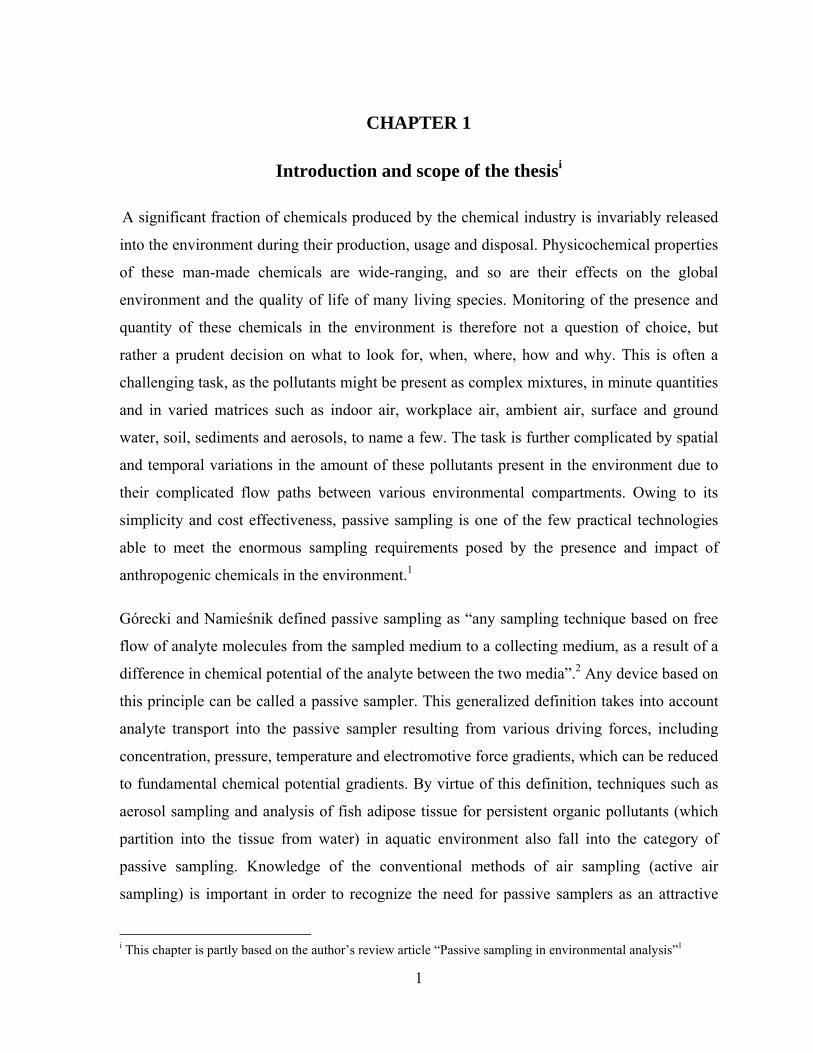
CHAPTER 1

Introduction and scope of the thesisi

A significant fraction of chemicals produced by the chemical industry is invariably released

into the environment during their production, usage and disposal. Physicochemical properties

of these man-made chemicals are wide-ranging, and so are their effects on the global

environment and the quality of life of many living species. Monitoring of the presence and

quantity of these chemicals in the environment is therefore not a question of choice, but

rather a prudent decision on what to look for, when, where, how and why. This is often a

challenging task, as the pollutants might be present as complex mixtures, in minute quantities

and in varied matrices such as indoor air, workplace air, ambient air, surface and ground

water, soil, sediments and aerosols, to name a few. The task is further complicated by spatial

and temporal variations in the amount of these pollutants present in the environment due to

their complicated flow paths between various environmental compartments. Owing to its

simplicity and cost effectiveness, passive sampling is one of the few practical technologies

able to meet the enormous sampling requirements posed by the presence and impact of

anthropogenic chemicals in the environment.1

Górecki and Namieśnik defined passive sampling as “any sampling technique based on free

flow of analyte molecules from the sampled medium to a collecting medium, as a result of a

difference in chemical potential of the analyte between the two media”.2 Any device based on

this principle can be called a passive sampler. This generalized definition takes into account

analyte transport into the passive sampler resulting from various driving forces, including

concentration, pressure, temperature and electromotive force gradients, which can be reduced

to fundamental chemical potential gradients. By virtue of this definition, techniques such as

aerosol sampling and analysis of fish adipose tissue for persistent organic pollutants (which

partition into the tissue from water) in aquatic environment also fall into the category of

passive sampling. Knowledge of the conventional methods of air sampling (active air

sampling) is important in order to recognize the need for passive samplers as an attractive

i This chapter is partly based on the author’s review article “Passive sampling in environmental analysis”1

2

alternative. Therefore, a brief discussion of active sampling methods will be presented here

before the discussion of the passive sampling technology.

1.1 Active air sampling

Since the focus of this thesis is on the quantification of Volatile Organic Compounds (VOCs)

in air, only the active sampling methods for their sampling and analysis will be discussed

here. Many definitions of VOCs have been adopted by different regulatory authorities. In this

thesis, the definition according to directive 2004/42/EC of the European Parliament will be

adopted because of its broad nature. The definition according to the Directive is the

following: “Volatile Organic Compound means any organic compound having an initial

boiling point less than or equal to 250 °C measured at a standard pressure of 101.3 kPa”.3

Active air sampling methods involve collection of contaminants onto a sampling medium by

means of a pump. The sampling medium can be an empty container, solid sorbent packed in

an inert tube, or liquid enclosed in an impinger. In the case of sampling with a solid sorbent

or a liquid, the sampled air is drawn through the sampling medium; the air stripped of the

contaminants is vented into the atmosphere. One such widely used method is the United

States Environmental Protection Agency (US EPA) method TO-17 (similar to National

Institute of Occupational Safety and Hygiene (NIOSH) method 1500 and Occupational

Safety and Health Administration (OSHA) method 07) illustrated in Figure 1-1.4 In this

method, sampling is done by drawing a known amount of air through a solid sorbent

contained in a deactivated glass or metal tube (often referred to as a sorption tube). The

analytes are then desorbed either by extracting them with a solvent (solvent desorption) or by

heating the sorbent (thermal desorption). Sorbents commonly used with solvent desorption

include silica gel, activated carbon-based sorbents (such as Anasorb® 747), carbon molecular

sieves (e.g. Carboxens®), and porous polymers. In the solvent desorption method, only a

small aliquot of the solvent extract can be used for gas chromatographic (GC) analysis and

quantification. The volume of the solvent aliquot that can be used depends on the sample

introduction system in the GC. In the thermal desorption method, the instrumentation allows

for a much larger fraction or even all of the analytes trapped by the sorbent to be introduced

into the chromatographic system for quantitation. Thermal desorption is therefore preferred

3

at times to improve the sensitivity of the method. Sorbents used in this method include

Tenax® TA, Chromosorb® 106, graphitised carbon, carbon molecular sieves, and multi-bed

combinations.5 The multi-bed combination is used when a single sorbent is not efficient in

trapping the entire range of VOCs in the sample matrix. While the sample collection is done

in the field, desorption and gas chromatographic analysis are usually done in the laboratory.

The concentration of the analyte in the air is determined from the amount of analyte collected

by the sorbent and the volume of air drawn into the sampler.

Figure 1-1: Schematic of EPA method TO-17

Active air sampling can also be performed by collecting the air sample in a container made of

an inert material. Samples obtained in this way are often termed “grab samples”. Depending

on the analytes of interest, the containers may be deactivated glass or metal bottles, or bags

made of Saran™, Mylar™, Teflon™ or Tedlar® polymers.6 Tedlar® is the material used

most often, and has been referenced in EPA methods 3, 18 and 40. The collected sample is

then transported to the laboratory, and the sampled air is analyzed using suitable

quantification methods. For the quantification of VOCs, gas chromatography with flame

ionization detection (FID), electron capture detection (ECD) or mass spectrometry (MS) is

most often used.

Although the final sample analysis is usually performed in the laboratory, there are often

situations, like emergencies due to chemical spillage, when real-time measurements of

analyte concentrations are needed. Some of these methods are discussed in the next section.

Air

Sorbent tube Flow meter Suction pump

Thermal desorption or

solvent desorption

Offline

Chromatography

4

1.1.1 Real-time pollutant measurement

Various analytical methods are available for real-time analysis, which are capable of

quantifying low concentrations of VOCs. They include differential optical absorption

spectroscopy (limit of detection (LOD) ~2.6 µg/m3 for benzene), low-pressure chemical

ionization/tandem mass spectrometry (MS2) (LOD ~2.0 µg/m3 for benzene), atmospheric

pressure chemical ionization/MS2 (LOD ~38.3 µg/m3 for benzene) and proton-transfer

reaction MS (LOD ~0.3 µg/m3 for benzene and toluene).7 The instruments are generally

installed in a vehicle for easy use at various locations based on the needs. US EPA’s Trace

Atmospheric Gas Analyzer (TAGA) is one such mobile laboratory which makes use of triple

quadrupole (QqQ) MS2 for real time analysis of various pollutants. In this method, the

ambient air is sampled continuously at a specific flow rate (typically 90 ml/min) and part of it

is directed into the ion source of a QqQ mass spectrometer for ionization, fragmentation,

detection and quantification. The specificity of MS2 (based on a series of ionization,

fragmentation and detection events) allows for quantification of the target analytes in real-

time.

The instruments mentioned in the above paragraph are expensive and require highly trained

personnel for their operation. Cheaper, hand held devices which can provide an estimate of

the total contaminant concentration in the vapor phase are also available. These include

photoionization detectors (PID) and flame ionization detectors (FID).

The PID is based on the ionization of chemical species in the sample using an ultraviolet

(UV) lamp, followed by detection of the ions formed. Commercially available PIDs have

lamps with specific ionization energies (e.g. 9.8, 10.6 or 11.7 eV); any chemical species that

can be ionized with the specific UV lamp used are detected by the PID.8 The ions created by

the action of the UV lamp generate a current in an external circuit. This current is used as a

measure of the concentration of the ionizable chemicals in the sample. The PID is often

calibrated based on the response of isobutylene, and the total concentration is expressed in

terms of isobutylene concentration. While these are handy instruments, they have a number

of disadvantages: PIDs cannot detect all the organic vapors in the sample, are not analyte

5

specific, and are affected by humidity and the presence of non-ionizable gases such as

methane.

Portable FIDs are based on ionization of organic compounds in a hydrogen flame followed

by quantification based on the signal generated by the resulting ions. This is similar to the

FIDs available for detection in GC. Any chemical species with a C-H bond is ionized and

detected by the FID. It is generally calibrated using a known concentration of methane, and

the total VOC concentration is expressed in terms of this calibrant. Both the FIDs and the

PIDs are capable of detecting concentrations in the range of 0.1 – 0.5 ppmV (as methane for

FID and as isobutylene for PID). Like PID, FID also has the disadvantage of not being

analyte-specific.9

The methods described in this section are just examples of the many variations of active air

sampling methods, with each variation being devised according to the sample matrix, analyte

type, sensitivity required, available resources, analysis time constraints, etc. Active sampling

has been used and perfected over the last few decades and led to numerous scientific

breakthroughs regarding volatile organic pollutants and their effects on animals and

vegetation. In spite of that, these methods have many disadvantages, the most important of

which cause researchers to look for alternative sampling techniques.

In the case of sampling systems using pumps, the pumps used to deliver the known amount

of air sample into the sorbent have to be calibrated. Also, such pumps are often noisy and

require electricity for their operation. The need for electricity, usually supplied from

batteries, introduces the requirement for frequent checking to ensure that the pump is

operating for its pre-determined period of time.

In the field of occupational exposure, the portable pumps are cumbersome for the employees

to carry around for prolonged periods of time. Even though the present day technology has

been able to miniaturize the sampling pumps, their presence has mostly been perceived as an

obtrusion in the normal work of an employee.10

Many pumps and other pieces of sampling equipment are required in order to collect large

numbers of samples simultaneously, e.g. when trying to map the contaminant source. Due to

6

the significant costs involved in procuring large amounts of equipment for sampling, the

number of samples collected in any given study is often limited by the amount of equipment

available. Also, costly equipment installed in the field is often prone to vandalism.

The biggest disadvantage of active sampling methods is their poor applicability to time

weighted average concentration (TWA) determination. TWA is defined as the average

concentration of a pollutant over a particular period of time. Active sampling can provide

data only on pollutant concentrations present during the short period of sampling, typically

not exceeding 24 hours. For longer time periods, active sampling requires many discrete

measurements to provide TWA concentration. Because of all the disadvantages of active air

sampling methods, passive sampling is used widely today for many applications.

1.2 Passive sampling

Since the first demonstration of truly quantitative passive sampling by Palmes and Gunnison

in 1973,11 numerous scientific peer-reviewed articles have been published on this topic.

Passive samplers were initially designed for gaseous pollutants in air, followed by their

application to aqueous matrices, and, more recently, solid matrices such as soils and

sediments. According to the definition of Górecki and Namieśnik presented earlier, air

sampling using evacuated containers such as SUMMA™ canisters can also be classified as

passive sampling. The discussion of the passive sampling technique in this section does not

apply to SUMMA™ canisters (they are covered in detail in section 1.5.1).

As an analytical chemistry tool, passive sampling is used to achieve some or most of the

basic sample preparation goals. These include among others isolation of the analytes from the

matrix and their pre-concentration to increase the selectivity and sensitivity of the

measurements, chemically changing the analyte to a form suitable for the analytical

measurement, and/or reduction of, or complete elimination of solvent use (green chemistry).

With most passive samplers, reduction and/or elimination of matrix interferences can be

easily achieved, although new matrix components might be introduced with certain passive

samplers, prompting the need for further sample clean-up.

7

Passive sampling has many practical advantages, including cost effectiveness, little training

required to handle the devices, and no need for power sources for their operation.

Furthermore, it is often useful to be able to determine TWA concentrations. Many passive

samplers can easily provide TWA concentrations, which is difficult (though not impossible)

to obtain with active/grab sampling technologies, as explained above.

Many passive samplers are available commercially or from various research groups today.

Factors affecting the design of these samplers include:

i. The sampled medium, or the matrix (air, water, soil, or various combinations of these,

such as sediments or aerosols);

ii. Chemical and physico-chemical properties of the analyte(s) of interest;

iii. Analyte form (ionized, non-ionized, sorbed, etc.) and concentration range in the sample;

iv. Quantitative or semi-quantitative type of measurement required;

v. Sampling duration required (e.g. 8 hr workplace exposure vs. several weeks exposure in

environmental monitoring);

vi. Variability of environmental parameters around the sampler or in the sample in which

the samplers are to be deployed;

vii. Cost and availability.

Since a number of variables have to be considered, there are situations where combinations

of passive samplers have to be deployed to obtain the data required. While the physical

deployment of passive samplers is fairly simple, the sampling strategy involved in choosing

the number and type of passive samplers for deployment, their exact locations, time and

duration of exposure, as well as quantification in the laboratory, require careful

consideration. The knowledge of the pollution source, quantity and potential fate in the

environment, as well as of the analytical methods used for quantification, are required for

proper data interpretation.

The sampler presented in this thesis was developed for the analysis of VOCs in the vapor

phase, with main applications including indoor/outdoor air and soil-gas analysis. In the

following sections, the principle of operation of passive sampling devices will be explained,

followed by a review of a selection of currently available passive samplers and their designs.

8

The knowledge of the effect of various environmental parameters on different types of

samplers is very important, hence this aspect will be discussed next. While proposing a

design/model for a passive sampler to be applicable for routine use, it is important to

understand and consider the regulatory requirements put forward by various agencies as

applied to the validation of the passive sampling technology. Consequently, a summary of

the relevant regulatory documents will be presented. The scope of the thesis will then be

defined and listed.

1.3 General principles of operation

Even though many different designs of passive samplers are available on the market today,

nearly all of them (with some exceptions, like the SUMMA™ canisters) consist of a barrier

and a sorbent, the material and geometry of which are carefully chosen for the specific type

of analyte and matrix. The barrier is generally one of two types: a static layer of air

(diffusion-type samplers) or a polymer membrane (permeation-type samplers), as depicted in

Figure 1-2. Within the barrier, convective transport of analytes is preferentially avoided, so

that the net transport across it occurs mainly due to molecular diffusion following Fick’s

laws. For the sake of clarity, “barriers” in this thesis will not include the boundary layers (see

later). The function of the sorbent is to adsorb or absorb analyte molecules reaching its

interface with the barrier. Chemical reaction between the analyte and the sorbent can also be

used to trap the analytes; the phenomenon is referred to as chemisorption. Adsorption is a

surface phenomenon in which a chemical species (an adsorbate) associates with the surface

of the material (adsorbent) due to intermolecular forces acting between the two. Absorption

is a process in which a substance (an absorbent, usually a liquid) takes up (or dissolves) a

chemical species (absorbate) uniformly within its matrix. Adsorbents, absorbents and

chemically reacting materials are collectively referred to as “sorbents” in this thesis. Sorbents

in various passive samplers are described later in the review.

9

Figure 1-2: Conceptual design of a passive sampler

When a passive sampler of such a design is exposed to the sample matrix, analyte molecules

are transferred into the sampler spontaneously under a concentration or partial pressure

gradient existing between the barrier-sample matrix interface and the sorbent-barrier

interface. The function of the sorbent is to completely absorb (or adsorb) all the analyte

molecules reaching the interface between the sorbent and the barrier of the sampler so that

the concentration at this interface is practically zero. Under such conditions, the kinetics of

analyte transfer to the sorbent in a given period of time obey Fick’s laws of molecular

diffusion. Consequently, analyte concentration in the sample matrix can be calculated from

the measured mass of the analyte present in the sorbent.

Analyte collection by the sorption material begins when the sampler is exposed to the sample

matrix. The uptake of the analyte into the sampler can be generally represented by a one-

compartment model shown in Figure 1-3.12 According to the model, analyte uptake proceeds

until the chemical potentials of the analyte in the sorbent and in the sample matrix become

equal. Depending on the barrier type, the sorption material, the sampler geometry and the

sampling duration, a passive sampler can function in the following three regions (Figure 1-3):

the kinetic region, the equilibrium region, or the intermediate region. In the kinetic region,

the sorbent is far from saturation (or equilibration) and therefore any molecule arriving at its

Sample matrix-barrier interface

Barrier-sorbent interface

Static layer of air (diffusive sampling) or

polymer membrane (permeation sampling)

Sorbent Analyte

movement

Barrier

10

surface is effectively trapped. The analyte amount collected by the sampler is then directly

proportional to the time period for which the sampler is exposed to the sample medium.

Within the equilibrium region, either the active sites are all blocked (adsorbents) or

equilibrium has been reached (absorbents). In this case, the analyte amount collected by the

sampler is independent of the exposure time. Between the kinetic and the equilibrium region,

the analyte uptake is non-linear, hence this region is seldom used for quantitative purposes.

Figure 1-3: Analyte uptake as a function of time (based on ref. 12)

1.3.1 Passive air sampling

When sampling from air, a sorbent is often chosen that acts as a zero sink (i.e. analyte

concentration at the sorbent-barrier interface is practically zero), which implies that the

sampler functions in the kinetic region making TWA concentration determination

straightforward. This is often accomplished by using adsorption or chemisorption-based

sorbents. When adsorption-based sorbents are used, care must be taken to allow only for low

mass loadings to minimize competitive adsorption processes, which become pronounced

under high mass loading conditions.

Based on the conceptual design shown in Figure 1-2, various samplers of different geometry

and materials are made depending on the type of application. Figure 1-4 illustrates a so-

Time

Kinetic region Equilibrium region

Ana

lyte

mas

s upt

ake

11

called “tube-type” sampler, while Figure 1-5 illustrates a “badge-type” sampler. The latter

uses either a semi-permeable membrane, or a porous material (such as ceramic) as the uptake

rate-limiting barrier.

Figure 1-4: Tube-type passive sampler

Figure 1-5: Badge-type passive sampler

The sampler used in this project is of permeation-type, resembling the badge-type sampler

shown in Figure 1-5. When sampling under the kinetic region illustrated in Figure 1-3, ideal

concentration profiles for analyte uptake from air by the diffusion- and permeation-type

passive samplers are illustrated in Figures 1-6 and 1-7, respectively.13 In the case of

diffusion-type samplers, the analyte concentration within the barrier varies from a maximum

Sample matrix Sorbent

Static layer of air

Molecular diffusion path

Semi-permeable membrane/ porous material.

Sorbent

Analyte molecules

Sample matrix

12

corresponding to the analyte concentration in the air to zero at the sorbent-barrier interface.

In the case of permeation-type samplers, analyte transfer from the sample into the sorbent in

the sampler (through the polymer membrane) involves three steps: dissolution of the vapor

molecules in the polymer (determined by the partition coefficient of the analyte between air

and the membrane material), diffusion of the molecules through the membrane material

under a concentration gradient, and the release of the vapor from the polymer at the opposite

side of the membrane.14 The concentration of the analyte on the surface of the membrane

exposed to the sample depends on its concentration in air and its partition coefficient between

air and the membrane material. For polydimethylsiloxane (PDMS) membrane barriers,

partition coefficients of VOCs are typically much greater than one (examples of partition

coefficients of n-alkanes are provided in Chapter 2). The concentration of VOCs on the

membrane surface on the sample side is therefore much higher than the concentration in the

air. The relationships between analyte concentration in the air, sampler geometry, time of

exposure and mass uptake into the sampler are summarized for the two types of samplers in

Table 1-1.15,16

Analyte concentration in

air

“Zero sink” sorbent

Diffusion path

Sample

Distance

Con

cent

ratio

n

Figure 1-6: Ideal concentration profile for diffusion-type passive samplers (based on ref. 13)

13

Figure 1-7: Ideal concentration profile for permeation-type passive samplers (based on ref.

13)

Table 1-1: Fick’s law as applied to diffusive- and permeation-type passive samplers (based

on refs. 15 and 16) Diffusion sampler Permeation sampler

Application of Fick’s law

( )CCLAD

tM

d

−=⎟⎠⎞

⎜⎝⎛

0

D - Diffusion coefficient of the analyte A - Area of the cross-section of the diffusion barrier Ld - Length of the diffusion path C - Concentration of the analyte near the diffusion path- sorbent interface C0 - Concentration of the analyte in the vicinity of the diffusion barrier inlet

( )msmam

CCLAD

tM

−=⎟⎠⎞

⎜⎝⎛

D - Diffusion coefficient of the analyte in the membrane A - Surface area of the membrane Lm - Membrane thickness Cma concentration of the analyte on the surface of the membrane exposed to air

oma KCC = K - Partition coefficient of the analyte between the air and the membrane C0 - Concentration of the analyte in air near the external membrane surface Cms - concentration of the analyte on the membrane surface in contact with the sorbent.

Definition of the calibration constant k AD

Lk d= DKAL

k m=

TWA concentration determination t

kMC =0 t

kMC =0


air

Analyte concentration at the surface of the

membrane“Zero sink”

sorbent

Sample

Membrane thickness

Distance

Con

cent

ratio

n

14

1.3.2 Passive water sampling

When sampling from aquatic environments, the barriers are usually made of polymers such

as polyethylene, PDMS, polysulfone, regenerated cellulose, silicone-polycarbonate, cellulose

acetate, polytetrafluoroethylene (PTFE), nylon, polypropylene, polyvinyl chloride, etc. The

polymeric membranes form a physical barrier to water molecules. Porous materials are also

used as barriers, in which case analyte transfer is controlled by diffusion through water in the

pores or through air trapped in the pores. In contrast to air sampling, where adsorption-based

sorbents are most often used, water sampling usually involves samplers with sorbents that

trap analytes via partitioning. In such cases, the sorption material is not a zero sink, and the

analytes can reach equilibrium within a few minutes to several weeks depending on the

amount and sorption capacity of the sorbent used.

The passive sampler developed in this project is for application in air and soil-gas analysis;

consequently, a review focused only on passive sampling technologies currently available for

these two matrices will be presented here.

1.4 Literature review

The reviews related to passive sampling technology published over the last three-and-a-half

decades make it possible to follow its development with relative ease (Table 1-2).

Immediately after its introduction, the technology was primarily adopted for workplace

exposure measurements; the first notable review of such application was perhaps the one by

Saunders, published as early as 1981.17 By 1984, samplers such as PRO-TEK (DuPont),

Palmes (MDA), VaporGard (MSA), GASBADGE (National Mine Safety), and 3M’s

mercury, organic and carbon dioxide monitors had appeared on the market. In 1986, an

international symposium was held in Luxemburg on diffusive sampling with emphasis on

workplace air monitoring, which resulted in the publication of one of the most

comprehensive literature collections on diffusive sampling at that time in the following

year.18 Even though the first passive sampler for waterborne pollutants was patented as early

as 1980 by Aylott and Byrne,19 the technology growth was slow until Södergren developed

and reported the in-situ mimetic passive sampling device in 1987.20 By 2000, several such

samplers were being used all over the world. Górecki and Namieśnik reviewed the status of

15

the technology in 2002. This review included the passive sampler’s applications in air, water

and soil matrices, and by virtue of the definition adopted (stated earlier) it also included bio-

monitoring as a type of passive sampling based on accumulation of organic pollutants in the

tissue of living organisms. The number of books dedicated specifically to passive sampling

techniques is small, though many general air sampling-related publications include a section

on this technology. Brown et al. compiled books containing the proceedings of international

symposia held in Luxembourg in 1990.21 A book authored by Huckins et al. provided a

comprehensive treatment on semipermeable membrane devices (SPMDs).22 A general

treatise on passive sampling for environmental applications by Greenwood et al. is a recent

addition to the list of available books.23

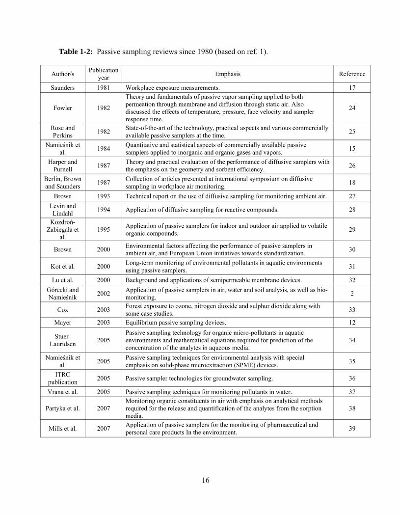
16

Table 1-2: Passive sampling reviews since 1980 (based on ref. 1).

Author/s Publication year Emphasis Reference

Saunders 1981 Workplace exposure measurements. 17

Fowler 1982

Theory and fundamentals of passive vapor sampling applied to both permeation through membrane and diffusion through static air. Also discussed the effects of temperature, pressure, face velocity and sampler response time.

24

Rose and Perkins 1982 State-of-the-art of the technology, practical aspects and various commercially

available passive samplers at the time. 25

Namieśnik et al. 1984 Quantitative and statistical aspects of commercially available passive

samplers applied to inorganic and organic gases and vapors. 15

Harper and Purnell 1987 Theory and practical evaluation of the performance of diffusive samplers with

the emphasis on the geometry and sorbent efficiency. 26

Berlin, Brown and Saunders 1987 Collection of articles presented at international symposium on diffusive

sampling in workplace air monitoring. 18

Brown 1993 Technical report on the use of diffusive sampling for monitoring ambient air. 27 Levin and Lindahl 1994 Application of diffusive sampling for reactive compounds. 28

Kozdroń-Zabiegała et

al. 1995 Application of passive samplers for indoor and outdoor air applied to volatile

organic compounds. 29

Brown 2000 Environmental factors affecting the performance of passive samplers in ambient air, and European Union initiatives towards standardization. 30

Kot et al. 2000 Long-term monitoring of environmental pollutants in aquatic environments using passive samplers. 31

Lu et al. 2000 Background and applications of semipermeable membrane devices. 32 Górecki and Namieśnik 2002 Application of passive samplers in air, water and soil analysis, as well as bio-

monitoring. 2

Cox 2003 Forest exposure to ozone, nitrogen dioxide and sulphur dioxide along with some case studies. 33

Mayer 2003 Equilibrium passive sampling devices. 12

Stuer-Lauridsen 2005

Passive sampling technology for organic micro-pollutants in aquatic environments and mathematical equations required for prediction of the concentration of the analytes in aqueous media.

34

Namieśnik et al. 2005 Passive sampling techniques for environmental analysis with special

emphasis on solid-phase microextraction (SPME) devices. 35

ITRC publication 2005 Passive sampler technologies for groundwater sampling. 36

Vrana et al. 2005 Passive sampling techniques for monitoring pollutants in water. 37

Partyka et al. 2007 Monitoring organic constituents in air with emphasis on analytical methods required for the release and quantification of the analytes from the sorption media.

38

Mills et al. 2007 Application of passive samplers for the monitoring of pharmaceutical and personal care products In the environment. 39

17

1.5 Passive air samplers

A number of passive samplers are available for sampling VOCs from air. Selected passive

samplers, representative of the different designs, materials of construction and analytes, are

summarized here. Among the passive samplers discussed, the SUMMA™ canisters and

3M™ OVM samplers were used in this project and will be also dealt with in Chapters 6 and

7.

1.5.1 SUMMA™ canisters

Sampling of VOCs from air with SUMMA™ canisters has been widely employed and is

generally considered and marketed as a passive sampling technique. Examples of validated

air sampling methods using SUMMA™ canisters include EPA methodsTO-14A40 and TO-

15.41 These canisters are specially designed and deactivated using a proprietary passivation

technique called the “SUMMA” process, in which a series of chemical deactivation and

electropolishing steps render the inner surface of the canisters chemically inert. The canisters

are available in spherical or cylindrical shapes, and with volumes typically between 1 L and 6

L.

A schematic of the sample collection and analysis method using a SUMMA™ canister is

illustrated in Figure 1-8.42 The canister is first evacuated, typically to <0.05 mm Hg, and the

canister inlet is opened to allow the sample air to flow into the canister by virtue of the

differential pressure.41 SUMMA™ canisters can be used to collect grab samples, with a

typical duration of 10 to 30 seconds, or time weighted average samples of typically 1 to 24

hour duration by using a flow-controlled inlet attached to the canister. Generally, either a

mass flow controller or a critical orifice flow controller are used for this purpose. With a

critical orifice for controlling the flow, a reduction in the flow rate occurs as the pressure

inside the canister approaches atmospheric pressure. On the other hand, the flow rate can be

maintained constant throughout the sampling period using mass flow controllers. An

interesting improvement was successfully tested and reported in 2005 by Rossner and

Ferrant.43 They used the same principle, but with a flow rate of 0.05 mL/min to collect

samples for periods from one week to several weeks long using a 6 liter SUMMA canister,

making it possible to obtain TWA concentrations for longer periods of time than achieved

18

earlier by canister methods. However this technique is not commercialized or used widely by

field personnel.

Figure 1-8: Schematic of EPA method TO-14 A and 15

Once the sample is collected in the canister, it is transported to the laboratory for analysis.

Owing to inertness of the inner walls of the canisters, the samples can generally be stored in

them for 14 to 30 days prior to the analysis without any significant decrease in analyte

recovery. In the laboratory, the pressure in the canister is increased using zero-grade nitrogen

as the diluent gas. After equilibration, this elevated pressure allows measured aliquots of the

sample gas to be easily withdrawn for analysis. Analyte collection and pre-concentration

from the diluted air sample in the canister is achieved through collection on thermally

desorbable sorbent tubes or by using cryogenic techniques, followed by thermal desorption

and gas chromatography. Method TO-14A utilizes chromatographic analysis with ECD or

FID detectors, while method TO-15 utilizes chromatography combined with MS. Analyte

concentrations in the range of parts per billion by volume can be easily determined using this

method. The concentration of the analytes in the sampled air is then calculated based on the

Analyte trapping with cryogen

or solid sorbent

Air

Thermal desorption Chromatography

Offline

19

initial pressure inside the canister before sampling, final pressure after sampling, and canister

pressure after pressurization with zero grade nitrogen.

Analytical results obtained using SUMMA™ canisters are legally defensible and hence are

routinely used for ambient air and indoor air applications where risk assessment is involved.

Canisters have also found widespread use in soil gas sampling and analysis required for

vapor intrusion monitoring. Such applications will be discussed in Chapters 6 and 7.

Even though SUMMA™ canisters have been found to be applicable to many areas, they have

several significant disadvantages. Canister deployment, sample processing and analysis are

more cumbersome with SUMMA™ canisters compared to most other passive samplers. The

cost is relatively high (~$250 to $ 400$ per sample) as it includes canister rental, cleaning

and certification, flow controller rental and cost of analysis. Further, the canisters are often

considered obtrusive by occupants when used for indoor air sampling. Obtaining long term

TWA concentration data (from 1 day to several weeks) from one canister is not currently

possible with the commercially available SUMMA™ canisters.

1.5.2 3M™ Organic Vapor Monitor (OVM) 3500 sampler

OVM 3500 (Figure 1-9) is a diffusive-type passive sampler marketed by 3M Inc. (St. Paul,

MN). Activated carbon-based material (160 mg), pressed to form a disc, is used as the

sorbent in this sampler.44 A thin microporous PTFE membrane (pore size 0.1 µm) serves as a

wind screen.45 The PTFE membrane and the sorbent disc are 1 cm apart, which defines the

diffusion path for the analyte transport from the sample matrix to the sorbent. The cross-

section area for diffusion is large at 7.07 cm2. Once the sampling is completed, the sorbent is

removed from the sampler and extracted with CS2, followed by chromatographic analysis of

the extract for quantification. Analyte uptake rate needs to be sufficiently high in order to

sample enough analytes for quantification when the concentration is close to the regulatory

limits. Because of the large cross section area and relatively short diffusion path length of the

OVM samplers, the analyte uptake rates are high enough for use in routine 8 hour workplace

exposure monitoring.

20

Figure 1-9: 3M™ OVM 3500 sampler (reproduced from ref. 46)

1.5.3 Solid-phase microextraction device

SPME device consists of a short fused silica fibre which is coated with an extracting phase

(typically 1 cm long and 0.11 mm outer diameter).47 The coated fibre is housed inside a

stainless steel needle in such a way that it can be moved in and out of the needle for exposing

the extraction phase to the sample matrix, as well as for introducing the fibre into a GC

injector for thermal desorption and quantification of the extracted analytes. When the

extraction phase is exposed to the sample matrix, the analytes are either adsorbed or

absorbed, and the analyte uptake follows the profile as illustrated in Figure 1-3. The sampler

is generally exposed for sufficient time for the analyte to equilibrate between the sampler and

the extraction phase. The time to reach equilibrium is often on the order of a few minutes.

Once the extraction is complete, the fibre is retracted into the stainless steel needle and then

introduced into a GC injector using the needle as a guide. When the needle is in the injector,

the fibre is exposed to the carrier gas flowing through the hot injector, which causes analyte

desorption. The gas then carries the analytes into the GC column for separation and

quantification. When the sample volume is large compared to the volume of the extraction

phase, the amount of analyte (n) collected by the fibre at equilibrium is given by:

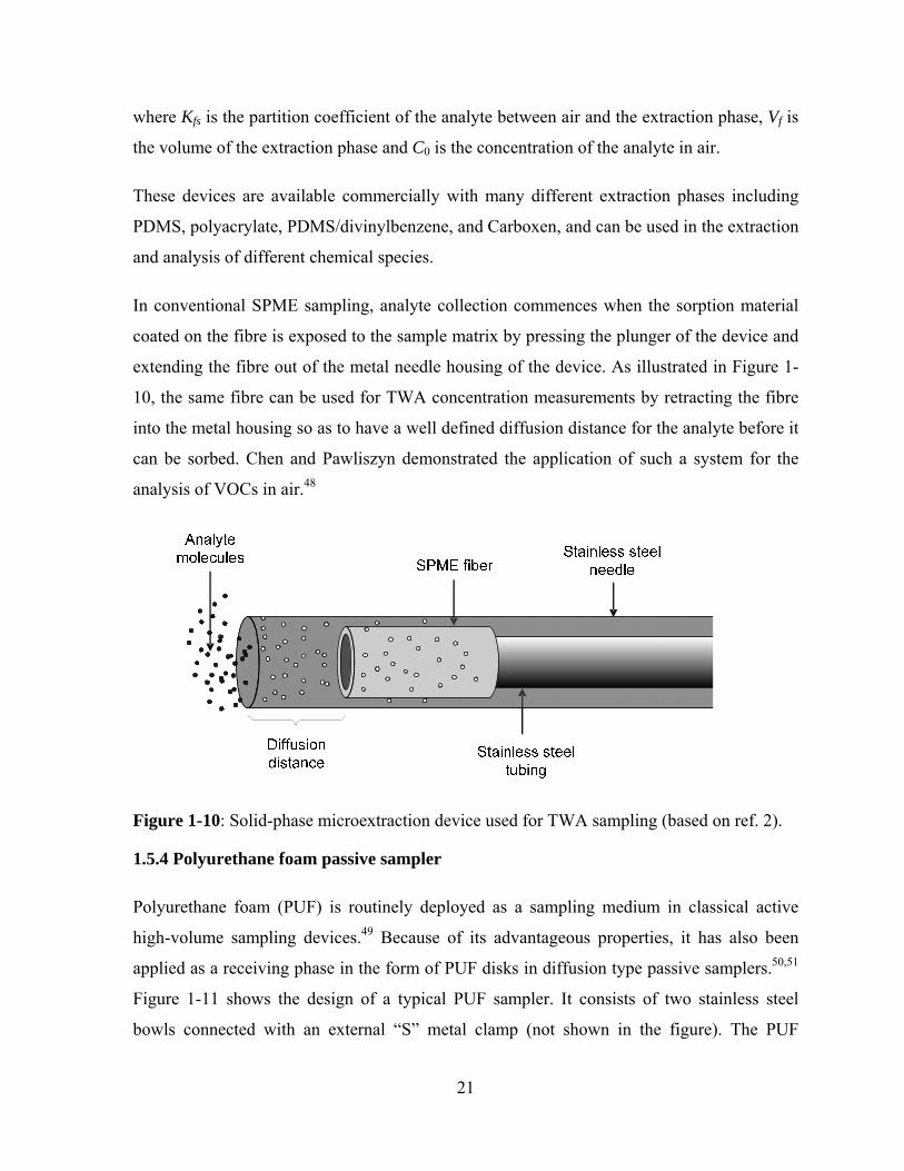
21

where Kfs is the partition coefficient of the analyte between air and the extraction phase, Vf is

the volume of the extraction phase and C0 is the concentration of the analyte in air.

These devices are available commercially with many different extraction phases including

PDMS, polyacrylate, PDMS/divinylbenzene, and Carboxen, and can be used in the extraction

and analysis of different chemical species.

In conventional SPME sampling, analyte collection commences when the sorption material

coated on the fibre is exposed to the sample matrix by pressing the plunger of the device and

extending the fibre out of the metal needle housing of the device. As illustrated in Figure 1-

10, the same fibre can be used for TWA concentration measurements by retracting the fibre

into the metal housing so as to have a well defined diffusion distance for the analyte before it

can be sorbed. Chen and Pawliszyn demonstrated the application of such a system for the

analysis of VOCs in air.48

Figure 1-10: Solid-phase microextraction device used for TWA sampling (based on ref. 2).

1.5.4 Polyurethane foam passive sampler

Polyurethane foam (PUF) is routinely deployed as a sampling medium in classical active

high-volume sampling devices.49 Because of its advantageous properties, it has also been

applied as a receiving phase in the form of PUF disks in diffusion type passive samplers.50,51

Figure 1-11 shows the design of a typical PUF sampler. It consists of two stainless steel

bowls connected with an external “S” metal clamp (not shown in the figure). The PUF

22

sorbent is placed in the bottom bowl with the help of a stainless steel support. The space

between the two bowls and the openings in the bottom bowl provide air and analyte

movement in and out of the arrangement. Shoeib et al. applied PUF disk passive samplers in

the collection of perfluoroalkyl sulfonamides in indoor and outdoor air. The PUF disks (14

cm diameter, 1.35 cm thick) were suspended in a special chamber to prevent the deposition

of coarse particles, as well as to eliminate ultraviolet radiation and minimize the effect of

wind speed on the uptake in the case of outdoor applications. Because PUF has a high

retention capacity for persistent organic pollutants (POPs) which are delivered by air

movement, PUF disk passive samplers were applied by Shoeib et al. for the analysis of

airborne POPs in Canada and Chile.50,52,53 PUF disk passive samplers were also applied for

the determination of PCBs across Europe.54 Other examples include application of PUF

passive samplers for polychlorinated naphthalenes (PCNs) and toxaphene,55 polybrominated

diphenyl ethers (PBDEs) and PCBs.56

Figure 1-11: Design of a polyurethane foam diffusive sampler (based on ref. 57)

1.5.5 Other air samplers reported in literature

As depicted in Figures 1-2 and 1-3, passive samplers are composed of a barrier and a sorbent,

and generally operate either in the kinetic or the equilibrium region. Table 1-3 provide details

on various passive samplers used for sampling from air with these parameters in context, as

well as information on the analytes for which specific passive samplers can be used.

23

Table 1-3: Diffusion/permeation barriers and receiving phases used in various passive samplers for the application in air (based on ref. 1).

Air sampling Barrier type Sorbent/receiving phase Operation region Analyte type References

SUMMA canisters None (flow regulated by various flow controlling devices) None (electro-polished, evacuated canister) Equilibrium VOCs 41

Tristearin-coated fibreglass sheets None Tristearin on fibreglass cloth Equilibrium SVOCs 58

Polymer coated glass (POG) None (sometimes partially enclosed in a stainless steel bowl)

Ethylene vinyl acetate (EVA) coated on a glass cylinder Equilibrium Persistent organic

pollutants 59,60,61

Polyethylene-based passive sampling devices (PSD) None Low density polyethylene Equilibrium PAHs 62

XAD-2 resin-based sampler None (stainless steel shelter) XAD-2 resin (styrene-divinylbenzene) Kinetic Persistent organic pollutants 63

Palmes tube Diffusion through static air in a tube Stainless steel mesh impregnated with triethanolamine Kinetic NO, NO2, SO2 11,33,64

Reiszner-West badge Permeation through silicone membrane Sodium tetrachloromercurate Kinetic SO2, CO 65,66,67,68

Willems badge Diffusion through microporous PTFE and air Citric acid, NaI/NaOH, Kinetic NH3,NO2 33,69,70

Developed by Yanigasawa-Nishimura Diffusion through perforated polypropylene Cellulose fibre filter paper containing

triethanolamine Kinetic NO2 and NO 71

OVM 3500,3520 (3M) Diffusion through static air Single or double adsorbent depending on the analyte(s) Kinetic VOCs 72,73,74

Perkin-Elmer tubes Diffusion through static air in the tube Various thermally desorbable sorbents depending on analytes Kinetic VOCs 75,76

Ogawa sampler Diffusion through air channels in plastic material. Various pre-coated collection pads Kinetic NH3,NOx,SO2, O3 77,78,79

Ferm Dosimeter Badge-type, diffusion through air and with wind-shielded inlet

Impregnated filter, various chemicals depending on analyte Kinetic NH3,NO2,SO2 80,81,82,83

TOPAS (Combined with thermal

desorption system of Gerstel) Diffusion through microporous PTFE Tenax/Thermal desorption Kinetic VOCs (not suitable for

highly polar compounds) 84

ORSA-5 (Dräeger) Diffusion through static air in a tube on either side of the sorbent Activated charcoal/solvent desorption Kinetic VOCs 85,86,87

24

Table 1-3 (continued): Diffusion/permeation barriers and receiving phases used in various passive samplers for the application in air (based on ref. 1).

Air sampling Barrier type Sorbent/receiving phase Operation region Analyte type References

PRO-TEK, G-AA/G-BB (Dupont)

Diffusion through perforated plastic placed on either side of the sorbent strip Activated carbon strip/solvent desorption Kinetic Most organic vapors 88,89

Analyst Diffusion through stainless steel mesh and air cavity in the badge

Granular activated charcoal/solvent desorption Kinetic VOCs 90,91

Radiello Diffusion through microporous polyethylene film and air

Carbograph 4 thermal desorption Kinetic VOCs 91,92

Gas Adsorbent Badges for Individual Exposure (GABIE)

sampler

Diffusion through porous PUF windscreen and static air.

Activated carbon solvent desorption Kinetic VOCs 91,93

SKC 575 series of samplers Diffusion through channels in plastic body (badge-type).

Activated charcoal, Anasorb 747®, Anasorb 727®

solvent desorption Kinetic VOCs 94,95,96

SKC 590 series of samplers Diffusion through channels in plastic body (badge-type).

Tenax, Carbopack-X thermal desorption Kinetic VOCs 97

Shibata gas-tube sampler Porous PTFE tube Granular activated carbon Kinetic VOCs 98

Namieśnik et al. Permeation through PDMS membrane Activated carbon Kinetic VOCs 99,100 Sep-pak Xposure DNPH

cartridge Diffusion through porous polyethylene filter and static

air 2,4-dinitrophenylhydrazine-coated silica

cartridge (Waters Sep-Pak XpoSure) Kinetic Selected aldehydes and ketones 101

GMD sampler (UMEx – 100) Diffusion through channels drilled into polypropylene plate

Papers impregnated with various reagents for different analytes Kinetic Aldehydes, amines

etc.

101,102,103

Seethapathy and Górecki Permeation through PDMS Activated carbon-based sorbents solvent desorption Kinetic VOCs 104

PUF sampler Diffusion through air Polyurethane foam (enclosed between stainless steel bowls) Kinetic VOCs and SVOCs 49,50,51,52,53,54,55,56,

105, 106, 107

Designed by Yamamoto et al. Porous PTFE membrane (0.1 μm pore size) Carbopack B (60-80 mesh) Kinetic VOCs 45

SPME Diffusion through static air (SPME fibre retracted into the needle) Various sorbents Kinetic VOCs 48

SPMD Low density polyethylene. Historically, silicone,

polypropylene and polyvinyl chloride have also been tried

Triolein Kinetic, non

linear, equilibrium

Non-polar hydrophobic compounds

22

25

1.6 Passive soil gas sampling

Compared to passive sampling techniques applied to air and aqueous matrices, the

application to solid matrices (such as soil, sediment, and compost) has a relatively short

history. Concentration of chemical species in soil gas is dependent on many variables, such

as soil particle size and mineralogy, organic and moisture contents, temperature and overall

heterogeneity of particle size and composition. As a result, most passive soil gas sampling

applications are restricted to qualitative or screening purposes only, and few provide truly

quantitative data. Sample spacing, sample collection depth, exposure period, etc., are key

factors for both passive and active approaches. A detailed description of these factors has

been provided by Morrison.108 An adoption of these concepts can be found in a site

assessment manual used in the USA.109

Passive soil gas samplers have been used for many purposes, including pollutant monitoring,

soil gas/vapor survey in site assessment, evaluation of soil remediation performance,

underground pipeline leak detection, soil/rock radiation detection, petroleum resource

exploration, as well as soil fertility surveys.110,111. In these applications, sampling and

measurement of chemicals of all kinds, such as VOCs, semi-volatile organic compounds

(SVOCs), petrochemicals, non-aqueous-phase liquids (NAPL), pesticides, radon gas,

explosives, carbon monoxide and nitrogen dioxide have been reported. Currently, GORE™

Module, PETREX sampler, SPMD, solid phase microextraction (SPME) and selected other

samplers are used for soil gas sampling. A brief description and application of these soil gas

sampling systems is provided in the following sections.

1.6.1 GORE™ modules

Since they were patented in 1992, GORE™ modules have been widely used for air, water

and soil gas sampling applications.23 These modules make use of expanded

polytetrafluoroethylene (GORE-TEX®) membrane as the barrier material, and various

proprietary polymeric and carbonaceous resin mixtures as adsorbents. The adsorbents are

capable of trapping a wide variety of organic compounds including VOCs and SVOCs

ranging from ethane (C2) to phytane (C20). The sorbent is enclosed by the GORE-TEX®

26

membrane and takes a flexible tubular form to which a support chord (also made of GORE-

TEX®) is attached for installation and retrieval purposes. Because of the high surface tension

of water and hydrophobic nature of the GORE-TEX membrane (with pore size of 0.2 µm),

liquid water does not cross the membrane.112 However, the membrane still allows water

vapor to diffuse through it. The GORE-TEX™ membrane also protects the adsorbent from

soil particles, enabling sensitive soil gas sampling. The GORE™ modules are generally

installed inside 1-2 cm diameter holes drilled into the ground to a depth of typically 50-100

cm. After deployment, exposure and retrieval, the modules are transported to the laboratory

for analysis. The modules are then analysed using thermal desorption-GC-MS.

The GORE™ module has been deployed in virtually all geological settings (from low

permeability clays to high permeability sands) at all moisture levels (from dry to saturated

soils) to detect VOCs and SVOCs. In a field test conducted by the United States

Environmental Protection Agency (US-EPA) Environmental Technology Verification (ETV)

program using GORE™ Module passive soil gas sampling system in 1997, its applicability

was demonstrated at two sites: one composed primarily of clay soil, and the other composed

primarily of medium to fine-grained sandy soil.113 The results showed that the GORE™

method could detect VOCs (including vinyl chloride, cis 1,2-dichloroethylene (cis DCE),

1,1-dichloroethane, 1,1,1-trichloroethane (1,1,1 TCA), trichloroethylene (TCE) and

tetrachloroethylene (PCE)) at lower concentrations in the subsurface than the reference active

soil gas sampling method. However, at higher concentrations, the ratio between the mass of

contaminant in soil gas detected using the GORE™ module and the concentration of

contaminant in soil gas detected using the reference soil gas sampling method decreased. The

authors suggested that sorbent saturation may have occurred at high concentrations. Monks et

al. described the use of GORE™ modules consisting of chemical-specific organic

compound-sensitive resins.114 The samplers were inserted 3 feet into the ground inside

predrilled holes for the determination of VOCs and SVOCs at a naval facility. The study

demonstrated that the GORE™ module method could be used to determine the presence of

both VOCs and SVOCs in the subsurface, whereas conventional active methods are limited

mainly to VOC screening.

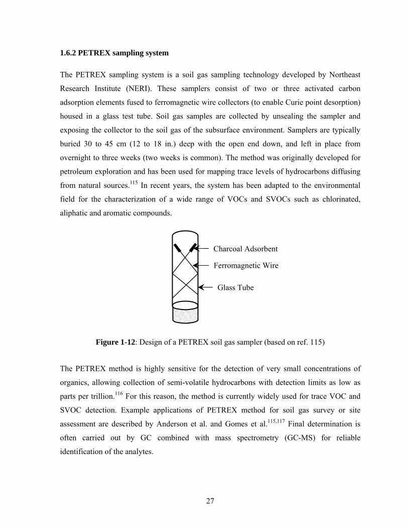
27

1.6.2 PETREX sampling system

The PETREX sampling system is a soil gas sampling technology developed by Northeast

Research Institute (NERI). These samplers consist of two or three activated carbon

adsorption elements fused to ferromagnetic wire collectors (to enable Curie point desorption)

housed in a glass test tube. Soil gas samples are collected by unsealing the sampler and

exposing the collector to the soil gas of the subsurface environment. Samplers are typically

buried 30 to 45 cm (12 to 18 in.) deep with the open end down, and left in place from

overnight to three weeks (two weeks is common). The method was originally developed for

petroleum exploration and has been used for mapping trace levels of hydrocarbons diffusing

from natural sources.115 In recent years, the system has been adapted to the environmental

field for the characterization of a wide range of VOCs and SVOCs such as chlorinated,

aliphatic and aromatic compounds.

Figure 1-12: Design of a PETREX soil gas sampler (based on ref. 115)

The PETREX method is highly sensitive for the detection of very small concentrations of

organics, allowing collection of semi-volatile hydrocarbons with detection limits as low as

parts per trillion.116 For this reason, the method is currently widely used for trace VOC and

SVOC detection. Example applications of PETREX method for soil gas survey or site

assessment are described by Anderson et al. and Gomes et al.115,117 Final determination is

often carried out by GC combined with mass spectrometry (GC-MS) for reliable

identification of the analytes.

Ferromagnetic Wire

Glass Tube

Charcoal Adsorbent

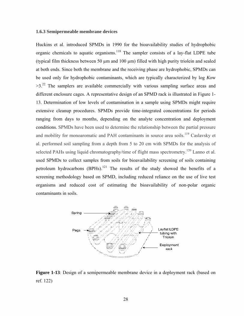
28

1.6.3 Semipermeable membrane devices

Huckins et al. introduced SPMDs in 1990 for the bioavailability studies of hydrophobic

organic chemicals to aquatic organisms.118 The sampler consists of a lay-flat LDPE tube

(typical film thickness between 50 µm and 100 µm) filled with high purity triolein and sealed

at both ends. Since both the membrane and the receiving phase are hydrophobic, SPMDs can

be used only for hydrophobic contaminants, which are typically characterized by log Kow

>3.22 The samplers are available commercially with various sampling surface areas and

different enclosure cages. A representative design of an SPMD rack is illustrated in Figure 1-

13. Determination of low levels of contamination in a sample using SPMDs might require

extensive cleanup procedures. SPMDs provide time-integrated concentrations for periods

ranging from days to months, depending on the analyte concentration and deployment

conditions. SPMDs have been used to determine the relationship between the partial pressure

and mobility for monoaromatic and PAH contaminants in source area soils.119 Caslavsky et

al. performed soil sampling from a depth from 5 to 20 cm with SPMDs for the analysis of

selected PAHs using liquid chromatography/time of flight mass spectrometry.120 Lanno et al.

used SPMDs to collect samples from soils for bioavailability screening of soils containing

petroleum hydrocarbons (BPHs).121 The results of the study showed the benefits of a

screening methodology based on SPMD, including reduced reliance on the use of live test

organisms and reduced cost of estimating the bioavailability of non-polar organic

contaminants in soils.

Figure 1-13: Design of a semipermeable membrane device in a deployment rack (based on

ref. 122)

29

1.6.4 Solid-phase microextraction

SPME technique, as discussed in Section 1.5.3, is not only widely used for air and water

sampling, but can also be applied to solid matrices.123 There are three different extraction

modes for SPME: direct, headspace and membrane,124 among which headspace SPME is the

most suitable for sampling from solid matrices. In this mode, the SPME fibre is placed in the

air directly above the soil sample contained in a vial, and analytes partition from the sample

matrix through the air to the fibre coating. The air in the vial serves as the barrier between the

SPME fibre and the sample matrix, thus preventing the fibre from potentially being

contaminated by the interferences in the sample medium. Headspace SPME was introduced

by Zhang and Pawliszyn to extend the SPME technique to more complex samples which

contain solid or high molecular weight materials, such as soil and sludge.125

1.6.5 Other samplers reported in literature

Polyethylene membrane vapor-diffusion (PVD) sampler is made from 20 or 40 mL glass

crimp-top or volatile organic analysis (VOA) vials. The empty vials are uncapped and

wrapped with two layers of low density polyethylene (LDPE) sheets.126 When the samplers

are exposed to soil gas, analyte equilibration occurs between the soil gas matrix and the air

trapped inside the vial. Once the equilibration process is complete, the samplers are capped

and returned to the laboratory for analysis. The PVD samplers were used as passive soil gas

samplers in the unsaturated zone at a petroleum tank farm for the detection of toluene.127

Based on this study, PVD samplers were found effective in the vadose zone.

EMFLUX® passive soil gas sampling system consists of a 7 mL, screw-top, glass vial with a

plastic sampling cap. The cap has a hole in it covered with a fine-mesh screen to allow for

analyte diffusion into the glass vial. A cartridge containing 100 mg of a hydrophobic,

thermally desorbable adsorbent placed inside the vial serves as the sorbent for trapping

SVOCs and VOCs in the vapor phase. A retrieval wire is connected to the sampler’s mouth

and the vial is inserted upside down into a 2 cm wide and 10 cm deep core hole drilled into

the soil matrix. The soil is then collapsed onto the sampler and the sampler is allowed to

collect analyte vapors for a predetermined amount of time. After sampling, the sampler is

removed from the soil, and the adsorbent cartridge is analyzed by thermal desorption/GC-MS

30

method. The application of EMFLUX® samplers for soil gas analysis of VOCs and SVOCs

was tested as part of the US EPA’s Environment Technology Verification Program and was

found to be applicable in clay and sandy soil matrices and provided positive identification

and semi-quantitative concentrations of target VOCs at the contaminated site.128 The

EMFLUX® sampling system has been used at mixed waste landfill,129 city schools in

Memphis,130 and sewer locations131 among others.

1.7 Effect of environmental parameters

Even though passive sampling has been widely used and recognized as a valuable tool in

environmental monitoring, the reliability of this technique under varying environmental

conditions has always been a subject of controversy. This is because the theoretical treatment

using Fick’s laws of diffusion is based on the assumption that steady-state conditions apply

to passive samplers. In reality, the concentration profile and the analyte flux across the

membrane at a particular instant during sampling is a function of many variables, including

temperature, atmospheric pressure, fluid velocity at the sampler face, sorbent effectiveness,

analyte concentration in air, humidity, etc. The potential dependence of the results on such a

large number of factors is the reason for the National Institute of Safety and Health (NIOSH)

to accept results with an accuracy of ± 25 % and a bias of ± 10 % for passive sampler

applications in air. In addition, passive samplers have to be validated by comparing their

performance with active sampling conducted in parallel. The major factors affecting these

parameters are discussed below, keeping both diffusive-type and permeation-type passive

samplers in context.

1.7.1 Temperature

Temperature plays an important role in determining the uptake rate of a sampler and is an

important factor in the validation of passive samplers. In the case of air sampling, molecular

diffusion coefficients in air increase with temperature, which results in increased uptake rates

of the analytes. The increase can be easily estimated, as the change in the rate of molecular

diffusion with temperature is well explained by the kinetic theory of gases. According to this

theory, diffusion coefficient varies as T3/2 (K) and is inversely proportional to pressure. In

practice, the uptake rate has been found to vary approximately by 0.2-0.4% per K.30

31

Nevertheless, knowledge of temperature variations is often required to apply the necessary

corrections to the uptake rate of diffusive samplers.

Temperature dependence of permeability through polymers is determined by both the

diffusion coefficient of the molecule in the polymer, and its partition coefficient between air

and the polymer. For polymers such as PDMS, the diffusion coefficient of a molecule in the

polymer increases with temperature, while the partition coefficient decreases. This trade-off

results in permeability being generally a weak function of temperature. On the other hand, for

polymers such as PTFE and polyethylene, permeability is found to increase with increasing

temperature.132,133

1.7.2 Pressure

The diffusion coefficient of molecules in air is inversely proportional to pressure, hence

pressure variations must be known accurately for accurate sampling rate corrections. While

the effect of pressure for sampling from air has been discussed,30 to the best of our

knowledge no studies have been done so far for sampling from aqueous matrices. However,

Booij et al.134 reported the use of SPMDs, low-density polyethylene (LDPE) strip samplers

and PDMS strip samplers in the sea at depths up to 5 km (hence under very high pressures)

for 1 to 1.5 years without any specific problems.

1.7.3 Face velocity

When the sampler is collecting analytes from the sample matrix, there exists a region in the

immediate vicinity of the sampler where the analyte concentration is lower than that in the

sample matrix away from the sampler. The presence of such a region of depleted analyte

concentration and its extent are both a function of the air flow pattern around the sampler.

These effects are often studied by determining the uptake rates as a function of linear flow

velocity of air across the surface of the sampler. Hori and Tanaka reported that for 3M™

OVM 3500 diffusive-type passive sampler, the uptake rate did not change from 0.5 m s-1 to

2.0 m s-1 but the uptake was substantially lower when the face velocity of air was zero.80

Such effects can theoretically be discussed based on the concept of boundary layer effect,

which is presented in detail in Chapter 2.

32

Positive bias often occurs when the air flow pattern around the sampler substantially alters

the diffusion path distance in diffusive-type passive samplers, or causes advective uptake via

turbulence. Hori and Tanaka found that for Pro-tek, G-AA Gasbadge passive sampler (See

Table 1-4 for more information on the sampler), the concentration determined was twice the

actual concentration when the face velocity of air was 2.0 m s-1. This could be attributed to

the effective reduction in the diffusion path distance. However, such effects can often be

reduced using a wind shield, such as that for 3M™ OVM 3500 sampler discussed earlier.

Permeation-type samplers are in principle immune to high air flow velocities or turbulent air

flow around the sampler because permeation through the membrane (the rate limiting step)

remains largely unaltered.

1.7.4 Sorbent strength, analyte concentration and humidity

For sampling VOCs from air, adsorbents are most often used. Adsorbents have finite sorption

capacity for chemical species depending on their surface characteristics such as polarity,

molecular weight, temperature, surface area, and porosity.135 When the sampler is exposed to

the sample matrix, the adsorbent at first functions in the linear isotherm region (similar to the

kinetic region in the profile shown in Figure 1-3).5 When a critical number of adsorption sites

have been occupied by the sorbed molecules (the analyte and any matrix component

undergoing sorption, usually including water), the sorbent can no longer maintain a zero

analyte concentration at the sorbent-barrier interface of the sampler. This alters the uptake

rate of the analytes depending on the competitive sorption properties (competition between

different chemical species for the same adsorption site on the sorbent) of the sorbent and the

analytes. Such non-ideal functioning of the adsorbents is generally observed when the

concentration of the analyte and/or other co-adsorbed matrix components (including water

vapor) is high, or when the exposure time of the sampler to the sample matrix is long. For

example, it was found with a tube-type Perkin-Elmer diffusion sampler that an average

uptake rate of benzene for a two week exposure was 20% lower than the average of two one

week exposures.136 Another study with a radial diffusive sampler and thermal desorption

technique showed that the uptake of benzene decreased with increased exposure time.137 The

situation is particularly complicated when using thermally desorbable sorbents, since they

have to be strong enough to maintain practically zero concentration of the analyte at the

33

sorbent-sample interface, while at the same time weak enough at higher temperatures to

enable thermal desorption of the analytes.

The analytical recovery of pollutants from the samplers was also found to be dependent on

the analyte concentration and the type of adsorbent used. In some cases, desorption

efficiency has been found to vary by more than 20% depending on the analyte

concentration.138,139 Overall, proper choice of the sorbent is a key factor in both diffusive and

permeation-type sampling.

Humidity has a negligible effect on the diffusion coefficients of the analytes in air, and

consequently does not alter the transport kinetics of diffusive-type samplers as long as there

is no moisture condensation in the diffusion path. Analyte concentration also has no effect on

the diffusivity of the molecules in air. In the case of permeation passive samplers, non-ideal

concentration gradients in the membrane theoretically might occur due to concentration-

dependent diffusivity and solubility in the polymer. It should be pointed out, though, that this

scenario is highly unlikely in practice when applied to passive samplers because such effects

occur only at very high analyte concentrations, not typically encountered in indoor or

ambient air.

The effects of various environmental parameters and sorbent characteristics are summarized

in Table 1-4. Due to the dependence of the passive samplers operation on various parameters,

their performance needs to be evaluated thoroughly with regard to analytical recovery,

sampling capacity and uptake rate, reverse diffusion, storage stability, effects of temperature

and fluid flow across the sampler, accuracy and precision, shelf life, and the effect of

humidity on sampling from air. The uptake kinetics of passive samplers while sampling from

water is also a function of the bioorganisms growth on the sampling surface of the passive

sampler (biofouling). For samplers such as SPMD, a 1.4 to 3.3 fold reduction in the uptake

rates has been reported.140 Methods including dipping the SPMD in various chemical

mixtures (either initially or intermittently during exposure) and constructing cages made of

different metals to discourage organism growth have been researched.141,142

34

Table 1-4: Effect of environmental parameters and sorbent characteristics for diffusive- and

permeation-type passive samplers

Effect of: Air Sampling

Diffusive-type Permeation-type

Temperature Defined by diffusion coefficient as a

function of temperature based on kinetic theory of gases.

Defined by permeability as a function of temperature based on Arrhenius-type

relationships.

Atmospheric pressure

Defined by diffusion coefficient as a function of pressure based on kinetic

theory of gases.

Unaffected as permeability does not depend on atmospheric pressure

Face velocity Variable; depending on the sampler

geometry. Worst for tube-type-samplers, moderate for porous material barriers

Insignificant at moderate and high face velocities, but potentially significant at

low face velocity

Sorbent strength Strong sorbents are typically used under kinetic uptake regime

Strong sorbents are typically used under kinetic uptake regime

Analyte concentration Unaffected

Sorption and diffusion coefficients in the polymer might change at very high analyte concentrations resulting in

variable uptake rates

Humidity Can saturate the sorbent early, especially with adsorption based sorbents

Unaffected with hydrophobic membranes like PDMS

The uptake rate variations due to the effect of changing environmental parameters led to the

development of performance reference compounds (PRCs) for correcting such errors. PRCs

and their applicability are discussed in the next section.

1.8 Performance reference compounds

Uptake rates of samplers towards various analytes are often determined in the laboratory

under known conditions of temperature, flow velocity around the sampler and without

biofouling (in the case of aquatic sampling). However, such conditions are rarely

35

encountered when the samplers are deployed in the field, resulting in non-ideal uptake rates.

Researchers have at times resorted to computational fluid dynamics modeling to understand

the flow patterns around the sampler face, which can enable proper sampler design to

eliminate or reduce such environmental effects. Thomas et al. performed one such

computational study on two passive sampler designs based on PUF for sampling PCBs,

PAHs, and pesticides (‘flying-saucer’ and the ‘open-bowl’ samplers).143 To correct for the

non-ideality, PRCs can also be used and are gaining importance. PRCs are compounds that

are added to the extraction phase of the passive sampler prior to sampling and dissipate into

the sample matrix at a rate depending on the same environmental factors that affect the

uptake rates of the analytes. Therefore, the loss of PRCs helps quantify the uptake rate of

target compounds from the matrix being sampled. An essential condition is that PRCs

should have properties (such as diffusion coefficients in the boundary layer and polymer

membrane and solubility in the polymer) as close as possible to the target analyte(s), and

should not be present in the sample. An ideal PRC is an isotopic analog of the target analyte.

Depending on the passive sampler design, the dissipation rate (also called depuration rate) is

related to the uptake rate and provides a method to estimate the uptake rate “in-situ”. An

essential condition for using PRCs with a particular passive sampler is that the sorbent in the

sampler should have sorption strength low enough for depuration of the PRC into the sample

matrix when exposed, and that the PRCs exhibit isokinetic exchange. This rules out the use

of PRCs for sorbents involving adsorption such as activated carbon, but allows for their use

in devices such as SPME and SPMD, where analyte partitioning is involved. Examples of

application of PRCs can be found in references 144 to153.144,145,146,147,148,149,150,151,152,153,

Chen et al. described the theory of PRCs as applied to SPME, demonstrating their

applicability to sampling BTEX from water and predicting the potential application to other

microextraction techniques, such as micro liquid-phase extraction (MLPE), membrane

extraction and headspace extraction.154 Bartkow et al. showed the potential applicability of

the technique to the polyethylene-based passive sampling device (PSD) for the analysis of

PAHs from air using wind tunnel experiments to generate a wide range of air flow velocities

across the samplers.155 Tuduri et al. touched on the applicability of depuration compounds for

polyurethane foam (PUF) disk-based samplers.156 Harner et al. showed the applicability of

depuration compounds in their study using PUF samplers to determine the concentrations of

36

polychlorinated naphthalenes in Great Lakes air.157 With growing scientific interest in the use

of PRCs, perhaps future passive sampling designs should incorporate this concept whenever

possible for accurate analyte concentration determination in the field.

1.9 Passive sampling and regulatory guidelines/protocols

Passive sampling technology has been widely accepted throughout the world for

environmental sampling, as evidenced by many regulatory guidelines, manuals and protocols

published by various environmental and standards authorities throughout the world. The

contributing organizations include the US-EPA, NIOSH, American Society for Testing and

Materials (ASTM), Health and Safety Executive (HSE), Occupational Health and Safety

Administration (OSHA), International Organization for Standardization (ISO), Comitée

Européen de Normalisation (CEN), Interstate Technology and Regulatory Council (ITRC),

etc. Any new research and development of passive samplers should be aimed at satisfying the

minimum performance criteria required by the various protocols developed so far. As noted

by Harper, before the advent of the validation and evaluation protocols for diffusive

samplers, their usage resulted in disappointing performance.96 In 1983, HSE’s method

MDHS-27 was introduced to address these issues and assess the performance of the diffusive

samplers prior to their use.158,159 Brown et al. examined this protocol with emphasis on three

important factors: determination of the accuracy of the standard test atmospheres used for the

calibration of the diffusive samplers, field testing and acceptance criteria.160 This was

followed by a presentation on the successful applicability of the protocol during the

Luxembourg Diffusive Sampling Symposium in 1986.161 Also during the same symposium,

Cassinelli et al. presented the details of the protocol developed at NIOSH for the evaluation

of the passive monitors, in which the acceptance criteria were fixed at ±25% accuracy and

±10% difference at 95% confidence interval.162 In his review in 1993, however, Brown noted

that most of the protocols at that time were for workplace exposure measurement and that no

formal validation protocol for environmental application of passive samplers was available

(notwithstanding the application of certain general principles of HSE MDHS 27, NIOSH

manual of analytical methods163 and CEN’s prEN 838 available at that time). Since then, and

within two decades of the invention of the passive samplers, various guidelines and protocols

37

have been published with extensive collaboration between various organizations and with

common and/or interrelated protocols and guidelines.

The HSE publication MDHS 27 contains the protocol for assessing the performance of

diffusive samplers.164 MDHS 80 describes a method for the quantification of VOCs in air

using diffusive sampling with tube-type samplers and solid sorbents, followed by thermal

desorption/GC for quantification.165 MDHS 88 describes a method for VOC analysis with

diffusive samplers using solvent desorption from the sorbent followed by gas

chromatographic determination.166 The ISO guidelines for passive diffusive sampling

followed by solvent desorption for VOCs in workplace atmospheres are included in ISO

16200-2.167 For diffusive sampling as applied to ambient, indoor and workplace atmospheres

utilizing thermal desorption instead of solvent desorption, the method guidelines are

described in ISO 16017-2.168 ASTM suggests the diffusive samplers to be evaluated

according to ASTM method D 6246-02, which includes an essential requirement to estimate

the sampler accuracy under actual conditions of use and differentiates correctable bias

(arising due to a difference in pressure) and non-correctable bias against NIOSH’s

requirement of less than 10% of the latter.169 ASTM 4597-03 deals with diffusive sampling

in workplace atmospheres using solid sorbents;170 ASTM 4598 (now withdrawn) dealt with

the same problem, but with liquid sorbents,171 and D 4599-03 deals with standard practices

with length-of-stain dosimeters for the time-weighted average concentration determination of

toxic gases and vapors.172 ASTM also came up with guidelines for properly placing the

samplers in indoor air (while sampling for gases and vapors) in method D6306-98.173 As

applied to workplace atmospheres, EN 482:1994 developed by CEN provides general

requirements for the performance of measuring methods and requires a measurement

uncertainty of less than 30% (compared to NIOSH’s ± 25%) in most cases.174 Its subsidiary

protocol EN 838 describes the requirements and test methods specific to diffusive

sampling.175 As applied to ambient air quality measurements, the general requirements for

quantifying gases and vapors are elaborated in EN 13528-5;176 specific requirements and test

methods are described in EN 13528-2,177 and the guide to passive samplers selection, use and

maintenance is contained in EN 13528-3.178 It is interesting to note that few such protocols

are available for sampling of analytes from soil and water. In early 2004, ITRC published

guidelines for using the widely used PDB samplers for analyzing VOCs in water.179 A

38

comprehensive publication of ITRC in 2005 with an overview of twelve widely used passive

samplers for the monitoring of various analytes in water (mostly ground water application)

dealt with several aspects, including working principle, cost, applications, deployment, and

regulatory guidance.36 In early 2007, ITRC published a protocol for the use of 5 commonly

used diffusive samplers for contaminant monitoring in groundwater, including the GORE™

module, hydrasleeve, snap sampler, regenerated-cellulose dialysis membrane sampler and

rigid porous polyethylene sampler.180 All these numerous regulatory guidelines and protocols

available for the practitioners in the field of air sampling have resulted in a wider acceptance

of the passive sampling technology.

1.10 Summary

Passive sampling technology is more advantageous compared to traditional active/grab

sampling techniques due to its low cost, low maintenance requirements, unattended operation

and independence from power sources. The accuracy of the passive sampling technology is

generally considered to be on par with traditional techniques, but in practice depends on

various factors such as environmental conditions affecting the uptake rates and the accuracy

of the determination of the uptake rates in the laboratory. Nevertheless, for many applications

including long-term monitoring to determine TWA concentrations, only passive sampling

techniques can be practically used. Furthermore, it is impractical to use the expensive and

often complicated traditional techniques when simultaneous large area monitoring at multiple

locations is called for. Passive samplers are cheap, smaller and easy to hide when compared

to SUMMA™ canisters. The chance of vandalism is therefore smaller and losses are minimal

when it happens.

An important issue with the performance of passive samplers is the sampling rate variations

when environmental conditions considerably deviate from the laboratory conditions under

which the sampling rate was determined. To address these issues, performance reference

compounds were proposed, and their applicability as demonstrated to date seems very

encouraging.

Passive sampling technology has some disadvantages, such as unsuitability for the

determination of short-term pollutant variations and difficulty with automation. The single

39

biggest disadvantage of the passive sampling technology is the long time required for

calibration in the laboratory. The calibration procedure generally involves the generation of a

standard gas mixture, exposure of the sampler to this controlled atmosphere, and

quantification of the analytes trapped in the sampler. The uptake rate (expressed as the

calibration constant) can be obtained from the knowledge of the concentration of the analyte

generated, the exposure time, and the amount of analyte trapped in the sampler. At sites

where a complicated mixture of pollutants is present (e.g. gasoline range of compounds), it

becomes practically impossible to calibrate the samplers for each and every pollutant. This

creates an enormous burden on the time required for the calibration of the passive samplers.

Passive sampling technology today is well developed and applicable to various areas,

including workplace exposure, indoor and outdoor air quality determination, aquatic

sampling for ground and surface water pollution, and sediment and soil pollution monitoring,

to name a few. Groundwater remediation is another important area where passive samplers

are regularly used for the monitoring of the remaining pollution levels. In the past decade,

vapor intrusion into indoor dwellings started receiving considerable attention. The modeling

of this process requires pollution data from surface and subsurface water/aquifer, soil, as well

as outdoor and indoor air. Passive sampling is playing an increasingly important role in such

vapor intrusion studies. These applications have been fueled by the availability of various

regulatory guidelines and protocols for the selection, deployment and interpretation of data

acquired using the different samplers available on the market today, complemented by

growing acceptance of the technology by the regulatory agencies.

1.11 Scope of the thesis

1. Design a sampler which has the potential to function better than currently existing

samplers with regards to the effects of humidity, temperature, and linear flow velocity of

air across the sampler surface. The sampler design should be inexpensive, make it

amenable to automation, and lead to reduced sample preparation steps in the analytical

procedure. The design aspects of the sampler are dealt with in Chapter 3.

2. Determine the calibration constants of model compounds and develop models to estimate

the calibration constants based on the physicochemical properties of the analytes. The

40

analytes used for the study included environmentally important compounds such as

BTEX, chlorinated methanes, ethanes and ethenes, as well as n-alkanes, esters and

alcohols. The developed model should make it possible to deploy the samplers in the field

without prior knowledge of the analyte identity. This aspect is covered in Chapter 3 of the

thesis.

3. Determine the fundamental transport properties of PDMS towards various analytes. The

transport properties studied were the diffusion coefficient, energy of activation of

permeation, and permeability of PDMS towards various analytes. Determination of such

fundamental properties would be important scientific information for similar analytical

sampler preparation/introduction techniques such as PDMS membrane extraction with a

sorbent interface (MESI), PDMS thin film extraction and PDMS membrane inlet mass

spectrometry (MIMS).181,182 This is dealt with in Chapter 3 and partly in Chapter 4.

4. Determine the effects of temperature, humidity, linear flow velocity, sampler geometry,

concentration and time period of exposure on the uptake rates of the samplers. These

parameters form an important part of the validation process of passive samplers and are

dealt with in Chapters 4 and 5 of the thesis.

5. Perform field sampling and analysis to confirm applicability of the samplers under real

world conditions. Field sampling involved indoor air, outdoor air, and soil-gas (including

sub-slab gas) matrices.

An important goal of the thesis has been to balance the research work between the following

three ideas:

1. Detailed research on the calibration aspects, functioning and specific advantages and

disadvantages of the sampler designed in the laboratory.

2. Obtaining research data for general use in techniques other than the specific type of

passive sampler developed in the process. This in most part involved determining the

fundamental transport properties of the PDMS membrane.

3. Performing field sampling and analysis and laying groundwork for the future of the

passive sampling technology developed within the project for routine use in the field.

41

CHAPTER 2

Theory

In this Chapter, the theoretical aspects of the uptake kinetics of the sampler developed in this

project will be discussed. A hypothesis will be presented to correlate the uptake kinetics of

the sampler to the physicochemical properties of the analytes. The need for such a hypothesis

will be discussed and the hypothesis testing will be presented in Chapter 3.

In the case of permeation-type samplers, the idealized concentration profile of the permeating

vapor in and around the sampler during deployment is shown in Figure 2-1. As discussed in

Chapter 1, the analyte transfer from the sample into the sorbent in the sampler (through the

polymer membrane) involves three steps: dissolution of the vapor molecules, diffusion of the

molecules through the membrane material under a concentration gradient, and the release of

the vapor from the polymer at the opposite side of the membrane.

Figure 2-1: Ideal concentration profile for permeation passive samplers during deployment

Applying Fick’s law to permeation-type passive samplers, the amount of analyte M (kg)

collected in time t (min) by the sampler is given by


air (C0)

Analyte concentration at the surface of the membrane

(Cma)


Sample

Membrane

Distance

Con

cent

ratio

n

Analyte concentration at the surface of the membrane (Cms)


Sampler

42

( )msmam

CCLAD

tM

−=⎟⎠⎞

⎜⎝⎛

(2.1)

where D is the diffusion coefficient of the analyte in the membrane (cm2/min), A is the

surface area of the membrane (cm2), Lm is the membrane thickness (cm), Cma is the

concentration of the analyte on the surface of the membrane exposed to air (kg/cm3), and Cms

is the concentration of the analyte on the membrane surface in contact with the sorbent

(kg/cm3). The concentration of the analyte at the membrane-sorbent interface is practically

zero due to removal of the analyte from the gas phase by the sorbent, hence Cms is

approximately zero. At a given temperature, the concentration of the analyte on the

membrane surface exposed to the air is related to the concentration of the analyte in air by

the following relationship:

0KCCma = (2.2)

where K (dimensionless) is the partition coefficient of the analyte between the air and the

membrane. Under the conditions of constant temperature, the diffusion coefficient, partition

coefficient, as well as membrane area and thickness are all constant and can be replaced by a

new constant, k.

DKALk m= (2.3)

where k is the calibration constant of the passive sampler. The product of the analyte’s

diffusion coefficient D in the membrane and its partition coefficient K is defined as the

permeability of the polymer (P, cm2 min-1) towards that particular analyte, and defines the

relative calibration constants of the passive sampler towards various analytes. From

equations (2.1), (2.2) and (2.3), one can calculate the concentration of the analyte (C0) in the

sample when the amount collected by the sampler is experimentally determined and the

exposure duration (t) is known.

43

tkMC =0 (2.4)

By definition, as per equation (2.3), the calibration constant k for permeation-type passive

samplers depends on the geometry of the sampler and the permeability of the polymer

(PDMS in the case of the sampler used in this project) towards the particular analyte.

Membrane area and thickness can be adjusted if needed to increase or decrease the

calibration constant.

In the field of passive sampling, the inverse of the calibration constant (k-1) is often referred

to as either the “uptake rate” or “sampling rate” of the sampler for a particular analyte. The

advantage of using uptake or sampling rate is that the unit is mL/min (volume/time in

general). This essentially is similar to active sampling techniques using sorption tubes,

where the analytes are collected onto the sorbent from a fixed volume of air flowing through

the tube, except that with passive samplers a given analyte mass is taken up via diffusion

from an equivalent volume of gas. The term calibration constant will be mostly used in this

thesis for mathematical convenience, and the term uptake rate will be used wherever it is

thought to be more appropriate.

The fundamental prerequisite for a passive sampler to be used in the field is the need for

calibration prior to its application. Determination of the calibration constant involves

generating a standard test gas atmosphere with a precisely known and controlled analyte

concentration (C0), exposing the sampler for a predetermined time period (t) followed by

determining the analyte mass (M) trapped by the sorbent using a chromatographic method.

The calibration constant is then determined using equation (2.4). This is generally a time-

consuming and laborious process.

2.1 Non-ideal conditions

The above method for the determination of the calibration constant and its relation to analyte

concentration in air (C0) and mass collected (M) in time t is based on the assumption that the

rate of supply of the analytes to the outer surface of the membrane exceeds the uptake rate

(i.e. no starvation of the analytes occurs near the external membrane surface). In addition, it

44

is assumed that the sorbent acts as a zero sink throughout the exposure period, and that

temperature, pressure and concentration all remain constant. Such ideal conditions are not

often encountered in practice. The experimentally determined variations in the calibration

constants with changes in environmental parameters such as temperature, humidity and linear

flow velocity of air across the surface of the sampler will be dealt with in Chapter 4. A brief

theoretical treatment of the concepts of boundary layer and residence time, as well as their

role in non-ideal functioning of the sampler, are provided in the next two sections.

2.1.1 Boundary layer width

Irrespective of whether the sampler application is for airborne, aqueous or soil pollutants, the

function of the barrier in the passive sampler is to define the rate of analyte uptake into the

sampler. However, if the air flow velocity is not sufficient to supply analytes to the sampling

surface faster than they are taken up by the sampler, there will always exist a region around

the sampler where the analyte concentration is lower than the concentration of the analyte in

the sample matrix away from the sampler. This region of depleted analyte concentration is

called the boundary layer and plays a significant role in affecting the uptake rate of the

sampler towards various analytes, especially when the fluid flow across the sampler face is

low.22 The reduced uptake rate results in a negative bias in the concentration determined

using the passive sampler. The process can be explained based on the boundary layer model

as applied to extraction techniques in analytical chemistry as follows.183

According to the boundary layer model, for a defined convection in the sample, a width δ,

called the boundary layer thickness, can be assigned to each analyte (Figure 2-2). The model

then assumes that the analyte transport within this layer is controlled solely by the specific

analyte’s diffusion coefficient in air. The boundary layer “region”, in a strict sense, is

however considered as a region where the analyte transport is progressively more dependent

on diffusion alone when moving from the bulk of the sample towards the surface of the

membrane. The position δ is where the effect of convection becomes the same as the effect of

diffusion of the analyte.

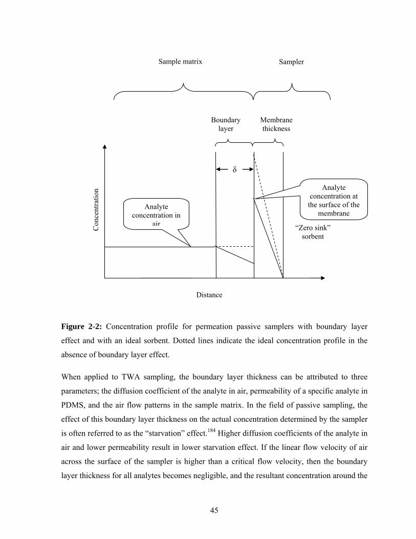
45

Figure 2-2: Concentration profile for permeation passive samplers with boundary layer

effect and with an ideal sorbent. Dotted lines indicate the ideal concentration profile in the

absence of boundary layer effect.

When applied to TWA sampling, the boundary layer thickness can be attributed to three

parameters; the diffusion coefficient of the analyte in air, permeability of a specific analyte in

PDMS, and the air flow patterns in the sample matrix. In the field of passive sampling, the

effect of this boundary layer thickness on the actual concentration determined by the sampler

is often referred to as the “starvation” effect.184 Higher diffusion coefficients of the analyte in

air and lower permeability result in lower starvation effect. If the linear flow velocity of air

across the surface of the sampler is higher than a critical flow velocity, then the boundary

layer thickness for all analytes becomes negligible, and the resultant concentration around the


air

Analyte concentration at

the surface of the membrane


Sample matrix

Membrane thickness

Distance

Con

cent

ratio

n

Boundary layer

Sampler

δ

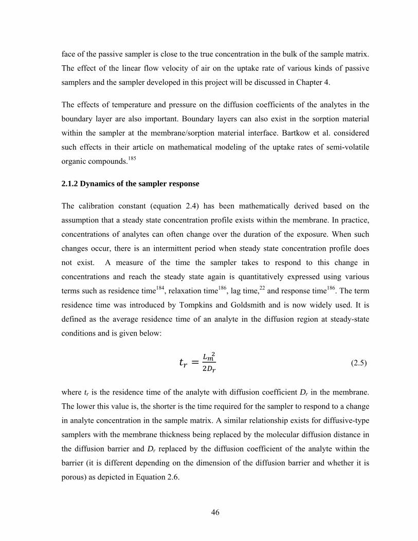
46

face of the passive sampler is close to the true concentration in the bulk of the sample matrix.

The effect of the linear flow velocity of air on the uptake rate of various kinds of passive

samplers and the sampler developed in this project will be discussed in Chapter 4.

The effects of temperature and pressure on the diffusion coefficients of the analytes in the

boundary layer are also important. Boundary layers can also exist in the sorption material

within the sampler at the membrane/sorption material interface. Bartkow et al. considered

such effects in their article on mathematical modeling of the uptake rates of semi-volatile

organic compounds.185

2.1.2 Dynamics of the sampler response

The calibration constant (equation 2.4) has been mathematically derived based on the

assumption that a steady state concentration profile exists within the membrane. In practice,

concentrations of analytes can often change over the duration of the exposure. When such

changes occur, there is an intermittent period when steady state concentration profile does

not exist. A measure of the time the sampler takes to respond to this change in

concentrations and reach the steady state again is quantitatively expressed using various

terms such as residence time184, relaxation time186, lag time,22 and response time186. The term

residence time was introduced by Tompkins and Goldsmith and is now widely used. It is

defined as the average residence time of an analyte in the diffusion region at steady-state

conditions and is given below:

(2.5)

where tr is the residence time of the analyte with diffusion coefficient Dr in the membrane.

The lower this value is, the shorter is the time required for the sampler to respond to a change

in analyte concentration in the sample matrix. A similar relationship exists for diffusive-type

samplers with the membrane thickness being replaced by the molecular diffusion distance in

the diffusion barrier and Dr replaced by the diffusion coefficient of the analyte within the

barrier (it is different depending on the dimension of the diffusion barrier and whether it is

porous) as depicted in Equation 2.6.

47

(2.6)

The diffusion coefficient of any analyte in PDMS is often four to five orders of magnitude

lower compared to that in air. However, the membrane thickness used in this project was on

the order of micrometers, whereas the diffusion distances for diffusive-type samplers are on

the order of millimeters or centimeters. Consequently, the effective residence times for both

types of passive samplers are essentially of the same order of magnitude. For example, the

residence time of toluene for diffusive-type passive samplers, GABIE and Perkin Elmer, are

4.05 s and 25.5 s, respectively.187 Considering a diffusion coefficient of 1.15 x 10-6 cm2s-1 for

the diffusion of toluene through PDMS188 and a 75 µm PDMS film thickness generally used

in this project, the residence time can be calculated to be 24.5 s. PDMS membranes are

available commercially with a thickness as low as 25 µm, which could lead to residence

times of merely 2.7 s as shown in Figure 2-3 below.

Figure 2-3: Effect of the membrane thickness on the residence time of the analytes in the

membrane.

Nevertheless, various researchers working on this aspect have determined that when the total

sampling time is substantially longer than the residence time, say 20 times, the contribution

of the error due to delayed response by the sampler is negligible.189 The TWA-PDMS

sampler is typically deployed for days or weeks, so this is more than ample time to fulfill the

above condition.

05

101520253035404550

0 20 40 60 80 100 120

Res

iden

ce ti

me

in se

cond

s

Membrane thickness in micrometers

48

2.2 Estimation of the calibration constant

The requirement that the calibration constant be known prior to sampler deployment

necessitates the analyte identity to be known prior to the sampler deployment, which is not

always possible. In such cases, it becomes important to arrive at an estimate of the calibration

constant for an analyte after analyzing the sorbent in the laboratory. For diffusive-type

samplers, such estimation boils down to using either available or estimated diffusion

coefficients of the analytes in air to calculate the calibration constants, while for permeation

passive samplers it has thus far not been possible to arrive at an estimate without conducting

tests under controlled conditions.

Various physicochemical properties of the analytes were researched to explore the possibility

of using them to develop a model for the estimation of the calibration constants. One such

property was linear temperature-programmed retention index of the analytes determined

using PDMS as the stationary phase in a capillary GC column. Such correlations were

reported in the author’s M.Sc thesis190 and by Zabiegała et al.100 The hypothesis that

calibration constants could be estimated based on the linear temperature-programmed

retention indices (LTPRI) of the analytes was developed based on the theory of permeability

of PDMS towards organic vapors and the concept of linear temperature-programmed

retention index. To understand how and why LTPRI and the calibration constant should be

related to each other, a simple mathematical approach can be developed based on the fact that

relative permeabilities of PDMS towards various analytes (and hence the calibration

constants) are a strong function of the partition coefficient, and so is LTPRI. The relationship

between these parameters is discussed in the next three sections.

2.2.1 Contribution of analyte partition coefficient to permeability

Graham described the basics of the solution-diffusion model for permeation of organic

compounds as early as in the 1800s.191 According to this model, the transfer of gas or vapor

across a polymer takes place in three steps: dissolution of the vapor molecule in the polymer,

diffusion of the molecule under a concentration gradient, and the release of the vapor from

the polymer at the opposite side of the membrane.192 It can be shown that the permeability

49

coefficient P of a molecule is a product of its diffusion coefficient D in the polymer

membrane and its partition coefficient K.

DKP= (2.6)

It has long been known that vapor molecules permeate faster through rubbery polymers (such

as PDMS) than through glassy polymers (such as Teflon®).192 The structure of PDMS is

shown in Figure 2-4. PDMS, of all the rubbery polymers, has one of the lowest diffusivity

selectivity for permeation because of the flexible (-Si-O-Si-) backbone of the polymer chains,

as well as the relatively weak binding forces between the individual segments.193 In fact,

PDMS has one of the lowest glass-transition temperatures for polymers of -127˚C which

allows long-range segmental motions even at very low temperatures. As a result, the relative

differences in permeability of vapor molecules are mostly governed by their solubility (or, in

other words, the partition coefficient) in the polymer rather than the diffusivity in the

polymer.192 Results of various studies reported in the literature support the assumption that

diffusivity of molecules in PDMS is of the same order of magnitude for most volatile organic

compounds. This is illustrated in Table 2-1, using data on diffusion and partition coefficients

reported by Kong et al. at 321 K.194 Within the homologous series, the diffusion coefficients

of the compounds decrease with increasing molecular size, but the relative decrease is

marginal when compared to the exponential increase in the partition coefficients of the

compounds.

Figure 2-4: The structure of PDMS (reproduced from ref. 195)

50

Table 2-1: Partition coefficients and diffusion coefficients of n-alkanes (based on ref. 194).

Compound Diffusion coefficient D x1010 (m2 sec-1)

Partition coefficient K

n-pentane 6.5 40 n-hexane 6.0 95 n-heptane 5.3 218 n-octane 4.2 516 n-nonane 2.9 1267

A mathematical relationship between the calibration constant and the partition coefficient can

then be derived under the assumption that D is constant for volatile organic compounds.

Under these conditions, taking the natural logarithms of both sides of Equation (2.3), one

gets,

KZk lnln −= (2.7)

where Z is a constant defined by:

⎥⎦⎤

⎢⎣⎡=

ADL

Z mln (2.8)

In a homologous series of compounds, even though the diffusion coefficients are of the same

order of magnitude, they typically decrease with increasing molecular weight of the

compound. Under such conditions, constancy of the D×MW product can also be considered,

and the correlations explored.

The assumption that the product of diffusion coefficient and molecular weight can be

considered a constant was studied for the diffusion coefficients available from literature

sources, and the results are tabulated in Tables 2-2194 and 2-3.196 For the n-alkane

homologous series (Table 2-2), the relative standard deviations (RSD) of D, ln D, and ln

(MW*D) show that the spread in ln (MW*D) was negligible when compared to the 29% RSD

for D and 2.6% RSD for ln D. Similarly, for the n-alcohols homologous series (Table 2-3),

the RSD of D, ln D, and ln (MW*D) show that the spread in ln (MW*D) was negligible when

51

compared to the 43% RSD for D and 2.5% RSD for ln D. These values are as expected for a

homologous series of compounds.

Table 2-2: Variation in diffusivity with molecular weight for n-alkanes (based on ref.194)

Compound Diffusion

coefficient D x1010 (m2 sec-1)

Molecular weight (MW)

MWxDx1010 ln D ln (MWxD)

n-pentane 6.5 72.15 470 -21 -17

n-hexane 6.0 86.177 520 -21 -17

n-heptane 5.3 100.203 530 -21 -17

n-octane 4.2 114.23 480 -22 -17

n-nonane 2.9 128.257 370 -22 -17

Average 5.0 100.2 474 -21 -17

Standard deviation 1.4 22.18 62 0.55 0

% RSD 29 22.13 13 2.6 0

Table 2-3: Variation in diffusivity with molecular weight for n-alcohols (based on ref. 196).

Compound Diffusion

coefficient D x1010 (m2 sec-1)

Molecular weight (MW)

MWxDx1010 ln D ln (MWxD)

Methanol 10 32.042 320 -21 -17

Ethanol 7.1 46.069 330 -21 -17

Propanol 6.2 60.096 370 -21 -17

Butanol 5.5 74.122 410 -21 -17

Pentanol 5.1 88.149 450 -21 -17

Hexanol 4.2 102.176 430 -22 -17

Heptanol 4.1 116.203 480 -22 -17

Octanol 3.9 130.23 510 -22 -17

Nonanol 3 144.256 430 -22 -17

Decanol 2.5 158.283 400 -22 -17

Average 5.2 95.16 413 -21.5 -17

Standard deviation 2.21 42.47 61 0.53 0

% RSD 43 44.63 15 2.5 0

52

With the assumption that the product of diffusion coefficient and molecular weight can be

considered a constant , the mathematical relationship takes the form

KQMW

k lnln −=⎥⎦⎤

⎢⎣⎡

(2.9)

where Q is a constant defined as

⎥⎦⎤

⎢⎣⎡

×=

MWADL

Q mln (2.10)

Equations 2.7 and 2.9 show the relationship between the calibration constant and partition

coefficient. The calibration constant can then be related to LTPRI based on the relationship

between LTPRI and the partition coefficient as described in the next section.

2.2.2 Relationship between the linear temperature-programmed retention index and

partition coefficient of the analyte

Partition gas chromatography involves the partitioning of the solute between a liquid

stationary phase and a gaseous mobile phase. Therefore, the retention properties of a

compound in such a chromatographic separation are a function of the analyte partition

coefficient between the carrier gas and the stationary phase (PDMS in this case). Under

isothermal conditions, the partition coefficient of a solute at a given temperature is related to

the retention time of the solute in the following manner,197

m

s

m

mr

m

r

VVK

ttt

tt

=−

='

(2.11)

where t`r is the adjusted retention time, tm is the retention time of an un-retained compound, tr

is the retention time of the solute, K is the partition coefficient of the solute, Vs is the volume

of the stationary phase, and Vm is the volume of the mobile phase.

53

Van den Dool and Kratz198 introduced the concept of LTPRI (dimensionless), which involves

calculation of the retention index while achieving chromatographic separation under the

conditions of linear temperature programming. LTPRI is defined as:

n

tttt

LTPRInn

nr 1001001

+⎥⎦

⎤⎢⎣

⎡−−

=+

(2.12)

where tr is the retention time of the analyte, tn is the retention time of the n-alkane eluting

directly before the analyte, tn+1 is the retention time of the n-alkane eluting directly after the

analyte, and n is the number of carbon atoms in the n-alkane eluting directly before the

analyte. The exact correlation between LTPRI and the partition coefficient is complicated,

and involves fluid dynamics inside the capillary column.199 However, various researchers

working on determining empirical relationships and/or mathematical approximations have

found that LTPRI for a homologous series of compounds is related to the partition coefficient

of the analytes at a particular temperature as9

BKNLTPRI += ln (2.13)

where N and B are constants. The relationship for a homologous series of n-alkanes can be

quickly verified using data obtained by Kloskowski et al.200 at 298 K using a capillary

column with PDMS stationary phase (Figure 2-5). The correlation was found to be excellent

with a correlation coefficient of 0.9999. Further validity of this concept can be drawn from

data presented by Martos et al., who used solid phase micro-extraction techniques for

compounds including benzene, toluene, ethyl benzene, n-propyl benzene, n-pentyl benzene

and n-hexyl benzene among others (Figure 2-6).201 The above relationship was successfully

used to estimate the calibration constants of various analytes in solid-phase microextraction

with PDMS-coated fibres.

54

Figure 2-5: Partition coefficient – LTPRI correlation for n-alkanes (based on ref. 200).

Figure 2-6: Partition coefficient – LTPRI correlation for aromatic compounds (based on ref. 201).

Since relative calibration constants are mainly a function of the partition coefficients of the

analytes between air and PDMS as discussed in section 2.2.1, the relationship between

LTPRI and the partition coefficient discussed in this section can be used to correlate

calibration constants with LTPRI.

ln(K ) = 0.0094 * LTPRI - 0.2557 R2 = 0.9994

0.00

2.00

4.00

6.00

8.00

10.00

12.00

400 600 800 1000 1200 1400 Linear Temperature-Programmed Retention Index

ln (K

)

ln(K ) = 0.01 * LTPRI - 0.8777 R2 = 0.9999

0.00

2.00

4.00

6.00

8.00

10.00

12.00

400 600 800 1000 1200 Linear Temperature-Programmed Retention Index

ln ( K )

55

2.2.3 The calibration constant – LTPRI correlation

From equations (2.7), (2.8) and (2.9), the relationship between the calibration constant k and

LTPRI can theoretically be obtained and can be studied under two scenarios:

Case 1: When D is assumed to be constant, equations (2.7) and (2.13) suggest that ln(k) is

directly proportional to LTPRI. If this is true, then the major advantage would be the ability

to estimate the calibration constants for analytes without knowing their identity (because it is

not required to know the identity of a compound to determine its LTPRI)

Case 2: When ln (D×MW) is considered constant, equations (2.9) and (2.13) suggest that

ln(k/MW) is directly proportional to LTPRI. In this case, the calibration constant could be

estimated using LTPRI, but the identity of the compound would have to be known in order to

determine its molecular weight. The identities of unknown analytes (thus their molecular

weights) can often be established when using mass spectrometry for analyte detection.

It should be noted that the physical form of PDMS within the capillary column may differ

from that which forms the membrane. The physical nature of PDMS depends on the degree

of polymerization, cross-linking and the amount of fillers added in the manufacturing

process. A low degree of polymerization (short chain lengths) and cross-linking result in a

liquid-like physical form. A high degree of polymerization and cross-linking, along with

addition of fillers such as SiO2, result in the formation of a more rigid material. Cramers et al.

noted that the LTPRI was nearly the same on PDMS stationary phases with and without

cross-linking.202 Therefore, the hypothesis that the calibration constant should be related to

LTPRI should still be valid.

Calibration constants of 41 model compounds having different functional groups were

determined and the above two cases were investigated. The details of the experiments will be

discussed in the next Chapter.

56

CHAPTER 3

Experimental determination of the calibration constants and their

correlation with physicochemical properties of the analytes

The knowledge of the calibration constants of the sampler towards the target analytes is

required to determine the analytes’ concentration in the vapor phase. When the calibration

constant has not been experimentally determined, it is desirable to be able to estimate it based

on the physicochemical properties of the analytes and the membrane material used for the

fabrication of the sampler. The present chapter deals with the experimental determination of

the calibration constants and using them to arrive at a model for the estimation of the

calibration constants of analytes for which they are unknown.

The passive sampler design developed in this project and the idea of using physicochemical

properties of the analytes for estimating the calibration constants is based on a similar design

and concept first presented by Zabiegała, Górecki and Namieśnik.100 The reason for

redesigning the sampler and proposing a different theoretical model for the estimation of the

calibration constant of the newly designed sampler was first presented in the author’s M.Sc

thesis.190 Since the project presented in this thesis was a logical continuation of that presented

in the author’s M.Sc. thesis, a brief background of that research and its outcomes will first be

provided.

3.1 Background to original sampler design, development of the new design and previous

research observations

The original design of the sampler, as shown in Figure 3-1, was first developed at the Gdańsk

University of Technology (Poland) using a PDMS membrane as the permeation barrier and

activated carbon as the sorbent.100 The sampler was equipped with a metal screen (2) for

mechanical protection of the membrane, and the membrane (4) was mounted between this

screen and the PTFE washer (7). Active carbon was used as the sorbent (5). It was held in

contact with the membrane by a glass wool plug (6) and plastic plug (11) screwed into the

body of the sampler (8). The above ensemble was mounted in a screw cap (1), which was

57

prevented from loosening by tightening a setscrew (12). The body of the sampler (8) and the

internal chamber of the sampler were sealed using an O-ring (9) made of Buna-S rubber.

Figure 3-1: Passive sampler designed at the Gdańsk University of Technology. 1. screw cap;

2. protective screen mount; 3. protective screen; 4. PDMS membrane; 5. active carbon; 6.

glass wool; 7. washer; 8. main body; 9. O-ring; 10. opening for a screw-in holder; 11. plug;

12. set screw (reproduced from ref. (100).

This permeation-type passive sampler was equipped with a 50 µm thick PDMS membrane

and Zabiegała et al. determined the calibration constants of this sampler towards various

groups of analytes. During the author’s M.Sc. thesis work, the same sampler design but

without the set screw shown in Figure 3-1 was used in the experiments. As a 50 µm thick

membrane was not available at that time, a 75 µm thick membrane was employed instead.

Also, the same experimental setup (as used by Zabiegała et al.) was used with some

improvements in the flow controlling system in the experimental setup. The calibration

constants obtained by the author for n-alkanes did not match the data published by Zabiegała

et al., according to which there was a linear relationship between LTPRI and k (as against a

linear relationship between ln(k) vs. LTPRI discussed in the Chapter 2), as shown in Figure

58

3-2. This resulted in a detailed investigation to explain the discrepancy and was one of the

main focuses of the author’s M.Sc. thesis.

Figure 3-2: Calibration constant vs. LTPRI correlation for n-alkanes obtained by Zabiegała

et al. (reproduced from ref (100)).

The investigations revealed the important reasons for the observations. The thickness of the

membrane used earlier (50 µm) was different from that used by the author (75 µm). This

would affect the uptake rates of the sampler towards various analytes to a different extent, as

the starvation effect is different for different analytes (discussed in more detail in Chapters 1,

4, 6 and 7). This was further exaggerated as there was no proper air circulation inside the

exposure chamber in which the samplers were exposed to standard test gas atmosphere to

determine the calibration constants. A new exposure chamber was then built (described in

detail later in this chapter), in which a fan was incorporated to allow proper air circulation

around the sampling surface of the samplers. The calibration constants obtained using the

new chamber and for the same analytes by the author along with the calibration constants

obtained by Zabiegała et al. are shown in Table 3-1.

y = -0.0003x + 0.3829R² = 0.993

0.00

0.05

0.10

0.15

0.20

0.25

200 400 600 800 1000 1200

(cal

ibra

tion

cons

tant

)

LTPRI

k vs. LTPRI for n-alkanes

59

Table 3-1: Calibration constants and retention indices for n-alkanes observed by Zabiegała et

al. and Seethapathy (reproduced from ref. (100) and (190))

Compounds LTPRI

Calibration constant reported by

Zabiegała et al., k (min cm-3)

Calibration constant reported by the author of this thesis

with modified experimental set up, k (min cm-3)

n-pentane 500 0.230 n/a

n-hexane 600 0.184 0.156

n-heptane 700 0.160 0.087

n-octane 800 0.132 0.054

n-nonane 900 0.100 0.037

n-decane 1000 0.064 0.023

The calibration constants obtained by the author were lower than those reported by Zabiegała

et al., which confirmed that starvation effect was indeed reduced to a great extent by the fan

in the exposure chamber. Further, a plot of ln(k) vs. LTPRI (Figure 3-3) using the data

obtained by the author supported the hypothesis presented in this thesis (and earlier in the

Master’s thesis). This could further be confirmed based on the data by Kong et al., which

indicate that the permeability of PDMS (which is inversely proportional to the calibration

constant) towards n-alkanes from pentane to nonane increases exponentially as shown in

Figure 3-4.194 It was difficult to recognize this correlation from the data reported by

Zabiegała et al., as the calibration constants were all within one order of magnitude. Should

the differences be greater than that, the true character of the relationship could have been

possibly observed.

60

Figure 3-3: ln (k) vs. LTPRI correlation for n-alkanes observed with a fan incorporated in

the calibration chamber (from ref. (190)).

Figure 3-4: Data showing exponential increase in the permeability of PDMS towards n-

alkanes with an increase in LTPRI (based on ref. (194)).

Though the sampler design shown earlier worked well, a new design was proposed during

the author’s M.Sc. thesis work for three main reasons:

(i) To reduce the cost of sampler fabrication to enable large scale studies which

require large numbers of samplers,

ln(k) = -0.0047 * LTPRI + 0.8695R2 = 0.9947

-4.00-3.50-3.00-2.50-2.00-1.50-1.00-0.500.00

400 500 600 700 800 900 1000 1100

ln(k

)

LTPRI

ln(k) vs. LTPRI correlation for n-alkanes

R² = 0.9943

0500

10001500200025003000350040004500

400 500 600 700 800 900 1000

Perm

eabi

lity

(Px1

010m

2 sec

-1)

LTPRI

PDMS permeability vs. LTPRI for n-alkanes

61

(ii) To reduce the area of the cross section of the membrane exposed to the sample

matrix, and consequently reduce the starvation effect, and

(iii) To allow for sampling and sample extraction in the same sampler housing if

required.

The new design functioned in exactly the same manner as the earlier design, but was based

on a 1.8 mL crimp-cap auto sampler vial used as a housing for the PDMS membrane and the

sorbent (described later in detail). Various experiments were conducted to determine the

calibration constants of this sampler towards n-alkanes (hexane to decane), aromatic

hydrocarbons (benzene, toluene, ethyl benzene, propyl benzene, and butyl benzene) and

chlorinated compounds (1,1-dichloroethylene, dichloromethane, cis-dichloroethene,

chloroform, 1,1,1-trichloroethane, 1,2-dichloroethane, trichloroethylene and

tetrachloroethylene). The results had confirmed a linear correlation between ln(k) and LTPRI

for n-alkanes and aromatic hydrocarbons, but not the chlorinated compounds for which there

was a linear correlation between ln (k/MW) and LTPRI. Based on these observations and to

further investigate the LTPRI and calibration constant relation, more model compounds from

moderately polar esters to polar alcohols were chosen for further experimentation, which

forms a part of this thesis.

The experimental setup described in this chapter, as well as the methods of determining the

calibration constants were the same as those used during the author’s M.Sc. thesis work. The

calibration constants of the sampler towards n-alkanes and aromatic hydrocarbons were

determined again to confirm the correlation and are presented in this thesis. The calibration

constants of the newly designed sampler towards chlorinated compounds determined during

the author’s previous work were essential in order to arrive at the overall relationship

between LTPRI and the calibration constants and were extensively used for field sampling

applications discussed in Chapters 6 and 7. Therefore, the data related to the chlorinated

compounds as well as the model developed for estimating the calibration constants, are

included in this thesis as well. However, only those data and methods necessary and

sufficient to enable the readers to understand the overall functioning of the sampler have

been included in this thesis.

62

3.2 Chemicals used in the experiments

High purity CS2 required for the preparation of standard solutions of the analytes for gas

chromatographic quantification and for analyte desorption from sorption tubes and passive

samplers was purchased from VWR CANLAB (Mississauga, ON). Chromatography grade

compressed air, helium, nitrogen, and hydrogen were purchased from Praxair (Kitchener,

ON). All high purity, analytical grade chemicals were purchased from Sigma-Aldrich

(Bellefonte, PA). The minimum purity, molecular weights, boiling points and CAS numbers

of these chemicals are listed in Table 3-2.

Table 3-2: Purity and physical properties of model compounds used in the experiments.

Group Name of the compound CAS-No % Purity Molecular weight

Boiling point (˚C at STP)

Esters

Ethyl acetate 141-78-6 99.7 88.106 77.1

Propyl acetate 109-60-4 99.5 102.133 102

Methyl butyrate 623-42-7 99 102.133 102-103

Sec-butyl acetate 105-46-4 99 116.160 112

Ethyl butyrate 105-54-4 99 116.160 121

Butyl acetate 123-86-4 99.7 116.160 126.1

Propyl butyrate 105-66-8 99 130.187 142-143

Butyl butyrate 109-21-7 98 144.213 166

Chlorinated compounds

1,1- Dichloroethylene 75-35-4 98 96.944 31.7

Dichloromethane 75-09-2 99 84.933 39.8

Cis-1, 2-Dichloroethylene 156-59-2 99 96.944 60

Chloroform 67-66-3 99 119.378 61.7

1,1,1-Trichloroethane 71-55-6 98 133.405 74.1

1,2-Dichloroethane 107-06-2 98 98.960 83.5

Carbon tetrachloride 56-23-5 99 153.823 76.7

Trichloroethylene 79-01-6 99 131.389 86.7

63

Table 3-2 (continued): Purity and physical properties of model compounds used in the

experiments.

Group Name of the compound CAS-No % Purity

Molecular weight

Boiling point (˚C at STP)

n-Alkanes

n-hexane 110-54-3 99.5 86.177 69

n-heptane 142-82-5 99 100.203 98.4

n-octane 111-65-9 99 114.230 126

n-nonane 111-84-2 99 128.257 150.8

n-decane 124-18-5 99 142.284 174.1

Aromatic hydrocarbons

Benzene 71-43-2 99 78.113 80.1

Toluene 108-88-3 99 92.140 110.6

Ethyl benzene 100-41-4 99 106.167 136.2

Propyl benzene 103-65-1 98 120.194 159

Butyl benzene 68411-44-9 99 134.221 183

Alcohols

2-methyl-1-propanol 78-83-1 99 74.122 107.9

n-butanol 71-36-3 99 74.122 117.6

2,3-dimethyl-2-butanol 594-60-5 99 102.176 119

n-pentanol 71-41-0 99 88.149 137.9 - 139

2-hexanol 626-93-7 99 102.176 136

2,4-dimethyl-3-pentanol 600-36-2 99 116.203 139

n-hexanol 111-27-3 99 102.176 156 - 157

n-heptanol 111-70-6 98 116.203 176

2-octanol 123-96-6 99 130.230 180

2-ethyl-1-hexanol 104-76-7 99 130.230 183

n-octanol 111-87-5 99 130.230 195

2-methyl-1-butanol 137-32-6 99 88.149 129

3-Octanol 589-98-0 98 130.230 174-176

6-methyl-2-heptanol 4730-22-7 99 130.230 172

64

3.3 Experimental

In this section, the design of the permeation passive samplers will first be presented. The

general aspects of the experimental setup will then be described, followed by detailed

experimental methods employed for the determination of LTPRI and the calibration

constants of the sampler towards various analytes.

3.3.1 Passive sampler design

A simple passive sampler was designed and fabricated using a 1.8 mL standard mouth, crimp

cap, chromatography auto-sampler vial, a PDMS membrane and a sorbent, as illustrated in

Figure 3-5. The PDMS membrane (Product code: SSP-M823) used in the samplers was

procured from Specialty Silicone Products Inc., (Ballston Spa, NY). The membrane had a

nominal thickness of 75 µm. Even though the information was provided that silicon dioxide

was added as a filler to increase the physical strength of the membrane, the manufacturer did

not reveal its exact percentage in the finished product. The translucent PDMS membrane was

supplied with a brown, nylon support sheet. The membrane along with the nylon support

sheet was first cut to the shape of the top surface of the 1.8 mL glass vial using a cutting tool

shown in Figure 3-6. The membrane was then separated from the support and weighed. Since

the specific gravity of the commercially available PDMS membrane (1.17 ± 0.2)203 and the

area cut by the cutting tool were constant, the weight of the membrane served as a control for

the membrane thickness. The thicknesses of the membranes procured were measured at the

Department of Mechanical Engineering, University of Waterloo, using an Olympus U-

PMTVC optical microscope (Tokyo, Japan) coupled to a digital image capture system. A

typical cross section of the membrane as observed using the optical microscope is depicted in

Figure 3-7.

65

Figure 3-5: 1.8 mL crimp cap vial-based permeation passive sampler.

The samplers were then fabricated using the procedure illustrated in Figure 3-8. Anasorb

747®, an activated carbon-based sorbent available commercially in bulk quantities of 100 g

from SKC Inc., (Philadelphia, PA), was used as the sorbent for the samplers. Approximately

250 mg of Anasorb 747® were weighed into the glass vial and the PDMS membrane was

placed on top of the vial. An aluminum cap was then placed on top of the membrane and

crimped using a crimper. A support made of heavy gauge PTFE tape procured from

G.F.Thompson Co. Ltd. (Newmarket, ON), also shown in Figure 3-9, was attached to the

Figure 3-6: Photograph of a membrane

with nylon backing and the membrane

cutting tool

Figure 3-7: Photograph of a membrane cross-

section

Aluminum crimp cap

1.8 mL crimp top vial

PDMS membrane

Sorbent

Membrane thickness

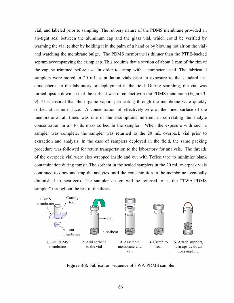
66

vial, and labeled prior to sampling. The rubbery nature of the PDMS membrane provided an

air-tight seal between the aluminum cap and the glass vial, which could be verified by

warming the vial (either by holding it in the palm of a hand or by blowing hot air on the vial)

and watching the membrane bulge. The PDMS membrane is thinner than the PTFE-backed

septum accompanying the crimp cap. This requires that a section of about 1 mm of the rim of

the cap be trimmed before use, in order to crimp with a competent seal. The fabricated

samplers were stored in 20 mL scintillation vials prior to exposure to the standard test

atmospheres in the laboratory or deployment in the field. During sampling, the vial was

turned upside down so that the sorbent was in contact with the PDMS membrane (Figure 3-

9). This ensured that the organic vapors permeating through the membrane were quickly

sorbed at its inner face. A concentration of effectively zero at the inner surface of the

membrane at all times was one of the assumptions inherent in correlating the analyte

concentration in air to its mass sorbed in the sampler. When the exposure with such a

sampler was complete, the sampler was returned to the 20 mL overpack vial prior to

extraction and analysis. In the case of samplers deployed in the field, the same packing

procedure was followed for return transportation to the laboratory for analysis. The threads

of the overpack vial were also wrapped inside and out with Teflon tape to minimize blank

contamination during transit. The sorbent in the sealed samplers in the 20 mL overpack vials

continued to draw and trap the analytes until the concentration in the membrane eventually

diminished to near-zero. The sampler design will be referred to as the “TWA-PDMS

sampler” throughout the rest of the thesis.

2. Add sorbent to the vial

sorbent

vial

3. Assemble membrane and

cap

4. Crimp to seal

5. Attach support, turn upside down

for sampling

1. Cut PDMS membrane

cut membrane

Cutting tool

PDMS membrane

Figure 3-8: Fabrication sequence of TWA-PDMS sampler

67

Figure 3-9: Deployment of the TWA-PDMS sampler in the field

A summary of the reasons for the use of the specific design and material of fabrication has

been provided below for the benefit of the readers at this point of the thesis. Detailed

explanations of the advantages of this design will be dealt with in the remainder of the thesis.

• The 1.8 mL crimp top vial used in the fabrication of the sampler is the same as the vial used

for autoinjectors in most gas chromatography instruments. The same vial can also be used

for solvent desorption. This drastically reduces the sample preparation steps, reduces cost

and errors, and allows for potential complete automation of the sample preparation and

quantification process.

• Polydimethylsiloxane used for the membrane has properties that are well suited for passive

sampling of VOCs from air. It has high permeability towards many organic compounds,

low permeability for water, and low energy of activation of permeation; it is easily available

in membrane form, inexpensive and has been studied and used widely since the 1960’s. It is

the same material as that used as the stationary phase in capillary GC columns, which (as

discussed in Chapter 2) provides a valuable opportunity for estimating uptake rates using a

correlation to published GC retention indices.

• Anasorb 747® is a granular, activated carbon-based sorbent which has been widely used for

sorption of volatile organic compounds in various other active and passive sampling

systems. This commercially available sorbent is often touted as a universal sorbent for the

sorption of volatile organic compounds and analyte recoveries from the sorbent after

solvent desorption are generally high and reproducible.

68

3.3.2 Experimental setup

The function of the experimental setup was to generate a test gas atmosphere with

measurable concentrations of the analytes, where the passive sampler could be exposed for a

predetermined amount of time for determining its calibration constant towards the analytes.

The overall design of the experimental setup is illustrated in Figure 3-10. Nitrogen was

passed through an air purifier (containing activated carbon) to remove traces of VOC

impurities at a flow rate controlled by a mass flow controller (model MDF-52000L0N-0L)

purchased from Pneucleus Technologies Inc., (Hollis, NH). The mass flow controller had an

operating range of 0 to 1000 mL/min and was connected in series with an MKS Instruments

(Andover, MA) Type 247 4-channel readout system for setting and monitoring the flow. The

purified gas was then passed through a standard gas mixture generator whose design is

described next.

Figure 3-10: Schematic of the experimental setup used for the determination of the

calibration constants.

The standard gas mixture generator used permeation tubes as the source for analyte vapors.

Neat liquid enclosed in these permeation tubes (shown in Figure 3-11) permeated through the

walls of the tube at a constant rate, and the vapors were swept by purified gas which entered

the calibration chamber. The permeation tubes were made from virgin PTFE tubing cut into

Air purifier

Flow controller

Standard gas mixture generator

Thermostated

exposure

chamber

Sorbent sampling tube

High pressure N2 source

Soap bubble flow meter

Suction pump with needle valve for

flow control

Vent to fumehood

Stirrer

69

segments of the desired lengths. The tubes prepared in this way were filled with neat liquids

of the test compounds and sealed by means of PTFE plugs and Swagelok® ferrules

compressed using a custom-made, removable fitting.204 The PTFE tubes used for the

fabrication of the permeation tubes had an outer diameter of ¼” and a wall thickness of 250

μm. The PTFE plugs were standard, ¼” diameter rods, which were machined on a lathe to

reduce the thickness by approximately 250 μm to tightly fit the tubing. The brass Swagelok®

ferrules were those used for standard ¼” outer diameter metal tubing. The permeation tube

lengths ranged from 5 cm to 10 cm, depending on the volatility of a compound (longer tubes

for less volatile compounds so as to have larger surface area of permeation, and hence

increased flux). Depending on the composition of the standard gas mixture required, the

respective permeation tubes (each tube containing one neat liquid) were enclosed in a flow-

through vessel maintained at a constant temperature by placing them inside a GC oven as

shown in Figure 3-12. Different sets of compounds were thermostated at different

temperatures based on the permeation rates of the compounds through PTFE. The outlet of

the standard gas mixture generator was connected to the inlet of the calibration chamber. The

calibration chamber design and construction are detailed in the next paragraph.

70

Brass ferrule

PTFE Plug Neat liquid

PTFE tube

Figure 3-11: (A) Photograph and (B) schematic of a permeation tube used for the generation

of standard test gas atmospheres.

Figure 3-12: Photograph of the standard gas mixture generating system.

GC oven

Mass flow controller

Permeation tubes

A

B

71

A schematic and a photograph of the calibration chamber used for the experiments are shown

in Figures 3-13 and 3-14, respectively. The calibration chamber was constructed using a 10-

liter cylindrical glass jar. A PTFE plate of ¼” thickness was used as the top lid for the glass

jar, with an O-ring (made of PTFE-encapsulated Viton) between the plate and the jar for

better sealing. The PTFE plate was held in place with the help of two aluminum plates, one

placed on top of the Teflon® plate and another below the glass jar and the cooling jacket.

These plates were held together by means of stainless steel rods, threaded on both ends,

which were fixed to the bottom and top aluminum plates with the help of nuts. A motor

(model Number JB2PO21N, Universal Electric Company, MI) was fixed on top of the

aluminum plate, and a hole was drilled in the centre of the PTFE and aluminum plates to

allow the shaft from the motor to run through this hole. A fan blade made of high-density

polyethylene was attached to the bottom of the shaft. The motor itself was connected to a

Powerstat® variable autotransformer (model 3PN116B, Superior Electric Company, CT) to

enable control of the speed of the circulation fan. Also connected to the chamber was a ¼”

diameter copper tubing inlet, through which the standard gas mixture entered the chamber.

Holes were drilled in the segment of the inlet tubing positioned parallel to the bottom of the

chamber to allow uniform introduction of the analyte gas mixture. Eight holes were drilled

through the top plates (aluminum and PTFE) with diameters small enough to hold the vial-

based passive samplers snugly, and the vials were inserted membrane down during exposure. The whole chamber was placed in a thermostated jacket and the outside of the jacket was

insulated by wrapping it with glass wool insulation material. The calibration chamber was

maintained at the required temperature throughout the period of sampling by circulating

radiator fluid through the jacket with the aid of a circulation thermostat (model number 000-

5744, HAAKE, Germany). The ½” inner diameter rubber tubing connecting the thermostat

and the chamber were also wrapped with the glass wool insulation material.

72

Figure 5: Calibration chamber

Inlet

Hole to insert sampler

PTFE plate

Gas mixture delivery tube

Jacket

Aluminum plate

Fan blade

Glass jar

Vent

Tubing for active sampling

Variable speed motor

Perforated portion of tube

SS support

Figure 3-13: Schematic of the calibration chamber used for the exposure of the TWA-PDMS

samplers to standard test gas mixtures.

73

Figure 3-14: Photograph of the top part of the calibration chamber showing the sampler

ports, test gas mixture inlet, motor and the test gas mixture outlet ports.

The passive samplers, inserted into the sampler ports of the calibration chamber, were thus

exposed to a dynamic standard gas mixture. A piece of 1/8” stainless steel tubing inserted

into the chamber through the vent was used to draw a sample of the chamber atmosphere

through a sorption tube. The custom-made sorption tubes (fabricated by the glass blowing

shop, University of Waterloo) were loaded with 300 mg of Anasorb 747® in the sample

section and 100 mg in the back-up section, as shown in Figure 3-15.

Figure 3-15: Schematic of a sorption tube used for the active sampling to determine analyte

concentrations in the calibration chamber.

Motor to rotate the fan blade

Test gas mixture inlet

Sampler ports

Test gas mixture outlet

Sorbent sampling section

Cotton plugs

Sorbent back-up section

Sample air in

Sample air out

74

The sample was drawn at a constant rate of approximately 100 mL/min using a suction pump

(Model MB-21) procured from Metal Bellows Corp. (Shanon, MA). The sample flow rate

was measured using a bubble flow meter. Analyte concentrations in the calibration chamber

were then determined based on the analyte mass trapped by the sorbent tube (determined by

gas chromatography) in a given time, and the sample flow rate. These concentrations were

then used to calculate the calibration constants of the samplers towards the analytes.

3.4 Experimental methods

In this section, the method used for the determination of LTPRI will first be described,

followed by the determination of the calibration constants to enable the investigation of the

correlation between the two parameters.

3.4.1 Determination of LTPRI

By definition, the retention indices of n-alkanes are 100 times the number of carbon atoms

they contain (for example, it is 500 for n-pentane). Determination of LTPRI of all other

analytes required the determination of their respective retention times, as well as the retention

times of two n-alkanes (differing in number of carbon atoms by one) such that one of the

alkanes had retention time shorter than the analyte, and the other longer than that of the

analyte (Section 2.2.2). An Agilent 6890 GC (Santa Clara, CA) equipped with a split-

splitless injector, an FID and an ECD was used for the analysis with the method described in

Table 3-3. To correlate the calibration constants to LTPRI, it was necessary to use a

capillary column with 100% PDMS stationary phase. The column was procured from Restek

(Bellefonte, PA). For the determination of the LTPRI of aromatic hydrocarbons, a mixture of

n-alkanes in CS2 (from pentane to undecane) was prepared at concentrations of

approximately 100 µg/mL each in CS2. This solution was used for the determination of the

retention times of the n-alkanes. Individual solutions of all the aromatic hydrocarbons listed

in Tables 3-1a were also prepared at approximately 100 µg/mL in CS2 and were used for the

determination of the respective analyte’s retention times for peak identification. Finally,

another solution containing approximately 100 µg/mL of all the n-alkanes and aromatic

hydrocarbons in CS2 was prepared. This solution was injected 6 times, and the averages of

75

the retention times of each compound from the 6 injections were used for the calculation of

LTPRI.

The LTPRI of different groups of compounds were determined at different points during the

course of the project. The same method as described above for aromatic hydrocarbons was

used for the determination of LTPRI of chlorinated compounds listed in Table 3-2. For the

determination of the LTPRI of alcohols and esters, the same methods was used but with a

Thermo Electron Corporation Focus GC (Waltham, MA) equipped with a split-splitless

injector and an FID. The LTPRIs determined were then used for the investigation of their

correlation with calibration constants whose determination is discussed next.

Table 3-3: Gas chromatographic method used for the determination of LTPRI.

GC Instrument Agilent Technologies model 6890 GC

Detector Flame Ionization Detector at 300˚C

Injection mode Split, 275˚C, auto-injector

Split ratio 1:10

Injection volume 1 μL

Carrier gas Helium at 1.2 mL/min Oven temperature

program 35˚C, 7˚C/min to 220˚C, held for 2 min

Data acquisition and processing Chemstation software (Agilent)

Capillary column RTX-1 (100% polydimethylsiloxane), 30 m x 0.25 mm, 0.25 μm film thickness

3.4.2 Determination of the calibration constants

The calibration constants were determined using equation 3.1:

MtCk 0= (3.1)

76

The knowledge of the extraction efficiency of the analytes from Anasorb 747® was required

to determine both the analyte mass trapped in the sampler (M) and its concentration (C0) in

the calibration chamber (by active sampling method using sorption tubes), and hence the

method used for the determination of the extraction efficiency will be described next. The

determination of the analyte mass trapped in the sampler (M) and the concentration of the

analyte (C0) in the calibration chamber will then be detailed.

3.4.2.1 Determination of analyte recovery rates from Anasorb 747®

Recoveries of all 41 compounds of interest from the Anasorb 747® sorbent were determined

prior to the exposure experiments. This involved preparation of a stock solution of the

respective analytes in CS2, followed by the addition of 10 μL aliquots of this stock solution to

six 4 mL vials containing 250 mg of Anasorb 747® each. The vials were capped and allowed

to remain at room temperature for 24 hours for equilibration. Even though the extraction

efficiency from Anasorb 747® was reported to be high for many VOCs using CS2 as the

desorption solvent (used at later stages of the project for field sampling and analysis), the

extraction efficiency could be marginally increased according to the manufacturers

specifications by using a polar solvent along with CS2 for the extraction. Consequently,

isopropyl alcohol (IPA) was used as a cosolvent in proportions depending on the polarity of

the analytes studied. For alkanes and aromatic hydrocarbons, desorption of the analytes from

the sorbent was performed by adding 1 mL of CS2 to each of the six 4 mL vials, followed by

shaking intermittently for 30 minutes. For alcohols, a 50:50 mixture of IPA and CS2 was

used for the extraction. For esters and chlorinated compounds, a 1% solution of IPA in CS2

was employed. Some of the alcohols had similar retention times under the temperature

programming conditions employed. To avoid difficulties imposed by co-elution, the

recoveries were determined by analyzing 3-octanol, 2-methyl-1-butanol and 6-methyl-2-

heptanol separately from the remaining alcohols listed in Table 3-2. The resulting extracts

were transferred to 100 μL inserts placed inside 1.8 mL crimp-top vials, and the analyte

amounts were quantified by GC. For the determination of the extraction efficiency of n-

alkanes and aromatic hydrocarbons, the Agilent 6890 GC with the method described in Table

3-3 was used. A Thermo Focus GC with Chromquest data acquisition software was used

77

instead of the Agilent GC for quantifiying alcohols and esters by gas chromatography using

the method described in Table 3-3.

In the case of chlorinated compounds, desorption was performed using a 1% solution of IPA

in CS2. Since the retention times of 1,1-dichloroethylene (1,1-DCE) and dichloromethane

(DCM) were close with 100% PDMS-based stationary phase capillary columns, a slightly

more polar HP-5 stationary phase (95% methyl and 5% phenyl) was used for their separation

and quantification. The chromatographic separation and quantification was performed using

the method detailed in Table 3-4.

Table 3-4: Gas chromatographic method used for the quantification of chlorinated

compounds.

GC Instrument Agilent Technologies, 6890 GC

Detector Electron Capture Detector at 350˚C

Injection mode Split, 275˚C

Split ratio 1:10


Carrier gas Helium at 1.2 mL/min

Oven temperature program 35˚C, 7˚C/min to 220˚C, held for 2 min

Data acquisition and processing Chemstation software

Capillary column RTX-5 (95% methyl and 5% phenyl), 30 m x 0.25 mm, 0.25 μm film thickness

Calibration method External standard multipoint calibration

3.4.2.2 Determination of analyte mass in the samplers

The mass of analytes trapped in the adsorbent medium was determined using one of the two

desorption methods illustrated in Figures 3-16 and 3-17 prior to chromatographic analysis. In

the method illustrated in Figure 2-5, the aluminum cap was removed from the sampler with

the help of a de-crimper (Chromatographic Specialties Inc., Brockville, ON), and the sorbent

along with the PDMS membrane were transferred to a 4 mL vial for desorption. Since the

78

sorbent tended to stick to the surface of the membrane and it was cumbersome to try to

separate them, it was decided to extract the membrane along with the sorbent. A 1 mL aliquot

of the desorption solvent was introduced into the vial, which was then shaken intermittently

over 30 minutes for desorption. After desorption, the vials were centrifuged if necessary, and

aliquots of the extract were transferred to 1.8 mL crimp cap vials with 100 µL inserts for

chromatographic analysis. Whenever the approximate analyte masses trapped in the samplers

were unknown, the extracts were transferred to two 1.8 mL vials with 100 µL inserts in them.

One of the two vials was used for GC analysis, while the other was reserved for dilution in

cases when the concentrations of the analytes were higher than the calibration range of the

GC (or GC-MS) method used.

Step 1

Passive sampler

Step 2 Step 3 Step 4

Figure 3-16: Solvent desorption using separate vials. Step 1: de-crimp the aluminum crimp

cap, transfer the sorbent and the membrane into a 4 mL vial, add 1 mL of CS2, cap the vial

and extract for 30 minutes with intermittent shaking; Step 2: place a 200 µL glass insert

inside a 1.8 mL crimp cap vial and transfer part of the extract from step 1 into it; Step 3:

crimp with aluminum cap/Teflon lined septum to seal; Step 4: introduce the vial into the GC

autosampler.

The second method involved using the sampler vial itself for solvent extraction as well as for

introduction into the GC autosampler for chromatographic analysis. In this method, the

aluminum crimp cap was first de-crimped and the membrane was transferred into the same

1.8 mL vial. 1 mL of CS2 was then added to the vial and a new aluminum cap with Teflon®

lined septum was crimped onto it. The advantage of this method is that the vial can be placed

directly in the autosampler tray for injection without the need to transfer the CS2 desorption

solvent to another vial. Because of the granular nature of the sorbent, no syringe clogging

79

was observed during injection by the chromatographic autosampling/injection systems. In

this method, the number of sample preparation steps as well as vials required for extraction

was reduced, thereby increasing the throughput. The disadvantage of this method is that no

separate extract aliquot is available for dilution if necessary, and the integrity of the extract in

the original vial is compromised once the septum is pierced due to losses of the very volatile

solvent.

Step 1

Passive sampler

Step 2 Step 3

Figure 3-17: Direct solvent desorption in the sampler. Step 1: de-crimp the aluminum cap

and transfer the membrane into the same vial; Step 2: Add 1 mL CS2 and crimp with

aluminum cap/Teflon lined septum and shake intermittently over a period of 30 minutes;

Step 3: introduce the vial into the GC autosampler.

The sample preparation method involved extracting the sorbent as well as the PDMS

membrane from the sampler using CS2. It was therefore necessary to study the weight loss of

the membranes on extraction with CS2, what compounds were extracted from the membrane

material and whether these compounds could interfere with the chromatographic analysis of

the samples. To study this, 9 PDMS membranes cut with the tool shown in Figure 3-6 were

weighed using a model UMT2 microbalance (Metler Toledo, Mississuaga, ON) and extracted

separately by shaking them with 5 aliquots of 5 mL CS2 in 20 mL vials. The membrane was

made of cross-linked PDMS, and did not dissolve in CS2.The membranes were then placed

on Petri dishes and dried at 40˚C in a GC oven, cooled to room temperature and then

weighed again.

80

To determine if the compounds extracted from the PDMS membrane affected the

chromatographic separation and quantification of analytes, 10 PDMS membranes were

extracted with 1 mL aliquots of CS2 for 30 minutes and the extracts were analyzed by GC-

MS, GC-FID and GC-ECD to identify any compounds that could interfere with the analysis

of the samples.

3.4.2.3 Determination of analyte concentrations in the calibration chamber

Analyte concentrations in the chamber were measured using active sampling. They were then

used for determining the calibration constants of the samplers towards the analytes. The

permeation tubes were placed in a flow-through vessel inside the oven of an HP 5890 GC

(with nitrogen flow) one week prior to the exposure experiments to stabilize the permeation

rates of the analytes. The permeation tubes with n-alkanes, aromatic compounds and alcohols

were maintained at 40˚C (± 1˚C); the tubes with chlorinated compounds were maintained at

30˚C (± 1˚C), and the permeation tubes for esters were maintained at 60˚C (± 1˚C) to account

for differences in the permeability of PTFE towards each of these classes of compounds.

Nitrogen flow rate was set at 800 mL per minute (controlled by the mass flow controller).

The calibration chamber was maintained at 25˚C ± 1˚C throughout the period of sampling.

The samplers equipped with 75 μm thick membranes were assembled as in Figure 3-8. The

samplers were then inserted through the sample ports in the calibration chamber, and the start

time of the exposure was recorded.

The concentrations of the analytes in the chamber were determined using sorption tubes that

were changed every 24 to 48 hours. Flow through the tubes was determined using a soap

bubble flow meter, and generally ranged from 80 to 120 mL/min. The flow rate measurement

was performed at the beginning and the end of each sample collection cycle. The

concentration in the chamber was first monitored without the samplers, and the exposure

experiments were started when consecutive measurements showed concentrations within

±10% for each analyte. Typical exposure durations ranged from 3 to 16 days. After the

exposure was completed, the passive samplers were removed and their contents were

immediately transferred to separate 4 mL glass vials (along with the PDMS membranes) for

extraction and analysis.

81

The chromatographic parameters used in the quantification of the compounds trapped by the

sorbent in the passive samplers were the same as described in the method for the

determination of analyte recoveries. The same extraction and chromatographic procedure was

followed for the quantification of the analytes trapped by the sorption tubes. The

breakthrough layers in the sorption tubes were extracted and analyzed separately to examine

whether all the analytes were trapped by the front sampling portion of the tube, or whether

there was breakthrough past the first segment of the adsorbent. Prior experiments were

performed in order to make sure that the sorption capacity of the sorbent was sufficient (so as

to not have breakthrough) for the analyte concentrations and standard gas mixture flow rates

used in the chamber, yet it was considered prudent to test the breakthrough layer for

confirmation following the protocol described in Figure 3.16.

3.5 Results and discussion

In this section, the LTPRIs determined for the model compounds will first be presented.

Analyte recoveries from Anasorb 747® for the different analytes will then be discussed,

followed by the observations made on membrane weight losses on extraction with CS2. The

calibration constants of the samplers towards the various analytes and their correlation with

LTPRIs will then be discussed in detail. The calibration constants along with the knowledge

of the dimensions of the PDMS membrane used in the fabrication of the sampler allowed the

determination of the permeability of PDMS towards the various analytes.

3.5.1 LTPRI of the different groups of model compounds

Table 3-10 lists the LTPRIs of all compounds used in the study. The retention indices

obtained in the laboratory were in close agreement with those reported in the literature. The

injection-to-injection retention time precision was less than 0.1% RSD (n=6) for all the

compounds. LTPRIs can often be determined within ±5 units for most chemical species.205,206

For the purpose of the development of the model in this thesis, the LTPRI variability of ±5

units was considered insignificant.

82

Table 3-5: LTPRIs for the 5 groups of analytes determined using PDMS stationary phases in

the GC column.

Analyte group Analyte LTPRI

Hexane 600 Heptane 700

Alkanes Octane 800 Nonane 900

Decane 1000

Benzene 649 Toluene 757

Aromatic Ethyl benzene 853 compounds Propyl benzene 947

Butyl benzene 1050

Alcohols

2-methyl-1-propanol 609n-butanol 643

2,3-dimethyl-2-butanol 719n-pentanol 7482-hexanol 782

2,4-dimethyl-3-pentanol 827n-hexanol 850n-heptanol 9522-octanol 985

2-ethyl-1-hexanol 1016n-octanol 1055

2-methyl-1-butanol 7203-octanol 983

6-methyl-2-heptanol 951

Ethyl acetate 594 Propyl acetate 693

Methyl butyrate 703 Sec butyl acetate 740

Esters Ethyl butyrate 780 Butyl acetate 792 Propyl butyrate 878 Butyl butyrate 976

1,1- Dichloroethylene (1,1-DCE) 508

Dichloromethane (DCM) 510

Cis-1,2-Dichloroethylene (cis-DCE) 592

Chlorinated Chloroform 603

compounds 1,1,1-Trichloroethane (1,1,1-TCA) 625

1,2-Dichloroethane (1,2-DCA) 633

Carbon tetrachloride 655

Trichloroethylene (TCE) 696

83

3.5.2 Analyte recoveries from Anasorb 747®

Analyte recoveries from the sorbent were used in the determination of the analyte masses

trapped in the sampler, as well as analyte concentrations in the calibration chamber as

determined by the active sampling method. Tables 3-6, 3-7, 3-8, 3-9 and 3-10 show the

recoveries for the various groups of compounds used in this study. For n-alkanes and

aromatic hydrocarbons, the maximum RSD was 2.2% for butyl benzene. The recoveries

exceeded 95% in every case for the n-alkanes; the lowest recovery among the aromatic

hydrocarbons was 93 % for propyl benzene and butyl benzene.

Table 3-6: Recovery rates of spiked n-alkanes from Anasorb 747®

Analyte Amount added to

sorbent (μg)

Average amount

extracted from the

sorbent (μg)

Average %

recovery

(n=6) % RSD

Hexane 926 904 98 1.0

Heptane 742 719 97 1.0

Octane 658 636 97 1.0

Nonane 432 414 96 1.0

Decane 321 307 96 1.0

Table 3-7: Recovery rates of spiked aromatic hydrocarbons from Anasorb 747®


sorbent (μg)

Amount extracted

from the sorbent

(μg)

Average

% recovery

(n=6) % RSD

Benzene 103 99 96 1.3

Toluene 96 93 97 1.3

Ethyl benzene 112 106 94 1.7

Propyl benzene 89 83 93 1.9

Butyl benzene 78 73 93 2.2

84

Table 3-8: Recovery rates of spiked alcohols from Anasorb 747®

Analyte Amount added

to sorbent (μg)

Amount extracted

from the sorbent

(μg)

Average %

recovery (n=6) % RSD

2-methyl-1-propanol 30.7 30.1 98 7.4

n-butanol 32.3 31.4 97 8.7

2,3-dimethyl-2-butanol 32.2 32.9 102 5.4

n-pentanol 38.1 40.5 106 7.0

2-hexanol 34.2 34.1 100 8.2

2,4-dimethyl-3-pentanol 32.1 32.1 100 4.2

n-hexanol 26.9 29.1 108 5.0

n-heptanol 27.8 29.3 105 5.3

2-octanol 29.6 32.1 108 3.6

2-ethyl-1-hexanol 39.2 39.4 100 7.6

n-octanol 37.4 37.8 101 6.8

3-octanol 31.6 35.7 113 6.6

2-methyl,1-butanol 32 32.5 102 3.7

6-methyl,2-heptanol 31.5 32.8 104 7.8

Table 3-9: Recover rates of spiked esters from Anasorb 747®


sorbent (μg) Amount extracted

from the sorbent (μg)

Average %

recovery (n=6) % RSD

Ethyl acetate 43.8 44.5 102 2.3

Propyl acetate 43.4 44.6 103 2.7

Methyl butyrate 44.1 45.3 103 2.9

Sec-butyl acetate 42.6 44.9 105 3.0

Ethyl butyrate 42.4 44.8 106 3.0

Butyl acetate 43.5 45.2 104 3.3

Propyl butyrate 42.5 44.5 105 3.0

Butyl butyrate 42.4 45.1 106 2.8

85

Table 3-10: Recovery rates of spiked chlorinated compounds from Anasorb 747®

Analyte Amount

added to

sorbent (μg)

Amount

extracted from

the sorbent

(μg)

Average %

recovery

(n=6) % RSD

1,1- Dichloroethylene (1,1-DCE) 121.3 118.5 98 2.3

Dichloromethane (DCM) 119.9 117.5 98 2.0 Cis-1,2-Dichloroethylene (cis-

DCE) 131.4 127.4 97 3.0

Chloroform 101.2 98.6 97 2.6

1,1,1-Trichloroethane (1,1,1-

TCA) 8.54 8.3 97 3.1

1,2-Dichloroethane (1,2-DCA) 75.5 74.1 98 1.9

Carbon tetrachloride 3.07 3.0 98 2.2

Trichloroethylene (TCE) 38.34 37.2 97 3.1

Quantitative recovery of polar compounds from Anasorb 747® has always been a problem in

the field of air sampling. The recoveries obtained for alcohols were all very high, but the

reproducibility was not as good as for other groups of analytes, with a maximum RSD of 8.7

% for n-butanol and a minimum RSD of 3.6 % for 2-octanol (Table 3-8). The uncertainty in

the recoveries of esters was comparatively low, with a maximum of only 3.3% RSD for butyl

acetate (Table 3-9). Recoveries of polar alcohols and moderately polar esters were mostly

higher than 100%. This was likely due to complete analyte desorption aided by isopropyl

alcohol as a co-solvent and possible slight concentration of the extract, e.g. through sorption

of the co-solvent by the sorbent. The recoveries of the chlorinated compounds and their

uncertainties are shown in Table 3-10; they were all considered to be very good.

The efficiency of Anasorb 747® was studied by Gjølstad et al. with respect to extraction

efficiency and storage stability for up to 28 days.207 They found the sorbent to be highly

suitable for a wide group of compounds including alkanes, alcohols, esters, chlorinated

compounds, aromatic hydrocarbons, glycol ethers and ketones. Anasorb 747® has a very high

86

surface area of 1000 m2 g-1. Even though it is not as high as that of coconut charcoal,

Anasorb 747® is more homogeneous and has more regular surface characteristics.208 The

shelf life of the sorbent is a minimum of 3 months and a maximum of 2 years, which is

suitable for practical purposes such as sorbent storage, long deployment periods and storage

before analysis in the laboratory.209

3.5.3 Determination of membrane weight loss and interferences on extraction with

carbon disulphide

On washing the membranes with CS2, the membranes lost an average of 3.1% of their

weight, as shown in Table 3-11. Since the membranes retained their original appearance after

drying, some of the membrane material was likely dissolving in CS2. Analysis of the CS2

extracts using GC-MS and GC-FID showed chromatograms similar to the one shown in

Figure 3-18. GC-MS analysis indicated that the compounds extracted from PDMS with CS2

were linear and cyclic siloxanes, with the first prominent peak indicated in Figure 3-18

eluting after hexadecane (boiling point 287˚C). The siloxanes were likely left behind in the

membrane material because of incomplete polymerization of the monomers used in the

manufacturing of the PDMS. Chromatograms obtained using GC-ECD indicated the absence

of any compounds detectable by ECD. These experiments collectively indicated that the

extraction method did not interfere in the quantification of the analytes from the samples.

Table 3-11: Mass loss of PDMS membranes on washing with CS2

sample Initial weight (mg) final weight (after CS2 wash) (mg)

difference (mg) % weight loss

1 8.047 7.822 0.225 2.80 2 7.883 7.688 0.195 2.47 3 8.152 7.829 0.323 3.96 4 8.02 7.764 0.256 3.19 5 7.814 7.596 0.218 2.79 6 7.981 7.722 0.259 3.25 7 7.905 7.629 0.276 3.49 8 7.545 7.325 0.22 2.92 9 7.731 7.489 0.242 3.13

Average % weight loss 3.11

87

Figure 3-18: GC-FID chromatogram showing the compounds extracted from a PDMS

membrane using CS2. The arrow indicates the elution time of hexadecane.

3.5.4 Calibration constants and their correlation with LTPRIs

The calibration constants determined for all the compounds and their correlations with

LTPRIs for each analyte group separately, as well as for all analytes put together, are

discussed in this section. The exposure duration for each of the experiments, the average

mass of each analyte trapped in the samplers during exposure in the calibration chamber, as

well as the concentrations of the analytes in the calibration chamber are given in Table 3-12.

The calibration constants determined using the TWA-PDMS samplers equipped with 75 µm

thick PDMS membranes were determined using this data, and their %RSD values are also

reported in Table 3-12.

The analyte concentrations in the exposure chamber ranged from 0.031 mg/m3 to 34.3

mg/m3. The concentrations in the chamber (determined using sorption tubes) were within

±14% of the average value reported in Table 3-12 for all exposure experiments. Variations in

analyte concentrations were generally higher for analytes with higher boiling point in each of

the groups. This was likely due to the increased sorption capacity of the inside walls and

materials of the calibration chamber to higher molecular weight analytes.

88

Table 3-12: Calibration constants at 25˚C (± 1˚C); k is the average calibration constant

observed when n passive samplers were employed during the exposure to the indicated set of

compounds.

Analyte LTPRI Exposure duration (minutes)

Average mass in n samplers

(µg)

Concentration in the chamber

(mg/m3) k (min/mL) n % RSD

Hexane 600 5354 10.2 1.46 0.765 5 7.3 Heptane 700 5354 12.0 0.919 0.411 5 9.4 Octane 800 5354 11.5 0.473 0.220 5 9.4 Nonane 900 5354 9.9 0.219 0.119 5 7.8 Decane 1000 5354 8.5 0.117 0.074 5 8.7

Benzene 649 5354 17.4 1.35 0.414 5 7.3 Toluene 757 5354 33.7 1.33 0.213 5 7.9

Ethyl benzene 853 5354 21.4 0.538 0.135 5 7.8 o-xylene 885 5354 11.3 0.238 0.113 5 6.8

Propyl benzene 947 5354 17.8 0.300 0.090 5 7.0 Butyl benzene 1050 5354 12.2 0.139 0.061 5 8.5

2-methyl-1-propanol 609 16160 3.01 0.147 0.788 7 6.4 n-butanol 643 16160 11.1 0.351 0.512 7 6.6

2,3-dimethyl-2-butanol 719 16160 2.27 0.077 0.549 7 6.0 n-pentanol 748 16160 14.6 0.232 0.258 7 5.3 2-hexanol 782 16160 13.4 0.189 0.228 7 5.0

2,4-dimethyl-3-pentanol 827 16160 5.51 0.086 0.253 7 6.1 n-hexanol 850 16160 15.3 0.131 0.138 7 5.5 n-heptanol 952 16160 16.5 0.077 0.075 7 4.8 2-octanol 985 16160 19.3 0.082 0.069 7 5.0

2-ethyl-1-hexanol 1016 16160 7.83 0.031 0.064 7 6.1 n-octanol 1055 16160 13.3 0.043 0.052 7 6.7

2-methyl-1-butanol 720 22950 5.77 0.101 0.404 5 7.6 3-octanol 983 22950 9.46 0.049 0.120 5 9.7

6-methyl-2-heptanol 952 22950 23.4 0.096 0.095 5 12.2

Ethyl acetate 594 11628 218.4 14.2 0.754 7 2.5 Propyl acetate 693 11628 168.1 5.75 0.398 7 2.5

Methyl butyrate 703 11628 218.1 6.84 0.365 7 2.5 sec.butyl acetate 740 11628 34.1 1.15 0.392 7 2.4 Ethyl butyrate 780 11628 176.6 3.36 0.221 7 2.4 Butyl acetate 792 11628 169.6 2.95 0.202 7 2.0

Propyl butyrate 878 11628 151.1 1.66 0.128 7 2.0 Butyl butyrate 976 11628 134 0.927 0.081 7 2.4

1,1- Dichloroethylene 508 2925 82.3 34.3 1.22 5 5.1 Dichloromethane 510 2925 64.5 18.1 0.824 5 5.8

Cis-1,2-Dichloroethylene 592 2925 32.6 5.82 0.524 5 5.6 Chloroform 603 2925 26.1 4.58 0.514 5 5.1

1,1,1-Trichloroethane 625 2925 2.98 0.800 0.787 5 6.0 1,2-Dichloroethane 633 2925 24.3 3.22 0.388 5 5.4 Carbontetrachloride 655 2925 6.76 1.54 0.667 5 6.1 Trichloroethylene 696 2925 120.5 12.5 0.305 5 7.1

89

The calibration constants of the samplers towards the 41 model compounds reported here

varied between 0.052 min/mL for n-octanol and 1.22 min/mL for 1,1-dichloroethylene.

Sampler-to-sampler reproducibility was very good and better than 10% RSD for all the

compounds studied with the exception of 6-methyl-2-heptanol, for which the reproducibility

was 12.2% RSD. The reproducibility was exceptionally good for esters, with %RSD values

equal to or less than 2.5% for all the analytes. For field applications, these variations can be

considered minimal and errors arising from them negligible when compared to other factors

involved in field studies, as will be discussed in the remaining chapters of this thesis.

The calibration constants of the TWA-PDMS samplers toward n-alkanes decreased

exponentially from 0.765 min/mL for n-hexane to 0.074 min/mL for n-decane. Since the

calibration constants were inversely proportional to the permeability of PDMS towards the

analytes, this trend indicated an exponential increase in the permeability of PDMS from n-

hexane to n-decane. This is in agreement with data on permeability of PDMS towards n-

alkanes published in the literature, as discussed in Section 3.1. A plot of ln(k) vs. LTPRI for

n-alkanes, depicted in Figure 3-19, showed a straight line correlation with a correlation

coefficient of 0.9976. This supported the hypothesis that the relative calibration constants of

the samplers were mainly determined by the analyte partition coefficients between the PDMS

membrane and air (hence they were correlated to LTPRI), as discussed in Section 2.2.

Figure 3-19: ln(k) vs. LTPRI correlation for n-alkanes

y = -0.0059x + 3.2489R² = 0.9976

-3.0

-2.5

-2.0

-1.5

-1.0

-0.5

0.0500 600 700 800 900 1000 1100

ln(k

)

LTPRI

ln(k) vs. LTPRI correlation for n-alkanes

90

The calibration constants of the samplers towards aromatic hydrocarbons indicated a similar

trend of exponential decrease from 0.414 min/mL for benzene to 0.061 min/mL for butyl

benzene. Boscani and co-workers determined the permeability of benzene, toluene, ethyl

benzene and propyl benzene using membrane inlet mass spectrometry, and found the same

exponential increase in the permeability of PDMS from benzene through propyl benzene as

was observed in this research.188 Similarly to n-alkanes, the linear correlation between ln(k)

and LTPRI for aromatic hydrocarbons (as shown in Figure 3-20) supported the hypothesis

that the relative calibration constants were mainly a function of partition coefficients of the

analytes.

Figure 3-20: ln(k) vs. LTPRI correlation for aromatic hydrocarbons

The analytes in the alcohol group were either primary or secondary alcohols, and had either

linear or branched alkyl chains in them. The calibration constants of the samplers towards n-

alcohols from n-butanol to n-octanol showed a trend similar to those observed for n-alkanes

and aromatic hydrocarbons, i.e. an exponential decrease in the calibration constants and

consequently a linear correlation between ln(k) and LTPRI, with a correlation coefficient of

0.9903 (as shown in Figure 3-21). This correlation was again due to the dominant nature of

partitioning in permeation through PDMS, as discussed in Section 2.2 (the diffusion

coefficient data for n-alcohols are presented in Table 2-3). Even though there was also a

y = -0.0048x + 2.103R² = 0.9865

-3.5

-3.0

-2.5

-2.0

-1.5

-1.0

-0.5

0.0500 600 700 800 900 1000 1100

ln(k

)

LTPRI

ln(k) vs. LTPRI correlation for aromatic hydrocarbons

91

linear correlation for the ln(k) vs. LTPRI relationship for the alcohols with branched alkyl

groups and secondary alcohols, the spread in the data points was much higher than for n-

alcohols. This indicated that branching of the side chains and/or the nature of the alcohol

(primary or secondary) played important roles in determining the permeability of PDMS

towards these analytes, and consequently in determining the calibration constants.

Between a primary alcohol and the corresponding secondary alcohol with the –OH group in

the 2 position a decrease in the permeability was observed. For example, the calibration

constant of n-hexanol was 0.138 min/mL, while that for 2-hexanol was 0.228 min/mL.

Similarly, the calibration constant of n-octanol was 0.052 min/mL, while that for 2-octanol

was 0.069 min/mL. The decrease in permeability can be explained based on the mechanism

of the partitioning process. When a molecule dissolves in the liquid polymer matrix, energy

is required to disrupt the intermolecular attractions holding the individual PDMS chains

together. Some of this energy is regained as a result of interactions between the analyte

molecule and the PDMS matrix. Consequently, lower the energy required for dissolution, the

higher is the tendency for the analyte molecule to partition into PDMS.

One of the important factors affecting the energy of dissolution of a molecule is its

hydrophobic surface area. The larger it is, the stronger is the interaction between the analyte

molecule and the hydrophobic PDMS chains. With linear alcohols such as n-hexanol, the

long hydrophobic chains can align with the PDMS chains for maximum interaction. In the

case of secondary alcohols, the hydrophobic surface area is reduced because of the geometric

positioning of the –OH groups, thereby reducing the intermolecular attractions when

compared to that for n-alcohols. Consequently, the partition coefficients for n-alcohols are

greater than those for the corresponding 2-alkanols. Furthermore, the diffusion coefficients of

n-alcohols are higher compared to those of the corresponding 2-alkanols due to the smaller

“minimum cross section” of the former compared to the latter.210 A similar observation was

made by Favre et al., who found that the diffusion coefficient of n-butanol in PDMS (3.11 X

10-10 m2 s-1) was higher than that for s-butanol (2.25 X 10-10 m2 s-1) and t-butanol (2.66 X 10-

10 m2 s-1).211

92

Branching in the alkyl chain of an alcohol molecule resulted in a decrease in the permeability

through PDMS. For example, permeability of PDMS towards 2-methyl-1-butanol (k=0.404

min/mL) was lower than that for n-pentanol (k=0.258 min/mL). Similarly, the permeability

of 2-methyl-1-propanol in PDMS (k=0.788) was lower than that for n-butanol (k=0.512).

This can be explained based on the similar arguments presented for the primary and

secondary alcohols above. Since branching reduces the hydrophobic surface area of a

molecule, the partition coefficients of compounds with branched alkyl chains are smaller

than those with linear alkyl chains. Furthermore, branching increases the minimum cross

section of the molecules, thereby decreasing their diffusion coefficients.

When considering all the alcohols together, there was still a linear trend with a correlation

coefficient of 0.9437. In general, it could be concluded that the trends for homologous groups

of the highly polar alcohols were similar to those observed for the highly non-polar alkanes

and aromatic hydrocarbons.

Figure 3-21: ln(k) vs. LTPRI correlation for alcohols

y = -0.0056x + 2.8848R² = 0.9903

y = -0.0061x + 3.5517R² = 0.9529

y = -0.006x + 3.3192R² = 0.9437

-3.5

-3.0

-2.5

-2.0

-1.5

-1.0

-0.5

0.0

0.5400 600 800 1000 1200

ln (k

)

LTPRI

ln(k) vs. LTPRI correlation for linear and branched alcohols

linear alcohols

branched alcohols

Linear (linear alcohols)

Linear (branched alcohols)

Branched alcohols

Linear alcohols

All alcohols

93

Esters have polarities ranging between those of n-alkanes and alcohols. As anticipated, there

was a very good linear correlation between ln(k) and LTPRI (Figure 3-22) for the two

homologous ester series, the acetates and the butyrates. Similarly to the trends observed for

alcohols, PDMS had lower permeability for sec. butyl acetate (k=0.392 min/mL) when

compared to that for butyl acetate (0.202 min/mL), which could be explained by the

differences in the partition coefficients of the two compounds and the lower diffusion

coefficient of sec. butyl acetate in PDMS due to steric hindrance caused by branching.

Figure 3-22: ln(k) vs. LTPRI correlation for esters

The trend in the calibration constants of DCM, chloroform, and carbon tetrachloride seemed

at first counter-intuitive. Since the retention indices of these three compounds increase with

the increase in the number of chlorine atoms in the molecule (Table 3-11), the calibration

constants were expected to decrease accordingly from DCM to carbon tetrachloride.

However, the average calibration constant for carbon tetrachloride (0.667 min/mL) was

substantially greater than that for chloroform (0.514 min/mL). A subsequent literature search

indicated that the diffusion coefficients of these three compounds in PDMS play an important

role in determining the net permeability of the molecules through this polymer.212 Even

though the partition coefficients increase with the increase in the number of chlorine atoms, it

is evident from the results that the decrease in the diffusion coefficients with the increase in

y = -0.006x + 3.2517R² = 0.9744

-3.0

-2.5

-2.0

-1.5

-1.0

-0.5

0.0

0.5500 600 700 800 900 1000

ln(k

)

LTPRI

ln(k) vs. LTPRI correlations for esters

linear acetates

linear butyrates

sec.butyl acetate

Linear (all esters)

94

the number of chlorine atoms (and hence the molecular weight) plays a much more important

role for these compounds compared with the remaining analytes. The significant role of the

diffusion coefficients can be explained based on the molecular weights of these analytes

(84.93 for dichloromethane, 119.38 for chloroform, and 153.82 for carbon tetrachloride),

which change much more from one compound to another in the homologous series than for

the n-alkanes and aromatic hydrocarbons. Dotremont et al. also reported that the diffusion

coefficients decreased in the order CH2Cl2>CHCl3>CCl4, while partition coefficients

decreased in the order CCl4>CHCl3>CH2Cl2, but because of their relative magnitudes, the

permeability decreased in the order CHCl3>CCl4>CH2Cl2.213 A similar observation can also

be made for the calibration constant of 1,1,1-TCA, which has a higher LTPRI than cis-DCE

and chloroform, but has a larger calibration constant than the other two.

As a consequence of the deviation from the general trend observed for other group of

compounds, the ln(k) vs. LTPRI relationship for chlorinated compounds showed a

significantly worse correlation coefficient of 0.6080 (Figure 3-23). Furthermore, the low

value of the correlation coefficient indicated that alternative correlations should be

considered (case ii, section 2.2.3). The diffusivity of a molecule in PDMS is inversely

proportional to its molecular weight, which spans a wide range for the chlorinated

compounds. A better correlation of 0.8938 could be obtained by plotting ln(k/MW) against

LTPRI, as shown in Figure 3-24.

Figure 3-23: ln(k) vs. LTPRI correlation for chlorinated compounds

y = -0.0052x + 2.6528R² = 0.608

-1.3-1.1-0.9-0.7-0.5-0.3-0.10.10.30.5

400 500 600 700 800

ln(k

)

LTPRI

Chlorinated compounds - ln(k) vs. LTPRI

95

Figure 3-24: ln(k/MW) vs. LTPRI correlation for chlorinated compounds

The correlation coefficient for the relationship between ln(k) and LTPRI for all 41

compounds studied was 0.9475 (Figure 3-25). The ln(k/MW) vs. LTPRI correlations were

also examined for the individual classes of compounds, as well as all compounds put together

(Figure 3-26). The correlation equations and the respective correlation coefficients are

tabulated in Table 3-13.

The correlation equations and correlation coefficients alone cannot determine if one method

of estimation is better than the other, hence statistical analysis of the residuals was performed

to determine if there were any significant differences between the experimentally determined

calibration constants and the various estimated calibration constants.

y = -0.0076x - 0.637R² = 0.8935

-6.5

-6.0

-5.5

-5.0

-4.5

-4.0

-3.5450 500 550 600 650 700 750

ln(k

/MW

)

LTPRI

Chlorinated compounds - ln(k/MW) vs. LTPRI

96

Figure 3-25: ln(k) vs. LTPRI correlation for all 41 compounds studied

Figure 3-26: ln(k/MW) vs. LTPRI correlation for all 41 compounds studied

y = -0.0055x + 2.9049R² = 0.9475

-3.5-3.0-2.5-2.0-1.5-1.0-0.50.00.51.0

400 500 600 700 800 900 1000 1100ln

(k)

LTPRI

ln(k) vs. LTPRI correlation for all compounds studied

y = -0.0063x - 1.1979R² = 0.9502

-8.5-8.0-7.5-7.0-6.5-6.0-5.5-5.0-4.5-4.0-3.5

400 500 600 700 800 900 1000 1100

ln(k

/MW

)

LTPRI

ln(k/MW) vs. LTPRI correlation for all compounds studied

97

Table 3-13: Correlation coefficients and regression line equations for the calibration constants at 25˚C (± 1˚C) for different classes

of compounds

Compound class Parameter ln(k)vs. LTPRI ln(k/MW) vs. LTPRI

n-Alkanes Correlation coefficient: Equation:

0.9976 ln(k) = -0.0059 * LTPRI + 3.2489

0.9936 ln(k/MW) = -0.007 * LTPRI - 0.6218

Aromatic hydrocarbons Correlation coefficient: Equation:

0.9865 ln(k) = -0.0048 * LTPRI + 2.103

0.9903 ln(k/MW) = -0.0061 * LTPRI -

1.3874

Alcohols Correlation coefficient: Equation:

0.9437 ln(k) = -0.006*LTPRI + 3.3192

0.9729 ln(k/MW) = -0.0073 *LTPRI -

0.2132

Esters Correlation coefficient: Equation:

0.9744 ln(k) = -0.006*LTPRI + 3.2517

0.9865 ln(k/MW) = -0.0073*LTPRI - 0.4933

Chlorinated compounds Correlation coefficient: Equation:

0.6080 ln(k) = -0.0052 * LTPRI + 2.6528

0.8934 ln(k/MW) = -0.0076 * LTPRI -

0.6371

Overall correlation for ln(k/MW) vs. LTPRI

Correlation coefficient / Equation 0.9502 / ln(k/MW) = -0.0063 * LTPRI - 1.1979

Overall correlation for ln(k) vs. LTPRI

Correlation coefficient / Equation 0.9475 / ln(k) = -0.0055 * LTPRI + 2.9049

98

3.5.5 Statistical analysis of the ln (k) vs. LTPRI and ln(k/MW) vs. LTPRI correlations

Statistical analysis was performed to determine if there were any significant differences

between the various methods used for estimating the calibration constants. The two tailed,

paired Student’s t test was employed for this purpose. The significance of the differences was

determined at the 95% confidence level by comparing the calculated t value with that of the

critical (two tail) value for the respective number of paired observations (n).214 The

experimentally determined calibration constants and the estimated calibration constants using

different methods are listed in Table 3-14. The results from the statistical tests are

summarized in Table 3-15.

(1) When the experimentally determined calibration constants (kexp) were compared

separately with each of the four sets of estimated calibration constants (kest) as in Table 3-14

for all 41 compounds studied (n=41), no significant differences between the values obtained

using the different estimation methods and the experimental values were observed in any of

the cases. The statistical tests also found no significant differences between the kest values

obtained from the class-specific ln(k) vs. LTPRI correlations and class-specific ln(k/MW) vs.

LTPRI correlation, as well as between overall ln(k) vs. LTPRI and overall ln(k/MW) vs.

LTPRI correlations.

The maximum difference between the kexp and the kest obtained using the overall ln(k) vs.

LTPRI correlation was only 43.2% (1,2-dichloroethane). Analysis of the residuals in this

case showed that out of the 41 compounds studied, the calibration constants for 14 of them

could be estimated within ±10%, 26 within ± 20%, 37 within ± 30% and all the 41

compounds within ±50%. Considering that the identity of a compound does not have to be

known at the time of sampling and analysis when using the ln(k) vs. LTPRI correlation, the

error related to the estimation of the calibration constants could be considered fairly low.

99

Table 3-14: Analysis of the residuals (difference between actual and estimated calibration constants) for class-specific and non-class-specific correlations; kexp is the experimentally obtained calibration constant, and kest is the calibration constant estimated using the correlations specified in the Table.

kexp LTPRI

Class-specific kest using ln(k) vs.

LTPRI correlation % Diff

Class-specific kest using ln(k/MW) vs. LTPRI correlation

% Diff kest using ln(k) vs.

LTPRI correlation for all compounds studied

% Diff kest using ln(k/MW) vs.

LTPRI correlation for all compounds studied

% Diff

n-hexane 0.765 600 0.747 2.2 0.615 19.5 0.667 12.8 0.587 23.2 n-heptane 0.411 700 0.414 -0.7 0.348 15.3 0.385 6.5 0.364 11.6 n-octane 0.220 800 0.230 -4.6 0.193 12.0 0.222 -1.0 0.221 -0.5 n-nonane 0.119 900 0.127 -6.8 0.106 11.4 0.128 -7.4 0.132 -10.8 n-decane 0.074 1000 0.071 4.5 0.057 22.8 0.074 0.0 0.078 -5.6

Benzene 0.414 649 0.363 12.4 0.372 10.3 0.508 -22.7 0.390 5.8 Toluene 0.213 757 0.216 -1.7 0.227 -6.8 0.281 -32.1 0.233 -9.8

Ethyl benzene 0.135 853 0.136 -0.9 0.146 -7.7 0.166 -22.5 0.147 -8.6 o-xylene 0.113 885 0.117 -3.6 0.120 -6.1 0.139 -23.0 0.120 -6.3

Propyl benzene 0.090 947 0.087 4.0 0.093 -2.7 0.099 -9.1 0.092 -1.6 Butyl benzene 0.061 1050 0.053 13.5 0.055 9.6 0.056 8.5 0.054 12.4

2-methyl-1-propanol 0.788 609 0.717 9.0 0.712 9.7 0.635 19.4 0.478 39.3

n-butanol 0.512 643 0.582 -13.7 0.551 -7.6 0.525 -2.6 0.385 24.9 2,3-dimethyl-2-butanol 0.549 719 0.370 32.6 0.434 20.9 0.347 36.9 0.329 40.0

n-pentanol 0.258 748 0.311 -20.6 0.303 -17.3 0.296 -14.6 0.237 8.2 2-hexanol 0.228 782 0.253 -10.9 0.271 -19.1 0.244 -7.3 0.221 3.1

2,4-dimethyl-3-pentanol 0.253 827 0.193 23.6 0.222 12.4 0.191 24.5 0.189 25.2 n-hexanol 0.138 850 0.169 -21.9 0.165 -19.1 0.169 -21.9 0.144 -4.3 n-heptanol 0.075 952 0.091 -20.8 0.088 -16.3 0.096 -27.2 0.086 -14.0 2-octanol 0.069 985 0.075 -9.0 0.077 -12.3 0.080 -16.6 0.078 -14.1

2-ethyl-1-hexanol 0.064 1016 0.062 3.2 0.061 4.5 0.068 -5.2 0.064 -0.4 n-octanol 0.052 1055 0.049 5.6 0.046 11.8 0.055 -4.6 0.051 3.2

2-methyl-1-butanol 0.404 720 0.367 9.2 0.370 8.3 0.344 14.9 0.281 30.3 3-octanol 0.120 983 0.076 36.7 0.078 34.6 0.081 32.4 0.079 33.7

6-methyl-2-heptanol 0.095 951 0.092 3.7 0.099 -4.0 0.096 -1.3 0.097 -1.9

Ethyl acetate 0.754 594 0.732 2.9 0.704 6.6 0.689 8.6 0.624 17.3 propyl acetate 0.398 693 0.405 -1.8 0.398 0.1 0.401 -0.7 0.389 2.3

methyl butyrate 0.365 703 0.380 -4.1 0.367 -0.7 0.377 -3.5 0.363 0.5 sec.butyl acetate 0.392 740 0.304 22.4 0.319 18.6 0.308 21.4 0.327 16.5

ethyl butyrate 0.221 780 0.240 -8.5 0.239 -8.1 0.248 -12.0 0.255 -15.3 Butyl acetate 0.202 792 0.223 -10.4 0.219 -8.2 0.232 -14.7 0.236 -16.9

propyl butyrate 0.128 878 0.133 -4.2 0.131 -2.4 0.145 -13.1 0.154 -20.5 butyl butyrate 0.081 976 0.074 8.2 0.071 11.9 0.084 -4.6 0.092 -14.3

1,1- Dichloroethylene 1.223 508 1.009 17.5 1.076 12.0 1.103 9.8 1.176 3.8

Dichloromethane 0.824 510 1.001 -21.5 0.932 -13.1 1.094 -32.8 1.021 -23.9 Cis-1,2-Dichloroethylene 0.524 592 0.655 -25.0 0.572 -9.1 0.698 -33.2 0.697 -33.0

Chloroform 0.514 603 0.619 -20.4 0.648 -26.1 0.657 -27.9 0.801 -55.9 1,1,1-Trichloroethane 0.787 625 0.551 29.9 0.612 22.2 0.582 26.0 0.778 1.1 1,2-Dichloroethane 0.388 633 0.528 -36.0 0.426 -9.7 0.556 -43.2 0.548 -41.1 Carbontetrachloride 0.667 655 0.472 29.3 0.562 15.8 0.493 26.0 0.743 -11.4 Trichloroethylene 0.305 696 0.380 -24.5 0.350 -14.6 0.393 -28.6 0.489 -60.0

100

Table 3-15: Results of the two tailed, paired, student’s t test employed to determine the significance of the difference between various methods used to

estimate the calibration constant at the 95% confidence level. “S” indicates a significant difference and “NS” indicates no significant difference between the

two sets of data (variable 1 and variable 2) for the respective group of analytes and corresponding n values. “t Stat” indicates the calculated t value for the

data and “t critical two-tail” indicates the tabulated t value at 95% confidence interval.

Variable 1 kexp kexp kexp kexp kest using class

specific ln(k) vs. LTPRI correlation

kest using overall ln(k) vs. LTPRI

correlation

Analytes Variable 2

kest using class specific ln(k)

vs. LTPRI correlation

kest using class specific

ln(k/MW) vs. LTPRI

correlation

kest using overall - ln(k) vs.

LTPRI correlation

kest using overall

ln(k/MW) vs. LTPRI

correlation

kest using class specific ln(k) vs.

LTPRI correlation

kest using overall ln(k/MW) vs.

LTPRI correlation

All compounds Significance NS NS NS NS NS NS

(n=41) t Stat 0.59 1.39 0.67 -0.42 0.89 -1.39

t Critical two-tail 2.02 2.02 2.02 2.02 2.02 2.02

n-alkanes Significance NS NS NS NS NS NS

(n=5) t Stat -0.03 2.12 1.38 0.98 2.51 0.06


Aromatic hydrocarbons Significance NS NS NS NS S NS

(n=6) t Stat 1.04 0.28 -2.31 -1.21 -4.68 1.66


Alcohols Significance NS NS NS S NS NS

(n=14) t Stat 0.85 0.74 1.71 2.25 -0.87 1.97


Esters Significance NS NS NS NS NS NS

(n=8) t Stat 0.48 1.00 1.00 0.14 1.28 -2.19


Chlorinated compounds Significance NS NS S NS NS S

(n=8) t Stat 0.03 0.16 -3.52 -0.35 0.18 -3.97


101

Using the overall ln(k/MW) vs. LTPRI correlations resulted in maximum differences of

23.2% for alkanes, -12.4% for aromatic hydrocarbons, 40.0% for alcohols, -20.5 % for esters,

and -60.0% for the chlorinated hydrocarbons. Even though the correlation coefficients for the

ln(k/MW) vs. LTPRI relationship were higher, the statistical analysis indicated that the

estimated calibration constants were not necessarily more accurate than those obtained with

the overall ln(k) vs. LTPRI correlation.

The maximum differences between the kexp and the kest obtained using class specific ln(k) vs.

LTPRI correlation were -6.8% for alkanes, 13.5% for aromatic hydrocarbons, 36.7 % for

alcohols, 22.4 % for esters, and –36.0% for chlorinated hydrocarbons. The maximum

differences between kexp and kest obtained using class-specific ln(k/MW) vs. LTPRI

correlations were 22.8% for n-alkanes, 10.3% for aromatic hydrocarbons, 36.9% for

alcohols, 18.6% for esters, and –26.1% for chlorinated hydrocarbons.

(2) Statistical comparisons of kexp values with the four sets of kest values (Table 3-14) were

also performed separately by considering the individual groups of analytes (n=5, 6, 14, 8, and

8 for n-alkanes, aromatic hydrocarbons, alcohols, esters and chlorinated compounds

respectively). The tests indicated no significant differences between the respective pairs of

methods for n-alkanes, and esters. In the case of chlorinated compounds, the tests indicated

that there were no significant differences between the experimental values and the estimates

obtained using the different methods with the exception of the kest values obtained using the

ln(k) vs. LTPRI correlation. As discussed earlier, this can be attributed to the

disproportionate increase in the molecular weight of the chlorinated compounds with

increasing number of chlorine atoms. For example, chloromethane is almost the same size as

carbon tetrachloride, but its molecular weight is almost 3 times lower. Consequently, the

relative diffusion coefficients of these analytes play an important role in determining the

calibration constants of the samplers. Such drastic variations in molecular weights were not

observed for the other homologous groups of compounds considered, hence no corrections

for the diffusion coefficients were necessary. On the other hand, for alcohols a significant

difference was observed between the kexp values and the kest values obtained from the overall

ln(k/MW) vs. LTPRI correlation. In this case, the structure of the individual linear and

branched alcohols played an important role in deciding both the partition coefficients and the

102

diffusion coefficients in PDMS, as discussed earlier. Consequently, corrections for the

molecular weight did not account for the observed variations in permeability of alcohols

through PDMS.

In the case of aromatic hydrocarbons, the calibration constants for all the individual analytes

obtained using class specific ln(k/MW) vs. LTPRI correlation were consistently higher than

those obtained using the class specific ln(k) vs. LTPRI correlation. Consequently, the test

showed significant difference between the two methods used for estimating the calibration

constants.

For n-alkanes and esters, there were no significant differences between kest values obtained

from the class-specific ln(k) vs. LTPRI correlations and the class-specific ln(k/MW) vs.

LTPRI correlations, as well as between kest values obtained from the overall ln(k) vs. LTPRI

correlation and the overall ln(k/MW) vs. LTPRI correlation. In general, even though the

correlation coefficients were consistently higher for the correlations obtained for all classes

of compounds using the ln(k/MW) vs. LTPRI relationship, analysis of the residuals showed

no significant improvement in the accuracy of the estimation of the calibration constants

except for the chlorinated compounds. Applications of the various estimation methods in

practical situations are described in the next section.

3.5.6 Application of the calibration constant – LTPRI relations for field analysis

The concept of estimating the calibration constants based on the LTPRI of the analytes can

be used if necessary following the schematic shown in Figure 3-27. Determining analyte

concentration over a specific time period by passive sampling requires the knowledge of two

parameters in general: the calibration constant and the chromatographic response factor for

the analyte. If the calibration constant is not known, it can be estimated based on the class-

specific correlation or the overall correlation (depending on whether the identity of the

analyte can be determined, e.g. using mass spectrometry). If the identity of the analyte is

established after the analysis of the samplers, the chromatographic detector can be calibrated

for that specific analyte; on the other hand, if the analyte identity cannot be established, a

flame ionization detector can be used based on the assumption that the response factor for the

unknown analyte is similar to that of a standard such as benzene or toluene.

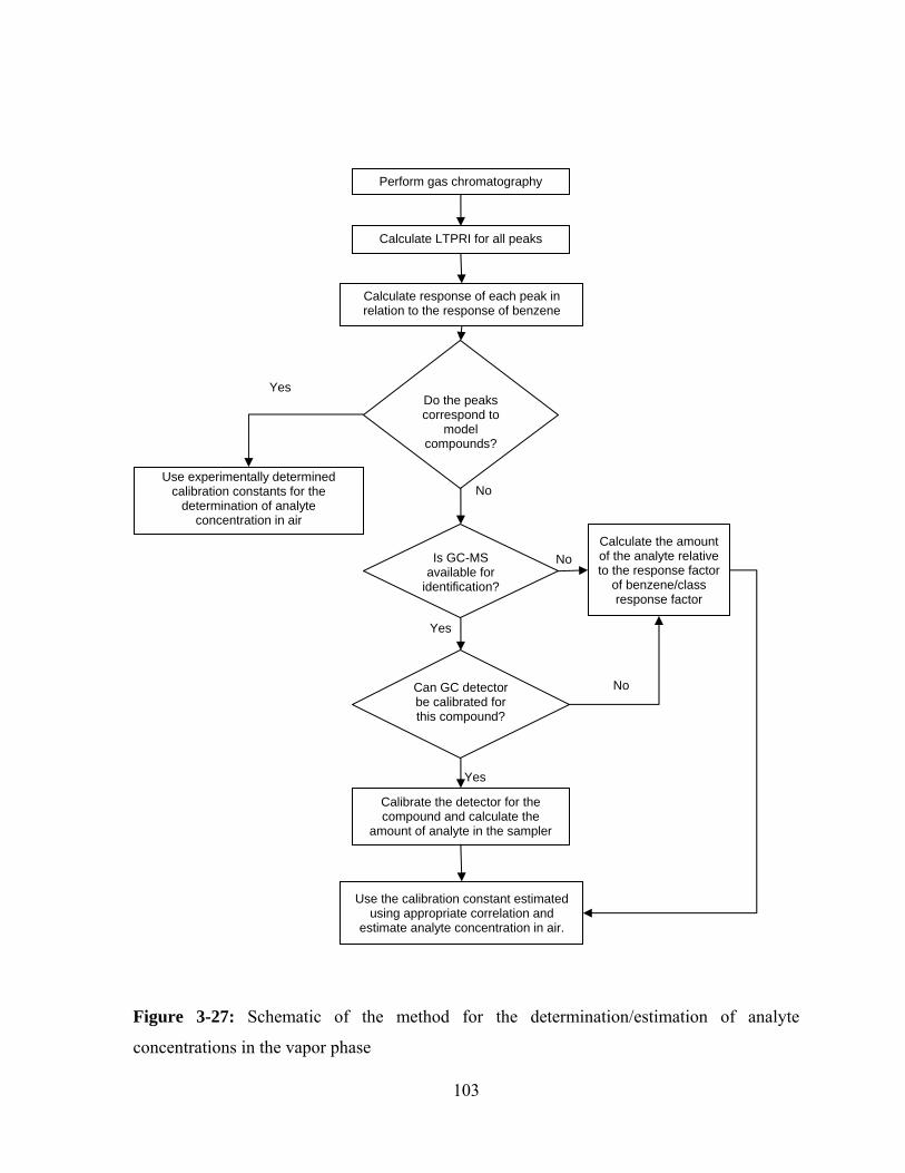
103

Figure 3-27: Schematic of the method for the determination/estimation of analyte

concentrations in the vapor phase

Perform gas chromatography

Calculate LTPRI for all peaks

Calculate response of each peak in relation to the response of benzene

Do the peaks correspond to

model compounds?

Use experimentally determined calibration constants for the

determination of analyte concentration in air

Is GC-MS available for

identification?

Calculate the amount of the analyte relative to the response factor

of benzene/class response factor

Can GC detector be calibrated for this compound?

Calibrate the detector for the compound and calculate the

amount of analyte in the sampler

Use the calibration constant estimated using appropriate correlation and

estimate analyte concentration in air.

Yes

No

No

No

Yes

Yes

104

Using the estimated calibration constant based on the overall correlation between ln(k) and

LTPRI, combined with the use of FID as a detector for GC, can then be a powerful technique

to estimate total parameters such as Total Petroleum Hydrocarbons (TPH) in vapor phase.

Such approach to the determination of TPH is not possible with diffusive-type passive

samplers.

The calibration constants determined in this study have not only enabled the development of

models to estimate calibration constants for unknown compounds, but also allowed the

determination of the permeability of PDMS towards the respective analytes for general use in

analytical techniques based on the use of PDMS. This will be discussed in the next section of

this thesis.

3.5.7 Determination of permeability of PDMS towards VOCs

Experiments reported in this section were conducted under ideal conditions of good air

circulation in the calibration chamber; hence the calibration constants were dependent only

on the permeability of the polymer towards the analytes and the geometry of the membrane.

By definition, the relationship between the calibration constant and permeability (Chapter 2)

is,

PALk m=

Permeabilities of the PDMS membrane towards the 41 model compounds were determined

based on this equation and are provided in Table 3-16. The permeabilities were valid

assuming that the exposed membrane area was equal to the area of the opening of the

sampler’s aluminum crimp cap. The knowledge of PDMS permeability towards various

analytes listed in the table might be valuable for the development of related analytical

techniques (which use analyte permeation through PDMS membranes), such as membrane

inlet mass spectrometry (MIMS) and membrane extraction with a sorbent interface (MESI).

105

Table 3-16: Permeability of PDMS towards various n-alkanes, aromatic hydrocarbons,

alcohols, esters and chlorinated compounds determined based on the relationship between the

calibration constant and permeability.

Compounds P (cm2 min-1)

n-hexane 0.041

n-heptane 0.077

n-octane 0.144

n-nonane 0.265

n-decane 0.428

Benzene 0.076

Toluene 0.149

Ethyl benzene

o-xylene

0.234

0.280

Propyl benzene 0.350

Butyl benzene 0.516

2-methyl-1-propanol 0.040

n-butanol 0.062

2,3-dimethyl-2-butanol 0.058

n-pentanol 0.123

2-hexanol 0.139

2,4-dimethyl-3-pentanol 0.125

n-hexanol 0.229

n-heptanol 0.419

2-octanol 0.461

2-ethyl-1-hexanol 0.493

n-octanol 0.605

2-methyl-1-butanol 0.078

3-octanol 0.264

6-methyl-2-heptanol 0.333

Ethyl acetate 0.042

Propyl acetate 0.080

Methyl butyrate 0.087

sec.butyl acetate 0.081

Ethyl butyrate 0.143

Butyl acetate 0.156

Propyl butyrate 0.248

Butyl butyrate 0.392

1,1- Dichloroethylene 0.026

Dichloromethane 0.038

Cis-1,2-Dichloroethylene 0.060

Chloroform 0.062

1,1,1-Trichloroethane 0.040

1,2-Dichloroethane 0.082

Carbontetrachloride 0.047

Trichloroethylene 0.104

106

3.6 Conclusions

Calibration constants of TWA-PDMS samplers were determined for 41 model compounds

belonging to various chemical classes, including n-alkanes, aromatic hydrocarbons, alcohols,

esters and chlorinated compounds. Reproducibilities of the extraction efficiencies and the

calibration constants were very good. The extraction and the chromatographic method were

free of interferences from compounds extracted with CS2 from the PDMS membrane.

The correlations between ln(k) and LTPRI, as well as ln(k/MW) and LTPRI, were generally

good for all classes except the chlorinated compounds. For the chlorinated compounds,

ln(k/MW) vs. LTPRI was a better model than ln(k) vs. LTPRI. The approach proposed in this

thesis allows easy and fast estimation of the calibration constants of permeation passive

samplers equipped with PDMS membranes. Using LTPRI for the estimation of the

calibration constants comes with the advantage that compound identity need not necessarily

be known at the time of sampling. This is very important, as the decision to sample air or soil

gas does not necessarily come with the knowledge of the identity of the analytes. Once the

identity of the compound is known after the exposure in the field, class-specific correlations

can be used to estimate the calibration constants with better accuracy. Also, the

chromatographic detector can be calibrated for the target compounds once their identity is

established. If not, detectors such as FID, with uniform response towards most organic

compounds, can be utilized for analyte quantification. The results presented in the thesis

should help in broader adoption of permeation passive sampling in different application areas

.

107

CHAPTER 4

Effect of temperature, humidity and linear flow velocity of air on the calibration constants

The three environmental variables which may directly or indirectly affect the uptake rates of

passive samplers are temperature, humidity and air flow patterns around the sampler. In this

chapter, the theoretical aspects and experimental results obtained in calibration experiments

at different temperatures, humidity levels and linear flow velocities of air across the surface

of the sampler will be discussed.

4.1 Theoretical considerations

4.1.1 Effect of temperature

Temperature can play an important role in determining the uptake rate of a sampler

depending on the type of the polymer membrane used as the barrier. Temperature

dependence of polymer permeability towards a given analyte is determined by the

temperature dependences of the diffusion coefficient of the molecule in the polymer, as well

as its partition coefficient between air and the polymer. The partition coefficient and

diffusion coefficient of the molecule, and consequently the permeability of the polymer

towards a particular analyte, can be expressed as a function of temperature using Van’t

Hoff’s and Arrhenius equations:2

(4.1)

(4.2)

(4.3)

(4.4)

⎥⎦

⎤⎢⎣

⎡⎟⎟⎠

⎞⎜⎜⎝

⎛−−=

opo RTRT

EPP 11exp

⎥⎦

⎤⎢⎣

⎡⎟⎟⎠

⎞⎜⎜⎝

⎛−Δ−=

oso RTRT

HKK 11exp

⎥⎦

⎤⎢⎣

⎡⎟⎟⎠

⎞⎜⎜⎝

⎛−−=

odo RTRT

EDD 11exp

( ) ⎥⎦

⎤⎢⎣

⎡⎟⎟⎠

⎞⎜⎜⎝

⎛−Δ+−=

osdoo RTRT

HEKDDK 11exp

108

where Po, Ko and Do are the permeability constant, partition coefficient and diffusion

coefficient at a temperature To, Ep is the activation energy for permeation, ΔHs is the heat of

sorption of the analyte in the membrane, and Ed is the activation energy for diffusion.215

Combining equations (4.1), (4.2) and (4.3), we can express the activation energy of

permeation as:

(4.5)

Equation (4.5) shows that the temperature dependence of permeability is a function of the

analyte’s heat of solution and its activation energy for diffusion. For PDMS, the diffusion

coefficient of a molecule in the polymer increases with increase in temperature, and the

partition coefficient of the molecule decreases with increase in temperature. In other words,

Ed is greater than zero (positive), and ΔHs is less than zero (negative) for most volatile

organic compounds. This observation is in agreement with the permeability characteristics of

PDMS membranes reported by Boscaini et al.188 and Mark et al.216 (among others). Since Ed

and ΔHs oppose each other, there is a trade-off in the net permeability with change in

temperature. This eventually results in the permeability generally being a weak function of

temperature when compared to many other polymers. Further, the net change in the

permeability of the polymer membrane with temperature is decided based on which of these

two parameters defining the activation energy of permeation is dominating.

To understand how the temperature affects the calibration constant, theoretical relationships

between the two parameters were derived as follows.

Equation (4.1) suggests that

(4.6)

From the definition of the calibration constant introduced in Chapter 2 (Equation 2.4), we can

arrive at the relationship as in Eq. (4.7).

(4.7) ( )PA

Lk m lnln)ln( −⎟

⎠⎞

⎜⎝⎛=

o

ppo

RTE

RTE

PP +−= lnln

109

Equations (4.6) and (4.7) can then be used to derive the relationship between temperature and

the calibration constant as in equation (4.8).

(4.8)

According to equation (4.8), a linear relationship should exist between ln(k) and 1/T.

Furthermore, it should be possible to calculate the activation energy of permeation from the

slope of this linear relationship. Experiments can therefore be performed to determine the

calibration constants of the samplers towards various analytes at different temperatures, and

the Ep can be determined from the slope of the ln (k) vs. 1/T line.

4.1.2 Effect of humidity

One of the motivations to use a PDMS membrane as the barrier in the passive sampler is its

low permeability towards water molecules. In the case of diffusive samplers, the uptake rates

of various molecules are determined exclusively by their diffusion coefficients in air. The

diffusion coefficients of water vapour and toluene in air at atmospheric pressure and 25°C are

0.251 cm2s-1 and 0.0827 cm2s-1, respectively.217,218 Consequently, the uptake rate of water for

diffusive-type passive samplers is roughly 3 times higher than that for toluene. On the other

hand, the permeability of toluene in PDMS is approximately 63 times higher than that of

water vapour.212 Accordingly, the uptake rate of water should be only about 0.0157 times that

of toluene when using the TWA-PDMS sampler. Consequently, the chance of the sorbent

getting saturated with water (eventually leading to non-linear sorption of the analyte

molecules) should theoretically be very low when compared to that of diffusive-type passive

samplers. In other words, by using the TWA-PDMS samplers, it should be possible to

prolong the exposure period in humid atmospheres without risking sorbent saturation. This is

particularly valuable when using the samplers for soil gas testing, where the relative humidity

is typically very close to 100%.

4.1.3 Effect of linear flow velocity of air

During the discussion of the theory of the permeation-type passive samplers, it was assumed

that the boundary layer effect is minimal as shown in Figure 2-1. In practice, the boundary

1ln ln ln p pmo

o

E ELk PA RT R T

⎛ ⎞ ⎛ ⎞= − − + ⎜ ⎟⎜ ⎟⎝ ⎠⎝ ⎠

110

layer effect is minimal only when the air velocity around the sampler is sufficiently high.

When the linear flow velocity is below a certain value, a boundary layer will always exist

(Figure 4-1), as the analyte is supplied to the outside surface of the membrane at a rate slower

than the rate at which it is transported into the sampler. The magnitude of this starvation

effect depends on two parameters: the analyte transport rate through the membrane defined

by the permeability of PDMS, and the analyte transport rate within the boundary layer

defined by the diffusion coefficient of the analyte in air. The starvation effect is more

pronounced for compounds for which PDMS permeability is higher because they are

removed from the air near the sampler more rapidly. Since the mass transport across the

boundary layer is generally slower for larger molecules (generally characterized by larger

permeability), the magnitude of the starvation effect usually increases when the size of the

molecule increases.

Figure 4-1: Concentration profile for permeation samplers with starvation effect and with an

ideal sorbent.

In the case of diffusive-type passive samplers, the rate of mass transport of various analytes

through the diffusion barrier decreases with a decrease in their diffusion coefficients.


air

Analyte concentration on the surface of the

membrane


Sample

Membrane thickness

Distance

Con

cent

ratio

n

Boundary layer

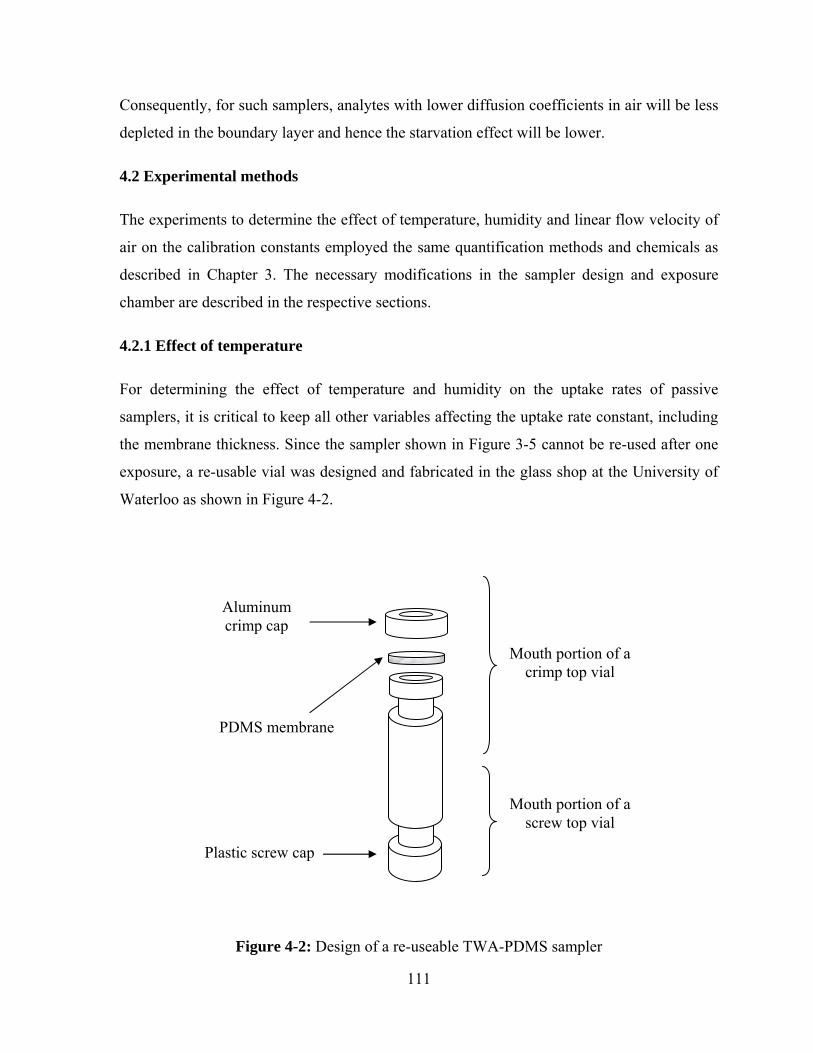
111

Consequently, for such samplers, analytes with lower diffusion coefficients in air will be less

depleted in the boundary layer and hence the starvation effect will be lower.


The experiments to determine the effect of temperature, humidity and linear flow velocity of

air on the calibration constants employed the same quantification methods and chemicals as

described in Chapter 3. The necessary modifications in the sampler design and exposure

chamber are described in the respective sections.


For determining the effect of temperature and humidity on the uptake rates of passive

samplers, it is critical to keep all other variables affecting the uptake rate constant, including

the membrane thickness. Since the sampler shown in Figure 3-5 cannot be re-used after one

exposure, a re-usable vial was designed and fabricated in the glass shop at the University of

Waterloo as shown in Figure 4-2.

Figure 4-2: Design of a re-useable TWA-PDMS sampler

Aluminum crimp cap

PDMS membrane

Mouth portion of a screw top vial

Mouth portion of a crimp top vial

Plastic screw cap

112

The sampler fabrication involved cutting the bottoms of a crimp cap vial and a screw cap vial

(both of same internal and external diameters) and fusing the open vial ends together. This

enabled removing the sorbent from the vials through the screw cap end without disturbing the

membrane, followed by solvent desorption and chromatographic analysis as per the scheme

illustrated in Figure 3-16. Consequently, the sampler design allowed the use of the same set

of 7 samplers for the experiments at different temperatures.

Experiments were performed with three sets of compounds; alkanes and aromatic

hydrocarbons together, linear and branched alcohols together and esters. The list of analytes

is provided in Table 4-1. The experiments were performed at 4 different temperatures

ranging from approximately 10 °C to 40 °C for each set of compounds. These experiments

were conducted at 0% relative humidity, as the effect of humidity on the calibration constants

had not been studied at that time. It was also desired to determine the energy of activation of

permeation without introducing any error related to non-zero humidity (if any). Further, the

fan in the calibration chamber was operated at the maximum speed in order to eliminate any

starvation effects. The average weight of the 7 membranes used for the fabrication of the

samplers was 8.6 mg ± 0.20 mg.

Table 4-1: List of analytes used in the experiments for determining the effect of temperature

on the calibration constant.

Analyte group Analytes

n-alkanes n-hexane, n-heptane, n-octane, n-nonane and n-decane

Aromatic hydrocarbons

Benzene, toluene, ethyl benzene, propyl benzene, and butyl benzene.

Esters Propyl acetate, methyl butyrate, sec-butyl acetate, ethyl butyrate, butyl acetate, propyl butyrate and butyl butyrate.

Linear and branched alcohols

n-butanol, n-pentanol, n-hexanol, n-heptanol, n-octanol, 2-methyl-1-propanol, 2,3-dimethyl-2-butanol, 2-hexanol, 2,4-dimethyl-3-pentanol, 2-octanol, and 2-ethyl-1-hexanol.

113


The experimental setup for the generation of the standard gas mixtures was modified to

produce the desired humidity levels. The modified experimental setup, as shown in Figure 4-

3, involved splitting the dry nitrogen gas prior to its delivery to the exposure chamber into

two streams. One part was saturated with water by bubbling the gas through water in a 2.5

liter glass jar, while the other was passed through the vessel containing the permeation tubes.

The flow rates of the two streams, and hence the humidity at the outlet, could be controlled

using needle valves A and B. The humidity of the resulting standard gas mixture was

measured using a hygrometer (Model 11-661-7D) procured from Fisher Scientific Inc.,

(Ottawa, ON). The experiments performed using the n-alkanes and aromatic hydrocarbons as

the model compounds (see Table 4-1) were carried out at four relative humidity levels:

approximately 0%, 29%, 60% and 91%. The exposure time durations in these experiments

were 4705, 3230, 2997 and 8997 minutes, respectively. The 8997 minutes (6.24 days)

exposure at 91% humidity was carried out to test the performance of the sampler under

“worst case scenario” conditions of high humidity and long exposure duration. The

temperature of the calibration chamber was maintained at 25°C ± 2°C for all the experiments.

Figure 4-3: Schematic representation of the experimental setup used for generating the test

gas atmosphere with the required humidity.

High pressure nitrogen source

Moisture/organic compounds

scrubber

Mass flow controller Permeation

tubes

Water vapour saturated N2

Humidified test gas mixture

Dry N2

A

B

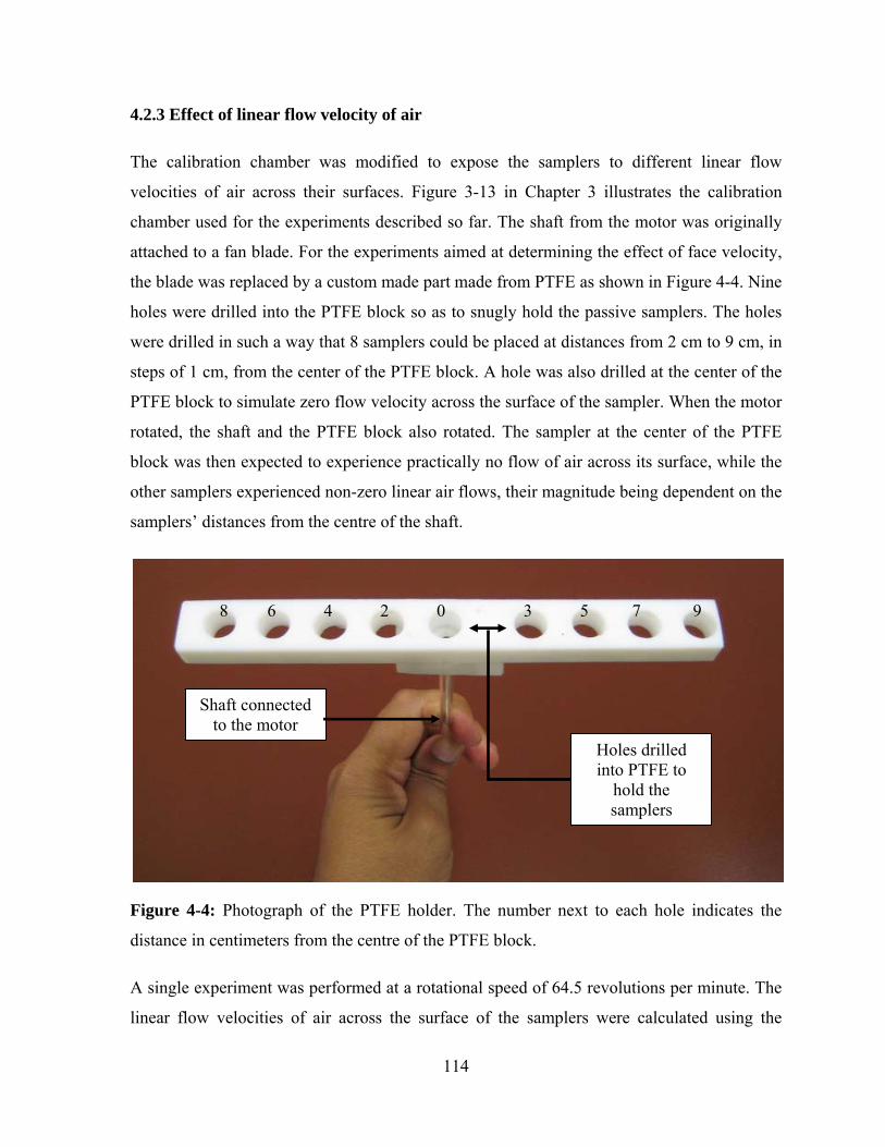
114


The calibration chamber was modified to expose the samplers to different linear flow

velocities of air across their surfaces. Figure 3-13 in Chapter 3 illustrates the calibration

chamber used for the experiments described so far. The shaft from the motor was originally

attached to a fan blade. For the experiments aimed at determining the effect of face velocity,

the blade was replaced by a custom made part made from PTFE as shown in Figure 4-4. Nine

holes were drilled into the PTFE block so as to snugly hold the passive samplers. The holes

were drilled in such a way that 8 samplers could be placed at distances from 2 cm to 9 cm, in

steps of 1 cm, from the center of the PTFE block. A hole was also drilled at the center of the

PTFE block to simulate zero flow velocity across the surface of the sampler. When the motor

rotated, the shaft and the PTFE block also rotated. The sampler at the center of the PTFE

block was then expected to experience practically no flow of air across its surface, while the

other samplers experienced non-zero linear air flows, their magnitude being dependent on the

samplers’ distances from the centre of the shaft.

Figure 4-4: Photograph of the PTFE holder. The number next to each hole indicates the

distance in centimeters from the centre of the PTFE block.

A single experiment was performed at a rotational speed of 64.5 revolutions per minute. The

linear flow velocities of air across the surface of the samplers were calculated using the

Shaft connected to the motor

Holes drilled into PTFE to

hold the samplers

8 6 4 2 0 3 5 7 9

115

circumference covered by each sampler. The experiments were performed at 25°C ± 2°C,

and 0% relative humidity. The analytes used for this study were n-alkanes and aromatic

hydrocarbons listed in Table 4-1.


The results obtained from the experiments allowed the determination of the fundamental

transport properties of PDMS (energy of activation of permeation) towards the model

compounds used in the study and provided critical information on the variability of the

calibration constants with temperature, humidity and linear flow velocity of air that should be

carefully considered during field deployment of the samplers. The results are discussed in the

next three sub-sections.


The calibration constants of n-alkanes and aromatic hydrocarbons determined at 10°C,

19.7°C, 29.9°C and 39.5°C are listed in Table 4-2. The calibration constants increased with

increase in temperature in all cases. By definition, the calibration constant is inversely

proportional to the permeability of PDMS towards an analyte. Consequently, the

experimental results indicated that the permeability decreased with increase in temperature.

This is in agreement with many observations on the permeability of PDMS as a function of

temperature, as discussed in the theory section. A plot of 1/T vs ln(k) for each of the n-

alkanes and aromatic hydrocarbons, as shown in Figures 4-5 and 4-6, reiterated the earlier

observations noted in the literature that the permeability is related to temperature through

Arrhenius-type relationships for PDMS. The correlation was good for all the analytes

studied, with the correlation coefficients ranging from 0.9082 for n-hexane to 0.9990 for

propyl benzene.

The slopes of the correlations were used to determine the energy of activation of permeation

(using equation 4.8) and are listed in Table 4-3 along with the standard error of the slope.

The energy of activation of permeation was negative, which shows that the heat of solution

(ΔHs) of the analytes in PDMS was the dominating factor when compared with the energy of

activation of diffusion (Ed) within the polymer (refer to equation 4.5). Within the n-alkanes

116

homologous series, the Ep values decreased from -8 kJ mole-1 for n-hexane to -13 kJ.mole-1

for n-nonane, and then increased again to -7 kJ.mole-1 for n-decane. A similar trend within

the aromatic hydrocarbons was noticed where the Ep decreased from -8 kJ mole-1 for benzene

to -11 kJ mole-1 for ethyl benzene, and increased again to -5 kJ mole-1 for butyl benzene. Nevertheless, the Ep values were all within the same order of magnitude, as has been

observed by other researchers.188

For n-hexane, the increase in temperature from 10°C to 39.5°C resulted in the uptake rate

decreasing from 1.24 mL/min to 0.9 mL/min, a decrease of 27.3% in the uptake rate. This

corresponds to an average decrease in the uptake rate of about 0.9% per °C change within the

temperature range studied. Within the n-alkanes group, n-octane had the highest average

percentage decrease of 1.4% in the uptake rate per °C increase in temperature.

Mathematically, the closer the energy of activation of permeation is to zero, the smaller is the

effect of a change in temperature on the calibration constant.

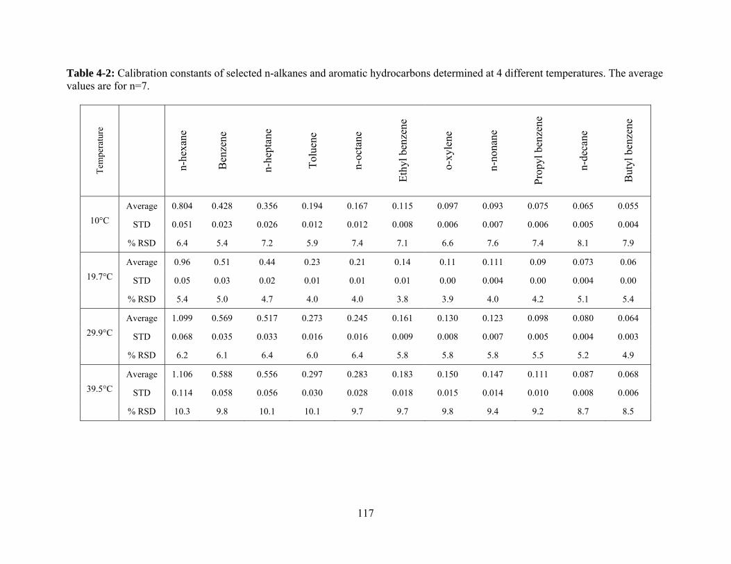
117

Table 4-2: Calibration constants of selected n-alkanes and aromatic hydrocarbons determined at 4 different temperatures. The average values are for n=7.

Tem

pera

ture

n-he

xane

Ben

zene

n-he

ptan

e

Tolu

ene

n-oc

tane

Ethy

l ben

zene

o-xy

lene

n-no

nane

Prop

yl b

enze

ne

n-de

cane

But

yl b

enze

ne

Average 0.804 0.428 0.356 0.194 0.167 0.115 0.097 0.093 0.075 0.065 0.055 10°C STD 0.051 0.023 0.026 0.012 0.012 0.008 0.006 0.007 0.006 0.005 0.004

% RSD 6.4 5.4 7.2 5.9 7.4 7.1 6.6 7.6 7.4 8.1 7.9 Average 0.96 0.51 0.44 0.23 0.21 0.14 0.11 0.111 0.09 0.073 0.06

19.7°C STD 0.05 0.03 0.02 0.01 0.01 0.01 0.00 0.004 0.00 0.004 0.00 % RSD 5.4 5.0 4.7 4.0 4.0 3.8 3.9 4.0 4.2 5.1 5.4 Average 1.099 0.569 0.517 0.273 0.245 0.161 0.130 0.123 0.098 0.080 0.064

29.9°C STD 0.068 0.035 0.033 0.016 0.016 0.009 0.008 0.007 0.005 0.004 0.003 % RSD 6.2 6.1 6.4 6.0 6.4 5.8 5.8 5.8 5.5 5.2 4.9 Average 1.106 0.588 0.556 0.297 0.283 0.183 0.150 0.147 0.111 0.087 0.068

39.5°C STD 0.114 0.058 0.056 0.030 0.028 0.018 0.015 0.014 0.010 0.008 0.006 % RSD 10.3 9.8 10.1 10.1 9.7 9.7 9.8 9.4 9.2 8.7 8.5

118

Figure 4-5: Arrhenius-type relationship between ln(k) and 1/T for n-alkanes.

Figure 4-6: Arrhenius-type relationship between ln(k) and 1/T for aromatic hydrocarbons.

R² = 0.9082

R² = 0.9721

R² = 0.9964

R² = 0.9842

R² = 0.9985

-3.5

-3.0

-2.5

-2.0

-1.5

-1.0

-0.5

0.0

0.5

0.00305 0.00315 0.00325 0.00335 0.00345 0.00355

ln (k

)

1/T

n-alkanes - dependence of the calibration constants on temperature

n-Hexane

n-Heptane

n-Octane

n-nonane

n-decane

R² = 0.9431

R² = 0.9833

R² = 0.9985

R² = 0.9970

R² = 0.9990

R² = 0.9960

-3.3

-2.8

-2.3

-1.8

-1.3

-0.8

-0.3

0.0031 0.0032 0.0033 0.0034 0.0035 0.0036

ln (k

)

1/T

Aromatic hydrocarbons - dependence of the calibration constants on temperature

Benzene

Toluene

Ethyl benzene

o-Xylene

Propyl benzene

Butyl benzene

119

Table 4-3: Energy of activation of permeation for selected n-alkanes and aromatic

hydrocarbons determined using the slope of the Arrhenius-type plots shown in Figures 4-5

and 4-6.

Compound Slope ×10-3Standard error of the slope ×

10-2 Ep

(kJ mole-1) R2 for the ln(k) vs. 1/T correlation

n-hexane -1 2.2 -8 0.9082

n-heptane -1.3 1.6 -11 0.9721

n-octane -1.6 1 -13 0.9964

n-nonane -1.3 1.2 -11 0.9842

n-decane -1 0 -7 0.9985

Benzene -1 1.7 -8 0.9431

Toluene -1.3 1.2 -11 0.9833

Ethyl benzene -1.3 0 -11 0.9985

Propyl benzene -1.2 0 -9.7 0.9990

Butyl benzene -1 0 -5 0.9960

o-xylene -1.3 0 -11 0.9970

A similar trend of increasing calibration constants with increase in temperature (Table 4-4)

was also observed for all esters. The linearity of the ln(k) vs. LTPRI curve was good for 5 out

of the 7 compounds studied with the correlation coefficient greater than 0.98, as shown in

Figure 4-7. The correlation for propyl butyrate and butyl butyrate deviated from the straight

line, which could partially be attributed to their high uptake rates and consequently higher

starvation effect despite the best efforts to have proper air circulation inside the calibration

chamber. A slight deviation from linearity was observed for sec-butyl acetate, but the

120

correlation coefficient (0.9869) was not as bad as that for propyl butyrate and butyl butyrate.

The energy of activation of permeation for all the esters was calculated (Table 4-5). The

values were generally lower than those observed for the n-alkanes and aromatic

hydrocarbons.

Table 4-4: Calibration constants of selected esters determined at 4 different temperatures.

The average values are for n=7.

Tem

pera

ture

Prop

yl a

ceta

te

Met

hyl b

utyr

ate

Sec-

buty

l ace

tate

Ethy

l but

yrat

e

But

yl a

ceta

te

Prop

yl b

utyr

ate

But

yl b

utyr

ate

Average 0.199 0.186 0.205 0.135 0.129 0.108 0.096

12°C STD 0.022 0.020 0.023 0.013 0.012 0.010 0.010

% RSD 10.8 10.7 11.2 9.8 9.7 8.8 10.0

Average 0.232 0.217 0.236 0.153 0.144 0.115 0.099

20°C STD 0.026 0.024 0.027 0.016 0.015 0.011 0.009

% RSD 11.1 10.9 11.4 10.3 10.3 9.5 9.0

Average 0.28 0.26 0.29 0.18 0.17 0.13 0.10

30.5°C STD 0.03 0.02 0.03 0.02 0.01 0.01 0.01

% RSD 9.2 9.1 9.6 8.5 8.4 7.7 7.2

Average 0.326 0.302 0.367 0.209 0.198 0.155 0.120

39.5°C STD 0.034 0.031 0.041 0.021 0.019 0.014 0.011

% RSD 10.5 10.4 11.2 9.9 9.8 9.1 8.8

121

Figure 4-7: Arrhenius-type relationship between ln(k) and 1/T for esters.

Table 4-5: Energy of activation of permeation for selected esters determined using the slope

of the Arrhenius-type plots shown in Figure 4-7.

Compound Slope ×10-3

Standard error of the slope × 10-2

Ep (kJ mole-1) R2 for the ln(k) vs.

1/T correlation

Propyl acetate -1.8 1 -15 0.9971

Methyl butyrate -1.8 1 -15 0.998

Sec-butyl acetate -2.1 1.7 -17 0.9869

Ethyl butyrate -1.6 1 -14 0.994

Butyl acetate -1.6 1.1 -13 0.9911

Propyl butyrate -1.4 2.5 -11 0.9390

Butyl butyrate -1 2.8 -7 0.8269

The alcohols also revealed an increasing trend in the calibration constants with temperature

(Table 4-6). As shown in Figures 4-8 and 4-9, the 1/T vs. ln(k) plots showed generally good

R² = 0.9971R² = 0.998

R² = 0.9869

R² = 0.994R² = 0.9911

R² = 0.939

R² = 0.8269

-2.5

-2.3

-2.1

-1.9

-1.7

-1.5

-1.3

-1.1

-0.9

0.0031 0.0032 0.0032 0.0033 0.0033 0.0034 0.0034 0.0035 0.0035 0.0036

ln (k

)

1/T

Esters - dependence of the calibration constants on temperature

Propyl acetate

Methyl butyrate

sec. butyl acetate

Ethyl butyrate

Butyl acetate

Propyl butyrate

Butyl butyrate

122

correlations for all compounds except for 2,3-dimethyl-2-butanol (r2 = 0.6967) and n-octanol

(r2 = 0.8294). Within the n-alcohols group, there was also a similar trend of increasing energy

of activation of permeation from -13 kJ mole-1 for n-butanol to -8 kJ mole-1 for n-heptanol,

followed by a reversal in the trend with -9.3 kJ mole-1 for n-octanol.

From the results observed for all the different groups of compounds and from the literature

data it can be concluded that for most VOCs, the energy of activation of permeation through

PDMS is indeed mainly governed by the heat of solution of the analyte in the membrane, and

to a much smaller extent by the energy of activation of diffusion. Furthermore, the results

also indicate that the energy of activation of permeation is mostly of the same order of

magnitude for all the compounds irrespective of their polarities.

The temperature variations of the uptake rates observed for the model compounds studied in

this project were somewhat higher than the theoretically calculated ~0.4% per degree Celsius

change for diffusive-type passive samplers reported in the literature.219 It should be noted that

when the temperature increases, the uptake rates should increase for diffusive-type passive

samplers, while they decrease for the sampler designed in this project. In practice, the

diffusive-type passive samplers have been reported to be dependent on temperature to

various degrees by different researchers. For example, Penniquin-Cardinal et al. found that

the uptake rate decreased by 0.6%/°C for benzene, while it increased by 0.35%/°C for

toluene and 0.5%/°C for ethyl benzene and xylenes for the diffusive-type Radiello®

samplers.220 Piechocki-Minguy et al. observed an average 2%/°C change in the uptake rate of

nitrogen dioxide between 5°C and 30°C using their custom-made diffusive-type passive

sampler.221 The variations in the uptake rates with temperature for the TWA-PDMS samplers

are still relatively small compared to other sources of variability under field conditions, such

as linear flow velocity of air across the sampler (discussed in the next section), temporal

concentration variations, etc. Furthermore, for typical applications in indoor air and soil gas

analysis, the temperature of the air is usually nearly constant. Consequently, temperature

variations are expected to play only a minimal role in field applications. When more accurate

results are desired, appropriate corrections to the calibration constants can be made based on

the knowledge of temperature variations in the field.

123

Table 4-6: Calibration constants of selected n-alcohols and branched alcohols determined at 4 different temperatures.

Temperature

2-m

ethy

l-1-

prop

anol

n-bu

tano

l

2,3-

dim

ethy

l-2-

buta

nol

n-pe

ntan

ol

2-he

xano

l

2,4-

dim

ethy

l-3-

pent

anol

n-he

xano

l

n-he

ptan

ol

2-oc

tano

l

2-et

hyl-1

-he

xano

l

n-oc

tano

l

Average 0.391 0.282 0.182 0.14 0.119 0.111 0.074 0.052 0.043 0.050 0.046

10°C STD 0.018 0.018 0.006 0.01 0.007 0.004 0.004 0.002 0.003 0.002 0.002

% RSD 4.6 6.5 3.1 5.8 5.9 3.9 4.8 3.2 6.5 4.0 3.8

Average 0.455 0.338 0.209 0.165 0.14 0.128 0.087 0.059 0.049 0.057 0.046

20.1°C STD 0.012 0.008 0.003 0.004 0.00 0.004 0.004 0.003 0.005 0.004 0.003

% RSD 2.7 2.3 1.6 2.5 2.9 3.0 4.0 4.5 10.0 7.5 6.7

Average 0.465 0.358 0.195 0.175 0.188 0.130 0.094 0.062 0.053 0.060 0.047

29.9°C STD 0.009 0.013 0.004 0.005 0.005 0.003 0.002 0.001 0.004 0.002 0.001

% RSD 1.9 3.6 2.0 3.1 2.5 2.1 2.3 2.2 8.4 2.8 2.5

Average 0.611 0.491 0.233 0.226 0.194 0.148 0.112 0.074 0.066 0.076 0.052

40.1°C STD 0.019 0.020 0.007 0.007 0.01 0.004 0.002 0.002 0.01 0.003 0.002

% RSD 3.2 4.1 2.9 2.9 3.1 2.8 2.2 2.2 7.6 3.6 3.1

124

Figure 4-8: Arrhenius-type relationship between ln(k) and 1/T for n-alcohols.

Figure 4-9: Arrhenius-type relationship between ln(k) and 1/T for branched alcohols.

R² = 0.9342

R² = 0.9538

R² = 0.988R² = 0.9679

R² = 0.8294

-4.0

-3.5

-3.0

-2.5

-2.0

-1.5

-1.0

-0.5

0.0

0.00315 0.0032 0.00325 0.0033 0.00335 0.0034 0.00345 0.0035 0.00355

ln (k

)

1/T

n-alcohols - dependence of the calibration constants on temperature

n-butanol

n-pentanol

n-hexanol

n-heptanol

n-octanol

R² = 0.9042

R² = 0.6967

R² = 0.9485

R² = 0.9459R² = 0.9628

-3.5

-3.0

-2.5

-2.0

-1.5

-1.0

-0.5

0.0

0.00315 0.00325 0.00335 0.00345 0.00355

ln (k

)

1/T

Branched alcohols - Dependence of calibration constant on temperature

2-methyl-1-propanol

2,3-dimethyl-2-butanol

2,4-dimethyl-3-pentanol

2-ethyl-1-hexanol

2-octanol

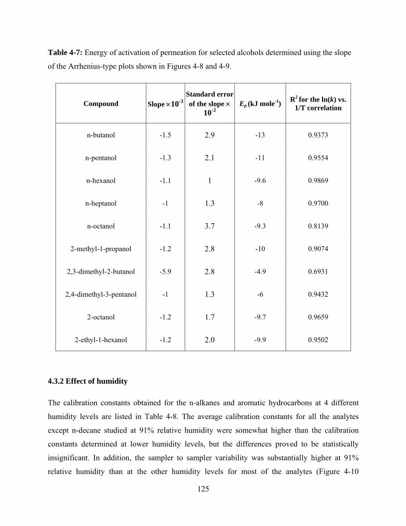
125

Table 4-7: Energy of activation of permeation for selected alcohols determined using the slope

of the Arrhenius-type plots shown in Figures 4-8 and 4-9.

Compound Slope ×10-3Standard error of the slope ×

10-2 Ep

(kJ mole-1) R2 for the ln(k) vs. 1/T correlation

n-butanol -1.5 2.9 -13 0.9373

n-pentanol -1.3 2.1 -11 0.9554

n-hexanol -1.1 1 -9.6 0.9869

n-heptanol -1 1.3 -8 0.9700

n-octanol -1.1 3.7 -9.3 0.8139

2-methyl-1-propanol -1.2 2.8 -10 0.9074

2,3-dimethyl-2-butanol -5.9 2.8 -4.9 0.6931

2,4-dimethyl-3-pentanol -1 1.3 -6 0.9432

2-octanol -1.2 1.7 -9.7 0.9659

2-ethyl-1-hexanol -1.2 2.0 -9.9 0.9502


The calibration constants obtained for the n-alkanes and aromatic hydrocarbons at 4 different

humidity levels are listed in Table 4-8. The average calibration constants for all the analytes

except n-decane studied at 91% relative humidity were somewhat higher than the calibration

constants determined at lower humidity levels, but the differences proved to be statistically

insignificant. In addition, the sampler to sampler variability was substantially higher at 91%

relative humidity than at the other humidity levels for most of the analytes (Figure 4-10

126

illustrates this for n-hexane). This can be attributed to higher variability in the extraction

efficiencies of the various analytes in the presence of different quantities of water in the sorbent.

Such a phenomenon was noticed by Sunesson and co-workers when trying to desorb analytes

from Anasorb 747® with thermal desorption methods.222 A potential solution for reducing the

variability would be to use a co-solvent for desorption, such as isopropyl alcohol, to enable

partial miscibility of the traces of water which permeated through the PDMS membrane with the

extraction solvent. Overall, the uptake rates were within 12.5% RSD for all the analytes when

determined at the four different temperatures, which can be considered insignificant when

compared to other uncertainties in measurement under field conditions.

The fact that the calibration constants change very little at different humidity levels is very

advantageous when using the TWA-PDMS sampler for soil gas sampling applications, as the

humidity in such matrices is often close to 100%. Further, the samplers can be deployed for a

longer time than diffusive samplers (to reduce the limits of detection and quantification), as the

saturation of the sorbent by moisture does not occur as early as it does for the latter.

127

Table 4-8: Calibration constants of selected n-alkanes and aromatic hydrocarbons determined at 4 different humidity levels.

Humidity

n-he

xane

Ben

zene

n-he

ptan

e

Tolu

ene

n-oc

tane

Ethy

l be

nzen

e

n-no

nane

o-xy

lene

Prop

yl

benz

ene

n-de

cane

But

yl

benz

ene

Ave. 0.624 0.343 0.299 0.171 0.154 0.109 0.097 0.096 0.079 0.074 0.063 0% STD 0.046 0.025 0.022 0.013 0.011 0.009 0.008 0.007 0.006 0.006 0.005

%RSD 7.5 7.3 7.4 7.4 6.9 7.9 8.2 7.8 8.1 8.1 7.8

Ave. 0.591 0.316 0.27 0.153 0.136 0.096 0.083 0.081 0.067 0.062 0.053 29% STD 0.04 0.018 0.017 0.009 0.008 0.006 0.007 0.006 0.006 0.007 0.006

%RSD 6.7 5.8 6.1 5.9 6.1 6.8 8 7.4 8.7 10.7 11.3

Ave. 0.611 0.329 0.275 0.158 0.133 0.096 0.080 0.081 0.065 0.059 0.050 60% STD 0.024 0.012 0.011 0.006 0.006 0.005 0.005 0.004 0.004 0.005 0.004

%RSD 3.9 3.6 3.9 3.8 4.4 5.1 6.6 5.1 6.7 8.1 8.1

Ave. 0.643 0.354 0.306 0.168 0.145 0.104 0.081 0.083 0.065 0.057 0.048 91% STD 0.084 0.055 0.047 0.022 0.022 0.013 0.01 0.011 0.007 0.005 0.004

%RSD 13.1 15.5 15.2 13.2 14.9 12.8 11.8 13.5 11.3 8.1 7.9

Average k 0.617 0.336 0.288 0.163 0.142 0.101 0.085 0.085 0.069 0.063 0.054

% RSD 3.5 4.9 6.1 5.2 6.7 6.3 9.3 8.5 9.8 12.1 12.4

128

Figure 4-10: Variation of the calibration constants for n-hexane with changes in humidity.

The error bars correspond to one standard deviation of the mean, and the dotted line indicates

the average calibration constant.


Of all the environmental parameters that have been discussed in this chapter, the effect of

linear flow velocity of air on the uptake rates is perhaps the most important. It should be

noted here that while calculating the linear flow velocity of air experienced by each sampler,

it was assumed that the air was stationary in the calibration chamber, and the rotation of the

sampler alone contributed to the relative flow of air across the face of the sampler. This was

not necessarily true, since the rotating component could drag the air and the samplers could

therefore experience a linear flow velocity lower than the calculated rotational speed (except

for the sampler positioned in the axis of rotation, which may have experienced some flow

across the face via turbulence). Further, since there was a flow of 1000 ml/min of the

standard test gas mixture through the chamber, there was bound to be some movement of air,

which could contribute to errors in the calculation of the linear flow velocity of air across the

surface of the sampler.

The uptake rate of the sampler is proportional to the ratio of the peak area (obtained from

injecting the CS2 extract of the sorbent in the sampler) to exposure duration (M/t). These

0 10 20 30 40 50 60 70 80 90 100.30

.40

.50

.60

.70

.80

.90

1.00

% Relative humidity

calib

ratio

n co

nsta

nt

129

ratios for all the n-alkanes and aromatic hydrocarbons studied are tabulated for estimated

linear air flow velocities from 0 m/s to 0.53 m/s in Table 4-9. In all cases, as expected, the

uptake rate decreased somewhat when the air flow velocity approached 0 m/s. This can be

attributed to the starvation effect discussed in Chapter 2. As the linear flow velocity

increased, the starvation effect decreased, and the uptake rates stabilized at around 0.35 m/s

for all the analytes. A plot of the peak area/exposure duration ratio against linear flow

velocity for n-hexane and butyl benzene is shown in Figures 4-11 and 4-12, respectively. The

uptake tended to reach a plateau at around 0.35 m/s. This is close to the 0.4 m/s reported by

Cinnau for diffusive-type passive samplers.223

The magnitude of the percentage decrease in the uptake rate between the maximum flow

velocity of 0.53 m/s and 0 m/s increased from n-hexane (39.7%) to butyl benzene (47.2%).

As discussed earlier, the starvation effect is a function of the permeability (increased

permeability leads to decreased availability of the analytes around the sampler), as well as

the diffusion coefficient of the analyte in the boundary layer (smaller diffusion coefficient

results in slower mass transfer through the boundary layer). Since the permeability of PDMS

increases from n-hexane to butyl benzene, the starvation effect component due to

permeability also increases in the same direction. In addition, the diffusion coefficient

decreases from n-hexane to butyl benzene, which further worsens the net starvation effect by

reducing the mass transport rate through the boundary layer. The results obtained, showing

increasingly stronger starvation effect from n-hexane to butyl benzene (Table 4-9), were

therefore in accordance with the theoretical predictions.

130

Table 4-9: Variation in the ratio of the peak area to exposure duration (proportional to uptake rates) of TWA-PDMS samplers towards various analytes at linear flow velocities from 0 to 0.53 m/s.

Analyte

Linear flow velocity of air (m/s) % Decrease in

uptake rate with change from 0.53

to 0 m/s 0.00 0.12 0.18 0.23 0.29 0.35 0.41 0.47 0.53

n-hexane 214 223 230 283 311 332 345 339 355 39.7

Benzene 489 520 530 646 708 748 792 776 807 39.4

n-heptane 229 252 255 309 337 358 381 374 382 40.0

Toluene 591 661 677 811 884 936 1008 983 991 40.4

n-octane 211 243 255 300 323 345 376 363 365 42.1

Ethyl benzene 352 408 435 507 543 584 635 609 610 42.3

o-xylene 245 288 310 358 387 414 453 432 432 43.1

n-nonane 155 187 207 235 248 271 297 281 281 44.8

Propyl benzene 194 233 262 295 312 340 374 350 352 44.9

n-decane 124 154 180 196 204 225 251 231 233 46.9

Butyl benzene 119 148 175 190 198 218 244 222 226 47.2

131

Figure 4-11: The effect of linear flow velocity of air on the uptake rate of n-hexane.

Figure 4-12: The effect of linear flow velocity of air on the uptake rate of butyl benzene.

In practice, the effect of linear flow velocity of air should always be considered in the context

of the particular application of the TWA-PDMS samplers. In outdoor air sampling, the linear

flow velocity of air is about 4 m/s on average, while for indoor air in well-ventilated

buildings it is likely to be above 0.35 m/s in most cases. Consequently, the effect of face

050

100150200250300350400

0 0.1 0.2 0.3 0.4 0.5 0.6

Peak

are

a/m

inut

e ex

posu

re

Linear flow velocity m/sec

n-hexane

0

50

100

150

200

250

300

0 0.1 0.2 0.3 0.4 0.5 0.6

Peak

are

a/m

inut

e ex

posu

re

Linear flow velocity m/sec

Butyl benzene

132

velocity can be ignored in these cases. However, when using the TWA-PDMS samplers for

soil gas sampling, with the samplers deployed inside sealed boreholes, the linear flow

velocity of air across the surface of the sampler is essentially zero. Consequently, the

starvation effect has to be taken into account when interpreting the data generated.

4.4 Conclusions

It is important to consider the effect of environmental factors on the uptake rates of any

passive sampler for accurate determination of the analyte concentrations in the gas phase.

The TWA-PDMS sampler has very significant advantages when considering the effects of

humidity on the calibration constant or when considering the deployment duration of the

sampler in the field. This is true because of the low permeability of PDMS towards water

vapor. The negligible effect of humidity on the analyte uptake has been experimentally

demonstrated by performing experiments at different humidity levels.

Increase in temperature results in decreased uptake rates for TWA-PDMS samplers, while it

results in an increase in the uptake rates for diffusive-type passive samplers. The magnitude

of the difference is slightly higher for the TWA-PDMS samplers, but can be considered

negligible when averaging the temperature over a 24 hour period or multiples of 24 hours.

The experiments performed to determine the variation in the calibration constants with

temperature allowed the determination of the energy of activation of permeation of various

analytes through PDMS.

Linear flow velocity of air can have a significant effect on the uptake rates of TWA-PDMS

samplers when it is below 0.35 m/s. A similar effect has been observed for diffusive-type

passive samplers. The difference in the uptake rates between that obtained at 0 m/s and the

0.53 m/s linear flow velocity was found to increase with the increase in the mass transport

rate of the analyte within the membrane. The effect of face velocity can therefore be

disadvantageous for soil gas applications, while it can mostly be ignored for indoor (with

forced ventilation) and outdoor air analysis because of constant air movement.

133

CHAPTER 5

Effect of membrane geometry and exposure duration on the calibration

constants for various analytes

The objective of this chapter is to show how the membrane geometry (thickness and surface

area exposed to the sample matrix) and the sampler exposure duration affect the uptake rates

of the TWA-PDMS sampler.

As discussed in the theory section of this thesis, the calibration constants of the sampler

towards various analytes are functions of the thickness and the area of the membrane exposed

to the sample matrix. According to Fick’s laws, the uptake rate is directly proportional to the

area of the membrane exposed to the sample matrix and inversely proportional to the

thickness of the membrane. Apart from changes in the uptake rates, it should also be noted

that the starvation effect should in principle be lower if the mass transport across the

membrane is reduced either by increasing the membrane thickness, or by reducing the area of

the membrane exposed to the sample. Increasing the membrane exposure area or reducing the

membrane thickness, on the other hand, should aid in lowering the limits of detection and

limits of quantification of the analytical procedure.

Three different thicknesses of PDMS membranes were used to study the effect of the

membrane thickness on the calibration constants of the sampler towards various analytes.

The sampler design discussed in Chapter 3 and all the experiments up to this point used the

1.8 mL crimp cap, autosampler vials. Vials and crimpers of other sizes are available

commercially and can also be used to increase or decrease the membrane area exposed to the

sample matrix. Samplers fabricated using vials of 0.8 and 1.8 mL volume were used to

perform head-to-head comparisons of two different areas of the membrane exposed to the

sample matrix.

Exposure duration and analyte concentrations have been reported to have substantial effects

on the uptake kinetics of diffusive-type passive samplers (also discussed in Section 1.7.4).

Both these parameters influence the uptake rate mainly because of non-ideal functioning of

the sorbent used in the fabrication of the respective diffusive-type passive samplers. The non-

134

ideality arises because of premature saturation of the sorbent and/or competition for the

adsorptive sites by water molecules over time. Since PDMS has low permeability towards

water vapor compared to the compounds of interest, competition by water molecules should

in principle be vastly reduced or eliminated altogether. Consequently, the sampler presented

in this thesis should be able to function properly for a long time without changes of the

uptake rates.

Separate experiments were not performed to determine the effects of exposure duration on

the uptake rates, as sufficient information was available from earlier experiments. The uptake

rates determined for n-hexane over the last 4 years using different exposure durations will be

presented here.


In this section, the experimental methods used for the determination of the effect of the

membrane thickness, exposure area and sampling duration on the calibration constant of the

sampler towards various analytes are described. These experimental methods were in general

the same as described in Chapter 3, except as noted below in the respective sub-sections. The

calibration constants were determined in the same manner as described earlier. The speed of

rotation of the fan blades in the exposure chamber was kept high to minimize the starvation

effect. The experiments were conducted at 0% relative humidity and at 25 ± 2˚C.

5.1.1 Effect of membrane thickness

The experimental study on the effect of membrane thickness on the calibration constant of

the sampler towards various analytes was carried out prior to most of the experimental

studies reported in this thesis. The analytes used for the experiments were n-alkanes from

hexane to decane, benzene, toluene, ethyl benzene, propyl benzene and butyl benzene. In

total, nine vials were deployed in the calibration chamber, among which three had 25 μm

thick membranes, three had 75 μm thick membranes and three had 150 μm thick membranes

procured from Specialty Silicone Products Inc., (Ballston Spa, NY). The membrane thickness

was specified by the manufacturer with a tolerance of ±20%. The analyte concentrations

135

ranged between 279 µg/m3 and 3438 µg/m3 in the exposure chamber, and the total exposure

duration was 8929 minutes.

5.1.2 Effect of membrane area

To determine the effect of membrane area, four 0.8 mL crimp cap vials (with an exposure

area of 11.5 mm2) and three 1.8 mL crimp cap vial (with an exposure area of 21.4 mm2) were

exposed in the chamber to n-alkanes (from hexane to decane) and aromatic hydrocarbons

(benzene, toluene, ethyl benzene, propyl benzene and butyl benzene) at concentrations

ranging from 41 µg/m3 to 1025 µg/m3 for a duration of 8715 minutes. The nominal

membrane thickness used was 75 µm ±20% and the membranes required for all the samplers

were cut from an area of 2” x 2” from the PDMS sheet procured from the manufacturer.

5.1.3 Effect of exposure duration

Over a period of time, a number of exposure experiments were performed for the

determination of the calibration constants of the 40 compounds listed in Chapter 3. The

permeation tube design and the specifications of the PTFE tubing used for the fabrication of

the permeation tubes were the same in all these experiments. Since the permeation rates of

the different analytes through PTFE were different (resulting in different concentrations of

the analytes in the chamber), many trial and error experiments were conducted by changing

the sampler exposure duration (in addition to changing the permeation tube temperature and

length) in order to trap enough analytes in the sampler for quantification by the

chromatographic method. The experiments were challenging as the sensitivity of different

chromatographic detectors (FID, ECD) and the injection systems available on the instruments

used for the analysis (cool on-column and split-splitless) were different. In-order to control

the calibration chamber performance, n-hexane was sometimes used along with the

respective sets of model compounds while determining the calibration constants. Some of the

selected exposures of different duration at the same (or very close) n-hexane concentrations

are discussed here. The concentrations of n-hexane ranged from 605 µg/m3 to 923 µg/m3 and

the exposure duration ranged from 1 day to 9 days.

136


The results obtained from the experiments described above provided important information

on the parameters that have to be carefully assessed for future optimization of the uptake rate

and sampler deployment duration in the field. For a specific concentration of the analytes in

the sample matrix, the membrane geometry and exposure duration define the detection and

quantification limits of the sampler towards the respective analytes. The observations and

interpretations from these experiments are provided in the next three subsections.

5.2.1 Effect of membrane thickness

The calibration constants obtained for the test of different membrane thicknesses are given in

Table 5-1. Samplers coded PS-1, PS-2 and PS-3 had 25 μm membranes; those coded PS-4,

PS-5 and PS-6 had 75 μm membranes, and the ones coded PS-7, PS-8 and PS-9 had 150 μm

membranes. The calibration constants should theoretically be linearly proportional to the

inverse of the membrane thickness. The calibration constants for the samplers equipped with

the 25 μm thick membranes were 25 to 50 % lower than those for the 75 μm thickness

membrane samplers, which was consistent with the theory. However, even though the

difference between the calibration constants for the 75 μm and 150 μm membranes should

theoretically be 100%, it was found to be only around 30% to 40%. This could be explained

by the thickness tolerance of ±20%, as quoted by the manufacturer of the PDMS membrane.

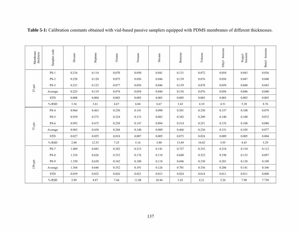
137

Table 5-1: Calibration constants obtained with vial-based passive samplers equipped with PDMS membranes of different thicknesses.

M

embr

ane

thic

knes

s

Sam

pler

cod

e

Hex

ane

Hep

tane

Oct

ane

Non

ane

Dec

ane

Ben

zene

Tolu

ene

Ethy

l- b

enze

ne

Prop

yl-

benz

ene

But

yl-

benz

ene

25 μ

m

PS-1 0.216 0.114 0.070 0.050 0.041 0.131 0.072 0.054 0.043 0.036

PS-2 0.228 0.120 0.075 0.056 0.046 0.139 0.076 0.056 0.047 0.040

PS-3 0.231 0.123 0.077 0.056 0.046 0.139 0.078 0.059 0.048 0.043

Average 0.225 0.119 0.074 0.054 0.044 0.136 0.076 0.056 0.046 0.040

STD 0.008 0.004 0.003 0.003 0.003 0.005 0.003 0.003 0.002 0.003

% RSD 3.36 3.61 4.67 6.04 6.67 3.43 4.10 4.51 5.28 8.76

75 μ

m

PS-4 0.964 0.463 0.250 0.141 0.090 0.501 0.250 0.157 0.108 0.079

PS-5 0.939 0.375 0.224 0.133 0.083 0.382 0.209 0.140 0.100 0.072

PS-6 0.993 0.475 0.258 0.147 0.094 0.514 0.251 0.155 0.108 0.080

Average 0.965 0.438 0.244 0.140 0.089 0.466 0.236 0.151 0.105 0.077

STD 0.027 0.055 0.018 0.007 0.005 0.073 0.024 0.009 0.005 0.004

% RSD 2.80 12.53 7.25 5.16 5.80 15.69 10.02 5.95 4.43 5.29

150 μm

PS-7 1.409 0.683 0.382 0.215 0.141 0.727 0.352 0.218 0.154 0.112

PS-8 1.334 0.626 0.332 0.176 0.118 0.680 0.325 0.198 0.133 0.097

PS-9 1.350 0.630 0.342 0.180 0.118 0.696 0.330 0.201 0.138 0.109

Average 1.364 0.646 0.352 0.191 0.126 0.701 0.336 0.206 0.141 0.106

STD 0.039 0.032 0.026 0.021 0.013 0.024 0.014 0.011 0.011 0.008

% RSD 2.89 4.87 7.44 11.08 10.44 3.43 4.21 5.26 7.90 7.750

138

After observing the results from the experiments, the thicknesses of the membrane material

(cut from the same sheet of membrane as that used for this study) were measured using an

optical microscope. Overall, the thickness was found to deviate by as much as ± 75% from

the manufacturer’s specification (75 µm) at different locations on a one square foot sheet of

the membrane. When measured at different locations of a specific 1 square inch piece of the

membrane, the thicknesses were within 100 ± 20 µm. The pieces of membranes required for

the samplers were cut from a small area which would have avoided large variations in the

thickness. The results of this experiment indicated the importance of proper control of the

membrane thickness. It was not practically possible to determine the variations in the

thickness within the small area of 21.4 mm2 used for each and every passive sampler. To

avoid any problems due to such variations, the membranes cut with the cutting tool were

weighed, and the weights were used as a control for the membrane thickness used for the

exposure experiments for all subsequent exposure studies.

As discussed in Chapter 3, there was a good correlation of ln(k) plot against LTPRI when the

k was measured with the 75 µm thick membranes. The same correlation was then tested for k

determined with different thicknesses of the membrane. The plots for the n-alkanes are

shown in Figure 5-1 for the three membrane thicknesses. A slight deviation from a straight

line correlation was observed for all three membrane thicknesses with the curvature being

more pronounced for the 25 µm thick membranes (correlation coefficient of 0.9552). This

can be attributed to the starvation effect, which affects the net uptake rates of the various

analytes differently depending on the permeability of PDMS towards these analytes. The ln

(k) vs LTPRI correlations with 75 μm and 150 μm membranes were generally good,

suggesting that they were equally good choices for vial-based passive samplers. It should

however be possible to use the 25 µm membrane when the air flow velocity around the

sampler is expected to be high (to reduce the starvation effect), in which case lower

quantification limits and lower residence times (as discussed in Chapter 2, Section 2.1.2)

could be obtained. Further, shorter deployment time would be required when compared to 75

or 150 µm thick membranes to obtain the same quantification limits.

139

Figure 5-1: ln(k) vs. LTPRI correlations for n-alkanes and for various membrane thicknesses

Similarly to the observation for the n-alkanes, a larger deviation from straight line correlation

was observed for aromatic compounds with the 25 µm thickness membrane when compared

to 75 and 150 µm thick membranes (Figure 5-2). This reiterated the significance of the

starvation effect observed for the 25 µm thick membranes.

Figure 5-2: ln(k) vs. LTPRI correlations for aromatic compounds and for various membrane

thicknesses

R² = 0.9787

R² = 0.9289

R² = 0.9704

-3.60

-3.10

-2.60

-2.10

-1.60

-1.10

-0.60

-0.10

0.40500 600 700 800 900 1000 1100 1200

ln(k

)

LTPRI

ln(k) vs. LTPRI correlation - aromatic compounds

▲ 150 μm

♦ 75 μm

■ 25 μm

R² = 0.9895

R² = 0.9552

R² = 0.9909

-3.70-3.20-2.70-2.20-1.70-1.20-0.70-0.200.300.80

400 500 600 700 800 900 1000 1100

ln(k

)

LTPRI

ln(k) vs. LTPRI correlation

▲ 150 μm ♦ 75 μm ■ 25 μm

140

5.2.2 Effect of membrane area

The calculated area of the membrane exposed to air for the 1.8 mL vial was 21.4 mm2, and

that for the 0.8 mL vial was 11.5 mm2. Accordingly, the calibration constants for any analyte

determined using the 0.8 mL vial should be higher by ~1.9 times than those determined using

the 1.8 mL vial. The calibration constants determined using the two types of vials and their

ratios for each analyte are provided in Table 5-2. The ratios of the calibration constants

ranged from 3.05 for n-hexane to 2.20 for butyl benzene, and there was a clear decreasing

trend with an increase in LTPRI.

The observed results could be attributed to several factors. The most important factor is that

the opening in the aluminum cap, which should define the area of exposure for the sampler,

is slightly smaller than the inner diameter of the glass vial (Figure 3-5, Chapter 3).

Consequently, there is a possibility for the air to penetrate between the membrane and the

aluminum cap. Analyte transport into these tiny crevices will occur by molecular diffusion

and hence the effect will be less pronounced for compounds with lower diffusion

coefficients.

141

Table 5-2: Calibration constants and their reproducibilities for n-alkanes and aromatic hydrocarbons determined with 1.8 mL and 0.8

mL vials.

k

n-he

xane

Ben

zene

n-he

ptan

e

Tolu

ene

n-oc

tane

Ethy

l ben

zene

n-no

nane

o-xy

lene

Prop

yl b

enze

ne

n-de

cane

But

yl b

enze

ne

1.8 mL vials

Average (n=3) 0.671 0.384 0.337 0.189 0.170 0.117 0.102 0.100 0.082 0.074 0.063

STDev 0.115 0.053 0.050 0.026 0.019 0.014 0.009 0.010 0.007 0.006 0.005

%RSD 17.058 13.904 14.852 13.701 11.062 11.829 8.905 10.248 8.660 8.345 8.633

0.8 mL vials.

Average (n=4) 2.048 1.055 0.916 0.498 0.431 0.292 0.242 0.245 0.191 0.167 0.138

STDev 0.102 0.073 0.082 0.046 0.045 0.030 0.027 0.026 0.020 0.019 0.016

%RSD 4.960 6.878 8.932 9.200 10.322 10.163 11.153 10.776 10.225 11.519 11.490

Ratio of average k 0.8 /k1.8

3.05 2.75 2.72 2.64 2.53 2.49 2.37 2.45 2.32 2.24 2.20

142

Another factor which could result in disproportionate changes in the uptake rates is perhaps

due to analyte transfer mechanism from the inner surface of the membrane to the sorbent.

The concentration “on” the membrane surface, on the sorbent side, is required to be zero for

the sampler to work properly. However, this might not necessarily be the case. The diameter

of the membrane area exposed to the sample for the 0.8 mL vial was 3.8 mm. The packing of

the sorbent within this area was visually examined and it was found that the first layer of the

sorbent particles did not cover the entire area of the membrane uniformly, as illustrated in

Figure 5-3. This uneven packing could be attributed to the adhesive nature of the membrane

and could affect the uptake rate ratios disproportionately for different analytes. This is due to

the different diffusion coefficient of the analytes within the interstitial space between the

membrane and the first layer of sorbent particles.

Figure 5-3: The monolayer of sorbent particles in contact with the PDMS membrane of the

sampler.

A plot of ln(k) vs. LTPRI however showed similar correlation as observed before, as

illustrated in Figure 5-4. This indicates that the correlations are still valid when the vial size

is 0.8 mL as opposed to the 1.8 mL vial used in this project.

143

Figure 5-4: ln(k) vs. LTPRI correlation determined for n-alkanes with 1.8 mL and 0.8 mL

vials.

5.2.3 Effect of exposure duration

The calibration constants of n-hexane determined by exposing the TWA-PDMS samplers for

durations ranging from 1 to 9 days are shown in Table 5-3. The calibration constant could not

be determined for exposures shorter than 24 hours because the amount of the analyte

collected by the sampler was too small at the concentration selected for quantification. Data

presented in Table 5-3 are remarkably consistent, proving that exposure duration did not have

a significant effect on the uptake rates up to 9 days. This observation is critical for TWA

concentration determination as it allows for the sampler to be deployed for long time periods

without compromising the quality of the data. Consequently, the limits of detection and

quantification for the analytes can be reduced.

y = -0.0056x + 2.8473R² = 0.9803

y = -0.0063x + 4.3941R² = 0.9807

-3.0

-2.5

-2.0

-1.5

-1.0

-0.5

0.0

0.5

1.0300 500 700 900 1100

ln(k

)

LTPRI

ln(k) vs. LTPRI

2mL vials - alkanes

0.8mL vials - alkanes

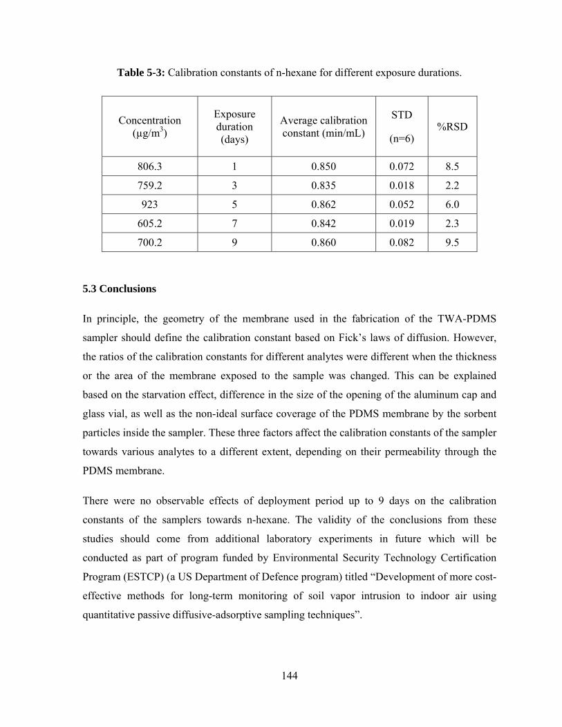
144

Table 5-3: Calibration constants of n-hexane for different exposure durations.

Concentration (µg/m3)

Exposure duration (days)

Average calibration constant (min/mL)

STD

(n=6) %RSD

806.3 1 0.850 0.072 8.5

759.2 3 0.835 0.018 2.2

923 5 0.862 0.052 6.0

605.2 7 0.842 0.019 2.3

700.2 9 0.860 0.082 9.5

5.3 Conclusions

In principle, the geometry of the membrane used in the fabrication of the TWA-PDMS

sampler should define the calibration constant based on Fick’s laws of diffusion. However,

the ratios of the calibration constants for different analytes were different when the thickness

or the area of the membrane exposed to the sample was changed. This can be explained

based on the starvation effect, difference in the size of the opening of the aluminum cap and

glass vial, as well as the non-ideal surface coverage of the PDMS membrane by the sorbent

particles inside the sampler. These three factors affect the calibration constants of the sampler

towards various analytes to a different extent, depending on their permeability through the

PDMS membrane.

There were no observable effects of deployment period up to 9 days on the calibration

constants of the samplers towards n-hexane. The validity of the conclusions from these

studies should come from additional laboratory experiments in future which will be

conducted as part of program funded by Environmental Security Technology Certification

Program (ESTCP) (a US Department of Defence program) titled “Development of more cost-

effective methods for long-term monitoring of soil vapor intrusion to indoor air using

quantitative passive diffusive-adsorptive sampling techniques”.

145

CHAPTER 6

Indoor and outdoor air sampling at various field locations

Indoor and outdoor air sampling was performed at several locations in North America,

Europe and Asia using both the TWA-PDMS samplers and conventional methods. A

representative selection of the methods and analytical results will be provided in this Chapter.

All field sampling described in this Chapter was performed by Geosyntec Consultants, Inc.,

of Guelph, Ontario. All samplers were fabricated and analyzed at the University of Waterloo.

The comparison between the TWA-PDMS samplers and conventional methods was a “blind”

comparison, because no prior information on the background of the field site and/or analyte

concentrations was available to the University of Waterloo due to client confidentiality

agreements between Geosyntec Consultants and the site owners, and no information from the

conventional samples was available to the University of Waterloo until all the results from

the TWA-PDMS samplers were generated.

The objective of this chapter is to provide a comparison of the results obtained from TWA-

PDMS passive samplers with commercially available samplers. The sampling projects that

will be presented in this chapter are as follows:

• Indoor air sampling with SUMMA™ canisters and TWA-PDMS samplers,

• Indoor and outdoor air sampling with 3M™ OVM 3500 sampler and TWA-PDMS

sampler,

• Sampling from vent pipes and high purge volume (HPV) flow cells using TWA-

PDMS and SUMMA™ canisters and

• Indoor air sampling with TWA-PDMS sampler and SUMMA™ canisters or TAGA

unit.

6.1 Field sampling and analysis methods Passive sampler calibration, fabrication and analysis were performed at the University of

Waterloo. The method described in Chapter 3 was used for the fabrication of the sampler.

Each sampler was transferred to a separate 20 mL scintillation vial and sealed with a

146

threaded, plastic, foil-lined cap and PTFE tape. The scintillation vial was then placed inside a

self-sealing polyethylene bag, as shown in Figure 6-1, followed by shipping the sampler to

the specified location. The samplers were removed from the scintillation vials and installed in

the field either by hanging them from a flexible thread attached to the PTFE loop, or by

fixing a rigid stainless steel wire attached to the mouth of the sampler as shown in Figure 6-2.

A laboratory blank was retained in the laboratory, and one or more trip blanks were included

with each shipment to test for any positive biases in the analytical results. After sampling, the

samplers were repacked in the same scintillation vials, sealed again with the caps and PTFE

tape and shipped back to the University of Waterloo for analysis.

The analytes were different for each of the projects discussed in this Chapter and are listed in

the respective sections. The calibration constants used in the calculation of the concentrations

of the analytes are listed in Table 3-12. The calibration constant of PCE (0.187 min/mL) was

estimated using the ln(k/MW) vs. LTPRI correlation because the experimentally determined

value was not available.

Figure 6-1: Photograph of a TWA-

PDMS sampler packed and shipped to

the field.

Figure 6-2: Photograph showing

supports for sampler installation.

147

6.1.1 Indoor air sampling with SUMMA™ canisters and TWA-PDMS samplers

Sampling with SUMMA™ canisters followed by analysis using US-EPA method TO-15 is

one of the most common methods for VOC sampling and analysis in air, therefore it was

chosen as a benchmark for comparison purposes. An example of a SUMMA™ canister is

shown in Figure 6-3,224 and a photograph of the SUMMA™ Canister and TWA-PDMS

samplers deployed concurrently in the field is shown in Figure 6-4.

TWA-PDMS samplers were deployed in a crawl space inside a dwelling to monitor selected

chlorinated organic compounds (1,1,1-TCA, chloroform, cis-DCE, PCE, trans-DCE and

TCE). Seven passive samplers were deployed for approximately one week (exact exposure

periods are shown in Table 6-1) at four different locations in the crawl space. Analyte

concentrations were monitored concurrently by SUMMA™ canister method over the same

exposure period as that for TWA-PDMS samplers at each of the four locations. The time-

weighted average concentration obtained using the SUMMA™ canisters over a period of 7

days was then used for comparison with the concentration determined using the TWA-PDMS

samplers. All the analyses of SUMMA™ canisters were performed by a commercial

laboratory, while all the TWA-PDMS samplers were analyzed at the University of Waterloo.

The TWA-PDMS samplers were analyzed as described in Chapter 3 except that

chromatographic separation and quantification were performed using the method detailed in

Table 6-2.

148

Table 6-1: Deployment duration of TWA-PDMS samplers and the IDs of SUMMA™

canisters deployed concurrently.

Location Geosyntec SUMMA™ Canister ID

TWA-PDMS sampler code

Deployment Date/Time

Retrieval Date/Time

Total time

(mins)

A SUMMA 1 GS-009 6/1/07 10:56 AM 6/8/07 9:22 AM 9986

B SUMMA 2

GS-005 6/1/07 10:56 AM 6/8/07 9:22 AM 9986

GS-007 6/1/07 10:56 AM 6/8/07 9:22 AM 9986

C SUMMA 3

GS-004 6/1/07 10:40 AM 6/8/07 9:53 AM 10033

GS-006 6/1/07 10:40 AM 6/8/07 9:53 AM 10033

D SUMMA 4

GS-008 6/1/07 9:20 AM 6/8/07 8:56 AM 10056

GS-010 6/1/07 9:20 AM 6/8/07 8:56 AM 10056

Figure 6-3: SUMMA™ canisters

with flow controllers.224

Figure 6-4: SUMMA™ canister and

TWA-PDMS samplers deployed for

comparison purpose.

149

Table 6-2: Gas chromatographic method used for the separation and quantification of

chlorinated compounds.

Gas chromatograph Agilent Technologies, 6890 GC

Detector Electron Capture Detector at 350˚C

Injection mode Split, 275˚C Split ratio 1:10

Injection volume 1 μL Carrier gas Helium at 1.2 mL/min

Oven temperature program 35˚C, 7˚C/min to 220˚C, held for 2 min


Capillary column RTX-5 (95% methyl and 5% phenyl), 30 m x 0.25 mm, 0.25 μm film thickness

Calibration method External standard multipoint calibration


PDMS samplers

TWA-PDMS samplers were deployed in a building to test for the presence of chlorinated

VOCs (same set as listed in Section 6.1.1). Commercially available diffusive-type passive

samplers, 3M™ OVM 3500, were also deployed concurrently to compare the results

obtained from the two samplers. The design of the 3M™ OVM 3500 sampler is described in

detail in Section 1.5.2. One week prior to the concurrent deployment of both types of

samplers, several 3M™ OVM 3500 samplers were deployed for 24 hours. The results of this

measurement will be used in this thesis to show the temporal variability of the concentrations

in the field. All analyses of the 3M™ OVM 3500 samplers were performed by a commercial

laboratory, while the TWA-PDMS samplers were analyzed at the University of Waterloo.

The sampling locations of the TWA-PDMS samplers are listed in Table 6-3. Quantification

150

of the analytes in the samplers was performed using the GC-MS method detailed in Table 6-

4.

Table 6-3: TWA-PDMS sampler codes and the locations at which they were deployed.

Sampler code Location

PS-652 2nd floor of office, inside building

PS-653 1st floor or office, lobby area, inside building

PS-654 1st floor of office, training room, inside building

PS-655 1st floor of office, shop area, inside building

PS-656 Behind office building, outside building

PS-657 main door of office, outside building Table 6-4: GC-MS method used for the separation and quantification of chlorinated

compounds.

Gas chromatograph-Mass spectrometer Instrument Agilent Technologies, 6890 GC - 5973 MS


Split ratio 1:10



Oven temperature program 35˚C for 5 mins, 5˚C/min to 120˚C (held for 0 mins), 30˚C/min to 350˚C (held for 3 minutes)


Capillary column Rxi-1 Ms (100% methylsiloxane), 60 m x 0.32 mm, 1.0 μm film thickness

Quantitation mode Selected Ion Monitoring (three ions for each target analyte as listed in Table 7-3 in the next chapter)

Calibration method External standard, multipoint calibration

151

6.1.3 Sampling from vent pipes and high purge volume (HPV) flow cells using TWA-

PDMS samplers and SUMMA™ canisters

Vent pipes are used in many buildings to connect the sub-slab (below the floor) space to the

atmosphere. Their main function is to minimize vapor intrusion into the building through the

floor of the house, which is achieved by providing a path for the contaminated vapors to be

released into the atmosphere. TWA-PDMS samplers and SUMMA™ canisters were used to

monitor vapor concentrations inside such vent-pipes of a passive (wind-driven) sub-slab

venting system in New Jersey. A photograph of one of the vent pipes is shown in Figure 6-5.

In this project, the samples were collected by deploying the TWA PDMS samplers inside the

vent pipe and just above ground level when there was upward air flow in the pipes. The flow

in the vent pipe was expected to reduce any starvation effect. The TWA-PDMS samples and

the SUMMA™ canisters samples were both taken over a period of 24 hours for TWA

concentration determination.

Figure 6-5: Passive vent pipe

HPV testing, pioneered by Geosyntec Consultants, involves withdrawing sub-slab soil gas at

a steady rate and monitoring the pollutant concentration in the vapor phase over a period of

152

time. In the HPV testing method, samplers are deployed or sampled from a flow-through cell

in the effluent path. At a site in Mexico, the sub-slab soil gas sampling was performed using

TWA-PDMS sampler and SUMMA™ canisters. TWA-PDMS samplers were deployed in the

flow cell for half an hour to an hour, and SUMMA™ canister samples were collected over a

period of 5 minutes during the period the TWA-PDMS sampler was deployed. Because of

the substantial air flow through the flow cell, the starvation effect was expected to be

minimal.

The TWA-PDMS samplers were analyzed using the GC-MS method listed in Table 6-4. The

target analytes were c-DCE, TCE, and PCE for both of the above two sampling projects, and

the TWA-PDMS samplers were analyzed using GC-MS method shown in Table-6-4.

6.1.4 Indoor air sampling with TWA-PDMS sampler and SUMMA™ canisters or

TAGA unit

Indoor air sampling was performed at two buildings at a former military arsenal in New

Jersey to quantify PCE concentrations. These buildings were decommissioned and

redeveloped for commercial use prompting the requirement of pollution monitoring. A

number of TWA-PDMS samplers were deployed for a 2-week period, and the analyte

concentrations obtained from them were compared to those obtained a week earlier from US

EPA TAGA mobile laboratory that makes real-time pollutant concentration measurements.

The principle of operation of TAGA is briefly described in Section 1.1.1.

Figure 6-6: US EPA TAGA mobile laboratory

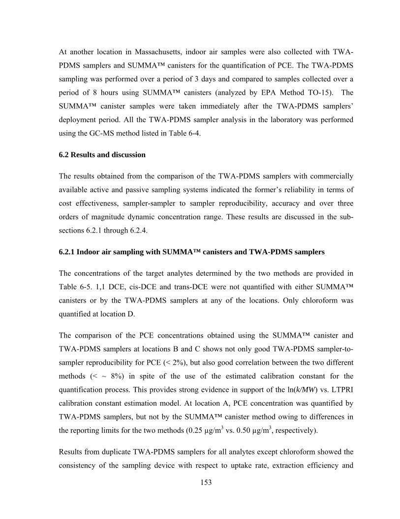
153

At another location in Massachusetts, indoor air samples were also collected with TWA-

PDMS samplers and SUMMA™ canisters for the quantification of PCE. The TWA-PDMS

sampling was performed over a period of 3 days and compared to samples collected over a

period of 8 hours using SUMMA™ canisters (analyzed by EPA Method TO-15). The

SUMMA™ canister samples were taken immediately after the TWA-PDMS samplers’

deployment period. All the TWA-PDMS sampler analysis in the laboratory was performed

using the GC-MS method listed in Table 6-4.


The results obtained from the comparison of the TWA-PDMS samplers with commercially

available active and passive sampling systems indicated the former’s reliability in terms of

cost effectiveness, sampler-sampler to sampler reproducibility, accuracy and over three

orders of magnitude dynamic concentration range. These results are discussed in the sub-

sections 6.2.1 through 6.2.4.

6.2.1 Indoor air sampling with SUMMA™ canisters and TWA-PDMS samplers

The concentrations of the target analytes determined by the two methods are provided in

Table 6-5. 1,1 DCE, cis-DCE and trans-DCE were not quantified with either SUMMA™

canisters or by the TWA-PDMS samplers at any of the locations. Only chloroform was

quantified at location D.

The comparison of the PCE concentrations obtained using the SUMMA™ canister and

TWA-PDMS samplers at locations B and C shows not only good TWA-PDMS sampler-to-

sampler reproducibility for PCE (< 2%), but also good correlation between the two different

methods (< ~ 8%) in spite of the use of the estimated calibration constant for the

quantification process. This provides strong evidence in support of the ln(k/MW) vs. LTPRI

calibration constant estimation model. At location A, PCE concentration was quantified by

TWA-PDMS samplers, but not by the SUMMA™ canister method owing to differences in

the reporting limits for the two methods (0.25 µg/m3 vs. 0.50 µg/m3, respectively).

Results from duplicate TWA-PDMS samplers for all analytes except chloroform showed the

consistency of the sampling device with respect to uptake rate, extraction efficiency and

154

chromatographic quantification methods. At location A, a concentration of 0.83 µg/m3 of

chloroform was quantified by the SUMMA™ canister method but not by the TWA-PDMS

sampler (GS-009 in Table 6-5), even though the quantification limit was 0.21 µg/m3. In

contrast, at location B, a higher concentration was determined using TWA-PDMS sampler

than that obtained with SUMMA™ canisters. This indicated possible short-term chloroform

concentration variations during sampling with the SUMMA™ canisters. However that could

not be confirmed as the sampler to sampler reproducibility for chloroform was good for one

pair of duplicates (~11.5% difference between GS-005 and GS-007) and low for another

(~76.7% difference between GS-004 and GS-006). At location D, the concentration of

chloroform in one of the TWA-duplicates was 0.31 µg/m3 and was < 0.21 µg/m3 for the

other. The reason for this discrepancy with chloroform could not be established.

155

Table 6-5: Comparison of the results from SUMMA™ canisters / TWA-PDMS sampler pairs and comparison of duplicate TWA-

PDMS sampler results. Concentrations are reported in µg/m3. The number followed by “U” indicates that the concentration was below

the reporting limits, and the number itself represents the reporting limit for the specific analyte. Entries with N/A were not analyzed by

the TWA-PDMS sampler.

Location A B C D

SUMMA™

canister

TWA-

PDMS

Sampler

SUMMA™

canister

TWA-PDMS Sampler

Duplicates

SUMMA™

canister

TWA-PDMS Sampler

Duplicates

SUMMA™

canister

TWA-PDMS Sampler

Duplicates

VOCs SUMMA 1 (GS-009) SUMMA 2 (GS-005) (GS-007) SUMMA 3 (GS-004) (GS-006) SUMMA 4 (GS-008) (GS-010)

Sample Start Time: 6/1/07

10:56

6/1/07

10:56

6/1/07

10:56

6/1/07

10:56

6/1/07

10:56

6/1/07

10:40

6/1/07

10:40

6/1/07

10:40

6/1/07

9:20

6/1/07

9:20

6/1/07

9:20

Sample End Time: 6/8/07

9:22

6/8/07

9:22

6/8/07

9:22

6/8/07

9:22

6/8/07

9:22

6/8/07

8:56

6/8/07

8:56

6/8/07

9:53

6/8/07

8:56

6/8/07

8:56

6/8/07

8:56

1,1,1-Trichloroethane 1.2 0.88 1.2 0.98 1.02 1.7 1.36 1.29 0.5 U 0.32 U 0.32 U

1,1-Dichloroethene 0.48 U 2.5 U 0.48 U 2.5 U 2.5 U 0.48 U 2.5 U 2.5 U 0.48 U 2.5 U 2.5 U

Chloroform 0.83 0.21 U 0.81 1.66 1.47 0.73 1.29 0.3 0.49 U 0.21 U 0.31

cis-1,2-Dichloroethene 0.52 U 1.04 U 0.52 U 1.04 U 1.04 U 0.52 U 1.04 U 1.04 U 0.52 U 1.04 U 1.04 U

Tetrachloroethene 0.5 U 0.46 0.5 U 0.52 0.52 0.54 0.58 0.57 0.5 U 0.25 U 0.25 U

trans-1,2-Dichloroethene 0.52 U N/A 0.52 U N/A N/A 0.52 U N/A N/A 0.52 U N/A N/A

Trichloroethene 8.2 5.84 8.1 6.69 6.88 12 8.45 8.17 0.5 U 0.12 U 0.12 U

156


PDMS samplers

The concentrations of all analytes obtained from 3M™ OVM 3500 samplers and TWA-

PDMS samplers are shown in Tables 6-6 and 6-7. In each of the 6 locations shown in these

tables, the first column shows the concentrations of the analytes determined using the 3M™

OVM 3500 samplers deployed at least 5 months before the rest of the sampling and analysis

to give an indication of the temporal variability of the concentrations of different analytes.

Most of the analytes in the sample matrix which were not detected or quantified with the

3M™ OVM 3500 samplers were also not detected or quantified by the TWA-PDMS

samplers. 1,1-DCA and 1,1-DCE were not detected using either of the two samplers. At one

of the locations, trans-1,2-DCE was quantified by the TWA-PDMS samplers, but not by the

3M™ OVM 3500 sampler. In the absence of a reference method for comparison, this could

be perceived as either a false positive result from TWA-PDMS sampler, or a false negative

result from the 3M™ OVM 3500.

The results obtained from both TWA-PDMS and 3M™ OVM 3500 samplers indicated that

the contaminants at the specific locations were mostly TCE and PCE, and little or no

breakdown products (1,1-DCE, trans-1,2-DCE and cis-1,2-DCE) of these two compounds

were present. The higher analyte uptake rates of the 3M™ OVM 3500 (and hence a lower

reporting limit) samplers enabled TCE to be detected at all locations. When using the TWA-

PDMS sampler, however, TCE was detected only at location 2. This should not be perceived

as a disadvantage of the TWA-PDMS sampler, as the duration of the exposure can easily be

increased to improve the quantification limits. Also, the quantification limits of the

chromatographic method can be lowered by making large volume injections of the CS2

extract, using thermal desorption instead of solvent extraction, or adjusting the ratio of

solvent to adsorbent. The concentrations of PCE were high enough to be detected by the

TWA-PDMS samplers at all locations. The concentrations of PCE determined by TWA-

PDMS samplers were in all cases slightly lower than those obtained using 3M™ OVM

samplers with the difference ranging from 9.5% to 41.2%. Again, in the absence of a

reference method it is impossible to say whether either of the methods was biased.

157

Table 6-6: Comparison of results between 3M™ OVM 3500 sampler (abbreviated as 3M-OVM) and TWA-PDMS samplers. The

concentrations are reported in µg/m3. The number followed by “U” indicates that the concentration was below reporting limits and the

number itself represents the reporting limit for the specific analyte.

Sample Type: Indoor Air

Sample Location: Location 1 Location 2 Location 3 Location 4

Sample I.D.: PS-03 PDM-03 PS-653 PS-04 PS-04D PDM-04 PS-654 PS-05 PDM-05 PS-655 PS-06 PDM-01 PDM-02 PS-652

Sampler Type 3M-OVM

3M-OVM

TWA-PDMS

3M-OVM

3M-OVM

3M-OVM

TWA-PDMS

3M-OVM

3M-OVM

TWA-PDMS 3M-OVM 3M-OVM 3M-

OVM TWA-PDMS

Sample Start Time: 9/21/08 15:23

2/27/09 17:13

2/27/09 17:16

9/21/08 15:28

9/21/08 15:29

2/27/09 17:23

2/27/09 17:25

9/21/08 15:30

2/27/09 17:33

2/27/09 17:35

9/21/08 15:40

2/27/09 16:55

2/27/09 17:03

2/27/09 17:00

Sample End Time: 9/22/08 15:25

3/6/09 11:25

3/6/09 11:23

9/22/08 15:28

9/22/08 15:30

3/6/09 11:53

3/6/09 11:57

9/22/08 15:33

3/6/09 11:36

3/6/09 11:39

9/22/08 15:41

3/6/09 11:09

3/6/09 11:14

3/6/09 11:17

1,1-Dichloroethane 0.2 U 0.1 U 2.0 U 0.2 U 0.2 U 0.1 U 2.0 U 0.2 U 0.1 U 2.0 U 0.2 U 0.1 U 0.1 U 2.0 U

1,1-Dichloroethene 0.2 U 0.1 U 2.6 U 0.2 U 0.2 U 0.1 U 2.6 U 0.2 U 0.1 U 2.6 U 0.2 U 0.1 U 0.1 U 2.6 U

1,2-Dichloroethene (cis) 0.2 U 0.55 1.2 U 0.2 U 0.2 U 0.46 1.2 U 0.2 U 0.81 1.2 U 0.2 U 0.55 0.64 1.2 U

1,2-Dichloroethene (trans) 0.2 U 0.1 U 1.6 U 0.2 U 0.2 U 0.1 U 2.0 0.2 U 0.1 U 1.6 U 0.2 U 0.1 U 0.1 U 1.6 U

1,1,1-Trichloroethane 0.2 U 0.1 U 1.5 U 0.2 U 0.2 U 0.13 1.5 U 0.2 U 0.11 1.5 U 0.2 U 0.12 0.10 1.5 U

Tetrachloroethene (PCE) 1.68 3.27 2.3 1.70 1.60 3.98 3.6 1.76 1.23 0.9 1.62 2.91 3.05 1.9

Trichloroethene (TCE) 1.46 0.22 0.6 U 1.74 1.62 0.26 0.7 1.67 0.24 0.6 U 0.91 0.21 0.25 0.6 U

158

Table 6-7: Comparison of results between 3M™ OVM 3500 sampler (abbreviated as 3M-

OVM) and TWA-PDMS samplers. Concentrations are reported in µg/m3. The number

followed by “U” indicates that the concentration was below reporting limits and the number

itself represents the reporting limit for the specific analyte.

Sample Type: Outdoor Air

Sample Location: Location 5 Location 6

Sample I.D.: PS-01 PDM-07 PS-657 PS-02 PDM-06 PS-656

Sampler Type 3M-OVM 3M-OVM

TWA-PDMS 3M-OVM 3M-OVM TWA-

PDMS

Sample Start Time: 9/21/08 15:15

2/27/09 17:50

2/27/09 17:51

9/21/08 15:18

2/27/09 17:41

2/27/09 17:43

Sample End Time: 9/22/08 15:15

3/6/09 11:28

3/6/09 11:31

9/22/08 15:19

3/6/09 11:46

3/6/09 11:49

1,1-Dichloroethane 0.2 U 0.1 U 2.0 U 0.2 U 0.1 U 2.0 U

1,1-Dichloroethene 0.2 U 0.1 U 2.6 U 0.2 U 0.1 U 2.6 U

1,2-Dichloroethene (cis) 0.2 U 0.97 1.2 U 0.2 U 0.57 1.2 U

1,2-Dichloroethene (trans) 0.2 U 0.1 U 1.6 U 0.2 U 0.1 U 2.5

1,1,1-Trichloroethane 0.2 U 0.24 1.5 U 0.2 U 0.14 1.5 U

Tetrachloroethene (PCE) 0.41 1.87 1.1 0.42 0.98 0.8

Trichloroethene (TCE) 0.58 0.35 0.6 U 0.50 0.22 0.6 U

6.2.3 Vent pipe and HPV test sampling with TWA-PDMS samplers and SUMMA™

canisters

Figure 6-7 shows the correlation plot of the concentrations of PCE determined using the

TWA-PDMS samplers and by either the SUMMA™ canister or TAGA. The experiments

indicated a very strong correlation between the two methods over two to three orders of

magnitude for each analyte and an overall correlation over ~4 orders of magnitude for all the

analytes put together. The correlation indicated two data points (marked as A in the chart) for

which the deviations from the 1:1 correlation line was higher than that for the rest. However,

159

the TCE to PCE ratio in that sample was the same as that observed for other samples taken at

the same location. The correlation also indicated no negative bias in the concentrations

obtained from TWA-PDMS samplers which indicated that there was no starvation effect.

These experiments suggested that TWA-PDMS passive samplers could be an economic

alternative to expensive conventional methods of quantifying pollutant concentration in sub-

slab soil gas.

Figure 6-7: Correlation between the concentrations determined in HPV flow cell and passive

vent-pipe using TWA-PDMS samplers and SUMMA™ canisters. “A” indicates two data

points for which the deviations from the 1:1 correlation were higher than that for the rest.

6.2.4 Indoor air sampling with TWA-PDMS samplers and SUMMA™ canisters or

TAGA unit

Correlation of PCE concentrations obtained from TWA-PDMS samplers, SUMMA™

canisters and TAGA unit are shown in Figure 6-8. Similar to the observation made in section

1

10

100

1,000

10,000

100,000

1 10 100 1000 10000 100000

TWA

-PD

MS

Sam

pler

con

cent

ratio

n (µ

g/m

³)

SUMMA™ canister oncentration (µg/m³)

TWA-PDMS vs. SUMMA™ canisters - HPV and passive vent samples

Passive Vent PCEPassive Vent TCEPassive Vent cDCEHPV Test PCE

A

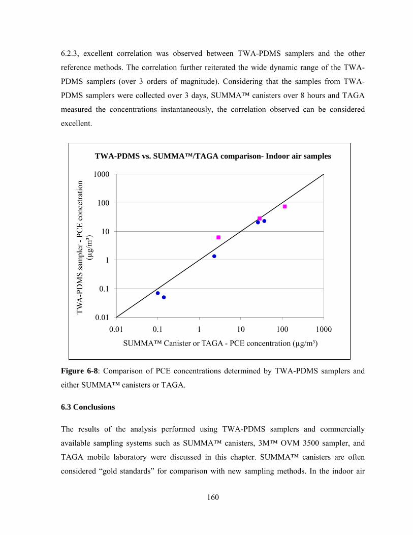
160

6.2.3, excellent correlation was observed between TWA-PDMS samplers and the other

reference methods. The correlation further reiterated the wide dynamic range of the TWA-

PDMS samplers (over 3 orders of magnitude). Considering that the samples from TWA-

PDMS samplers were collected over 3 days, SUMMA™ canisters over 8 hours and TAGA

measured the concentrations instantaneously, the correlation observed can be considered

excellent.

Figure 6-8: Comparison of PCE concentrations determined by TWA-PDMS samplers and

either SUMMA™ canisters or TAGA.

6.3 Conclusions

The results of the analysis performed using TWA-PDMS samplers and commercially

available sampling systems such as SUMMA™ canisters, 3M™ OVM 3500 sampler, and

TAGA mobile laboratory were discussed in this chapter. SUMMA™ canisters are often

considered “gold standards” for comparison with new sampling methods. In the indoor air

0.01

0.1

1

10

100

1000

0.01 0.1 1 10 100 1000

TWA

-PD

MS

sam

pler

-PC

E co

ncet

ratio

n (µ

g/m

³)

SUMMA™ Canister or TAGA - PCE concentration (µg/m³)

TWA-PDMS vs. SUMMA™/TAGA comparison- Indoor air samples

161

sampling experiments, excellent correlations were observed between the concentrations

determined using SUMMA™ canisters and the TWA-PDMS samplers for all analytes but

chloroform. Furthermore, comparison of the concentrations obtained from SUMMA™

canisters and TAGA with TWA-PDMS samplers indicated good correlation between the two

methods and an overall linearity of 6 orders of magnitude for the TWA-PDMS samplers.

3M™ OVM 3500 sampler is a commercially available passive sampler for the analysis of

volatile organic compounds in air. The results obtained from the two methods generally

showed comparable concentrations. Analyte uptake rates for TWA-PDMS samplers were

lower than those for the 3M™ OVM samplers, hence the latter could quantify TCE at lower

concentration levels than the former.

The HPV testing method pioneered by Geosyntec Consultants in combination with the use of

TWA-PDMS samplers proved to be a useful tool in monitoring temporal variability of

analyte concentration without any bias related to starvation effects. TWA-PDMS sampling in

wind driven passive vents using TWA-PDMS samplers also showed very good correlations

with the results obtained with SUMMA™ canisters and indicated no starvation effect. The

results obtained from TAGA compared well with those obtained from TWA-PDMS

samplers.

In all the comparisons, PCE concentrations determined using TWA-PDMS samplers were

estimated from the ln(k/MW) vs. LTPRI correlation rather than determined experimentally,

yet they still showed good correlations with the values obtained using the reference methods,

which is another indication that the calibration constant estimation model works well.

162

CHAPTER 7

Soil gas sampling and analysis

Soil gas surveys are important for determining the presence, composition, source and

distribution of contaminants in soil. The application of TWA-PDMS samplers for such

purposes was tested at several locations and a representative selection of the methods and

analytical results will be presented in this thesis. All field sampling projects described in this

chapter were performed either by Geosyntec Consultants, Inc. of Guelph, ON, or Tauw

Scientific Inc., Belgium, for their clients at various locations in Europe and in North

America. Soil gas sampling application described here included samples collected at various

depths and distances from buildings under evaluation for potential vapor intrusion (exterior

samples), as well as samples collected at shallow depths beneath floor slabs (interior

samples). The consultants’ goal was to characterize or monitor the nature and extent of

subsurface VOC vapors. Our research goal at the University of Waterloo was to demonstrate

the applicability and advantages of the TWA-PDMS sampling technology for such

contaminant mapping purposes by comparing it with existing technologies whenever

possible along with prior knowledge of the contaminant history at the selected locations.

Soil gas sampling is often challenging because of high soil moisture content, variable

permeability, different drilling methods and inter-operator variability. With respect to soil

gas sampling using TWA-PDMS samplers, the aspects discussed in section 4.5.5, related to

the effect of the linear flow velocity of air on the sampling rate are critical to understand and

properly interpret the soil gas concentrations determined. This will be dealt with under the

discussion sections for each of the sampling programs described in this chapter.

7.1 Field sampling and analysis methods

Passive sampler calibration, fabrication and analysis were performed at the University of

Waterloo. The method described in Chapter 3 was used for the fabrication of the sampler.

The method described in Chapter 6 was used for the packing and shipping of the samplers to

and from the laboratory. The holding time between sampling and analysis was generally less

than 30 days, and the samples were refrigerated during storage.

163

In this section, sampling performed at three different locations will be described:

• Sub-slab vapor sampling using TWA-PDMS samplers and SUMMA™ canisters at

Knoxville, TN,

• Soil gas sampling in Belgium using TWA-PDMS samplers and GORE™ modules,

and

• Sub-slab vapor sampling at a location in Italy using TWA-PDMS samplers.

The first method involved comparison with standard methods, the second involved

comparison with a commercially available diffusive-type sampler, and the third was an

application in soil gas concentration mapping.

7.1.1 Sub-slab vapor sampling using TWA-PDMS samplers and SUMMA™ canisters

Sub-slab vapor samples were collected with TWA-PDMS samplers and SUMMA™ canisters

at a location in Knoxville, TN. SUMMA™ canister samples were collected one week prior to

the deployment of the TWA-PDMS samplers from 0.5 inch holes drilled into the floor. The

vapour samples were collected for a period ranging between 5 and 10 minutes at 200 mL/min

using the flow controller in the SUMMA™ canister. The TWA-PDMS samplers were

introduced into holes of 0.75 inch diameter (of varying depths depending on the thickness of

the concrete). The samplers were hung from a rigid metal wire in such a way as to be

approximately an inch from the bottom of the hole, and the hole was sealed with a temporary

seal made of rubber wrapped with aluminum foil sufficient to prevent air-flow into or out of

the drilled hole. The major target analytes at the site were TCE and PCE. All sample

processing was performed using GC-ECD as shown in Table 6-2 earlier.

7.1.2 Soil gas sampling in Belgium with TWA-PDMS samplers and GORE™ modules

In this study, soil gas sampling was performed at a contaminated site using 438 TWA-PDMS

samplers deployed at a regular spacing of about 30 m throughout the site. The area of the test

site was approximately 1000 m long and 600 m wide. The contaminants possibly present at

the site included chlorinated ethanes, ethenes and benzenes, BTEX, PAHs and PCBs. The

contaminants originated from different industries located in the area. Head-to-head

comparison was made between the results obtained from TWA-PDMS samplers and the

164

commercially available GORE™ modules at 80 locations (see Chapter 1 for the description

of the GORE™ module). The GORE™ modules were installed, retrieved and analyzed

independently by their manufacturer.

The list of the target analytes, determined based on the history of the manufacturing facilities

and their activities in the region, is shown in Table 7-1. The analytes marked with asterisks

are those for which the calibration constants were estimated based on the correlation of the

calibration constant with the linear temperature programmed retention index of the analytes.

Table 7-1 also indicates the minimum concentration (reporting limits) that could be

quantified using the TWA-PDMS samplers calculated based on the calibration constant, one

week deployment period and quantification limits of the chromatographic methods. The low

calibration constants (or high uptake rates) for PAHs indicate that very high linear flow

velocity of air across the surface of the sampler is required for sampling without starvation

effect.

165

Table 7-1: Target analytes, their calibration constants and reporting limits for a one week

exposure of the TWA-PDMS sampler used for soil gas sampling in Belgium. “*” indicates

analytes for which estimated calibration constants were used for quantitfication purposes.

Analyte Calibration constant (min/mL)

Reporting limit for 1 week exposure period in µg/m3

1,1-Dichloroethylene 1.223 2.48

t-Dichloroethylene 0.755 1.55

1,1-Dichloroethane 0.964 1.86

c-Dichlroethylene 0.524 1.12

Chloroform 0.514 1.08

1,2-Dichloroethane 0.388 0.80

1,1,1-Trichloroethane 0.787 1.54

Benzene 0.466 0.85

Carbontetrachloride 0.667 1.35

Trichloroethylene 0.305 0.56

1,1,2-Trichloroethane* 0.255 0.55

Toluene 0.236 0.48

Perchloroethylene* 0.187 0.43

Chlorobezenze* 0.276 0.69

1,1,1,2-Tetrachloroethane* 0.166 0.29

Ethylbenzene 0.151 0.29

p,m-Xylene 0.146 0.30

1,1,2,2-Tetrachloroethane* 0.112 0.26

o-Xylene 0.131 0.31

1,3-Dichlorobenzene* 0.134 0.38



Naphthalene* 0.039 0.039

Acenaphthylene* 0.009 0.009

Acenaphthene* 0.009 0.009

Fluorene* 0.008 0.008

Phenanthrene* 0.003 0.003

Anthracene* 0.002 0.002

Fluoranthene* 0.002 0.002

Pyrene* 0.0008 0.001

166

7.1.2.1 Sampler deployment methods A 2 inch diameter borehole was drilled to a depth of 1.2 meters using a core barrel shown in

Figure 7-1. The TWA-PDMS samplers were then suspended inside the borehole at a depth of

1 m from the ground surface. The water table depth in that area was around 4 m. Once the

sampler was in place, the borehole was sealed with a simple technique illustrated in Figure 7-

2. A rigid metal rod was first inserted into a black plastic bag and an aluminum foil was

wrapped snugly enough to hold during insertion and removal, but loosely enough to expand

out against the walls of the borehole after insertion (Figure 7-2 (A) and (B)). The assembly

was then pushed into the borehole to a depth of approximately 0.7 m from the surface (Figure

7-2 (C) and (D)) which allowed vapor sampling for the TWA-PDMS samplers from a 0.5 m

long segment of the borehole. The surface of the borehole was then sealed with a wooden

tapered cork.

Figure 7-1: Field personnel coring a hole for the deployment of TWA-PDMS samplers and

GORE™ Modules

167

Figure 7-2: Photographs of (A) – Aluminum foil being wrapped around the plastic cover,

(B) – crunching the aluminum foil for snug fit, (C) – the assembly being inserted into the

borehole and (D) – the completed borehole sealing process.

GORE™ modules were deployed into separate boreholes at a lateral distance of 0.3 m from

the selected boreholes where the TWA-PDMS samplers were deployed. The GORE™

A

DC

B

168

module (the white part in Figure 7-3) was inserted into the borehole and secured using a

thread on the outside such that the module rested at approximately the same distance from

the ground surface as that of the TWA-PDMS samplers in their respective boreholes. The

boreholes were then sealed at the surface with wooden corks. The surface appearance of the

ground after the boreholes were sealed is shown in Figure 7-4. It has to be noted that the

effective vapor space in the borehole from where TWA-PDMS sampling was performed was

0.5 m of the borehole, while it was the entire 1.2 m for the GORE™ modules (proprietary

specification). On the other hand, the sealing method used for the TWA-PDMS samplers was

much more effective, and the risk of soil gas dilution with atmospheric air in the borehole

was much smaller than with the GORE™ modules.

Figure 7-5 shows locations of the 438 TWA-PDMS samplers. The lateral spacing between

the samplers was different at different locations, but was generally kept at 30 m whenever

possible. Figure 7-6 shows the locations of the 80 GORE™ modules installed for head-to-

head comparison purposes.

Figure 7-3: Deployment of the

GORE™ module inside a

borehole.

Figure 7-4: Ground surface appearance after

the deployment of the TWA-PDMS samplers

and the GORE™ modules.

GORE™ module

TWA-PDMS sampler

GORE™ module

169

Figure 7-5: Borehole locations for the TWA-PDMS sampler’s deployment

170

Figure 7-6: Borehole locations where the TWA-PDMS samplers and GORE™ modules

were deployed within 30 cm of each other. Red spots indicate GORE™ modules, and green

spots indicate TWA-PDMS samplers.

7.1.2.2 TWA-PDMS sampler solvent desorption and chromatographic methods

The extraction scheme shown in Figure 7-7 was used for the quantification of the target

analytes trapped in the TWA-PDMS samplers. The target analytes included PAHs, which are

extracted from Anasorb 747® with poor efficiency using CS2. The extraction method was

therefore modified by including a second extraction with

171

Figure 7-7: Schematic of the solvent desorption and subsequent chromatographic analysis peformed for the quantification of the

various groups of target analytes.

Transfer sorbent and

PDMS membrane from

the sampler to a 4 mL

vial

Analyze 200 µL of the

extract by GC MS

Add 1 mL CS2 and

extract for 30 mins

with intermittent

shaking

Analyze 200 µL of the

extract by GC FID/ECD

Use FID data for

TPH analysis

Use ECD data for

detecting the PCBs

Add 500 µL of toluene to the extract after

step 1 and step 2. Sonicate for 20 mins

and transfer extract to new crimp-top vial

Analyze by

GC-MS

Quantify 8 target

compounds (PAHs)

Quantify 22 target analytes including

chlorinated ethenes, ethanes and benzenes,

as well as BTEX

Step 1

Step 2

172

toluene combined with sonication for the extraction and analysis of the PAHs. The respective

recovery rates for the PAHs were determined based on this extraction method and applied

while estimating the concentrations in the sample as described in more detail in the

paragraphs below.

The sorbent in the sampler along with the PDMS membrane were transferred to 4 mL vials

and extracted with 1 mL aliquots of freshly distilled CS2 for 30 minutes with intermittent

shaking. 0.4 mL of the extract was transferred to two GC crimp cap vials with 200 µL inserts

in each of them, and then crimped to seal. The content of the first vial was analyzed by GC-

MS for all analytes except the PAHs and PCBs using the method listed in Table 7-2. GC-MS

was operated in the SIM mode and the ions used for the quantification of each analytes are

listed in Table 7-3.

Table 7-2: GC-MS method used for the separation and quantification of BTEX and

chlorinated compounds.

GC-MS Instrument Agilent Technologies, 6890 GC - 5973 MS


Split ratio 1:10





Capillary column Rxi-1 MS (100% methylsiloxane), 60 m x 0.32 mm, 1.0 μm film thickness

Quantification mode Selected Ion Monitoring (three ions for each analyte, except where noted, as in Table 7-3)


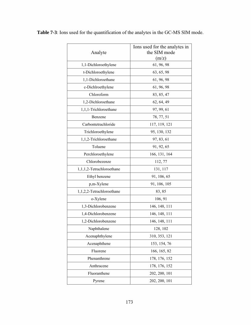
173

Table 7-3: Ions used for the quantification of the analytes in the GC-MS SIM mode.

Analyte Ions used for the analytes in

the SIM mode (m/z)

1,1-Dichloroethylene 61, 96, 98

t-Dichloroethylene 63, 65, 98

1,1-Dichloroethane 61, 96, 98

c-Dichlroethylene 61, 96, 98

Chloroform 83, 85, 47

1,2-Dichloroethane 62, 64, 49

1,1,1-Trichloroethane 97, 99, 61

Benzene 78, 77, 51

Carbontetrachloride 117, 119, 121

Trichloroethylene 95, 130, 132

1,1,2-Trichloroethane 97, 83, 61

Toluene 91, 92, 65

Perchloroethylene 166, 131, 164

Chlorobezenze 112, 77

1,1,1,2-Tetrachloroethane 131, 117

Ethyl benzene 91, 106, 65

p,m-Xylene 91, 106, 105

1,1,2,2-Tetrachloroethane 83, 85

o-Xylene 106, 91

1,3-Dichlorobenzene 146, 148, 111



Naphthalene 128, 102

Acenaphthylene 310, 353, 121

Acenaphthene 153, 154, 76

Fluorene 166, 165, 82

Phenanthrene 178, 176, 152

Anthracene 178, 176, 152

Fluoranthene 202, 200, 101

Pyrene 202, 200, 101

174

The second vial was used for the determination of the Total Petroleum Hydrocarbon (TPH)

concentration and screening for PCBs in the sample. The determination of TPH requires a

GC with an FID (sensitive to most organic compounds), while the detection of PCBs requires

a GC with an ECD (sensitive to chlorinated compounds). To achieve this, the eluent from the

GC capillary column was split into two using a Graphpack® “Y” splitter, and the eluent was

analyzed by both FID and ECD. The GC method listed in Table 7-4 was used for this

purpose. Total petroleum hydrocarbons were then estimated based on the procedure

described in Chapter 3.

Table 7-4: GC method used for the separation and quantification of total petroleum

hydrocarbons and for the detection of PCBs.

GC Instrument Agilent Technologies, 6890 GC


Split ratio 1:10





Capillary column VF-1 Ms (100% methylsiloxane), 15 m x 0.25 mm, 0.5 μm film thickness

Detector / calibration method for TPH estimation

Flame Ionization detector / external standard, multipoint calibration with benzene

Detector / calibration method for the detection of PCB’s Electron Capture Detector / no calibration performed.

No theoretical and/or experimental work was performed to determine the uptake rates of the

PCBs by the TWA-PDMS samplers, as quantitative analysis was not required by the

customer. Consequently, only a visual comparison of the peak pattern in the chromatograms

obtained using the ECD for the samples with a chromatogram obtained by injecting a 1 µL

sample solution containing 1 µg/mL of Aroclor 1254 (a mixture of PCB congeners) was

175

carried out to screen for the presence or absence of PCBs. The extraction efficiency of the

PCB congeners in Aroclor 1254 was examined by spiking 10 µL of a 100 µg/mL solution in

a 4 mL vial containing 250 mg of Anasorb 747®, and following the same procedure of

extraction and sample injection as described earlier for PCB analysis.

A 0.5 mL aliquot of toluene was then added to the same 4 mL vial (from which 400 µL

aliquot of the CS2 extract was already removed) described in the above paragraphs, and

further extracted with sonication for 20 minutes at room temperature. The toluene-CS2

extract was centrifuged, and the supernatant was transferred to another vial containing a 100

µL insert and analyzed by GC-MS for the semi-quantification of PAHs. The GC-MS method

(operated in the SIM mode) used for the analysis is listed in Table 7-5.

Table 7-5: GC-MS method used for the separation and quantification of PAHs in the

extracted solvent.

GC-MS Instrument Agilent Technologies, 6890 GC – 5975B MS


Split ratio 1:10





Capillary column VF-5 MS (95% methylsiloxane , 5% Phenyl), 30 m x 0.25 mm, 1.0 μm film thickness

Quantification mode Selected Ion Monitoring (three ions for each analyte, except where noted, as in Table 7-3)


Recovery rates for all target analytes were determined by spiking standard solutions of the

analytes onto the Anasorb 747® and a cut PDMS membrane (same dimension as that used in

the samplers) in a 4 mL vial. The vials were capped after spiking and were allowed to

equilibrate for 2 days for one set of 6 vials and 2 weeks for a a second set of 6 vials at room

temperature before extraction with CS2 and chromatographic analysis. This was done to

176

investigate any difference in recovery rates due to holding time of the sampler between its

retrieval in the field and extraction/analysis in the laboratory. The target analytes were

divided into four groups, and the recovery rates were determined for these groups separately

in the maner explained above. Recovery rates obtained from the two-week storage period

were applied when calculating analyte concentrations in the soil gas so as to correct for the

time required for sampler transportation from Belgium to Waterloo, ON.

7.1.3 Sub-slab soil gas sampling in Italy with TWA-PDMS samplers

Sub-slab soil gas sampling was performed to determine the concentrations of chlorinated

ethanes and ethenes at various locations in a manufacturing facility with known history of

using various chlorinated solvents. A total of 37 PDMS samplers were deployed for sub-slab

vapor sampling. A total of 6 target VOCs were analyzed: PCE, TCE, cis-DCE, vinyl

chloride, 1,1-DCE and chloroform. The calibration constants of all the target analytes except

vinyl chloride are listed in Table 7-1. An estimated calibration constant of 2.08 min/mL

(based on ln(k/MW) vs. LTPRI correlation as described in Chapter 3) was used for the latter.

An electric hammer drill was first used to drill a one inch diameter hole in the floor as shown

in Figure 7-8. A one foot temporary steel casing was used as a guide to insert the sampler to

the desired depth into the drilled hole. The casing was then removed and the top of the hole

was sealed to prevent air exchange across the slab during the deployment period. After five

days of sampler exposure, the samplers were retrieved and shipped to the University of

Waterloo for sample analysis. Both the deployment and the retrieval of the 37 samplers took

only several hours, thereby reducing the field cost drastically compared to conventional soil

gas sampling using SUMMA™ canisters which would have taken two to three days for the

same number of samples. The samples received at the University of Waterloo were analyzed

using the GC-MS method parameters listed in Table 7-2. Analyte extraction was performed

using the sample extraction scheme presented in Figure 3-16. All analyses were performed

within one week from the time the samples were retrieved from the field.

Figur

the T

7.2 R

The r

advan

appli

7.2.1

The c

Figur

by th

meth

the s

appro

of ma

samp

re 7-8: Phot

TWA-PDMS

Results and d

results from

ntages and p

cations. The

Sub-slab va

concentratio

re 7-9 indica

he TWA-PD

od. This wa

stagnant air

oximately on

agnitude for

plers at all t

tographs of (

sampler at a

discussion

the projects

performance

ey are presen

apor sampl

ons obtained

ated a negati

DMS sample

as a direct co

matrix aro

ne order of m

r all but one

the location

(A) – a hole

a predetermi

s described

e of the TW

nted in the fo

ing using T

from the tw

ive bias in th

ers compare

onsequence o

ound the sam

magnitude fo

sampler. If

s, a nearly

177

being drille

ined depth in

above provi

WA-PDMS sa

ollowing thre

WA-PDMS

wo sampling

he concentra

d to those o

of the starva

mpler. This

or most of th

the starvatio

constant ne

ed into the fl

n the hole.

ided extensiv

ampler when

ee sub-sectio

S samplers a

g systems at

ations of bot

obtained usi

ation effect,

s effect resu

he samplers,

on effects w

egative bias

loor and (B)

ve informati

n used for s

ons.

and SUMMA

different lo

th TCE and

ing the SUM

which is un

ulted in a n

and was les

were to be ide

should hav

– deployme

ion regardin

soil gas sam

A™ caniste

cations show

PCE determ

MMA™ can

navoidable d

negative bia

s than two o

entical for a

ve been obse

ent of

ng the

mpling

ers

wn in

mined

nister

due to

as of

orders

all the

erved

178

(assuming that there were no temporal variations during the time the concentrations were

determined by the two methods). The variation in negative bias indicated that the starvation

effect was different for different samplers, which could be explained based on the different

depths of the core holes, as well as the differences in soil matrix permeability towards TCE

and PCE. There was however a positive correlation between the two methods sufficient for

routine use of the TWA-PDMS sampler for such application in determining the relative

concentrations of various pollutants at different locations. It should also be noted that the

starvation effect is unavoidable for not just the sampler discussed here, but for any other

passive sampler in general.

Figure 7-9: Comparison of PCE and TCE concentrations obtained from TWA-PDMS

samplers and SUMMA™ canisters. The solid straight line represents a 1:1 correlation, and

the dotted lines represent one and two orders of magnitude difference correlations.

The results of this project indicated the importance of the starvation effect as applied for soil

gas sampling using the TWA-PDMS samplers. One potential method to reduce such

starvation effect is to increase the depth and width of the core hole in which the sampler is

0.1

1

10

100

1000

10000

100000

1000000

10000000

0.1 1 10 100 1000 10000 100000 1000000 10000000Con

cent

ratio

n fr

om T

WA

-PD

MS

Sam

pler

(µg/

m3 )

Concentration from SUMMA™ canister (µg/m3)

SUMMA™ canister and TWA-PDMS sampler results

TCE

PCE

179

deployed. In that way, the inside surface area of the core hole can be increased, and

consequently more analyte can diffuse into the core hole in unit time to compensate for its

removal from the vapour phase due to uptake into the sampler. As a result, the core hole

diameter was increased to 2 inches in the project which is discussed next.

7.2.2 Soil gas sampling in Belgium

Out of the 438 samplers deployed in the field, only 405 were retrieved and analyzed, as some

of the samplers could not be retrieved due to the borehole collapsing onto them. A detailed

analytical report on the concentrations of various target analytes at various locations is

available in Excel spreadsheet format on the accompanying compact disc. The electronic

version of the Excel sheet in pdf format is also available (Appendix A). The significant

observations are discussed in this section.

Figure 7-10 shows a typical chromatogram of a standard solution of a mixture of chlorinated

compounds and BTEX obtained using the GC-MS method outlined in Table 7-2.

Chlorobenzene and 1,1,1,2-tetrachloroethane peaks co-eluted at 17.4 minutes, therefore their

unique fragment ions, 112 and 131, respectively, were used for quantification. The same was

true for 1,1,2,2-tetrachloroethane and o-xylene. In this case, the unique fragment ions m/z 83

and 91, respectively, were used for the quantification. Figure 7-11 shows a typical

chromatogram of a sample solution obtained using the GC-MS method outlined in Table 7-2.

Figure 7-12 shows chromatograms obtained from the injection of the standard solution of 1

µg/mL of Aroclor 1254 in CS2 and an equivalent concentration after extraction of the spiked

Aroclor 1254 with 1 mL CS2. These two chromatograms were used for comparison with the

sample extracts to visually identify the presence/absence of PCBs in soil gas.

The extraction efficiencies of all the analytes (Table 7-6) except PAHs and dichlorobenzenes

were greater than 84%, with relative standard deviations of less than 5.3% (n=6) for both 48

hours and 2 weeks holding period. The extraction efficiencies varied between 48% and 78%

for the PAHs and dichlorobenzenes, with a relative standard deviations ranging between

3.2% and 12.3% (n=6). The low extraction efficiencies for PAHs and dichlorobenzenes were

expected, as Anasorb 747® is known to be unsuitable for PAHs and SVOCs in general.

180

While a total of 405 TWA-PDMS samplers were analyzed, only 80 GORE™ modules were

installed for comparison purposes. Accordingly, contaminant profiles determined on the

basis of PDMS sampler results indicated more contaminated locations than the GORE™

modules. The major contaminants determined using both types of samplers were chlorinated

compounds like TCE and PCE, as well as benzene and traces of naphthalene. No PCBs were

detected using either of the two methods. This was consistent with the knowledge of the

history of the location. Contamination profiles determined by TWA-PDMS samplers and

GORE™ modules for these analytes were generally similar and indicated the same

concentration hot spots.

181

Figure 7-10: A typical chromatogram of a standard solution of chlorinated compounds and BTEX obtained using GC-MS method outlined in Table 7-2: (1) 1,1-DCE (2) t-DCE

(3) 1,1-DCA (4) c-DCE (5) CF (6) 1,2-DCA (7) 1,1,1-TCA (8) benzene (9) CT (10) TCE (11) 1,1,2-TCA (12) toluene (13) PCE (14) chlorobenzene (15) 1,1,1,2-TetCA (16) ethyl

benzene (17) p,m-Xylene (18) 1,1,2,2-TetCA (19) o-xylene (20) 1,3-DCB (21) 1,4-DCB (22) 1,2-DCB (23) naphthalene.

1 2 3

4

8

5 6 7

9

10 11

12

13

14,15

21

16 17

18,19

22

20

23

182

Figure 7-11: A typical chromatogram obtained from a sample solution using the GC-MS method outlined in Table 7-2: (8) benzene

(12) toluene (16) ethyl benzene (17) p,m-xylene (19) o-xylene.

8 12

16

17

19

183

Figure 7-12: Chromatograms obtained by the injection of 1 µL of Aroclor 1254 in CS2: (A) 1 µg/mL standard solution of Aroclor

1254 and (B) 1 µg Aroclor 1254 spiked onto to Anasorb 747® and PDMS membrane and extracted with 1 mL CS2.

A B

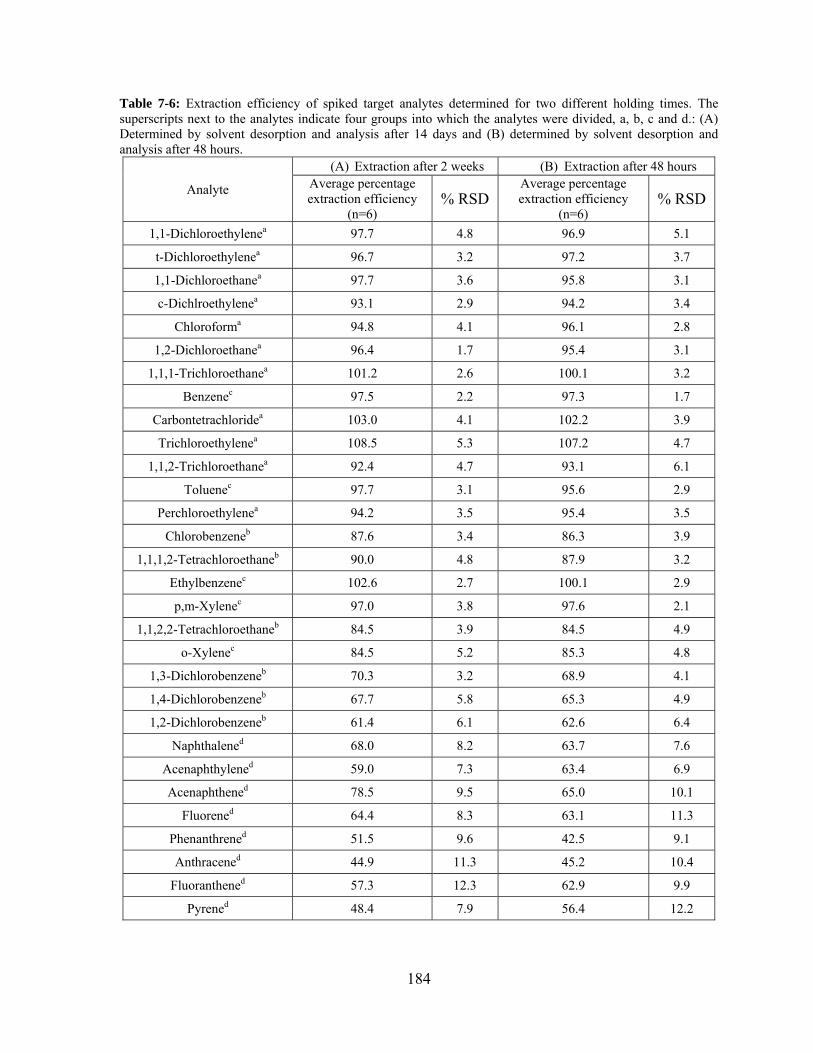
184

Table 7-6: Extraction efficiency of spiked target analytes determined for two different holding times. The superscripts next to the analytes indicate four groups into which the analytes were divided, a, b, c and d.: (A) Determined by solvent desorption and analysis after 14 days and (B) determined by solvent desorption and analysis after 48 hours.

Analyte

(A) Extraction after 2 weeks (B) Extraction after 48 hours Average percentage extraction efficiency

(n=6) % RSD

Average percentage extraction efficiency

(n=6) % RSD

1,1-Dichloroethylenea 97.7 4.8 96.9 5.1

t-Dichloroethylenea 96.7 3.2 97.2 3.7

1,1-Dichloroethanea 97.7 3.6 95.8 3.1

c-Dichlroethylenea 93.1 2.9 94.2 3.4

Chloroforma 94.8 4.1 96.1 2.8

1,2-Dichloroethanea 96.4 1.7 95.4 3.1

1,1,1-Trichloroethanea 101.2 2.6 100.1 3.2

Benzenec 97.5 2.2 97.3 1.7

Carbontetrachloridea 103.0 4.1 102.2 3.9

Trichloroethylenea 108.5 5.3 107.2 4.7

1,1,2-Trichloroethanea 92.4 4.7 93.1 6.1

Toluenec 97.7 3.1 95.6 2.9

Perchloroethylenea 94.2 3.5 95.4 3.5

Chlorobenzeneb 87.6 3.4 86.3 3.9

1,1,1,2-Tetrachloroethaneb 90.0 4.8 87.9 3.2

Ethylbenzenec 102.6 2.7 100.1 2.9

p,m-Xylenec 97.0 3.8 97.6 2.1

1,1,2,2-Tetrachloroethaneb 84.5 3.9 84.5 4.9

o-Xylenec 84.5 5.2 85.3 4.8

1,3-Dichlorobenzeneb 70.3 3.2 68.9 4.1



Naphthalened 68.0 8.2 63.7 7.6

Acenaphthylened 59.0 7.3 63.4 6.9

Acenaphthened 78.5 9.5 65.0 10.1

Fluorened 64.4 8.3 63.1 11.3

Phenanthrened 51.5 9.6 42.5 9.1

Anthracened 44.9 11.3 45.2 10.4

Fluoranthened 57.3 12.3 62.9 9.9

Pyrened 48.4 7.9 56.4 12.2

185

In the case of sampling and analysis with TWA-PDMS samplers, the soil gas sampling,

analysis and calculations to convert the mass sorbed by the sampler into concentration in the

gas phase were carried out in the same fashion as for air sampling discussed earlier. The

calibration constants used in the calculations were determined (or estimated based on ln(k)

vs. LTPRI correlation) under the conditions of optimum flow of air across the surface of the

sampler. Since there was no air circulation in the sealed boreholes, the final concentration

determined was most likely lower than the true concentration because of the starvation effect.

Further, since the starvation effect increases with increasing uptake rates, the magnitude of

the negative bias in principle should also be higher when moving down from 1,1-DCE to

pyrene in Table 7-6. The magnitude of this starvation effect was discussed in Section 7.2.1.

However, as the borehole dimensions and the depth at which the samplers were deployed

were similar in all cases, the method still should have provided accurate relative

concentrations provided that the permeability of the soil matrix at different locations was

similar. In the case of GORE™ modules, a proprietary method for the calculation of the soil

gas concentrations was used by the manufacturer.

The plot of benzene concentrations determined by the TWA-PDMS samplers vs. the

corresponding concentrations determined by the GORE™ modules at different locations is

shown in Figure 7-13. The plot revealed that the concentrations reported by the GORE™

modules were mostly lower than those determined using the TWA-PDMS samplers. None of

the data points in the correlation plot approached the 1:1 line above 100 µg/m3 as measured

by the TWA-PDMS sampler, which indicated that GORE™ modules were not effectively

estimating high benzene concentrations. This was in agreement with the findings of a project

conducted by the US EPA Environmental Technology Certification Program on the use of

GORE™ modules, which noted that pollutant concentrations were not effectively determined

at high concentrations.113

186

Figure 7-13: Correlation plot for benzene concentrations determined at different locations

using the TWA-PDMS samplers and the GORE™ modules. The straight line represents a 1:1

correlation.

As noted in Section 1.7.1, the uptake rate of the GORE™ module is substantially higher

because of its geometry, as well as the diffusive properties of the GoreTex® material used as

the barrier. For example, the uptake rate of toluene is ~ 13 mL/min for the GORE™ modules

as opposed to 4.2 mL/min for the TWA-PDMS samplers.225 The GoreTex® material prevents

liquid water from being transported across it. However, it still lets water vapor to pass

through (with the sampler having a higher uptake rate for water vapor than for the rest of the

target analytes), which could have very likely led to premature sorbent saturation in the

GORE™ modules. The exposure to humid environment and to high analyte concentrations

can easily saturate the sorbent resulting in the correlation plot similar to that observed for

benzene. The PDMS membrane used as a barrier in the TWA-PDMS samplers on the other

hand has low permeability towards water compared to other analytes (and hence lower

uptake rate), which allows the sorbent and the sampler to function properly at higher

concentrations and/or for longer deployment times. The potential bias of TWA-PDMS

sampler results is mainly related to the starvation effect, whereas the results from the

GORE™ modules might be biased due to the starvation effect, sorbent saturation and lack of

0.1

1

10

100

1000

0.1 1 10 100 1000

GO

RE™

mod

ule

(µg/

m3 )

TWA-PDMS Sampler (µg/m3)

Benzene

187

a proper theoretical model for converting the amounts found in the samplers into analyte

concentrations in the soil gas. Consequently, it can be concluded that the results from the

TWA-PDMS samplers should be closer to true values than those from the GORE™ modules.

Figures 7-14 and 7-15 show the concentration contour plots of benzene determined using the

TWA-PDMS samplers and the GORE™ modules, respectively. Comparing the two figures,

the concentration maps identify some of the same areas of elevated concentrations (it should

however be pointed out that the color scales in two contour maps are different by more than

an order of magnitude, reflecting the negative bias of the GORE™ modules as indicated in

Figure 7-13). For example, it can be noticed that locations A and B in Figure 7-14 show

concentration profiles similar to locations A1 and B1 in Figure 7-15. There were also

locations where benzene was detected by the TWA-PDMS samplers, but not by the GORE™

modules. This was partly due to the fact that a larger number of TWA-PDMS samplers were

used to generate the profiles compared to the number of GORE™ modules.

Figure 7-14: Benzene concentration profile determined using the TWA-PDMS samplers. A

and B are locations in the field that can be compared with locations A1 and B1 in Figure 7-

15.

B

A

188

Figure 7-15: Benzene concentration profile determined using the GORE™ modules. A1 and

B1 are locations in the field that can be compared with locations A and B in Figure 7-14.

The correlation plot of the corresponding BTEX concentrations obtained by the two types of

samplers (shown in Figure 7-16) indicated again a trend similar to that seen for benzene. This

was likely due to the fact that of all the BTEX, only benzene was found in considerable

amounts at various locations by both samplers. Similar to the benzene correlation, none of

the data points in the plot approached the 1:1 line above 100 µg/m3 as determined by the

TWA-PDMS samplers attributable to sorbent saturation and increased starvation effects for

the GORE™ modules. The highest BTEX concentration determined by TWA-PDMS

sampler was ~ 3100 µg/m3, while that determined by GORE™ module was only ~ 69 µg/m3.

The concentration profiles of total BTEX determined by the two samplers are shown in

Figures 7-18 and 7-19. Visually, the similarities in the concentration profiles were not

entirely obvious because of the 1-2 order of magnitude difference in the color scale.

B1

A1

189

Figure 7-16: Correlation plot for BTEX concentrations determined at different locations

using the TWA-PDMS samplers and the GORE™ modules. The straight line represents a 1:1

correlation.

Figure 7-17: BTEX concentration profile determined using the TWA-PDMS samplers

0.1

1

10

100

1000

10000

0.1 1 10 100 1000 10000

GO

RE™

mod

ule

(µg/

m3 )


BTEX

190

Figure 7-18: BTEX concentration profile determined using the GORE™ modules

Figure 7-19 shows that naphthalene concentrations reported by the GORE™ modules were

generally 1-3 orders of magnitude higher than those reported using TWA-PDMS samplers,

which is in contrast to the trend with benzene and BTEX concentrations (as well as TCE and

PCE profiles which will be discussed later). A possible reason for this observation could be

the increased starvation effect experienced by the TWA-PDMS samplers, which becomes

worse with increasing air – PDMS partition coefficient. The estimated uptake rate of

naphthalene is ~ 25.6 mL/min for TWA-PDMS samplers, which should be greater than that

for the GORE™ modules (since uptake rate is ~ 13 mL/min for toluene by GORE™ modules

as per ref. 2, it should be much lower than that for naphthalene owing to the lower diffusion

coefficient of naphthalene in air). Further, the TWA-PDMS sampler has not been tested in

the laboratory for its applicability to the determination of semi-volatile organic compounds.

As the partition coefficient of the analyte increases to a level like that for naphthalene, a

potential problem could be that PDMS itself becomes a good sink, hence the analyte might

not be as efficiently transferred to the sorbent in the sampler as with smaller molecules. The

concentration contour plots of naphthalene determined by the two samplers are shown in

Figures 7-20 and 7-21. The elevated concentrations determined at locations C, D and E in

191

Figure 7-20 from TWA-PDMS samplers were similar to those at locations C1, D1 and E1

determined using GORE™ modules as shown in Figure 7-21.

Figure 7-19: Correlation plot for naphthalene concentrations determined at different

locations using the TWA-PDMS samplers and the GORE™ modules. The straight line

represents a 1:1 correlation.

Figure 7-20: Naphthalene concentration profile determined using the TWA-PDMS samplers.

C, D and E are the locations in the field which can be compared with C1, D1 and E1 in

Figure 7-21.

0.01

0.1

1

10

100

1000

10000

0.01 0.1 1 10 100 1000 10000

GO

RE™

mod

ule

(µg/

m3 )


Naphthalene

C

D

E

192

Figure 7-21: Naphthalene concentration profile determined using the GORE™ modules. C1,

D1 and E1 are the locations that can be compared with locations C, D and E in Figure 7-20.

There was a relatively good correlation between the absolute concentrations obtained using

the two samplers for PCE (shown in Figure 7-22) when compared to the other analytes

discussed so far. The correlation plot indicated no saturation effect for PCE determined by

the GORE™ module at concentrations up to ~ 120 µg/m3. As a result of the good correlation,

the concentration contour plots of PCE obtained by the two methods, shown in Figures 7-22

and 7-23, identified similar elevated concentrations levels (locations E and E1 in Figures 7-

23 and 7-24).

C1

D1

E1

193

Figure 7-22: Correlation plot for PCE concentrations determined at different locations using

the TWA-PDMS samplers and the GORE™ modules. The straight line represents a 1:1

correlation.

Figure 7-23: PCE concentration profile determined using the TWA-PDMS samplers. E is the

location that can be compared with the location E1 in Figure 7-24.

0

1

10

100

1000

0.1 1 10 100 1000

GO

RE™

mod

ule

(µg/

m3 )


Tetrachloroethylene

E

194

Figure 7-24: PCE concentration profile determined using the GORE™ modules. E1 is the

location that can be compared with location E in Figure 7-23.

The comparison of absolute concentrations of TCE (Figure 7-25), indicated that the

concentrations obtained from GORE™ modules were generally lower than those obtained

using the TWA-PDMS samplers. This was similar to the trends observed with benzene and

BTEX and can be attributed to starvation and saturation effect for the GORE™ modules.

Furthermore, this is consistent with results presented at the Midwestern States Risk

Assessment Symposium - Soil Gas Demonstration Program in 2006, where the GORE™

modules showed good correlation to active soil gas samples for PCE, but underestimated

TCE concentrations by typically a factor of 7.226 The difference in the concentrations

measured at any location by the two methods was however within one order of magnitude at

most of the locations and within 3 orders of magnitude at all the locations. Nevertheless,

there was still a similarity in the concentration hot spot locations identified in the two contour

plots. (Figures 7-27 and 7-28). Examples are regions F and G in Figure 7-26 corresponding

to the regions F1 and G1 in Figure 7-27.

E1

195

Figure 7-25: Correlation plot for trichloroethylene concentrations determined at different

locations using the TWA-PDMS samplers and the GORE™ modules. The straight line

represents a 1:1 correlation.

Figure 7-26: Trichloroethylene concentration profile determined using the TWA-PDMS

samplers. F and G are locations that can be compared with location F1 and G1 in Figure 7-

27.

0.10

1.00

10.00

100.00

1000.00

0.1 1 10 100 1000

GO

RE™

mod

ule

(µg/

m3 )


Trichloroethylene

G F

196

Figure 7-27: Trichloroethylene concentration profile determined using the GORE™

modules. F1 and G1 are locations that can be compared with locations F and G in Figure 7-

26.

The correlation for TPH concentrations determined using the two samplers was poor, as

shown in Figure 7-28. With two exceptions, all the data points indicated a negative bias in

the concentrations reported by GORE™ modules. In the cases discussed above for benzene,

BTEX, and TCE, the saturation effect for GORE™ module was noticeable above 100 µg/m3

as determined by the TWA-PDMS samplers. The TPH correlation plot shown here is a

further proof for such an effect. The TWA-PDMS samplers were found to have a much

broader dynamic range of 6 orders of magnitude.

G1 F1

197

Figure 7-28: Correlation plot for total petroleum hydrocarbon concentrations determined at

different locations using the TWA-PDMS samplers and the GORE™ modules. The straight

line represents a 1:1 correlation.

Concentration contour plots of total petroleum hydrocarbons (TPH) determined by the two

samplers are shown in Figures 7-29 and 7-30. It was difficult to compare the two profiles

because of the large variation in the color scales for the two profiles due to the large negative

bias in the results reported using the Gore modules. However, there were still concentration

hot-spots which were identified using both samplers. The variation could also have arisen

due to the different quantification methods used to arrive at the final TPH concentration. The

GORE™ modules analysis method used GC-MS for quantification, while TPH quantification

with the TWA-PDMS samplers was based on GC-FID analysis and estimated calibration

constants. The GORE™ method is based on the assumption that all organic compounds have

similar response factors when using a MS as a detector, which is not true. Furthermore, the

uptake rates of most of the compounds detected by GC-MS were unknown. Consequently,

1

10

100

1000

10000

100000

1000000

1 10 100 1000 10000 100000 1000000

GO

RE™

mod

ule

(µg/

m3 )


Total petroleum hydrocarbons

198

the estimate of the TPH concentrations obtained using the GORE™ method, based on a

proprietary model, is subject to unknown errors. In the case of TWA-PDMS sampler, a GC-

FID was used for the quantification of TPH. The method, as described in earlier chapters, is

based on the uniform response of FID towards hydrocarbons. Furthermore, the uptake rate of

each compound in the sample can be easily estimated based on the calibration constant vs.

LTPRI correlation. The results from TWA-PDMS samplers can therefore be considered more

accurate than those from the GORE™ modules.


TWA-PDMS samplers.

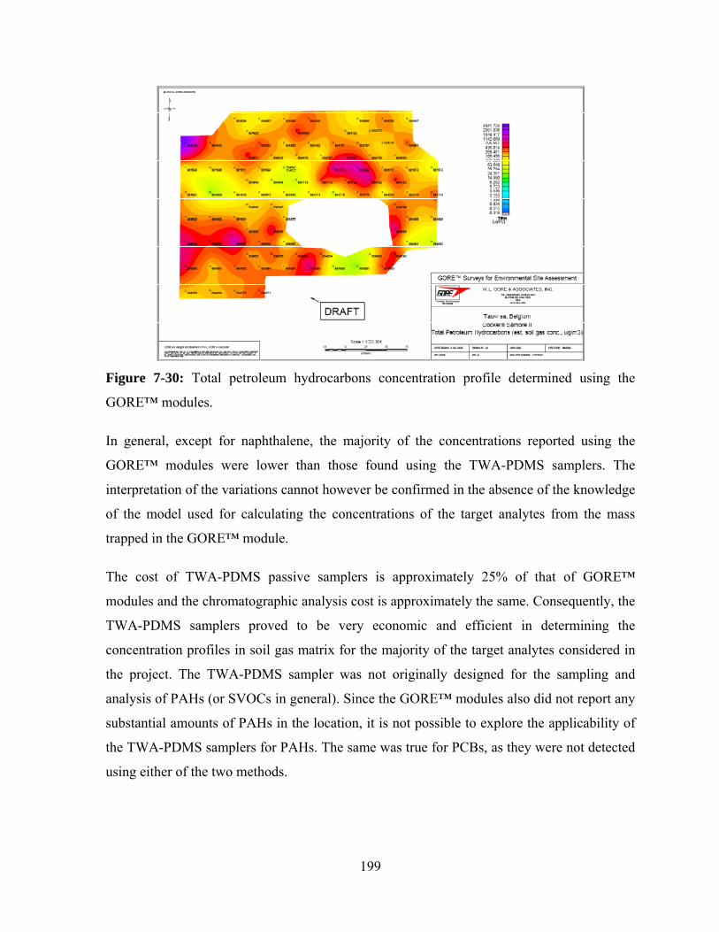
199


GORE™ modules.

In general, except for naphthalene, the majority of the concentrations reported using the

GORE™ modules were lower than those found using the TWA-PDMS samplers. The

interpretation of the variations cannot however be confirmed in the absence of the knowledge

of the model used for calculating the concentrations of the target analytes from the mass

trapped in the GORE™ module.

The cost of TWA-PDMS passive samplers is approximately 25% of that of GORE™

modules and the chromatographic analysis cost is approximately the same. Consequently, the

TWA-PDMS samplers proved to be very economic and efficient in determining the

concentration profiles in soil gas matrix for the majority of the target analytes considered in

the project. The TWA-PDMS sampler was not originally designed for the sampling and

analysis of PAHs (or SVOCs in general). Since the GORE™ modules also did not report any

substantial amounts of PAHs in the location, it is not possible to explore the applicability of

the TWA-PDMS samplers for PAHs. The same was true for PCBs, as they were not detected

using either of the two methods.

200

7.2.3 Sub-slab soil gas sampling in Italy using TWA-PDMS samplers

Analysis of all samplers indicated that vinyl chloride (reporting limit 14.6 µg/m3) and 1,1-

DCE (reporting limit 16.0 µg/m3) were not present in quantifiable amounts in any of the

samples. The concentrations of c-DCE (reporting limit 8.6 µg/m3), chloroform (reporting

limit 1.5 µg/m3), TCE (reporting limit 0.86 µg/m3) and PCE (reporting limit 0.58 µg/m3) are

presented in Table 7-7. The results showed that PCE was the dominant VOC in the soil gas at

the specific site, followed by TCE and traces of c-DCE and chloroform. The elevated

concentrations depicted in Figure 7-31 seemed to be restricted to locations where it was

known that PCE had been used. It was also noticed that the concentration of PCE generally

decreased as the location was further away from the “hot spots” of relatively high

concentrations.

On the basis of the soil gas survey performed during this project, eight locations with the

highest concentrations were selected for drilling, and soil samples were collected for further

analysis for regulatory purposes. The analysis of bulk soil samples had indicated the absence

of any VOCs at the site. This demonstrates that the TWA-PDMS sampler provides

sensitivity that can probe soil samples with much lower concentrations, which is very useful

for assessing the potential health risks via subsurface vapor intrusion to indoor air.

201

Table 7-7: Concentrations of the target analytes determined using the TWA-PDMS samplers

at Lomazzo, Italy.

Sampler code c-DCE (µg/m3) CHCl3 (µg/m3) TCE (µg/m3) PCE (µg/m3)

Apr-03 59.1 2.82 51.7 8.98

Apr-04 11.5 1.62 20.3 12.7

Apr-05 U 1.44 31.1 7.85

Apr-06 9.84 1.85 5 12

Apr-07 21.5 1.97 5.43 12.2

Apr-08 U 1.65 1.53 10.4

Apr-09 U 1.85 2.92 7.07

Apr-10 U 1.62 1.5 25.7

Apr-11 106 2.1 187 6170

Apr-12 22.8 1.54 61.3 1460

Apr-13 8.94 1.75 16.7 536

Apr-14 U 1.49 19.2 450

Apr-15 13.4 1.93 140 10200

Apr-16 13.5 3.55 1610 1550

Apr-17 27.4 1.74 30.2 974

Apr-18 U U 26.5 47

Apr-19 U 2.31 122 16100

Apr-20 U 2.93 133 11800

Apr-21 U 1.7 73.4 4090

Apr-22 U 1.9 62.8 128

Apr-23 U 1.67 8.11 3160

Apr-24 U 2.13 355 13300

Apr-25 116 72.3 4350 729000

Apr-26 U 1.54 26.7 313

Apr-27 U 1.58 1.21 44.8

Apr-28 U U 1.27 1250

Apr-29 U U 21.7 23.3

Apr-30 U U 9.19 33.6

Apr-31 U 2.08 18.1 30.6

Apr-32 U 1.79 100.6 12.7

Apr-33 U 1.8 1.85 9.93

Apr-34 U 1.7 8.03 15.7

Apr-35 U 1.91 18.2 13.6

Apr-36 23.9 3.01 459 108000

Apr-37 23.3 8.55 857 45400

Apr-38 U 1.67 1.92 31.3

Apr-39 U 2.05 9.85 11.4

Apr-40 U 1.58 51.7 2.24

202

Figure 7-31: Concentrations of PCE at various locations determined using TWA-PDMS

samplers. The circled region shows areas of maximum concentration of PCE.

7.3 Conclusions

Soil gas sampling at various indoor as well as outdoor locations was performed using TWA-

PDMS samplers and compared with GORE™ modules and SUMMA™ canisters sampling.

The project at Knoxville, TN, using both the TWA-PDMS samplers and SUMMA™

canisters, showed the importance of the starvation effects in the determination of analyte

concentrations by the TWA-PDMS samplers. The concentrations determined by the TWA-

PDMS samplers showed a general positive correlation, and were within two orders of

magnitude of those determined using SUMMA™ canisters for all the samplers but one.

Soil gas sampling performed at an outdoor location in Belgium alongside commercially

available GORE™ modules showed that concentration profiling can be done with TWA-

PDMS sampler at least as well as with the GORE™ modules, and most likely more

accurately because of the many advantages of the TWA-PDMS samplers in this particular

application. Low permeability of PDMS towards water allowed TWA-PDMS samplers to

203

determine analyte concentrations over a large dynamic range. The major error(s) in

determining the actual concentration from the TWA-PDMS samplers can be attributed only

to the starvation effect, while for the GORE™ modules they can be attributed to the

starvation effect (greater than that for TWA-PDMS samplers for most of the analytes), the

use of a proprietary uptake rate model rather than experimentally determined values, and

sorbent saturation due to high moisture uptake rate. The starvation and saturation effects

together resulted in the GORE™ modules not being able to determine high concentrations

accurately, as opposed to a wide dynamic concentration range for the TWA-PDMS samplers.

Deployment of the TWA-PDMS samplers can be done as easily as with the GORE™

modules at only a fraction of the cost of fabrication. The TWA-PDMS samplers were not

intended for use in sampling of PAHs and need to be further developed in terms of the

sorbent choice and extraction method if this direction is to be pursued further. The GORE™

module on the other hand has been widely used for PAH sampling and analysis.

Sub-slab soil gas sampling and analysis are critical in examining vapor intrusion pathways

and subsequent remediation requirements. TWA-PDMS samplers were demonstrated to be

useful for such an application at Lomazzo, Italy. The concentrations obtained by the TWA-

PDMS samplers were not compared to any accepted method in this project for comparison,

but the general concentration ranges corresponded well to the locations where there was prior

knowledge of the contaminant use. Sub-slab soil gas sampling and analysis is an important

tool to determine pollutant distribution, which is crucial in modeling vapor intrusion

pathways.

204

CHAPTER 8

Summary and future work

8.1 Summary

Passive sampling technology is more advantageous compared to traditional active/grab

sampling techniques due to its low cost, low maintenance requirements, unattended operation

and independence from power sources. In the current project, a new passive sampler was

designed to further improve the potential of the passive sampling technology for routine use

in the field. The merits of the technology have resulted in upcoming commercialization of the

sampler.

One of the fundamental ideas of the project was to design a sampler which would be

inexpensive, allow easy automation of the analytical procedure and reduce the number of

sample preparation steps. The design of the TWA-PDMS sampler developed proved to be

highly economic, and the device can be easily fabricated using supplies available in a

laboratory with little training. Solvent extraction can be carried out within the sampler itself,

followed by introducing the sampler into the GC auto-sampler after changing the aluminum

crimp cap. This method results in reduced potential for contamination, as well as makes the

whole procedure easy for automation.

Calibration constants of 41 model compounds were determined, and a model was developed

to estimate them based on the physicochemical properties of the analytes. The 41 model

analytes included compounds from highly non-polar alkanes to highly polar alcohols. While

it is possible to estimate the calibration constants of diffusive passive samplers by theoretical

calculations using the diffusion coefficients of the analytes in air, it has not been the case

thus far for permeation passive samplers, as the permeability coefficients of the analytes in

the permeation membranes used in the samplers are not easily available. The model

developed within this project based on LTPRI allows for the sampler to be deployed in the

field without prior knowledge of specific analytes in the sample matrix. This is due to the

fact that LTPRIs determined using columns with polydimethylsiloxane stationary phases

depend on partitioning coefficients of the analyte molecules between the carrier gas and the

205

stationary phase, just as the calibration constants of the permeation passive samplers do.

Such a concept of estimation of the calibration constants is very useful not only when the

identity of the analyte is unknown at the time of sampling, but also when determining

summary parameters like total petroleum hydrocarbons in the gas phase using a GC equipped

with a flame ionization detector.

Determining the calibration constants of the 41 model compounds also allowed the

determination of the permeability of polydimethylsiloxane towards various analytes.

Determination of such fundamental properties is an important scientific information for

similar analytical sample preparation/introduction techniques such as PDMS membrane

extraction with a sorbent interface (MESI), PDMS thin film extraction and PDMS membrane

inlet mass spectrometry (MIMS).

An important issue with the performance of passive samplers is the sampling rate variation

when environmental conditions considerably deviate from the laboratory conditions under

which it was determined. Owing to the hydrophobic properties of polydimethylsiloxane, it

was shown that the calibration constants of the sampler towards various analytes are largely

independent on the humidity in the sampling environment. Anasorb 747®, the sorbent used in

the fabrication of the sampler, is characterized by good analyte recovery rates for VOCs

during solvent desorption with carbon disulphide, which positively affects the performance

of the TWA-PDMS sampler.

The calibration constant for a particular analyte is a function of the geometry of the sampler

and the permeability of PDMS towards the analyte. Permeability on the other hand is the

product of the diffusion coefficient of the analyte in PDMS and the partition coefficient of

the analyte between air and the PDMS membrane. With varying temperature, the diffusion

coefficient and the partition coefficient of an analyte vary in opposite directions, which leads

to a partial trade-off in the net permeability. As a result, the dependence of the uptake rate on

temperature is weak. The variations in the calibration constants with temperature were

quantified for various groups of compounds. The variations were in general found to be

slightly larger than those observed with diffusive-type passive samplers. However, with the

knowledge of temperature variations in the field environment, appropriate corrections can

206

always be used based on the energy of activation of permeation values determined in this

project. These values are not only important in understanding the function of the sampler

designed in this project, but also to understand the fundamental transport properties of

PDMS. Such fundamental transport properties in turn can be successfully used for other

PDMS-based analytical techniques, including those mentioned above.

Field sampling and analysis are important parts of validation of any new sampler design. A

number of field sampling events were therefore planned and performed in collaboration with

Geosyntec Consultants and Tauw Scientific Inc. to study the performance of the samplers

under actual field conditions. The analytical results obtained from the TWA-PDMS samplers

were compared to several currently available passive samplers such as SUMMA canisters,

3M™ OVM 3500 samplers, GORE™ modules, and TAGA.

Sampling and analysis by SUMMA™ canisters/EPA method TO-15 are accepted as the

“gold standard” for comparison purposes. Concentrations obtained using TWA-PDMS

samplers indicated excellent correlation with SUMMA™ canister method over 4 orders of

magnitude. Similar excellent results were observed when compared with TAGA mobile

laboratory results also, which, together with the results from SUMMA™ canisters, indicated

an overall dynamic concentration range of the TWA-PDMS samplers of 6 orders of

magnitude. The results from the field sampling and analysis procedures showed that the

TWA-PDMS samplers provided comparable and/or better results when compared to 3M™

OVM 3500 sampler and GORE™ modules. Considering that the cost of the TWA-PDMS

samplers is significantly lower than that of the above mentioned sampling systems, the

overall performance of the sampler can be considered to be very good. The TWA-PDMS

samplers have been shown to work well in indoor air, outdoor air and soil gas matrices.

The project presented in the thesis included theoretical details, determination of the

fundamental calibration data and the effect of geometric and environmental parameters on

the calibration constants. The excellent performance of the sampler observed in the

laboratory resulted in sampling and analysis being performed at more than 20 locations in

North America, Europe, and Asian countries in the past three years alone. The sample

matrices included indoor air, outdoor air, and soil gas. The results from the samplers were

207

used for vapor intrusion studies, soil gas remediation work and screening for pollutants in

dwellings, offices and manufacturing areas. The TWA-PDMS samplers have been shown to

work at least as good as commercially available samplers at a considerably reduced cost and

increased ease of use. The potential for the sampler to be used routinely in the field is

therefore considerable and warrants more detailed studies in many areas which have not been

touched upon in the thesis due to the limited amount of time.

8.2 Future work

The good performance and advantages of the TWA-PDMS sampler resulted in it being

included in a project entitled “Development of more cost-effective methods for long-term

monitoring of soil vapor intrusion to indoor air using quantitative passive diffusive-

adsorptive sampling techniques” and funded by Environmental Security Technology

Certification Program (ESTCP), a US Department of Defence program. The project involves

the comparison of four passive sampling techniques including TWA-PDMS, Radiello®,

Automated Thermal Desorption (ATD®) tube, and SKC Ultra II® samplers. Various aspects

of the different samplers will be considered in this project including a comparison with

industry-accepted standards using statistically designed laboratory and field experiments. The

matrices studied will include indoor air, outdoor air, sub-slab soil gas and soil gas.

The development of the model for the estimation of the calibration constants was based on

the assumption that the diffusion coefficients of the analytes were practically constant, and

that consequently the calibration constants were determined mainly by the partition

coefficients of the analytes between air and the PDMS membrane. While the model worked

well, there are opportunities to further correct for variations in the diffusion coefficients of

the analytes in PDMS membranes. One such method would be to use the concept of inverse

gas chromatographic (IGC) techniques to determine not only the partition coefficients, but

also the diffusion coefficients of the analytes in the membrane. The method of determining

the diffusion coefficients is based on the fact that the chromatographic retention time and the

profile of the eluting peaks are functions of the partition coefficient of the analyte between

the carrier gas and the stationary phase and the diffusion coefficients of the analytes in the

stationary phases and the mobile phase among many other variables. Pawlisch and co-

208

workers determined the diffusion coefficients and solubility parameters for analytes such as

benzene, toluene, and ethylbenzene in polystyrene as early as in 1987.227 Jackson and Huglin

measured diffusion coefficients of chlorobenzene in cross-linked amine-cured epoxy resin.228

Cankurtaran and Yilmaz determined the enthalpy and entropy parameters of selected n-

alkanes in PDMS, a method which could be useful when determining the variations of the

calibration constants of the TWA-PDMS samplers with temperature.229 Zhao and co-workers

demonstrated the applicability of IGC for the determination of the diffusion coefficients of

various n-alkanes in crosslinked PDMS.230

Since determining these parameters using GC can be quicker and easier when compared to

experimentally determining the calibration constants of the analytes in the laboratory, this

method can result in a better model for correlating the calibration constant with retention

parameters in gas chromatography.

An added advantage of developing models based on retention parameters is that the PDMS

membrane can be replaced by various other materials. Such materials can then be

conveniently used as stationary phases in gas chromatographic columns for developing

models for estimating the calibration constants with the changed membrane material.

Alternatively, a custom membrane material can be proposed based on studies of the retention

parameters in columns coated with this material.

The TWA-PDMS sampler developed during this project has been applied mainly for vapour

phase volatile organic compounds sampling and analysis. However, since PDMS is highly

hydrophobic, in principle the sampler should be applicable for sampling volatile organic

compounds from water matrix as well. Demonstrating the applicability of the sampler in

water (and pore water) matrices could in theory provide one sampler for all matrices.

Currently, the analytical extraction method involves solvent desorption with carbon

disulphide. Typically, the carbon disulphide volume used for extraction is 1 mL, and only 1

µL of this extract is injected into the GC for quantifications. Consequently, the quantification

limit for the extraction and analysis is considerably higher than it potentially could be. The

quantification limit can be further reduced either by using large volume injection in GC (with

injection volumes potentially as high as 100 µL), or by switching to a thermally desorbable

209

sorbent. The latter would allow solvent desorption to be replaced with thermal desorption,

which makes it possible to transfer all the analytes collected by the sorbent into the GC

column, thereby greatly reducing the quantification limit of the method. Alternatively,

supercritical fluid extraction of the sorbent can be performed followed by transferring the

analytes completely into the GC using a method similar to the extraction of toluene from

Anasorb 747® demonstrated by Glaser and Shulman.231

The project detailed in this thesis has resulted in a new, highly cost effective permeation-type

passive sampler and has been validated in the laboratory and under field conditions. Many

potential improvements can be made to understand and further develop the technology. The

author firmly believes that the sampler will be well accepted for widespread use in air and

soil gas monitoring applications.

210

Appendix A

Soil gas sampling in Belgium: Analyte concentrations

This appendix is a pdf file containing analyte concentrations determined using TWA-PDMS

samplers at a contaminated site in Belgium.

The file name of this pdf file is “Belgium Project Results – Thesis.pdf”

If you accessed this thesis from a source other than the University of Waterloo, you may not

have access to this file. You may access it by searching for this thesis at

http://uwspace.uwaterloo.ca

211

References

1S. Seethapathy, T. Górecki, X. Li, J. Chromatogr. A 1184 (2008) 234. 2T. Górecki, J. Namieśnik, Trends Anal. Chem. 21 (2002) 276. 3Directive 2004/42/EC of the European Parliament and of the Council on the Limitation of

Emissions of Volatile Organic Compounds Due to the Use of Organic Solvents in

Decorative Paints and Varnishes and Vehicle Refinishing Products and Amending Directive

1999/13/EC, Strasbourg, 2004. 4EPA Compendium Method TO-17, Determination of Volatile Organic Compounds in

Ambient Air Using Active Sampling onto Sorbent tubes, United States Environmental

Protection Agency, Cincinnati, OH, 1999. 5M. Harper, J. Chromatogr. A 885 (2000) 129. 6Hazardous Materials Training Institute, in Site Characterization, Wiley, NJ, 1997. 7K. Badjagbo, S. Sauve, Trends Anal. Chem. 26 (2007) 931. 8M. Liess, M. Leonhardt, Meas. Sci. Technol. 14 (2003) 427. 9Technical note TN-102, http://www.conceptcontrols.com/file/164, accessed on 30th Jul,

2009. 10B.G. Willoughby (Ed.) in Air Monitoring in the Rubber and Plastics Industries, Smithers

Rapra Technology, Billingham, UK, 2003. 11E.D. Palmes, A.F. Gunnison, Am. Ind. Hyg. Assoc. J. 34 (1973) 78. 12P. Mayer, J. Tolls, J.L. M. Hermens, D. Mackay, Environ. Sci. Technol. 37 (2003) 185A. 13J. Pawliszyn, in D. Barceló (Ed.), Comprehensive Analytical Chemistry, Vol. 37,

Elsevier, Amsterdam, 2002, p. 253. 14T.M. Madkour, S.K. Mohamed, A.K. Barakat, Mater. Sci. Technol. 18 (2002) 1235. 15J. Namieśnik, T. Górecki, E. Kozlowski, L. Torres, J. Matheieu, Sci. Total. Environ. 38

(1984) 225. 16J. Comyn (Ed.), Polymer Permeability, Elsevier, England, 1985. 17K.J. Saunders, Int. Environ. Safety, August (1981) 54. 18A. Berlin, R.H. Brown, K.J. Saunders (Eds.), Diffusive Sampling: An Alternative Approach

to Workplace Air Monitoring, CEC Pub. No. 1055EN, Commission of European

Communities, Brussels, 1987.

212

19B.A. Byrne, R.I. Aylott, Concentrator for Removing Organic Materials from Aqueous

Systems, British Patent 1566253, London, UK, 1980. 20A. Södergren, Environ. Sci. Technol. 21 (1987) 855. 21R.H. Brown, M. Curtis, K.J. Saunders, S. Vandendriessche (Eds.), Clean Air at Work -

New Trends in Assessment and Measurement for the 1990s (Proceedings of an

International Symposium Held in Luxenbourg, 9-13 September 1990), Royal Society of

Chemistry, London, 1991. 22J.N. Huckins, J.D. Petty, K. Booij (Eds.), Monitors of Organic Chemicals in the

Environment: Semipermeable Membrane Devices, Springer, NY, 2006. 23R. Greenwood, G. Mills, B. Vrana (Eds.), Passive Sampling Techniques in Environmental

Monitoring, Vol. 48, Elsevier, Amsterdam, 2007. 24W.K. Fowler, Am. Lab. 14 (1982) 80. 25V.E. Rose, J.L. Perkins, Am. Ind. Hyg. Assoc. J. 43 (1982) 605. 26M. Harper, C.J. Purnell, Am. Ind. Hyg. Assoc. J. 48 (1987) 214. 27R.H. Brown, Pure Appl. Chem. 65 (1993) 1859. 28O.J. Levin, R. Lindahl, Analyst 119 (1994) 79. 29B. Kozdron-Zabiegała, J. Namieśnik, A. Przyjazny, Indoor Environ. 4 (1995) 189. 30R.H. Brown, J. Environ. Monit. 2 (2000) 1. 31A. Kot, B. Zabiegała, J. Namieśnik, Trends Anal. Chem. 19 (2000) 446. 32Y. Lu, Z. Wang, J. Huckins, Aquat. Toxicol. 60 (2002) 139. 33R.M. Cox, Environ. Pollut. 126 (2003) 301. 34F. Stuer-Lauridsen, Environ. Pollut. 136 (2005) 503. 35J. Namieśnik, B. Zabiegała, A. Kot-Wasik, M. Partyka, A. Wasik, Anal. Bioanal. Chem.

381 (2005) 279. 36Technology Overview of Passive Sampler Technologies, DSP-4, Interstate Technology and

Regulatory Council (ITRC), Washington, DC, 2006. 37B. Vrana, I.J. Allan, R. Greenwood, G.A. Mills, E. Dominiak, K. Svensson, J. Knutsson, G.

Morrison, Trends Anal. Chem. 24 (2005) 845. 38M. Partyka, B. Zabiegała, J. Namieśnik, A. Przyjazny, Crit. Rev. Anal. Chem. 37 (2007)

51.

213

39G.A. Mills, B. Vrana, I. Allan, D.A. Alvarez, J.N. Huckins, R. Greenwood, Anal. Bioanal.

Chem. 387 (2007) 1153. 40EPA Compendium Method TO-14A, Determination of Volatile Organic Compounds

(VOCs) in Ambient Air Using Specially Prepared Canisters with Subsequent Analysis by

Gas Chromatography, United States Environmental Protection Agency, Cincinnati, OH,

1999. 41EPA Compendium Method TO-15, Determination of Volatile Organic Compounds in Air

Collected in Specially-Prepared Canisters and Analyzed by Gas Chromatography/Mass

Spectrometry, United States Environmental Protection Agency, Cincinnati, OH, 1999. 42www.lancasterlabs.com/environmental/analytical/9050_02.doc, accessed on 31st Jul, 2009. 43A. Rossner, J.P. Farant, J. Occup. Environ. Hyg. 1 (2004) 69. 44S. Heekmann, Non-enantioselective and Enantioselective Determination of Microbial

Volatile Organic Compounds as Tracer for Human Exposure to Mould Growth in

Buildings, Ph.D thesis, University of Basel, Switzerland, 2006. 45N. Yomamoto, T. Matsubasa, S. Mori, K. Suzuki, Anal. Chem. 74 (2002) 484. 46http://products.aerotechpk.com/ProductList.aspx?cid=92912dc1-cdc8-4390-8b8e-

5973583cdd1b&sid=237bcf6a-48e1-448d-8a02-c3b7bbffe1f2, accessed on 23rd Jun, 2009. 47S.A.S. Wercinski and J. Pawliszyn (Eds.), Solid-phase Microextraction - A Practical Guide,

Mercel Dekker, NY, 2009. 48Y. Chen, J. Pawliszyn, Anal. Chem. 75 (2003) 2004. 49M. Vogel, Anal. Bioanal. Chem. 381 (2005) 84. 50M. Shoeib, T. Harner, Environ. Sci. Technol. 36 (2002) 4142. 51T. Harner, K. Pozo, T. Gouin, A. Macdonald, H. Hung, J. Cainey, A. Peters, Environ.

Pollut. 144 (2006) 445. 52T. Harner, M. Shoeib, M. Diamond, G. Stern, B. Rosenberg, Environ. Sci. Technol. 38

(2004) 4474. 53B.H. Wilford, T. Harner, J. Zhu, M. Shoeib, K.C. Jones, Environ. Sci. Technol. 38 (2004)

5312. 54F.M. Jaward, N.J. Farrar, T. Harner, A.J. Sweetman, K.C. Jones, Environ. Sci. Technol. 38

(2004) 34.

214

55J.R. Kucklick, P.A. Helm, Anal. Bioanal. Chem. 386 (2006) 819. 56S. Harrad, S. Hunter, Organohalogen Compd. 66 (2004) 3786. 57http://www.pops.int/documents/meetings/effeval/gmp_guidance/Annex_5/Annex%205%20

SOPs_GAPS_PUF-DiskSampler_Dec11_06.pdf, accessed on 8th Aug, 2009. 58J.F. Muller, D.W. Hawker, D.W. Connell, P. Komp, M.S. McLachlan, Atmos. Environ. 34

(2000) 3525. 59N.J. Farrar, K. Prevedouros, T. Harner, A.J. Sweetman, K.C. Jones, Environ. Pollut. 144

(2006) 423. 60N.J. Farrar, T.J. Harner, A.J. Sweetman, K.C. Jones, Environ. Sci. Technol. 39 (2005) 261. 61T. Harner, N.J. Farrar, M. Shoeib, K.C. Jones, A.P.C. Gobas Frank, Environ. Sci. Technol.

37 (2003) 2486. 62M.E. Bartkow, D.W. Hawker, K.E. Kennedy, J.F. Mueller, Environ. Sci. Technol. 38

(2004) 2701. 63F. Wania, L. Shen, Y.D. Lei, C. Teixeira, D.C.G. Muir, Environ. Sci. Technol. 37 (2003)

1352. 64H. Plaisance, Atmos. Environ. 38 (2004) 6115. 65D.L. McDermott, K.D. Reiszner, P.W. West, Environ. Sci. Technol. 13 (1979) 1087. 66K.D. Reiszner, P.W. West, Environ. Sci. Technol. 7 (1973) 526. 67P.W. West, K.D. Reiszner, Am. Ind. Hyg. Assoc. J. 39 (1978) 645. 68D.R. Bell, K.D. Reiszner, P.W. West, Anal. Chim. Acta 77 (1975) 245. 69A. Hagenbjork-Gustafsson, R. Lindahl, J. Levin, D. Karlsson, Analyst 127 (2002) 163. 70Y.S. Tang, J.N. Cape, M.A. Sutton, The Scientific World 1 (2001) 513. 71Yanagisawa, H. Nishimura, Environ. Int. 8 (1982) 235. 72J. Begerow, E. Jermann, T. Keles, L. Dunemann, Fresenius J. Anal. Chem. 363 (1999) 399. 73Y.Z. Tang, P. Fellin, R. Otson, in E.D. Winegar, L.H. Keith (Eds.), Lewis Publishers, FL,

1993. 74M. De Bortoli, L. Moelhave, D. Ullrich, in A. Berlin, R.H. Brown, K.J. Saunders (Eds.),

Diffusive Sampling; An Alternate Approach to Workplace Air Monitoring; Proceedings of

an International Symposium Held in Luxembourg, Royal Society of Chemistry, London,

1987, p. 238.

215

75T.L. Hafkenscheid, J. Mowrer, Analyst 121 (1996) 1249. 76A. Sunesson, I. Liljelind, M. Sundgren, A. Pettersson-Stromback, J. Levin, J. Environ.

Monit. 4 (2002) 706. 77E. Yamada, M. Kimura, K. Tomozawa, Y. Fuse, Environ. Sci. Technol. 33 (1999) 4141. 78R. Liard, M. Zureik, Y. Le Moullec, D. Soussan, M. Glorian, A. Grimfeld, F. Neukirch,

Environ. Res. 81 (1999) 339. 79M.J. Roadman, J.R. Scudlark, J.J. Meisinger, W.J. Ullman, Atmos. Environ. 37 (2003)

2317. 80H. Hori, I. Tanaka, Ann. Occup. Hyg. 40 (1996) 467. 81M. Ferm, P. Svanberg, Atmos. Environ. 32 (1998) 1377. 82M. Ferm, H. Rodhe, J. Atmos. Chem. 27 (1997) 17. 83M. Ferm, Atmos. Environ. 13 (1979) 1385. 84TOPAS/TDS – Badge-Type Thermodesorption Passive Sampler Based on TENAX for Air

Sampling - Development Study, http://www.gerstel.com/an-2001-06.pdf, Berlin, accessed

on 10th May, 2007. 85W.J. May, Ann. Occup. Hyg. 33 (1989) 69. 86K.H. Pannwitz, Draeger Review 52 (1984) 1. 87K.H. Pannwitz, Draeger Review 48 (1981) 8. 88U. Giese, H. Stenner, E. Ludwig, A. Kettrup, Fresenius J. Anal. Chem. 338 (1990) 610. 89W.J. Lautenberger, E.V. Kring, J.A. Morello, Am. Ind. Hyg. Assoc. J. 41 (1980) 737. 90G. Bertoni, A. Cecinato, R. Mabilia, R. Tappa, Chromatographia 56 (2002) 361. 91B. Oury, F. Lhuillier, J. Protois, Y. Morele, J. Occup. Environ. Hyg. 3 (2006) 547. 92M. Carrieri, E. Bonfiglio, M.L. Scapellato, I. Macca, G. Tranfo, P. Faranda, E. Paci, G.B.

Bartolucci, Toxicol. Lett. 162 (2006) 146. 93J. Delcourt, J.P. Sandino, Int. Arch. Occup. Environ. Health. 74 (2001) 49. 94SKC 575 Series Passive Samplers for Organic Vapors, SKC Publication 40087,

http://www.skcinc.com/instructions/40087.pdf, PA, accessed on 10th May, 2007. 95K.A. Charron, M.A. Puskar, S.P. Levine, Am. Ind. Hyg. Assoc. J. 59 (1998) 353. 96M. Harper, L.V. Guild, Am. Ind. Hyg. Assoc. J. 57 (1996) 1115.

216

97W. Hendricks, The Marines Project: A laboratory Study of Diffusive Sampling/Thermal

Desorption/Mass Spectrometry Techniques for Monitoring Personal Exposure to Toxic

Industrial Chemicals, Industrial Hygiene Division, OSHA, Salt Lake Technical Center, Salt

Lake City, UT, April 2002. 98E. Yamada, Y. Hosokawa, Y. Furuya, K. Matsushita, Y. Fuse, Anal. Sci. 20 (2004) 107. 99B. Zabiegała, M. Partyka, T. Górecki, J. Namieśnik, J. Chromatogr. A. 1117 (2006) 19. 100B. Zabiegała, T. Górecki, J. Namieśnik, Anal. Chem. 75 (2003) 3182. 101N. Shinohara, K. Kumagai, N. Yamamoto, Y. Yanagisawa, M. Fujii, A. Yamasaki, J. Air

Waste Manag. Assoc. 54 (2004) 419. 102SKC Publication 1636 Rev 0702, http://www.skcinc.com/instructions/1636.pdf, PA,

accessed on 10 May, 2007. 103R. Lindahl, J. Levin, K. Andersson, J. Chromatogr. 643 (1993) 35. 104S. Seethapathy, T. Górecki, B. Zabiegała, J. Namieśnik, presented at the Pittsburg

Conference on Analytical Chemistry and Applied Spectroscopy (PITTCON), abstract no.

1680-3, Chicago, IL, February 2007. 105M. Shoeib, T. Harner, B. Wilford, K. Jones, J. Zhu, Organohalogen Compd. 66 (2004)

3999. 106M. Bartkow, K. Jones, K. Kennedy, N. Holling, D. Hawker, J. Muller, Organohalogen

Compd. 66 (2004) 138. 107K. Pozo, T. Harner, M. Shoeib, R. Urrutia, R. Barra, O. Parra, S. Focardi, Environ. Sci.

Technol. 38 (2004) 6529. 108R. D. Morrison, in Environmental Forensics: Principles and Applications, CRC Press,

FL,1999. 109San Diego County, Site Assessment and Mitigation Manual, CA, 2004. 110D.A. Vroblesky, J.F. Robertson, M. Fernandez, C.M. Aelion, in Proceedings of the Sixth

National Outdoor Action Conference, National Water Well Association, Las Vegas, NV,

1992, p. 3. 111J. Wilson, J.E. Whetzel, W.W. Wells, Combining Passive Soil Gas Sampling, GC-MS

Analysis, and Non-Conventional Interpretation to Identify Fuel Sources, Presented at the

217

Annual International Conference on Soils, Sediments, Water and Energy, Oct 18 – 20,

Amherst, MA, 2004. 112http://www.lascaux.ch/english/restauro/pdf/58322_02.pdf, accessed on 8th Aug, 2009. 113Environmental Technology Verification Report: Soil Gas Sampling Technology, W.L.

Gore & Associates Inc., GORE-SORBER® Screening Survey, USEPA 600/R-98/095,

1998. 114K. Monks, M. Godwin, Proceedings of the 2001 International Containment & Remediation

Technology Conference and Exhibition, Florida State University, FL, 2001. 115M. Anderson, G. Church, J. Environ. Eng. 124 (1998) 555. 116R. Sadler, D. Connell, Analytical Methods for the Determination of Total Petroleum

Hydrocarbons in Soil, proceeding of the Fifth National Workshop on the Assessment of

Site Contamination, Adelaide, Australia, 2002. 117D.C. Gomes, M. Alarsa, M.C. Salvador, C. Kupferschmid, Water Sci. Technol. 29 (1994)

161. 118J.N. Huckins, M.W. Tubergen, G.K. Manuweera, Chemosphere 20 (1990) 533. 119T.D. Hayes, B.K. Soni, Soil Sed. Contam. 15 (2006) 511. 120J. Cáslavský, P. Kotlaríková, in E. Lichtfouse, J. Schwarzbauer, D. Robert (Eds.)

Environmental Chemistry, Springer, NY, 2005. 121R.P. Lanno, J. Wells, K. Duncan, M. Carey, P. Rider, A. Stepp, B. Miller, Estimating the

Bioavailability of Hydrocarbons in Soils Using Passive Sampling Devices, proceedings of

the 7th International Petroleum Environmental Conference, Albuquerque, NM, 2000. 122http://www.est-lab.com/spmd.php, accessed on 8th Aug, 2009. 123G. Ouyang, J. Pawliszyn, Anal. Bioanal. Chem. 386 (2006) 1059. 124W.J. Havenga, E.R. Rohwer, J. Chromatogr. A 848 (1999) 279. 125Z. Zhang, J. Pawliszyn, Anal. Chem. 65 (1993) 1843. 126Technology Overview of Passive Sampler Technologies, DSP-4, Interstate Technoloy and

Regulatory Council (ITRC), Washington, DC, 2006. 127T. Dragoo, J. Hicks, D. Vroblesky, R. Vazquez, in E.J. Calabrese, P.T. Kostecki, J. Dragun

(Eds.), Contaminated Soils, Sediments and Water: Science in the Real World, Springer,

NY, 2005, p. 537.

218

128US EPA Environmental Technology Verification Report: Soil Sampler, SimulProbe

Technologies, Inc., Quadrel Services, Inc. (Quadrel), EMFLUX, EPA/600/R-98/096,

Washington DC, August 1998. 129M.D. McVey, T.J. Goering, J.L. Peace in Passive and Active Soil Gas Sampling at the

Mixed Waste Landfill, Technical Area Ill, Sandia National Laboratories/New Mexico,

Sandia National Laboroatories, February 1996. 130http://www.atsdr.cdc.gov/HAC/PHA/memphisschools/mcs_p1.html#disca, accessed on 2nd

Sep, 2009. 131http://www.eswp.com/brownfields/Frishkorn%20Andrew.pdf, accessed on 2nd sep, 2009. 132S. Tumbiolo, L. Vincent, J. Gal, P. Maria, Analyst 130 (2005) 1369. 133B. Flaconneche, J. Martin, M.H. Klopffer, Oil Gas. Sci. Technol. 56 (2001) 261. 134K. Booij, R. Van Bommel, H.M. Van Aken, H. Van Haren, G. Brummer, H. Ridderinkhof,

Passive Samplers on Semi-Permanent Moorings at Three Deep-ocean Sites, presented at

the 7th Passive Sampling Workshop and Symposium, abstract no. 24, Reston, VA, April

2007. 135E.R. Alley (Ed.), Water Quality Control Handbook, II Ed, McGraw Hill, Berkshire, UK,

2006. 136J. Ballach, B. Greuter, E. Schultz, W. Jaeschke, Sci. Total Environ. 243/244 (1999) 203. 137M. Bates, N. Gonzalez-Flesca, V. Cocheoc, R. Sokhi, Analyst 122 (1997) 1481. 138P.P. Ballesta, E.G. Ferradas, A.M. Aznar, Am. Ind. Hyg. Assoc. J. 56 (1995) 171. 139R.G. Lewis, J.D. Mulik, R.W. Coutant, G.W. Wooten, C.R. McMillin, Anal. Chem. 57

(1985) 214. 140K. Booij, R. Van Bommel, A. Mets, R. Dekker, Chemosphere 65 (2006) 2485. 141G.S. Ellis, J.N. Huckins, C.E. Rostad, C.J. Schmitt, J.D. Petty, P. MacCarthy, Environ.

Toxicol. Chem. 14 (2005) 1875. 142D.R. Luellen, D. Shea, Environ. Sci. Technol. 36 (2002) 1791. 143J. Thomas, T.M. Holsen, S. Dhaniyala, Environ. Pollut. 144 (2006) 384. 144J.N. Huckins, J.C. Meadows, G.K. Manuweera, J.A. Lebo, presented at the 12th Annual

Meeting of the Society of Environmental Toxicology and Chemistry, 3-7 November,

Seattle, WA, 1991.

219

145J.N. Huckins, G.K. Manuweera, J.D. Petty, D. Mackay, J.A. Lebo, Environ. Sci. Technol.

27 (1993) 2489. 146K. Booij, H.M. Sleiderink, F. Smedes, Environ. Toxicol. Chem. 17 (1998) 1236. 147W.A. Ockenden, B.P. Corrigan, M. Howsam, K.C. Jones, Environ. Sci. Technol. 35 (2001)

4536. 148K. Booij, H.E. Hofmans, C.V. Fischer, E.M. Van Weerlee, Environ. Sci. Technol. 37

(2003) 361. 149B. Vrana, G. Schueuermann, Environ. Sci. Technol. 36 (2002) 290. 150J.N. Huckins, J.D. Petty, J.A. Lebo, F.V. Almeida, K. Booij, D.A. Alvarez, W.L. Cranor,

R.C. Clark, B.B. Mogensen, Environ. Sci. Technol. 36 (2002) 85. 151H.S. Söderström, P. Bergqvist, Environ. Sci. Technol. 38 (2004) 4828. 152D. Alvarez, POCIS - Current Applications, On-going Research and Future Needs,

presented at the 7th Passive Sampling Workshop and Symposium, abstract no. 1, Reston,

VA, April 2007. 153N. Mazzella, T. Debenest, F. Delmas, Dissipation of Polar Xenobiotics From

Pharmaceutical POCIS and Suggestion of a Performance Reference Compound, presented

at the 7th Passive Sampling Workshop and Symposium, abstract no. 3, Reston, VA, April

2007. 154Y. Chen, J. O’Reilly, Y. Wang, J. Pawliszyn, Analyst 129 (2004) 702. 155M.E. Bartkow, K.C. Jones, K.E. Kennedy, N. Holling, D.W. Hawker, J.F. Mueller,

Environ. Pollut. 144 (2006) 365. 156L. Tuduri, T. Harner, H. Hung, Environ. Pollut. 144 (2006) 377. 157T. Harner, M. Shoeib, T. Gouin, P. Blanchard, Environ. Sci. Technol. 40 (2006) 5333. 158Methods for the determination of Hazardous Substances: Protocol for Assessing the

Performance of a Diffusive Sampler, MDHS 27, Health and Safety Executive (HSE),

London, 1983. 159J.G. Firth, in A. Berlin, R.H. Brown, K.J. Saunders (Eds.), Diffusive sampling; An

Alternate Approach to Workplace Air monitoring; Proceedings of an International

Symposium held in Luxembourg, Royal Society of Chemistry, London, 1987, p. 177.

220

160R.H. Brown, R.P. Harvey, C.J. Purnell, K.J. Saunders, Am. Ind. Hyg. Assoc. J. 45 (1984)

67. 161R.H. Brown, in A. Berlin, R.H. Brown, K.J. Saunders (Eds.), Diffusive sampling; An

Alternate Approach to Workplace Air Monitoring; Proceedings of an International

Symposium Held in Luxembourg, Royal Society of Chemistry, London, 1987, p. 185. 162M.E. Cassinelli, R.D. Hull, J.V. Crable, A.W. Teass, in A. Berlin, R.H. Brown, K.J.

Saunders (Eds.), Diffusive Sampling; An Alternate Approach to Workplace Air

Monitoring; Proceedings of an International Symposium Held in Luxembourg, Royal

Society of Chemistry, London, 1987, p. 190. 163The NIOSH Manual of Analytical Methods, Third Edition, 1984. 164Methods for the Determination of Hazardous Substances: Protocol for Assessing the

Performance of a Diffusive Sampler, MDHS 27, Health and Safety Executive (HSE),

London, 1994. 165Methods For the Determination of Hazardous Substances: Volatile Organic Compounds in

Air - Laboratory Method Using Diffusive Solid Sorbent Tubes, Thermal Desorption and

Gas Chromatography, MDHS 80, Health and Safety Executive (HSE), London, 1995. 166Methods for the Determination of Hazardous Substances: Volatile Organic Compounds -

Laboratory Method Using Diffusive Samplers, Solvent Desorption and Gas

Chromatography, MDHS 88, Health and Safety Executive (HSE), London, 1997. 167Workplace Air Quality - Sampling and Analysis of Volatile Organic Compounds by

Solvent Desorption/Capillary Gas Chromatography - Part 2: Diffusive Sampling Method,

ISO 16200-2, International Organization for Standardization (ISO), Geneva, 2000. 168Workplace Air Quality - Sampling and Analysis of Volatile Organic Compounds in

Ambient Air, Indoor Air and Workplace Air by Sorbent Tube/Thermal

Desorption/Capillary Gas Chromatography - Part 2: Diffusive Sampling, ISO 16017-2,

International Organization for Standardization (ISO), Geneva, 2000. 169ASTM Method D 6246-02, Annual Book of ASTM Standards, American Society for

Testing and Materials, Philadelphia, PA, 2005. 170ASTM Method D 4597 – 03, Annual Book of ASTM Standards, American Society for

Testing and Materials, Philadelphia, PA, 2005.

221

171ASTM Method 4598, Annual Book of ASTM Standards, American Society for Testing

and Materials, Philadelphia, PA, 1995. 172ASTM Method D 4599 - 03, Annual Book of ASTM Standards, American Society for

Testing and Materials, Philadelphia, PA, 2005. 173ASTM Method D 6306 - 098, Annual Book of ASTM Standards, American Society for

Testing and Materials, Philadelphia, PA, 2005. 174CEN EN 482:1994, Workplace Atmospheres - General Requirements for the Performance

of Procedures for the Measurement of Chemical Agents, European Committee for

Standardization, Brussels, 1994. 175CEN EN 838, Workplace Atmospheres - Requirements and Test Methods for Diffusive

Samplers for the Determination of Gases and Vapours, European Committee for

Standardization, Brussels, 1995. 176CEN EN 13528-1, Ambient Air Quality - Diffusive Samplers for the Determination of

Concentrations of Gases and Vapours – Requirements and Test Methods, Part 1: General

Requirements. Brussels, Belgium: European Committee for Standardization, Brussels,

2002. 177CEN EN 13528-2, Ambient Air Quality - Diffusive Samplers for the Determination of

Concentrations of Gases and Vapours - Requirements and Test Methods, Part 2: Specific

Requirements and Test Methods, European Committee for Standardization, Brussels,

2002. 178CEN EN 13528-3, Ambient Air Quality - Diffusive Samplers for the Determination of

Concentrations of Gases and Vapours - Requirements and Test Methods, Guide to

Selection, Use and Maintenance, European Committee for Standardization, Brussels,

2003. 179Technical and Regulatory Guidelines for Using Polyethylene Diffusion Bag Samplers to

Monitor Volatile Organic Compounds in Groundwater, DSP-3, Interstate Technology and

Regulatory Council (ITRC), Washington, DC, 2004. 180Protocol for Use of Five Passive Samplers to Sample for a Variety of Contaminants in

Groundwater, DSP-5, Interstate Technology and Regulatory Council (ITRC), Washington,

DC, 2004.

222

181E.C. da Rocha, F. Augusto, A.L.P. Valente, J. Michrocolumn Sep. 11 (1999) 29. 182R.A. Ketola, M. Ojala, H. Sorsa, T. Kotiaho, R.K. Kostianen, Anal. Chim. Acta. 349

(1997) 359. 183J. Pawliszyn, in D. Barceló (Ed.), Comprehensive Analytical Chemistry, Vol. 37,

Elsevier, Amsterdam, 2002, p. 253. 184F.C. Tompkins, R.L. Goldsmith, Am. Ind. Hyg. Assoc. J. 38 (1977) 8. 185M.E. Bartkow, K. Booij, K.E. Kennedy, J.F. Muller, D.W. Hawker, Chemosphere 60

(2005) 170. 186D.L. Bartley, L.J. Doemeny, D.G. Taylor. Am. Ind. Hyg. Assoc. J. 44 (1983) 24. 187E. Langlois, Am. Occup. Hyg. 52 (2008) 239. 188E. Boscaini, M.L. Alexander, P. Prazeller, T.D. Maerk, Int. J. Mass. Spectrom. 239 (2004)

179. 189R.H. Brown, J. Environ. Monit., 2 (2000) 1. 190S. Seethapathy, Calibration of Permeation Passive Samplers Based on Physicochemical

Properties of the Analytes, M.Sc. thesis, University of Waterloo, ON, 2005. 191J.G. Wijmans, J. Membr. Sci. 237 (2004) 39. 192T.C. Merkel, V.I. Bondar, K. Nagai, B.D. Freeman, I. Pinnau, J. Polym. Sci. Part B. 38

(2000) 415. 193S.V. Dixon-Garret, K. Nagai, B.D. Freeman, J. Polym. Phys. 38 (2000) 1461. 194J.M. Kong, S.J. Hawkes, J. Chromatogr. Sci. 14 (1976) 279. 195http://www.wacker.com/, accessed on 12th Aug, 2009. 196J.M. Watson, P.A. Payne, J. Membr. Sci. 49 (1990) 171. 197D.A. Skoog, F.J. Howler, T.A. Nieman, (Eds.), Principles of Instrumental Analysis, Fifth

edition, Brooks Cole, CA, 1998, p 679. 198H.V. Dool, P.D. Kratz, J. Chromatogr. 11 (1963) 463. 199F.R. Gonzalez, A.M. Nardillo, J. Chromatogr. A, 842 (1999) 29. 200A. Kłoskowski, W. Chrzanowski, M. Pilarczyk, J. Namieśnik, J. Chem. Therm. 37 (2005)

21. 201P.A. Martos, A. Saraullo, J. Pawliszyn, Anal. Chem. 69 (1997) 402.

223

202C.A. Cramers, C.E. van Tilburg, C.P.M. Schutjes, J.A.Rijks, G.A. Rutten, R. de Jijs, J.

Chromatogr. A. 279 (1983) 3. 203http://www.sspinc.com/prodspecs/ssp-m100.cfm, accessed on 15th July 2009. 204Personal communication, J. Namieśnik, Technical University of Gdańsk, Poland. 205D. Monca, L. Feron, J. Weber, Clin. Chem. 35/4 (1989) 601. 206http://massfinder.com/wiki/Retention_index_guide, accessed on 29th August 2009. 207M. Gjølstad, K. Bergemalm-Rynell, G. Ljungkvist, S. Thorud, P. Molander, J. Sep. Sci. 27

(2004) 1531. 208M. Harper, Analyst 119 (1994) 65. 209http://www.weber.hu/PDFs/SKC/ShelfLife_SKCmedia.pdf, accessed on 15th July, 2009. 210C.J. Guo, D. Dee Kee, Chem. Eng. Sci. 46 (1991) 2133. 211E. Favre, P. Schaetzel, Q.T. Nguygen, R. Clement, J. Neel, J. Membr. Sci. 92 (1994) 169. 212I. Blume, P.J.F. Schwering, M.H.V. Mulder, C.A. Smolders, J. Memb. Sci. 61 (1991) 85. 213C. Dotremont, B. Brabants, K. Geeroms, J. Mewis, C. Vandecasteele, J. Mem. Sci. 104

(1995) 109. 214D.A. Skoog, D.M. West, F.J. Holler, S.R. Crouch in Fundamentals of Analytical

Chemistry (8th Ed.), Brooks/Cole, Florence, KY, 2003. 215L.M. Costello, W.J. Koros, Ind. Eng. Chem. Res. 31 ( 1992) 2708. 216M.A. LaPack, J.C. Tau, and C.G. Enke, Anal. Chem. 62 (1990) 1265. 217M.W. Denny (Ed.), Air and Water, the Biology and Physics of Life’s Media, Princeton

University Press, NJ, 1995, p. 89. 218D.W. Underhhill, C.E. Feigley, Anal. Chem. 63 (1991) 1011. 219R.H. Brown, J. Environ. monit. 2 (2002) 1. 220A. Pennequin-Cardinal, H. Plaisance, N. Locoge, O. Ramalho, S. Kircher, J.C. Galloo,

Atmos. Environ. 39 (2005) 2535. 221A. Piechocki-Minguy, H. Plaisance, S. Garcia-Fouque, J.C. Galoo, R. Guillermo, Environ.

Technol. 24 (2003) 1527. 222A.L. Sunesson, C.A. Nilsson, B. Andersson, J. Chromatogr. A 699 (1995) 203. 223I. Cinnau, A. Chiriac, A. Caprita, J. Chromatogr. A 964 (2002) 1. 224http://www.lancasterlabs.com/, accessed on 11th Aug, 2009.

224

225http://iavi.rti.org/attachments/Resources/Hodny_Passive_Sampling.pdf, accessed on 15th

Aug, 2009. 226R. Truesdale, D. Grosse, T. McAlary, Field Demonstration of Soil Gas Sampling and

Analytical Methods, presented at the Midwestern States Risk Assessment Symposium -

Soil Gas Demonstration Program, Indianapolis, IN, 21-24 Aug, 2006. 227C.A. Pawlisch, A. Marcris, R.L. Laurence, Macromolecules 20 (1987) 1564. 228P.L. Jackson, M.B. Huglin, Eur. Polym. J. 31 (1995) 63. 229O. Cankurtaran, F. Yilmaz, Polym. Int. 41 (1996) 307. 230C. Zhao, J. Li, Z. Jing, C. Chen, Eur. Polym. J. 42 (2006) 615. 231R.A. Glaser, S.A. Shulman, Chromatographia 42 (1996) 665.F

Documents

Development, Validation, Uptake Rate Modeling and …€¦ · costs of the sampler and ease of fabrication, the design allows for potential automation of ... 6.2.3 Vent pipe and HPV