Diffusion Wavelets for Natural Image Analysis

Tyrus Berry

December 16, 2011

Contents

1 Project Description 2

2 Introduction to Diffusion Wavelets 2

2.1 Diffusion Multiresolution . . . . . . . . . . . . . . . . . . . . . . . . . . . . 2

3 Recovering Classical Wavelet Analysis 3

3.1 First Order Interpolation . . . . . . . . . . . . . . . . . . . . . . . . . . . . 4

3.2 Second Order Interpolation . . . . . . . . . . . . . . . . . . . . . . . . . . 7

3.3 Heat Kernel Interpolation . . . . . . . . . . . . . . . . . . . . . . . . . . . 7

4 Image Analysis 8

4.1 Frames of Sub-Images . . . . . . . . . . . . . . . . . . . . . . . . . . . . . 9

4.2 Multiscale Image Distance . . . . . . . . . . . . . . . . . . . . . . . . . . . 13

4.3 Wavelets for Spaces of Images . . . . . . . . . . . . . . . . . . . . . . . . . 14

5 Bibliography 15

1

1 Project Description

A recent construction by Maggioni and Coifman [2], provides a promising generalization

of wavelet analysis which may provide the answer. Thus we first verify the construction

of Maggioni and Coifman by attempting to recover standard wavelet analysis on the

interval [−1/2, 1/2] as a special case of their general technique. This construction is very

helpful in understanding the generalization. We then apply the general analysis in cases

such as non-uniform sampling and generalized dilation operators which are still easy to

understand and illustrate the power and limitations of the generalized technique. Finally,

we apply the technique to the highly complex case of natural images of faces taken from

the Labeled Faces in the Wild database [6].

2 Introduction to Diffusion Wavelets

Diffusion wavelets seek to generalize the construction of wavelet bases to smooth man-

ifolds where there is still a natural notion of translation given by the local coordinate

maps. However, since there is no dilation operator on a manifold, Maggioni and Coifman

substitute a diffusion operator. For a smooth manifold Ω, the prototype of a diffusion

operator is the heat kernel of the laplacian on a manifold given by

Tφ =

∫Ω

K(t, x, y)φ(y)dy = et4φ

which is always a smoothing operator. Thus, instead of dilations on a Euclidean domain,

diffusion wavelets are adapted to a diffusion operator such as T . In this section we will

define a multiresolution adapted to the operator T in analogy to the classical wavelet

construction. We then give the process for constructing scaling functions and wavelets

from any operator T . In the next section we will demonstrate that taking Ω = [−1/2, 1/2]

and T to be dilation, we can numerically recover classical wavelets and scaling functions.

2.1 Diffusion Multiresolution

Let Ω be a smooth manifold and T tt≥0 be a semigroup of operators T t : L2(Ω)→ L2(Ω),

such that T t1+t2 = T t1T t2 . We call T t a diffusion semigroup and T = T 1 a diffusion

operator if

1. ||T t|| ≤ 1 for all t ≥ 0 (contractive)

2. T t is self-adjoint (symmetry)

3. For every f ∈ L2(Ω) with f ≥ 0 we have T tf ≥ 0 (positive)

2

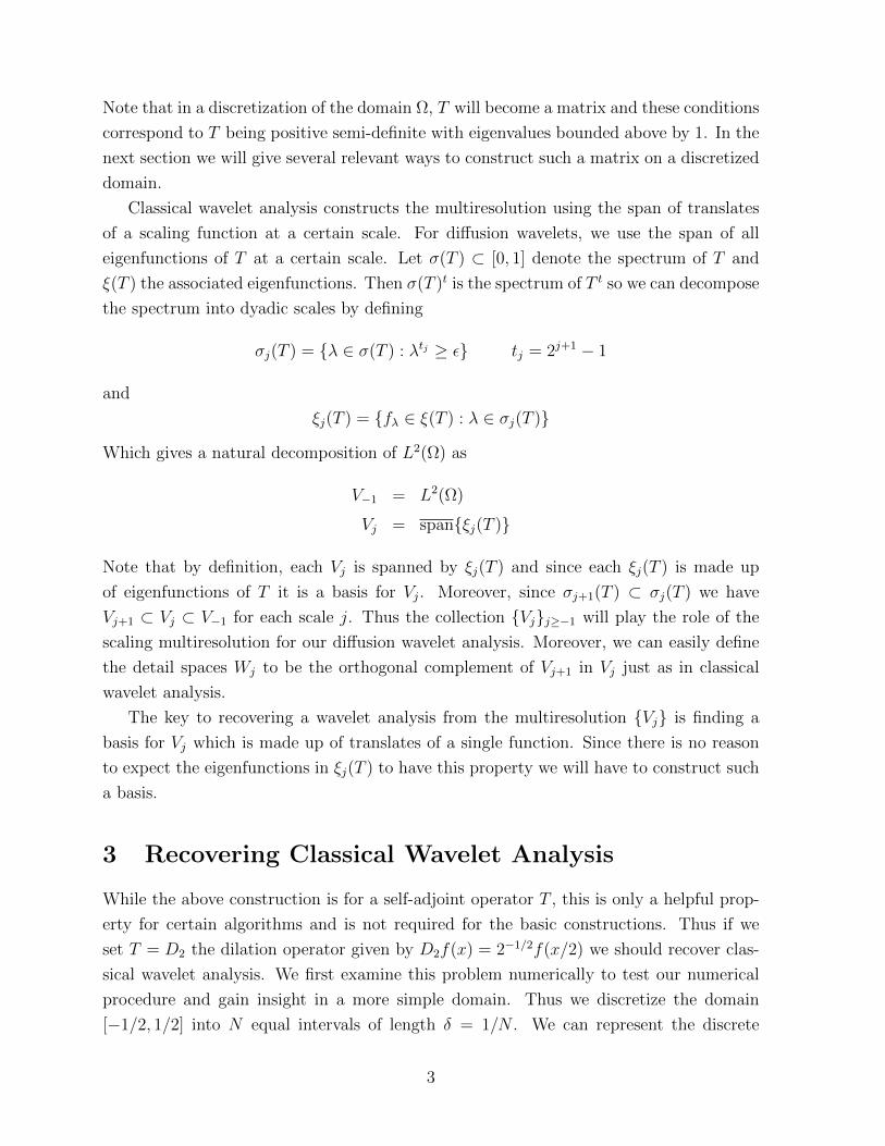
Note that in a discretization of the domain Ω, T will become a matrix and these conditions

correspond to T being positive semi-definite with eigenvalues bounded above by 1. In the

next section we will give several relevant ways to construct such a matrix on a discretized

domain.

Classical wavelet analysis constructs the multiresolution using the span of translates

of a scaling function at a certain scale. For diffusion wavelets, we use the span of all

eigenfunctions of T at a certain scale. Let σ(T ) ⊂ [0, 1] denote the spectrum of T and

ξ(T ) the associated eigenfunctions. Then σ(T )t is the spectrum of T t so we can decompose

the spectrum into dyadic scales by defining

σj(T ) = λ ∈ σ(T ) : λtj ≥ ε tj = 2j+1 − 1

and

ξj(T ) = fλ ∈ ξ(T ) : λ ∈ σj(T )

Which gives a natural decomposition of L2(Ω) as

V−1 = L2(Ω)

Vj = spanξj(T )

Note that by definition, each Vj is spanned by ξj(T ) and since each ξj(T ) is made up

of eigenfunctions of T it is a basis for Vj. Moreover, since σj+1(T ) ⊂ σj(T ) we have

Vj+1 ⊂ Vj ⊂ V−1 for each scale j. Thus the collection Vjj≥−1 will play the role of the

scaling multiresolution for our diffusion wavelet analysis. Moreover, we can easily define

the detail spaces Wj to be the orthogonal complement of Vj+1 in Vj just as in classical

wavelet analysis.

The key to recovering a wavelet analysis from the multiresolution Vj is finding a

basis for Vj which is made up of translates of a single function. Since there is no reason

to expect the eigenfunctions in ξj(T ) to have this property we will have to construct such

a basis.

3 Recovering Classical Wavelet Analysis

While the above construction is for a self-adjoint operator T , this is only a helpful prop-

erty for certain algorithms and is not required for the basic constructions. Thus if we

set T = D2 the dilation operator given by D2f(x) = 2−1/2f(x/2) we should recover clas-

sical wavelet analysis. We first examine this problem numerically to test our numerical

procedure and gain insight in a more simple domain. Thus we discretize the domain

[−1/2, 1/2] into N equal intervals of length δ = 1/N . We can represent the discrete

3

version of L2([−1/2, 1/2]) as vectors y ∈ RN where yi = f(i/N − 1/2). Thus yi is the

representation of f with respect to the basis (for the discrete space of functions) of delta

functions δi = 1x=i/N−1/2. Note that we cannot define D2 exactly on this domain, since

D2(yi) = D2(f(i/N − 1/2) = f(i/N/2− 1/4) but there is no value in our vector y which

represents the point i/N/2− 1/4. Thus we must choose an interpolation scheme, and the

discrete version of D2 will actually represent interpolation followed by dilation. We now

introduce two interpolation schemes which will be used below.

3.1 First Order Interpolation

For a first order interpolation, we simply interpolate linearly between the discrete points

i/N − 1/2. Thus to find D2(yi) = f(i/N/2− 1/4) choose k/N − 1/2 be the closest point

to the left of i/N/2− 1/4. Then, letting m = (i/2− k +N/4) we can approximate

D2(yi) = f(i/N/2− 1/4) ∼=yk+1 − yk

1/N(i/N/2− 1/4) + yk = myk+1 + (1−m)yk

Thus in our matrix representation of D2 we set the (i, k) entry to (1−m) and the (i, k+1)

entry to m. Repeating this for each i gives us a matrix representation for D2 which is

shown graphically in Figure 1. Thus for any function represented discretely as a vector y

we can compute interpolation followed by dilation simply by multiplying y by the matrix

D2. Note that the rows of D2 sum to 1 which guarantees that the eigenvalues are bounded

above by 1 and D2 is positive semi-definite but not symmetric.

Figure 1: Left: Image of the matrix D2 for the first order interpolation, Right: D2 applied

to vector representing a simple function.

To find the scaling functions, we compute the QR-decomposition of D2, which is shown

in Figure 2. The matrix Q represents a change of basis matrix that takes the initial basis

4

of delta functions δi to a basis for V0 which consists of translates of a single function. Note

that since D2 is not full rank, only the left half of the Q matrix in figure 2 is meaningful.

This can also be seen by noticing that R is only non-zero in the upper half of the matrix

as shown in figure 2. Notice that each column of Q represents a scaling function at scale

1 which are all translates of each other and this is reflected in the structure of Q, each

column is simply a shift of the previous column.

Figure 2: The scaling QR decomposition of the operator D2 in figure 1, Left: Q matrix,

Right: R matrix.

To find the wavelet functions we need to repeat the above analysis, but on the or-

thogonal complement of the space V0 in V−1. This is reflected in the fact that the matrix

Q is not full rank, and hence I − QQT spans the space W0 and we can find the wavelet

functions by performing a QR-decomposition

I −QQT = Q1R1

and the columns of Q1 will contain the wavelet functions. This is shown in the left image

of figure 3. As we can see the columns from this matrix are not well localized, which is

due to the right half of Q which is meaningless (shown in figure 2). By setting Q equal

to Q with the right half set to zero we achieved much better results with

I − QQT = QR

In all our results we use wavelet functions coming from the columns of Q. Note that

in figure 3 we can see that Q is well localized and each wavelet function is approximately

a simple translate of a single function. The results in Figure 4 show examples of the first

order scaling functions and wavelets at scale V0. The left image in figure 4 shows that

5

Figure 3: The wavelet decomposition, Q1 (left) such that Q1R1 = I−QQT and the matrix

Q (right) such that QR = 1− QQT

each wavelet is approximately a translate of a single function (note some are inverted,

which can be accounted for by the sign of the corresponding entry in the R matrix from

the QR-decomposition). In the right image in figure 4 we show examples of a scaling

function (red) along with its FFT (red, dotted) and also a wavelet (blue) and its FFT

(blue, dotted).

Figure 4: Left: First Order Wavelets, Right: First Order Wavelet (blue) and FFT (blue

dotted) and Scaling function (red) and FFT (red dotted)

6

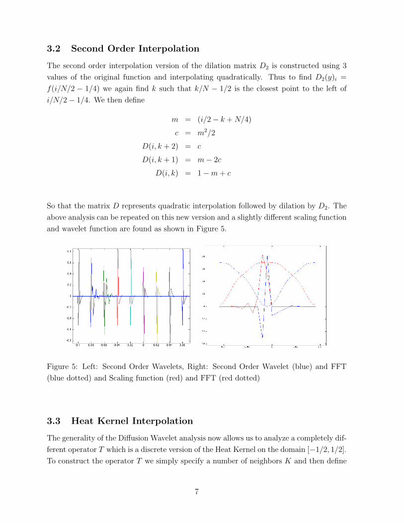
3.2 Second Order Interpolation

The second order interpolation version of the dilation matrix D2 is constructed using 3

values of the original function and interpolating quadratically. Thus to find D2(y)i =

f(i/N/2 − 1/4) we again find k such that k/N − 1/2 is the closest point to the left of

i/N/2− 1/4. We then define

m = (i/2− k +N/4)

c = m2/2

D(i, k + 2) = c

D(i, k + 1) = m− 2c

D(i, k) = 1−m+ c

So that the matrix D represents quadratic interpolation followed by dilation by D2. The

above analysis can be repeated on this new version and a slightly different scaling function

and wavelet function are found as shown in Figure 5.

Figure 5: Left: Second Order Wavelets, Right: Second Order Wavelet (blue) and FFT

(blue dotted) and Scaling function (red) and FFT (red dotted)

3.3 Heat Kernel Interpolation

The generality of the Diffusion Wavelet analysis now allows us to analyze a completely dif-

ferent operator T which is a discrete version of the Heat Kernel on the domain [−1/2, 1/2].

To construct the operator T we simply specify a number of neighbors K and then define

7

the diffusion distance from a discrete point to each of its K nearest neighbors as

T (i, k) = exp−(i/N − k/N)2/σ

Where k is the index of one of the K nearest neighbors of the point indexed by i and σ is

a tuning parameter which is related to the diffusion rate and may need to be adjusted as

the number K of nearest neighbors changes. Note that this distance could be defined for

all points, however it decays very quickly and so a sparse representation of T using the

K nearest neighbors is much more efficient. Finally the columns of T are normalized to

sum to 1.

The above analysis was repeated for the matrix T in order to construct the scaling

and wavelet functions. Again they were found to be approximately translates of a single

function and the results are shown in Figure 6.

Figure 6: Left: Heat Kernel Wavelets, Right: Heat Kernel Wavelet (blue) and FFT (blue

dotted) and Scaling function (red) and FFT (red dotted)

4 Image Analysis

Images are very high dimensional, however, restricted to a particular domain, such as

images of faces, only a small portion of the high dimensional space contains data. A

common personal camera can now produce 2048-pixel by 1024-pixel images, with at least

3 vales (red, green, and blue) per pixel. If we assume that these values lie in I = [0, 1]

then a priori such an image is a point in I6,291,456. Of course we are not interested in the

entire set of images, but a subset. For example if we are only studying images of faces, we

can consider the space A ⊂ I6,291,456 of all face images. Moreover, a smooth perturbation

of a face image will usually still look like a face and thus should lie very near the space

8

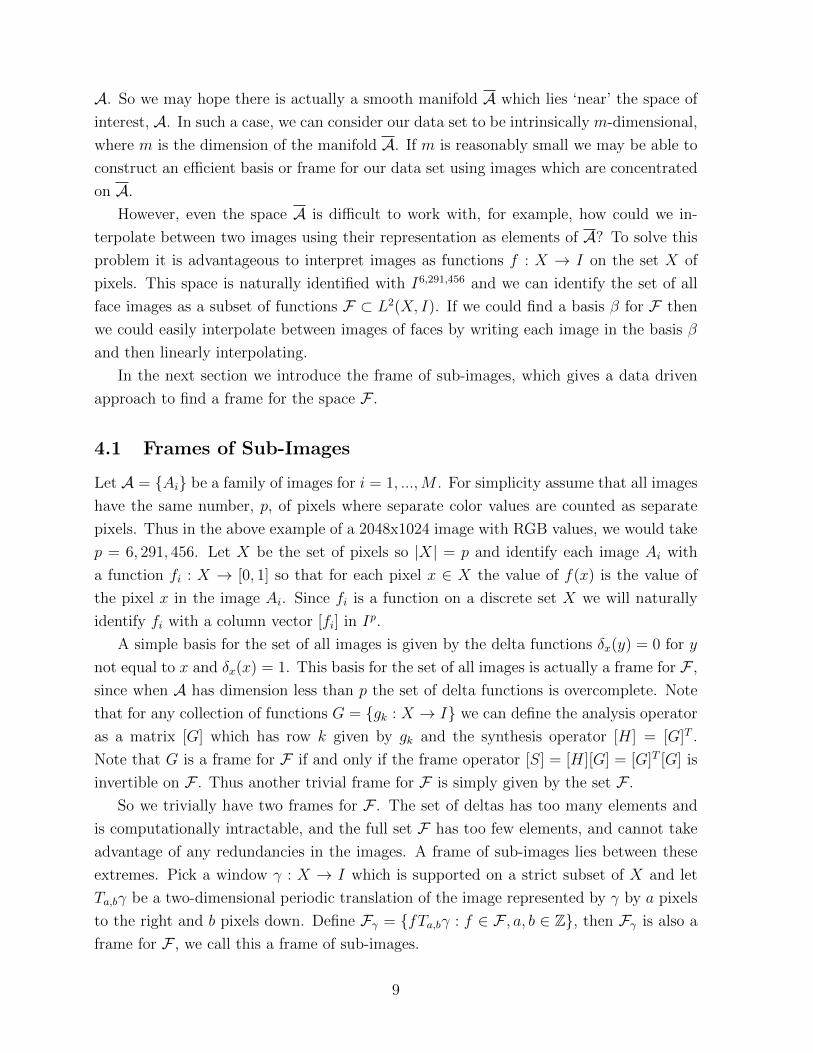
A. So we may hope there is actually a smooth manifold A which lies ‘near’ the space of

interest, A. In such a case, we can consider our data set to be intrinsically m-dimensional,

where m is the dimension of the manifold A. If m is reasonably small we may be able to

construct an efficient basis or frame for our data set using images which are concentrated

on A.

However, even the space A is difficult to work with, for example, how could we in-

terpolate between two images using their representation as elements of A? To solve this

problem it is advantageous to interpret images as functions f : X → I on the set X of

pixels. This space is naturally identified with I6,291,456 and we can identify the set of all

face images as a subset of functions F ⊂ L2(X, I). If we could find a basis β for F then

we could easily interpolate between images of faces by writing each image in the basis β

and then linearly interpolating.

In the next section we introduce the frame of sub-images, which gives a data driven

approach to find a frame for the space F .

4.1 Frames of Sub-Images

Let A = Ai be a family of images for i = 1, ...,M . For simplicity assume that all images

have the same number, p, of pixels where separate color values are counted as separate

pixels. Thus in the above example of a 2048x1024 image with RGB values, we would take

p = 6, 291, 456. Let X be the set of pixels so |X| = p and identify each image Ai with

a function fi : X → [0, 1] so that for each pixel x ∈ X the value of f(x) is the value of

the pixel x in the image Ai. Since fi is a function on a discrete set X we will naturally

identify fi with a column vector [fi] in Ip.

A simple basis for the set of all images is given by the delta functions δx(y) = 0 for y

not equal to x and δx(x) = 1. This basis for the set of all images is actually a frame for F ,

since when A has dimension less than p the set of delta functions is overcomplete. Note

that for any collection of functions G = gk : X → I we can define the analysis operator

as a matrix [G] which has row k given by gk and the synthesis operator [H] = [G]T .

Note that G is a frame for F if and only if the frame operator [S] = [H][G] = [G]T [G] is

invertible on F . Thus another trivial frame for F is simply given by the set F .

So we trivially have two frames for F . The set of deltas has too many elements and

is computationally intractable, and the full set F has too few elements, and cannot take

advantage of any redundancies in the images. A frame of sub-images lies between these

extremes. Pick a window γ : X → I which is supported on a strict subset of X and let

Ta,bγ be a two-dimensional periodic translation of the image represented by γ by a pixels

to the right and b pixels down. Define Fγ = fTa,bγ : f ∈ F , a, b ∈ Z, then Fγ is also a

frame for F , we call this a frame of sub-images.

9

We now give an example of a frame of sub-images and the frame reconstruction on a

space A of images of faces. We take a window function γ which is 1 on a 4-pixel by 4-pixel

square in the middle of the image and zero everywhere else. Thus the product fTa,bγ is

literally a sub-image of the full image f . Each image Ai ∈ A will be a simple 32x32 RGB

image of a face a shown in Figure 7. Thus each image can be represented as a vector of

length 3072 (32x32 with 3 values at each location).

Figure 7: Left: Example images of faces from A, Right: left column shows original face

images, middle column shows the frame operator applied to the image, right column shows

the reconstructed face image (this format is used repeatedly below).

In this example we only took 16 images for our space A and instead of forming the

full frame Fγ we chose 4096 random translations. Since the images are at most 3072-

dimensional it was reasonably certain that 4096 images would give a frame, and indeed

the frame operator was invertible. In Figure 7 this is clearly shown as images had very

good reconstruction after the applying the frame operator. Even more impressive, this

seems to be a good frame for the set of all such face images since Figure 8 shows that

even faces which were not included in the initial set A could still be reconstructed after

the frame operator was applied.

Next we applied the same analysis with only 1024 random translations of the window.

Since the full image space is 3072-dimensional this cannot be a frame for the full image

space, however it may still be considered a frame for the space of facial images. Note that

images of faces in Figure 9 are not perfectly reconstructed, viewed as an image they are

noisy, however viewed as a face this reconstruction may be considered exact depending

upon the precise definition of a face. Note, also in Figure 9, that on images of non-faces

the performance degrades significantly.

10

Figure 8: Frame operator and reconstruction applied to out-of-sample faces.

Figure 9: Left: Good reconstruction for faces, Right: Poor reconstruction for non-faces.

11

Finally, we attempted a reconstruction using only 512 random translations and per-

formance degraded considerably as shown in Figure 10 but faces are still somewhat rec-

ognizable.

Figure 10: Left: Good reconstruction for faces, Right: Poor reconstruction for non-faces.

Note, in Figure 11, that even partial faces are reconstructed, while the non-face parts

of the image are drastically changed.

This pragmatic approach to constructing a frame for a space of images uses sub-images

(defined by the translates of the window γ) to build a frame. It is clear that if enough

such sub-images are chosen the result will be a frame, however our experiments show that

even for a relatively small number of randomly chosen sub-images the behavior is similar

to a frame in that approximate reconstruction is possible. In face these small sets are

frames for some space (their span) which is a reasonable approximation of the space Awhich we wish to represent.

12

Figure 11: Reconstruction of partial face images.

4.2 Multiscale Image Distance

Let A = Ai be a family of images for i = 1, ...,M . Our first goal is to produce a

multi-scale distance on images following [2]. We begin by defining a distance on the sub-

images. Let XijNj=1 be the collection of all 5-pixel by 5-pixel sub-images of Ai. Note

that Fγ = Xiji,j as defined in Section 4.1. For simplicity we assume that all the images

are the same size so N does not depend on i.

Each sub-image has 16 pixels with 3 color values and so we can represent it as a 48

dimensional vector. Each sub-image also has a 2-coordinate location in it’s source image,

which we denote (xij, yij). Following [2] we let Yij = (Xij, xij, yij) be a 50-dimensional

vector created by appending the sub-image location to the 50-dimensional representation

of each respective sub-image. Next we define a distance on the space of sub images by

d(Yij, Ykl) = ||Xij −Xkl||2 + σ√

(xij − xkl)2 + (yij − ykl)2

We will explore the role of the parameter σ in later sections. For convenience, we choose

an ordering of the sub-images Yr using a single index.

To define a diffusion operator on the space of images A we first define the operator

on the set of sub-images Fγ. Essentially we define a random walk on the space of sub-

images, so the the translation probability between any two sub-images is proportional

13

to exp−d(Yr, Ys)/κ. Note that when the distance d(Yij, Ykl) is large the probability

is essentially zero, thus we can save memory by defining a sparse matrix T such that

Trs = exp−d(Yr, Ys)/κ for s ranging over the k-nearest neighbors of Yr and Trs = 0

otherwise.

Note that as long as the set of sub-images Ys is a frame for the set of images, we

can use T to define a multi-scale distance on the set of all images by setting

ds(Ai, Ak) = ||T qGfi − T qGfk||2

where fi, fj the function representations of the images Ai and Aj respectively and G is the

frame operator as defined in Section 4.1. In the next section we use the diffusion operator

on the space of images to build Diffusion Wavelets using the technique from Section 2.

4.3 Wavelets for Spaces of Images

With the above construction of a diffusion operator T we can proceed according to the

construction in Section 2 to find Diffusion Wavelets. In general these wavelets will depend

on the size of the sub-images (or more generally on the window γ defined in Section 4.1)

and also on the parameter σ defined in Section 4.2. In Figures 12 and 13 we show examples

of scaling functions and wavelets.

Figure 12: Diffusion Scaling Functions on the space of face images.

14

Figure 13: Diffusion Wavelets on the space of face images.

5 Bibliography

[1] R. Coifman and S. Lafon, Diffusion Maps, Applied and Computational Harmonic Analysis

21 (2006), 5-30.

[2] R. Coifman and M. Maggioni, Diffusion Wavelets, Applied and Computational Harmonic

Analysis 21 (2006), 53-94.

[3] R. Coifman, J. Bremer, M. Maggioni, and A. Szlam, Biorthogonal diffusion wavelets for

multiscale representations on manifolds and graphs, Proc. SPIE 5914 (2005).

[4] A. Szlam, R. Coifman, J. Bremer, and M. Maggioni, Diffusion-driven multiscale analysis on

manifolds and graphs: top-down and bottom-up constructions, Proc. SPIE 5914 (2005).

[5] V. Garcia and E. Debreuve and M. Barlaud, Fast k nearest neighbor search using GPU,

CVPR Workshop on Computer Vision on GPU, 2008.

[6] Gary B. Huang and Manu Ramesh and Tamara Berg and Erik Learned-Miller, Labeled Faces

in the Wild: A Database for Studying Face Recognition in Unconstrained Environments 07-

49 (2007).

15