Tina Memo No. 2002-008Internal Report

Diagnosis of Dementing Diseases through the Distributionof Cerebral Atrophy: Development of a Multi-Objective

Evolutionary Algorithm Optimiser

P. A. Bromiley and N.A. Thacker

Last updated1 / 7 / 2002

Imaging Science and Biomedical Engineering,School of Cancer and Imaging Sciences,

University of Manchester, Stopford Building,Oxford Road, Manchester M13 9PT, U.K.

Diagnosis of Dementing Diseases through the Distribution

of Cerebral Atrophy: Development of a Multi-Objective

Evolutionary Algorithm Optimiser

P.A. Bromiley and N.A. ThackerImaging Science and Biomedical Engineering,

School of Cancer and Imaging Sciences,University of Manchester, Stopford Building,Oxford Road, Manchester M13 9PT, U.K.

paul.bromiley@man.ac.uk

Abstract

This report describes the development of a multi-objective genetic algorithm within the TINA machinevision software. This algorithm is intended to be used to optimise the diagnostic capabilities of thedementing disease diagnosis technique described in [23]. Many features previously described in the lit-erature are incorporated: the use of a secondary population, mating restriction, random immigration,and deterministic crowding. However, a novel mating restriction is used in order to prevent global con-vergence in the primary population, such that the primary population searches the space indefinitely.Convergence is performed exclusively in the secondary population. This division of searching and con-vergence across two populations avoids the difficulties commonly associated with the trade-off betweenthese two behaviours, such as premature convergence, but without applying features that artificiallyenforce diversity in the population (e.g. fitness sharing) or require problem-specific adjustments (e.g.annealing schemes). The algorithm is compared to four other algorithms incorporating fitness sharing,and is shown to produce a better estimate of the Pareto front over a range of real-valued multi-objectivetest problems.

1 Introduction

A previous publication [23] described a technique capable of diagnosing a number of dementing diseases throughanalysis of the distribution of cerebral atrophy in MRI scans. In brief, the technique divides the interior of thecranium into twelve volumes (anterior, middle and posterior thirds, plus horizontal and vertical dividing planesplaced centrally) and counts the number of pixels containing CSF in each. These quantities are then normalised forhead size, through division by the total volume, and for age-related atrophy, assuming a simple inverse proportionalrelationship. Finally, the twelve normalised variables are combined to produce five relative variables. This techniquehas been applied to a study group incorporating normals, Alzheimers Disease, Fronto-Temporal Dementia andVascular Dementia. Projected plots of the 5D space show good separation of these groups, and the results fromapplying a cross-validated Parzen classifier indicated that the four disease groups could be diagnosed with anaccuracy of around 80%.

The previous work can be considered as a proof of concept, indicating that relatively crude measures of cerebralatrophy can produce useful diagnostic information, whilst avoiding the complexities of non-rigid co-registrationand segmentation that would be introduced in any attempt to produce accurate atrophy maps. Having illustratedthe viability of such techniques, it seems natural to attempt to optimise the diagnostic capabilities. In particular,the definition of the twelve boxes used in the CSF counting is sub-optimal, since the box sizes approximatethe underlying structure of the brain on the coarsest scale (division into lobes) and yet ignore this information.Therefore, it seems reasonable to attempt to optimise the placement of the decision boundaries to maximisediagnostic capability. The processor time required to compute the relevant cost function over any reasonably sizedpatient group precludes the use of exhaustive search. Little is known about the form of the cost function: it maybe non-smooth and discontinuous, and first differentials will not be available. Since the optimisation must beperformed over a number of diseases, and using enough example data sets to guarantee generalisation capability,a multi-objective optimisation routine that does not use differentials is required.

Of the multi-objective optimisation techniques described in the literature, the multi-objective genetic algorithmseems most applicable to the task at hand. Such algorithms are modelled on the process of evolution, using

a population of candidate solutions to explore the space, combining information from the solutions to generatebetter solutions, and incorporating survival of the fittest to promote convergence. The basic element in this caseis the individual: each contains a chromosome that encodes the position of a point in the space defined by the costfunctions. A population of random individuals is set up, and then pairs of individuals are selected for breeding.During breeding, genetic information from the parents is recombined in some way to generate children. Randommutation is applied to the child chromosomes. The children are then evaluated against their parents (in termsof the cost function) and the weakest are replaced (the fittest are retained) in the population ready for the nextround of breeding. All evolutionary algorithms incorporate these four features (selection, crossover, mutation andreplacement) in some way. At the crudest level, crossover allows the best features from a chromosome pair to becombined, such that the children may inherit the strengths of each. Mutation ensures that some random searchingof the space occurs. Replacement ensures convergence. Selection is more subtle and can influence the progressof the algorithm in a number of ways, such as speeding convergence by allowing the fittest individuals to breedmore often. It should be recognised that the literature describes a wide range of variations on each of these steps.Since the first genetic algorithms were implemented in the mid-eighties [7, 18], over 450 publications [3] havedescribed various implementations, applications and, to a lesser extent, underlying theory. Several reviews existin the literature e.g. [5, 8, 25] and so no attempt will be made to provide an exhaustive survey here.

In single objective optimisation, the desired result is usually one or more global and/or local optima. Ideallythe cost function should be defined on the basis of quantitative statistical principles, derived from a probabilisticspecification of the task [22]. However, in many practical problems we need to take into account several factors thatcannot be easily combined into a single simple objective. Such non-commensurate objectives require approachesthat can optimise multiple objectives simultaneously and independently. The transition to multiple objectives canbe handled in several ways [6]. For instance, a weighting scheme can be used to combine the objectives into a singlevalue. However, the solution then becomes sensitive to the values of the weights. These can be randomly varied,or as an alternative the search can be directed to each objective in turn, or the objectives can be ranked in order ofpreference and optimised in turn, but in general all such techniques are unsatisfactory or at best problem-specific.

It is possible to demonstrate these relational difficulties using probability theory, in order to arrive at some gen-eral conclusions regarding what might be achieved in such problems. To form a conclusion within a hypothesisframework, a single probability relating to the best hypothesis is required. Given a set of objectives ai and somehypothesis H , the probabilities of the hypothesis given the ai could be calculated by making certain assumptions A.Then, assuming that these probability functions were available and were statistically independent, their productwould give the required single, overall probability

P (H |a, A) =∏

i

P (H |ai, A) (1)

If, however, the P (H |ai, A) were kept separate a space of candidate solutions formed, we would expect to findthat the space had a bounding surface featuring cusps and ridges corresponding to local extrema in the combinedobjectives. It would be these locations that would produce the local and global optima of the combined function.

In practice, for the majority of multi-objective problems, the P (H |ai, A) will not be available, and only the ai

will be known. In addition, the P (H |ai, A) may not even be independent, producing a rotation of the axes ofthe space of P (H |ai, A) (the probability space). This dependency may even vary across the space of the ai (theobjective space), making it very difficult to ever be able to formulate a simple strategy back to the probabilisticinterpretation. Also, the required set of assumptions A may be ambiguous or even impossible to define. Therefore,in general, distances and geometry in the objective space are largely meaningless. However, in general the ai willbe monotonically related to the probability space (a one-to-one mapping).

P (H |a, A) = fi(ai) (2)

Since we expect diffeomorphic equivalence between the probability and objective spaces, ridges (local peaks in onedimension) and cusps (local peaks in two or more dimensions) in P (H |ai, A) are still ridges and cusps in ai, andwe would expect to find useful global optima around these positions. These positions in the parameter space definethe Pareto-front and it is this front that we wish to locate when we use a multi-objective genetic algorithm. It isclear therefore that the assumptions required to transform between these spaces specify a certain trade-off betweenthe objectives, and that the theoretical global optimum in the probabilistic space corresponds to a point on thePareto front in the objective space, generally around the cusps (since these represent extrema in one of the ai

on the Pareto front). Therefore, the output from a multi-objective evolutionary algorithm must contain multipleoptima, which sample all possible optima that could have been candidates for the theoretical global optimum werethe required assumptions available. We will explicitly define this as the goal in our work.

3

Since the desired goal in multi-objective optimisation is to produce a number of optimal solutions spanning thePareto front, the use of a genetic algorithm conveys an immediate advantage in that such algorithms necessarilymaintain a large population of solutions and so can capture the entire range of the Pareto front in a single run.However, they also convey a second, more subtle, advantage. As long as the population does not become degenerate,several optimisation strategies are available. The most powerful of these is the combination of “building blocks”[9], optimised sub-sections of chromosomes, from individual solutions to produce fitter solutions. If this strategy isnot available, the algorithm will decay in turn to stochastic hill-climbing and finally random search. This behaviourguarantees that, given infinite computational resources, global optima will always be found. It is therefore relativelyeasy to produce a naive genetic algorithm that simply implements crossover, mutation and patricide and locatesthe global optima eventually. In addition the “No Free Lunch” theorems [28] state that an genetic algorithm mustincorporate problem-specific knowledge in order that a formal statement about general effectiveness can be made,and so there is no such thing as a “best” genetic algorithm. However, testing on a broad range of test functions,chosen to exhibit a range of behaviours, should be enough to indicate the potential of an genetic algorithm.

One of the main issues facing any optimisation routine is striking a tradeoff between the diametrically opposedobjectives of searching and convergence. An important aspect of this problem in the case of multi-objectiveoptimisation using an genetic algorithm is maintaining the population diversity. When presented with multipleoptima a naive genetic algorithm will still converge onto a single solution, due to three effects: selection pressure,selection noise, and operator disruption [14]. This phenomenon, known as genetic drift, has been seen in naturalas well as artificial evolution [6]. A wide range of mechanisms known collectively as niching, sharing and crowdingmethods exist to maintain the diversity of the Pareto front [14]. A popular example is fitness sharing [11], whichessentially penalises the fitness values of solutions in close proximity to each other.

The multi-objective genetic algorithm literature describes a wide variety of diversity preservation strategies. How-ever, these modifications also often require additional arbitrary parameters in order to control the search andconvergence of the algorithm, in addition to key parameters such as population size and the probabilities governingthe application of operators such as mutation and crossover. Unfortunately, these parameters often need tuningto each specific optimisation problem. In addition, the design choices made for the construction of an algorithmwill have implications regarding the ideal formulation of optimisation problems, for example the construction ofchromosomes. One goal of this work was therefore the specification of a search strategy that efficiently identifies ofthe Pareto-front with a minimum number of control parameters, and an understanding of efficiency from the pointof view of problem formulation. In particular we will show how to eliminate the need for accurate determinationof population size and arbitrary parameters to reduce crowding, and the characteristics a chromosome must havefor efficient search.

To rephrase the problem, we desire an algorithm that will search the space globally to identify promising regions ofthe cost function, but converge locally within these regions to find the optima. The analogy of speciation in naturalevolution immediately suggests itself, leading to the concept of restricted mating. A wide range of variations onthis theme have been used in the past [14], restricting mating so that it only occurs between similar (or dissimilar)individuals. However, unless the population is divided into separate species that are never allowed to interact,convergence will be delayed rather than prevented and collapse to a single point will still occur.

The approach taken here is quite different and relies upon novel use of several features found in previous work:the use of a secondary population to store the non-dominated individuals found so far; random immigration(i.e. introducing new random individuals into the population); and restricted mating, using a novel criterionthat allows mating only between neighbouring individuals. The concept is to enforce the differentiation of globalsearching and local convergence. We consider the primary population as a tessellation of the search space withVoronoi cells [27], and by allowing mating only between Voronoi neighbours enforce the algorithm’s own naturaldefinition of local/global. Additionally, we extract individuals from the primary population if they have undergonesome number of attempts at mating without producing fitter children (“static extraction”), and place them in asecondary population, which is sorted such that it contains the current non-dominated set of extracted individuals.The extracted individuals are replaced by random immigrants, such that the primary population size remainsconstant. We demonstrate that this prevents any general convergence of the primary population, thus dividing theprocesses of searching and convergence over the primary and secondary populations respectively. It also extendsany initial definition of the population size in time so that, beyond a minimum size necessary to maintain a breedingpopulation across the space, the population is potentially infinite. This therefore removes this free parameter fromthe specification of the algorithm. We test the algorithm on a range of single and multi-objective test problemsfound in the literature, and show its performance to be at least equal to a range of other genetic algorithmspreviously described.

As a final note, it is important to stress the differences between genetic algorithms that use binary and real-valuedrepresentations. In the first case, the analogy with a biological chromosome, and thus the meanings of crossover

4

and mutation, are more obvious. Crossover can be performed by taking the string of bits encoding each parent,splitting them at some point, and swapping over the information below that point, and mutation can be performedby flipping a single bit. On a more subtle level, the number of solutions within a constrained space is countable,and there exists a simple definition of identicality that can be used in various ways. However, in order to representa real-valued problem in binary form some loss of accuracy must be accepted. The length of the binary string canalways be increased to improve this accuracy, but it has been shown [10] that even for simple problems the requiredpopulation size is of order of the string length. Conversely, real-valued representations can be arbitrarily accurate,and allow the calculation of distances within the space. However, the definitions of mutation and crossover becomeproblematic. In previous work we defined a genetic algorithm for the design and routing of 3D hardware, whichis formulated as a binary search problem [12]. The algorithm presented here can be seen as an extension of thatwork and uses a real-valued representation, no further investigation of the tradeoffs between binary or real-valuedrepresentations will be made.

2 Method: Implementation

The algorithm presented here incorporates the following features. It uses two populations: the primary populationand the extracted set. Upon initialisation, the primary population is filled with a fixed number of randomly-generated solutions, which thereafter remains constant. The solutions are held in data structures called genomes,which contain a set of header information and a list of points encoding the position of the solution in the costfunction space. The header information contains a number of fields for monitoring the progress of each genome,as well as genetic information such as mutation probabilities.

The algorithm then runs through a loop that includes selection, crossover, mutation, patricide, and extractionmanagement. Each loop breeds one pair of solutions, with children directly replacing their parents (rather thancompeting with the entire population). Algorithms of this type have been referred to in the literature as steady-state genetic algorithms, as opposed to generational genetic algorithms where the entire population is paired andbred at each step. In order to aid comparisons with such algorithms, the word “generation” will henceforth be usedto describe a number of executions of the main loop equal to the population size. In addition, allowing childrenonly to replace their own parents, through a fitness competition, has been referred to as deterministic crowding[14]. Some comments on the limitations imposed by combining deterministic crowding with mating restrictionsare included below.

2.1 Selection

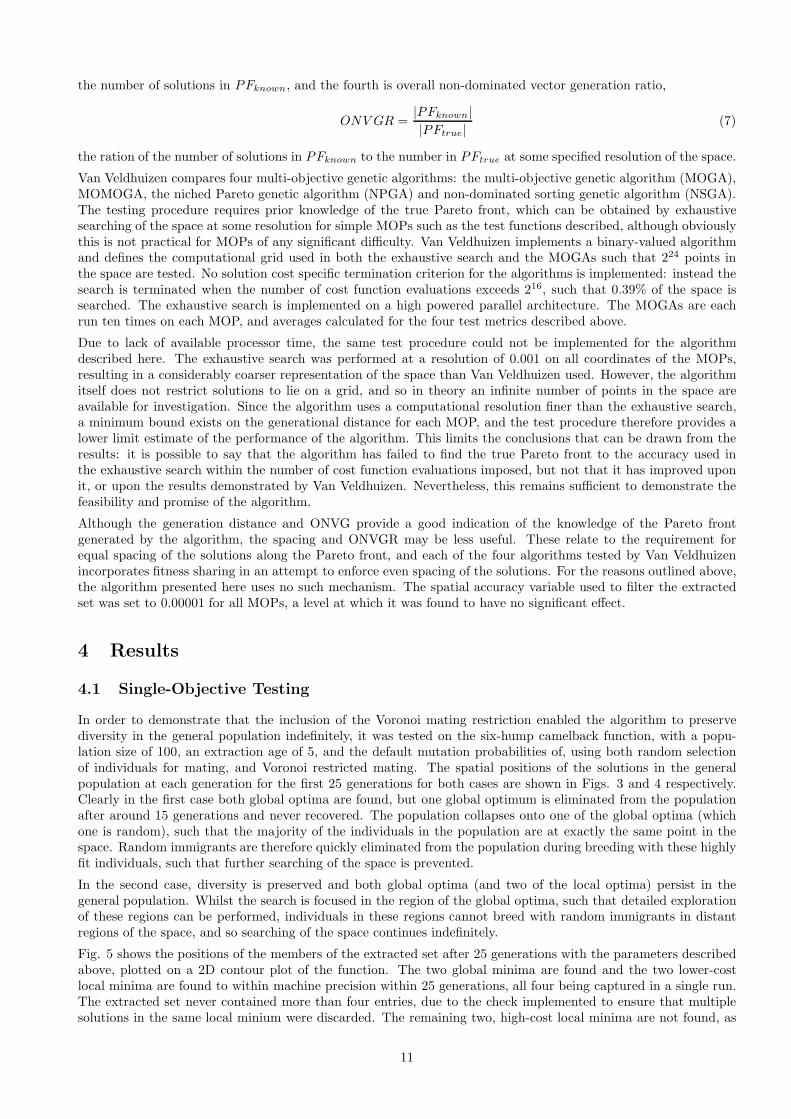
Selection is restricted but random within a subset of the population. Considering the population as a tessellationof the search space with Voronoi cells, mating is restricted to within sets of neighbours. A simple restrictioncriterion was derived to reject pairings that did not involve neighbours [2]. Referring to Fig. 1, if the pairing AB

was being considered, it was compared to all other pairings involving the same first point e.g. AC. The planesbisecting the vectors linking the points are necessarily the Voronoi boundaries if no intermediate cells lie betweenthe individuals. Therefore, if the plane bisecting AC intersects AB (point I) at less than half of its length (to themid-point M), AB must cross an intermediate cell. The angle AB 6 AC is given by

θ = cos−1 AB.AC

| AB || AC | .

Making use of the fact that AI is the hypotenuse of a right-angled triangle, the condition for a pairing to berejected is

| AM |>| AI |⇒ 1 >| AC |2

(AB.AC).

Selection was then performed by randomly selecting a first parent, and then looping over randomly selected secondparents until a Voronoi neighbour was found. The parent pair was then passed on to the later stages (crossoveretc.).

2.2 Crossover

For the test problems described here, each genome encoded a single, real-valued point. Therefore, the definition ofcrossover became problematic, since there was no obvious justification for crossing over sub-sets of the coordinates

5

of a pair of points to generate children. Several crossover operators for use on such representations have beensuggested in the literature (see refs. in [15]). We implemented one of the simplest: child points were placedrandomly within a hyper-cuboid with edges parallel to the axes of the space defined by placing the parent pointsat diametrically opposed corners.

In order to complete each child genome, the header information had to be generated. The only fields over whichthere was any choice were the mutation probabilities, and no crossover was attempted on these. Each childrandomly picked up the entire relevant portion of the header from one of the parents.

2.3 Mutation

In binary representations, mutation can be implemented by flipping a single bit in the genome, thus introducinga limited amount of change. All that is required is a probability of mutation. In real-valued representations, thesituation is more complex as a definition of a “limited” amount of change is required in addition to the mutationprobability. Although the literature contains suggestions of suitable mutation probabilities (e.g. [1], there seems tobe little theoretical justification. Therefore, we took an alternative approach of using the GA to optimise its ownmutation parameters. The header for each genome contained five pieces of mutation information: the probabilitythat breeding would occur with no crossover, only mutation; the probability that, after crossover, there would bea mutation in the header; the probability that, after crossover, there would be a mutation in the spatial positionof the genome; the maximum distance (as a proportion of the total width of the space) by which a coordinatewould be changed if mutated; and the maximum amount (in terms of probability) by which a mutation probabilitywould be changed if mutated. Default values were 0.5, 0.5, 0.2, 0.1 and 0.1 respectively. Since these quantitieswere placed in the header and could themselves be mutated, they could be optimised by the GA itself.

It should be noted that the mutation probabilities in the header did not influence the fitness of a genome in thesame way as its spatial position in terms of the cost function. The latter was a direct effect: the position of agenome in the space implies values of the cost function, which in turn determine whether it survives to breed.The mutation probabilities determined in part the probability that a genome would generate children that wouldgo on to breed, and so were one step removed from directly influencing the fitness. For this reason, optimisationof the header information was slower than optimisation of the cost function. It was expected that optimisationby crossover would be more efficient at points far from optima, since it would allow rapid movement, whereasoptimisation by mutation would be more desirable close to optima, where it would allow detailed local randomsearching. The meaning of “optimal” for header information was therefore linked to the spatial position of thegenome in terms of the cost function. Therefore, although the initial random population was assigned initialisationheader information entered by the user (typically 0.5 for the probability of breeding by crossover and 0.1 for allother values), once the main loop had begun, randomly generated genomes were given random spatial positions,and then copied header information from the spatially nearest genome in the population, based on a Euclideandistance measure. This encouraged the optimisation of header information. It also had a biological analogue 1.

2.4 Patricide

The patricide stage involves comparison of the children with the parents in terms of the cost function, implementingsurvival of the fittest. The cost function is evaluated for both children, and their costs compared with the parents.Two versions were implemented. The first involves a “first come, first served” principle. A loop over the parentscontaining a nested loop over the children was used to compare both children with both parents, replacing a parentwith a fitter child as soon as such a combination was found. However, a situation could arise in which the firstchild was fitter than both parents, but the second child was only fitter than the first parent. In this situation, thefirst child would replace the first parent before the second child was tested. The second child would not then beable to replace the second parent, and so would be discarded. In order to avoid this behaviour, a maximally child-preserving patricide routine was also implemented that tested all possible combinations of children and parents,and sorted the replacements so that as many occurred as possible. However, this added complexity was found tobe unnecessary in practice, and so the simple patricide routine was used.

Since the cost function encoded multiple objectives, a definition of a child being “better than” a parent wasrequired. It was not sufficient to look for children that beat a parent on any single objective, since this could leadto oscillatory behaviour: a child could replace its parent on objective A whilst getting worse on objective B, thenthe child might breed to regenerate the parent, which would replace the child on objective B whilst getting worseon objective A, and so on. In order to avoid this, a vector of binary direction flags was encoded in the header of

1Many species of bacteria are able to exchange genetic information in a similar way, allowing them to rapidly assume genotypessuited to local conditions.

6

each genome, which listed the objectives on which the genome had beaten its parents (but was set to all zeros forrandomly generated genomes). In order to replace its parent, a genome had to optimise on the same objective(s)as the parent, although additional objectives could be added if the child started to optimise on more objectivesthan the parent had done.

The patricide function also included the possibility of a second pass through the breeding and mutation stages.If the parents had bred by crossover, but had failed to generate children that replaced them, then breeding wasrepeated through the cloning/mutation of spatial position route, and patricide was repeated on the new children.This was implemented in order to encourage random searching by mutation for solutions close to an optimum,allowing detailed refinement of such solutions. The final step in the patricide routine was the updating of the agesof the genomes. The term “age” here refers to the number of times that a genome has bred without producingchildren that replaced it, and this quantity was used in the extraction management function described below.

Allowing children to replace only their own parents in the population has been described in the literature asdeterministic crowding [14]. Many crowding mechanisms have been proposed in the past, with the aim being toreplace the most similar elements in the population. This is a diversity preservation strategy, as it prevents highlyfit individuals near the minima of the cost function eliminating less fit individuals elsewhere in the space.

2.5 Extraction management

Following the patricide stage, the breeding pair pointers, which might point to children that had replaced theirparents, was passed to the extraction set manager. The age of each genome was tested against a fixed extractionage, which was typically set to 5-10 breeding attempts. If the genome was older than this, it was extracted from thepopulation and replaced with a randomly generated genome. This is similar to the diversity-preserving strategyknown as “random immigration”, which has previously been described in the literature.

The algorithm was implemented in such a way that the number of objective functions was completely variable.Therefore, although it could be set to any number of multiple objectives, it could also be set to 1 for single-objectiveoptimisation. All of the preceeding stages in the algorithm could cope with either scenario, but the desired outputin the extracted set was different in each case. For single-objective optimisation, we desire (at least) a single globaloptimum, or possibly a list of global optima if more than one exist. Arguably, we might also desire the list to containall local optima, providing additional insight into the behaviour of the cost function, although the list should besorted such that the first member is a global optimum. We would not want the list to contain multiple copiesof essentially the same solution. Since the algorithm presented here used a real-valued representation, a simpledefinition of identicality was not available. However, it is inevitable that the representation used would imposesome accuracy (typically the root of the smallest number that could be represented as a double type variable)[16] and so we are justified in reducing this accuracy in order to provide a distance measure as a definition ofidenticality.

In the case of single-objective optimisation, simply discarding “identical” solutions (always keeping the one withthe lowest cost) is not sufficient to produce a list containing only local (and global) optima. On adding a newsolution to the extracted set, any solutions added in pervious breeding rounds, in the same local minimum, but ata distance greater than the distance used to define identicality, would not be discarded. Therefore, an additionalconstraint was introduced to determine if a solution lay in the same local “valley” in the cost function as anothersolution already in the extracted set. The extracted solution was compared to all solutions in the extracted set,and the cost function at the average of the two positions was calculated. If, for any comparison, the cost at themean was lower than the cost of either of the genomes, then the new genome lay in the same local valley in thecost function as the member of the extracted set against which it had been compared. In that case, the better ofthe two genomes was placed in the set, and the worse discarded. Of course, a situation could arise in which bothgenomes lay in different valleys, with a third valley in between at the position of the mean, leading to a genuinenew local optima being discarded. However, one of the convenient properties of a GA is that, by the time a givensolution is generated, the genetic information required to produce it is usually present in partial form in severalindividuals in the population, and so the solution will be regenerated multiple times, and will rapidly get added tothe population. In addition, on functions that exhibit minima with complex shapes, such as the long, thin, curvedminima of the Rosenbrock’s Valley function [17], this method will still allow multiple solutions in the valley to beadded to the extracted set.

There is one remaining situation in which local optima might never get added to the extracted set, illustrated bythe six-hump camelback function described below. This function has six local optima, two of them global. Twoof the local optima have costs relatively close to the global optima (compared to the range of the function) buttwo have relatively high costs. These high-cost local optima were never added to the extracted set, since there arepoints on the function outside the local valley, but still relatively close, with lower costs. Therefore, the high-cost

7

local optima tend to get replaced by children before they can be extracted. This behaviour could in theory beprevented by reducing the extraction age to a very low value, but this would degenerate into a random search.However, it is arguable that high-cost local optima would never be desired in the output from an optimisationroutine, and so this behaviour was not considered to be a serious drawback.

In the case of multi-objective optimisation, the extracted set should contain a good representation of the Paretofront i.e. solutions spread along the whole length of the front. In the literature, this has sometimes been interpretedas meaning that the solutions should be evenly distributed along the front, and performance metrics measuringthe uniformity of this distribution have been suggested [20, 19]. However, it is arguable that this idea contains afundamental flaw, since it assumes that all non-dominated solutions are equally desirable. In fact, as explainedin our discussion of the relationship of the Pareto-front to probability theory, this may not be the case. Solutionsclose to the ends of the Pareto front, or on cusps in the front (in cost function space) can be more valuable asthey represent the best attainable performance on one of the cost functions (at the expense of the others). Toparaphrase Orwell, all non-dominated solutions are equal, but some are more equal than others. The GA presentedhere tends to generate more solutions at these positions than at other regions due to the cost extrema found there.Under some circumstances, it may be desirable to preserve this behaviour, as it provides more choices of solutionswith extreme behaviour on one of the costs. To compromise, since it was desired to test this algorithm againstothers in the literature that implemented clustering, a simple version of clustering was implemented. New solutionswere compared to those in the extracted set in terms of Euclidean distance once they had passed the dominancetests described below. If an existing member of the set was closer than some user-defined accuracy variable, then itwas discarded. Although this is inferior to clustering in that the number of allowed solutions can vary for differentobjective functions, it was not anticipated that it would be implemented in practical problems.

The primary reason for implementing clustering in the algorithms described in the literature is to preserve thediversity of the extracted set, since in most cases the general population tends to collapse to a single point asdescribed above. In the algorithm described here, the implementation of the Voronoi mating constraint, the useof the secondary population, and the use of random immigration, served to maintain diversity in the generalpopulation. This in turn meant that the extracted set maintained diversity without the need for clustering, andin turn clustering served only to limit the total size of the set.

To determine whether an extracted genome was to be added to the extracted set, it was tested for dominanceagainst all existing members of the extracted set. If the extracted genome dominated any members of the set, itwas added to the set and the dominated members removed. If it was itself dominated, it was discarded. If it didnot dominate any members of the set, but was itself not dominated, it was simply added to the existing set.

2.6 Summary

To summarise, after initial creation of a random population of fixed length, each loop of the algorithm implementsthe following steps. Two individuals were selected, the first at random from the whole population, and the secondat random from the Voronoi neighbours of the first. These comprised the breeding pair. A random number wasgenerated and compared to the probability of breeding by crossover in the header of the first individual. If breedingoccurred by crossover, then one of the crossover operators was applied to generate two spatial positions for thechildren, and they picked up the complete headers from the parents at random. If no crossover was needed, thenthe parents were copied. Thus, two new genomes called the child pair were generated.

Mutation was then applied to the child pair. If no crossover had occurred, mutation of a coordinate was forced.Conversely, if crossover had occurred, a random number was generated and compared to the probability of mutationin the spatial position. If mutation was required, then a further random number was generated to determine thecoordinate that would be mutated, and another random number was generated, multiplied by the coordinatemutation distance in the header, and the product was multiplied by the range of the space for the relevantdimension. This gave the distance by which the coordinate was to be shifted. An equivalent operation was thencarried out for mutations in the header.

The cost functions were then evaluated for both children, and the children compared to the parents in the patricidestage. Any replacements were performed and the spare genomes deleted. The original breeding pair pointers, whichmay now point to children that have replaced their parents, are passed to the extraction routine that checks theirages and if necessary removes them to the extracted set. The extracted set is checked for dominated solutions, andthe next loop initiated.

The subject of termination criteria, the point at which the algorithm determines that the current extracted setis in some sense good enough and terminates, has also received much attention in the literature. Currently, thealgorithm presented here uses the simplest form of termination criterion: a set number of loops is executed. There

8

is some justification for using such a criterion: it relates to the available computing power. However, it is expectedthat this will be replaced in future with some genuine check for convergence.

3 Method: Testing

The algorithm was implemented on both single-objective and multi-objective forms on a range of test problemscommonly used in the literature.

3.1 Single-objective Testing

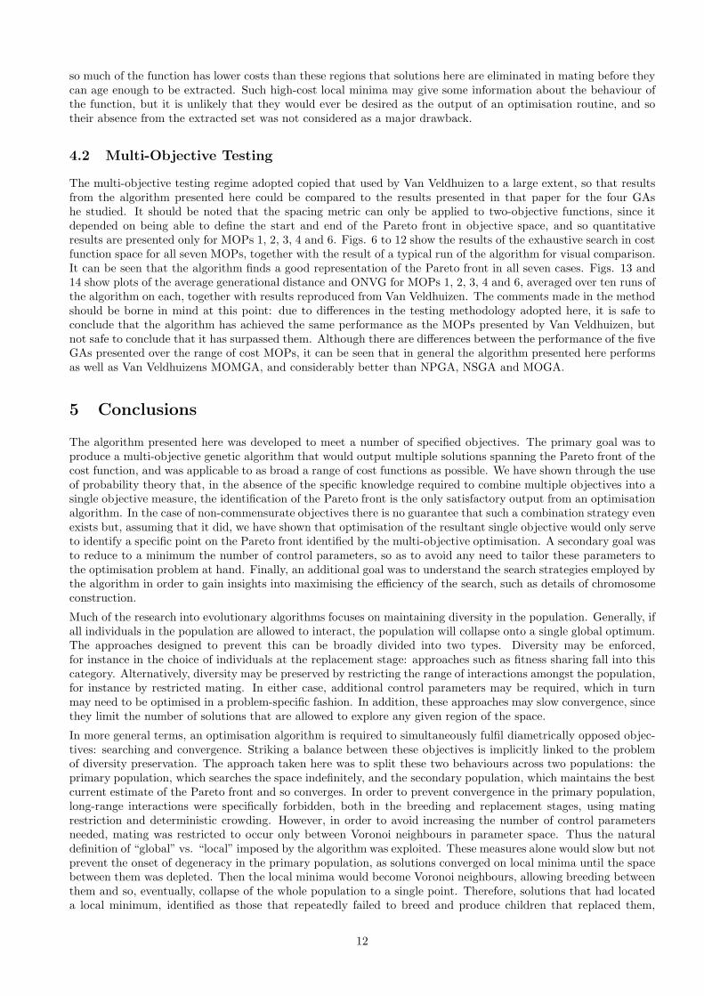
Since the algorithm presented here was designed to solve a multi-objective optimisation problem, the diagnosis ofdementing diseases problem described above, no great effort was made to test its performance on single objectiveoptimisation problems. In fact, only one problem was implemented, the six-hump camelback function [4]

f(x1, x2) = (4 − 2.1x21 +

x41

3)x2

1 + x1x2 + (−4 + 4x22)x

22 where − 3 < x1 < 3 and − 2 < x2 < −2 (3)

The function, shown in Fig. 2 has six local optima, of which two are global. Two more are local with relativelylow costs (compared to the range of values exhibited by the function between the spatial limits imposed), and thelast two are local with relatively high costs.

x1 x2 f(x1, x2)0.08984201310 -0.7126564030 -1.031628

-0.088984201310 0.7126564030 -1.0316281.703606715 -0.796083568 -0.215464-1.703606715 0.796083568 -0.215464-1.607104753 -0.568651454 2.1042501.607104753 0.568651454 2.104250

Table 1: Optima of the six-hump camelback function.

This function was used during the coding to test convergence before the features specific to multiple objectives(specialisation of patricide with the direction vectors, and the alterations to the extraction management function)were incorporated. It also served to illustrate some aspects of the behaviour of the algorithm. However, no testsof the rate of convergence were performed, as the GA cannot compete with other optimisation routines on such asimple function: a crude hill-climber can find the optima in a few tens of evaluations of the cost function, whereasthe GA may require this many to set up the initial population, before any convergence is even attempted.

3.2 Multi-objective Testing

A number of real-valued test problems are described in the literature, and a suite of the most popular suchfunctions have been collected in [24]. The same author has tested a number of multi-objective genetic algorithmswith these test functions, using a number of performance metrics [26]. In addition, many other authors e.g.[21] use subsets of these functions to test a range of algorithms. For ease of comparison to previously publishedalgorithms, the algorithm presented here was tested on the same functions. The test functions are given in Table2. Although the no free lunch theorems imply that no guarantee can be given for the general performance ofa multi-objective genetic algorithm, and therefore no amount of testing can predict its performance on somepreviously un-encountered function, testing on functions that exhibit a broad range of characteristics can at leastindicate whether an algorithm is likely to perform well on some new function exhibiting a mixture of the samecharacteristics, and this test suite was chosen to give as broad a range of cost function behaviours as possible.

Van Veldhuizen [24] has collected together a suite of real-valued test functions, and tested a number of algorithmswith a number of performance metrics [26]. For ease of comparison to previously published algorithms, thealgorithm presented here was tested in the same way. The test functions are given in Table 2. This test suite waschosen to give as broad a range of cost function behaviours as possible.

9

MOP Definition ConstraintsMOP1:Ptrue connected,PFtrue convex

F = (f1(x), f2(x)) where

f1(x) = x2,f2(x) = (x − 2)2

−105 ≤ x ≤ 105

MOP2:Ptrue connected,PFtrue concave,number of decisionvectors scalable

F = (f1(x, f2(x)) where

f1(x) = 1 − exp(−∑n

i=1(xi − 1√n)2),

f2(x) = 1 − exp(−∑n

i=1(xi + 1√n)2)

−4 ≤ xi ≤ 4; i = 1, 2, 3

MOP3:Ptrue disconnected,PFtrue discon-nected, 2 Paretocurves

F = −(f1(x, y), f2(x, y)) where

f1(x, y) = −[1 + (A1 −B1)2 + (A2 −B2)

2],f2(x, y) = −[(x + 3)2 + (y + q)2]

−3.1416 ≤ x, y ≤ 3.1416,A1 = 0.5 sin 1−2 cos1+sin 2−1.5 cos2,A2 = 1.5 sin 1−cos 1+2 sin2−0.5 cos2,B1 = 0.5 sinx−2 cosx+sin y−1.5 cos y,B2 = 1.5 sinx−cosx+2 sin y−0.5 cos y,

MOP4:Ptrue disconnected,PFtrue discon-nected, 3 Paretocurves, number ofdecision vectorsscalable

F = (f1(x), f2(x)) where

f1(x) =∑n−1

i=1 (−10e(−0.2)√

x21+x2

i+1)f2(x) =

∑n

i=1(|xi|0.8 + 5 sin(xi)3)

−5 ≤ xi ≤ 5; i = 1, 2, 3

MOP5:Ptrue disconnectedand un-symmetric,PFtrue connected,a 3D Pareto curve

F = (f1(x, y), f2(x, y), f3(x, y)) where

f1(x, y) = 0.5(x2 + y2) + sin(x2 + y2)

f2(x, y) = (3x−2y+4)2

8 + (x−y+1)2

27 + 15

f3(x, y) = 1(x2+y2+1) − 1.1e(−x2−y2)

−3 ≤ x, y ≤ 3

MOP6:Ptrue disconnected,PFtrue discon-nected, 4 Paretocurves, numberof Pareto curvesscalable

F = (f1(x, y), f2(x, y)) where

f1(x, y) = x

f2(x, y) =(1 + 10y)[1 − ( x

1+10y)α − x

1+10ysin(2πqx)]

0 ≤ x, y ≤ 1,

q = 4,α = 2

MOP7:Ptrue connected,PFtrue discon-nected

F = (f1(x, y), f2(x, y), f3(x, y)) where

f1(x, y) = (x−2)2

2 + (y+1)2

13 + 3

f2(x, y) = (x+y−3)2

36 + (−x+y+2)2

8 − 17

f3(x, y) = (x+2y−1)2

175 + (2y−x)2

17 − 13

−40 ≤ x, y ≤ 400

Table 2: Multi-objective test functions

Four test metrics are suggested. The first is generational distance,

G =(∑n

i=1 dpi )

1p

n(4)

which describes how far in objective space the Pareto front PFknown produced by the optimisation algorithm isfrom the true Pareto front PFtrue, where n is the number of vectors in PFknown, p = 2 and di is the Euclideandistance in objective space between each vector and the nearest member of PFtrue. The second is spacing,

S =

√

√

√

√

1

1 − n

n∑

i+1

(dmean − di)2 (5)

which quantifies how evenly spread the members of PFknown are along the Pareto front. The third is overallnon-dominated vector generation, ONVG

ONV G = |PFknown| (6)

10

the number of solutions in PFknown, and the fourth is overall non-dominated vector generation ratio,

ONV GR =|PFknown||PFtrue|

(7)

the ration of the number of solutions in PFknown to the number in PFtrue at some specified resolution of the space.

Van Veldhuizen compares four multi-objective genetic algorithms: the multi-objective genetic algorithm (MOGA),MOMOGA, the niched Pareto genetic algorithm (NPGA) and non-dominated sorting genetic algorithm (NSGA).The testing procedure requires prior knowledge of the true Pareto front, which can be obtained by exhaustivesearching of the space at some resolution for simple MOPs such as the test functions described, although obviouslythis is not practical for MOPs of any significant difficulty. Van Veldhuizen implements a binary-valued algorithmand defines the computational grid used in both the exhaustive search and the MOGAs such that 224 points inthe space are tested. No solution cost specific termination criterion for the algorithms is implemented: instead thesearch is terminated when the number of cost function evaluations exceeds 216, such that 0.39% of the space issearched. The exhaustive search is implemented on a high powered parallel architecture. The MOGAs are eachrun ten times on each MOP, and averages calculated for the four test metrics described above.

Due to lack of available processor time, the same test procedure could not be implemented for the algorithmdescribed here. The exhaustive search was performed at a resolution of 0.001 on all coordinates of the MOPs,resulting in a considerably coarser representation of the space than Van Veldhuizen used. However, the algorithmitself does not restrict solutions to lie on a grid, and so in theory an infinite number of points in the space areavailable for investigation. Since the algorithm uses a computational resolution finer than the exhaustive search,a minimum bound exists on the generational distance for each MOP, and the test procedure therefore provides alower limit estimate of the performance of the algorithm. This limits the conclusions that can be drawn from theresults: it is possible to say that the algorithm has failed to find the true Pareto front to the accuracy used inthe exhaustive search within the number of cost function evaluations imposed, but not that it has improved uponit, or upon the results demonstrated by Van Veldhuizen. Nevertheless, this remains sufficient to demonstrate thefeasibility and promise of the algorithm.

Although the generation distance and ONVG provide a good indication of the knowledge of the Pareto frontgenerated by the algorithm, the spacing and ONVGR may be less useful. These relate to the requirement forequal spacing of the solutions along the Pareto front, and each of the four algorithms tested by Van Veldhuizenincorporates fitness sharing in an attempt to enforce even spacing of the solutions. For the reasons outlined above,the algorithm presented here uses no such mechanism. The spatial accuracy variable used to filter the extractedset was set to 0.00001 for all MOPs, a level at which it was found to have no significant effect.

4 Results

4.1 Single-Objective Testing

In order to demonstrate that the inclusion of the Voronoi mating restriction enabled the algorithm to preservediversity in the general population indefinitely, it was tested on the six-hump camelback function, with a popu-lation size of 100, an extraction age of 5, and the default mutation probabilities of, using both random selectionof individuals for mating, and Voronoi restricted mating. The spatial positions of the solutions in the generalpopulation at each generation for the first 25 generations for both cases are shown in Figs. 3 and 4 respectively.Clearly in the first case both global optima are found, but one global optimum is eliminated from the populationafter around 15 generations and never recovered. The population collapses onto one of the global optima (whichone is random), such that the majority of the individuals in the population are at exactly the same point in thespace. Random immigrants are therefore quickly eliminated from the population during breeding with these highlyfit individuals, such that further searching of the space is prevented.

In the second case, diversity is preserved and both global optima (and two of the local optima) persist in thegeneral population. Whilst the search is focused in the region of the global optima, such that detailed explorationof these regions can be performed, individuals in these regions cannot breed with random immigrants in distantregions of the space, and so searching of the space continues indefinitely.

Fig. 5 shows the positions of the members of the extracted set after 25 generations with the parameters describedabove, plotted on a 2D contour plot of the function. The two global minima are found and the two lower-costlocal minima are found to within machine precision within 25 generations, all four being captured in a single run.The extracted set never contained more than four entries, due to the check implemented to ensure that multiplesolutions in the same local minium were discarded. The remaining two, high-cost local minima are not found, as

11

so much of the function has lower costs than these regions that solutions here are eliminated in mating before theycan age enough to be extracted. Such high-cost local minima may give some information about the behaviour ofthe function, but it is unlikely that they would ever be desired as the output of an optimisation routine, and sotheir absence from the extracted set was not considered as a major drawback.

4.2 Multi-Objective Testing

The multi-objective testing regime adopted copied that used by Van Veldhuizen to a large extent, so that resultsfrom the algorithm presented here could be compared to the results presented in that paper for the four GAshe studied. It should be noted that the spacing metric can only be applied to two-objective functions, since itdepended on being able to define the start and end of the Pareto front in objective space, and so quantitativeresults are presented only for MOPs 1, 2, 3, 4 and 6. Figs. 6 to 12 show the results of the exhaustive search in costfunction space for all seven MOPs, together with the result of a typical run of the algorithm for visual comparison.It can be seen that the algorithm finds a good representation of the Pareto front in all seven cases. Figs. 13 and14 show plots of the average generational distance and ONVG for MOPs 1, 2, 3, 4 and 6, averaged over ten runs ofthe algorithm on each, together with results reproduced from Van Veldhuizen. The comments made in the methodshould be borne in mind at this point: due to differences in the testing methodology adopted here, it is safe toconclude that the algorithm has achieved the same performance as the MOPs presented by Van Veldhuizen, butnot safe to conclude that it has surpassed them. Although there are differences between the performance of the fiveGAs presented over the range of cost MOPs, it can be seen that in general the algorithm presented here performsas well as Van Veldhuizens MOMGA, and considerably better than NPGA, NSGA and MOGA.

5 Conclusions

The algorithm presented here was developed to meet a number of specified objectives. The primary goal was toproduce a multi-objective genetic algorithm that would output multiple solutions spanning the Pareto front of thecost function, and was applicable to as broad a range of cost functions as possible. We have shown through the useof probability theory that, in the absence of the specific knowledge required to combine multiple objectives into asingle objective measure, the identification of the Pareto front is the only satisfactory output from an optimisationalgorithm. In the case of non-commensurate objectives there is no guarantee that such a combination strategy evenexists but, assuming that it did, we have shown that optimisation of the resultant single objective would only serveto identify a specific point on the Pareto front identified by the multi-objective optimisation. A secondary goal wasto reduce to a minimum the number of control parameters, so as to avoid any need to tailor these parameters tothe optimisation problem at hand. Finally, an additional goal was to understand the search strategies employed bythe algorithm in order to gain insights into maximising the efficiency of the search, such as details of chromosomeconstruction.

Much of the research into evolutionary algorithms focuses on maintaining diversity in the population. Generally, ifall individuals in the population are allowed to interact, the population will collapse onto a single global optimum.The approaches designed to prevent this can be broadly divided into two types. Diversity may be enforced,for instance in the choice of individuals at the replacement stage: approaches such as fitness sharing fall into thiscategory. Alternatively, diversity may be preserved by restricting the range of interactions amongst the population,for instance by restricted mating. In either case, additional control parameters may be required, which in turnmay need to be optimised in a problem-specific fashion. In addition, these approaches may slow convergence, sincethey limit the number of solutions that are allowed to explore any given region of the space.

In more general terms, an optimisation algorithm is required to simultaneously fulfil diametrically opposed objec-tives: searching and convergence. Striking a balance between these objectives is implicitly linked to the problemof diversity preservation. The approach taken here was to split these two behaviours across two populations: theprimary population, which searches the space indefinitely, and the secondary population, which maintains the bestcurrent estimate of the Pareto front and so converges. In order to prevent convergence in the primary population,long-range interactions were specifically forbidden, both in the breeding and replacement stages, using matingrestriction and deterministic crowding. However, in order to avoid increasing the number of control parametersneeded, mating was restricted to occur only between Voronoi neighbours in parameter space. Thus the naturaldefinition of “global” vs. “local” imposed by the algorithm was exploited. These measures alone would slow but notprevent the onset of degeneracy in the primary population, as solutions converged on local minima until the spacebetween them was depleted. Then the local minima would become Voronoi neighbours, allowing breeding betweenthem and so, eventually, collapse of the whole population to a single point. Therefore, solutions that had locateda local minimum, identified as those that repeatedly failed to breed and produce children that replaced them,

12

were extracted to the second population and replaced with random immigrants. This prevented optimal solutionsfrom dominating the population, and introduced enough randomness that searching continued indefinitely withoutlimiting the search behaviour of the individual solutions. The use of extraction/random immigration also conferreda second benefit, in that it eliminated population size as a control parameter, allowing the algorithm to exploit aninfinite population over infinite time. To further eliminate control parameters, the parameters controlling randomaspects of the algorithm, such as mutation probabilities, were also placed under the control of the algorithm asfurther objectives to be optimised.

The algorithm has been tested on a number of real-valued test problems for the test suite collated by Van Veld-huizen, allowing comparison with the four algorithms he tested. In general, over the range of test problems andon the three metrics he used (generational distance, spacing, and ONVG), the algorithm at least competes withMOMGA, and is superior to NPGA, NSGA and MOGA. We therefore conclude that, in addition to the advantagesoutlined above, the algorithm performs at least as well as the state-of-the-art on these simple test problems. How-ever, it should be noted that all of these simple test problems share a common flaw. A GA has two search operatorsavailable: random mutation and crossover. Random mutation allows the algorithm to hill climb, but in theorycrossover allows much more rapid convergence by forming solutions from building blocks: optimised sub-sectionsof the genome. Indeed, if the building blocks strategy is not available as a search strategy, there seems little pointin using a GA, as no improvements can be made over the performance of other hill climbing algorithms. Therefore,we are forced to ask what kind of problems are amenable to solution in this building block fashion, and how toconstruct chromosome representations of solutions to these problems that allow the strategy to be applied.

In order that a problem can be solved by the building blocks strategy, it must be possible to optimise sub-sectionsof the genome independent of the rest of the genome, and combine such sub-sections to form fitter genomes. Thedefinition of independence requires careful treatment, as there are several possible forms of independence. Givena single objective ai, a function of a set of n parameters ci, portions of the genome are independent if the costfunction can be expressed as a sum over these portions

ai = f(c) =∑

cp,q

f(cp,q) (8)

where the parameters cp,q are some subset (p to q)of the parameters c1−n and the sum is performed over all suchsubsets. These parameter subsets are commonly referred to in the GA literature as schemata, and “building blocks”are commonly defined as highly fit, low-order, short-length schemata. Schemata correspond to hyperplanes in thesearch space.

Given that the ability to combine building blocks is a prerequisite of efficient GA use, some conclusions can bedrawn concerning the problems to which GAs can be efficiently applied. Clearly, the simple test problems used inthis paper, and more generally in the GA literature, do not possess this property and so are not effective tests ofGA efficiency, beyond indicating the ability to hill-climb. More realistic test problems would include the TravellingSalesman Problem [13]. This involves planning the shortest path that visits a set of cities exactly once and returnsto the starting point. Depending on the geographical layout of the cities, it may be possible to optimise smallportions of the path independent of the remainder of the cities. The brain atrophy analysis described in theintroduction also possesses this property: each pair of points defines a decision boundary in the brain, and it maybe possible to optimise a single decision boundary (possibly by matching its position to some physical structure,such as a boundary between lobes) independent of the remaining boundaries. Note that this does not imply thatthe problem can be solved by applying optimisation techniques to each portion of the genome in turn. Portions ofthe genome may still be weakly coupled: in the brain atrophy analysis, the points at which the decision boundariesintersect will be governed by more than two points. In addition, the most efficient division of the genome intoschemata may not be available, and the GA can explore multiple possibilities.

We can now draw some conclusions on the types of problems that GAs can solve, the search strategies they canuse, and how to most efficiently construct a genome. Firstly, in order for recombination to act efficiently, theproblem must be solvable by the combination of building blocks. This requires at least partial independence ofschemata within the genome, and in turn dictates how the genome should be constructed (and how the crossoveroperator should be designed). Optimisation of such schemata implies detection of a highly fit hyperplane within thesearch space, representing optimisation of a sub-set of parameters. Combination of such schemata then representsdetection of the crossover points of the hyperplanes to detect global optima.

It has been stated in the past that the combination of mating restriction and deterministic crowding, as used in thealgorithm presented here, would prevent certain types of recombination events from occurring [14]. Specifically,in a deceptive and massively where the only feasible way to locate the deceptive global peak was by combinationof schemata from the local optima, and furthermore there were less fit regions between the local and global

13

optima, the presence of solutions in these less fit regions would prohibit the desired recombination events viathe mating restriction. However, the arguments outlined above demonstrate that such problems are somewhatartificial. If the problem is amenable to GA optimisation and the genome is constructed efficiently, the searchspace will contain local optimal hyperplanes that intersect at global optimal points. The GA will then hill climbor randomly search on schemata to find the hyperplanes, and follow them to detect the global optima. In thatcase, if the definition of Voronoi neighbours is selected with care, mating will occur between the solutions climbingalong different hyperplanes that are closest to the intersection points, and thus the intersection points will belocated by recombination. We conclude that the combination of mating restriction with deterministic crowdingwould not hinder the convergence to global optima on realistic multi-objective functions where the objectives wereindependent. This is an issue that can be addressed in chromosome construction and objective definition, if onlyto enhance the possibility of creating building blocks, and therefore the problems typified by deceptive functionsshould not have undue influence on the design of algorithms. However, it is recognised that additional testing onrealistic test problems, such as the Travelling Salesman Problem, will be required to elucidate this point.

References

[1] T Back. Optimal mutation rates in genetic search. In S Forrest, editor, Proceedings of the Fifth InternationalConference on Genetic Algorithms, pages 2–8. Morgan Kaufmann Publishers, 1993.

[2] P A Bromiley, N A Thacker, and P Courtney. Colour image segmentation by non-parametric density estimationin colour space. In T Cootes and C Taylor, editors, Proceedings of the British Machine Vision Conference,pages 283–292. British Machine Vision Association, 2001.

[3] C A C Coello. List of references on evolutionary multiobjective optimisation, 1999. Available at:http://www.lania.mx/EMOO.

[4] L C W Dixon and G P Szego. Towards Global Optimisation 2. North Holland, Amsterdam, 1978.

[5] L Davis (Ed.). Handbook of Genetic Algorithms. Van Nostrand Reinhold, New York, 1991.

[6] C M Fonseca and P J Fleming. An overview of evolutionary algorithms in multiobjective optimization.Evolutionary Computation, 3(1):1–16, 1995.

[7] M P Fourman. Compaction of symbolic layout using genetic algorithms. In J J Grefensette, editor, Proceedingsof the First International Conference on Genetic Algorithms and their Applications, pages 141–153, Pittsburg,PA, July 1985. Lawrence Erlbaum Associates, Publishers, Hillsdale, New Jersey.

[8] D E Goldberg. Genetic Algorithms in Search, Optimization and Machine Learning. Addison-Wesley, Reading,MA, 1989.

[9] D E Goldberg, K Deb, and J H Clark. Genetic algorithms, noise, and the sizing of populations. TechnicalReport IlliGAL Report No. 91090, Illinois Genetic Algorithms Laboratory, http://www-illigal.ge.uiuc.edu,191.

[10] D E Goldberg, K Deb, and J H Clark. Genetic algorithms, noise, and the sizing of populations. ComplexSystems, 6:333–362, 1992.

[11] D E Goldberg and J Richardson. Genetic algorithms with sharing for multimodal function optimisation. InJ J Grefensette, editor, Genetic Algorithms and their Applications: Proceedings of the Second InternationalConference on Genetic Algorithms, pages 41–49. Lawrence Erlbaum Associates, Publishers, Hillsdale, NewJersey., 1987.

[12] S P Larcombe. Implementing Heterogeneous Systems in a Three-Dimensional Packaging Technology. PhDthesis, Department of Electronic and Electrical Engineering, University of Sheffield, 1996.

[13] P Larranaga, C M H Kuijpers, R H Murga, I Inza, and S Dizdarevic. Genetic algorithms for the travellingsalesman problem: A review of representations and operators. Artificial Intelligence Review, 13:129–170, 1999.

[14] S W Mahfoud. Niching Methods for Genetic Algorithms. PhD thesis, Illinois Genetic Algorithms Laboratory,Department of General Engineering, University of Illinois at Urbana-Champaign, 1995.

14

[15] I Ono, H Kita, and S Kobayashi. A robust real-coded genetic algorithm using unimodal normal distributioncrossover augmented by uniform crossover: Effects of self-adaptation of crossover probabilities. In W Banzhaf,J Daida, A E Eiben, M H Garzon, V Honavar, M Jakiela, and R E Smith, editors, Proceedings of the Geneticand Evolutionary Computation Conference (GECCO-99), pages 496–503. Morgan Kaufmann Publishers, 1999.

[16] W H Press, S A Teukolosky, W T Vetterling, and B P Flannery. Numerical Recipes in C: The Art of ScientificComputing (Second Edition). Cambridge University Press, Cambridge, U.K., 1992.

[17] H H Rosenbrock. An automatic method for finding the greatest or least value of a function. Comput. J.,3:175–184, 1960.

[18] J D Schaffer. Multiple objective optimisation with vector evaluated genetic algorithms. In J J Grefensette,editor, Proceedings of the First International Conference on Genetic Algorithms and their Applications, pages93–100, Pittsburg, PA, July 1985. Lawrence Erlbaum Associates, Publishers, Hillsdale, New Jersey.

[19] J R Schott. Fault tolerant design using single and multicriteria genetic algorithm optimisation. Master’sthesis, Department of Aeronautics and Astronautics, Massachusetts Institute of Technology, Cambridge, Mas-sachusetts, 1995.

[20] N Srinivas and K Deb. Multiobjective optimisation using nondominated sortinfg in genetic algorithms. Evo-lutionary Computation, 2(3):221–284, 1994.

[21] K C Tan, T H Lee, and E F Khor. Evolutionary algorithms with dynamic population size and local explorationfor multiobjective optimisation. IEEE Transactions on Evolutionary Computation, 5(6):565–588, 2001.

[22] N A Thacker, A J Lacey, P Courtney, and G S Rees. An empirical design methodology for the construction ofmachine vision systems. Technical Report TINA Memo No. 2002-005, Neuroimage Analysis Center (NiAC),http://www.tina-vision.net, 2002.

[23] N A Thacker, A R Varma, D Bathgate, J S Snowden, D Neary, and A Jackson. Quantification of thedistribution of cerebral atrophy in dementing diseases. In Proceeding MIUA, pages 61–64, London, July 2000.BMVA.

[24] D A Van Veldhuizen. Multiobjective Evolutionary Algorithms: Classifications, Analyses and New Innovations.PhD thesis, Graduate School of Engineering, Air Force Institute of Technology, 1999.

[25] D A Van Veldhuizen and G B Lamont. Multi-objective evolutionary algorithm research: A history andanalysis. Technical Report Technical Report TR-98-03, Air Force Institute of Technology, Wright-PattersonAir Force Base, OH 45433-7765, 1998.

[26] D A Van Veldhuizen and G B Lamont. On measuring multiobjective evolutionary algorithm performance. InProceedings of the 2000 Congress on Evolutionary Computation, pages 204–211, 2000.

[27] G Voronoi. Recherches sur les paralleloedres primitives. J. reine angew. Math., 134:198–287, 1908.

[28] D H Wolpert and L Thiele. No free lunch theorems for optimisation. IEEE Transactions on EvolutionaryComputation, 1(1):67–82, 1997.

15

6 Figures

Figure 1: The derivation of the Voronoi cell crossing constraint for mating restriction. The solid points are knotpoints and the dashed lines are the cell boundaries. The darker line is the boundary crossed by the allowed stepAC. The constraint tests that the intersection I of this plane with the step AB is at less than half the length ofAB, to the mid-point M.

-2-1 0 1 2 3 4 5 6 4

3 2.2 2.1 2

1.5 1

0.5 0

-0.5 -1

-1.5 -1 -0.5 0 0.5 1 1.5-1

-0.5

0

0.5

1

-2-1 0 1 2 3 4 5 6

Figure 2: The six-hump camelback function.

16

’junk_5’

0 5

10 15

20 25 -3 -2 -1 0 1 2 3

-2

-1.5

-1

-0.5

0

0.5

1

1.5

2

Figure 3: The general population during the first 25 generations of optimisation on the six hump camelbackfunction, for a population size of 100 and extraction age of 5, with random selection for breeding.

’junk_5_voronoid’

0 5

10 15

20 25 -2 -1.5 -1 -0.5 0 0.5 1 1.5 2

-2

-1.5

-1

-0.5

0

0.5

1

1.5

2

Figure 4: The general population during the first 25 generations of optimisation on the six hump camelbackfunction, for a population size of 100 and extraction age of 5, with Voronoi selection for breeding.

17

-1

-0.5

0

0.5

1

-1.5 -1 -0.5 0 0.5 1 1.5

’shcf_es’’shcf_contours’

Figure 5: 2D projection of the six-hump camelback function, showing the extracted set solutions found by the GAafter 25 generations with a population of 100, extraction age of 5, and default mutation probabilities. Note thatthe 2 high-cost local optima are not entered into the extracted set.

0

0.5

1

1.5

2

2.5

3

3.5

4

0 0.5 1 1.5 2 2.5 3 3.5 4

’iter32000_pop100_ext5_acc01_noav_mop1_8_costs’

(a)

0

0.5

1

1.5

2

2.5

3

3.5

4

4.5

0 0.5 1 1.5 2 2.5 3 3.5 4

’exhaust_mop1_costs’

(b)

Figure 6: Sample output from algorithm (a) and exhaustive search results (b) for MOP1.

0

0.1

0.2

0.3

0.4

0.5

0.6

0.7

0.8

0.9

1

0 0.1 0.2 0.3 0.4 0.5 0.6 0.7 0.8 0.9 1

’iter32000_pop100_ext5_acc01_noav_mop2_8_costs’

(a)

0

0.1

0.2

0.3

0.4

0.5

0.6

0.7

0.8

0.9

1

0 0.1 0.2 0.3 0.4 0.5 0.6 0.7 0.8 0.9 1

’exhaust_mop2_costs’

(b)

Figure 7: Sample output from algorithm (a) and exhaustive search results (b) for MOP2.

18

0

5

10

15

20

25

30

0 2 4 6 8 10 12 14 16 18

’iter32000_pop100_ext5_acc01_noav_mop3_5_costs’

(a)

0

5

10

15

20

25

0 2 4 6 8 10 12 14 16 18

’exhaust_mop3_costs’

(b)

Figure 8: Sample output from algorithm (a) and exhaustive search results (b) for MOP3.

-12

-10

-8

-6

-4

-2

0

2

-20 -19 -18 -17 -16 -15 -14 -13 -12

’iter32000_pop100_ext5_acc01_noav_mop4_9_costs’

(a)

-12

-10

-8

-6

-4

-2

0

2

-20 -19 -18 -17 -16 -15 -14 -13

’exhaust_mop4_costs’

(b)

Figure 9: Sample output from algorithm (a) and exhaustive search results (b) for MOP4.

’iter32000_pop100_ext5_acc01_noav_mop5_8_costs’

0 1

2 3

4 5

6 7

8 9

15

15.5

16

16.5

17

17.5

-0.1

-0.05

0

0.05

0.1

0.15

0.2

(a)

’exhaust_mop5_costs’

0 1

2 3

4 5

6 7

8 9

15 15.5

16 16.5

17 17.5

-0.1

-0.05

0

0.05

0.1

0.15

0.2

(b)

Figure 10: Sample output from algorithm (a) and exhaustive search results (b) for MOP5.

19

-0.6

-0.4

-0.2

0

0.2

0.4

0.6

0.8

1

1.2

0 0.1 0.2 0.3 0.4 0.5 0.6 0.7 0.8 0.9

’iter32000_pop100_ext5_acc01_noav_mop6_5_costs’

(a)

-0.6

-0.4

-0.2

0

0.2

0.4

0.6

0.8

1

0 0.1 0.2 0.3 0.4 0.5 0.6 0.7 0.8 0.9

’exhaust_mop6_costs’

(b)

Figure 11: Sample output from algorithm (a) and exhaustive search results (b) for MOP6.

’mop7_test’

3 3.2

3.4 3.6

3.8 4

4.2 4.4

-17-16.9

-16.8-16.7

-16.6-16.5

-16.4

-13-12.9-12.8-12.7-12.6-12.5-12.4-12.3-12.2-12.1

-12

(a)

’mop7_test_exhaust_2_costs’

2.8 3

3.2 3.4

3.6 3.8

4 4.2

-17 -16.95-16.9-16.85-16.8-16.75-16.7-16.65-16.6-16.55-16.5

-13-12.9-12.8-12.7-12.6-12.5-12.4-12.3-12.2-12.1

-12

(b)

Figure 12: Sample output from algorithm (a) and exhaustive search results (b) for MOP7.

(a)

0

0.05

0.1

0.15

0.2

0.25

0.3

0.35

0.4

0.45

0 1 2 3 4 5 6 7

Gen

erat

iona

l Dis

tanc

e

MOP

MOVNGA: MOP1-7

’iter32000_ext5_pop100_acc01_g’ using 1:2’iter32000_ext5_pop100_acc01_g’

(b)

Figure 13: Generational distance (lower is better) for the four MOEAs tested by Van Veldhuizen (a) and forMOVNGA (b).

20

(a)

0

50

100

150

200

250

300

350

400

0 1 2 3 4 5 6 7

ON

VG

MOP

MOVNGA: MOP1-7

’iter32000_ext5_pop100_acc01_onvg’ using 1:2’iter32000_ext5_pop100_acc01_onvg’

(b)

Figure 14: ONVG (higher is better) for the four MOEAs tested by Van Veldhuizen (a) and for MOVNGA (b).

21