Embed Size (px)
Citation preview
Multimedia Communications
Differential Coding
Copyright S. Shirani
Differential Coding • In many sources, the source output does not change a great
deal from one sample to the next. • This means that both the dynamic range and the variance of
the sequence of differences {dn=xn-xn-1} are significantly smaller than that of the source output sequence.
• For correlated sources the distribution of dn is highly peaked at zero.
• Techniques that transmit information by encoding differences are called differential encoding
Copyright S. Shirani
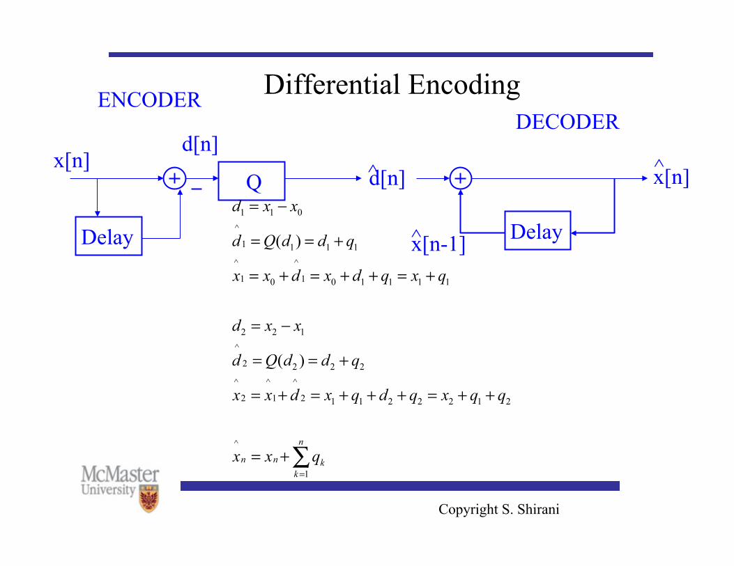
Differential Encoding
Delay Delay
Q x[n]
d[n] d[n] x[n]
x[n-1]
^ ^
ENCODER DECODER
^
Copyright S. Shirani
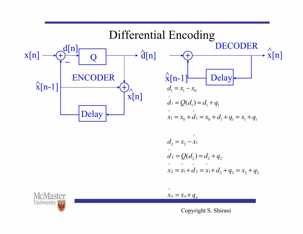
Differential Encoding
Delay
Delay
Q x[n] d[n]
d[n] x[n]
x[n-1] x[n-1]
x[n]
^ ^
^ ENCODER
DECODER
^ ^
Copyright S. Shirani
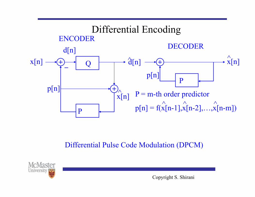
Differential Encoding
P
P
Q x[n] d[n]
d[n] x[n]
p[n]
p[n] x[n]
^ ^
^
ENCODER DECODER
P = m-th order predictor
p[n] = f(x[n-1],x[n-2],…,x[n-m]) ^ ^ ^
Differential Pulse Code Modulation (DPCM)
Copyright S. Shirani
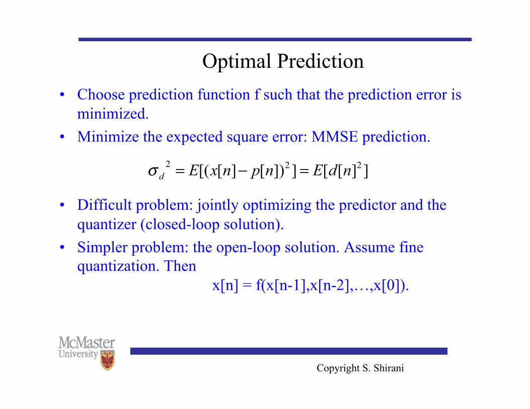
Optimal Prediction • Choose prediction function f such that the prediction error is
minimized. • Minimize the expected square error: MMSE prediction.
• Difficult problem: jointly optimizing the predictor and the quantizer (closed-loop solution).
• Simpler problem: the open-loop solution. Assume fine quantization. Then x[n] = f(x[n-1],x[n-2],…,x[0]).
~
Copyright S. Shirani
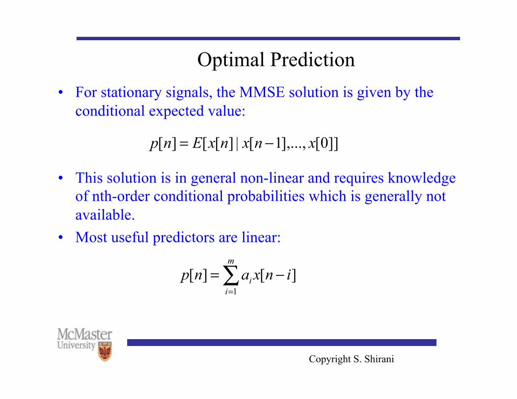
Optimal Prediction • For stationary signals, the MMSE solution is given by the
conditional expected value:
• This solution is in general non-linear and requires knowledge of nth-order conditional probabilities which is generally not available.
• Most useful predictors are linear:
Copyright S. Shirani
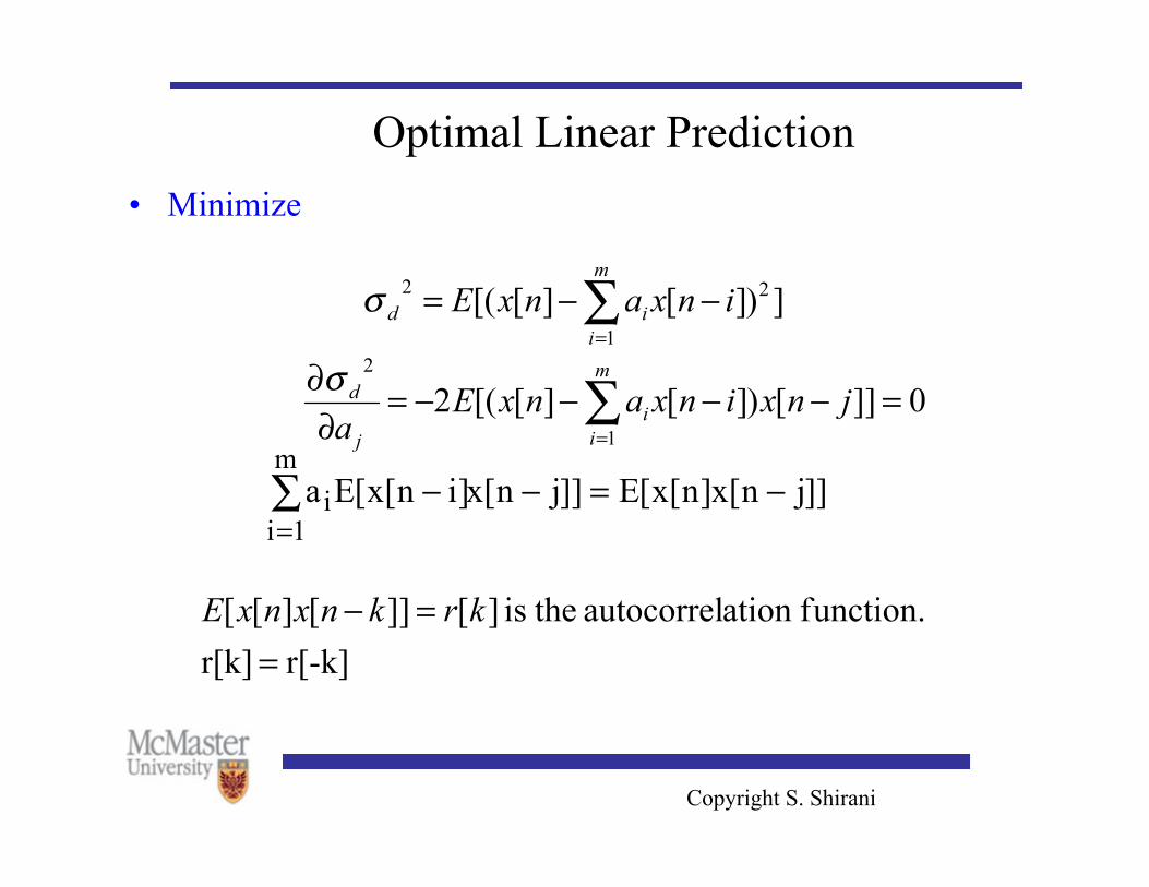
Optimal Linear Prediction • Minimize
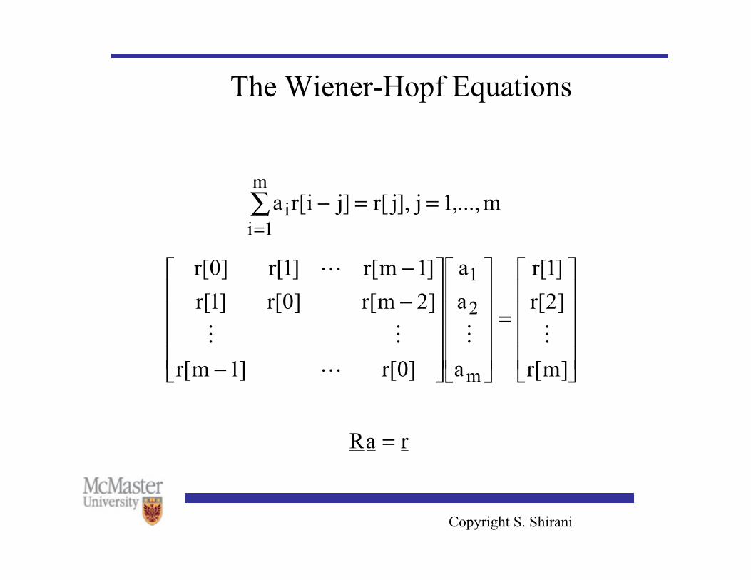
Copyright S. Shirani
The Wiener-Hopf Equations
Copyright S. Shirani
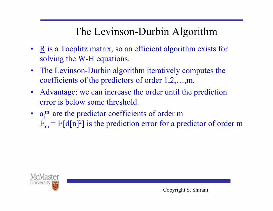
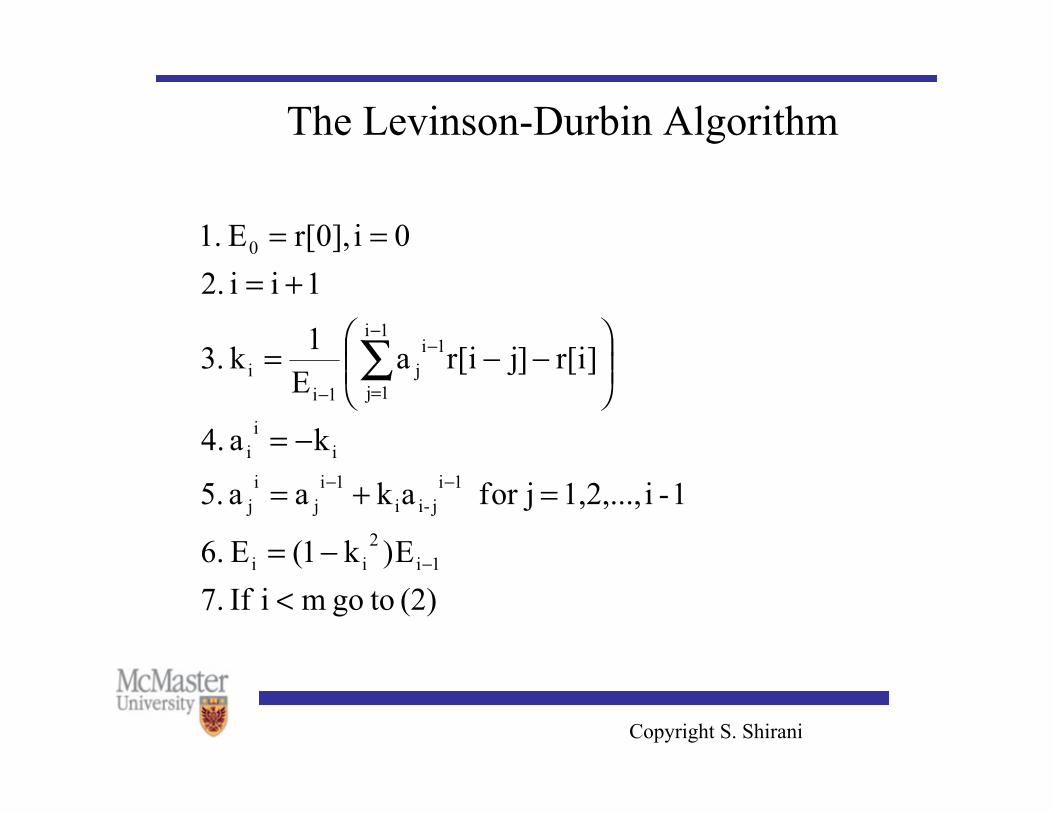
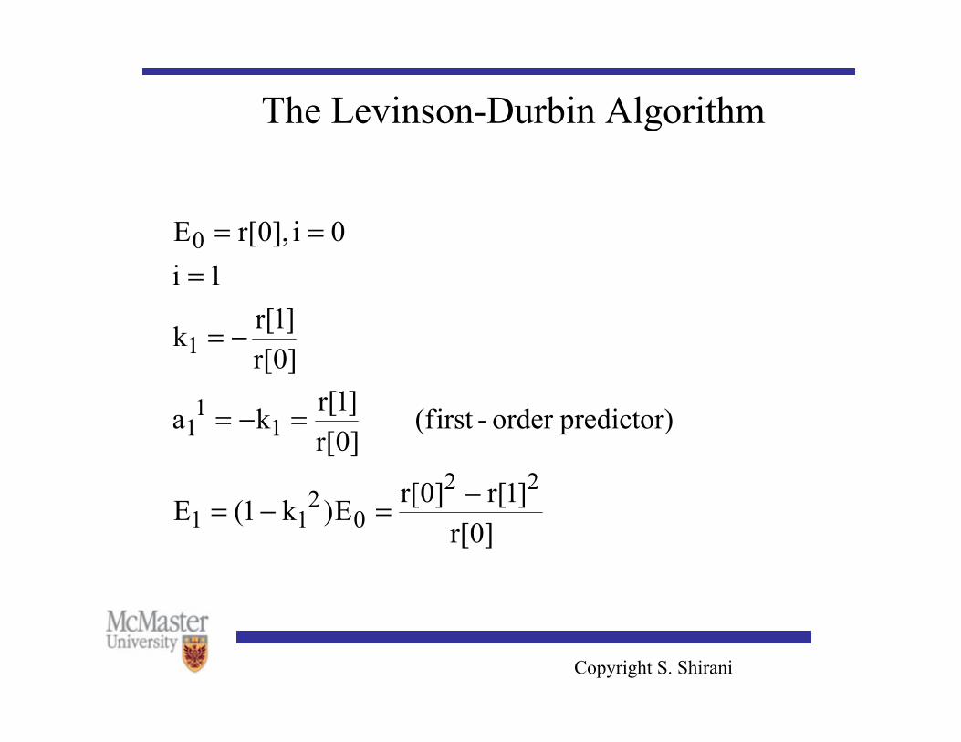
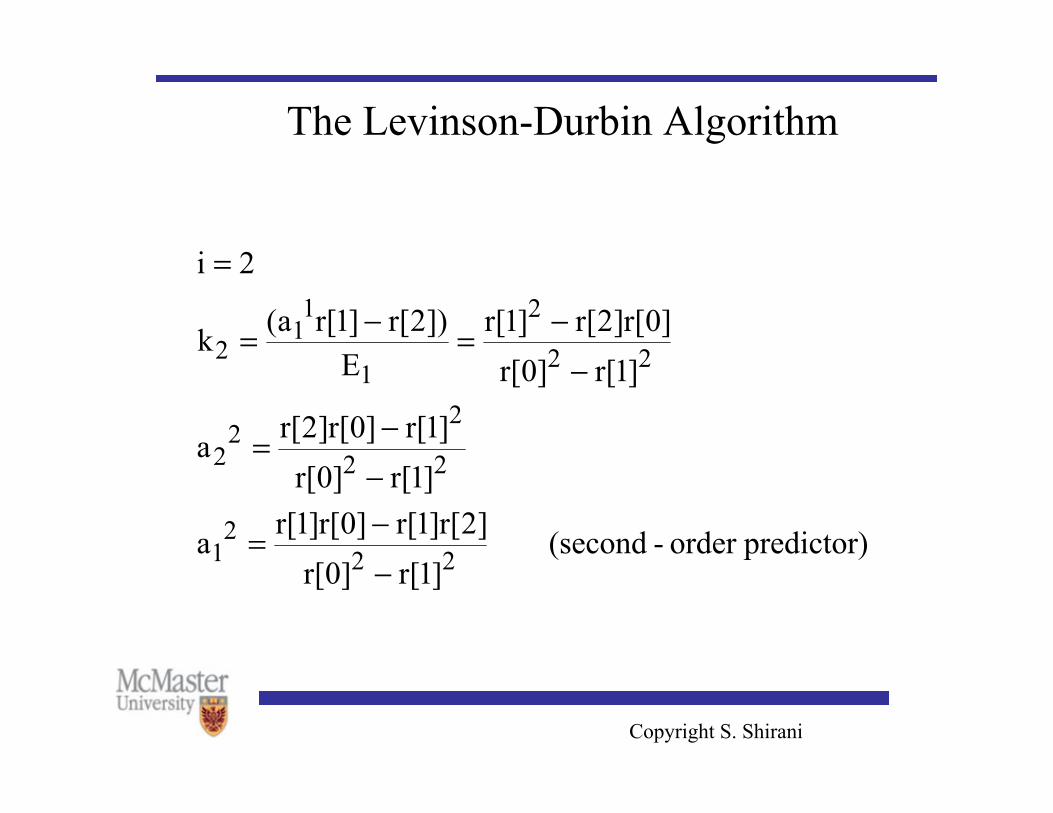
The Levinson-Durbin Algorithm • R is a Toeplitz matrix, so an efficient algorithm exists for
solving the W-H equations. • The Levinson-Durbin algorithm iteratively computes the
coefficients of the predictors of order 1,2,…,m. • Advantage: we can increase the order until the prediction
error is below some threshold. • aj
m are the predictor coefficients of order m Em = E[d[n]2] is the prediction error for a predictor of order m
Copyright S. Shirani
The Levinson-Durbin Algorithm
Copyright S. Shirani
The Levinson-Durbin Algorithm
Copyright S. Shirani
The Levinson-Durbin Algorithm
Copyright S. Shirani
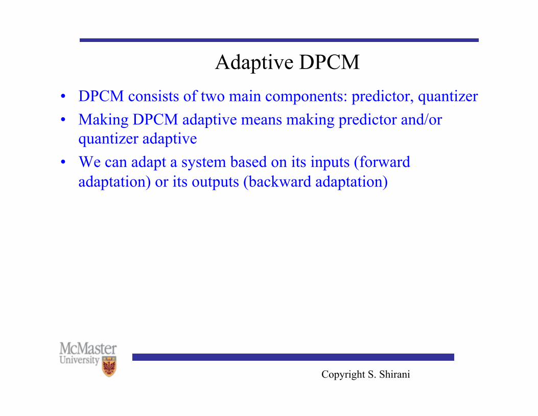
Adaptive DPCM • DPCM consists of two main components: predictor, quantizer • Making DPCM adaptive means making predictor and/or
quantizer adaptive • We can adapt a system based on its inputs (forward
adaptation) or its outputs (backward adaptation)
Copyright S. Shirani
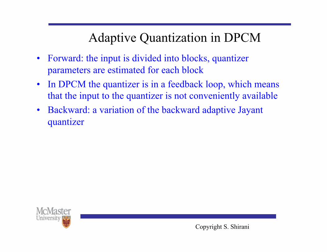
Adaptive Quantization in DPCM • Forward: the input is divided into blocks, quantizer
parameters are estimated for each block • In DPCM the quantizer is in a feedback loop, which means
that the input to the quantizer is not conveniently available • Backward: a variation of the backward adaptive Jayant
quantizer
Copyright S. Shirani
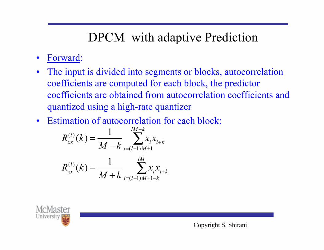
DPCM with adaptive Prediction • Forward: • The input is divided into segments or blocks, autocorrelation
coefficients are computed for each block, the predictor coefficients are obtained from autocorrelation coefficients and quantized using a high-rate quantizer
• Estimation of autocorrelation for each block:
Copyright S. Shirani
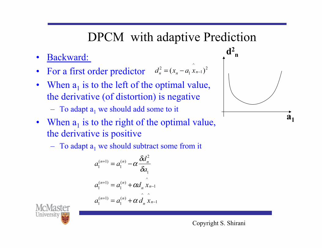
DPCM with adaptive Prediction • Backward: • For a first order predictor • When a1 is to the left of the optimal value,
the derivative (of distortion) is negative – To adapt a1 we should add some to it
• When a1 is to the right of the optimal value, the derivative is positive – To adapt a1 we should subtract some from it
d2n
a1
Copyright S. Shirani
DPCM with adaptive Prediction
Copyright S. Shirani
Delta modulator • Delta modulator: a very simple DPCM system with a 1-bit (2
level) quantizer • We can only represent sample to sample difference of Δ. • Substantial distortion if sample to sample difference is very
different from Δ. • Solution: sample the signal at a very high rate (several times
of the Nyquist rate)
Copyright S. Shirani
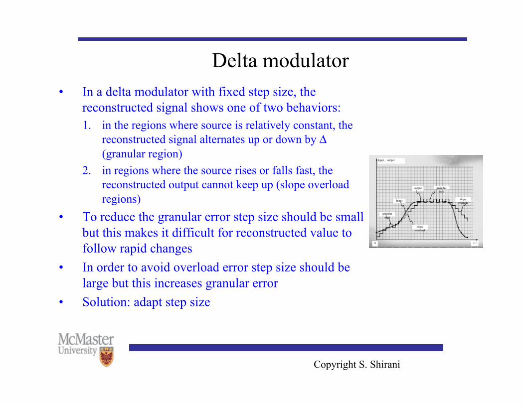
Delta modulator • In a delta modulator with fixed step size, the
reconstructed signal shows one of two behaviors: 1. in the regions where source is relatively constant, the
reconstructed signal alternates up or down by Δ (granular region)
2. in regions where the source rises or falls fast, the reconstructed output cannot keep up (slope overload regions)
• To reduce the granular error step size should be small but this makes it difficult for reconstructed value to follow rapid changes
• In order to avoid overload error step size should be large but this increases granular error
• Solution: adapt step size
Copyright S. Shirani
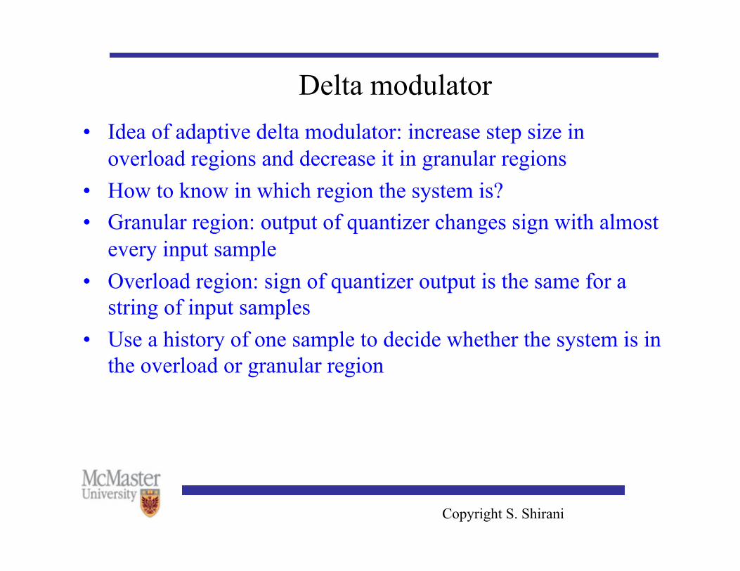
Delta modulator • Idea of adaptive delta modulator: increase step size in
overload regions and decrease it in granular regions • How to know in which region the system is? • Granular region: output of quantizer changes sign with almost
every input sample • Overload region: sign of quantizer output is the same for a
string of input samples • Use a history of one sample to decide whether the system is in
the overload or granular region
Copyright S. Shirani
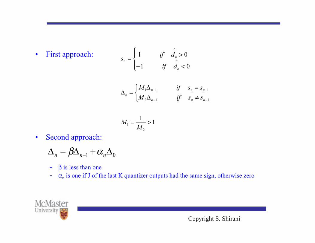
• First approach:
• Second approach:
– β is less than one – αn is one if J of the last K quantizer outputs had the same sign, otherwise zero
Copyright S. Shirani
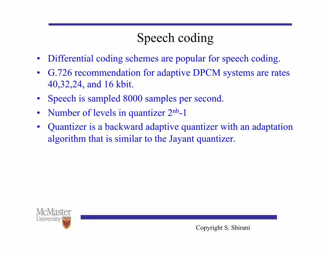
Speech coding • Differential coding schemes are popular for speech coding. • G.726 recommendation for adaptive DPCM systems are rates
40,32,24, and 16 kbit. • Speech is sampled 8000 samples per second. • Number of levels in quantizer 2nb-1 • Quantizer is a backward adaptive quantizer with an adaptation
algorithm that is similar to the Jayant quantizer.