Differentiation (teaching and learning guide 7) - · PDF fileTeaching and Learning Guide 7: Differentiation Page 2 of 42 Table of contents Section 1: Introduction to the guide

METAL Teaching and Learning

Guide 7: Differentiation

Teaching and Learning Guide 7: Differentiation

Page 2 of 42

Table of contents Section 1: Introduction to the guide ................................................................................... 3 Section 2: Differentiation.................................................................................................... 3

1. The concept of differentiation................................................................................................................ 3 2. Presenting the concept of differentiation ............................................................................................... 4 3. Delivering the concept of differentiation to small or larger groups ...................................................... 5 4. Discussion Questions ............................................................................................................................. 9 5. Activities ................................................................................................................................................ 9 6. Top Tips ............................................................................................................................................... 11 7. Conclusion ........................................................................................................................................... 12

Section 3: Practical Applications: Elasticity and Optimisation........................................... 12 1. The concepts of elasticity and optimisation......................................................................................... 12 2. Presenting the concept of elasticity and optimisation.......................................................................... 13 3. Delivering the concept of elasticity and optimisation to small and larger groups............................... 13

Section 4: Discussion........................................................................................................ 15 Topic 1: Total and Marginal Utility......................................................................................................... 15 Topic 2: Cocaine and the Elasticity of Demand ...................................................................................... 16

Section 5: Activities .......................................................................................................... 19 6. Top Tips ............................................................................................................................................... 23

Appendix: Powerpoint slides to help deliver differentiation.............................................. 23


Page 3 of 42

Section 1: Introduction to the guide Differentiation lies at the heart of an introductory module or course in mathematical economics,

but it can present a number of significant challenges to students that need to be dealt with to

ensure they become confident dealing with the rest of their degree course material.

Moving from introductory concepts through to constrained optimisation covers a great deal of

ground and often in a relatively short period of time; a feature that creates an added pressure for

the lecturer whose aim is to ensure all students attain a sound understanding of the subject.

Colleagues may agree that often the mechanics and rules of differentiation do not provide great

difficulty for students – although undergraduate groups are typically contain wide variation in

terms of mathematical ability and confidence - the real challenge often lies in students

developing the confidence and independence to be able to identify which rule or method is

relevant. Perhaps more of an issue though is explaining why “rates of change” matter in

economics and the extent to which differentiation is a key tool of analysis in all areas of the

subject. The following sections attempt to provide some guidance as to how this might be

achieved.

- Colleagues will hopefully concur that that mathematics can be learned through teaching

by demonstration, practice in application and learning by demonstration to others and that

key to this is the use of data and application to economic problems and use of economic

principles to guide the mathematics.

Section 2: Differentiation

1. The concept of differentiation Prior to tackling differentiation, students will have been exposed to linear and non-linear

functions and measuring points of interception and slopes over a long portion of the functions.

By now, they should be comfortable with graphing functions, interpreting equations and having

an understanding of the application of both linear and non-linear forms in a host of economically

meaningful examples. As part of this process, comparative static analysis of changes in

equilibrium will often have been explored, with the consequences of say increased income on a

supply and demand model being examined. This approach is helpful in generating a sense of

how changing one variable can have an impact on other variables and, particular when applying

the mathematical finding to an economic application, how important this is to the outcome.


Page 4 of 42

However, implicit in here is an assumption that we are not focussing on small or marginal

changes but on larger ones. Further, the notion of how the slope of say a demand or supply

curve might affect the outcome of the large change might only have been explored in general

terms without explicit consideration of elasticity. To some extent, differentiation is the means by

which both these features can now be addressed in a formal, mathematical way and thus can be

seen as an extension of previous work rather than an abrupt change in direction which could be

disconcerting to the less confident student.

2. Presenting the concept of differentiation In introducing the section on differentiation, it is important to recognise the difficulties that

students have when dealing with this material. The major issue is the conceptual one mentioned

already in that students often struggle with moving beyond the basic statement that ‘that

differentiation is the slope of a line’. While there is some validity in this statement, it clearly does

not provide the complete sense of the technique or its value to us as economists and if students

do not move beyond this level then difficulties can arise in later extensions of the material. A

related point here is getting students to understand and interpret the information that is

contained in derivative functions.

Once they have started the topic, more specific issues arise. Learning the rules of differentiation

does not present problems for the majority of students but developments from them do. For

example, once they have learned the power rule there are in general no problems with applying

it, but there do appear to be difficulties in knowing how to deal with non-simple powers when

differentiating (e.g. negative powers, fractions). This is highlighted best when considering

examples of Cobb-Douglas utility or production functions and maximisation in such a setting.

Aside from practice it is not obvious how such problems can be dealt with.

In addition, the application of some of the rules can prove to be problematic particularly the

quotient, product and chain rules. The more students can practise examples to refine their

understanding of when and how to apply is probably the best method as it is hard to convey this

in large group, plenary sessions. To some extent, the same could be said for the issue of

elasticities, the one area where differentiation can be shown to have a direct relevance to

economics they might have already encountered in a microeconomics module. With this topic it

would seem a number of problems come together to confound the issue. In part this reflects the


Page 5 of 42

way in which the concept is commonly taught at the introductory level, although it is also the

interpretation of parameters that is most confusing for students. The section on partial

elasticities (see below) gives further indications of how this confusion can be tackled.

3. Delivering the concept of differentiation to small or larger groups The main focus is on the use of graphical analysis to introduce the idea that the slope and shape

of the derived function provides information about the slope and shape of the original function,

and vice versa. This is built around economic topics which they are familiar and which are often

being taught in concurrently running micro- and macro-economics modules. This approach also

helps in identifying more readily the information that might be contained in derivative functions,

for example marginal revenue functions

At the end of Guide a set of slides is provided which offers an overview of differentiation. Below

is an accompanying set of notes and comments to which lecturers might wish to refer when

delivering differentiation.

Notes to support first section of Powerpoint slides

As mentioned in Section 1 above, by the time differentiation is introduced, students have in

general become familiar with interpreting the slope of straight lines from earlier in the course or

module. Thus, a useful starting point to introducing the idea of differentiation is to use previous

knowledge of the straight line as a foundation and to build on this knowledge. This can be done

using a small number of slides within a lecture which can be easily expanded to a tutorial.

The basic idea is to consider how best to measure the slope of a line. To begin with this simply

reiterates the process for the slope of a straight line but is then extended to explore the issue of

the margin of error if the slope of the line was no longer straight but was now curved. Again,

links to the non-linear section of the module can be made explicit here.

A useful place to start is to remind them of the things that they already understand. That is to

discuss finding the slope of a linear function using simple techniques such as plotting and then

reading off co-ordinates to find the lengths of the sides of a triangle. The same approach is then

applied to non-linear functions (see Slide 2)


Page 6 of 42

Having re-stated how to measure a straight line slope, the teaching can move to using the same

idea for the non-linear function above. In doing so it soon becomes apparent that in taking that

approach we are actually measuring the slope of a chord between two points on a curve rather

than measuring the slope of the curve itself. By doing this we can explicitly raise the issue of

measurement error and do so in quite a visual manner.

We take values of points that are on this non-linear function and then use the formula to find the

slope between two points. This process is discussed on the next slide. In doing this we can

show that for the same change in x the change in y that occurs is not constant, can become zero

and then switch in this case to negative. The contrast to linear functions is made very clear. The

final slide we then use plots out the function and the estimated change in the slope. This figure

shows that for some changes in x this appears reasonable, but for others it does not. (See Slide

3)

Moving to Slides 4, 5, 6, & 7, we can see that the value of this approach should be that it

reinforces the difference between linear and non-linear functions we is important anyway, but

more specifically, it shows why we need to have a different approach to measuring slopes in a

non-linear world and hence provides a more intuitive rationale for differentiation being studied.

The second activity builds directly on to the first although again the mode of delivery can be

varied according to your particular class or teaching needs. As mentioned above, it has already

been shown that chords are a particular measure of straight line sections between two points on

a curve. What has not been shown though is whether this approach has a greater or lesser

validity than other measures of a curved line’s slope.

Lecturers could then introduce the discussion of chords and tangents directly and again perhaps

relate this to arc and point elasticities that might have been covered in a concurrent

microeconomics module. This might then lead into a discussion about tangencies versus cords.

The final piece of teaching guidance centres on a small group setting rather than in a lecture.


Page 7 of 42

Students are likely to benefit from working in teams studying how to how to interpret the slope of

the derived function from examining the original and graphical function. Getting students to

practice drawing original functions from what the derived function looks like really aids

understanding of what differentiation is about and what its uses are. By recognising that there is

information contained within the derived functions helps reinforce to students the idea that there

is value in the concept of differentiation.

This is perhaps best done if students draw out the tangency points so that they are interpreting

the slopes of straight lines rather than the non-linear function (in turn reinforcing the relationship

between tangency points and differentiation). There is a slight caveat to this and that is we have

to admit not all students like this but it does help some of the stronger ones who are new to the

topic of differentiation.

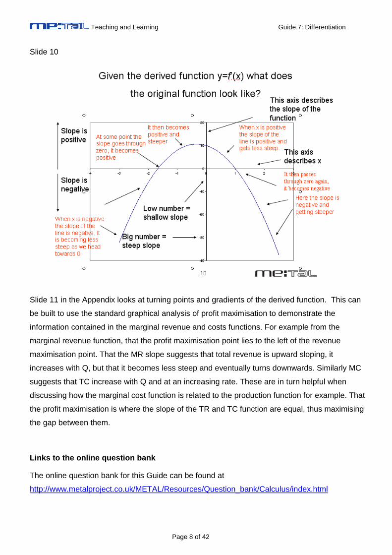
Students can be asked to refer to slides 9 and 10 and consider a non-linear function and

examine what the original function looked like (or the reverse). If you deal with a difficult function

and work through an example there can be a sense of satisfaction to the students that they can

deal with what appeared a complex non-linear function. The following slides describe such an

example.


Page 8 of 42

Slide 10

Slide 11 in the Appendix looks at turning points and gradients of the derived function. This can

be built to use the standard graphical analysis of profit maximisation to demonstrate the

information contained in the marginal revenue and costs functions. For example from the

marginal revenue function, that the profit maximisation point lies to the left of the revenue

maximisation point. That the MR slope suggests that total revenue is upward sloping, it

increases with Q, but that it becomes less steep and eventually turns downwards. Similarly MC

suggests that TC increase with Q and at an increasing rate. These are in turn helpful when

discussing how the marginal cost function is related to the production function for example. That

the profit maximisation is where the slope of the TR and TC function are equal, thus maximising

the gap between them.

Links to the online question bank

The online question bank for this Guide can be found at

http://www.metalproject.co.uk/METAL/Resources/Question_bank/Calculus/index.html


Page 9 of 42

The questions are broken down into 5 sections which focus on the rules of differentiation. These

are ‘self-contained’ and students can work through these once they have learnt the basic rules in

lecture/ tutorial. Students at the lower ability range would probably benefit from working in pairs

and lecturers might want to ask students to discuss why any particular ‘wrong’ answer was not

correct.

Video clips

The video clips can be found at:

http://www.ntu.ac.uk/METAL/Resources/Films/Differential_equations/index.html

They are particularly effective because they tightly link the concept of differentiation to a ‘real-

world’ example. For the first part, lecturers might want to look at the first video clip which

focuses on whether it would be cheaper to educate students if universities were larger using

differentiation to discover the answer. This is extended with an analysis of what happens to the

costs of providing floor space as hotel buildings increase in size, showing how the use of

differentiation can help to make sense of cost decisions

4. Discussion Questions Students could be encouraged to think of examples of ‘everyday variables’ which are negatively

or positively related. For example, the relationship between the number of years experience a

worker has and the salary they can command or the link between the global population size and

the scarcity of economic resources. Students could then consider the strength of the

relationships they have identified. Implicitly, such a discussion would touch upon issues relating

to rates of change.

5. Activities Students will need some basic practice in differentiating economic variables in light of the

PowerPoint presentation and discussion. Discussion of the slides would be a useful and

straightforward activity for tutorial.


Page 10 of 42

ACTIVITY ONE

Learning Objectives

LO1: Students learn how to independently calculate simple derivatives

LO2: Students learn some of the real world applicat ions of differentiation

Task One

The following 5 functions are observed as possible relationships between income (Y) and

investment (I) in 5 EU states. In each case you need to calculate the rate of change between

investment and income i.e. I

Y

∂∂

State 1: Y = I5

State 2: Y = I3

State 3: Y= 12I2

State 4: Y=6

State 5: Y=I

5

Task Two

LO1: Students to learn how to graph functions

LO2: Students learn how to interpret a derived func tion.

Students can refer to the Powerpoint slides, particularly Slide 7.

To begin, draw out a (non-linear) function, then underneath introduce the axis in which you plan

to draw the derived function. Crucial here is an interpretation of what the number on both the

axes, and in particular the y axis, actually mean. Students can then trace out what the derived

function will look like using the original function as the values of x change.


Page 11 of 42

ANSWERS

ACTIVITY ONE

Task One

State 1: 45II

Y =∂∂

State 2: 23II

Y =∂∂

State 3: II

Y24=

∂∂

State 4: 0=∂∂

I

Y

State 5: 2

5

II

Y −=∂∂

Task Two

Indeterminate number of answers and outcomes.

6. Top Tips

Students need to have a good sense of the economic applications of differentiation.

They can start by reflecting on their personal ‘variables’ and to consider the strength of

these relationships e.g. between weight and height, rates of interest and borrowing.

Students will probably find it easy to understand that to find ‘marginal’ or

‘maximum/minimum’ points they need to differentiate, but lack any insight as to what

they are doing. For example, when asked to calculate the minimum of the marginal cost

function some doubt whether such an act is even possible. The challenge here is to

provide good examples – provided by students where possible – to contextualise the

mathematics.


Page 12 of 42

7. Conclusion The interpretation of results is also important when considering second differentials and what

exactly they mean when they have been calculated. Again, experience suggests that students

can handle the process of first and second order differentiation relatively easily (given the

caveats of the specific problems above) but they have greater problems knowing what the

numbers mean and what the economics interpretation of them is. Perhaps the final point to

make in terms of common errors is in terms of the examination where a common problem

occurs in simply finding maxima or minima for a function, which might reflect the lack of

understanding of the concept in the first place and hence brings us back to the first issue raised

here.

Section 3: Practical Applications: Elasticity and O ptimisation

1. The concepts of elasticity and optimisation Students seem to have great difficulty with understanding the concept of elasticity. In part this

perhaps reflects a reliance on the visual concept, for example they have less trouble when get to

partial elasticities (which of course are very difficult to visualise), but also because of lazy

terminology by teachers and lecturers . Too often in their initial introduction to economics

students are shown linear demand function that have different slopes and are told that they are

examples of elastic or inelastic demand. Hence they look at the slope of the linear demand

function and use it to interpret elasticity.

This interpretation of elasticity as ‘something to do with the slope’ then comes into conflict with

the concept that the elasticity varies over the slope of a straight line demand function for

example. If elasticity is something to do with the slope how can at the same time its value vary

over the function? This leads to confusion (and in some cases panic) about what the idea of

elasticity is, little engagement with the uses of elasticity, and poor performance on this topic in

exams.

Equally, issues regarding optimisation can frequently trouble students. Although they

understand terms such as ‘minimum’ and ‘maximum’ the real value is helping them to

understand why these are such powerful concepts and tools in economics.


Page 13 of 42

2. Presenting the concept of elasticity and optimisation The Appendix provides some slides which help to show that comparisons of elasticity are

relative at each and every price. The basic structure of the slides introduces the idea that the

elasticity varies over a straight line demand function (and how) and from there to describe how

for any given price we can say that one demand function is more or less elastic than another. A

comment is not provided for each slide – they should be straightforward and pretty much self-

explanatory – but a few helpful pointers are set out below.

Lecturers could use these slides to raise issues of calculating minima and maxima. The graphs

clearly show not just rates of change but ‘peaks’ and ‘troughs’. Reference could be made to

business cycle and students might want to explore how GDP has varied over time and overlay

lines of best fit using Excel

Slide 11 confirms this with a simple diagram and relates to the earlier work on differentials.

Slide 12 attempts to explain how the PED formula ‘works’ by looking at the ration of P and Q and

this is extended with a graphical overview of elasticity along linear functions in Slide 13. The

next slides (Slide 14) consolidates this with worked examples of PED. Slide Sixteen: Here we

rely on the intuition drawn from the previous slide to show the main purpose of this set of slides:

comparisons of elasticity are relative for each price. Slide Seventeen: This slide tries to

demonstrate the above for a particular point on the demand schedules.

3. Delivering the concept of elasticity and optimisation to small and larger groups Perhaps one good way to introduce the concept is to give examples from the world of

economics. For example, students could consider the “The Elasticity of the Demand for Murder”

This example comes from Mark Zupan, University of Rochester (US) and focuses on an

application of elasticity to a somewhat unusual “market”. One of the issues students face is the

intuition underlying calculations of elasticity. As mentioned above, their ability to undertake the

manipulation of differentiation using the given rules is not a problem but their understanding of

the underlying economics can be limited.


Page 14 of 42

In a small group setting (although this can be used as a lecture activity too) introducing the

notion of application can be a way into this unusual example. The market needs to be

considered from a demand point of view first and show how different groups can have very

different conceptualizations of the demand curve. For example, some people might suggest

murder is an irrational act and it would be committed regardless of the potential price the

murderer faces. The question can then be posed as to how the demand curve would look and

what the elasticity of demand would be a given “price”? The demand curve is perfectly inelastic,

with quantities of murders on the horizontal axis and the sentence served (price) on the vertical

axis. The elasticity is of course zero.

Then a second question can be posed. What if there are other views about murder – for

example, what if other people say murderers are rational and respond to the price of committing

such crimes. The same two questions can be posed – what is the demand curve like and also

what is the elasticity at these points? To answer the latter assume that 30,000 murders are

committed per year if the average sentence served is 20 years, but the murder rate rises to

45,000 annually if the average prison term is only 15 years. Assume that 50% of murderers are

caught in either case.

This topic uses the principles of economics applied in a non-standard setting. In so doing it

forces the student to think what the concept of price and quantity mean and whether economics

can provide insight in all situations. This reinforces the understanding of the concept of elasticity

and provides practice of the mathematical tools used to calculate them.

Lecturers could choose to build upon this analysis to explore issues concerning optimisation.

For example by introducing the idea of revenue and then moving to marginal revenue and

revenue maximisation. Students could look at variables which they seek to maximise – such as

income or long-term income earning potential or grades un university finals – and compare

against other variables which they try to minimise – food wastage, council tax bills etc.


Page 15 of 42

Links to the online question bank

There some very good ‘applied’ questions to support this Guide at:

http://www.metalproject.co.uk/METAL/Resources/Question_bank/Economics%20applications/in

dex.html

Elasticity questions may also be found at:

http://www.metalproject.co.uk/METAL/Resources/Question_bank/Economics%20applications/in

dex.html in addition to questions which focus on optimisation problems.

Video clips

Video clips can be found at

http://www.ntu.ac.uk/METAL/Resources/Films/Differential_equations/index.html and although

the clips do not focus on elasticity and/or optimisation per se they could be linked with the

second set of films which look at differential equations.

Section 4: Discussion The material that can be used to frame discussion topics can be quite varied in nature and

although dealing with quite a specific, technical area, they can provide a rich source of

understanding for students.

Topic 1: Total and Marginal Utility Introduction: This comes from David Gillette and Robert delMass1 and is one that appears to

have been used in a number of small group settings quite successfully. Relating total and

marginal concepts is sometimes difficult for students and while they might be able to show how

to derive this mathematically using differentiation, they do no always have the intuition behind it.

Using total and marginal utility as vehicle and based on personal consumption habits is one way

in which to draw the students in to the area in a fun manner.

1 Gillette, David and Robert delMas. "Psycho-Economics: Studies in Decision Making." Classroom Expernomics, 1(2), Fall 1992, pp. 5-6


Page 16 of 42

Discussion: in a sense this is a mixture between activity and discussion but does require the

activity to be part of the process. Students are initially introduced to the notion of measuring

changes in welfare of the individual and to what extent we can do this as economists. We could

begin with the notion of defining economics as a science aiming to improve the welfare of

society but with what tools and how accurately can this be done? The discussion can then very

quickly be brought to the specific case of the individual consumer and how his or her welfare

changes.

Students in the group are asked to give themselves a percentage mark on how they feel at

present on the basis that 0 means pretty awful and 100 is fantastic. The next step is then to give

them a sweet each one at a time and then get the students to rate themselves again and to write

it down. Very quickly you get a dataset of information on total and marginal utility (on a

percentage scale of course) and there should be clear evidence of diminishing marginal utility as

consumption rises.

The next step is then to provide the students with some examples of utility functions, perhaps

simple ones to begin with and then move onto more complex such as Cobb-Douglas form ones

to show how an individual’s utility depends on the consumption of more than one good (i.e.

sweets) and derive marginal utilities for these functions .

Conclusions: the major value of this approach is in linking explicitly the notions of total and

marginal functions on the basis of primary data collection in an area that students are familiar

with. At the end of the process, students should be able to undertake differentiation of both

simple and more advanced utility functions and thus be able to apply the technique to similar

functions in other areas such as production functions.

Topic 2: Cocaine and the Elasticity of Demand This is an example drawn from Michael Kuehlwein, Pomona College in the US. Occasionally it is

worth choosing examples that in some senses shock the students, on the basis that they may

remember the concept by drawing on their memory of the example. One such topic is the use of

drugs.


Page 17 of 42

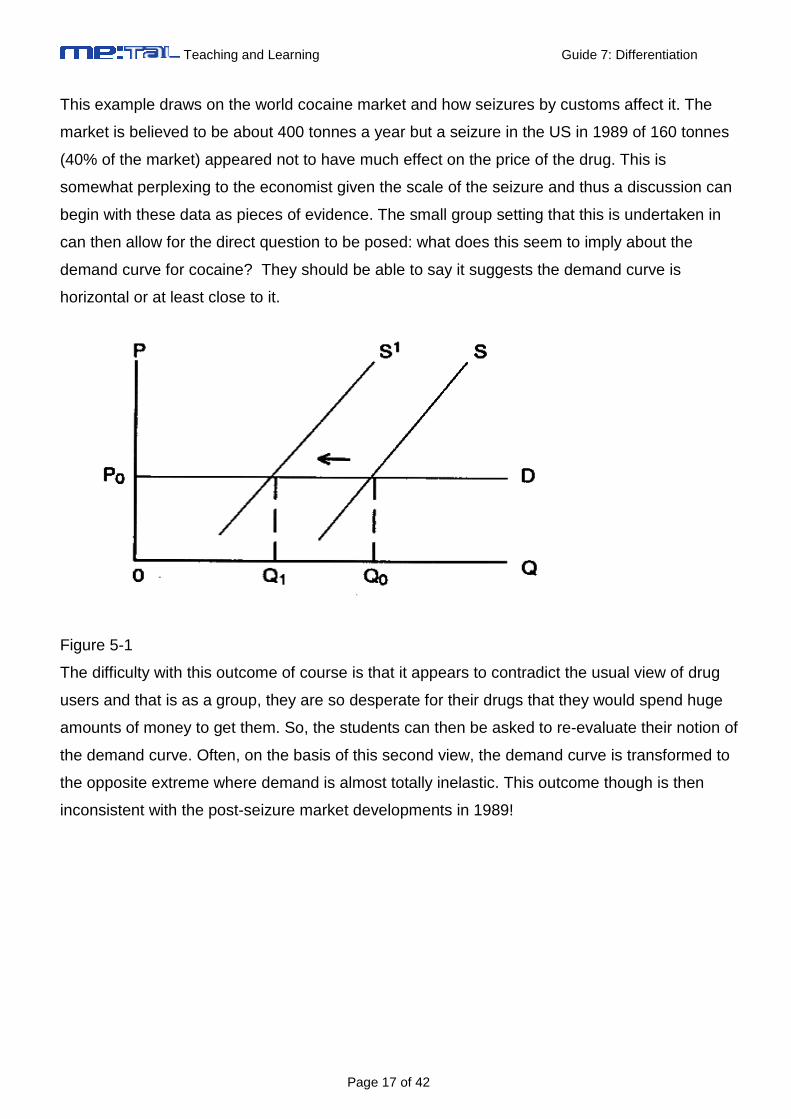
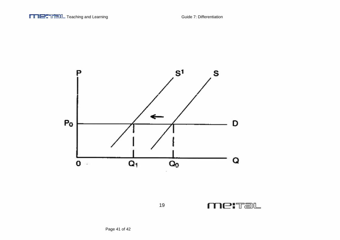
This example draws on the world cocaine market and how seizures by customs affect it. The

market is believed to be about 400 tonnes a year but a seizure in the US in 1989 of 160 tonnes

(40% of the market) appeared not to have much effect on the price of the drug. This is

somewhat perplexing to the economist given the scale of the seizure and thus a discussion can

begin with these data as pieces of evidence. The small group setting that this is undertaken in

can then allow for the direct question to be posed: what does this seem to imply about the

demand curve for cocaine? They should be able to say it suggests the demand curve is

horizontal or at least close to it.

Figure 5-1

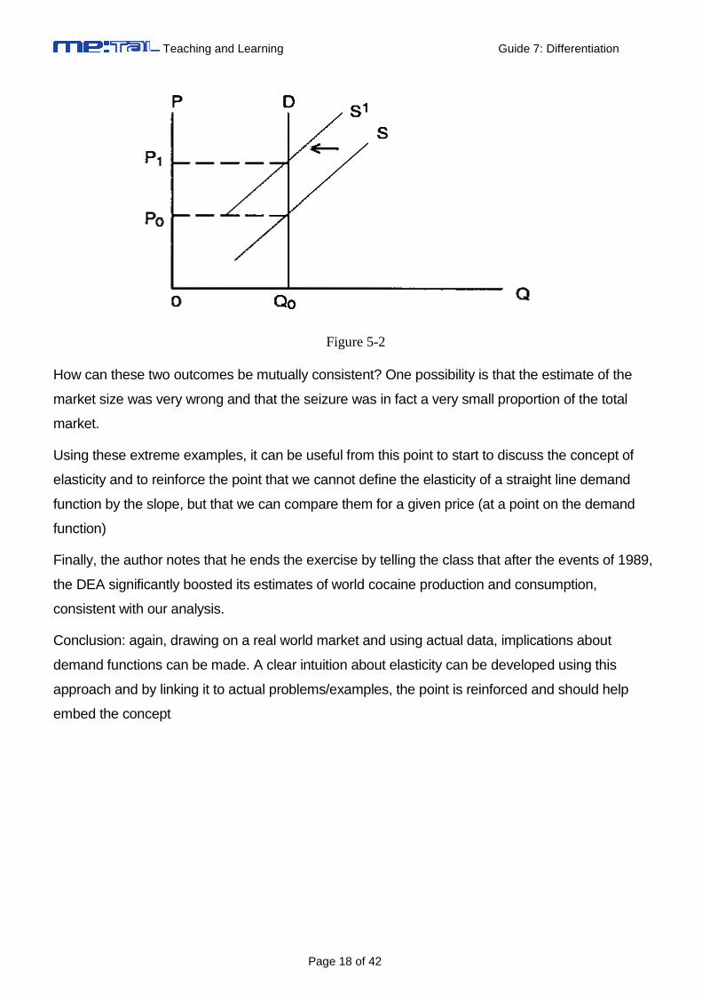
The difficulty with this outcome of course is that it appears to contradict the usual view of drug

users and that is as a group, they are so desperate for their drugs that they would spend huge

amounts of money to get them. So, the students can then be asked to re-evaluate their notion of

the demand curve. Often, on the basis of this second view, the demand curve is transformed to

the opposite extreme where demand is almost totally inelastic. This outcome though is then

inconsistent with the post-seizure market developments in 1989!


Page 18 of 42

Figure 5-2

How can these two outcomes be mutually consistent? One possibility is that the estimate of the

market size was very wrong and that the seizure was in fact a very small proportion of the total

market.

Using these extreme examples, it can be useful from this point to start to discuss the concept of

elasticity and to reinforce the point that we cannot define the elasticity of a straight line demand

function by the slope, but that we can compare them for a given price (at a point on the demand

function)

Finally, the author notes that he ends the exercise by telling the class that after the events of 1989,

the DEA significantly boosted its estimates of world cocaine production and consumption,

consistent with our analysis.

Conclusion: again, drawing on a real world market and using actual data, implications about

demand functions can be made. A clear intuition about elasticity can be developed using this

approach and by linking it to actual problems/examples, the point is reinforced and should help

embed the concept


Page 19 of 42

Section 5: Activities ACTIVITY ONE: The ‘Horse Race’ Game

Learning objectives

LO1: Students learn how to solve simple problems in volving differentiation.

LO2: Students learn how to work independently and i n small teams to answer problems

concerning ‘applied differentiation’.

Understanding and learning mathematics requires practice on the part of students. This

understandably can be a boring task to undertake. To make it more interesting an element of

competition can often be useful.

The horse race game operates under a quiz format in which students race to answer questions

presented to them. The game speeds up somewhat if these are asked as multiple choice

questions. This format can be used to look at issues regarding respect to cost, revenue and

profit functions which lend themselves to the idea of being broken into stages. For example, a

set of questions taken from a standard format used in problem classes breaks neatly into 10

stages.

A horse represents a group of students. The number of horses in the race can obviously be

varied with the size of the class and students often enjoy coming up with names for their horses.

The only thing to remember is to set enough questions so that one team can complete the race.

Task One

Let P = 20 – 5Q be a demand function

a. how many units will the firm sell if the price is 15?

b. what price should the firm set if it wants to sell 3 units?

c. compute the marginal revenue corresponding to this function

d. calculate price elasticity of demand when price moves from 1 to 3.

e. what is the relationship between the slope of the demand curve and the price

elasticity of demand?

f. Calculate the total revenue function for the firm and find its maximum


Page 20 of 42

Task Two

A firms total revenue function is given as follows,

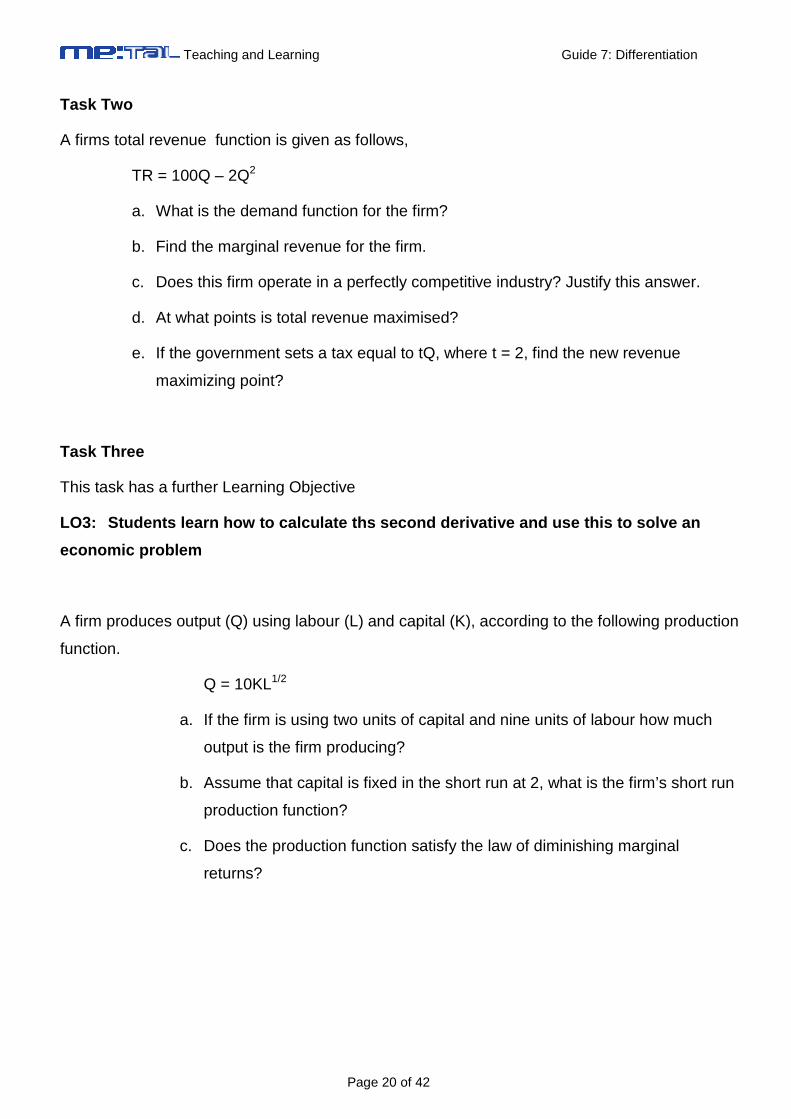
TR = 100Q – 2Q2

a. What is the demand function for the firm?

b. Find the marginal revenue for the firm.

c. Does this firm operate in a perfectly competitive industry? Justify this answer.

d. At what points is total revenue maximised?

e. If the government sets a tax equal to tQ, where t = 2, find the new revenue

maximizing point?

Task Three

This task has a further Learning Objective

LO3: Students learn how to calculate ths second der ivative and use this to solve an

economic problem

A firm produces output (Q) using labour (L) and capital (K), according to the following production

function.

Q = 10KL1/2

a. If the firm is using two units of capital and nine units of labour how much

output is the firm producing?

b. Assume that capital is fixed in the short run at 2, what is the firm’s short run

production function?

c. Does the production function satisfy the law of diminishing marginal

returns?


Page 21 of 42

ANSWERS

ACTIVITY ONE

Task One

a. Q=1

b. P=5

c. QQ

TRMR 1020 −=

∂∂=

d. PeD = 053.0%1002

%100192

%

%=

×+

×−=

∆∆

=P

Qη

e. The price elasticity varies as we move along the demand curve. The ped falls as

we move from left to right.

f.

10

20

2

02010

max

520

5202

=⇒

=⇒

=⇒

=−=∂∂

−=

−=

P

TR

Q

qQ

TR

TRstQ

QQTR

QP

Task Two

a. QPAR 2100 −==

b. QQQ

TRMR 41004100 −=−=

∂∂=

c. No because MRAR≠

d. 25Q when MR max =

e. Tax of tQ where t =2

66.16

1006

24100

−=

−−=

Q

Q

QQMR


Page 22 of 42

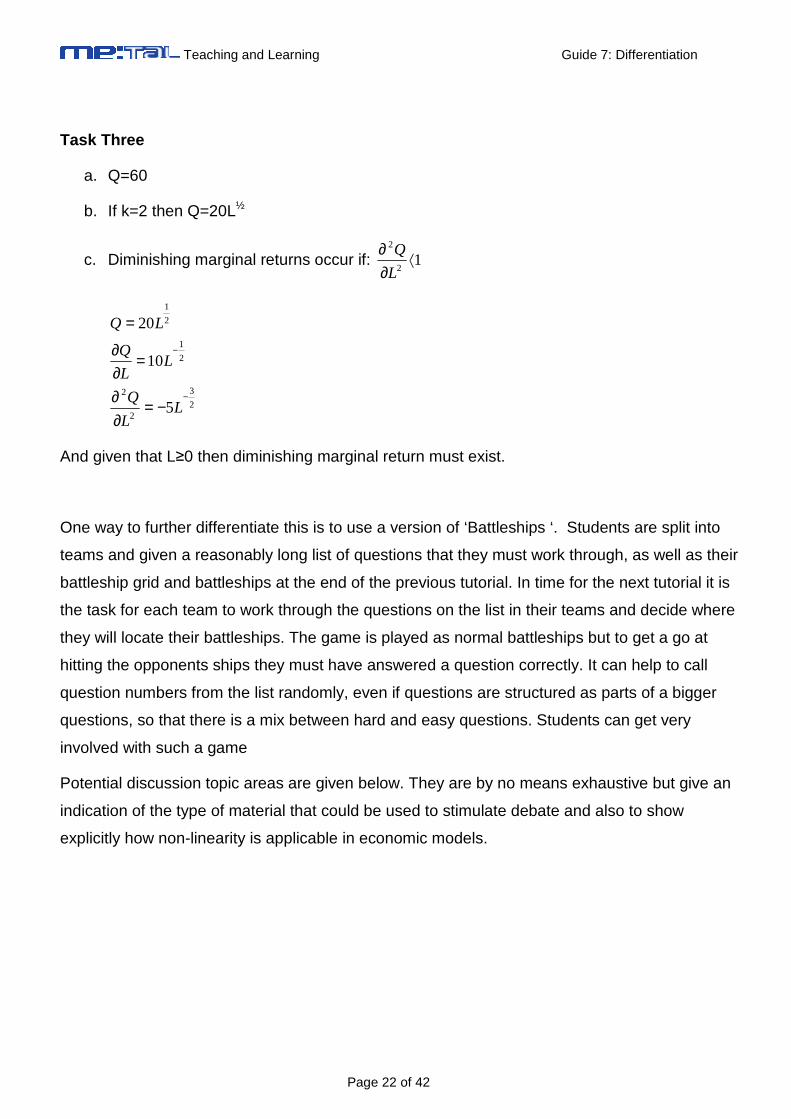
Task Three

a. Q=60

b. If k=2 then Q=20L½

c. Diminishing marginal returns occur if: 12

2

⟨∂∂

L

Q

2

3

2

2

2

1

2

1

5

10

20

−

−

−=∂∂

=∂∂

=

LL

Q

LL

Q

LQ

And given that L≥0 then diminishing marginal return must exist.

One way to further differentiate this is to use a version of ‘Battleships ‘. Students are split into

teams and given a reasonably long list of questions that they must work through, as well as their

battleship grid and battleships at the end of the previous tutorial. In time for the next tutorial it is

the task for each team to work through the questions on the list in their teams and decide where

they will locate their battleships. The game is played as normal battleships but to get a go at

hitting the opponents ships they must have answered a question correctly. It can help to call

question numbers from the list randomly, even if questions are structured as parts of a bigger

questions, so that there is a mix between hard and easy questions. Students can get very

involved with such a game

Potential discussion topic areas are given below. They are by no means exhaustive but give an

indication of the type of material that could be used to stimulate debate and also to show

explicitly how non-linearity is applicable in economic models.


Page 23 of 42

6. Top Tips

Appendix: Powerpoint slides to help deliver differe ntiation. These Powerpoint slides are provided below in a ‘static’ format. They can also be downloaded

from the METAL website at

http://www.ntu.ac.uk/METAL/Resources/Teaching_learning/index.html. The slides are ‘built up’

so colleagues can use simple animation to create an effective presentation.

© Authored and Produced by the METAL Project Consortium 2007

Using extreme examples can grab student’s attention of a topic and may help them to

remember the concept. The trick is to identify where they might have best value, and not

to use them too often.

2

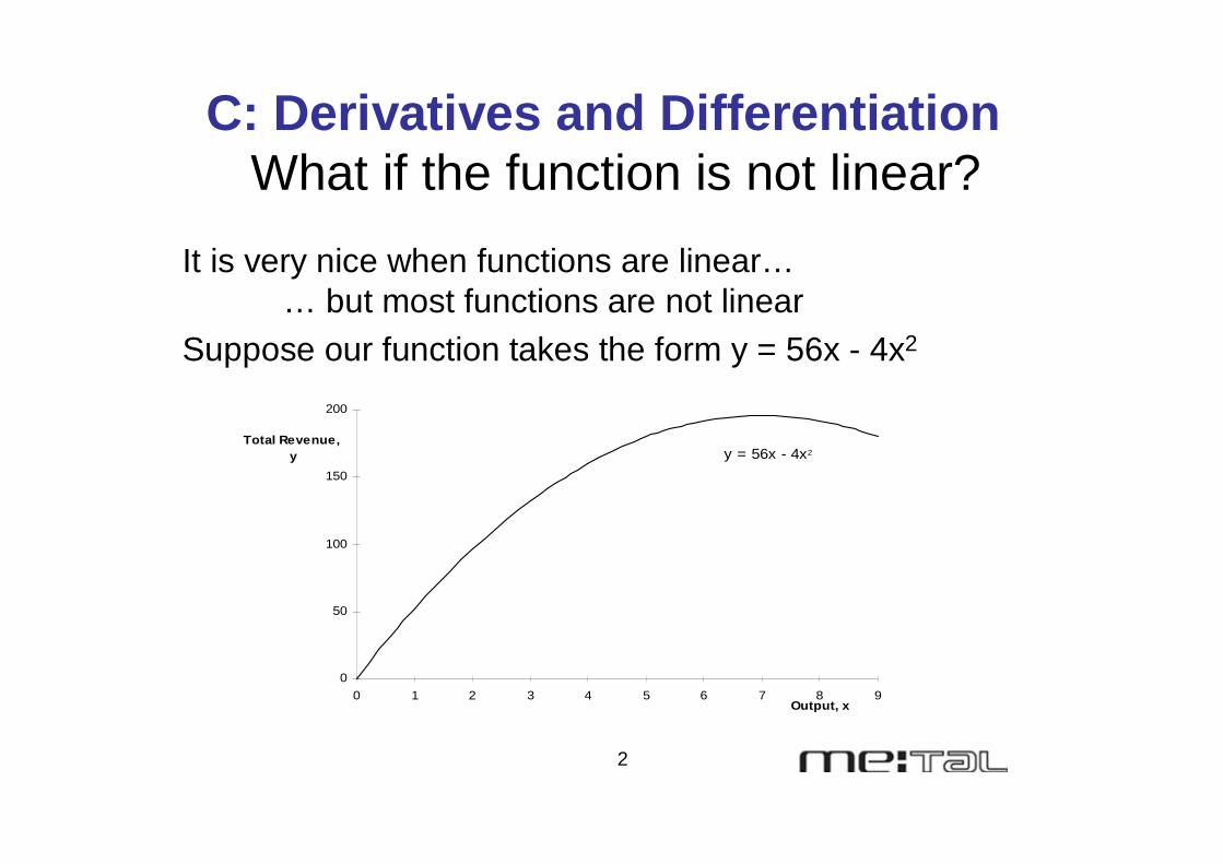
What if the function is not linear?

0

50

100

150

200

0 1 2 3 4 5 6 7 8 9Output, x

Total Revenue, y y = 56x - 4x2

It is very nice when functions are linear…… but most functions are not linear

Suppose our function takes the form y = 56x - 4x2

C: Derivatives and Differentiation

3

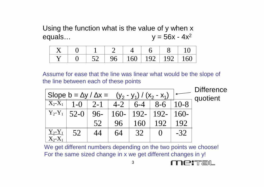
Using the function what is the value of y when x equals… y = 56x - 4x2

Slope b = ∆y / ∆x = (y2 - y1) / (x2 - x1)

Assume for ease that the line was linear what would be the slope of the line between each of these points

X 0 1 2 4 6 8 10Y 0 52 96 160 192 192 160

We get different numbers depending on the two points we choose!For the same sized change in x we get different changes in y!

X2-X1 1-0 2-1 4-2 6-4 8-6 10-8 Y2-Y1 52-0 96-

52 160-96

192-160

192-192

160-192

Y2-Y1

X2-X1 52 44 64 32 0 -32

Difference quotient


Page 26 of 42

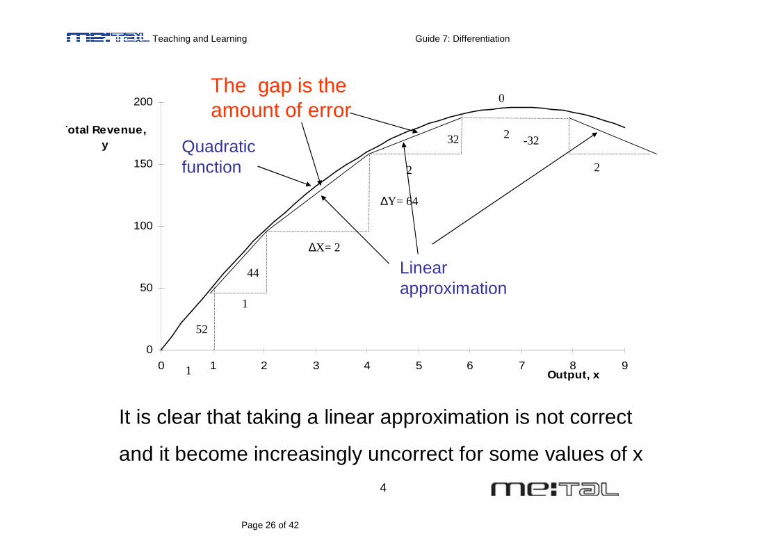
4

0

50

100

150

200

0 1 2 3 4 5 6 7 8 9Output, x

Total Revenue, y

1

1

∆X= 2

2

2

2

52

44

∆Y= 64

32

0

-32

It is clear that taking a linear approximation is not correct

and it become increasingly uncorrect for some values of x

The gap is the amount of error

Quadratic function

Linear approximation


Page 27 of 42

5

0

50

100

150

200

0 1 2 3 4 5 6 7 8 9Output, x

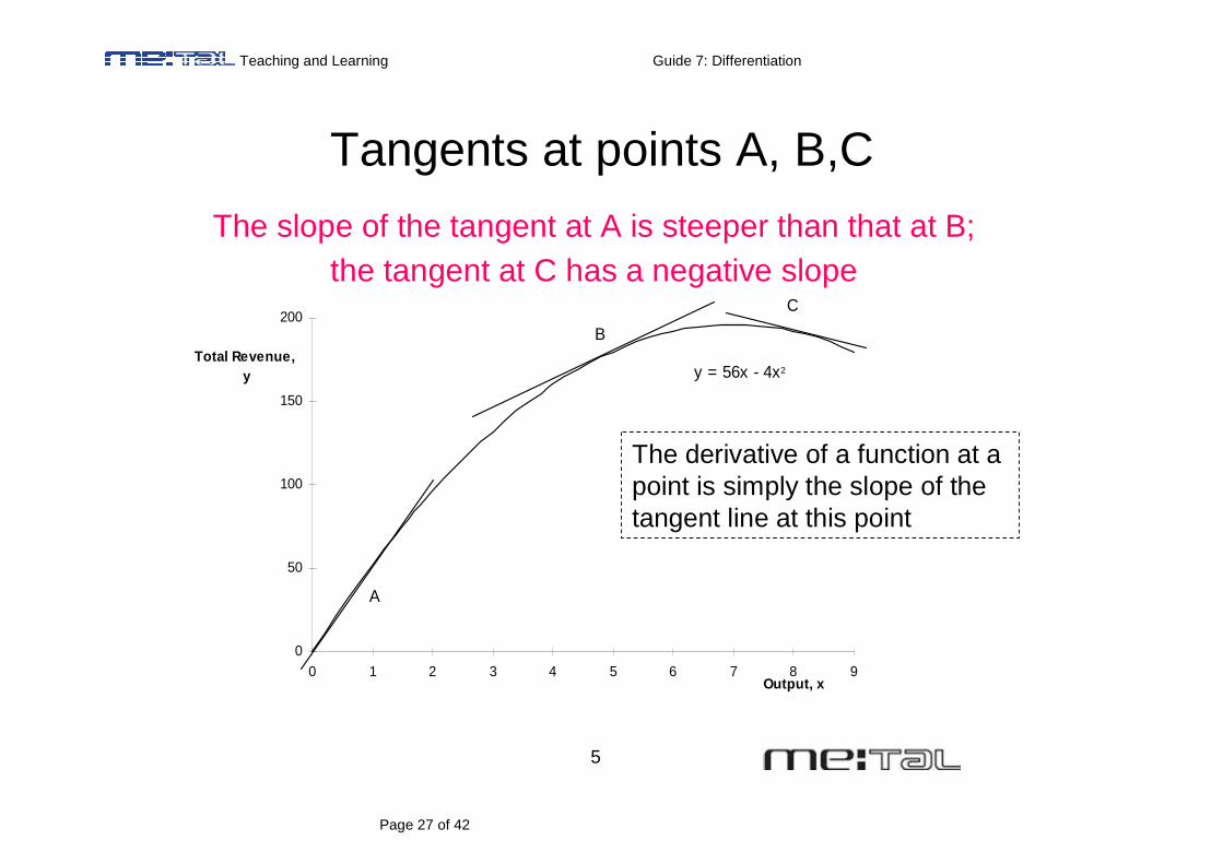
Total Revenue, y y = 56x - 4x2

A

B

C

Tangents at points A, B,C

The slope of the tangent at A is steeper than that at B; the tangent at C has a negative slope

The derivative of a function at a point is simply the slope of the tangent line at this point


Page 28 of 42

6

x

y

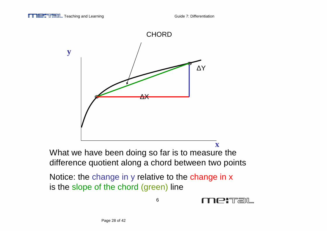
What we have been doing so far is to measure the difference quotient along a chord between two points

Notice: the change in y relative to the change in xis the slope of the chord (green) line

∆Y

∆X

CHORD


Page 29 of 42

7

x

y

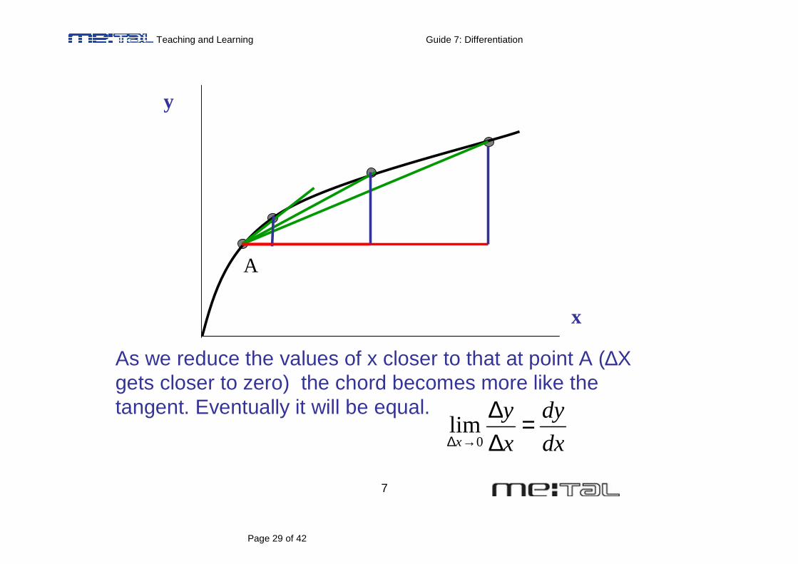
As we reduce the values of x closer to that at point A (∆X gets closer to zero) the chord becomes more like the tangent. Eventually it will be equal.

A

dx

dy

x

yx

=∆∆

→∆ 0lim


Page 30 of 42

8

0

50

100

150

200

0 1 2 3 4 5 6 7 8 9Output, x

Total Revenue, y

y = 56x - 4x2

A

B

C

-20

-10

0

10

20

30

40

50

60

0 1 2 3 4 5 6 7 8 9

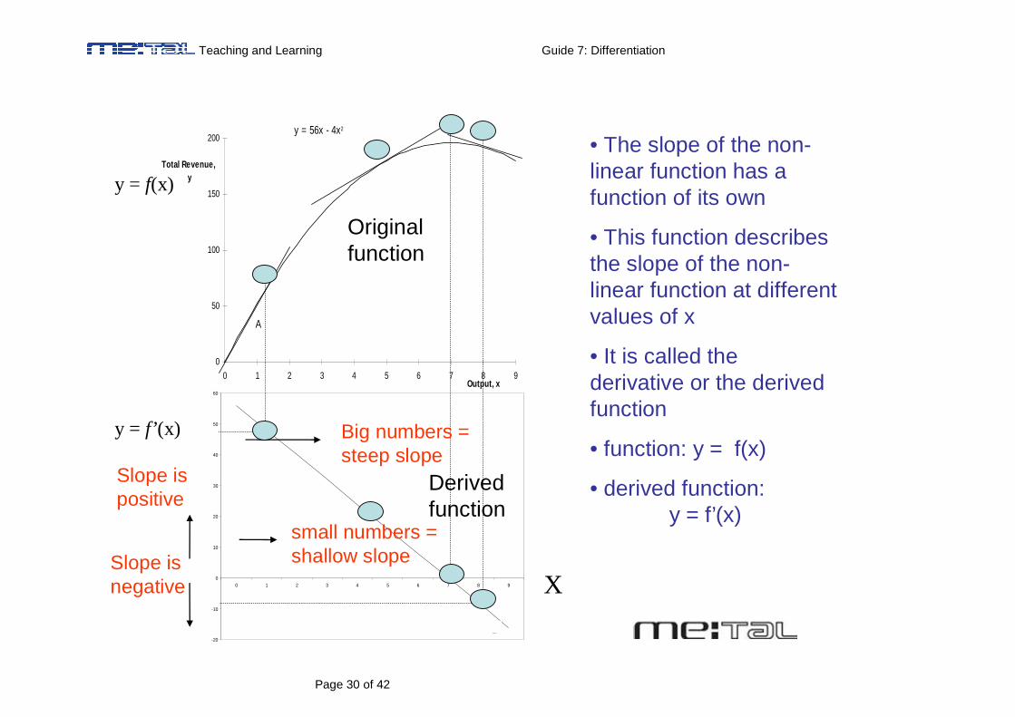
• The slope of the non-linear function has a function of its own

• This function describes the slope of the non-linear function at different values of x

• It is called the derivative or the derived function

• function: y = f(x)

• derived function: y = f’(x)

X

y = f’ (x)

y = f(x)

Slope is positive

Slope is negative

Big numbers = steep slope

small numbers = shallow slope

Original function

Derived function


Page 31 of 42

9

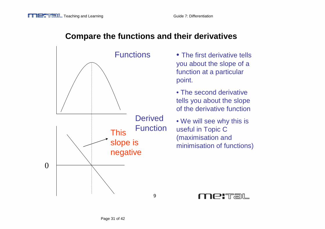
Compare the functions and their derivatives

Functions

Derived Function

0

This slope is negative

• The first derivative tells you about the slope of a function at a particular point.

• The second derivative tells you about the slope of the derivative function

• We will see why this is useful in Topic C (maximisation and minimisation of functions)


Page 32 of 42

10

-40

-30

-20

-10

0

10

20

-4 -3 -2 -1 0 1 2 3

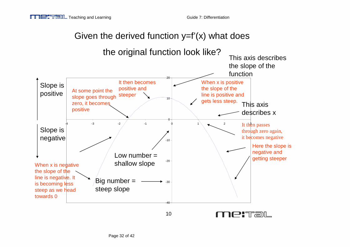
Given the derived function y=f’(x) what does

the original function look like?

When x is negative the slope of the line is negative. It is becoming less steep as we head towards 0

At some point the slope goes through zero, it becomes positive

It then becomes positive and steeper

When x is positive the slope of the line is positive and gets less steep.

It then passes through zero again, it becomes negative

Here the slope is negative and getting steeper

Slope is positive

Slope is negative

Big number = steep slope

Low number = shallow slope

This axis describes the slope of the function

This axis describes x


Page 33 of 42

11-15

-10

-5

0

5

10

15

-4 -3 -2 -1 0 1 2 3

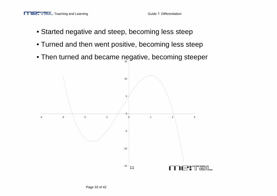
• Started negative and steep, becoming less steep

• Turned and then went positive, becoming less steep

• Then turned and became negative, becoming steeper


Page 34 of 42

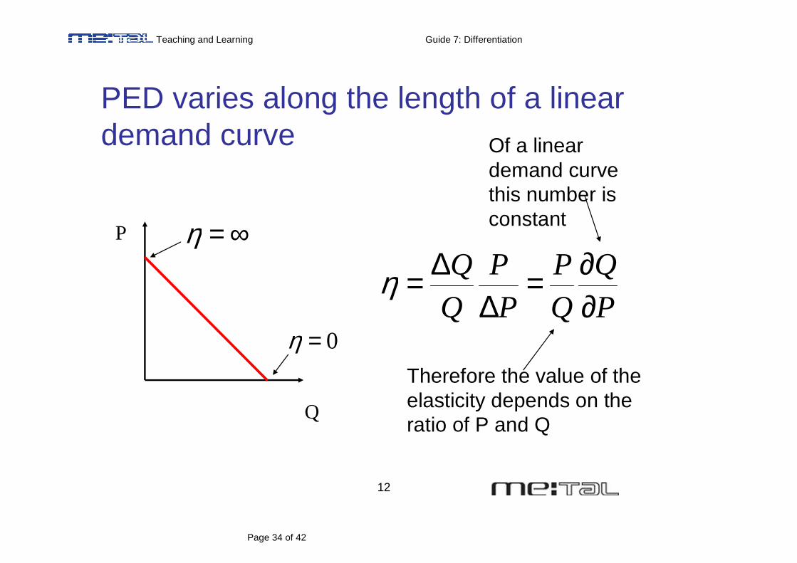
12

PED varies along the length of a linear demand curve

Q

P ∞=η

0=ηP

Q

Q

P

P

P

Q

Q

∂∂=

∆∆=η

Of a linear demand curve this number is constant

Therefore the value of the elasticity depends on the ratio of P and Q


Page 35 of 42

13

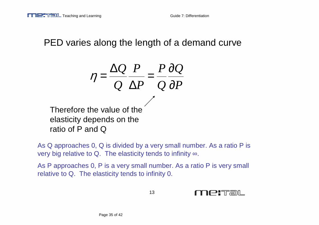
PED varies along the length of a demand curve

P

Q

Q

P

P

P

Q

Q

∂∂=

∆∆=η

Therefore the value of the elasticity depends on the ratio of P and Q

As Q approaches 0, Q is divided by a very small number. As a ratio P is very big relative to Q. The elasticity tends to infinity ∞.

As P approaches 0, P is a very small number. As a ratio P is very small relative to Q. The elasticity tends to infinity 0.


Page 36 of 42

14

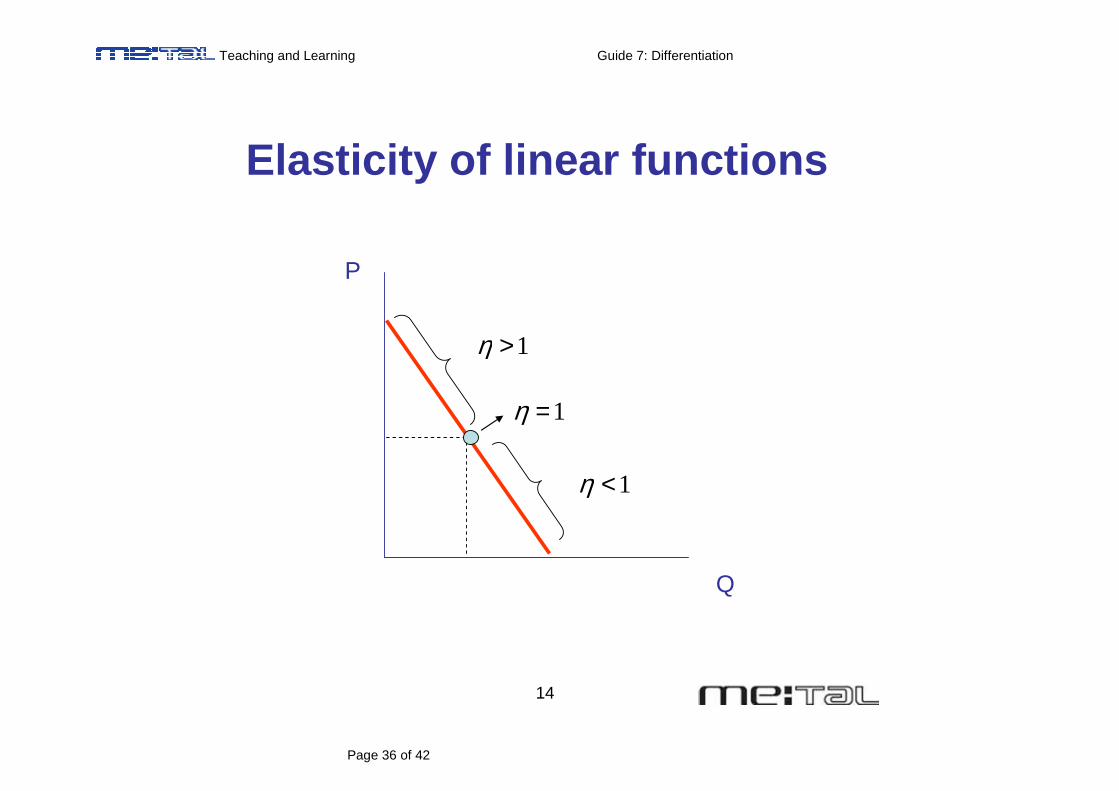
Elasticity of linear functions

Q

P

1=η

1>η

1<η


Page 37 of 42

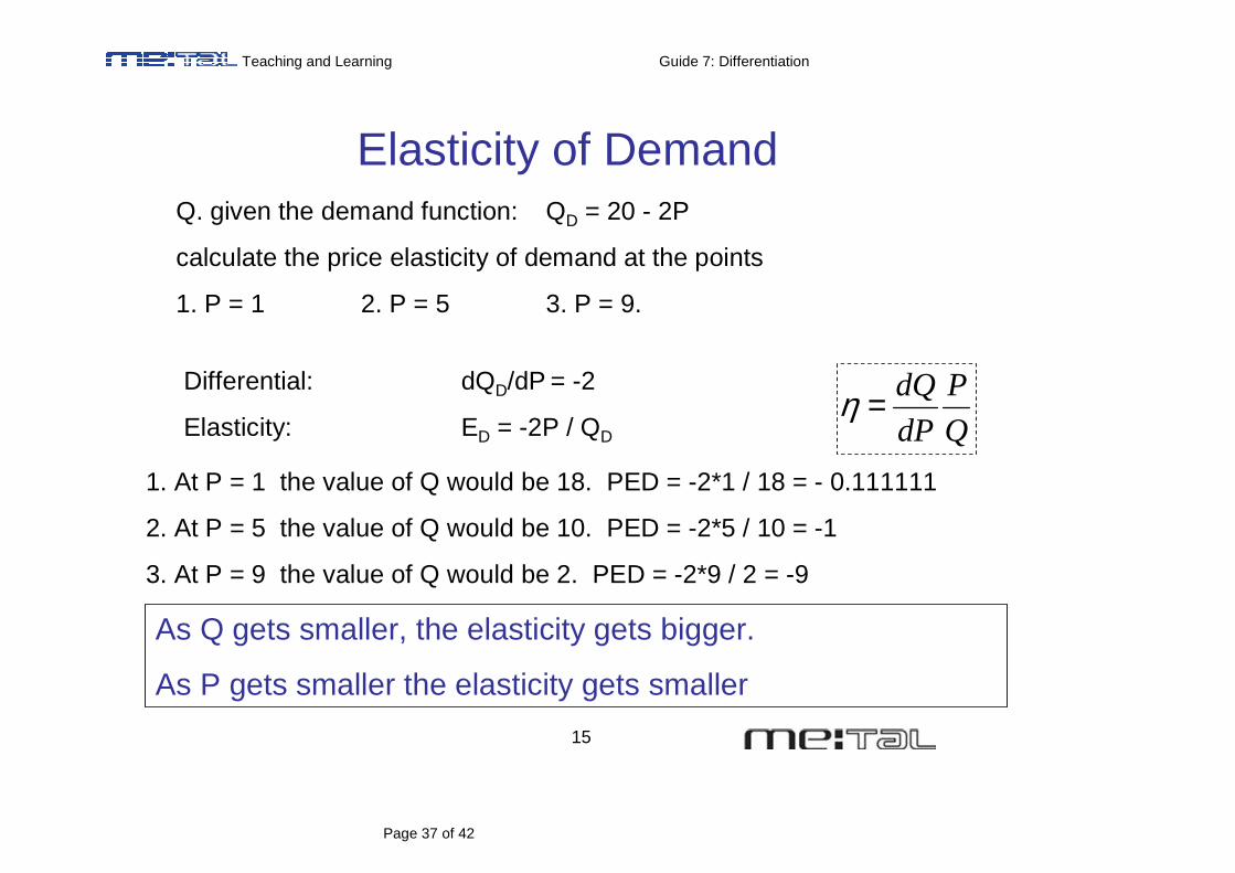
15

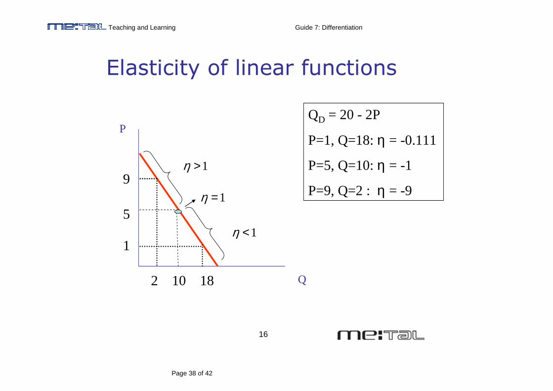
Elasticity of DemandQ. given the demand function: QD = 20 - 2P

calculate the price elasticity of demand at the points

1. P = 1 2. P = 5 3. P = 9.

Differential: dQD/dP = -2

Elasticity: ED = -2P / QD

1. At P = 1 the value of Q would be 18. PED = -2*1 / 18 = - 0.111111

2. At P = 5 the value of Q would be 10. PED = -2*5 / 10 = -1

3. At P = 9 the value of Q would be 2. PED = -2*9 / 2 = -9

Q

P

dP

dQ=η

As Q gets smaller, the elasticity gets bigger.

As P gets smaller the elasticity gets smaller


Page 38 of 42

16


Q

P

1=η

1>η

1<η

2 10 18

1

5

9

QD = 20 - 2P

P=1, Q=18: η = -0.111

P=5, Q=10: η = -1

P=9, Q=2 : η = -9


Page 39 of 42

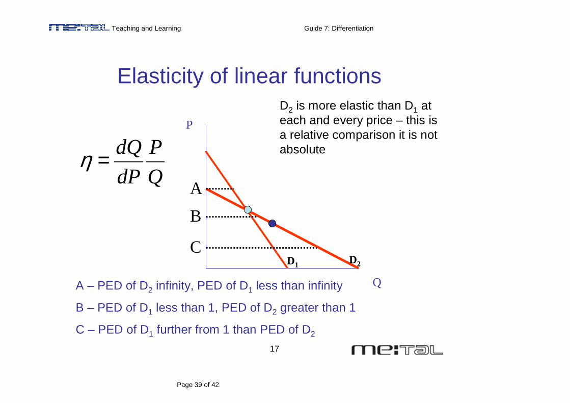
17


Q

P

D1 D2

A

B

C

A – PED of D2 infinity, PED of D1 less than infinity

B – PED of D1 less than 1, PED of D2 greater than 1

C – PED of D1 further from 1 than PED of D2

D2 is more elastic than D1 at each and every price – this is a relative comparison it is not absolute

Q

P

dP

dQ=η


Page 40 of 42

18

Q

P

dP

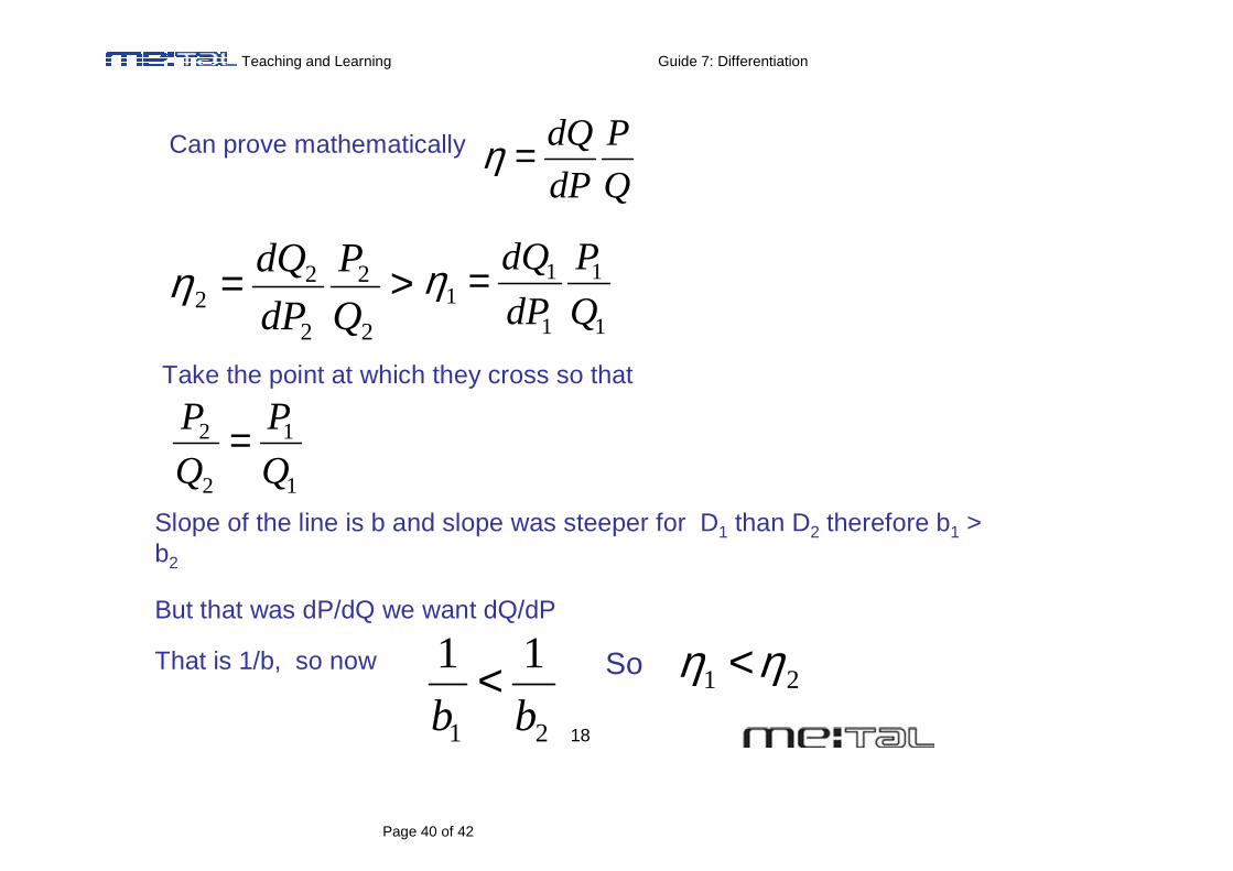
dQ=ηCan prove mathematically

>=2

2

2

22 Q

P

dP

dQη1

1

1

11 Q

P

dP

dQ=η

Take the point at which they cross so that

1

1

2

2

Q

P

Q

P =

Slope of the line is b and slope was steeper for D1 than D2 therefore b1 > b2

But that was dP/dQ we want dQ/dP

That is 1/b, so now

21

11

bb< So 21 ηη <


Page 41 of 42

19


Page 42 of 42

20

Documents

Differentiation (teaching and learning guide 7) - · PDF fileTeaching and Learning Guide 7: Differentiation Page 2 of 42 Table of contents Section 1: Introduction to the guide