Embed Size (px)
Citation preview
21 May 2013
Diffraction geometry parameterisation and refinement
David WatermanCCP4
Cambridge 22 May 2013
21 May 2013
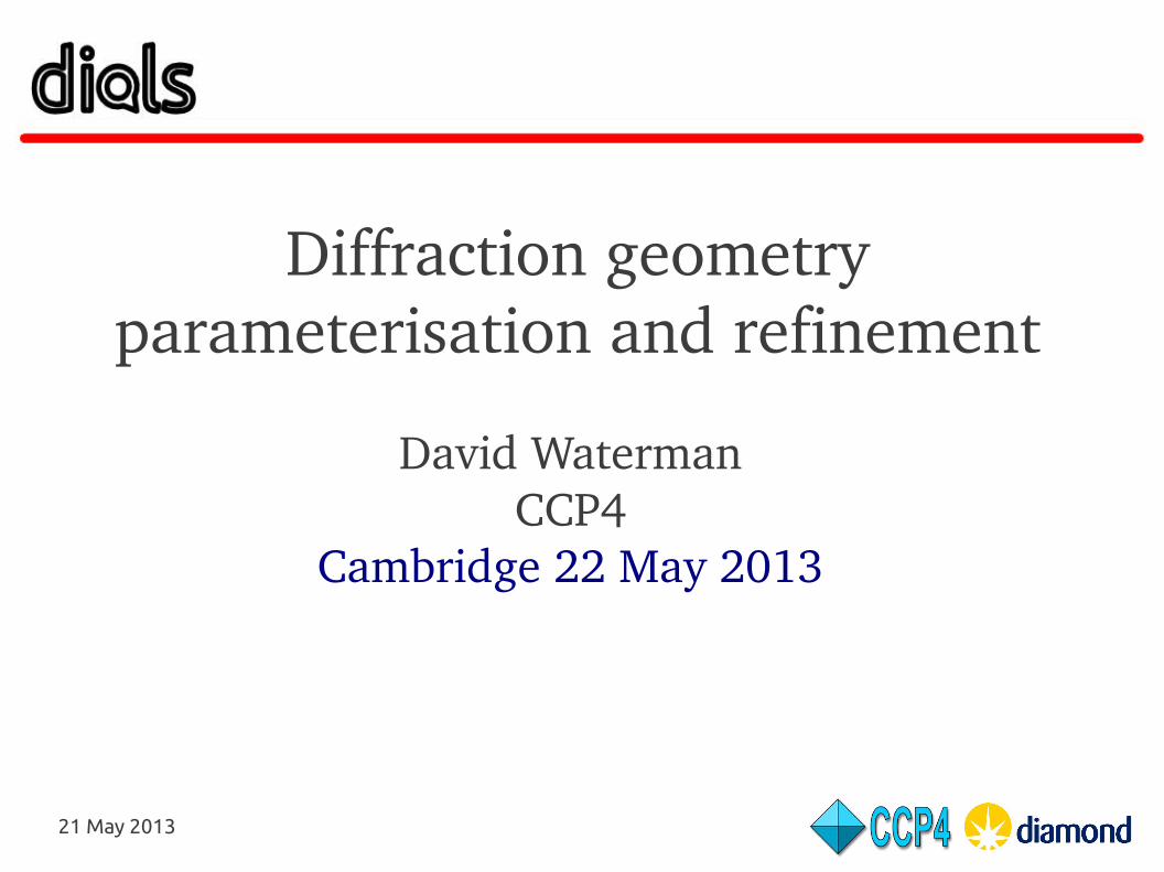
DIALS framework
21 May 2013
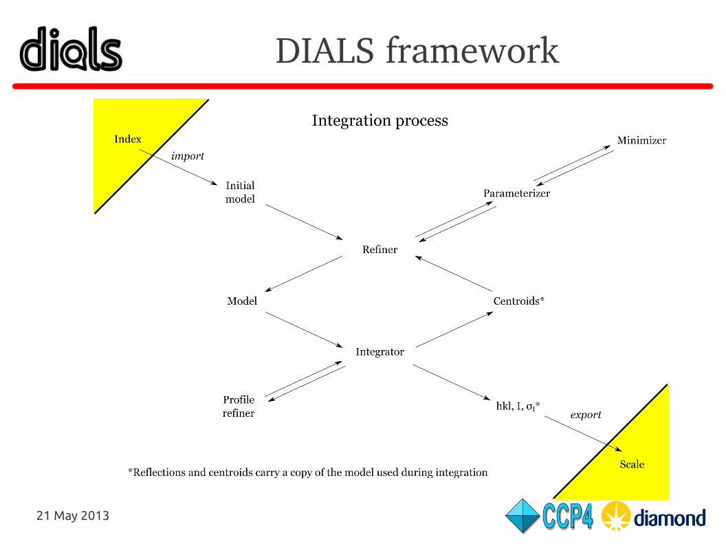
Motivation for global refinement● Input diffraction spot indices, their centroids and estimated
uncertainties (h, k, l; X, Y, ;ϕ σX, σ
Y, σ
ϕ)
● Use all (useful) data available to refine a model to reduce rmsd of predicted centroids
● Global refinement helps to recover from poorly defined parameters in local ϕ window
● More physically meaningful: avoids mopping up of effects by correlated parameters and therefore obtains realistic parameter values
● Refine profile parameters separately● Potential second round with improved centroid observations
21 May 2013
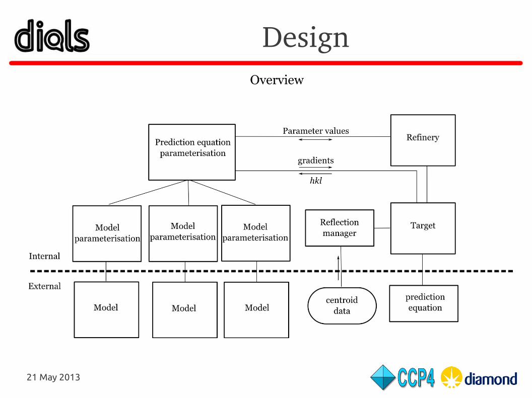
Design
21 May 2013
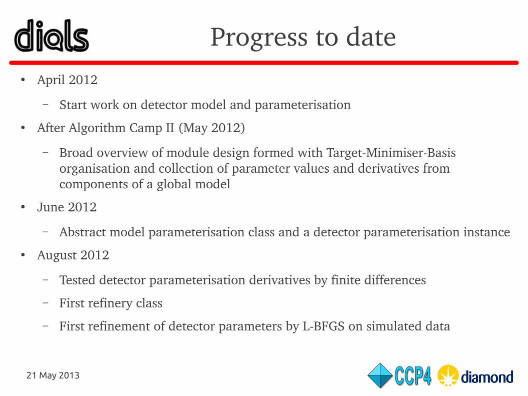
Progress to date● April 2012
– Start work on detector model and parameterisation
● After Algorithm Camp II (May 2012)
– Broad overview of module design formed with TargetMinimiserBasis organisation and collection of parameter values and derivatives from components of a global model
● June 2012
– Abstract model parameterisation class and a detector parameterisation instance
● August 2012
– Tested detector parameterisation derivatives by finite differences
– First refinery class
– First refinement of detector parameters by LBFGS on simulated data
21 May 2013
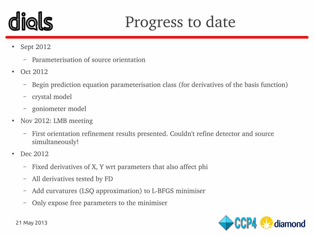
Progress to date● Sept 2012
– Parameterisation of source orientation
● Oct 2012
– Begin prediction equation parameterisation class (for derivatives of the basis function)
– crystal model
– goniometer model
● Nov 2012: LMB meeting
– First orientation refinement results presented. Couldn't refine detector and source simultaneously!
● Dec 2012
– Fixed derivatives of X, Y wrt parameters that also affect phi
– All derivatives tested by FD
– Add curvatures (LSQ approximation) to LBFGS minimiser
– Only expose free parameters to the minimiser
21 May 2013
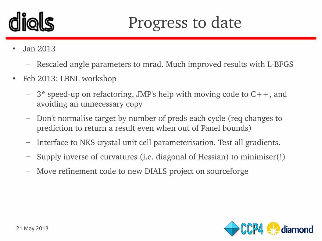
Progress to date● Jan 2013
– Rescaled angle parameters to mrad. Much improved results with LBFGS
● Feb 2013: LBNL workshop
– 3* speedup on refactoring, JMP's help with moving code to C++, and avoiding an unnecessary copy
– Don't normalise target by number of preds each cycle (req changes to prediction to return a result even when out of Panel bounds)
– Interface to NKS crystal unit cell parameterisation. Test all gradients.
– Supply inverse of curvatures (i.e. diagonal of Hessian) to minimiser(!)
– Move refinement code to new DIALS project on sourceforge
21 May 2013
Progress to date● Mar 2013
– Add LSTBX engine for nonlinear least squares refinement by GaussNewton iterations (much better)
– Convert to using new DIALS models (dxtbx) and DIALS reflection prediction throughout
● April 2013
– DIALS centroid refinement sprint. First use against real data
● May 2013
– Time dependent parameterisation of the crystal (work in progress)
21 May 2013
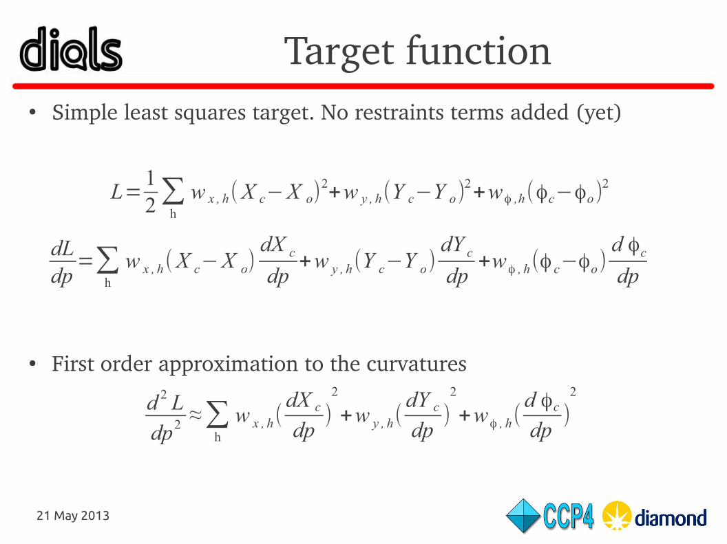
Target function● Simple least squares target. No restraints terms added (yet)
● First order approximation to the curvatures
L=12∑h
w x , h(X c−X o)2+w y , h(Y c−Y o)
2+wφ ,h(φc−φo)
2
dLdp
=∑h
w x , h(X c−X o)dX c
dp+w y , h(Y c−Y o)
dY cdp
+wφ , h(φ c−φo)d φcdp
d 2 Ldp2 ≈∑
h
w x , h(dX c
dp)
2
+w y , h(dY cdp
)2
+wφ , h(d φcdp
)2
21 May 2013
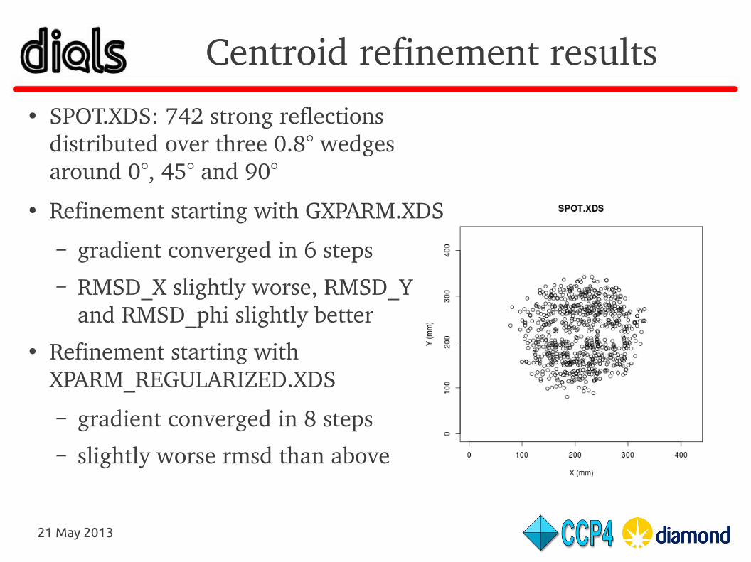
Centroid refinement results● SPOT.XDS: 742 strong reflections
distributed over three 0.8° wedges around 0°, 45° and 90°
● Refinement starting with GXPARM.XDS
– gradient converged in 6 steps– RMSD_X slightly worse, RMSD_Y
and RMSD_phi slightly better● Refinement starting with
XPARM_REGULARIZED.XDS
– gradient converged in 8 steps– slightly worse rmsd than above
21 May 2013
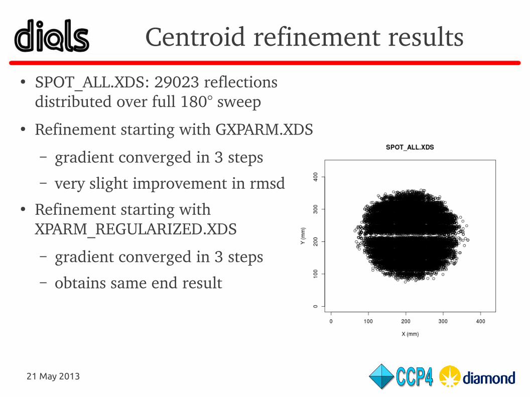
Centroid refinement results● SPOT_ALL.XDS: 29023 reflections
distributed over full 180° sweep● Refinement starting with GXPARM.XDS
– gradient converged in 3 steps– very slight improvement in rmsd
● Refinement starting with XPARM_REGULARIZED.XDS
– gradient converged in 3 steps– obtains same end result
21 May 2013
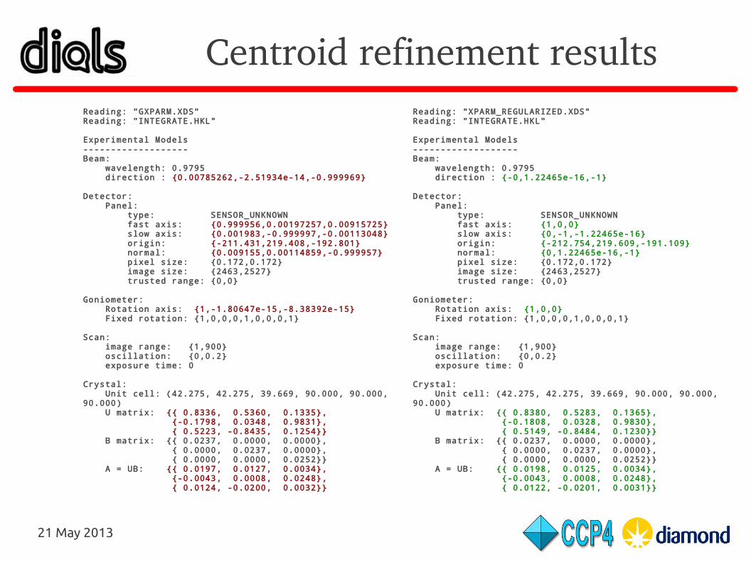
Centroid refinement resultsReading: "XPARM_REGULARIZED.XDS"Reading: "INTEGRATE.HKL"
Experimental Models-------------------Beam: wavelength: 0.9795 direction : {-0,1.22465e-16,-1}
Detector: Panel: type: SENSOR_UNKNOWN fast axis: {1,0,0} slow axis: {0,-1,-1.22465e-16} origin: {-212.754,219.609,-191.109} normal: {0,1.22465e-16,-1} pixel size: {0.172,0.172} image size: {2463,2527} trusted range: {0,0}
Goniometer: Rotation axis: {1,0,0} Fixed rotation: {1,0,0,0,1,0,0,0,1}
Scan: image range: {1,900} oscillation: {0,0.2} exposure time: 0
Crystal: Unit cell: (42.275, 42.275, 39.669, 90.000, 90.000, 90.000) U matrix: {{ 0.8380, 0.5283, 0.1365}, {-0.1808, 0.0328, 0.9830}, { 0.5149, -0.8484, 0.1230}} B matrix: {{ 0.0237, 0.0000, 0.0000}, { 0.0000, 0.0237, 0.0000}, { 0.0000, 0.0000, 0.0252}} A = UB: {{ 0.0198, 0.0125, 0.0034}, {-0.0043, 0.0008, 0.0248}, { 0.0122, -0.0201, 0.0031}}
Reading: "GXPARM.XDS"Reading: "INTEGRATE.HKL"
Experimental Models-------------------Beam: wavelength: 0.9795 direction : {0.00785262,-2.51934e-14,-0.999969}
Detector: Panel: type: SENSOR_UNKNOWN fast axis: {0.999956,0.00197257,0.00915725} slow axis: {0.001983,-0.999997,-0.00113048} origin: {-211.431,219.408,-192.801} normal: {0.009155,0.00114859,-0.999957} pixel size: {0.172,0.172} image size: {2463,2527} trusted range: {0,0}
Goniometer: Rotation axis: {1,-1.80647e-15,-8.38392e-15} Fixed rotation: {1,0,0,0,1,0,0,0,1}
Scan: image range: {1,900} oscillation: {0,0.2} exposure time: 0
Crystal: Unit cell: (42.275, 42.275, 39.669, 90.000, 90.000, 90.000) U matrix: {{ 0.8336, 0.5360, 0.1335}, {-0.1798, 0.0348, 0.9831}, { 0.5223, -0.8435, 0.1254}} B matrix: {{ 0.0237, 0.0000, 0.0000}, { 0.0000, 0.0237, 0.0000}, { 0.0000, 0.0000, 0.0252}} A = UB: {{ 0.0197, 0.0127, 0.0034}, {-0.0043, 0.0008, 0.0248}, { 0.0124, -0.0200, 0.0032}}
21 May 2013
Centroid refinement results● Refinement benefits from inclusion of more data
throughout the sweep● Need timedependent crystal model to reduce
RMSDs further● When wrong parameter fixed, crash with “Cholesky
error” nonpositivedefinite N→● Will be useful to study properties of the normal
matrix
21 May 2013
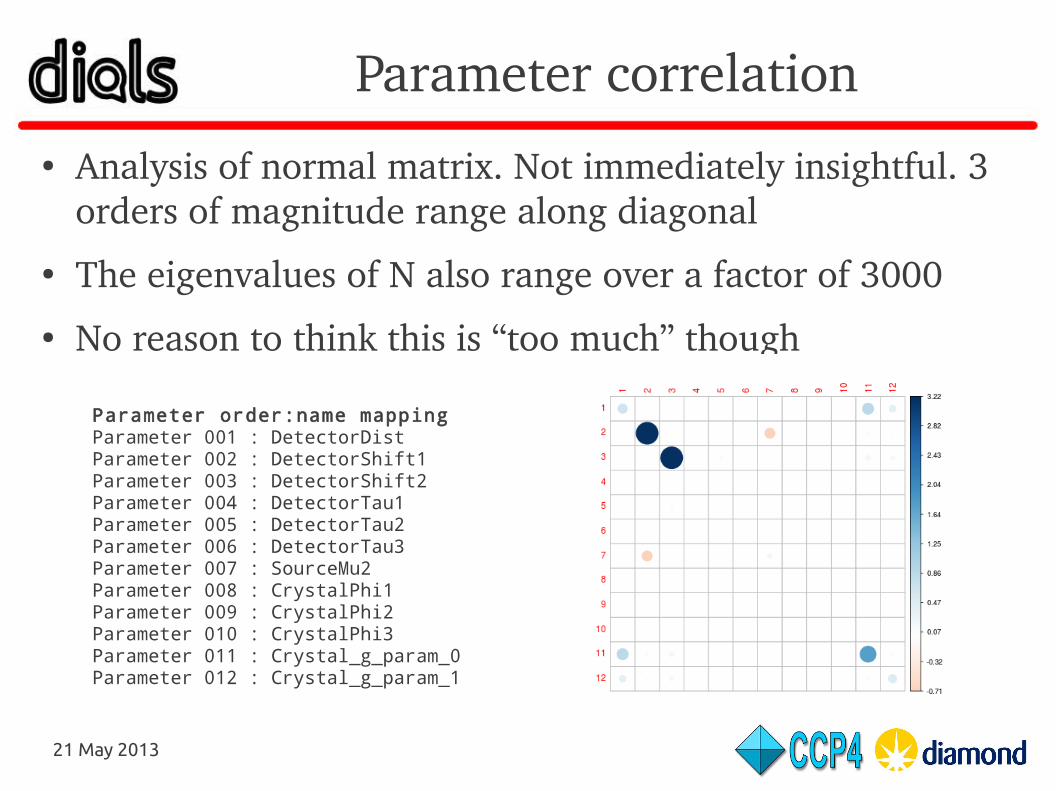
Parameter correlation● Analysis of normal matrix. Not immediately insightful. 3
orders of magnitude range along diagonal● The eigenvalues of N also range over a factor of 3000● No reason to think this is “too much” though
Parameter order:name mappingParameter 001 : DetectorDistParameter 002 : DetectorShift1Parameter 003 : DetectorShift2Parameter 004 : DetectorTau1Parameter 005 : DetectorTau2Parameter 006 : DetectorTau3Parameter 007 : SourceMu2Parameter 008 : CrystalPhi1Parameter 009 : CrystalPhi2Parameter 010 : CrystalPhi3Parameter 011 : Crystal_g_param_0Parameter 012 : Crystal_g_param_1
21 May 2013
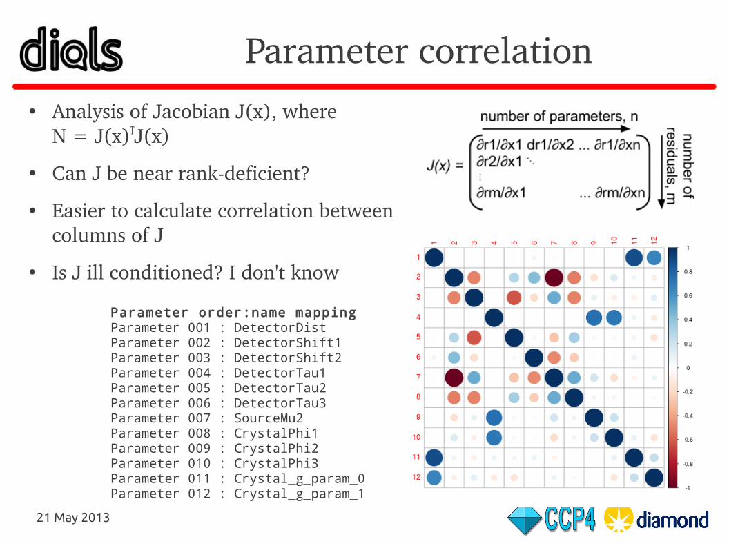
Parameter correlation● Analysis of Jacobian J(x), where
N = J(x)TJ(x)
● Can J be near rankdeficient?
● Easier to calculate correlation between columns of J
● Is J ill conditioned? I don't know
Parameter order:name mappingParameter 001 : DetectorDistParameter 002 : DetectorShift1Parameter 003 : DetectorShift2Parameter 004 : DetectorTau1Parameter 005 : DetectorTau2Parameter 006 : DetectorTau3Parameter 007 : SourceMu2Parameter 008 : CrystalPhi1Parameter 009 : CrystalPhi2Parameter 010 : CrystalPhi3Parameter 011 : Crystal_g_param_0Parameter 012 : Crystal_g_param_1
21 May 2013
Extensions to LSTBX● LSTBX solves the normal equations using the Cholesky
decomposition● This is fast, but poorly behaved when J is illconditioned
(accuracy suffers, or algorithm can even fail due to roundoff errors)
● QR is more robust, SVD even more so, at the expense of more CPU cycles
● SVD has the advantage of providing useful sensitivity information and option to filter out the smallest singular values to obtain an approximate solution less sensitive to perturbations
21 May 2013
Extensions to LSTBX● This appears closely related to the Reeke/Bricogne
“eigenvalue filtering” scheme
● What is the “best” way to solve the normal equations, perhaps admitting the possibility of filtering for correlated parameters?
● Can we get error estimates on the parameter values even in the case of filtering?
● Plan to modify LSTBX to implement a procedure for solving the normal equations that is appropriate for our circumstances
● Also try LevenbergMarquardt iterations rather than GaussNewton (already available in LSTBX) for better behaviour when J(x) is nearly rankdeficient
21 May 2013
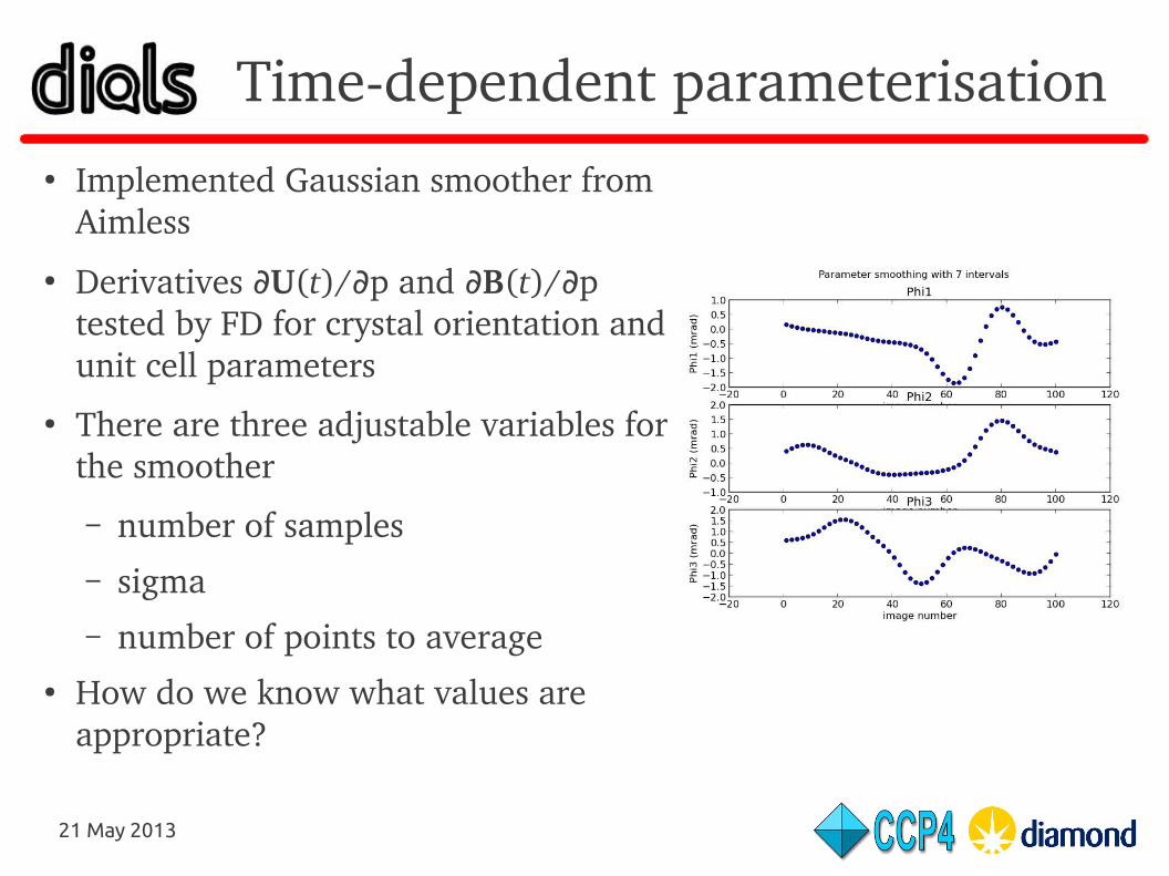
Timedependent parameterisation● Implemented Gaussian smoother from
Aimless● Derivatives ∂U(t)/ p and ∂ ∂B(t)/ p ∂
tested by FD for crystal orientation and unit cell parameters
● There are three adjustable variables for the smoother
– number of samples– sigma– number of points to average
● How do we know what values are appropriate?
21 May 2013
Timedependent parameterisation
Proposed scheme for refinement:
● A fully time invariant macrocycle to convergence to improve the detector and source models and define U
0 and B
0
● A macrocycle using timedependent crystal parameterisations and static detector and source parameterisations
– Parameters of the time dependent (Gaussian smoothed) models are restrained (tied) to the values that define U
0 and B
0
● Integration forms models for profiles, potentially improving the centroid positions
● Repeat
21 May 2013
21 May 2013
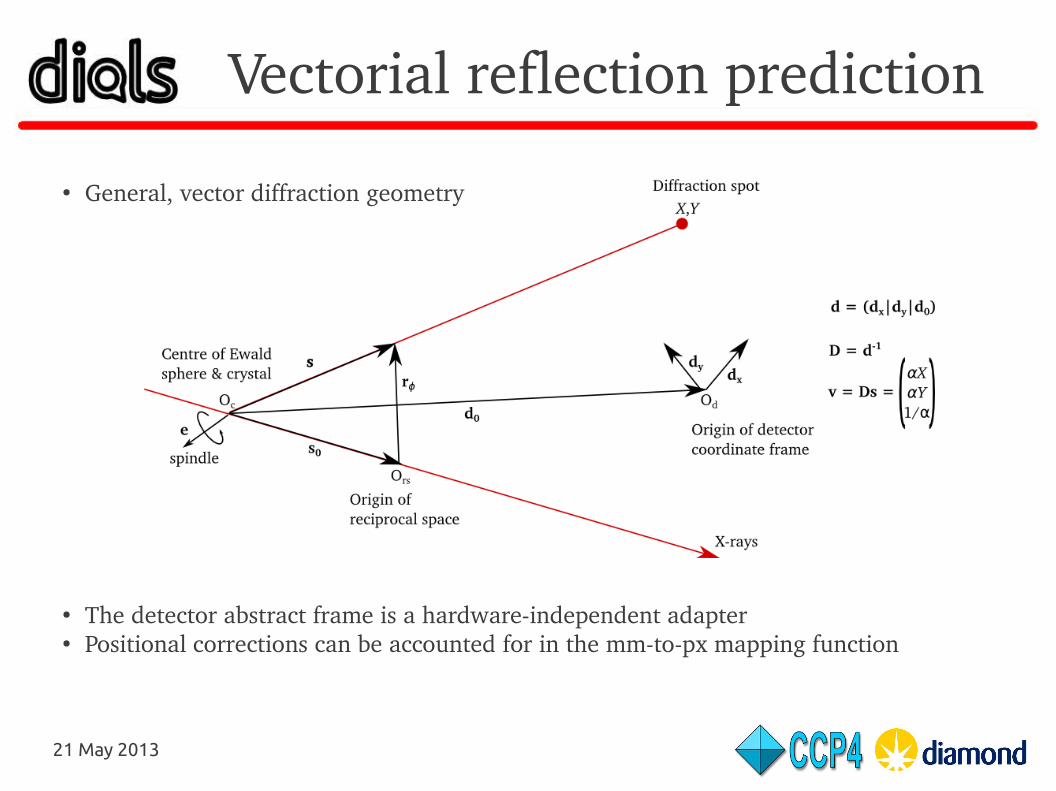
Vectorial reflection prediction
● The detector abstract frame is a hardwareindependent adapter● Positional corrections can be accounted for in the mmtopx mapping function
● General, vector diffraction geometry
21 May 2013
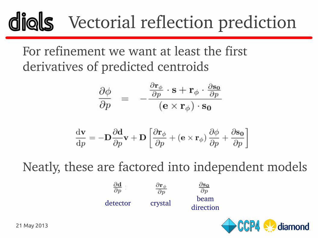
Vectorial reflection prediction
For refinement we want at least the first derivatives of predicted centroids
Neatly, these are factored into independent models
detector crystalbeam
direction
21 May 2013
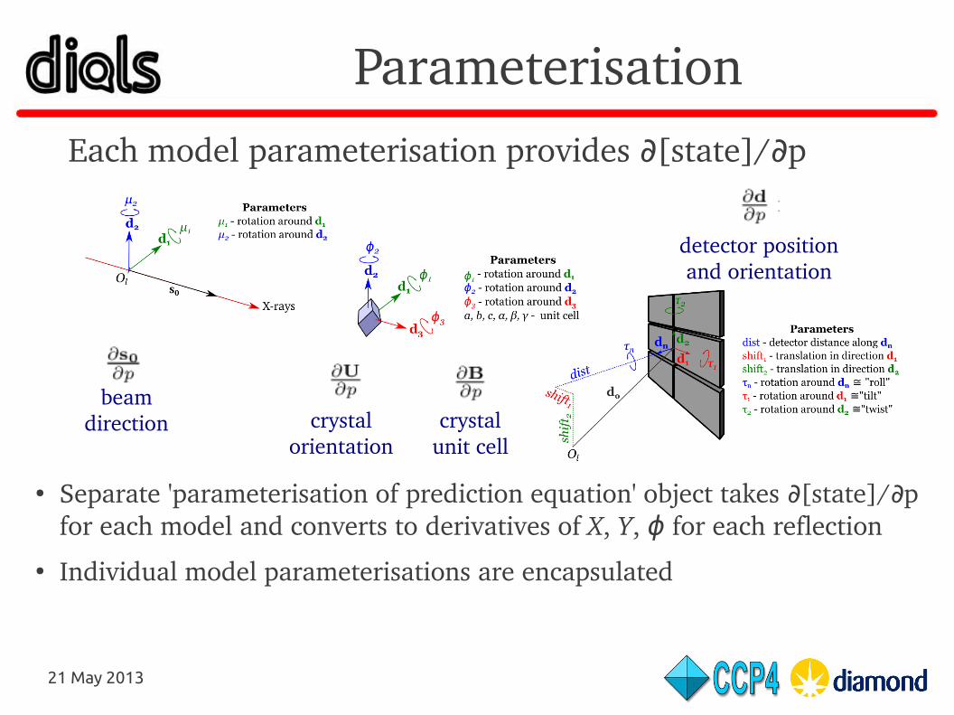
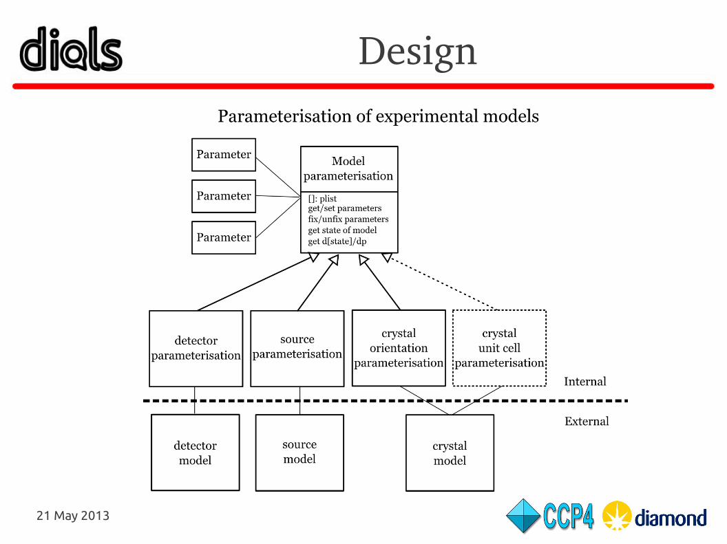
ParameterisationEach model parameterisation provides [state]/ p∂ ∂
detector positionand orientation
crystalorientation
beamdirection
● Separate 'parameterisation of prediction equation' object takes [state]/ p ∂ ∂for each model and converts to derivatives of X, Y, ϕ for each reflection
● Individual model parameterisations are encapsulated
crystalunit cell
21 May 2013
Design

21 May 2013
Parameterisation
The abstract interface specifies that:– Model parameterisations are initialised with an initial
state of the model– New states are composed by the action of functions of
the parameters on the initial state– A state and its derivatives are either a vector or a matrix– The parameters are either distances or angles with
associated unit directions
21 May 2013
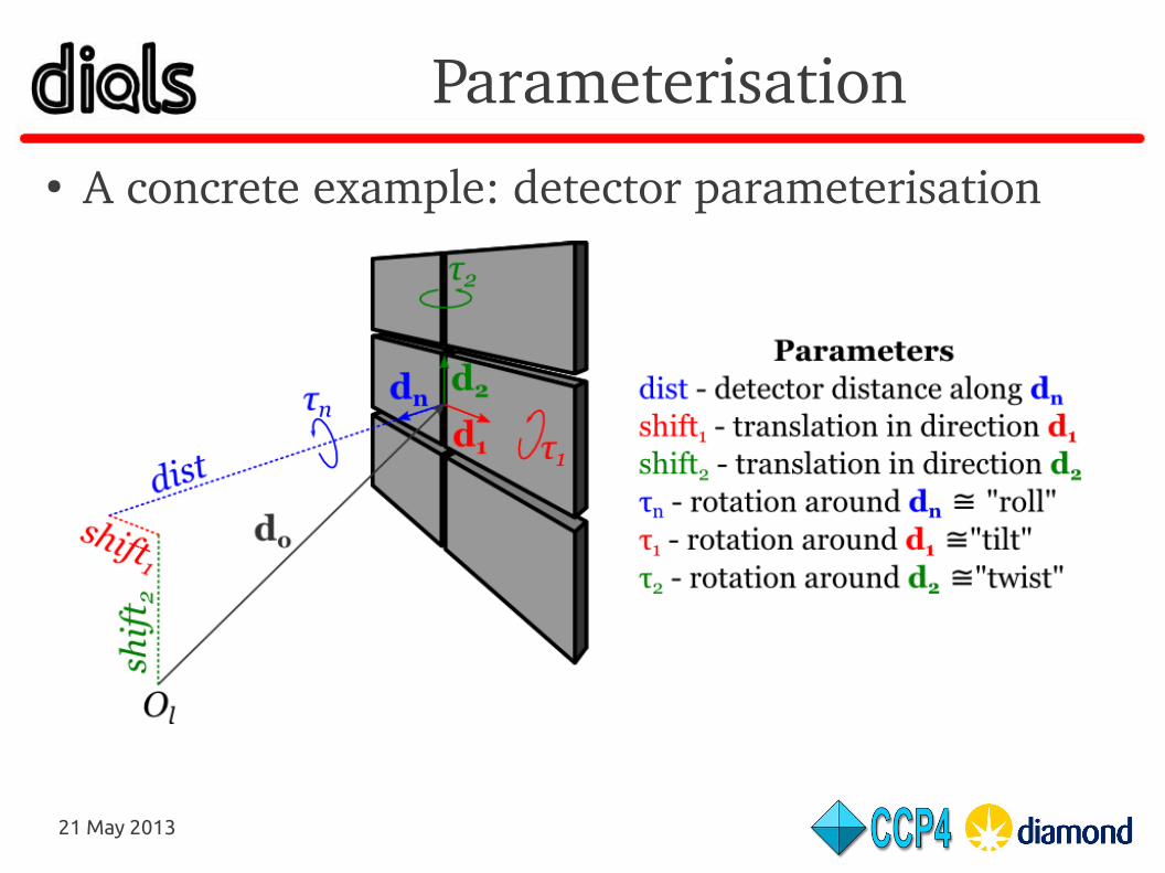
Parameterisation● A concrete example: detector parameterisation
21 May 2013
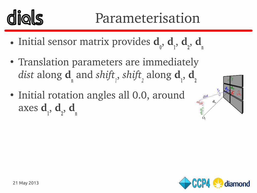
Parameterisation● Initial sensor matrix provides d
0, d
1, d
2, d
n
● Translation parameters are immediately dist along d
n and shift
1, shift
2 along d
1, d
2
● Initial rotation angles all 0.0, around axes d
1, d
2, d
n
21 May 2013
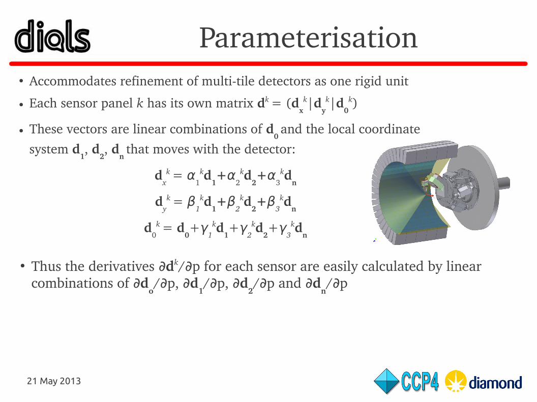
Parameterisation● Accommodates refinement of multitile detectors as one rigid unit
● Each sensor panel k has its own matrix dk = (dxk|d
yk|d
0k)
● These vectors are linear combinations of d0 and the local coordinate
system d1, d
2, d
n that moves with the detector:
dxk = α
1kd
1+α
2kd
2+α
3kd
n
dyk = β
1kd
1+β
2kd
2+β
3kd
n
d0k = d
0+γ
1kd
1+γ
2kd
2+γ
3kd
n
● Thus the derivatives ∂dk/ p for each sensor are easily calculated by linear ∂combinations of ∂d
o/ p, ∂ ∂d
1/ p, ∂ ∂d
2/ p and ∂ ∂d
n/ p∂
21 May 2013
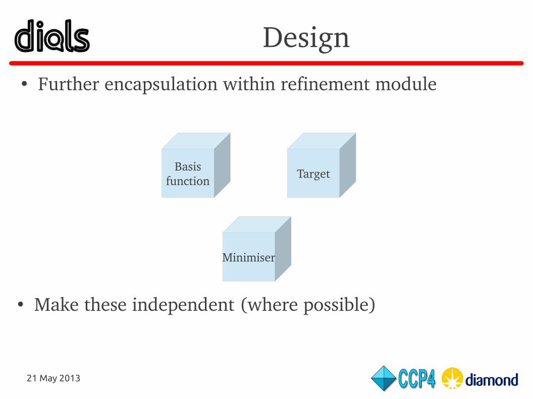
Design● Further encapsulation within refinement module
● Make these independent (where possible)
Minimiser
TargetBasis
function