Embed Size (px)
Citation preview
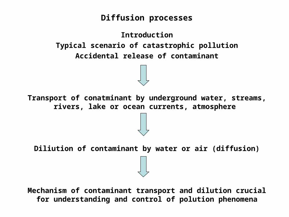
Diffusion processes
Introduction
Typical scenario of catastrophic pollution
Accidental release of contaminant
Transport of conatminant by underground water, streams, rivers, lake or ocean currents, atmosphere
Diliution of contaminant by water or air (diffusion)
Mechanism of contaminant transport and dilution crucial for understanding and control of polution phenomena
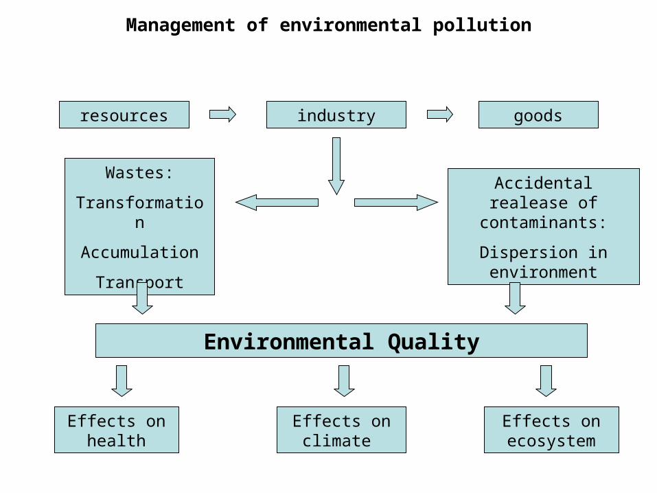
Management of environmental pollution
resources industry goods
Wastes:
Transformation
Accumulation
Transport
Accidental realease of contaminants:
Dispersion in environment
Environmental Quality
Effects on health
Effects on climate
Effects on ecosystem
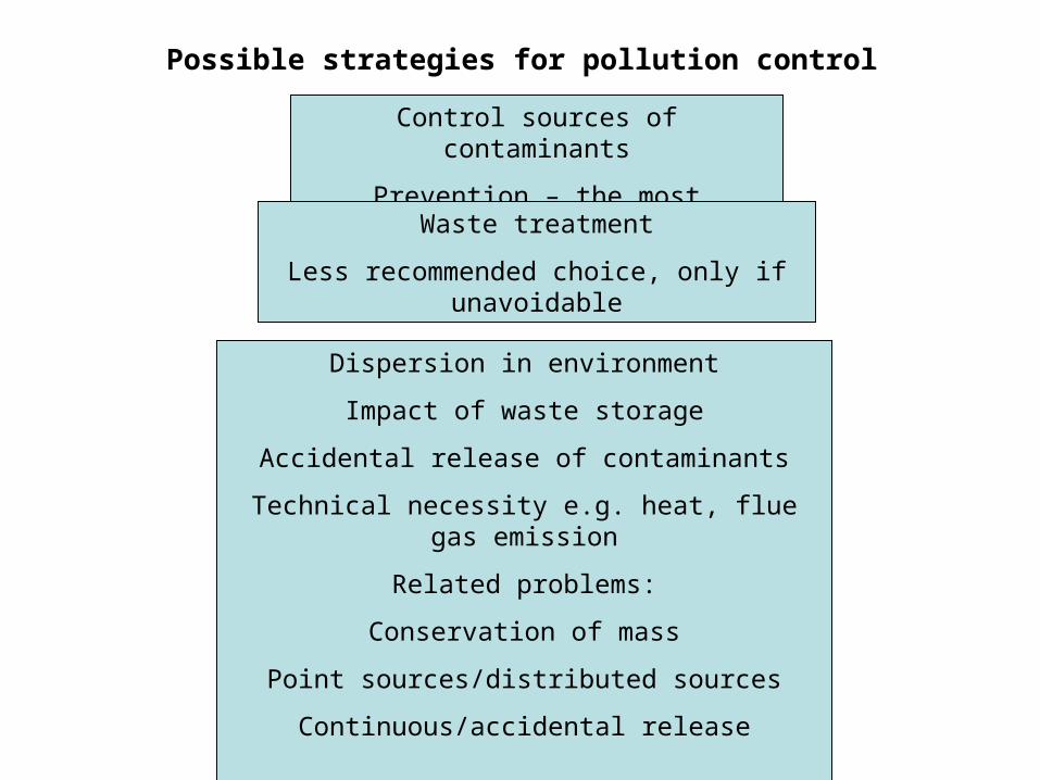
Possible strategies for pollution control
Control sources of contaminants
Prevention – the most recommended
Waste treatment
Less recommended choice, only if unavoidable
Dispersion in environment
Impact of waste storage
Accidental release of contaminants
Technical necessity e.g. heat, flue gas emission
Related problems:
Conservation of mass
Point sources/distributed sources
Continuous/accidental release
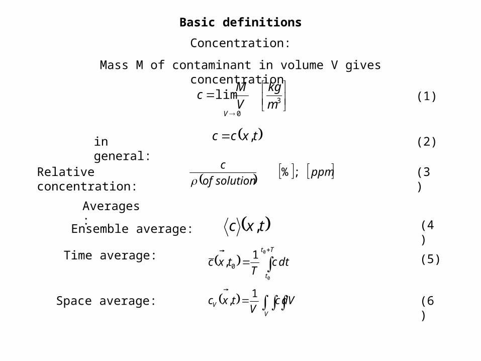
Basic definitions
3
0
limm
kg
V
Mc
V
txcc ,
ppmsolutionof
c;%
Concentration:
Mass M of contaminant in volume V gives concentration
(1)
in general: (2)
Relative concentration: (3)
Averages:
Ensemble average: txc ,
Time average:
Tt
t
dtcT
txc0
0
1, 0
Space average: V
V dVcV
txc1
,
(4)
(5)
(6)
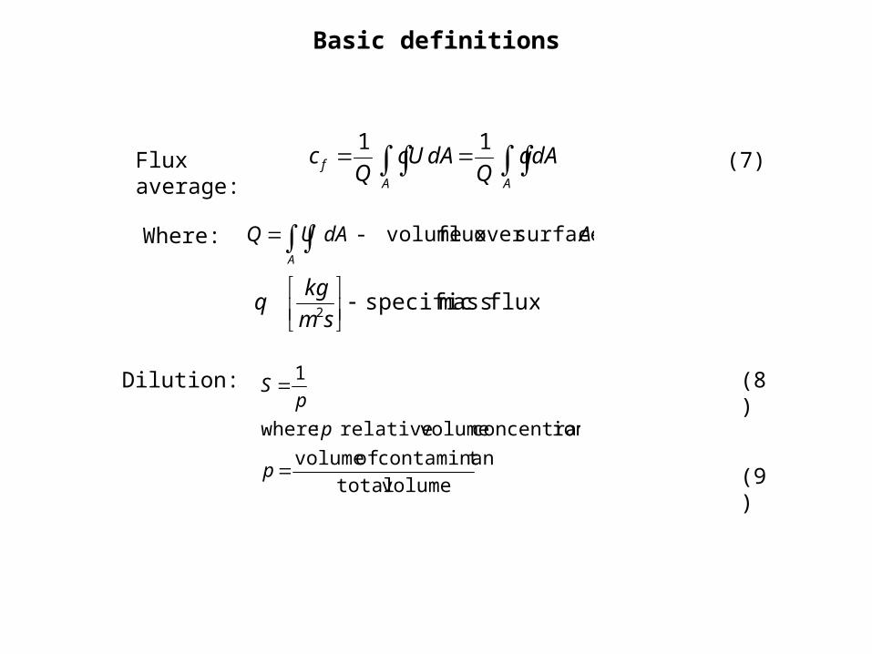
Basic definitions
AA
f dAqQ
dAcUQ
c11
AdAUQA
surfaceover flux volume-
flux mass specific 2
sm
kgq
Flux average: (7)
Where:
Dilution:
volumetotal
tcontaminan of volume
ionconcentrat volumerelative :where
1
p
p
pS (8)
(9)
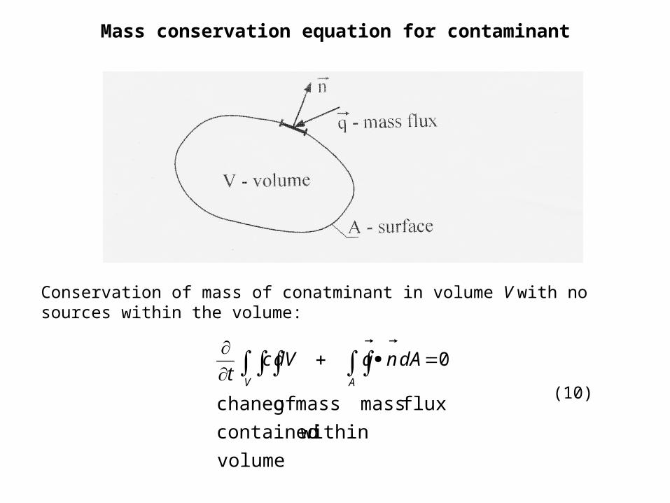
Mass conservation equation for contaminant
Conservation of mass of conatminant in volume V with no sources within the volume:
volume
withincontained
flux mass mass of chaneg
0
dAnqdVct AV
(10)

Mass conservation equation for contaminant
Due to Gauss-Ostrogradski transformation
0
dVqxt
c
V
ii
0
ii
qxt
c
diffusion advection Diii qcUq
(11)
Since V is an arbitrary volume:
(12)
Flux of contaminant:
(13)
Substitution of Eq.(13) into Eq. (12) leads to
Dii
ii
qx
cUxt
c
(14)
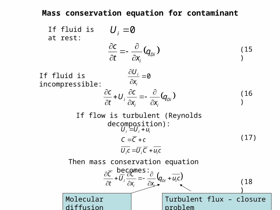
Mass conservation equation for contaminant
0iU
Dii
qxt
c
0
i
i
x
U
If fluid is at rest:
(15)
If fluid is incompressible:
Diii
i qxx
cU
t
c
If flow is turbulent (Reynolds decomposition):
cuCUcU
cCC
uUU
iii
iii
Then mass conservation equation becomes:
cuqxx
CU
t
CiDi
iii
(16)
Molecular diffusion Turbulent flux – closure problem
(17)
(18)
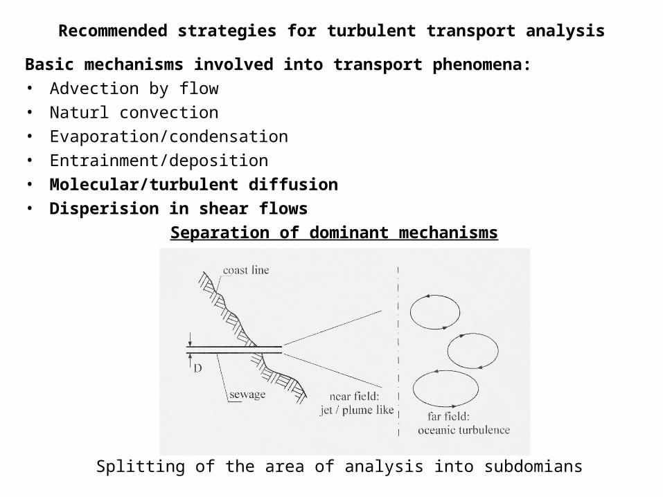
Recommended strategies for turbulent transport analysis
Basic mechanisms involved into transport phenomena:
• Advection by flow
• Naturl convection
• Evaporation/condensation
• Entrainment/deposition
• Molecular/turbulent diffusion
• Disperision in shear flows
Separation of dominant mechanisms
Splitting of the area of analysis into subdomians
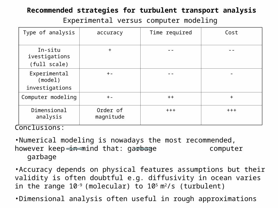
Recommended strategies for turbulent transport analysis
Experimental versus computer modeling
Type of analysis accuracy Time required Cost
In-situ ivestigations
(full scale)
+ -- --
Experimental (model)
investigations
+- -- -
Computer modeling +- ++ +
Dimensional analysis Order of magnitude +++ +++
Conclusions:
•Numerical modeling is nowadays the most recommended, however keep in mind that: garbage computer garbage
•Accuracy depends on physical features assumptions but their validity is often doubtful e.g. diffusivity in ocean varies in the range 10-9 (molecular) to 105 m2/s (turbulent)
•Dimensional analysis often useful in rough approximations
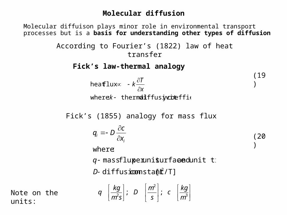
Molecular diffusion
Molecular diffuison plays minor role in environmental transport processes but is a basis for understanding other types of diffusion
coeffienty diffusivit thermal :where
flux heat
kx
Tk
Fick’s law-thermal analogy
According to Fourier’s (1822) law of heat transfer
(19)
Fick’s (1855) analogy for mass flux
/T][Lconstant diffusion
unit time and surfaceunit per flux mass
:where
2D-
q
x
cDq
ii
(20)
Note on the units:
3
2
2;;
m
kgc
s
mD
sm
kgq
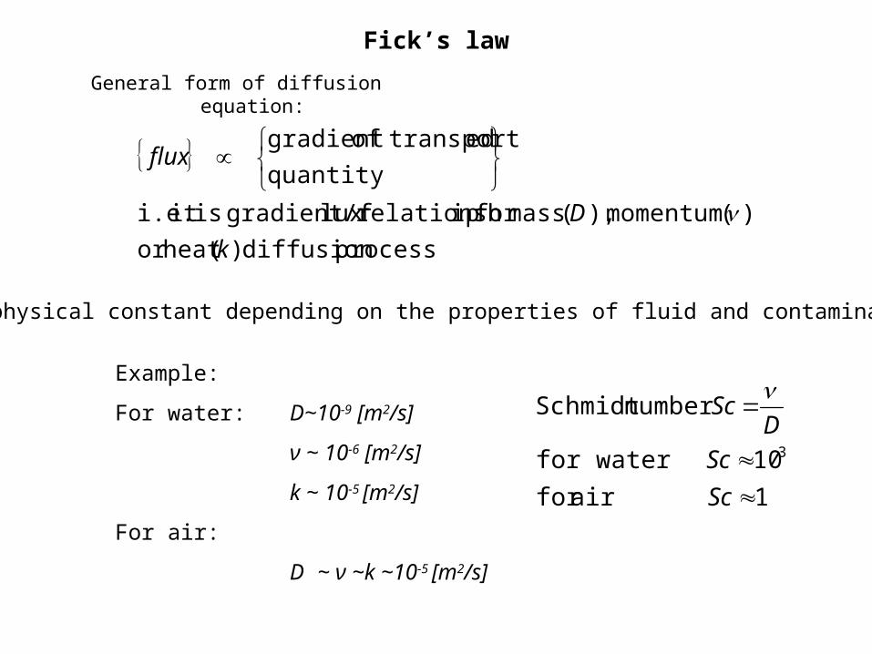
Fick’s law
General form of diffusion equation:
processdiffusion )(heat or
)( momentum ),( massfor iprelationshlux gradient/f isit i.e.
quantity
ed transportofgradient
k
D
flux
D - physical constant depending on the properties of fluid and contaminant
Example:
For water: D~10-9 [m2/s]
ν ~ 10-6 [m2/s]
k ~ 10-5 [m2/s]
For air:
D ~ ν ~k ~10-5 [m2/s]
1 air for
10 for water
number Schmidt
3
Sc
Sc
DSc
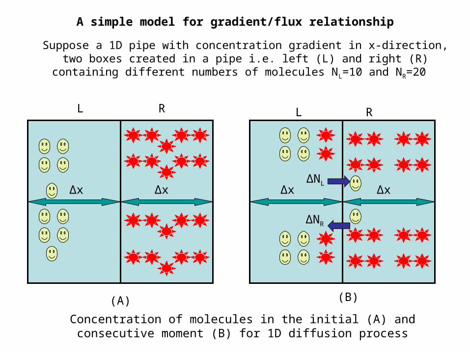
A simple model for gradient/flux relationship
Suppose a 1D pipe with concentration gradient in x-direction, two boxes created in a pipe i.e. left (L) and right (R) containing different numbers of
molecules NL=10 and NR=20
L R
Δx Δx Δx Δx
LR
(A) (B)
Concentration of molecules in the initial (A) and consecutive moment (B) for 1D diffusion process
ΔNL
ΔNR
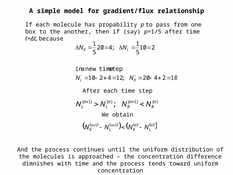
A simple model for gradient/flux relationship
182420;124210
step timenew ain
2105
1;420
5
1
RL
LR
NN
NN
)()1()()1( ; nR
nR
nL
nL NNNN
If each molecule has propability p to pass from one box to the another, then if (say) p=1/5 after time t+Δt, because
After each time step
We obtain
nL
nR
nL
nR NNNN 11
And the process continues until the uniform distribution of the molecules is approached – the concentration difference dimnishes with time and the process
tends toward uniform concentration
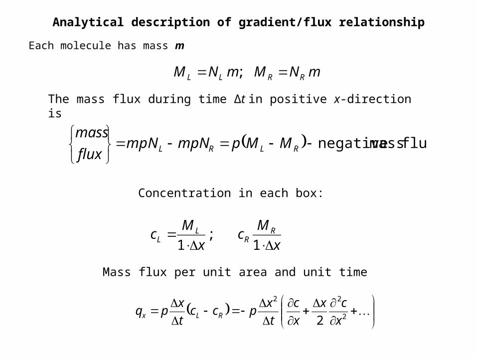
Analytical description of gradient/flux relationship
Each molecule has mass m
mNMmNM RRLL ;
The mass flux during time Δt in positive x-direction is
flux mass negative
RLRL MMppNmNpmflux
mass
Concentration in each box:
x
Mc
x
Mc R
RL
L
1;
1
Mass flux per unit area and unit time
2
22
2 x
cx
x
c
t
xpcc
t
xpq RLx
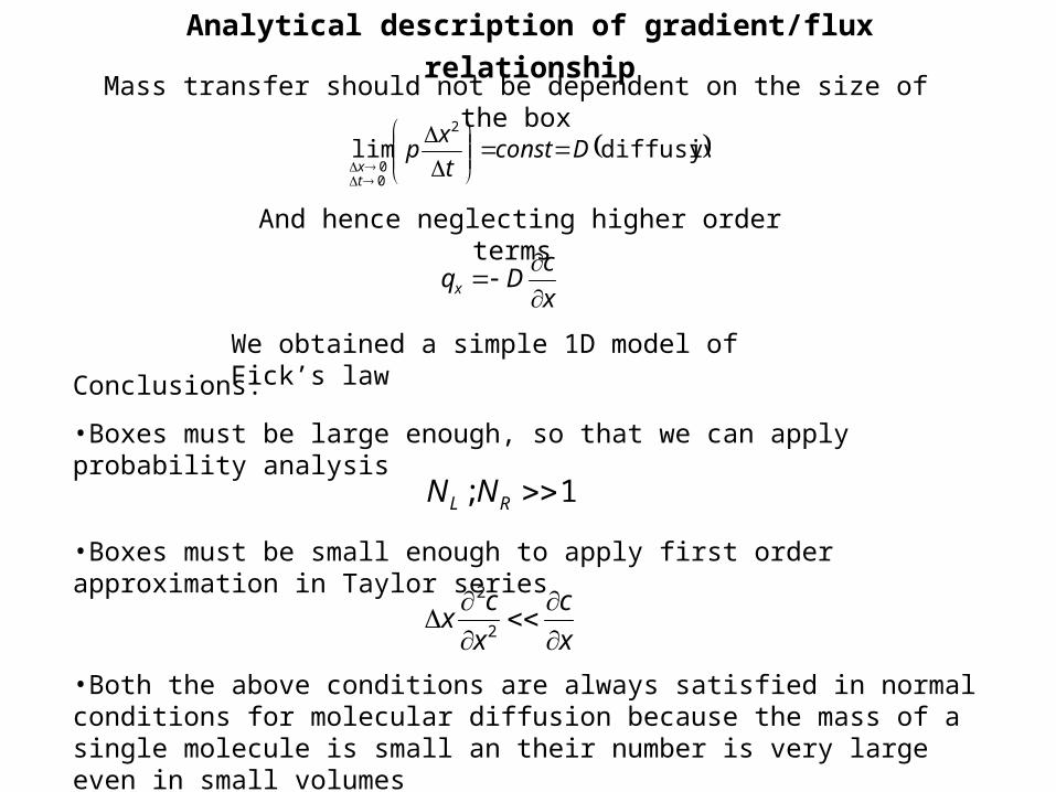
Analytical description of gradient/flux relationship
ydiffusivitlim2
00
Dconstt
xp
tx
x
cDqx
1; RL NN
Mass transfer should not be dependent on the size of the box
And hence neglecting higher order terms
We obtained a simple 1D model of Fick’s law
Conclusions:
•Boxes must be large enough, so that we can apply probability analysis
•Boxes must be small enough to apply first order approximation in Taylor series
x
c
x
cx
2
2
•Both the above conditions are always satisfied in normal conditions for molecular diffusion because the mass of a single molecule is small an their number is very large even in small volumes
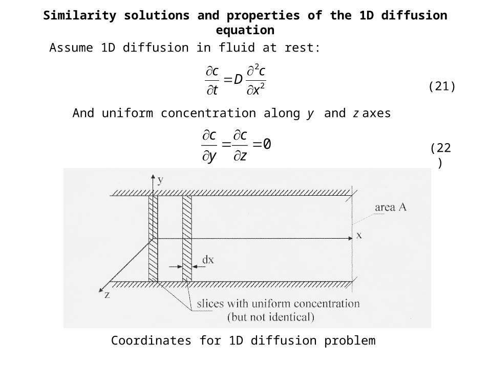
Similarity solutions and properties of the 1D diffusion equation
2
2
x
cD
t
c
Assume 1D diffusion in fluid at rest:
(21)
And uniform concentration along y and z axes
0
z
c
y
c(22)
Coordinates for 1D diffusion problem
Similarity solutions and properties of the 1D diffusion equation
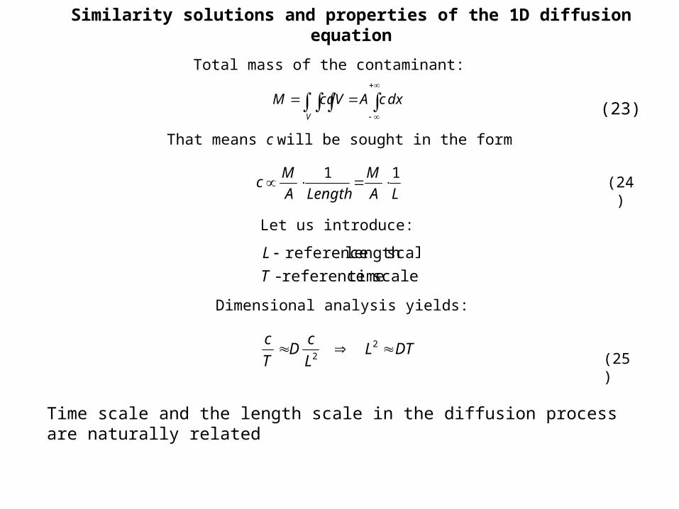
Total mass of the contaminant:
V
dxcAdVcM
LA
M
LengthA
Mc
11
scale timereference -
scalelength reference
T
L
(23)
That means c will be sought in the form
(24)
Let us introduce:
Dimensional analysis yields:
DTLL
cD
T
c 2
2 (25)
Time scale and the length scale in the diffusion process are naturally related
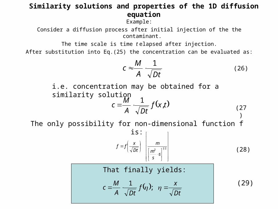
Example:
Consider a diffusion process after initial injection of the the contaminant.
The time scale is time t elapsed after injection.
After substitution into Eq.(25) the concentration can be evaluated as:
DtA
Mc
1
Similarity solutions and properties of the 1D diffusion equation
(26)
i.e. concentration may be obtained for a similarity solution
txfDtA
Mc ,
1
The only possibility for non-dimensional function f is:
(27)
212
ss
m
m
Dt
xff
(28)
That finally yields:
Dt
xf
DtA
Mc ;
1 (29)
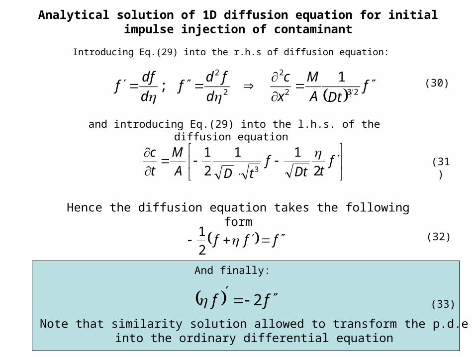
Analytical solution of 1D diffusion equation for initial impulse injection of contaminant
Introducing Eq.(29) into the r.h.s of diffusion equation:
f
DtA
M
x
c
d
fdf
d
dff
232
2
2
2 1;
(30)
and introducing Eq.(29) into the l.h.s. of the diffusion equation
ftDt
ftDA
M
t
c
2
11
2
13
(31)
Hence the diffusion equation takes the following form
fff 2
1 (32)
And finally:
ff 2 (33)
Note that similarity solution allowed to transform the p.d.e into the ordinary differential equation
Analytical solution of 1D diffusion equation for initial impulse injection of contaminant
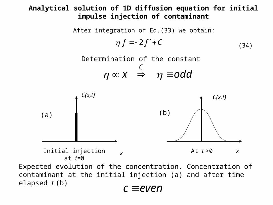
After integration of Eq.(33) we obtain:
Cff 2
oddx
(34)
Determination of the constant C
Expected evolution of the concentration. Concentration of contaminant at the initial injection (a) and after time elapsed t (b)
C(x,t) C(x,t)
x xInitial injection at t=0 At t >0
(a) (b)
evenc
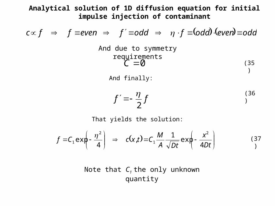
Analytical solution of 1D diffusion equation for initial impulse injection of contaminant
oddevenoddfoddfevenffc
0C
ff2
And due to symmetry requirements
(35)
And finally:
(36)
That yields the solution:
Dt
x
DtA
MCtxcCf
4exp
1,
4exp
2
1
2
1
(37)
Note that C1 the only unknown quantity
14
exp2
1
Dt
dx
Dt
xC
a
dxxa
22exp
41
1 C
Analytical solution of 1D diffusion equation for initial impulse injection of contaminant
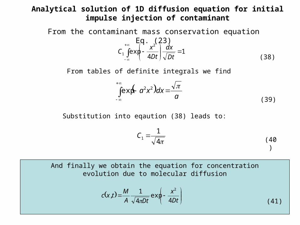
From the contaminant mass conservation equation Eq. (23)
(38)
From tables of definite integrals we find
(39)
Substitution into eqaution (38) leads to:
(40)
And finally we obtain the equation for concentration evolution due to molecular diffusion
Dt
x
DtA
Mtxc
4exp
4
1,
2
(41)
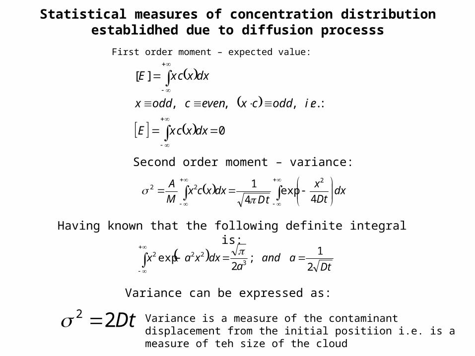
Statistical measures of concentration distribution establidhed due to diffusion processs
First order moment – expected value:
0
:..,,,
][
dxxcxE
eioddcxevencoddx
dxxcxE
Second order moment – variance:
dx
Dt
x
tDdxxcx
M
A
4exp
4
1 222
Having known that the following definite integral is:
Dt
aanda
dxxax2
1;
2exp
3222
Variance can be expressed as:
Dt22 Variance is a measure of the contaminant displacement from the initial positiion i.e. is a measure of teh size of the cloud
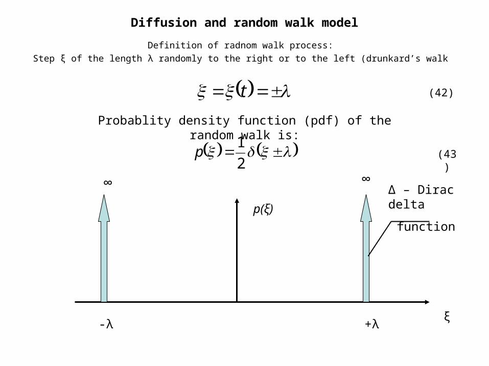
Diffusion and random walk model
Definition of radnom walk process:
Step ξ of the length λ randomly to the right or to the left (drunkard’s walk
t (42)
Probablity density function (pdf) of the random walk is:
2
1p
+λ-λ
∞ ∞Δ – Dirac delta
function
ξ
p(ξ)
(43)
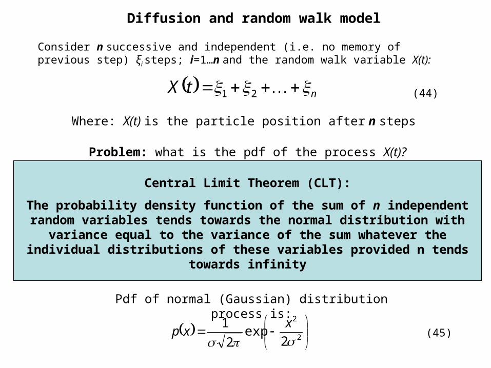
Diffusion and random walk model
Consider n successive and independent (i.e. no memory of previous step) ξi steps; i=1…n and the random walk variable X(t):
ntX 21 (44)
Where: X(t) is the particle position after n steps
Problem: what is the pdf of the process X(t)?
Central Limit Theorem (CLT):
The probability density function of the sum of n independent random variables tends towards the normal distribution with variance equal to the
variance of the sum whatever the individual distributions of these variables provided n tends towards infinity
Pdf of normal (Gaussian) distribution process is:
2
2
2exp
2
1
x
xp (45)
Diffusion and random walk model
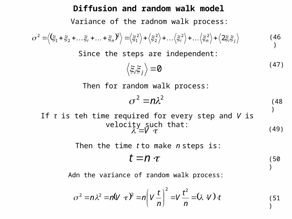
Variance of the radnom walk process:
jinini 22222
21
221
2
0ji
22 n
(46)
Since the steps are independent:
(47)
Then for random walk process:
(48)
If τ is teh time required for every step and V is velocity such that:
V (49)
Then the time t to make n steps is:
nt
Adn the variance of random walk process:
(50)
tVn
tV
n
tVnVnn
22222
(51)

Diffusion and random walk model
tV 2 (52)
Close analogy of random walk process to molecular diffusion with λ analogous to mean free path and V analogous to molecular agitation (≈ temperature), which finally leads to the expression for diffusivity:
DV (53)
Example: N molecules of mass m injected into infinitely thin layer
Diffusion and random walk model
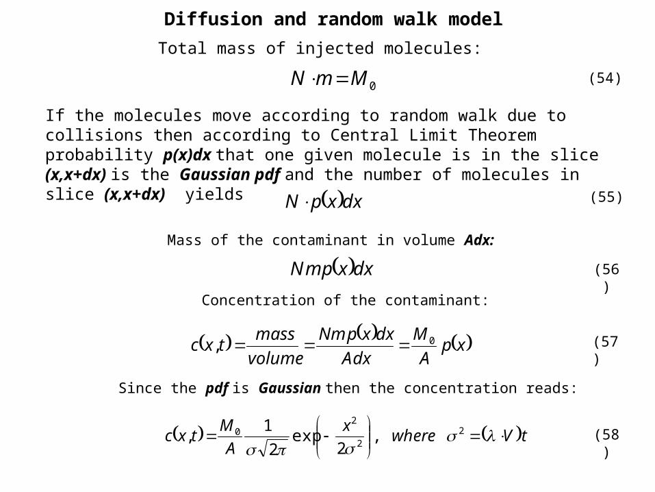
Total mass of injected molecules:
0MmN
dxxpN
dxxpmN
(54)
If the molecules move according to random walk due to collisions then according to Central Limit Theorem probability p(x)dx that one given molecule is in the slice (x,x+dx) is the Gaussian pdf and the number of molecules in slice (x,x+dx) yields
(55)
Mass of the contaminant in volume Adx:
Concentration of the contaminant:
xpA
M
dxA
dxxpNm
volume
masstxc 0,
Since the pdf is Gaussian then the concentration reads:
(56)
(57)
(58) tVwherex
A
Mtxc
2
2
20 ,
2exp
2
1,
Diffusion and random walk model
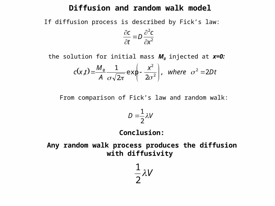
If diffusion process is described by Fick’s law:
2
2
x
cD
t
c
tDwherex
A
Mtxc 2,
2exp
2
1, 2
2
20
the solution for initial mass M0 injected at x=0:
From comparison of Fick’s law and random walk:
VD 2
1
Conclusion:
Any random walk process produces the diffusion with diffusivity
V2
1
Diffusion and random walk model
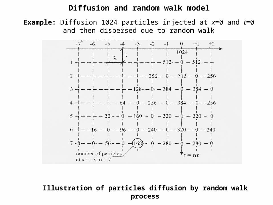
Example: Diffusion 1024 particles injected at x=0 and t=0 and then dispersed due to random walk
Illustration of particles diffusion by random walk process
Diffusion and random walk model
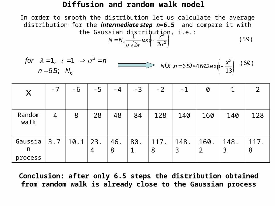
In order to smooth the distribution let us calculate the average distribution for the intermediate step n=6.5 and compare it with the Gaussian distribution, i.e.:
2
2
0 2exp
2
1
x
NN
0
2
;5.6
1,1
Nn
nfor
13exp2.1605.6,
2xnXN
(59)
(60)
x -7 -6 -5 -4 -3 -2 -1 0 1 2
Random walk
4 8 28 48 84 128 140 160 140 128
Gaussian
process3.7 10.1 23.4 46.8 80.1 117.8 148.3 160.2 148.3 117.8
Conclusion: after only 6.5 steps the distribution obtained from random walk is already close to the Gaussian process
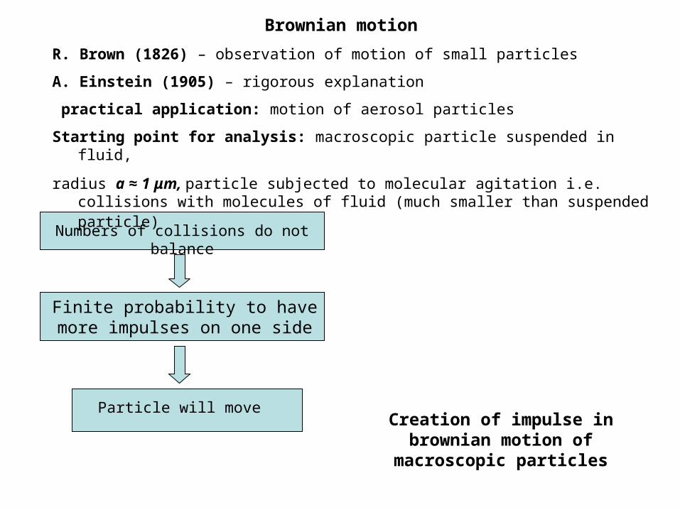
Brownian motion
R. Brown (1826) – observation of motion of small particles
A. Einstein (1905) – rigorous explanation
practical application: motion of aerosol particles
Starting point for analysis: macroscopic particle suspended in fluid,
radius a ≈ 1 μm, particle subjected to molecular agitation i.e. collisions with molecules of fluid (much smaller than suspended particle)
Numbers of collisions do not balance
Finite probability to have more impulses on one side
Particle will moveCreation of impulse in brownian motion of macroscopic particles
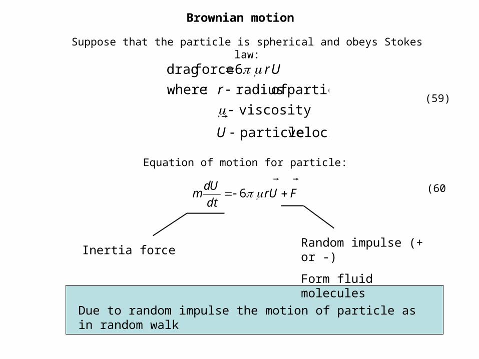
Brownian motion
Suppose that the particle is spherical and obeys Stokes law:
velocityparticle
viscosity
particle of radius:where
6forcedrag
U
r
Ur
(59)
Equation of motion for particle:
FUrdt
Udm
6 (60
Inertia forceRandom impulse (+ or -)
Form fluid molecules
Due to random impulse the motion of particle as in random walk
Brownian motion
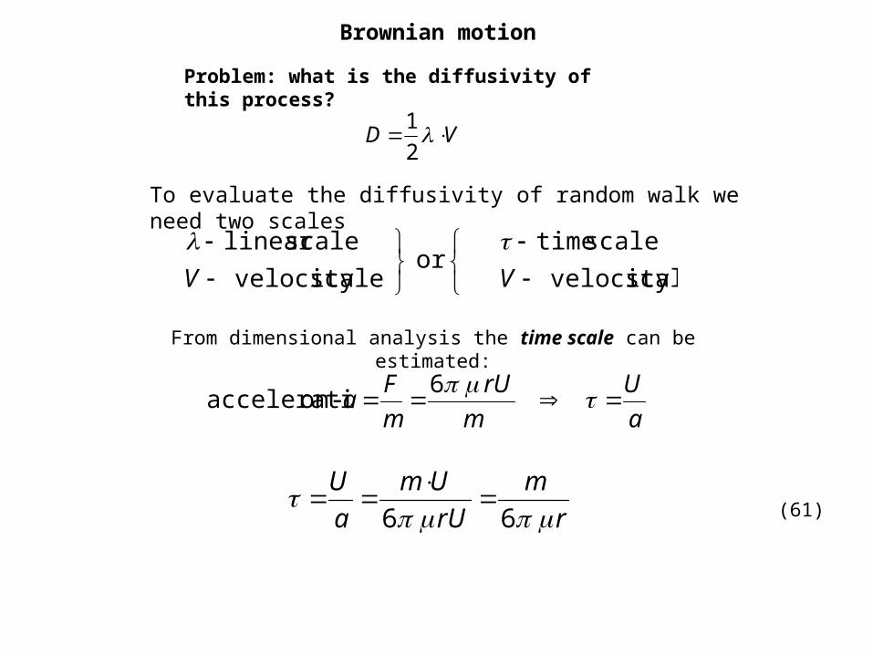
Problem: what is the diffusivity of this process?
VD 2
1
scale velocity
scale time or
scale velocity
scalelinear
VV
r
m
rU
Um
a
U
66
To evaluate the diffusivity of random walk we need two scales
From dimensional analysis the time scale can be estimated:
a
U
m
Ur
m
Fa 6 -on accelerati
(61)
Brownian motion
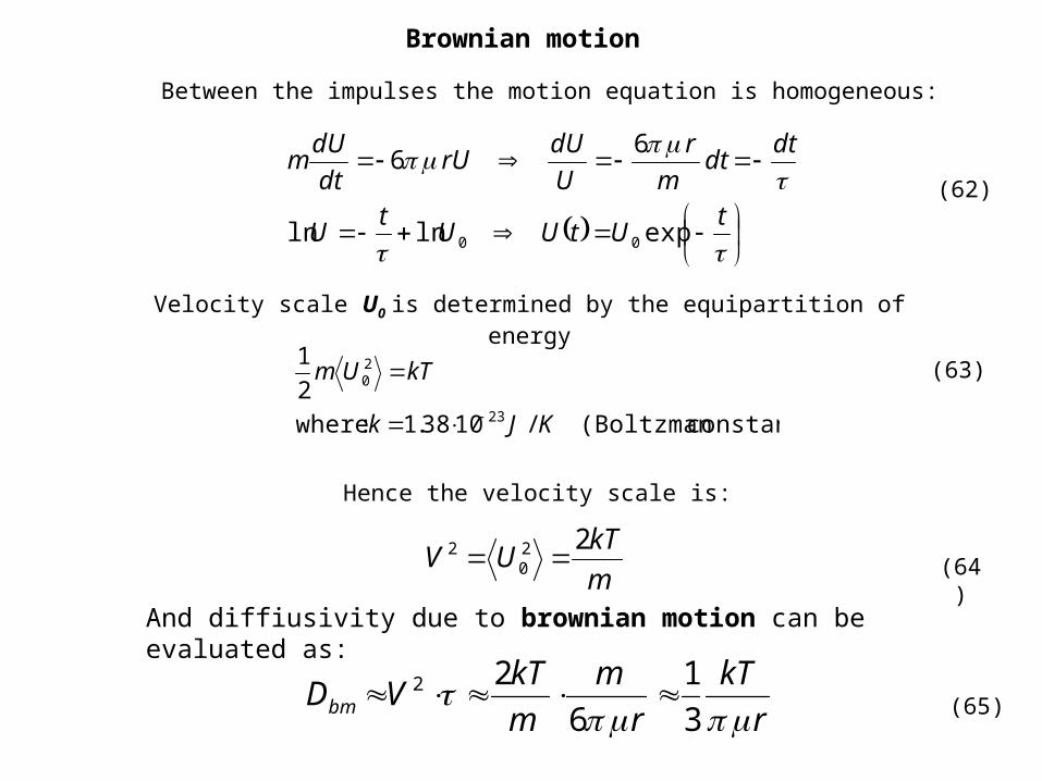
Between the impulses the motion equation is homogeneous:
tUtUU
tU
dtdt
m
r
U
dUUr
dt
dUm
explnln
66
00
constant)(Boltzman /1038.1 :where
2
1
23
20
KJk
TkUm
m
kTUV
220
2
(62)
Velocity scale U0 is determined by the equipartition of energy
(63)
Hence the velocity scale is:
(64)
And diffiusivity due to brownian motion can be evaluated as:
r
kT
r
m
m
kTVDbm
3
1
6
22 (65)
Brownian motion
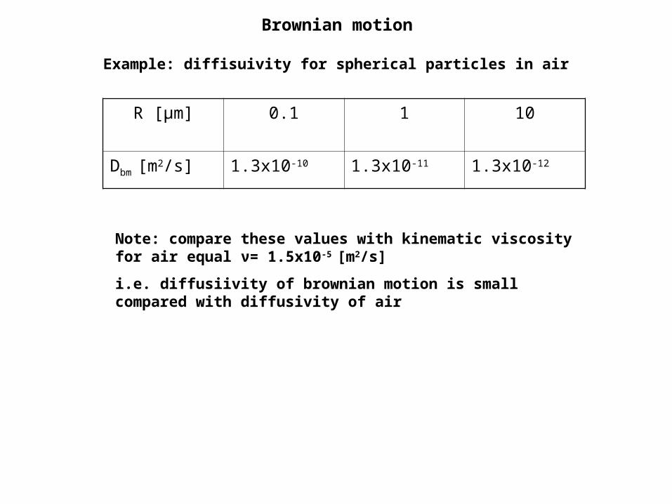
Example: diffisuivity for spherical particles in air
R [μm] 0.1 1 10
Dbm [m2/s] 1.3x10⁻¹⁰ 1.3x10⁻¹¹ 1.3x10⁻¹²
Note: compare these values with kinematic viscosity for air equal ν= 1.5x10⁻⁵ [m2/s]
i.e. diffusiivity of brownian motion is small compared with diffusivity of air
Dispersion by turbulent motion
D
dt
dDt 22
dt
d
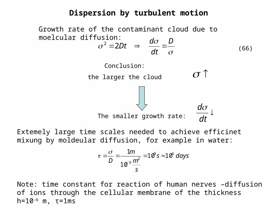
Growth rate of the contaminant cloud due to moelcular diffusion:
(66)
Conclusion:
the larger the cloud
The smaller growth rate:
Extemely large time scales needed to achieve efficinet mixung by moldeular diffusion, for example in water:
dayss
sm
m
D49
29
101010
1
Note: time constant for reaction of human nerves –diffusion of ions through the cellular membrane of the thickness h=10-6 m, τ=1ms
Dispersion by turbulent motion
How to intensify diffusion ?
A possible way to speed up diffusion
Break up the cloud into smaller fragments
If the size of the cloud is σ2, then the diffusion time scale is:
2
0
2
2
0
n
1 :is scale timediffuison theofreduction theand
is scale time then thepartssmalleer n intosplit is cloud theif ,
t
t
Dn
tD
t
n
n
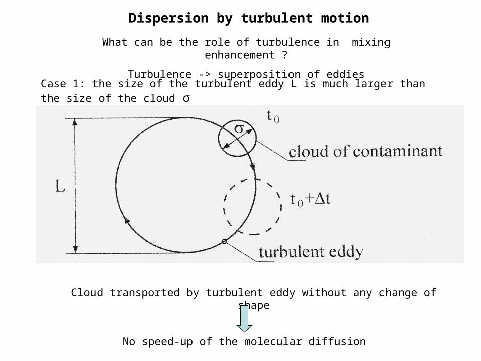
Dispersion by turbulent motion
What can be the role of turbulence in mixing enhancement ?
Turbulence -> superposition of eddies
Case 1: the size of the turbulent eddy L is much larger than the size of the cloud σ
Cloud transported by turbulent eddy without any change of shape
No speed-up of the molecular diffusion
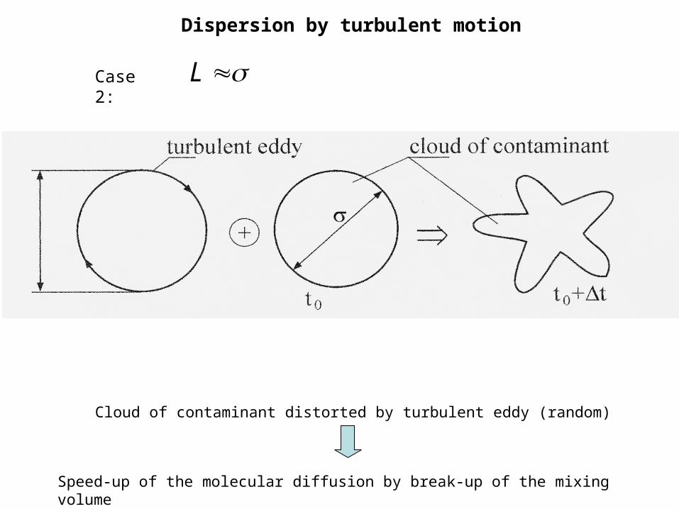
Dispersion by turbulent motion
Case 2: L
Cloud of contaminant distorted by turbulent eddy (random)
Speed-up of the molecular diffusion by break-up of the mixing volume
Dispersion by turbulent motion
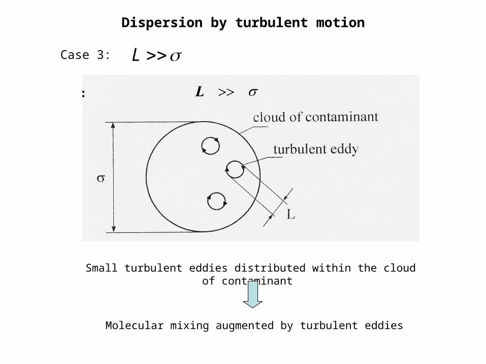
Case 3: L
Small turbulent eddies distributed within the cloud of contaminant
Molecular mixing augmented by turbulent eddies
Dispersion by turbulent motion
Possible mechanisms of turbulence interaction with molecular diffusion
Vortex stretching
Full range of eddies (from largest to smallest) appears in turbulent flow
Even if initially only largest eddies exist (case 1) after a while eddies of sizes corresponding to cases 2 and 3 will be developed
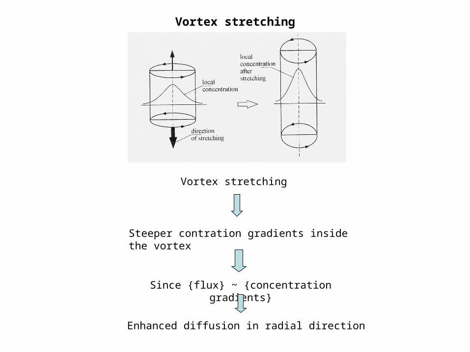
Vortex stretching
Vortex stretching
Steeper contration gradients inside the vortex
Since {flux} ~ {concentration gradients}
Enhanced diffusion in radial direction
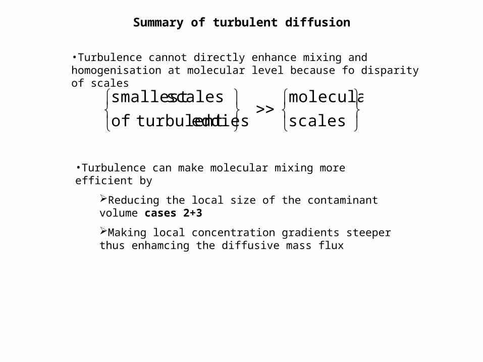
Summary of turbulent diffusion
•Turbulence cannot directly enhance mixing and homogenisation at molecular level because fo disparity of scales
scales
molecular
eddies turbulentof
scalessmallest
•Turbulence can make molecular mixing more efficient by
Reducing the local size of the contaminant volume cases 2+3
Making local concentration gradients steeper thus enhamcing the diffusive mass flux