Digital Communication with Rydberg Atoms & Amplitude-ModulatedMicrowave Fields

David H. Meyer,1, 2, a) Kevin C. Cox,2 Fredrik K. Fatemi,2 and Paul D. Kunz2, b)1)Department of Physics, University of Maryland, College Park, MD 20742,USA2)U.S. Army Research Laboratory, Sensors & Electron Devices Directorate, Adelphi, MD 20783,USA

Rydberg atoms, with one highly-excited, nearly-ionized electron, have extreme sensitivity to electric fields,including microwave fields ranging from 100 MHz to over 1 THz. Here we show that room-temperature Ryd-berg atoms can be used as sensitive, high bandwidth, microwave communication antennas. We demonstratenear photon-shot-noise limited readout of data encoded in amplitude-modulated 17 GHz microwaves, usingan electromagnetically-induced-transparency (EIT) probing scheme. We measure a photon-shot-noise limitedchannel capacity of up to 8.2 Mbit s−1 and implement an 8-state phase-shift-keying digital communicationprotocol. The bandwidth of the EIT probing scheme is found to be limited by the available coupling laserpower and the natural linewidth of the rubidium D2 transition. We discuss how atomic communicationsreceivers offer several opportunities to surpass the capabilities of classical antennas.

Rydberg atoms, created by nearly ionizing one elec-tron of a neutral atom, can be used to create exquisitelysensitive electric field sensors. This is due to the Ryd-berg atom’s dipole moment, d, which scales quadraticallywith the large, principal quantum number n, d ∼ eabn

2,where ab is the Bohr radius and e is the charge of theelectron.1 By probing many atoms at the standard quan-tum limit,2 Rydberg sensors have the potential to reachmany orders of magnitude higher sensitivity than tradi-tional electrometers,3 and have many other promising ca-pabilities including high dynamic range,4,5 SI traceabilityand self-calibration,6–8 and operation frequency spanningfrom MHz9 to THz10. However, little research has ex-plored the application of quantum sensors (like Rydbergatoms) for precise, high-bandwidth classical communica-tion using electro-magnetic fields.11

Rydberg atoms offer several exciting possibilities toexceed what is possible with classical dipole antennasfor classical digital communication. First, multiplex-ing communication using many transitions from 0.1 to1000 GHz may lead to parallel, fast communication inmultiple, widely disparate bands. Second, optically-interrogated Rydberg atoms avoid internal thermal noisethat can limit classical antennas since the internal statesof atoms can be optically pumped to effectively zero-temperature;12 the readout noise is instead limited by thequantum projection noise of either the probing light (asseen in this work) or, in the ideal case, the atoms. Evenwhen limited by the probing light, Rydberg atoms havealready been shown to have record sensitivity down to0.3 mV m−1 Hz−

1/2.13 Finally, Rydberg atomic receiverscould also, in principle, be used for sub-wavelengthimaging10,14,15 and vector detection16. Recent work hasalso shown cold Rydberg atoms can mediate direct, co-herent electro-optical conversion of MW photons into the

a)Electronic mail: dihm@terpmail.umd.edub)Electronic mail: paul.d.kunz.civ@mail.mil

+- +

-+-

+-

+-

+-

(a)

(b)

(c)

(d)

Figure 1. (a) Probe (red) and coupling (blue) light counter-propagate in a vapor cell of rubidium atoms, forming a ladder-EIT system (shown in (b)) that excites ground-state atomsto a Rydberg state. Microwaves (green) from a horn antennacouple the |50D5/2〉 and |51P3/2〉 state, and split the EITpeak. A switch modulates the microwaves, and thereby theEIT splitting, and this is detected as amplitude modulationof the probe laser intensity. (c) Probe intensity modulationcan be measured directly with a fast photodetector (d) ormeasured using an optical heterodyne, where a local oscillator(LO) beam is mixed with the transmitted probe.

optical regime via six-wave mixing.17,18 Given these po-tential strengths we introduce Rydberg atoms as a newpotential platform for digital communication worthy ofin-depth study.

In this work, we show that room-temperature Ry-dberg atoms can be used to implement a microwave-frequency (MW) receiver “antenna”19 for classical, digi-tal communication. We demonstrate phase-sensitive con-version of amplitude-modulated MW signals into opticalsignals and perform a demonstration of 8-state phase-shift-keying (PSK), the canonical digital communication

arX

iv:1

803.

0354

5v2

[ph

ysic

s.at

om-p

h] 2

9 O

ct 2

018

2

0

5 0

1 0 0

( a )V trans

/V 0 (%)

M W O f f M W O n

- 1 0 0 1 0

- 5 0

0

5 0

1 0 0

( b )

V I/V0 (%

)

P r o b e D e t u n i n g , δp ( M H z )

I

Qj m

2 5 7 5 1 2 5 1 7 50 2 2 5

- 1 8 0

- 9 0

0

9 0

1 8 0

Micro

wave

Phas

e, ϕ µ (d

eg)

T i m e ( µs )( c ) 50- 5

5

0

- 5

V Q

V I

( d )

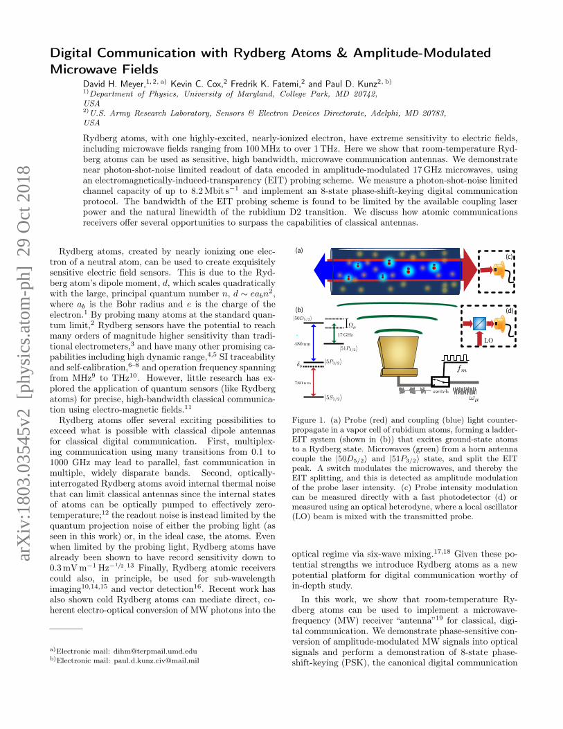
Figure 2. (a) We observe Rydberg EIT (blue) and Autler-Townes split Rydberg EIT (green) by measuring probe transmissionVtrans. (b) Example demodulated transmission signals VI with color corresponding to amplitude modulation phases φµ = 0,45, 90, 135 and 180 degrees, matching the amplitude modulation phase states shown in the inset. (c) PSK sent and receivedphase (black and red, respectively) with Ωµ = 2π× 11.4 MHz at a 40 kHz symbol frequency and an amplitude modulation rateof 1.98 MHz. The vertical dashed lines delineate the individual symbol periods. (d) Phase constellation of the received phasein (c) (red line). The axes VI and VQ are in volts measured at the lock-in amplifier. The dashed lines delineate the eight phasestates. Marker colors ranging from black to green denote the passage of one 25 µs symbol period.

protocol. We also measure the bandwidth limit of ourelectromagnetically-induced-transparency (EIT) probingscheme and observe a near photon-shot-noise limitedchannel capacity of up to 8.2 Mbit s−1 for 395 mV m−1

microwaves. Finally, we calculate the expected atom-shot-noise limited performance of a Rydberg receiver andfind it to be an order of magnitude better than thepresent measurement.

A schematic of our experimental apparatus is shownin Fig. 1(a), and the core elements are similar to thoseof other EIT-based Rydberg electrometry work4,6 (seeSupplementary Material for additional details). We usea MW horn to address a 17.0415 GHz transition be-tween the |50D5/2〉 and |51P3/2〉 states. The resonantmicrowave field establishes an Autler-Townes splitting,proportional to the MW Rabi frequency Ωµ, which isprobed using EIT, shown in Fig. 1(b). The 480 nmcoupling beam counter-propagates with respect to the780 nm probe to largely cancel Doppler-broadening of theroom-temperature atoms. To observe EIT we either di-rectly measure the transmitted probe power (Fig. 1(c))or perform heterodyne detection by interfering the probewith a 78.5 MHz-detuned local oscillator (LO).

In Figure 2(a) we present an example measurement ofprobe transmission, Vtrans, normalized to the amplitudeof the EIT peak V0, observing EIT with the microwaveson (green trace) and off (blue trace). To send digitalinformation we amplitude modulate the MW field. Themodulation phase ϕµ encodes 8 states, corresponding toall permutations of 3 bits ranging from 000 to 111. Thepossible states are shown in the I-Q plane in the inset

of 2(b). The amplitude modulation is imposed, throughEIT, onto the probe laser transmission, and the resultingoscillating probe transmission is then demodulated intoan In-Phase voltage VI and a Quadrature-Phase voltageVQ using a lock-in amplifier. Five distinct examples of thedemodulated signal VI are plotted versus probe detuningin Fig. 2(b). These VI signals are proportional to thesubtraction of two EIT signals Vtrans, with microwaveson and off, such as those shown in Fig 2(a), which leadsto features dependent on the MW Rabi frequency Ωµ asdescribed in the Supplementary Materials.

We demonstrate a PSK protocol by rapidly changingthe phase ϕµ of the amplitude modulation while mea-suring the lock-in signals at zero detuning. ϕµ is recon-structed from ϕµ = arctan(VQ/VI). Figure 2(c) showsexample sent and received amplitude-modulation phases(black and red traces respectively) where each symbolrepresenting three bits of data is transmitted for 25 µs.Figure 2(d) shows the same recovered signal in the cor-responding phase space shown in the inset of Fig. 2(b).Effective signal recovery is done when the demodulationphase is optimized (i.e. rotation of the phase space) andthe clock is properly recovered (i.e. sampling the correctset of data points spaced by the symbol send period).The data transmission rate in this experimental configu-ration is ultimately limited to ∼1 Mbit s−1 by the speedof the lock-in amplifier.20 In order to show the potentialutility of the Rydberg receiver we next characterize themore fundamental limits.

One of the most important figures of merit for any re-ceiver is the maximum channel capacity C for a single

3

- 1 . 0 - 0 . 5 0 . 0 0 . 5 1 . 00

1 02 0

( a )

Rel. T

rans.

(%)

T i m e ( µs )

0 . 1 1 1 0 1 0 0

1 0 5

1 0 6

1 0 7

1 0 8( d )

Chan

nel C

apac

ity (bi

t/s)

S y m b o l F r e q u e n c y , f s y m ( M H z )2 4 61

2

3

4

( b )Fall T

ime,

τ f (1/Γ)

A T P u m p i n g R a t e , Ω A T ( Γ )

1 2 3 4 52

4

6

( c )

Rise T

ime,

τ r (1/Γ)

E I T P u m p i n g R a t e , Ω E I T ( γ)

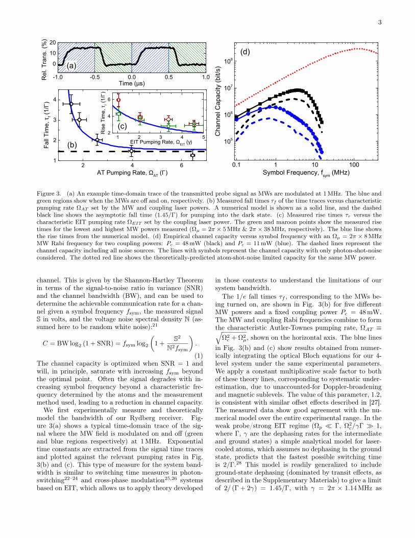
Figure 3. (a) An example time-domain trace of the transmitted probe signal as MWs are modulated at 1 MHz. The blue andgreen regions show when the MWs are off and on, respectively. (b) Measured fall times τf of the time traces versus characteristicpumping rate ΩAT set by the MW and coupling laser powers. A numerical model is shown as a solid line, and the dashedblack line shows the asymptotic fall time (1.45/Γ) for pumping into the dark state. (c) Measured rise times τr versus thecharacteristic EIT pumping rate ΩEIT set by the coupling laser power. The green and maroon points show the measured risetimes for the lowest and highest MW powers measured (Ωµ = 2π × 5 MHz & 2π × 38 MHz, respectively). The blue line showsthe rise times from the numerical model. (d) Empirical channel capacity versus symbol frequency with an Ωµ = 2π × 8 MHzMW Rabi frequency for two coupling powers: Pc = 48 mW (black) and Pc = 11 mW (blue). The dashed lines represent thechannel capacity including all noise sources. The lines with symbols represent the channel capacity with only photon-shot-noiseconsidered. The dotted red line shows the theoretically-predicted atom-shot-noise limited capacity for the same MW power.

channel. This is given by the Shannon-Hartley Theoremin terms of the signal-to-noise ratio in variance (SNR)and the channel bandwidth (BW), and can be used todetermine the achievable communication rate for a chan-nel given a symbol frequency fsym, the measured signalS in volts, and the voltage noise spectral density N (as-sumed here to be random white noise):21

C = BW log2 (1 + SNR) = fsym log2

(1 +

S2

N2fsym

).

(1)The channel capacity is optimized when SNR = 1 andwill, in principle, saturate with increasing fsym beyondthe optimal point. Often the signal degrades with in-creasing symbol frequency beyond a characteristic fre-quency determined by the atoms and the measurementmethod used, leading to a reduction in channel capacity.

We first experimentally measure and theoreticallymodel the bandwidth of our Rydberg receiver. Fig-ure 3(a) shows a typical time-domain trace of the sig-nal where the MW field is modulated on and off (greenand blue regions respectively) at 1 MHz. Exponentialtime constants are extracted from the signal time tracesand plotted against the relevant pumping rates in Fig.3(b) and (c). This type of measure for the system band-width is similar to switching time measures in photon-switching22–24 and cross-phase modulation25,26 systemsbased on EIT, which allows us to apply theory developed

in those contexts to understand the limitations of oursystem bandwidth.

The 1/e fall times τf , corresponding to the MWs be-ing turned on, are shown in Fig. 3(b) for five differentMW powers and a fixed coupling power Pc = 48 mW.The MW and coupling Rabi frequencies combine to formthe characteristic Autler-Townes pumping rate, ΩAT ≡√

Ω2c + Ω2

µ, shown on the horizontal axis. The blue linesin Fig. 3(b) and (c) show results obtained from numer-ically integrating the optical Bloch equations for our 4-level system under the same experimental parameters.We apply a constant multiplicative scale factor to bothof these theory lines, corresponding to systematic under-estimation, due to unaccounted-for Doppler-broadeningand magnetic sublevels. The value of this parameter, 1.2,is consistent with similar offset effects described in [27].The measured data show good agreement with the nu-merical model over the entire experimental range. In theweak probe/strong EIT regime (Ωp Γ, Ω2

c/γΓ 1,where Γ, γ are the dephasing rates for the intermediateand ground states) a simple analytical model for laser-cooled atoms, which assumes no dephasing in the groundstate, predicts that the fastest possible switching timeis 2/Γ.28 This model is readily generalized to includeground-state dephasing (dominated by transit effects, asdescribed in the Supplementary Materials) to give a limitof 2/ (Γ + 2γ) = 1.45/Γ, with γ = 2π × 1.14 MHz as

4

the estimated ground-state dephasing rate. The black-dashed line of Fig. 3(b) shows this limit. This analyticalprediction is also confirmed by our data.

Figure 3(c) shows the 1/e rise times corresponding tothe MWs being turned off, τr. This situation representsthe well-studied EIT pumping rate, ΩEIT ≡ Ω2

c/2Γ, for aladder EIT system and translates to the time needed toestablish the EIT dark state (i.e. resulting in greaterprobe transmission).29 We show fitted rise times forthe lowest and highest MW powers (green and maroonpoints, respectively) versus ΩEIT in units of the ground-state dephasing rate γ. In these units, ΩEIT 1 is con-sidered to be in the strong EIT regime. As expected, τrscales inversely with ΩEIT. We also see reasonable quan-titative agreement with the numerical model. In Fig. 3parts (b) and (c), for our current parameters, the bestachievable rise time τr is slower than the best fall timeτf , showing we are limited by the coupling power. How-ever, we note that for a sufficiently strong coupling laser,the fall-time limit would be the bandwidth limit for ourEIT probing scheme.

Another consideration that may affect the SNR andbandwidth is dipole-dipole interactions between ground-Rydberg states and between Rydberg-Rydberg states. Inthis work the low atom density of our vapor cell limits theeffects of interactions relative to the Doppler and transitbroadening. However, increasing the atom density to im-prove SNR or going to higher principal quantum numbersto use lower MW frequencies may lead to complicationsand increased dephasing from collisional broadening orRydberg blockade due to dipole-dipole interactions.30,31

To measure the photon-shot-noise-limited channel ca-pacity we change the measurement scheme to the het-erodyne configuration (see Fig. 1(d)). In heterodyne,gain from the LO amplifies the signal and increases thephoton-shot-noise. For sufficiently high LO powers, thephoton-shot-noise becomes the dominant noise source,allowing one to disregard other technical noise sources.We record the transmission signal amplitude S = Vtransand output voltage noise spectrum N using a spectrumanalyzer. Measuring these quantities versus the symbolfrequency (assuming one symbol per modulation period)allows us to calculate the maximum attainable channelcapacity via Eq. 1. Figure 3(d) shows the empirical chan-nel capacities for our highest (black) and lowest (blue)coupling powers. The dashed lines show the channel ca-pacity including all measured noise sources (i.e. detec-tor and laser frequency noise) while the lines with datapoints show the channel capacity with only photon-shotnoise. There are three primary regions of interest. Forlow symbol frequency the channel capacity is limited bythe modulation rate, and shows a linear rise in capacity.The channel capacity then peaks when SNR is reduced to1 by the increasing photon-shot noise and decrease in sig-nal, due to the limiting bandwidths τr and τf describedabove. For higher symbol rates the bandwidth-limitedsignal reduction dominates and the channel capacity de-creases rapidly.

The maximum empirical channel capacity for the Ωµ =2π×8 MHz MW field (395 mV m−1) shown is 8.2 Mbit s−1

at a 4 MHz symbol rate. As already described, this ca-pacity is significantly limited by the EIT probing schemeand the associated photon shot-noise. Even so, the sensi-tivity of the photon-shot-noise limited Rydberg receiverdetecting a ∼ 13 mV m−1 MW field allows for a channelcapacity of 10 kbit s−1 which is sufficient for some appli-cations such as audio transmission.

However, the photon-shot-noise that is limiting ourcurrent measurement is not a fundamental limit. Wave-function collapse limits the SNR when using Rydbergatoms, or any other sensor made of 2-level quantumsystems, to the Standard Quantum Limit for measure-ment of a quantum phase φ. For classical communica-tion the maximum possible accumulated phase for onetransmitted symbol is φ = Ωµ · tm, assuming a coherencetime longer than the symbol period tm = 1/fm. Thestandard quantum limited phase uncertainty is ∆φ =1/√N , where N is the number of qubits (atom num-

ber in our case).2 This leads to a quantum-limited SNR,SNRq = NΩ2

µ/f2m, and theoretical channel capacity,

Cq = fm log2

(1 +NΩ2

µ/f2m

). This capacity is optimized

when fm ≈√NΩµ/2, leading to an optimum quantum-

limited capacity of Coptq ≈√NΩµ log2(5)/2. The red

line of Figure 3(d) shows this predicted channel capacityfor the same MW field. The maximum channel capacityfor 1000 atoms is predicted to be ∼ 292 Mbit s−1, a morethan 30-fold increase over the current maximum attainedwith photon-shot-noise. Finding a way to achieve thestandard quantum limit with room-temperature Rydbergsensors is a significant avenue for further research. Due toEIT’s inherent photon-shot-noise and bandwidth limitsthat we have characterized here, other probing schemesmay be advantageous. Recently realized alternatives thatdo not rely on optical probing include state-selective ion-ization of the Rydberg state followed by detection witha multi-channel plate.32,33 Electro-optic conversion fromMW to optical fields, while different than what we havedemonstrated (EIT probing converts only the modulationfromMW to optical fields), is another alternative.18 How-ever, high efficiency operation requires mode-matchingthe MW field to the mode volume of the mixing lightfields,17 which can be difficult for free space communica-tions.

Notably, the quantum-limited channel capacity doesnot a function of the carrier frequency. This is signifi-cantly different from the standard data transmission limitfor electrically small antennas, often referred to as theChu limit, which states that the characteristic qualityfactor (inverse fractional bandwidth) of an electrically-small, efficient antenna is Q ≈ 1/(k3a3) where a is thesize of the antenna and k is the wave-vector of the MWfield.34,35 In contrast, Rydberg atomic sensors can beused with a characteristic size of a few micrometers,36while generally maintaining their bandwidth. As a quan-titative comparison, consider the 802.11ac Wi-Fi stan-dard for a 5 GHz carrier. This standard has a maxi-

5

mum single channel data rate of 867 Mbit s−1 at a BW of160 MHz.37 However, if one were to use an efficient, elec-trically small antenna 500 µm in size (a cell size readilyachievable with Rydberg atoms36) the BW would be re-duced to less than 90 kHz, significantly reducing the datarate. This comparison is somewhat simplistic; atoms andclassical antennas measure electric fields in fundamen-tally different ways, and an in-depth comparison shouldbe the subject of future work. However, it highlights apotential regime where atomic sensors may significantlyoutperform a fundamental limit of classical antennas forcommunication. Rydberg quantum sensors may offeran alternative approach to achieve simultaneously small,high speed, and exquisitely sensitive receivers. As pre-viously mentioned, they also have many additional at-tractive properties: because there are so many avail-able Rydberg states, changing the carrier frequency onlyamounts to changing the laser frequency, requiring nomoving parts; vector detection and sub-wavelength imag-ing are also possible. Further study, beyond the scope ofthis initial work, will be required to discover the preciseapplications where Rydberg quantum sensors can outper-form existing antennas. Nonetheless, this system holdssignificant promise to become one of a small number ofuseful technologies operating in the quantum regime.

SUPPLEMENTARY MATERIAL

See supplementary material for a detailed descriptionof the experimental apparatus, the demodulated signaldependence on MW Rabi frequency, and the derivationof the τf limit for a transit-broadened medium.

ACKNOWLEDGMENTS

This work was partially supported by the Oak RidgeAssociated Universities and the Quantum Science & En-gineering Program of the Office of the Secretary of De-fense.

REFERENCES

1T. Gallagher, Rydberg Atoms, 1st ed., Cambridge Monographson Atomic, Molecular and Chemical Physics No. 3 (CambridgeUniversity Press, Cambridge, 2005).

2D. J. Wineland, J. J. Bollinger, W. M. Itano, and D. J. Heinzen,Physical Review A 50, 67 (1994).

3H. Fan, S. Kumar, J. Sedlacek, H. Kübler, S. Karimkashi, andJ. P. Shaffer, Journal of Physics B: Atomic, Molecular and Op-tical Physics 48, 202001 (2015).

4J. A. Sedlacek, A. Schwettmann, H. Kübler, R. Löw, T. Pfau,and J. P. Shaffer, Nature Physics 8, 819 (2012).

5D. A. Anderson, S. A. Miller, G. Raithel, J. A. Gordon, M. L.Butler, and C. L. Holloway, Physical Review Applied 5, 034003(2016).

6C. Holloway, J. Gordon, S. Jefferts, A. Schwarzkopf, D. Ander-son, S. Miller, N. Thaicharoen, and G. Raithel, IEEE Transac-tions on Antennas and Propagation 62, 6169 (2014).

7M. T. Simons, J. A. Gordon, and C. L. Holloway, Journal ofApplied Physics 120, 123103 (2016).

8C. L. Holloway, M. T. Simons, J. A. Gordon, A. Dienstfrey,D. A. Anderson, and G. Raithel, Journal of Applied Physics121, 233106 (2017).

9S. A. Miller, D. A. Anderson, and G. Raithel, New Journal ofPhysics 18, 053017 (2016).

10C. G. Wade, N. Šibalić, N. R. de Melo, J. M. Kondo, C. S. Adams,and K. J. Weatherill, Nature Photonics 11, 40 (2017).

11V. Gerginov, F. C. S. da Silva, and D. Howe, Review of ScientificInstruments 88, 125005 (2017).

12R. A. Bernheim, Optical Pumping: An Introduction, Frontiers inChemistry (W. A. Benjamin, Inc., New York, 1965).

13S. Kumar, H. Fan, H. Kübler, A. J. Jahangiri, and J. P. Shaffer,Optics Express 25, 8625 (2017).

14C. L. Holloway, J. A. Gordon, A. Schwarzkopf, D. A. Anderson,S. A. Miller, N. Thaicharoen, and G. Raithel, Applied PhysicsLetters 104, 244102 (2014).

15H. Q. Fan, S. Kumar, R. Daschner, H. Kübler, and J. P. Shaffer,Optics Letters 39, 3030 (2014).

16J. A. Sedlacek, A. Schwettmann, H. Kübler, and J. P. Shaffer,Physical Review Letters 111, 063001 (2013).

17M. Kiffner, A. Feizpour, K. T. Kaczmarek, D. Jaksch, andJ. Nunn, New Journal of Physics 18, 093030 (2016).

18J. Han, T. Vogt, C. Gross, D. Jaksch, M. Kiffner, and W. Li,Physical Review Letters 120, 093201 (2018).

19Our driven atomic sensor may not satisfy the definition of anantenna used in classical antenna theory since it breaks severalcommon assumptions. Most importantly our atomic receiver isnot passive, and actually performs a non-destructive measure-ment of the field.

20This is due to the lock-in amplifier’s minimum output time con-stant of 1µs which limits the symbol rate.

21L. S. Hanzo and W. Webb, Single- and Multi-Carrier QuadratureAmplitude Modulation (John Wiley & Sons, Ltd., 2000).

22S. E. Harris and Y. Yamamoto, Physical Review Letters 81, 3611(1998).

23M. Yan, E. G. Rickey, and Y. Zhu, Physical Review A 64, 041801(2001).

24D. A. Braje, V. Balić, G. Y. Yin, and S. E. Harris, PhysicalReview A 68, 041801 (2003).

25H. Schmidt and A. Imamoglu, Optics Letters 21, 1936 (1996).26M. Fleischhauer, A. Imamoglu, and J. P. Marangos, Reviews ofModern Physics 77, 633 (2005).

27G. Dmochowski, A. Feizpour, M. Hallaji, C. Zhuang, A. Hayat,and A. M. Steinberg, Physical Review Letters 116, 173002(2016).

28Y.-F. Chen, G.-C. Pan, and I. A. Yu, Physical Review A 69,063801 (2004).

29A. Feizpour, G. Dmochowski, and A. M. Steinberg, PhysicalReview A 93, 013834 (2016).

30A. Urvoy, F. Ripka, I. Lesanovsky, D. Booth, J. P. Shaffer,T. Pfau, and R. Löw, Physical Review Letters 114, 203002(2015).

31D. Kara, A. Bhowmick, and A. K. Mohapatra, Scientific Reports8, 5256 (2018).

32A. Facon, E.-K. Dietsche, D. Grosso, S. Haroche, J.-M. Raimond,M. Brune, and S. Gleyzes, Nature 535, 262 (2016).

33J. Koepsell, T. Thiele, J. Deiglmayr, A. Wallraff, and F. Merkt,Physical Review A 95, 053860 (2017).

34H. A. Wheeler, Proceedings of the IRE 35, 1479 (1947).35L. J. Chu, Journal of Applied Physics 19, 1163 (1948).36H. Kübler, J. P. Shaffer, T. Baluktsian, R. Löw, and T. Pfau,Nature Photonics 4, 112 (2010).

37IEEE Std 802.11ac(TM)-2013 (Amendment to IEEE Std 802.11-2012, as amended by IEEE Std 802.11ae-2012, IEEE Std802.11aa-2012, and IEEE Std 802.11ad-2012) , 1 (2013).

38P. T. Starkey, C. J. Billington, S. P. Johnstone, M. Jasperse,K. Helmerson, L. D. Turner, and R. P. Anderson, Review ofScientific Instruments 84, 085111 (2013).

6

39A. Sargsyan, M. G. Bason, D. Sarkisyan, A. K. Mohapatra, andC. S. Adams, Optics and Spectroscopy 109, 529 (2010).

40M. Mack, F. Karlewski, H. Hattermann, S. Höckh, F. Jessen,D. Cano, and J. Fortágh, Physical Review A 83, 052515 (2011).

41J. Sagle, R. K. Namiotka, and J. Huennekens, Journal of PhysicsB: Atomic, Molecular and Optical Physics 29, 2629 (1996).

7

Supplementary Materials for Digital Communication with Rydberg Atoms &Amplitude-Modulated Microwave Fields

EXPERIMENTAL DETAILS

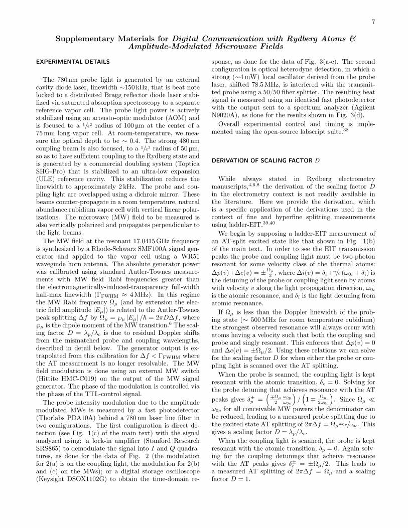
The 780 nm probe light is generated by an externalcavity diode laser, linewidth ∼150 kHz, that is beat-notelocked to a distributed Bragg reflector diode laser stabi-lized via saturated absorption spectroscopy to a separatereference vapor cell. The probe light power is activelystabilized using an acousto-optic modulator (AOM) andis focused to a 1/e2 radius of 100 µm at the center of a75 mm long vapor cell. At room-temperature, we mea-sure the optical depth to be ∼ 0.4. The strong 480 nmcoupling beam is also focused, to a 1/e2 radius of 50 µm,so as to have sufficient coupling to the Rydberg state andis generated by a commercial doubling system (TopticaSHG-Pro) that is stabilized to an ultra-low expansion(ULE) reference cavity. This stabilization reduces thelinewidth to approximately 2 kHz. The probe and cou-pling light are overlapped using a dichroic mirror. Thesebeams counter-propagate in a room temperature, naturalabundance rubidium vapor cell with vertical linear polar-izations. The microwave (MW) field to be measured isalso vertically polarized and propagates perpendicular tothe light beams.

The MW field at the resonant 17.0415 GHz frequencyis synthesized by a Rhode-Schwarz SMF100A signal gen-erator and applied to the vapor cell using a WR51waveguide horn antenna. The absolute generator powerwas calibrated using standard Autler-Townes measure-ments with MW field Rabi frequencies greater thanthe electromagnetically-induced-transparency full-widthhalf-max linewidth (ΓFWHM ≈ 4 MHz). In this regimethe MW Rabi frequency Ωµ (and by extension the elec-tric field amplitude |Eµ|) is related to the Autler-Townespeak splitting ∆f by Ωµ = ℘µ |Eµ| /~ = 2πD∆f , where℘µ is the dipole moment of the MW transition.6 The scal-ing factor D = λp/λc is due to residual Doppler shiftsfrom the mismatched probe and coupling wavelengths,described in detail below. The generator output is ex-trapolated from this calibration for ∆f < ΓFWHM wherethe AT measurement is no longer resolvable. The MWfield modulation is done using an external MW switch(Hittite HMC-C019) on the output of the MW signalgenerator. The phase of the modulation is controlled viathe phase of the TTL-control signal.

The probe intensity modulation due to the amplitudemodulated MWs is measured by a fast photodetector(Thorlabs PDA10A) behind a 780 nm laser line filter intwo configurations. The first configuration is direct de-tection (see Fig. 1(c) of the main text) with the signalanalyzed using: a lock-in amplifier (Stanford ResearchSRS865) to demodulate the signal into I and Q quadra-tures, as done for the data of Fig. 2 (the modulationfor 2(a) is on the coupling light, the modulation for 2(b)and (c) on the MWs); or a digital storage oscilloscope(Keysight DSOX1102G) to obtain the time-domain re-

sponse, as done for the data of Fig. 3(a-c). The secondconfiguration is optical heterodyne detection, in which astrong (∼4 mW) local oscillator derived from the probelaser, shifted 78.5 MHz, is interfered with the transmit-ted probe using a 50/50 fiber splitter. The resulting beatsignal is measured using an identical fast photodetectorwith the output sent to a spectrum analyzer (AgilentN9020A), as done for the results shown in Fig. 3(d).

Overall experimental control and timing is imple-mented using the open-source labscript suite.38

DERIVATION OF SCALING FACTOR D

While always stated in Rydberg electrometrymanuscripts,4,6,8 the derivation of the scaling factor Din the electrometry context is not readily available inthe literature. Here we provide the derivation, whichis a specific application of the derivations used in thecontext of fine and hyperfine splitting measurementsusing ladder-EIT.39,40

We begin by supposing a ladder-EIT measurement ofan AT-split excited state like that shown in Fig. 1(b)of the main text. In order to see the EIT transmissionpeaks the probe and coupling light must be two-photonresonant for some velocity class of the thermal atoms:∆p(v)+∆c(v) = ±Ωµ

2 , where ∆i(v) = δi+v/c (ω0i + δi) isthe detuning of the probe or coupling light seen by atomswith velocity v along the light propagation direction, ω0i

is the atomic resonance, and δi is the light detuning fromatomic resonance.

If Ωµ is less than the Doppler linewidth of the prob-ing state (∼ 500 MHz for room temperature rubidium)the strongest observed resonance will always occur withatoms having a velocity such that both the coupling andprobe and singly resonant. This enforces that ∆p(v) = 0and ∆c(v) = ±Ωµ/2. Using these relations we can solvefor the scaling factor D for when either the probe or cou-pling light is scanned over the AT splitting.

When the probe is scanned, the coupling light is keptresonant with the atomic transition, δc = 0. Solving forthe probe detuning that achieves resonance with the ATpeaks gives δ±p =

(∓Ωµ

2ω0p

ω0c

)/(

1∓ Ωµ2ω0c

). Since Ωµ

ω0c for all conceivable MW powers the denominator canbe reduced, leading to a measured probe splitting due tothe excited state AT splitting of 2π∆f = Ωµω0p/ω0c. Thisgives a scaling factor D = λp/λc.

When the coupling light is scanned, the probe is keptresonant with the atomic transition, δp = 0. Again solv-ing for the coupling detunings that acheive resonancewith the AT peaks gives δ±c = ±Ωµ/2. This leads toa measured AT splitting of 2π∆f = Ωµ and a scalingfactor D = 1.

8

0 5 1 0 1 5

02468

1 01 2

0 . 1 1 1 00

1

Splitti

ng (M

Hz)

M W R a b i F r e q u e n c y , Ωµ/ 2 π ( M H z )

( a )

( b )

Signa

l Amp

litude

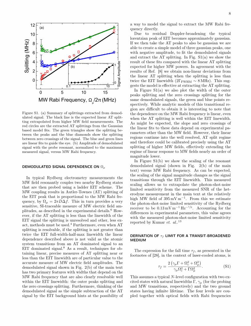
Figure S1. (a) Summary of splittings extracted from demod-ulated signal. The black line is the expected linear AT split-ting extrapolated from higher MW field measurements. Thered circles are the extracted AT splittings from the Gaussianbased model fits. The green triangles show the splitting be-tween the peaks and the blue diamonds show the splittingbetween zero crossings of the signal. The blue and green linesare linear fits to guide the eye. (b) Amplitude of demodulatedsignal with the probe resonant, normalized to the maximummeasured signal, versus MW Rabi frequency.

DEMODULATED SIGNAL DEPENDENCE ON Ωµ

In typical Rydberg electrometry measurements theMW field resonantly couples two nearby Rydberg statesthat are then probed using a ladder EIT scheme. TheMW coupling results in Autler-Townes (AT) splitting ofthe EIT peak that is proportional to the MW Rabi fre-quency, by Ωµ = 2πD∆f . This in turn provides a verysensitive, SI-traceable measure of MW electric field am-plitudes, as described in the experimental details.6 How-ever, if the AT splitting is less than the linewidth of theEIT signal the splitting is unresolved and other, less ex-act, methods must be used.4 Furthermore, even when ATsplitting is resolvable, if the splitting is not greater thantwice the EIT full-width-half-max linewidth the lineardependence described above is not valid as the atomicsystem transitions from an AT dominated signal to anEIT dominated signal.8 As a result, techniques for ob-taining linear, precise measures of AT splitting near orless than the EIT linewidth are of particular value to theaccurate measure of MW electric field amplitudes. Thedemodulated signal shown in Fig. 2(b) of the main texthas two primary features with widths that depend on theMW Rabi frequency that are also clearly resolvable wellwithin the EIT linewidth: the outer peaks splitting andthe zero crossings splitting. Furthermore, thinking of thedemodulated signal as the simple subtraction of the ATsignal by the EIT background hints at the possibility of

a way to model the signal to extract the MW Rabi fre-quency directly.

Due to residual Doppler-broadening the typicallorentzian peak of EIT becomes approximately gaussian.If we then take the AT peaks to also be gaussian we areable to create a simple model of three gaussian peaks, onewith negative amplitude, to fit the demodulated signalsand extract the AT splitting. In Fig. S1(a) we show theresult of these fits compared with the linear AT splittingexpected for higher MW powers. In agreement with theresults of Ref. [8] we obtain non-linear deviations fromthe linear AT splitting when the splitting is less thantwice the EIT linewidth (2ΓFWHM ∼ 8 MHz). This sug-gests the model is effective at extracting the AT splitting.

In Figure S1(a) we also plot the width of the outerpeaks splitting and the zero crossings splitting for thesame demodulated signals, the green and blue points re-spectively. While analytic models of this transitional re-gion are difficult to obtain it is interesting to note thatthe dependence on the MW Rabi frequency is linear, evenwhen the AT splitting is well within the EIT linewidth.As might be expected, the slope and zero crossings ofthe linear fits to these data depend on experimental pa-rameters other than the MW field. However, their linearregions continue into the well resolved, AT split regimeand therefore could be calibrated precisely using the ATsplitting of higher MW fields, effectively extending theregime of linear response to MW fields nearly an order ofmagnitude lower.

In Figure S1(b) we show the scaling of the resonantdemodulated signal (shown in Fig. 2(b) of the maintext) versus MW Rabi frequency. As can be expected,the scaling of the signal magnitude changes as the signaltransitions through the EIT linewidth. This measuredscaling allows us to extrapolate the photon-shot-noiselimited sensitivity from the measured SNR of the het-erodyne measurement in the main text at the relativelyhigh MW field of 395 mV m−1. From this we estimatethe photon-shot-noise limited sensitivity of the Rydbergreceiver to be 0.13 mV m−1 Hz−

1/2. Accounting for thedifferences in experimental parameters, this value agreeswith the measured photon-shot-noise limited sensitivityreported by Kumar et. al..13

DERIVATION OF τf LIMIT FOR A TRANSIT-BROADENEDMEDIUM

The expression for the fall time τf , as presented in thefootnotes of [28], in the context of laser-cooled atoms, is

τf =2(γµΓ + Ω2

c + Ω2µ

)γµΩ2

c + ΓΩ2µ

. (S1)

This assumes a typical N -level configuration with two ex-cited states with natural linewidths Γ, γµ (for the probingand MW transitions, respectively) and the two groundstates having infinite lifetime. The four levels are cou-pled together with optical fields with Rabi frequencies

9

4 6 8

2

3

Fall T

ime,

τ f (1/Γ)

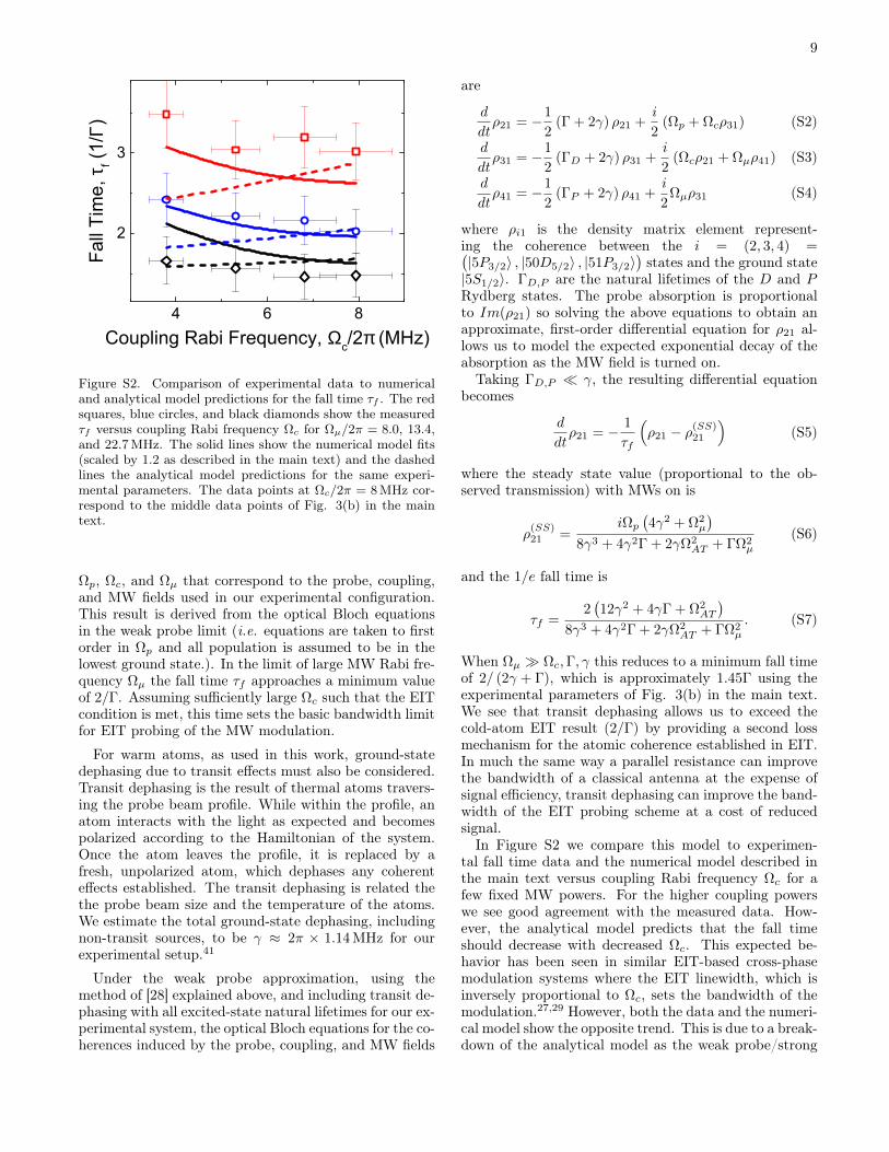
C o u p l i n g R a b i F r e q u e n c y , Ωc / 2 π ( M H z )Figure S2. Comparison of experimental data to numericaland analytical model predictions for the fall time τf . The redsquares, blue circles, and black diamonds show the measuredτf versus coupling Rabi frequency Ωc for Ωµ/2π = 8.0, 13.4,and 22.7 MHz. The solid lines show the numerical model fits(scaled by 1.2 as described in the main text) and the dashedlines the analytical model predictions for the same experi-mental parameters. The data points at Ωc/2π = 8 MHz cor-respond to the middle data points of Fig. 3(b) in the maintext.

Ωp, Ωc, and Ωµ that correspond to the probe, coupling,and MW fields used in our experimental configuration.This result is derived from the optical Bloch equationsin the weak probe limit (i.e. equations are taken to firstorder in Ωp and all population is assumed to be in thelowest ground state.). In the limit of large MW Rabi fre-quency Ωµ the fall time τf approaches a minimum valueof 2/Γ. Assuming sufficiently large Ωc such that the EITcondition is met, this time sets the basic bandwidth limitfor EIT probing of the MW modulation.

For warm atoms, as used in this work, ground-statedephasing due to transit effects must also be considered.Transit dephasing is the result of thermal atoms travers-ing the probe beam profile. While within the profile, anatom interacts with the light as expected and becomespolarized according to the Hamiltonian of the system.Once the atom leaves the profile, it is replaced by afresh, unpolarized atom, which dephases any coherenteffects established. The transit dephasing is related thethe probe beam size and the temperature of the atoms.We estimate the total ground-state dephasing, includingnon-transit sources, to be γ ≈ 2π × 1.14 MHz for ourexperimental setup.41

Under the weak probe approximation, using themethod of [28] explained above, and including transit de-phasing with all excited-state natural lifetimes for our ex-perimental system, the optical Bloch equations for the co-herences induced by the probe, coupling, and MW fields

are

d

dtρ21 = −1

2(Γ + 2γ) ρ21 +

i

2(Ωp + Ωcρ31) (S2)

d

dtρ31 = −1

2(ΓD + 2γ) ρ31 +

i

2(Ωcρ21 + Ωµρ41) (S3)

d

dtρ41 = −1

2(ΓP + 2γ) ρ41 +

i

2Ωµρ31 (S4)

where ρi1 is the density matrix element represent-ing the coherence between the i = (2, 3, 4) =(|5P3/2〉 , |50D5/2〉 , |51P3/2〉

)states and the ground state

|5S1/2〉. ΓD,P are the natural lifetimes of the D and PRydberg states. The probe absorption is proportionalto Im(ρ21) so solving the above equations to obtain anapproximate, first-order differential equation for ρ21 al-lows us to model the expected exponential decay of theabsorption as the MW field is turned on.

Taking ΓD,P γ, the resulting differential equationbecomes

d

dtρ21 = − 1

τf

(ρ21 − ρ(SS)

21

)(S5)

where the steady state value (proportional to the ob-served transmission) with MWs on is

ρ(SS)21 =

iΩp(4γ2 + Ω2

µ

)8γ3 + 4γ2Γ + 2γΩ2

AT + ΓΩ2µ

(S6)

and the 1/e fall time is

τf =2(12γ2 + 4γΓ + Ω2

AT

)8γ3 + 4γ2Γ + 2γΩ2

AT + ΓΩ2µ

. (S7)

When Ωµ Ωc,Γ, γ this reduces to a minimum fall timeof 2/ (2γ + Γ), which is approximately 1.45Γ using theexperimental parameters of Fig. 3(b) in the main text.We see that transit dephasing allows us to exceed thecold-atom EIT result (2/Γ) by providing a second lossmechanism for the atomic coherence established in EIT.In much the same way a parallel resistance can improvethe bandwidth of a classical antenna at the expense ofsignal efficiency, transit dephasing can improve the band-width of the EIT probing scheme at a cost of reducedsignal.

In Figure S2 we compare this model to experimen-tal fall time data and the numerical model described inthe main text versus coupling Rabi frequency Ωc for afew fixed MW powers. For the higher coupling powerswe see good agreement with the measured data. How-ever, the analytical model predicts that the fall timeshould decrease with decreased Ωc. This expected be-havior has been seen in similar EIT-based cross-phasemodulation systems where the EIT linewidth, which isinversely proportional to Ωc, sets the bandwidth of themodulation.27,29 However, both the data and the numeri-cal model show the opposite trend. This is due to a break-down of the analytical model as the weak probe/strong

10

EIT regime assumption becomes less valid. As mentionedin the main text, the EIT regime is when Ω2

c/Γγ 1which is only approximately true for the data presented.In this weak EIT regime greater Ωc leads to a strongerEIT signal that effectively has a larger linewidth andtherefore bandwidth.

In short, increased coupling power to fully obtain theEIT regime is necessary for greater signal bandwidth.However, increasing the coupling power well beyond theEIT regime will eventually lead to reduced signal band-width as the EIT linewidth is narrowed.