Embed Size (px)
Citation preview

Lecture
DIGITAL PROCESSING
OF
SPEECH AND IMAGE SIGNALS
RWTH Aachen, WS 2006/7
Prof. Dr.-Ing. H. Ney, Dr.rer.nat. R. SchluterLehrstuhl fur Informatik 6
RWTH Aachen
1. System Theory and Fourier Transform
2. Discrete Time Systems
3. Spectral Analysis
4. Fourier Transform and Image Processing
5. LPC Analysis
6. Wavelets
7. Coding
8. Image Segmentation and Contour-Finding
Completions: L. Welling, A. Eiden; April 1997Completions: J. Dahmen, F. Hilger, S. Koepke; Mai 2000Completions: F. Hilger, D. Keysers; Juli 2001Translation: M. Popovic, R. Schluter; April 2003Corrections: D. Stein; October 2006
Literature:
• A. V. Oppenheim, R. W. Schafer: Discrete Time Signal Processing,Prentice Hall, Englewood Cliffs, NJ, 1989.
• A. Papoulis: Signal Analysis, McGraw-Hill, New York, NY, 1977.
• A. Papoulis: The Fourier Integral and its Applications, McGraw-HillClassic Textbook Reissue Series, McGraw-Hill, New York, NY, 1987.
• W. K. Pratt: Digital Image Processing, Wiley & Sons Inc, New York,NY, 1991.
Further reading:
• T. K. Moon, W. C. Stirling: Mathematical Methods and Algorithms
for Signal Processing. Prentice Hall, Upper Saddle River, NJ, 2000.
• J. R. Deller, J. G. Proakis, J. H. L. Hansen: Discrete-Time Processingof Speech Signals, Macmillan Publishing Company, New York, NY,1993.
• W. H. Press, S. A. Teukolsky, W. T. Vetterling, B. P. Flannery: Nu-merical Recipes in C, Cambridge Univ. Press, Cambridge, 1992.
• L. Rabiner, B. H. Juang: Fundamentals of Speech Recognition, Pren-tice Hall, Englewood Cliffs, NJ, 1993.
• T. Lehmann, W. Oberschelp, E. Pelikan, R. Repges: Bildverarbeitungfur die Medizin, Springer Verlag, Berlin, 1997.
• L. Berg: Lineare Gleichungssysteme mit Bandstruktur, VEB DeutscherVerlag der Wissenschaften, Berlin, 1986.
Contents
1 System Theory and Fourier Transform 1
1.1 Introduction . . . . . . . . . . . . . . . . . . . . . . . . . . 2
1.2 Linear time-invariant Systems . . . . . . . . . . . . . . . . 11
1.3 Fourier Transform . . . . . . . . . . . . . . . . . . . . . . . 16
1.4 Properties of the Fourier Transform . . . . . . . . . . . . . 25
1.5 Parseval Theorem . . . . . . . . . . . . . . . . . . . . . . . 33
1.6 Autocorrelation Function . . . . . . . . . . . . . . . . . . . 34
1.7 Existence of the Fourier Transform . . . . . . . . . . . . . 35
1.8 δ-Function . . . . . . . . . . . . . . . . . . . . . . . . . . . 36
1.9 Motivation for Fourier Series . . . . . . . . . . . . . . . . . 41
1.10 Time Duration and Band Width . . . . . . . . . . . . . . . 45
2 Discrete Time Systems 51
2.1 Motivation and Goal . . . . . . . . . . . . . . . . . . . . . 52
2.2 Digital Simulation using Discrete Time Systems . . . . . . 53
2.3 Examples of Discrete Time Systems . . . . . . . . . . . . . 56
2.4 Sampling Theorem (Nyquist Theorem) and Reconstruction 61
2.5 Logarithmic Scale and dB . . . . . . . . . . . . . . . . . . 70
2.6 Quantization . . . . . . . . . . . . . . . . . . . . . . . . . 72
2.7 Fourier Transform and z–Transform . . . . . . . . . . . . . 74
2.8 System Representation and Examples . . . . . . . . . . . . 78
2.9 Discrete Time Signal Fourier Transform Theorem . . . . . 88
2.10 Discrete Fourier Transform: DFT . . . . . . . . . . . . . . 90
2.11 DFT as Matrix Operation . . . . . . . . . . . . . . . . . . 98
2.12 From Continuous Fourier Transform to Matrix Representa-tion of Discrete Fourier Transform . . . . . . . . . . . . . . 102
2.13 Frequency Resolution and Zero Padding . . . . . . . . . . 104
2.14 Finite Convolution . . . . . . . . . . . . . . . . . . . . . . 105
2.15 Fast Fourier Transform (FFT) . . . . . . . . . . . . . . . . 108
2.16 FFT Implementation . . . . . . . . . . . . . . . . . . . . . 118
i

2.17 Cyclic Matrices and Fourier Transform . . . . . . . . . . . 124
3 Spectral analysis 1313.1 Features for Speech Recognition . . . . . . . . . . . . . . . 1323.2 Short Time Analysis and Windowing . . . . . . . . . . . . 1353.3 Autocorrelation Function and Power Spectral Density . . . 1593.4 Spectrograms . . . . . . . . . . . . . . . . . . . . . . . . . 1653.5 Filter Bank Analysis . . . . . . . . . . . . . . . . . . . . . 1683.6 Mel-frequency scale . . . . . . . . . . . . . . . . . . . . . . 1713.7 Cepstrum . . . . . . . . . . . . . . . . . . . . . . . . . . . 1733.8 Statistical Interpretation of the Cepstrum Transformation 1833.9 Energy in acoustic Vector . . . . . . . . . . . . . . . . . . 185
4 Fourier Transform and Image Processing 1874.1 Spatial Frequencies and Fourier Transform for Images . . . 1884.2 Discrete Fourier Transform for Images . . . . . . . . . . . 1964.3 Fourier Transform in Computer Tomography . . . . . . . . 1974.4 Fourier Transform and RST Invariance . . . . . . . . . . . 199
5 LPC Analysis 2075.1 Principle of LPC Analysis . . . . . . . . . . . . . . . . . . 2085.2 LPC: Covariance Method . . . . . . . . . . . . . . . . . . . 2125.3 LPC: Autocorrelation Method . . . . . . . . . . . . . . . . 2135.4 LPC: Interpretation in Frequency Domain . . . . . . . . . 2165.5 LPC: Generative Model . . . . . . . . . . . . . . . . . . . 2215.6 LPC: Alternative Representations . . . . . . . . . . . . . . 223
6 Outlook: Wavelet Transform 2256.1 Motivation: from Fourier to Wavelet Transform . . . . . . 2266.2 Definition . . . . . . . . . . . . . . . . . . . . . . . . . . . 2276.3 Discrete Wavelet Transform . . . . . . . . . . . . . . . . . 229
7 Coding (appendix available as separate document) 233
8 Image Segmentation and Contour-Finding 237
ii

List of Figures
1.1 Oscillograms of three time functions composed as sum of 20partial oscillations. a) φn = 0, b) φn = π
2 , c) φn statistical. 3
1.2 Amplitude spectrum of a time function composed as sum of20 partial tones. . . . . . . . . . . . . . . . . . . . . . . . . 3
1.3 from left to right: original photo, low-pass and high-passfiltered version . . . . . . . . . . . . . . . . . . . . . . . . 3
1.4 Phase manipulation for portion of a speech signal (vowel ’o’)sampled at 8kHz, 25ms analysis window (200 samples), 512point FFT . . . . . . . . . . . . . . . . . . . . . . . . . . . 4
1.5 Phase manipulation for portion of a speech signal (consonant’n’) sampled at 8kHz, 25ms analysis window (200 samples),512 point FFT . . . . . . . . . . . . . . . . . . . . . . . . 5
1.6 Phase manipulation for a Heaviside–function (step–function) 6
1.7 Schematic representation of the physiological mechanism ofspeech production . . . . . . . . . . . . . . . . . . . . . . . 8
2.1 Digital photo . . . . . . . . . . . . . . . . . . . . . . . . . 58
2.2 Gradient image . . . . . . . . . . . . . . . . . . . . . . . . 58
2.3 Several real cases of Laplace Operator subtraction from orig-inal image. a) Original image b) Original image minusLaplace Operator (negative values are set to 0 and valuesabove the grey scale are set to the highest grade of grey) . 60
2.4 Ideal reconstruction of a band-limited signal (from Oppen-heim, Schafer)a) original signal b) sampled signal c) reconstructed signal 64
iii

2.5 Sampling of band-limited signal with different sampling rates:b) sampling rate higher than Nyquist rate - exact reconstruc-tion possiblec) sampling rate equal to Nyquist rate - exact reconstructionpossibled) sampling rate smaller than Nyquist rate - aliasing - exactreconstruction not possible . . . . . . . . . . . . . . . . . . 65
2.6 Amplitude spectrum of the voiceless phoneme “s” from theword “ist” . . . . . . . . . . . . . . . . . . . . . . . . . . . 71
2.7 Logarithmic amplitude spectrum of the phoneme “s” . . . 71
2.8 Amplitude spectrum of the voiced phoneme “ae” from theword “Ah” . . . . . . . . . . . . . . . . . . . . . . . . . . . 71
2.9 Logarithmic amplitude spectrum of the phoneme “ae” . . . 71
2.10 Amplitude spectrum of a speech pause . . . . . . . . . . . 71
2.11 Logarithmic amplitude spectrum of a speech pause . . . . 71
2.12 Hanning window . . . . . . . . . . . . . . . . . . . . . . . 103
2.13 Example of a linear convolution of two finite length signals:a) two signals;b) signal x[n-k] for different values of n:i) n < 0, no overlap with h[k], therefore convolution y[n] =0ii) n between 0 and Nh +Nx − 2, convolution 6= 0iii) n > Nh +Nx − 2, no overlap with h[k], convolution y[n]= 0c) resulting convolution y[n]. . . . . . . . . . . . . . . . . . 106
2.14 Flow diagram for decomposition of one N -DFT to two N/2–DFTs with N = 8 . . . . . . . . . . . . . . . . . . . . . . . 110
2.15 Flow diagram of an 8–point–FFT using Butterfly operations. 111
2.16 Flow diagram of an 8–point–FFT using Butterfly operations. 120
2.17 Input and output arrays of an FFT. a) The input array con-tains N (N is power of 2) complex input values in one real
array of the length 2N . with alternating real and imagi-nary parts. b) The output array contains complex Fourierspectrum at N frequency values. Again alternating real andimaginary parts. The array begins with the zero-frequencyand then goes up to the highest frequency followed withvalues for the negative frequencies. . . . . . . . . . . . . . 122
iv
3.1 Example for the application of the Discrete Fourier Trans-form (DFT). . . . . . . . . . . . . . . . . . . . . . . . . . . 138
3.2 a) signal v[n]; b) DFT-spectrum V [k]; c) Fourier spectrumV (ejω). . . . . . . . . . . . . . . . . . . . . . . . . . . . . . 146
3.3 a) signal v[n]; b) DFT-spectrum V [k]; c) Fourier spectrumV (ejω). . . . . . . . . . . . . . . . . . . . . . . . . . . . . . 148
3.4 a) DFT of length N = 64; b) DFT of length N = 128; c)Fourier spectrum V (ejω). . . . . . . . . . . . . . . . . . . . 151
3.5 Influence of the window function:above: speech signal (vowel “a”); central: 512 point FFTusing rectangle window; below: 512 point FFT using Ham-ming window . . . . . . . . . . . . . . . . . . . . . . . . . 158
3.6 Fourier Transform of a voiced speech segment:a) signal progression, b) high resolution Fourier Transform,c) low resolution Fourier Transform with short Hammingwindow (50 sampled values), d) low resolution Fourier Trans-form using autocorrelation function (19 coefficients), e) lowresolution Fourier Transform using autocorrelation function(13 coefficients) . . . . . . . . . . . . . . . . . . . . . . . . 162
3.7 Signal progression and autocorrelation function of voiced(left) and unvoiced (right) speech segment . . . . . . . . . 163
3.8 Temporal progression of speech signal and four autocorrela-tion coefficients . . . . . . . . . . . . . . . . . . . . . . . . 164
3.9 a) wide-band spectrogram: short time window, high timeresolution (vertical lines), no frequency resolution; for voicedsignals provides information on formant structure b) narrow-band spectrogram: long time window, no time resolution,high frequency resolution (horizontal lines); for voiced sig-nals provides information on fundamental frequency (pitch) 166
3.10 Wide-band and narrow-band spectrogram and speech am-plitude for the sentence “Every salt breeze comes from thesea”. . . . . . . . . . . . . . . . . . . . . . . . . . . . . . . 167
3.11 Above: logarithmized power spectrum of a spoken vowel(schematic).Below: corresponding cepstrum (inverse Fourier–transformof the logarithmized power spectrum). . . . . . . . . . . . 177
v

3.12 Cepstral smoothing: speech signal (vowel “a”), windowedspeech signal (Hamming window), spectrum obtained fromthe whole cepstrum (blue) and smoothed spectrum obtainedfrom the first 13 cepstral coefficients (red). . . . . . . . . . 178
3.13 Homomorph analysis of a speech segment: signal progres-sion, homomorph smoothed spectrum using 13 and 19 cep-stral coefficients . . . . . . . . . . . . . . . . . . . . . . . . 179
4.1 TV–image (analog) . . . . . . . . . . . . . . . . . . . . . . 1934.2 Digitized TV–image . . . . . . . . . . . . . . . . . . . . . . 1934.3 Amplitude spectrum of Figure 4.2 . . . . . . . . . . . . . . 1934.4 Low-pass filtered . . . . . . . . . . . . . . . . . . . . . . . 1934.5 High-pass filtered . . . . . . . . . . . . . . . . . . . . . . . 1944.6 High-pass enhancement . . . . . . . . . . . . . . . . . . . . 194
5.1 LPC–analysis of one speech segmenta) signal progression, b) prediction error (K=12), c) LPC–spectrum with K=12 coefficients, d) spectrum of the predic-tion error (K=12), e) LPC–spectrum with K=18 coefficients 219
5.2 LPC–Spectra for different prediction orders K . . . . . . . 220
List of Tables
2.1 Fourier transform pairs . . . . . . . . . . . . . . . . . . . . 872.2 Fourier transform Theorems . . . . . . . . . . . . . . . . . 88

Chapter 1
System Theory and FourierTransform
• Overview:
1.1 Introduction
1.2 Linear time-invariant Systems
1.3 Fourier Transform
1.4 Properties of Fourier Transform
1.5 Parseval Theorem
1.6 Autocorrelation Function
1.7 Existence of the Fourier Transform
1.8 δ–Function
1.9 Fourier Series
1.10 Duration and Band Width
Digital Processing of Speech and Image Signals WS 2006/2007
1
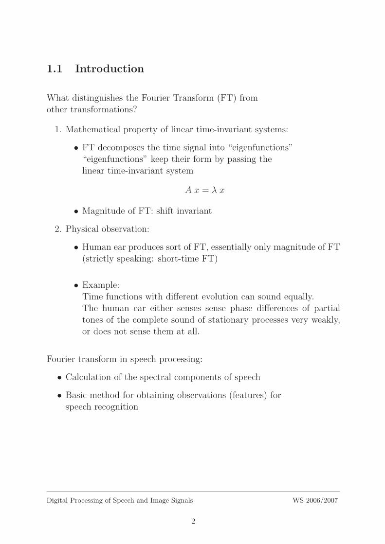
1.1 Introduction
What distinguishes the Fourier Transform (FT) fromother transformations?
1. Mathematical property of linear time-invariant systems:
• FT decomposes the time signal into “eigenfunctions”“eigenfunctions” keep their form by passing thelinear time-invariant system
A x = λ x
• Magnitude of FT: shift invariant
2. Physical observation:
• Human ear produces sort of FT, essentially only magnitude of FT(strictly speaking: short-time FT)
• Example:Time functions with different evolution can sound equally.The human ear either senses sense phase differences of partialtones of the complete sound of stationary processes very weakly,or does not sense them at all.
Fourier transform in speech processing:
• Calculation of the spectral components of speech
• Basic method for obtaining observations (features) forspeech recognition
Digital Processing of Speech and Image Signals WS 2006/2007
2

0
0
φ = 0
0
0
φ = π/2
0
0
random φ
Figure 1.1: Oscillograms of three timefunctions composed as sum of 20 partialoscillations. a) φn = 0, b) φn = π
2, c) φn
statistical.
0
Figure 1.2: Amplitude spectrum of a timefunction composed as sum of 20 partialtones.
Figure 1.3: from left to right: original photo, low-pass and high-pass filtered version
Digital Processing of Speech and Image Signals WS 2006/2007
3

amplitude spectrum
0
original signal
0
0
inverse FT for phase φ(f) = 0
0
0
Inverse FT for phase φ(f) = π2
0
0
Inverse FT for random phase φ(f)
0
0
Figure 1.4: Phase manipulation for portion of a speech signal (vowel ’o’) sampled at 8kHz,25ms analysis window (200 samples), 512 point FFT
Digital Processing of Speech and Image Signals WS 2006/2007
4

amplitude spectrum
0
original signal
0
0
inverse FT for phase φ(f) = 0
0
0
inverse FT for phase φ(f) = π2
0
0
inverse FT for random phase φ(f)
0
0
Figure 1.5: Phase manipulation for portion of a speech signal (consonant ’n’) sampled at8kHz, 25ms analysis window (200 samples), 512 point FFT
Digital Processing of Speech and Image Signals WS 2006/2007
5

amplitude spectrum
0
original signal
0
inverse FT for phase φ(f) = 0
0
0
inverse FT for phase φ(f) = π2
0
0
inverse FT for random phase φ(f)
0
0
Figure 1.6: Phase manipulation for a Heaviside–function (step–function)
Digital Processing of Speech and Image Signals WS 2006/2007
6

Why Fourier?
Roughly:
• Production, description and algorithmic operations on signals (func-tions or measurement curves over the time axis) can be described verywell in Fourier domain (frequency domain).
Deeper reason:
• Production, description and algorithmic operations on signals are largelybased on linear time-invariant (LTI) operations.
• Fourier Transform: simple representation of LTI-operations (later:convolution theorem)
Why continuous?
• Real world is continuous
• Computer (digital = time discrete = sampled)
model of the real world
Digital Processing of Speech and Image Signals WS 2006/2007
7
t
AT
glottal
pulsesvocal
tract
filter
radiation
from lips
and nose
t
T
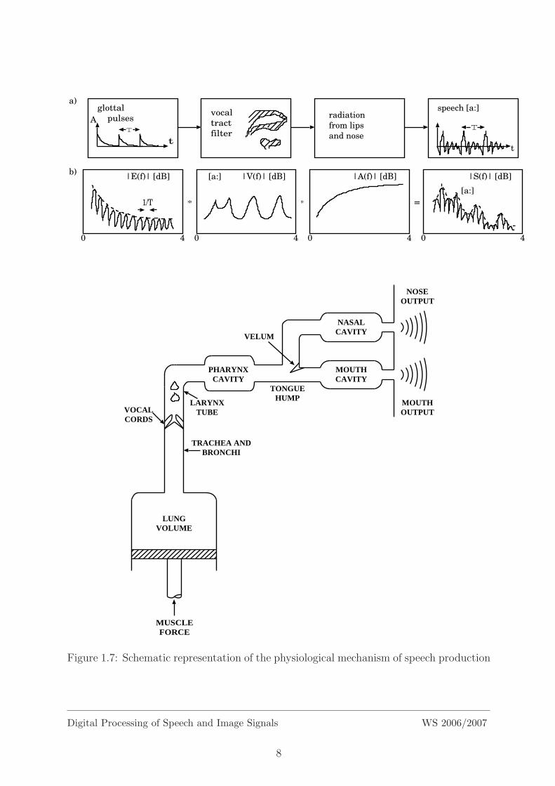
speech [a:]a)
b)
0 4 0 4 0 4 0 4
1/T
|E(f)| [dB] |V(f)| [dB][a:] |A(f)| [dB] |S(f)| [dB]
* * =
[a:]
MUSCLEFORCE
LUNGVOLUME
PHARYNXCAVITY
NASALCAVITY
MOUTHCAVITY
TONGUEHUMP
VELUM
VOCALCORDS
TRACHEA ANDBRONCHI
LARYNXTUBE
NOSEOUTPUT
MOUTHOUTPUT
Figure 1.7: Schematic representation of the physiological mechanism of speech production
Digital Processing of Speech and Image Signals WS 2006/2007
8

signal (speech, image)
feature extraction(signal analysis)
feature vector(pattern vector)
(pattern)comparison
decision
reference data(vectors, features)
Examples:
• Spoken language
• Written numbers (letters)
• Cell recognition (red blood cells)
Digital Processing of Speech and Image Signals WS 2006/2007
9

Examples of applications of Fourier Transform:
• Electrical switchgears
• Recognition and coding
– Speech and general acoustic signals
– Image signals
• Time series analysis:
– Astronomical measurement curves
– Stock-market course
– . . .
• Computer tomography
• Solving differential equations
• Description of image production in optical systems
Digital Processing of Speech and Image Signals WS 2006/2007
10

1.2 Linear time-invariant Systems
Example:
– speech production
– electrical systems
S
h(t)input signal
x(t)output signal
y(t)
symbolic:
t→ y(t) = S t→ x(t)
simplified:
y(t) = S x(t)
• Note: the complete time domain of the function is important, notindividual positions in time t.
more exact:
y = S x
LTI–System: (LTI = Linear Time-Invariant)
• Linear:
Additive:
S x1 + x2 = S x1+ S x2
Homogeneous:
S α x = αS x , α ∈ IR
• Time-invariant:
t→ y(t− t0) = S t→ x(t− t0) , t0 ∈ IR
Digital Processing of Speech and Image Signals WS 2006/2007
11

Mathematical theorem:
• Linearity and time invariance result in convolution representation
• Output signal y(t) of LTI system S with input signal x(t):
y(t) =
∞∫
−∞
x(t− τ) h(τ) dτ
=
∞∫
−∞
x(τ) h(t− τ) dτ
= x(t) ∗ h(t)
• h: impulse response of the system S
∆τ1/∆τ
∆τe (t)
t t
x (t)
τi
• system response h∆τ (t) to excitation e∆τ (t):
h∆τ(t) = S e∆τ(t)
• signal x(t) is represented as sum of amplitude weighted and timeshifted elementary functions e∆τ(t):
x(t) = lim∆τ→0
[∑
i
x(τi) e∆τ (t− τi) ∆τ
]
Digital Processing of Speech and Image Signals WS 2006/2007
12

Hence the following holds for the output signal y(t):
y(t) = S x(t)
= S
lim
∆τ→0
∑
i
x(τi) e∆τ(t− τi) ∆τ
= lim∆τ→0
[S
∑
i
x(τi) e∆τ (t− τi) ∆τ
]
additivity:
= lim∆τ→0
[∑
i
S x(τi) e∆τ(t− τi) ∆τ]
homogeneity (for x(τi) and ∆τ):
= lim∆τ→0
[∑
i
x(τi) S e∆τ (t− τi) ∆τ
]
time invariance:
= lim∆τ→0
[∑
i
x(τi) h∆τ (t− τi) ∆τ
]
limiting case ∆τ → 0 :
∑−→
∫
∆τ −→ dτ
τi −→ τ
h∆τ(t) −→ h(t)
result:
y(t) =
∞∫
−∞
x(τ) h(t− τ) dτ = x(t) ∗ h(t)
h(t): impulse response of the system
Digital Processing of Speech and Image Signals WS 2006/2007
13

Examples of LTI-operations:
• Oscillatory systems (electrical or mechanical) withexternal excitation:
x(t) −→ h(τ) −→ y(t)
y(t) =
∫h(t− τ) x(τ) dτ
y′′(t) + 2αy′(t) + β2y(t) = x(t)
α, β: parameters depending on the oscillatory system
• More general electrical engineering systems:
high-pass, low-pass, band-pass
• Sliding average value:
x(t) −→ S −→ y(t) := x(t)
x(t) =1
T
+T/2∫
−T/2
x(t+ τ) dτ
• Differentiator:
x(t) −→ S −→ y(t) := x′(t)
• Comb filter: ”hypothesized” period T
x(t) −→ S −→ y(t) := x(t)− x(t− T )
• In general: linear differential equations with coefficients ck and dl
∑k
cky(k)(t) =
∑l
dlx(l)(t)
[ + further constraints ]
Digital Processing of Speech and Image Signals WS 2006/2007
14

Example of a non-linear system:
system: y(t) = x2(t)
x(t) = A cos(βt)
=⇒ y(t) = A2 cos2(βt) =A2
2(1 + cos(2βt))
frequency doubling
Digital Processing of Speech and Image Signals WS 2006/2007
15

1.3 Fourier Transform
Sinusoidal oscillation:
x(t) = A sin ( ω t + ϕ )
amplitude A
phase / null phase ϕ
angular frequency ω = 2 π f
j2 = −1, j ∈ C
cos
sin
αα
α
Im
Re
1
1
complex representation: ej α = cos α + j sin α, α ∈ IR
cos α =ejα + e−jα
2and sin α =
ejα − e−jα2j
dimension:
DIM(ω) DIM(t) = 1
DIM(ω) =1
DIM(t)=
1
[sec]= [Hz]
Digital Processing of Speech and Image Signals WS 2006/2007
16

LTI-System
y(t) =
∞∫
−∞
x(t− τ)h(τ)dτ = x(t) ∗ h(t)
• Determine the following specific input signal:
x(t) = A ej(ωt+ϕ)
• For this input signal the output signal becomes:
y(t) =
∞∫
−∞
A ej(ω(t−τ)+ϕ)h(τ)dτ
= A ej(ωt+ϕ)
∞∫
−∞
h(τ)e−jωτdτ
︸ ︷︷ ︸H(ω) = F h(τ)
= x(t) · H(ω)
• Definition of the Fourier transform:
H(ω) =
∞∫
−∞
h(τ)e−jωτdτ = F h(τ) = F τ → h(τ)
(→ decomposition into e−jωτ)
• H(ω) is called transfer function of the system
Remark about x(t) = A ej(ωt+ϕ):
• The shape of the input signal x(t), i.e. its frequency ω (“eigenfunc-tion”) remains invariant
• Amplitude (intensity) and phase (time shift) are depending onH(ω) (“eigenvalue”)
(→ analogy to the problem of eigenvalues in linear algebra)
Digital Processing of Speech and Image Signals WS 2006/2007
17
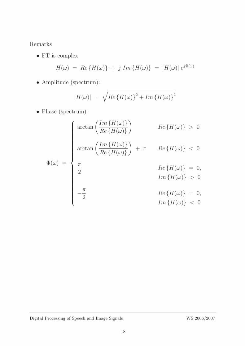
Remarks
• FT is complex:
H(ω) = Re H(ω) + j Im H(ω) = |H(ω)| ejΦ(ω)
• Amplitude (spectrum):
|H(ω)| =
√Re H(ω)2 + Im H(ω)2
• Phase (spectrum):
Φ(ω) =
arctan
(Im H(ω)Re H(ω)
)Re H(ω) > 0
arctan
(Im H(ω)Re H(ω)
)+ π Re H(ω) < 0
π
2Re H(ω) = 0,
Im H(ω) > 0
−π2
Re H(ω) = 0,
Im H(ω) < 0
Digital Processing of Speech and Image Signals WS 2006/2007
18

Examples of Fourier transforms:
1. Rectangle function
h(t) = rect(t
T) =
1, |t| ≤ T/20, |t| > T/2
H(ω) =
∞∫
−∞
h(t)e−jωtdt =
T2∫
−T2
e−jωtdt =1
−jω[e−jω
T2 − ejω T
2
]
=2
ωsin(
ωT
2) =
T sin(ωT
2)
ωT
2
(here: Im H(ω) = 0)
t
h(t)
H(ω)
ω
Digital Processing of Speech and Image Signals WS 2006/2007
19

2. Double-sided exponential
h(t) = e−α|t| with α > 0
H(ω) =
∞∫
−∞
h(t)e−jωtdt
=
∞∫
0
e−(α+jω)tdt+
∞∫
0
e−(α−jω)tdt
=
[e−(α+jω)t
−(α+ jω)+
e−(α−jω)t
−(α− jω)
]∞
0
= 0 + 0− 1
−(α+ jω)− 1
−(α− jω)
=α− jω + α+ jω
α2 + ω2
=2α
α2 + ω2
• Imaginary part equals 0
• Infinite spectrum
• No zeros
h(t)
t
H( )ω
ω
• If h(t) is symmetric (i.e. h(t) = h(−t)), imaginary parts drop awayand the real part is sufficient
Digital Processing of Speech and Image Signals WS 2006/2007
20

3. Damped oscillations
h(t) = e−α|t| cos(βt) with α > 0
H(ω) =
∞∫
−∞
h(t)e−jωtdt
=
∞∫
0
e−(α+jω)t cos(βt)dt+
∞∫
0
e−(α−jω)t cos(βt)dt
=
∞∫
0
e−(α+jω)t ejβt + e−jβt
2dt+
∞∫
0
e−(α−jω)t ejβt + e−jβt
2dt
= . . . (elementary calculation)
=α
α2 + (ω − β)2 +α
α2 + (ω + β)2
• Limiting case:
H(ω)|ω=±β =1
α+
α
α2 + (2β)2
=⇒ tends towards ∞ or −∞ if α tends towards 0
ω
H( )ω
β−β| |
h(t)
t
Digital Processing of Speech and Image Signals WS 2006/2007
21

4. Modulated rectangle function (“truncated cosine”)
h(t) =
cos(β t), |t| ≤ T/2
0, |t| > T/2
H(ω) =
∞∫
−∞
h(t)e−jωtdt
=
T2∫
−T2
cos(β t)e−jωtdt
= . . . (elementary calculation)
=T
2
sin
((ω − β)
T
2
)
(ω − β)T
2
+
sin
((ω + β)
T
2
)
(ω + β)T
2
| |
h(t)
t
H( )ω
ω
h(t)
t
| |
ω
ωH( )
β−β
Digital Processing of Speech and Image Signals WS 2006/2007
22

Fourier Transform pairs (u = ω/2π)
Rectangle function
1
-1/2 1/2
-1/2 1/2
Triangle function
1
Exponential function
e-α|x|
Gaussian function
e-αx2
Unit impulse
δ(x)
1
Sinc function
Squared sinc function
sin(πu)πu
1
α2+(2πu)2
2α
πu2
αe-πα
1
Digital Processing of Speech and Image Signals WS 2006/2007
23
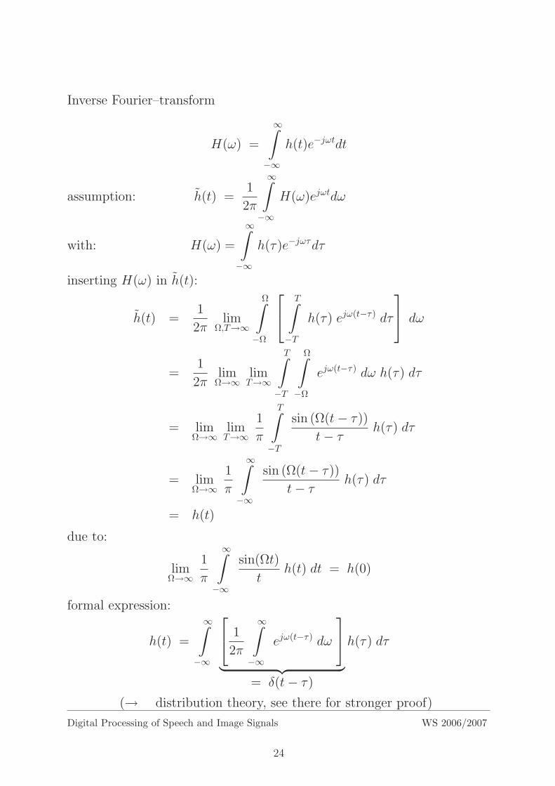
Inverse Fourier–transform
H(ω) =
∞∫
−∞
h(t)e−jωtdt
assumption: h(t) =1
2π
∞∫
−∞
H(ω)ejωtdω
with: H(ω) =
∞∫
−∞
h(τ)e−jωτdτ
inserting H(ω) in h(t):
h(t) =1
2πlim
Ω,T→∞
Ω∫
−Ω
T∫
−T
h(τ) ejω(t−τ) dτ
dω
=1
2πlim
Ω→∞limT→∞
T∫
−T
Ω∫
−Ω
ejω(t−τ) dω h(τ) dτ
= limΩ→∞
limT→∞
1
π
T∫
−T
sin (Ω(t− τ))t− τ h(τ) dτ
= limΩ→∞
1
π
∞∫
−∞
sin (Ω(t− τ))t− τ h(τ) dτ
= h(t)
due to:
limΩ→∞
1
π
∞∫
−∞
sin(Ωt)
th(t) dt = h(0)
formal expression:
h(t) =
∞∫
−∞
1
2π
∞∫
−∞
ejω(t−τ) dω
︸ ︷︷ ︸= δ(t− τ)
h(τ) dτ
(→ distribution theory, see there for stronger proof)
Digital Processing of Speech and Image Signals WS 2006/2007
24

1.4 Properties of the Fourier Transform
Symmetry
H(ω) =
∞∫
−∞
h(t) e−jωt dt = F h(t)
h(t) =1
2π
∞∫
−∞
H(ω) ejωt dω = F−1 H(ω)
F 2h(t) = FH(ω) = 2πh(−t)
F−1 Fh(t) = F−1H(ω) = h(t)
• Time domain and frequency domain are correlated symmetrically.
• Properties of FT are valid in both domains, especially the convolutiontheorem (see later).
Digital Processing of Speech and Image Signals WS 2006/2007
25

Theorems for the Fourier transform
H(ω) =
∞∫
−∞
e−jωt h(t) dt
consider the equation:
H(ω) = F h(t)
more exact:
ω → H(ω) = F t→ h(t)
1. Linearity: integral operator is linear
2. Inverse scaling, similarity principle:
∞∫
−∞
h(αt) e−jωt dt =1
|α|
∞∫
−∞
h(τ) e−jωατ dτ
Fh(αt) =1
|α| H(ω
α), α ∈ IR\0
Note:
Absolute value, because integral boundaries are swapped for α < 0.
3. Shift: h(t− t0)∞∫
−∞
h(t− t0) e−jωt dt = e−jωt0∞∫
−∞
h(t− t0) e−jω(t−t0) dt
= e−jωt0∞∫
−∞
h(τ) e−jωτ dτ
Digital Processing of Speech and Image Signals WS 2006/2007
26
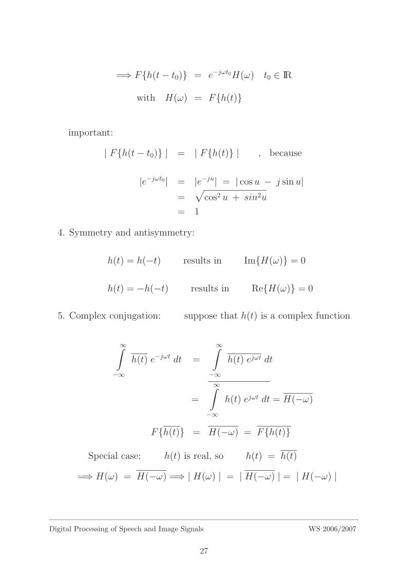
=⇒ Fh(t− t0) = e−jωt0H(ω) t0 ∈ IR
with H(ω) = Fh(t)
important:
| Fh(t− t0) | = | Fh(t) | , because
|e−jωt0| = |e−ju| = | cosu − j sinu|=
√cos2 u + sin2u
= 1
4. Symmetry and antisymmetry:
h(t) = h(−t) results in ImH(ω) = 0
h(t) = −h(−t) results in ReH(ω) = 0
5. Complex conjugation: suppose that h(t) is a complex function
∞∫
−∞
h(t) e−jωt dt =
∞∫
−∞
h(t) ejωt dt
=
∞∫
−∞
h(t) ejωt dt = H(−ω)
Fh(t) = H(−ω) = Fh(t)
Special case: h(t) is real, so h(t) = h(t)
=⇒ H(ω) = H(−ω) =⇒ | H(ω) | = | H(−ω) | = | H(−ω) |
Digital Processing of Speech and Image Signals WS 2006/2007
27

6. Differentiation:
dh
dt=
∂
∂t
1
2π
∞∫
−∞
H(ω) ejωt dω
=1
2π
∞∫
−∞
H(ω) jω ejωt dω
Fdh(t)dt = jω Fh(t)
Interpretation: differentiation = enhancement of high frequencies(due to the multiplication with ω)
7. Integration:
Ft∫
−∞
h(τ)dτ =1
jωFh(t)
Proof: similar to differentiation or inversion
8. Modulation principle:
Fh(t) cos(ω0t) =
∞∫
−∞
h(t) cos(ω0t) e−jωt dt
=1
2
∞∫
−∞
h(t) ejω0t e−jωt dt +
∞∫
−∞
h(t) e−jω0t e−jωt dt
=1
2
∞∫
−∞
h(t) e−j(ω−ω0)t dt +
∞∫
−∞
h(t) e−j(ω+ω0)t dt
=1
2[ H(ω − ω0) + H(ω + ω0) ]
and similarly
F h(t) sin(ω0t) =1
2j[ H(ω − ω0) − H(ω + ω0) ]
Digital Processing of Speech and Image Signals WS 2006/2007
28
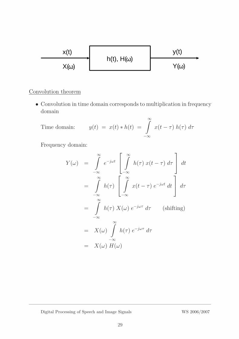
h(t), H(ω) x(t)
X(ω)
y(t)
Y(ω)
Convolution theorem
• Convolution in time domain corresponds to multiplication in frequencydomain
Time domain: y(t) = x(t) ∗ h(t) =
∞∫
−∞
x(t− τ) h(τ) dτ
Frequency domain:
Y (ω) =
∞∫
−∞
e−jωt
∞∫
−∞
h(τ) x(t− τ) dτ
dt
=
∞∫
−∞
h(τ)
∞∫
−∞
x(t− τ) e−jωt dt
dτ
=
∞∫
−∞
h(τ) X(ω) e−jωτ dτ (shifting)
= X(ω)
∞∫
−∞
h(τ) e−jωτ dτ
= X(ω) H(ω)
Digital Processing of Speech and Image Signals WS 2006/2007
29

• Likewise, multiplication in time domain corresponds to convolution infrequency domain (note the factor 1
2π):
Time domain: y(t) = a(t) · b(t)
Frequency domain:
Y (ω) =
∞∫
−∞
a(t) · b(t) e−jωt dt
=
∞∫
−∞
a(t)1
2π
∞∫
−∞
B(ω)ejωt e−jωt dω dt
=1
2π
∞∫
−∞
B(ω)
∞∫
−∞
a(t)e−j(ω−ω)t dt dω
=1
2π
∞∫
−∞
A(ω − ω) ·B(ω)dω
=1
2πA(ω) ∗B(ω)
• Motivation for the Fourier transform:FT gives the “simplest” representation of the system operation, be-cause every LTI-System can be interpreted as convolution of the inputsignal x(t) and the impulse response of the system h(t). Convolutioncan be then efficiently calculated using FT and convolution theorem.
• Mathematical: eigenfunctions
Digital Processing of Speech and Image Signals WS 2006/2007
30
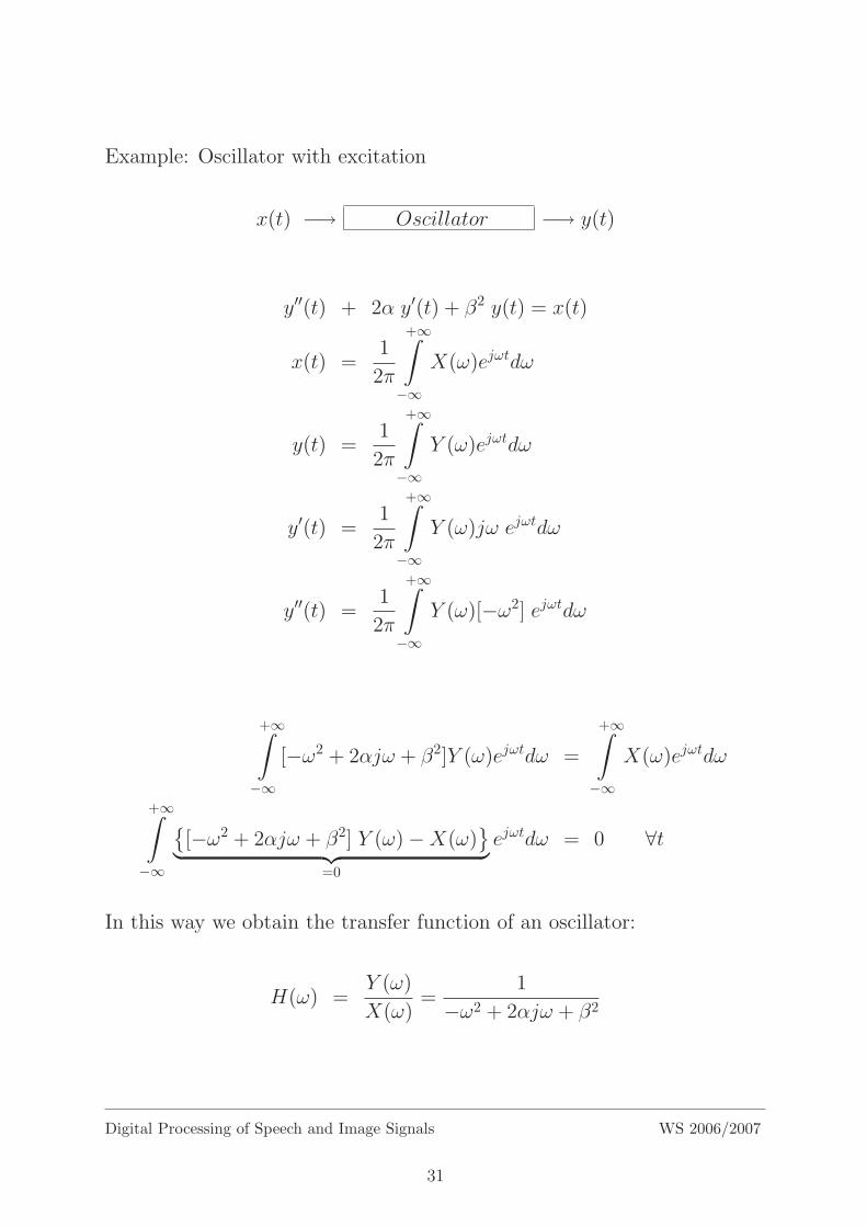
Example: Oscillator with excitation
x(t) −→ Oscillator −→ y(t)
y′′(t) + 2α y′(t) + β2 y(t) = x(t)
x(t) =1
2π
+∞∫
−∞
X(ω)ejωtdω
y(t) =1
2π
+∞∫
−∞
Y (ω)ejωtdω
y′(t) =1
2π
+∞∫
−∞
Y (ω)jω ejωtdω
y′′(t) =1
2π
+∞∫
−∞
Y (ω)[−ω2] ejωtdω
+∞∫
−∞
[−ω2 + 2αjω + β2]Y (ω)ejωtdω =
+∞∫
−∞
X(ω)ejωtdω
+∞∫
−∞
[−ω2 + 2αjω + β2] Y (ω)−X(ω)
︸ ︷︷ ︸
=0
ejωtdω = 0 ∀t
In this way we obtain the transfer function of an oscillator:
H(ω) =Y (ω)
X(ω)=
1
−ω2 + 2αjω + β2
Digital Processing of Speech and Image Signals WS 2006/2007
31

h(t) =1
2π
+∞∫
−∞
H(ω)ejωtdω
(can be given explicitly)
y(t) =
+∞∫
−∞
x(t) h(t− τ)dτ
Note:y(t) does not contain the component which corresponds to the homoge-neous differential equation of the oscillator.
FourierTransform
Convolution with h(t)
Multiplication with H(ω) = Fh(t)
Inverse FourierTransform
x(t)
X(ω)
y(t)
Y(ω)
Digital Processing of Speech and Image Signals WS 2006/2007
32

1.5 Parseval Theorem
Convolution theorem:
F−1 H(ω) X(ω) =
∞∫
−∞
h(t) x(τ − t) dt
(⋆)1
2π
∞∫
−∞
H(ω) X(ω) ejωτ dω = (h ∗ x) (τ)
We make two special assumptions:
i) x(−t) := h(t), then: X(ω) = H(ω)
ii) τ = 0
Inserting in (⋆) results in:
1
2π
∞∫
−∞
H(ω)H(ω) dω =
∞∫
−∞
h(t)h(t) dt
1
2π
∞∫
−∞
|H(ω)|2 dω =
∞∫
−∞
|h(t)|2 dt = E
• Energy E in time domain = Energy E in frequency domain
(up to the factor1
2π; aid: use normalization factor
1√2π
for both
directions of Fourier Transform)
• Physical aspect: energy conservation
• Mathematical aspect: unitary (orthogonal) representation in vectorspace
• |H(ω)|2 is called power spectral density.
Digital Processing of Speech and Image Signals WS 2006/2007
33

1.6 Autocorrelation Function
Autocorrelation function
• Autocorrelation function of time continuoussignal or function h(t) is defined as:
R(t) =
∞∫
−∞
h(τ) h(t+ τ)dτ
• The following equation is valid:
R(t) = h(t) ∗ h(−t) → which results in R(t) = R(−t)
• Fourier transform gives: (”Wiener-Khinchin Theorem”)
FR(t) = H(ω) H(ω) = |H(ω)|2
• Thus: Fourier transform connects autocorrelationfunction R(t) and power spectral density |H(ω)|2
|H(ω)|2 =
∞∫
−∞
R(t) e−jωt dt =
∞∫
−∞
R(t) cos(ωt) dt
• Remark:autocorrelation is a special case of the cross correlation between sig-nals x(τ) and h(t)
Ch,x =
∞∫
−∞
h(τ) x(t+ τ)dτ
Digital Processing of Speech and Image Signals WS 2006/2007
34

1.7 Existence of the Fourier Transform
Conditions for h(t) for the existence of the Fourier transform
H(ω) =
∞∫
−∞
e−jωt h(t) dt , h(t) =1
2π
∞∫
−∞
ejωt H(ω) dω
When are those equations valid?
Sufficient conditions:
1. h(t) is absolutely integrable:
∞∫
−∞
|h(t)|dt <∞
2. h(t) has finite number of jumps, minima and maxima in each intervalof IR
3. h(t) has no infinite jumps
More general conditions are possible (but rather complex set of conditions):
• Generalized functions, distributions,definition as functional
• Example: δ-function:
∞∫
−∞
δ(t) h(t) dt = h(0) for all functions h
Digital Processing of Speech and Image Signals WS 2006/2007
35
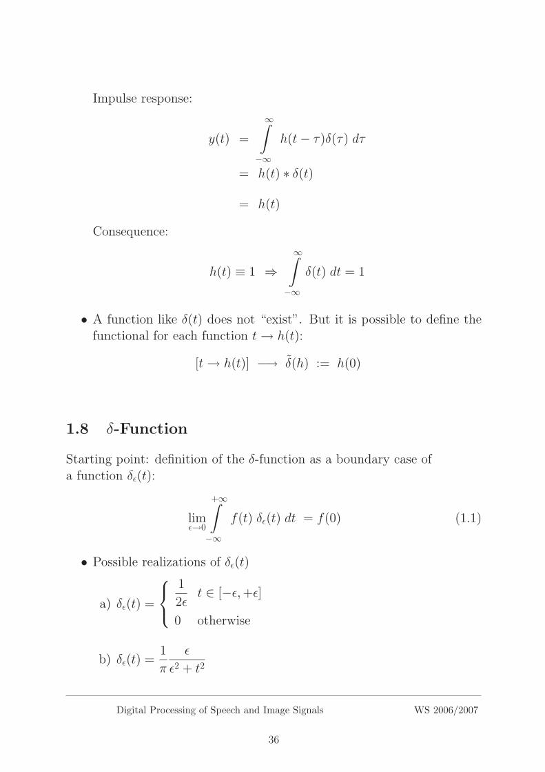
Impulse response:
y(t) =
∞∫
−∞
h(t− τ)δ(τ) dτ
= h(t) ∗ δ(t)
= h(t)
Consequence:
h(t) ≡ 1 ⇒∞∫
−∞
δ(t) dt = 1
• A function like δ(t) does not “exist”. But it is possible to define thefunctional for each function t→ h(t):
[t→ h(t)] −→ δ(h) := h(0)
1.8 δ-Function
Starting point: definition of the δ-function as a boundary case ofa function δǫ(t):
limǫ→0
+∞∫
−∞
f(t) δǫ(t) dt = f(0) (1.1)
• Possible realizations of δǫ(t)
a) δǫ(t) =
1
2ǫt ∈ [−ǫ,+ǫ]
0 otherwise
b) δǫ(t) =1
π
ǫ
ǫ2 + t2
Digital Processing of Speech and Image Signals WS 2006/2007
36

c) δǫ(t) =1
π
sin (t/ǫ)
t
d) δǫ(t) =1√2πǫ2
e−t2
2ǫ2
• During inversion of the Fourier transform we have “formally” ob-tained:
δ(t) =1
2π
+∞∫
−∞
ejωt dω = limΩ→∞
1
π
sin (Ωt)
t(1.2)
Fourier transform Fδ(t):
Fδ(t) =
+∞∫
−∞
e−jωtδ(t) dt
due to (1.1) the following holds:
Fδ(t) = ejωt|t=0 = 1
• Another derivation using (1.2):
δ(t) =1
2π
+∞∫
−∞
ejωt Fδ(t) dω general
=1
2π
+∞∫
−∞
ejωt dω according to (1.2)
Comparison results in:
Fδ(t) = 1
Digital Processing of Speech and Image Signals WS 2006/2007
37
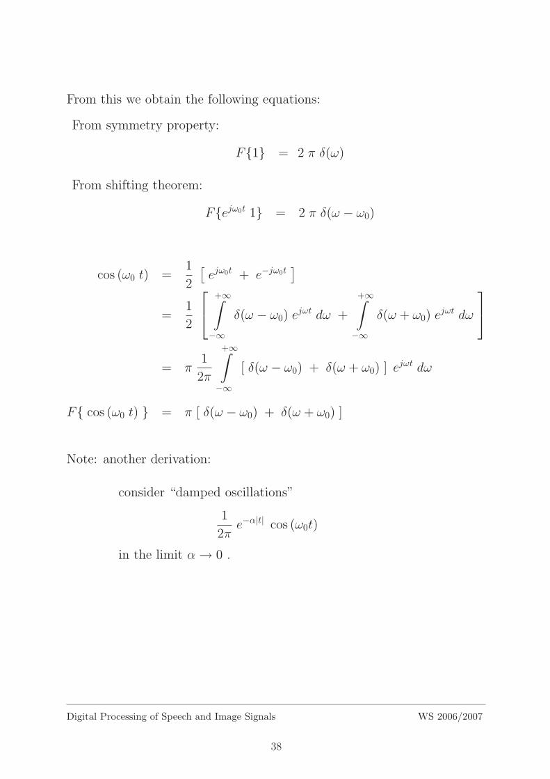
From this we obtain the following equations:
From symmetry property:
F1 = 2 π δ(ω)
From shifting theorem:
Fejω0t 1 = 2 π δ(ω − ω0)
cos (ω0 t) =1
2
[ejω0t + e−jω0t
]
=1
2
+∞∫
−∞
δ(ω − ω0) ejωt dω +
+∞∫
−∞
δ(ω + ω0) ejωt dω
= π1
2π
+∞∫
−∞
[ δ(ω − ω0) + δ(ω + ω0) ] ejωt dω
F cos (ω0 t) = π [ δ(ω − ω0) + δ(ω + ω0) ]
Note: another derivation:
consider “damped oscillations”
1
2πe−α|t| cos (ω0t)
in the limit α→ 0 .
Digital Processing of Speech and Image Signals WS 2006/2007
38

Comb function
• define “comb function” (pulse train, sequence of δ-impulses):
x(t) =+∞∑
n=−∞δ(t− nT )
• Fourier transform of comb function:
X(ω) =
+∞∫
−∞
x(t) e−jωt dt
=
+∞∫
−∞
+∞∑
n=−∞δ(t− nT ) e−jωt dt
=+∞∑
n=−∞
+∞∫
−∞
δ(t− nT ) e−jωt dt
=+∞∑
n=−∞e−jωnT
= . . . (see Papoulis 1962, p. 44)
=2π
T
+∞∑
n=−∞δ(ω − n2π
T)
• in words:
δ-impulse sequence with period T in time domain
produces
δ-impulse sequence with period 1T in frequency domain
(i.e. 2πT in ω-frequency domain)
comb function is transformed to comb function
Digital Processing of Speech and Image Signals WS 2006/2007
39
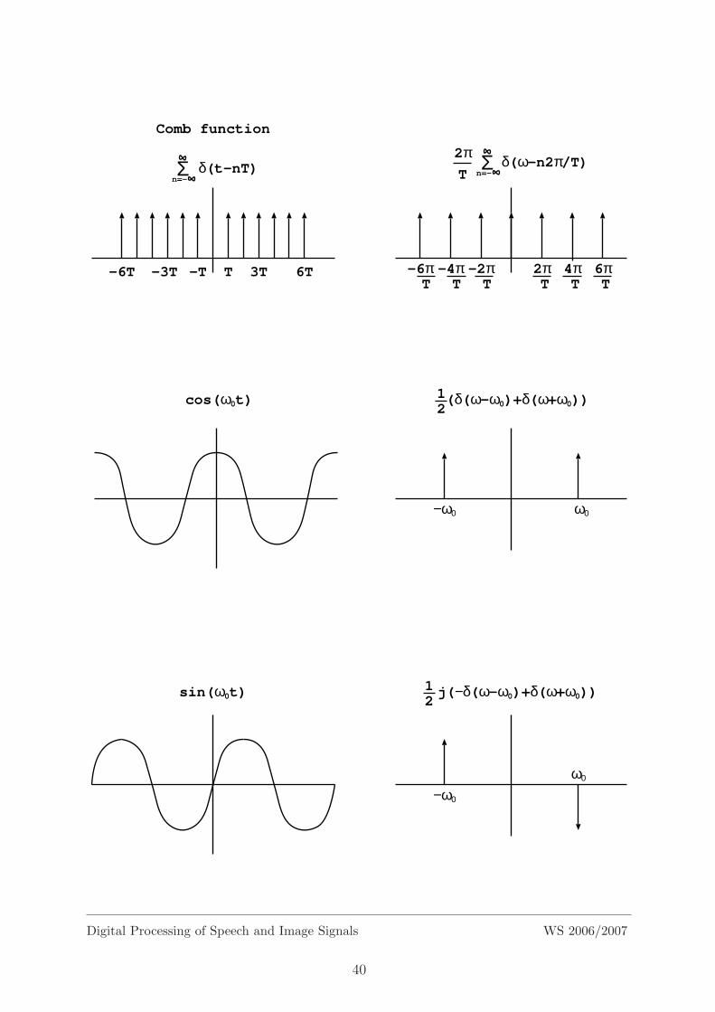
Comb function
cos(ω0t)
sin(ω0t)
-2π-4π-6π 2π 4π 6πT T T T T T
T 3T-T-3T 6T-6T
δ(t-nT)Σn=-
12j(−δ(ω-ω0)+δ(ω+ω0))
(δ(ω-ω0)+δ(ω+ω0))12
Σ δ(ω-n2π/T)n=-
2πT
−ω0 ω0
−ω0
ω0
Digital Processing of Speech and Image Signals WS 2006/2007
40

1.9 Motivation for Fourier Series
x : IR −→ IR
t −→ x(t)
Consider a periodical function x with period T :
x(t) = x(t+ T ) for each t ∈ IR
then also x(t) = x(t+ kT ) for k ∈ Z
Examples:
• Constant function:
x0(t) = A0
• Harmonic oscillator:
x1(t) = A1 cos (2π
Tt + ϕ1) , A1 > 0
• All higher harmonic:
xn(t) = An cos (n2π
Tt + ϕn) , An > 0
therefore
x(t) =∞∑
n=0
An cos (n ω0 t + ϕn) with ω0 =2 π
T, An ≥ 0
is periodical with period T = 2πω0
• Another notation:
x(t) =∞∑
n=−∞Bn e
−j n ω0 t where Bn is a complex number
Digital Processing of Speech and Image Signals WS 2006/2007
41
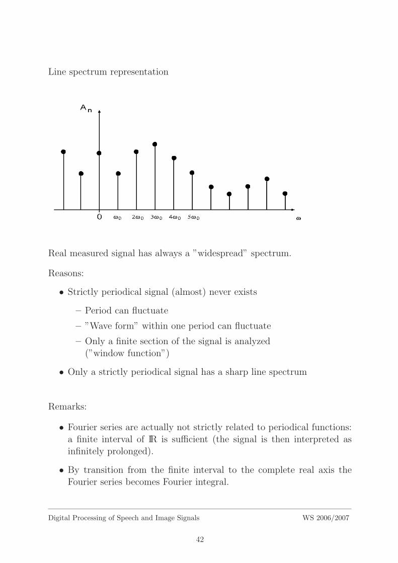
Line spectrum representation
Real measured signal has always a ”widespread” spectrum.
Reasons:
• Strictly periodical signal (almost) never exists
– Period can fluctuate
– ”Wave form” within one period can fluctuate
– Only a finite section of the signal is analyzed(”window function”)
• Only a strictly periodical signal has a sharp line spectrum
Remarks:
• Fourier series are actually not strictly related to periodical functions:a finite interval of IR is sufficient (the signal is then interpreted asinfinitely prolonged).
• By transition from the finite interval to the complete real axis theFourier series becomes Fourier integral.
Digital Processing of Speech and Image Signals WS 2006/2007
42

Calculation of Fourier coefficients:
• Consider a periodical function x(t) with period T = 2πω0
• approach:
x(t) =+∞∑
n=−∞an e
j nω0 t a ∈ C
• multiplication with e−j mω0 t where m ∈ IN and integration over oneperiod result in:
+T/2∫
−T/2
x(t) e−j m ω0 t dt =+∞∑
n=−∞an
+T/2∫
−T/2
ej (n−m) ω0 t dt
• Due to “orthogonality” holds:
+T/2∫
−T/2
ej (n−m) ω0 t dt =
T if n = m
0 if n 6= m
• Then:
T/2∫
−T/2
x(t) e−j m ω0 t dt = am T
• Result:
an =1
T
+T/2∫
−T/2
x(t) e−j n ω0 t dt
=1
T
+T/2∫
−T/2
x(t) cos (n ω0 t) dt − j1
T
+T/2∫
−T/2
x(t) sin (n ω0 t) dt
Digital Processing of Speech and Image Signals WS 2006/2007
43

Spectrum of a periodical function
• If x(t) is periodical with the period T = 2πω0
, then
x(t) =+∞∑
n=−∞an e
j nω0 t, an ∈ C
• The Fourier transform X(ω) is:
X(ω) = Fx(t)
=+∞∑
n=−∞an Fej n ω0 t︸ ︷︷ ︸
= 2πδ(ω − nω0)
= 2 π+∞∑
n=−∞an δ(ω − nω0)
• Note:
This derivation is formal, because the Fourier integral does notexist in the “usual sense”;strict derivation within the scope of distribution theory.
• In words:
a periodic function with the period T has a Fourier transform in theform of a line spectrum with the distance ω0 = 2π
T between the com-ponents.
Digital Processing of Speech and Image Signals WS 2006/2007
44

1.10 Time Duration and Band Width
1. Similarity principle:
Fh(αt) =1
|α| H(ω
α)
t
h( t)α0<α<1:
h(t)
t
1 H( )_ _α α
ω
ω
H( )
ω
ω
time duration T band width B
T · B = const.
• High resolution in the time domain results in low resolution in thefrequency domain and vice versa
Digital Processing of Speech and Image Signals WS 2006/2007
45

2. Special case: h(t) with
Im H(ω) = 0 ( h(t) symmetrical )
and
Re H(ω) ≥ 0
h(t) has maximum for t = 0:
h(t) =1
2π
∞∫
−∞
H(ω) cos(ωt) dω ≤ 1
2π
∞∫
−∞
H(ω) dω = h(0)
define:
T =1
h(0)
∞∫
−∞
h(t) dt
B =1
H(0)
∞∫
−∞
H(ω) dω
from
T =H(0)
h(0)and B = 2 π
h(0)
H(0)
follows
T · B = 2 π
Digital Processing of Speech and Image Signals WS 2006/2007
46

3. In general: normalized impulse h(t) ∈ IR with∞∫
−∞
h2(t) dt = 1, h(t) ∈ IR
T 2 :=
∞∫
−∞
h2(t) t2 dt
B2 :=
∞∫
−∞
|H(ω) |2 ω2 dω
= 2 π
∞∫
−∞
[h′(t)]2dt
• Results in “uncertainty relation”:
T · B ≥√π
2
• Proof: Cauchy-Schwarz inequality
| xT y | ≤ ||x|| · ||y||
∣∣∣∣∣∣
∞∫
−∞
[ t h(t) ] h′(t) dt
∣∣∣∣∣∣
2
︸ ︷︷ ︸=1
4
≤∞∫
−∞
[ t h(t)]2 dt
︸ ︷︷ ︸= T 2
∞∫
−∞
[ h′(t) ]2dt
︸ ︷︷ ︸B2
2πFrom: partial integration
∫u′(t) v(t) dt = u(t) v(t)−
∫u(t) v′(t) dt
∫[ h(t) h′(t) ]︸ ︷︷ ︸
u′(t)
t︸︷︷︸v(t)
dt =1
2h(t)2 t −
∫1
2h2(t) 1 dt
∞∫
−∞
[ h(t) h′(t) ] t dt = 0 − 1
2
Digital Processing of Speech and Image Signals WS 2006/2007
47

Equality sign is valid for linear dependency:
h′(t) = −λ t h(t)dh
h= −λ t dt
log(h) = −1
2λ t2 + const., λ > 0
=⇒ Optimum T · B =
√π
2for Gauss’ impulse
h(t) =λ√2π
e−1
2λ t2
Variance: σ2 =1
λ
Quantum Physics: similar statement about position and impulseof a particle
Digital Processing of Speech and Image Signals WS 2006/2007
48

4. Finite positive signal
g(t)
≥ 0 0 ≤ t ≤ T= 0 t < 0 or T < t
0 T
g(t)
t
The following is valid for the amplitude spectrum |G(ω)|:
|G(ω)| =
∣∣∣∣∣∣
+∞∫
−∞
g(t) e−jωtdt
∣∣∣∣∣∣
≤+∞∫
−∞
|g(t)| |e−jωt|dt
=
+∞∫
−∞
|g(t)| dt
because g(t) ≥ 0
= G(0)
Define the band width ωB as:
|G(ωB)|2 =G2(0)
2and |G(ωB)|2 ≤ |G(ω)|2 for |ω| < ωB
Then:
T ωB ≥π
2
Digital Processing of Speech and Image Signals WS 2006/2007
49

Proof:
The following inequalities are valid:
a2 + b2 ≥ (a− b)2
2∀ a, b ∈ IR
| sinα|+ | cosα| ≥ 1 ∀ α ∈ IR
For the Fourier-Transform of g(t) holds:
ReG(ω) =
T∫
0
g(t) cosωt dt
ImG(ω) = −T∫
0
g(t) sinωt dt
For 0 ≤ ω t ≤ π
2holds: cosωt ≥ 0, sinωt ≥ 0
and therefore: cosωt+ sinωt = | cosωt|+ | sinωt| ≥ 1
ReG(ω) − ImG(ω) =
T∫
0
g(t) [cosωt+ sinωt] dt
≥T∫
0
g(t) 1 dt
= G(0)
|G(ω)|2 = Re2G(ω)+ Im2G(ω)
≥ [ReG(ω) − ImG(ω)]22
≥ 1
2G2(0) ≡ |G(ωB)|2
Digital Processing of Speech and Image Signals WS 2006/2007
50

Chapter 2
Discrete Time Systems
• Overview:
2.1 Motivation and Goal
2.2 Digital Simulation using Discrete Time Systems
2.3 Examples of Discrete Time Systems
2.4 Sampling Theorem and Reconstruction
2.5 Logarithmic Scale and dB
2.6 Quantization
2.7 Fourier Transform and z–Transform
2.8 System Representation and Examples
2.9 Discrete Time Signal Fourier Transform Theorems
2.10 Discrete Fourier Transform (DFT)
2.11 DFT as Matrix Operation
2.12 From continuous FT to Matrix Representation of DFT
2.13 Frequency Resolution and Zero Padding
2.14 Finite Convolution
2.15 Fast Fourier Transform (FFT)
2.16 FFT Implementation
Digital Processing of Speech and Image Signals WS 2006/2007
51

2.1 Motivation and Goal
If we want to process a continuous time signal x(t) with a computer, wehave to sample it at discrete equidistant time points
tn = n · TSwhere TS is called sampling period.
Terminology:“time discrete” is often called “digital”, where this adjective often(but not always) denotes the amplitude quantization,i.e. the quantization of the value x(n · TS).
Advantages of digital processing in comparison to analog components:
• independent of analog components and technical difficulties with re-spect to their realization;
• in principle arbitrary high accuracy;
• also non-linear methods are possible,in principle even every mathematical method.
Digital Processing of Speech and Image Signals WS 2006/2007
52

2.2 Digital Simulation using Discrete Time Systems
Task definition:
• Given:Analog system with input signal x(t) and output signal y(t);Sampling with sampling period TS
• Wanted:Discrete System with input signal x[n] and output signal y[n], suchthat
x[n] = x(nTS)
results in
y[n] = y(nTS)
• For which signals is such a digital simulation possible?
• The sampling theorem gives (most of) the answer.
Digital Processing of Speech and Image Signals WS 2006/2007
53

LTI System (analog to continuous time case):
• Linearity:
Homogeneity:
S α x[n] = α S x[n]
Additivity:
S x1[n] + x2[n] = S x1[n] + S x2[n]
• Shift invariance:
S x[n − n0] = y[n− n0], n0 whole number
Digital Processing of Speech and Image Signals WS 2006/2007
54

Representation of an LTI System as discrete convolution:
Unit impulse:
δ[n] =
1, n = 00, n 6= 0
The signal x[n] is represented with amplitude weighted and time shiftedunit impulses δ[n]. The system reacts on δ[n] with h[n]:
h[n] = S δ[n]
Input signal:
x[n] =∞∑
k=−∞x[k] δ[n− k]
Output signal:
y[n] = S
∞∑
k=−∞x[k] δ[n− k]
Additivity
=∞∑
k=−∞S x[k] δ[n− k]
Homogeneity
=∞∑
k=−∞x[k] S δ[n− k]
Time invariance
=∞∑
k=−∞x[k] h[n− k]
Input signal x[n] and output signal y[n] of a discrete time LTI system arelinked through discrete convolution.h[n] is called impulse response like in continuous time case.
Digital Processing of Speech and Image Signals WS 2006/2007
55

2.3 Examples of Discrete Time Systems
• Difference calculation:
y[n] = x[n] − x[n− n0]
• “1-2-1”-averaging:
y[n] = 0.5 · x[n− 1] + x[n] + 0.5 · x[n+ 1]
• sliding window averaging (“smoothing”)
y[n] =1
2M + 1
M∑
k=−Mx[n− k]
• weighted averaging: instead of constant weight
h[n] =1
2M + 1
arbitrary weights can be used:
y[n] =M∑
k=−Mh[k] · x[n− k]
Note: the only difference from general case isfinite length of the convolution kernel h[n].
• First order difference equation:(recursive averaging, averaging with memory)
y[n]− α y[n− 1] = x[n]
• (Digital) resonator (second order difference equation)
y[n]− α y[n− 1]− β y[n− 2] = x[n]
• Image processing:Gradient calculation and image enhancement(Roberts Operator, Laplace Operator)
Digital Processing of Speech and Image Signals WS 2006/2007
56

• Roberts Cross Operator
gray values x[i, j]
i i+1
j
j+1
2
|∇x[i, j]|2 = (x[i, j]− x[i+ 1, j + 1])2 + (x[i, j + 1]− x[i+ 1, j])2
Note: non-linear operation
simplified:
|∇x[i, j]| = |x[i, j]− x[i+ 1, j + 1]|+ |x[i, j + 1]− x[i+ 1, j]|
Digital Processing of Speech and Image Signals WS 2006/2007
57

Figure 2.1: Digital photo
Figure 2.2: Gradient image
Digital Processing of Speech and Image Signals WS 2006/2007
58

• Laplace Operator ≡ discrete approximation of the second derivation
∇2x[i, j] = 2ix[i, j] +2
jx[i, j]
= x[i+ 1, j]− 2x[i, j] + x[i− 1, j] +
x[i, j + 1]− 2x[i, j] + x[i, j − 1]
= x[i+ 1, j] + x[i− 1, j] + x[i, j + 1] + x[i, j − 1]− 4x[i, j]
1 -2 1
1
1
1
1
1
1-4
-2 i-1 i i+1
j+1
j
j-1
Image enhancement:
y[i, j] = x[i, j]−∇2x[i, j]
= h[i, j] ∗ x[i, j]
Digital Processing of Speech and Image Signals WS 2006/2007
59

Figure 2.3: Several real cases of Laplace Operator subtraction from original image. a)Original image b) Original image minus Laplace Operator (negative values are set to 0and values above the grey scale are set to the highest grade of grey)
Digital Processing of Speech and Image Signals WS 2006/2007
60

2.4 Sampling Theorem (Nyquist Theorem) and Re-
construction
The following will be analyzed and derived respectively:
How should we choose the sampling period TS, if we want to represent acontinuous signal x(t) with its sample values x(nTS) so that the signal x(t)can be exactly reconstructed from its sample values?
• Fourier transform of the continuous time signal x(t):
X(ω) = F x(t) =
∞∫
−∞
x(t) e−jωt dt
x(t) = F−1 X(ω) =1
2π
∞∫
−∞
X(ω) ejωt dω (2.1)
• Signal x(t) has limited bandwidth with upper limit ωB, which means:X(ω) = 0 for all |ω| ≥ ωBNote: X(ωB) = 0
• X(ω) in domain −ωB < ω < ωB can be represented as Fourier Series:
X(ω) =∞∑
n=−∞an exp(−jnπ ω
ωB) (2.2)
• The coefficients an are given by:
an =1
2ωB
ωB∫
−ωB
X(ω) exp(jnπω
ωB) dω (2.3)
• Comparison of the equations (2.1) and (2.3) shows that the coefficientsan are given by the values of the inverse Fourier transform of x(t) atpoints
tn =nπ
ωB(2.4)
The band limitation of X(ω) has to be considered for the integrationlimits in (2.1). Result:
an = x(nπ
ωB) · πωB
(2.5)
Digital Processing of Speech and Image Signals WS 2006/2007
61

• Inserting Eq. (2.5) into Eq. (2.2) and then in Eq. (2.1) results in:
x(t) =1
2π
ωB∫
−ωB
π
ωB
∞∑
n=−∞x(nπ
ωB) exp(−jnπ ω
ωB) exp(jωt) dω
• After swapping summation and integration and subsequent integra-tion:
x(t) =∞∑
n=−∞x(nπ
ωB)
sin(ωB (t− nπ
ωB))
ωB (t− nπ
ωB)
• Reconstruction of the signal x(t) from sample values is possible if
equidistant sample values x(nπ
ωB) = x(n · Ts) have the distance TS
TS =π
ωB(2.6)
• The sampling period TS corresponds to the sampling frequency ΩS:
ΩS =2π
TS
• Equation (2.6) shows that if the sampling frequency is
ΩS := 2 ωB
the original signal x(t) can be reconstructed exactly.
• In the Fourier series representation of X(ω) in equation (2.2), theperiod 2 · ωB has been supposed.ωB is the highest frequency component of the signal x(t).
Digital Processing of Speech and Image Signals WS 2006/2007
62

• Since X(ω) is equal to zero for |ω| ≥ ωB, the period 2 · ωB can besubstituted with every period 2 · ωB where ωB ≥ ωB. The previousderivation is also valid for this ωB.
• When
ωB =π
TS
then:
x(t) =∞∑
n=−∞x(nTS)
sin(π (t − nTS)/TS)
π (t − nTS)/TS
(reconstruction formula)
Note: limt→0sin(t)t = 1 (l’Hopital’s rule)
• The condition ωB ≥ ωB results in:
TS ≤π
ωB(2.7)
for the sampling period TS and in:
ΩS ≥ 2 · ωB (2.8)
for the sampling frequency ΩS.
• The equations (2.7) and (2.8) are denoted as sampling theorem. Thesampling frequency has to be at least twice as high as the upper limitfrequency of the signal ωB where X(ω) = 0 for |ω| ≥ ωB. If and onlyif this condition is satisfied, an exact reconstruction (without approx-imation) of a continuous signal x(t) from its sample values x(nTS) ispossible.
• Note: The sampling frequency ΩS = 2 · ωB is also calledNyquist frequency.
Digital Processing of Speech and Image Signals WS 2006/2007
63

t
x(t)
t
xs(t)
xr(t)
T
T
a)
b)
c)
Figure 2.4: Ideal reconstruction of a band-limited signal (from Oppenheim, Schafer)a) original signal b) sampled signal c) reconstructed signal
Digital Processing of Speech and Image Signals WS 2006/2007
64

X(ω)
ωωΒ−ωΒ
a)
ωωΒ−ωΒ
b)
-ΩS ΩS
. . . . . .
XS1(ω) ΩS > 2ωΒ,
XS2(ω)
ωωΒ−ωΒ
c)
, ΩS = 2ωΒ
-ΩS ΩS
. . . . . .
(Nyquist rate)
XS3(ω)
ωΒ−ωΒ
, ΩS < 2ωΒ (aliasing)
. . . . . .
ΩS−ΩS
d)
ω
Figure 2.5: Sampling of band-limited signal with different sampling rates:b) sampling rate higher than Nyquist rate - exact reconstruction possiblec) sampling rate equal to Nyquist rate - exact reconstruction possibled) sampling rate smaller than Nyquist rate - aliasing - exact reconstruction not possible
Digital Processing of Speech and Image Signals WS 2006/2007
65

Another proof using delta- and comb-function:
Sampling of the continuous signal x(t) with ΩS = 2πTS
• Band limitation: X(ω) = 0 for |ω| ≥ ωB
(always possible: analog to low-pass with T (ω) = 0 for |ω| ≥ ωB)
• Sampling procedure
Multiplication of a function with a comb-function in time domain
xs(t) = Ts x(t) ·+∞∑
n=−∞δ(t− nTs)
results in a convolution with a comb-function in frequency domain:
Xs(ω) = Ts ·1
2πX(ω) ∗ 2π
Ts
+∞∑
n=−∞δ
(ω − ω2πn
Ts
)
=
+∞∫
−∞
X(ω)+∞∑
n=−∞δ
(ω − ω2πn
Ts
)dω
=+∞∑
n=−∞X
(ω − n2π
Ts
)
=⇒ sampled signal has periodical Fourier spectrum
(Analogy to Fourier series: periodical signal has line spectrum, i.e.discrete spectrum)
No overlap if:
ωB ≤ ΩS − ωB2ωB ≤ ΩS
Digital Processing of Speech and Image Signals WS 2006/2007
66

• In so-called digital simulation, the signal x(t) is represented by itssampled values x(n · TS) measured at equidistant time points withdistance TS. With a proper sampling period TS an exact reconstruc-tion of the signal x(t) from the sampled values x(n · TS) is possible.
• If it is possible to exactly reconstruct the signal x(t) from the sampledvalues x(n·TS), then it is possible to perform a discrete time processingof the sampled values x(n · TS) on a computer, which is equivalent tothe continuous time processing of the signal x(t) (digital simulation).
• Continuous time processing:
y(t) =
∞∫
−∞
x(τ) h(t− τ) dτ
• Discrete time processing:
– Sampling period TS
– x[n] := x(nTS)
y(nTS) =∞∑
k=−∞x(kTS) h(nTS − kTS) TS, h[n] = h(nTS)
y[n] =∞∑
k=−∞x[k] h[n− k]
• As a result of the convolution theorem (convolution in time domaincorresponds to multiplication in frequency domain), the band limitedinput signal gives an also band limited output signal which is exactlydetermined by its sampled values.
Digital Processing of Speech and Image Signals WS 2006/2007
67

Important:
• In the domain |ω| < ΩS/2 the Fourier transform of a continuous timesignal x(t) is identical with the Fourier–transform of the correspondingsampled discrete time signal x(nTS):
X(ω) =
∞∫
−∞
x(t) exp(−jωt) dt
for |ω| ≤ ΩS/2 is identical to
TS ·XS(ω) = TS ·∞∑
n=−∞x(nTS) exp(−jωTSn)
= TS ·∞∑
n=−∞x(nTS) exp(−j2πω
ΩSn)
• Inverse Fourier transform of discrete time signal:
x(nTS) =1
ΩS
ΩS/2∫
−ΩS/2
XS(ω) exp(jωTSn) dω
• One period:
−ΩS
2≤ ω ≤ ΩS
2
−π ≤ 2πω
ΩS≤ π
• The Fourier transform of a discrete time signal is periodic in ω withthe period 2π/TS = ΩS.
• The Fourier transform of a discrete time signal iscontinuous in ω.
Digital Processing of Speech and Image Signals WS 2006/2007
68

Frequency normalization
• Define the normalized frequency ωN :
ωN : = 2πω
ΩS
• Definition: (ω now denotes a normalized frequency)
– Fourier transform of discrete time signal x[n]:
X(ejω) =+∞∑
n=−∞x[n] exp(−jωn)
Note the notation X(ejω).
– Inverse Fourier transform of discrete time signal x[n]:
x[n] =1
2π
π∫
−π
X(ejω) exp(jωn) dω
Digital Processing of Speech and Image Signals WS 2006/2007
69

2.5 Logarithmic Scale and dB
Why?
– large dynamic range for the amplitude values of a signal
x(t) = A cos βt
A := amplitude(pressure, velocity, inclination, current, voltage, ... )“linear” variable
A0 := reference amplitudepredefined value for calibration
dB := “decibel”
A[dB] ≡ 20 · lg A
A0, lg ≡ log10
= 10 · lg A2
A20
, A2 = quadratic variable = energy, intensity
because of 210 = 1024 ∼= 103:
1 bit more =
factor 2 for amplitude = 6 dB= factor 4 for intensity
3 dB = factor 2 for intensity
Digital Processing of Speech and Image Signals WS 2006/2007
70

0
1
2
3
4
5
6
7
0 1000 2000 3000 4000 5000 6000 7000 8000
A
f / Hz
Phonem: s
Figure 2.6: Amplitude spectrum of thevoiceless phoneme “s” from the word“ist”
-2
-1.5
-1
-0.5
0
0.5
1
1.5
2
0 1000 2000 3000 4000 5000 6000 7000 8000
log
A
f / Hz
Phonem: s
Figure 2.7: Logarithmic amplitude spec-trum of the phoneme “s”
0
2
4
6
8
10
12
0 1000 2000 3000 4000 5000 6000 7000 8000
A
f / Hz
Phonem: ae
Figure 2.8: Amplitude spectrum of thevoiced phoneme “ae” from the word“Ah”
-1.5
-1
-0.5
0
0.5
1
1.5
2
2.5
0 1000 2000 3000 4000 5000 6000 7000 8000
log
A
f / Hz
Phonem: ae
Figure 2.9: Logarithmic amplitude spec-trum of the phoneme “ae”
0
0.1
0.2
0.3
0.4
0.5
0.6
0.7
0.8
0.9
1
0 1000 2000 3000 4000 5000 6000 7000 8000
A
f / Hz
Pause
Figure 2.10: Amplitude spectrum of aspeech pause
-3
-2.5
-2
-1.5
-1
-0.5
0
0 1000 2000 3000 4000 5000 6000 7000 8000
log
A
f / Hz
Pause
Figure 2.11: Logarithmic amplitudespectrum of a speech pause
Digital Processing of Speech and Image Signals WS 2006/2007
71

2.6 Quantization
• Uniform quantization
-XMAX XMAX
• Quantisation: x = Q(x)
• B bits correspond to 2B quantisation levels
• Boundaries: x0, x1, . . . , xk, . . . , xK where K = 2B
• Width of one quantisation level using uniform quantisation:
=2 ·XMAX
2B
• Quantisation error:
σ2e =
+∞∫
−∞
(x− x)2 p(x) dx =K∑
k=1
xk∫
xk−1
(x− xk)2 p(x) dx
– for uniform quantisation:
a) xk − xk−1 = = const(k)
b) xk = 12(xk−1 + xk)
– uniform distribution with p(x) = const(x) results in:
σ2e =
∑
k
2
12· 1
K=2
12=X2MAX
3 · 22B
Digital Processing of Speech and Image Signals WS 2006/2007
72

• signal-to-noise ratio in dB (general definition):
SNR[dB] := 10 lgσ2x
σ2n
σ2x = power of the signal xσ2n = power of the noise n
SNR = signal-to-noise ratio
• signal-to-quantisation noise ratio (special case):
SNR[dB] := 10 lgσ2x
σ2e
σ2e = power of the noise caused by quantisation errors
• uniform quantisation using B bits:
SNR[dB] = 6.02 B + 4.77− 20 lgXMAX
σx
• if signal amplitude has Gaussian distribution, only 0.064% of sampleshave amplitude greater than 4σx:
SNR[dB] = 6.02 B − 7.2 for XMAX = 4σx
Digital Processing of Speech and Image Signals WS 2006/2007
73

2.7 Fourier Transform and z–Transform
Transfer function and Fourier transform
Eigenfunctions of discrete linear time invariant systems (analog to timecontinuous case):
x[n] = ej ω n −∞ < n < ∞
(ω is dimensionless here)Proof:
x[n] = ej ω n
y[n] =∞∑
k=−∞h[k] ej ω (n−k)
= ej ω n∞∑
k=−∞h[k] e−j ω k
Define: H(ej ω) =∞∑
k=−∞h[k] e−j ω k
Remark:The Fourier transform of a discrete time signal is already introduced asFourier series during the derivation of sampling theorem and reconstruc-tion formula (equation (2.2)).
Result: y[n] = ej ω n H(ej ω)
Digital Processing of Speech and Image Signals WS 2006/2007
74

z–transform:
• Fourier transform of a discrete time signal: x[n]
X(ejω) =+∞∑
n=−∞x[n] e−jωn
– periodic in ω
– ω is normalized frequency, thence:
−π < ω ≤ π
– X is evaluated on the unit circle (ejω)
• Generalization: X is evaluated for any complex values z.
• That results in z–transform:
X(z) =+∞∑
n=−∞x[n] z−n
• Reasons for z–transform
1. analytically simpler, function theory methods are applicable
2. better handling of convergence problem:
– convergence of finite signal, i.e. x[n] = 0 for each n > N0
– convergence of infinite signal depends on z
• Inverse z–transform:
x[n] =1
2πj
∮X(z) zn−1 dz
formally: z = ejω dz = jzdω
x[n] =1
2π
2π∫
0
X(ejω) ejωn dω
Digital Processing of Speech and Image Signals WS 2006/2007
75
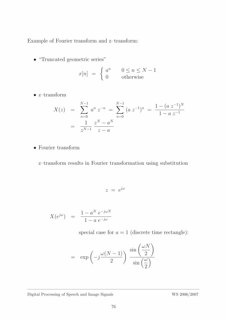
Example of Fourier transform and z–transform:
• “Truncated geometric series”
x[n] =
an 0 ≤ n ≤ N − 10 otherwise
• z–transform
X(z) =N−1∑
n=0
an z−n =N−1∑
n=0
(a z−1)n =1− (a z−1)N
1− a z−1
=1
zN−1
zN − aNz − a
• Fourier transform
z–transform results in Fourier transformation using substitution
z = ejω
X(ejω) =1− aN e−jωN
1− a e−jω
special case for a = 1 (discrete time rectangle):
= exp
(−jω(N − 1)
2
) sin
(ωN
2
)
sin(ω
2
)
Digital Processing of Speech and Image Signals WS 2006/2007
76

Proof for the z–transform inversion
• Statement:
x[k] =1
2πj
∮X(z) zk−1 dz
• Cauchy integration rule
1
2πj
∮z−kdz =
1 k = 10 k 6= 1
1
2πj
∮X(z) zk−1dz =
1
2πj
∮ ∑
n
x[n] z−n+k−1dz
=∑
n
x[n]1
2πj
∮z−n+k−1dz
︸ ︷︷ ︸6= 0 only for n = k
= x[k]
• Fourier:
z = ejω =⇒ dz = j ejω dω
Then:
x[n] =1
2πj
+π∫
−π
X(ejω) (ejω)n−1 j ejωdω
Integration path is unit circle because of ejω
=1
2π
+π∫
−π
X(ejω) ejωn dω
Digital Processing of Speech and Image Signals WS 2006/2007
77

2.8 System Representation and Examples
Example 1: Difference calculation
• Difference equation
y[n] = x[n] − x[n− n0], n0 integral number
• Fourier transform gives:∞∑
n=−∞y[n] e−jωn =
∞∑
n=−∞x[n] e−jωn −
∞∑
n=−∞x[n− n0] e
−jωn
Y (ejω) = X(ejω) −∞∑
n=−∞
(x[n] e−jωn e−jωn0
)
= X(ejω) − e−jωn0 X(ejω)
• Then follows:
H(ejω) =Y (ejω)
X(ejω)
= 1 − e−jωn0
|H(ejω)|2 = (1− cos(ωn0))2 + sin2(ωn0)
= 1 − 2cos(ωn0) + cos2(ωn0) + sin2(ωn0)
= 2 (1 − cos(ωn0))
|H(eiω)|2
0
1
2
3
4
5
ω πn0
Digital Processing of Speech and Image Signals WS 2006/2007
78

Example 2: First order difference equation
Delay
y[n]
x[n]
+
y[n-1]
α
x[n] + α y[n− 1] = y[n]
⇐⇒ y[n] − α y[n− 1] = x[n]
Method 1: Estimation of transfer function H(ejω)from impulse response h[n]:
• From the Eq. above with y[n] = h[n] and x[n] = δ[n] follows:
h[n] = δ[n] + α h[n− 1]
= δ[n] + α δ[n− 1] + α2 δ[n− 2] + · · ·
=
αn, n ≥ 00, otherwise
• Fourier spectrum/transfer function H(ejω)
H(ejω) =+∞∑
k=−∞h[k] e−jωk
=+∞∑
k=0
αk e−jωk
=+∞∑
k=0
(α e−jω
)k
=1
1 − α e−jωfor |α| < 1
Digital Processing of Speech and Image Signals WS 2006/2007
79

Method 2: Estimation of transfer function H(ejω) usingFourier transform of difference equation:
• Difference equation:
y[n] − α y[n− 1] = x[n]
• Fourier–transform:
Y (ejω) − α e−jω Y (ejω) = X(ejω)
• Result:
H(ejω) =Y (ejω)
X(ejω)
=1
1 − α e−jω
Digital Processing of Speech and Image Signals WS 2006/2007
80

Example 3: Linear difference equations (with constant coefficients)
• Difference equation:
y[n] =I∑
i=0
b[i] x[n− i]−J∑
j=1
a[j] y[n− j]
• z-transform:
Y (z) = X(z)I∑
i=0
b[i]z−i − Y (z)J∑
j=1
a[j]z−j
• Result:
H(z) =Y (z)
X(z)
=
I∑i=0
b[i] z−i
1 +J∑j=1
a[j] z−j
=+∞∑
n=−∞h[n] z−n
Using the definition of H(z) we can optain the impulse response as afunction of the coefficients of the difference equation in the above term.
Remark:
If we factorise denominator and numerator polynoms into linear fac-tors, we can obtain a zero-pole-representation of a discrete time LTIsystem:
H(i) =ΠIi=1(z − vi)
ΠJj=1(z − wj)
with zeros vi ∈ C and poles wj ∈ C.
Digital Processing of Speech and Image Signals WS 2006/2007
81

• in general:
h[n] has infinite number of non-zero values
=⇒ IIR–filter: Infinite Impulse Response
• but if: a[j] ≡ 0 ∀jh[n] identical to zero outside of a finite interval
h[n] =
b[n] n = 0, . . . , I0 otherwise
=⇒ FIR–filter: Finite Impulse Response
Digital Processing of Speech and Image Signals WS 2006/2007
82
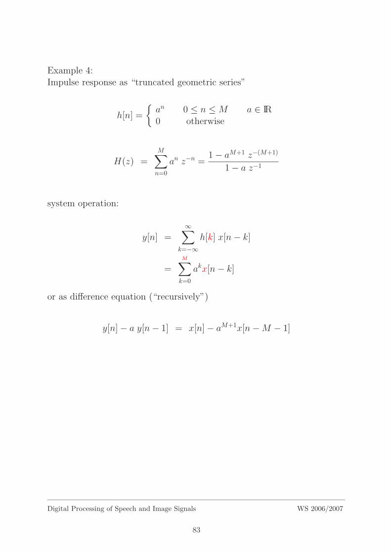
Example 4:Impulse response as “truncated geometric series”
h[n] =
an 0 ≤ n ≤M a ∈ IR0 otherwise
H(z) =M∑
n=0
an z−n =1− aM+1 z−(M+1)
1− a z−1
system operation:
y[n] =∞∑
k=−∞h[k] x[n− k]
=M∑
k=0
akx[n− k]
or as difference equation (“recursively”)
y[n]− a y[n− 1] = x[n]− aM+1x[n−M − 1]
Digital Processing of Speech and Image Signals WS 2006/2007
83

For this example we consider the zero-pole-representation:
H(z) =1− (za)
−(M+1)
1− (za)−1
α > 0
Zeros: zk = a · ej 2πkM+1 k = 0, 1, . . . ,M
Pole: z0 = a
(cancelled by zero z0 = a)
M=11
Re
Im
a
Digital Processing of Speech and Image Signals WS 2006/2007
84

Example 5:Fibonacci numbers
Difference equation:
n ≥ 0 h[n+ 2] = h[n+ 1] + h[n]
h[0] = h[1] = 1
n < 0 h[n] = 0
H(z) =∞∑
n=−∞h[n]z−n
= 1 + z−1 +∞∑
n=0
h[n+ 2]z−(n+2)
= 1 + z−1 +∞∑
n=0
h[n+ 1]z−(n+2) +∞∑
n=0
h[n]z−(n+2)
= 1 + z−1 + z−1∞∑
n=0
h[n+ 1]z−(n+1) + z−2∞∑
n=0
h[n]z−n
= 1 + z−1 (1 +∞∑
n=1
h[n]z−n)
︸ ︷︷ ︸H(z)
+ z−2∞∑
n=0
h[n]z−n
︸ ︷︷ ︸H(z)
= 1 + z−1H(z) + z−2H(z)
H(z)(1− z−1 − z−2) = 1
H(z) =1
1− z−1 − z−2
=1√5
( a
1− az−1− b
1− bz−1
)
where a =1 +√
5
2and b =
1−√
5
2
Digital Processing of Speech and Image Signals WS 2006/2007
85

For a and b the following holds:
1
1− (az )=
∞∑
n=0
( az
)n=
∞∑
n=0
anz−n
That results in:
H(z) =∞∑
n=0
1√5
(an+1 − bn+1
)z−n
!=
∞∑
n=0
h[n] z−n
h[n] =1√5
(an+1 − bn+1
)
Digital Processing of Speech and Image Signals WS 2006/2007
86

Table 2.1: Fourier transform pairs
signal Fourier–transform
1. δ[n] 1
2. δ[n− n0] e−jωn0
3. 1 (−∞ < n <∞)∞∑
k=−∞
2πδ(ω + 2πk)
4. anu[n] (|a| < 1)1
1− ae−jω
5. u[n]1
1− e−jω+
∞∑
k=−∞
πδ(ω + 2πk)
6. (n+ 1)anu[n] (|a| < 1)1
(1− ae−jω)2
7.rn sinωp(n+ 1)
sinωp
u[n] (|r| < 1)1
1− 2r cosωp e−jω + r2e−j2ω
8.sinωcn
πnX(ejω) =
1, |ω| < ωc,
0, ωc < |ω| ≤ π
9. x[n] =
1, 0 ≤ n ≤M
0, otherwise
sin[ω(M + 1)/2]
sin(ω/2)e−jωM/2
10. ejω0n
∞∑
k=−∞
2πδ(ω − ω0 + 2πk)
11. cos(ω0n+ φ) π
∞∑
k=−∞
[ejφδ(ω − ω0 + 2πk) + e−jφδ(ω − ω0 + 2πk)]
u[n] =
1, n ≥ 00, n < 0
Digital Processing of Speech and Image Signals WS 2006/2007
87

2.9 Discrete Time Signal Fourier Transform Theo-
rem
Basically there is no difference between FT theorem for the continuoustime and the discrete time case because summation has the same proper-ties as integration. Only differentiation and difference calculation are notcompletely analog, because it is not possible to form a derivative in thediscrete time case.
Table 2.2: Fourier transform Theorems
signal Fourier–transformx[n], y[n] X(ejω), Y (ejω)
1. ax[n] + by[n] aX(ejω) + bY (ejω)
2. x[n− nd], e−jωndX(ejω)nd is integral number
3. ejω0nx[n] X(ej(ω−ω0))
4. x[−n] X(e−jω)X(ejω) if x[n] is real
5. nx[n] jdX(ejω)
dω
6. x[n] ∗ y[n] X(ejω)Y (ejω)
7. x[n]y[n]1
2π
∫ π
−π
X(ejΘ)Y (ej(ω−Θ))dΘ
8. x[n]− x[n− 1] (1− e−jω)X(ejω)|1− e−jω|2 = 2(1− cosω)
Parseval theorem
9.∞∑
n=−∞
|x[n]|2 =1
2π
∫ π
−π
|X(ejω)|2dω
10.∞∑
n=−∞
x[n]y[n] =1
2π
∫ π
−π
X(ejω)Y (ejω)dω
Digital Processing of Speech and Image Signals WS 2006/2007
88

Example 1 corresponding to Theorem 5:
X(ejω) =+∞∑
k=−∞x[k] e−jωk
d
dωX(ejω) =
d
dω
(+∞∑
k=−∞x[k] e−jωk
)
=+∞∑
k=−∞
d
dω
(x[k] e−jωk
)
=+∞∑
k=−∞x[k] (−jk) e−jωk
⇐⇒ jd
dωX(ejω) =
+∞∑
k=−∞k x[k] e−jωk
F n · x[n] = jd
dωF x[n]
Example 2 corresponding to Theorem 8:
F x[n]− x[n− 1] =+∞∑
k=−∞x[k] e−jωk −
+∞∑
k=−∞x[k − 1] e−jωk
=+∞∑
k=−∞x[k] e−jωk −
+∞∑
k=−∞x[k] e−jωk e−jω
= X(ejω)(1− e−jω
)
=⇒ |F x[n]− x[n− 1] |2 = |F x[n] |2 |1 − e−jω|2= |F x[n] |2 2 · (1− cos(ω))
Digital Processing of Speech and Image Signals WS 2006/2007
89

2.10 Discrete Fourier Transform: DFT
The Fourier transform for discrete time signals and systems has been ex-plained on the previous pages. For discrete time signals with finite lengththere is also another Fourier representation called “Discrete Fourier Trans-form” (DFT).
The DFT plays a central role in digital signal processing.
Decisive reasons:
• fast algorithms exist for DFT calculation(Fast Fourier Transform, FFT).
• discrete frequencies ωk can be better represented in the computer thancontinuous frequencies ω.
Digital Processing of Speech and Image Signals WS 2006/2007
90

Assume a discrete time signal x[n] with finite length (see also chapter 3.2on page 135):
x[n] =
x[n] 0 ≤ n ≤ N − 10 otherwise
Note: For a continuous time signal it is impossible in the strict sense to beband-limited and time-limited (truncation effect = Windowing).
• The discrete time signal Fourier transform for x[n] is:
X(ejω) =N−1∑
n=0
x[n] exp(−jωn)
• ω is a continuous variable. The period is 2π. Frequency discretisationis made by sampling along the frequency axis.
• The Fourier transform X(ejω) is evaluated at
ωk =2π
Nk where k = 0, 1, . . . , N − 1
• Define:
X[k] : = X(ejω)|ω = ωk
N=8
Re
ImC
Digital Processing of Speech and Image Signals WS 2006/2007
91

• Discrete Fourier Transform (DFT):
X[k] =N−1∑
n=0
x[n] exp(−j 2π
Nk n), k = 0, 1, . . . , N − 1
• Inverse DFT:
x[n] =1
N
N−1∑
k=0
X[k] exp(j2π
Nk n), n = 0, 1, . . . , N − 1
• Remark:
This equation can be proven by inserting the equation for X[k] in theequation for x[n] and using the orthogonality:
1
N
N−1∑
n=0
exp
(j2π
Nkn
)=
1 k = m N, m is integral number0 otherwise
• Note:
Consider the “analogy” between inverse DFT (above) and inverseFourier transform of discrete time signal:
x[n] =1
2π
2π∫
0
X(ejω) ejωn dω
Under the given conditions the integral is equal to the sum(without approximation!).
Digital Processing of Speech and Image Signals WS 2006/2007
92

Remarks:
• DFT coefficients X[k] are not an approximation of the discrete timesignal Fourier transform X(ejω). On the contrary:
X[k] = X(ejω)|ω = ωk
• Number of the coefficients X[k] depends on the signal length N . Afiner sampling of the discrete time signal Fourier transform is possibleby appending zeros to the signal x[n] (Zero–Padding).
x[n]
nN-1
Digital Processing of Speech and Image Signals WS 2006/2007
93

Interpretation of Fourier coefficients
• Fourier transform X(ejω) of the time discrete signal x[n]
|X(e )|
ωπ−π
ωj
• Evaluation at N discrete sampling points
ωk =2π
Nk
yields the DFT coefficients X[k].
At first k lies in the domain k = −N2
+ 1, . . . , 0, . . . ,N
2.
|X(e )|, |X[k]|
ωπ−π
ωj
-N/2+1 N/21 20-1 k
Digital Processing of Speech and Image Signals WS 2006/2007
94

• Because of the periodicity of X(ejω) the coefficients X[k] can also beobtained by shifting the sampling points with negative frequency intothe positive frequency domain (by one period).
Then k = 0, . . . , N/2, . . . , N − 1.
X[k] =N−1∑
n=0
x[n] exp(−j 2π
Nk n)
|X(e )|, |X[k]|
ωπ−π
ωj
1 20 N-1 k
• Interpretation of coefficients for general signal x[n]:
k = 0 ←→ f = 0
1 ≤ k ≤ N
2− 1 ←→ 0 < f <
fS2
k =N
2←→ ±fS
2N
2+ 1 ≤ k ≤ N − 1 ←→ −fS
2< f < 0
Digital Processing of Speech and Image Signals WS 2006/2007
95

Symmetric relations by real signals:
• For DFT coefficients X[k] of a real signal x[n] the following holds:
X[k] = X[N − k]
Re(X[k]) = Re(X[N − k])Im(X[k]) = −Im(X[N − k])
• For the amplitude spectrum |X[k] | the following holds:
|X[k] |2 = Re2X[k] + Im2X[k]= |X[N − k] |2
Digital Processing of Speech and Image Signals WS 2006/2007
96

Realization of DFT:
/* PI = 3.14159265358979 */
/* x: input signal */
/* N: length of input signal */
/* Xre, Xim: real and imaginary part of DFT coefficients */
void dft (int N, float x[], float Xre[], float Xim[])
int n, k;
float SumRe, SumIm;
for (k=0; k<=N-1; k++)
SumRe = 0.0;
SumIm = 0.0;
for (n=0; n<=N-1; n++)
SumRe += x[n]*cos(2*PI*k*n/N);
SumIm -= x[n]*sin(2*PI*k*n/N);
Xre[k] = SumRe;
Xim[k] = SumIm;
Remark:
• discrete realization
• Reduction of “Fourier powers” e−2πjN·kn to e−
2πjN·l (l = 0, 1, . . . , N − 1)
is possible, because they are periodical (on the unit circle).
Digital Processing of Speech and Image Signals WS 2006/2007
97

2.11 DFT as Matrix Operation
• Notation with unit roots
X[k] =N−1∑
n=0
x[n] exp (−2πj
Nk n)
=N−1∑
n=0
x[n] W knN
where WN := exp (−2πj
N)
N=12
W =10N
W 1N
W 2NW 3N
• Periodicity of WN
unit root:
exp (−j ωk) = exp (−j2πNk) = (WN)k
WN := exp (−j2πN
)
Digital Processing of Speech and Image Signals WS 2006/2007
98

Note:
1. W rN = W r mod N
N
2. W kNN = (WN
N )k = 1k = 1 k ∈ Z
3. W 2N = [exp (−2πj
N)]2 = exp (−2πj
N2)
= exp (− 2πj
N/2) = WN/2 N even
4. WN/2N = exp (−2πj
N
N
2) = exp (−πj) = −1
5. Wr+N/2N = W
N/2N W r
N = −W rN
Digital Processing of Speech and Image Signals WS 2006/2007
99

DFT as matrix multiplication
X[k] =N−1∑
n=0
x[n] exp (−2πj
Nk n)
=N−1∑
n=0
W knN x[n]
=N−1∑
n=0
WNkn x[n]
with the matrix WN and the matrix elements:
WNkn := W knN
Inversion:
x[n] =1
N
N−1∑
k=0
X[k] exp (2πj
Nk n)
=1
N
N−1∑
k=0
(W−1N )kn X[k]
=1
N
N−1∑
k=0
W−1N kn X[k]
Therefore for the matrix WN−1 holds:
WN−1 :=1
NW−1
N
Digital Processing of Speech and Image Signals WS 2006/2007
100

DFT matrix operation: properties
• DFT: invertible linear mapping
N complex signal values ↔ N complex Fourier components
N real signal values ↔ N
2complex Fourier components
(due to symmetry)
in words:DFT causes no “information loss” in the signal.
• Parseval theorem for DFTgeneral Fourier:
N−1∑
n=0
|x[n]|2 =1
2π
+π∫
−π
|X(ejω)|2dω
special DFT: (recalculate for yourself!)
N−1∑
n=0
|x[n]|2 =1
N
N−1∑
k=0
|X[k]|2
in words:
Disregarding the factor1
N, the DFT is a norm conserving (= energy
conserving) transformation (mathematical terminology: “unitary”).
Digital Processing of Speech and Image Signals WS 2006/2007
101

2.12 From Continuous Fourier Transform to Matrix
Representation of Discrete Fourier Transform
Assumption: band-limited signal x(t)
Fourier transform of the continuous time signal x(t):
X(ω) = Fx(t) =
∫ ∞
−∞x(t) e−jωtdt (2.9)
For the exact reconstruction (without approximation) of the continuoustime signal from sampled values, the samples x[n] = x(n · Ts) must havethe distance of at most
Ts =π
ωB
(sampling theorem).
This results in the Fourier transform of the discrete time signal x[n]:
X(ejω) =∞∑
−∞x[n] e−jωn (2.10)
where ω is frequency “normalised on T ′′s
Functions (2.9) and (2.10) agree in interval [−ΩS/2,+ΩS/2] = [−ωB,+ωB].
X
ω
(ω)||
−ω ωBB
ΩS−ΩS
Digital Processing of Speech and Image Signals WS 2006/2007
102

0
0.2
0.4
0.6
0.8
1
0 N-10
0.2
0.4
0.6
0.8
1
0 N-1
Figure 2.12: Hanning window
The signal x[n] is further decomposed by applying a window function w[n](windowing):
w[n] =
. . . n = 0, . . . , N − 1
0 otherwise
Windowed signal y[n]:y[n] = w[n] · x[n]
can be analyzed using Fourier transform or DFT.
Y (ejωk) =N−1∑
n=0
y[n] e−jωk
DFT:
ωk =2πk
Nwhere k = 0, . . . , N − 1
Y [k] =N−1∑
n=0
y[n] e−2πNkn
Matrix representation:
K = N
Y [0]...
Y [k]...
Y [K − 1]
=
...
e−2πjN·n·k
...
y[0]...
y[n]...
y[N − 1]
Digital Processing of Speech and Image Signals WS 2006/2007
103

2.13 Frequency Resolution and Zero Padding
Task: signal x[n] with finite length N is given.
Wanted: Fourier transform X(ejωk) at
ωk =2π
Kk, where k = 0, 1, . . . , K − 1 and K > N
Inserting the definitions:
X(ejωk) =N−1∑
n=0
x[n] exp (−2πj
Kk n)
=K−1∑
n=0
x[n] exp (−2πj
Kk n)
where x[n] =
x[n] n = 0, . . . , N − 10 n = N, . . . ,K − 1
i.e. Zero Padding (appending zeros).
Matrix representation:
X[0]...
...X[K − 1]
=
W nkK
x[0]...
...x[N − 1]
0...0
n = 0
n = N − 1n = N
n = K − 1
Note:“Zero Padding” does not introduce any additional information into the sig-nal. This is only a trick so that DFT and particularly FFT (Fast FourierTransform) can be performed with a
higher frequency resolution .
Digital Processing of Speech and Image Signals WS 2006/2007
104

2.14 Finite Convolution
Input signal and convolution kernel have finite duration
Consider “finite” convolution:
• Impulse response: h[n] ≡ 0 for n 6∈ 0, 1, 2, . . . , Nh − 1
• Input signal: x[n] ≡ 0 for n 6∈ 0, 1, 2, . . . , Nx − 1
• Output signal:
y[n] =∞∑
k=−∞h[k] x[n− k]
=
Nh−1∑
k=0
h[k] x[n− k]
k
k
h[k]
x[-k]
N-1
-(N-1)x
h
0
n=0
• Altogether: Nx +Nh − 1 positions with “overlap”
• Therefore only Nx + Nh − 1 values of output signal can be differentfrom zero:
y[n] =
0 n > Nx +Nh − 2. . . n = 0, 1, . . . , Nx +Nh − 20 n < 0
Digital Processing of Speech and Image Signals WS 2006/2007
105

k0 Nh-1=12
1
k0 Nx-1=4
x[k]
1 0.80.6
0.40.2
k0-Nx
x[n-k] n=-1,
k0
x[n-k] n=m (m>0 & m<Nh+Nx-2),
k0
x[n-k] n=Nh+Nx-1,
n0
y[n]
-1 Nh-1
Nh-1
Nh+Nx-1
mm-NX+1
Nh+Nx-2
Nh-1
a)
b)
c)
i)
ii)
iii)
Nh-1
1
1.8
2.4
2.8
2
1.2
0.60.2
3 3
Nx-1
h[k]
Figure 2.13: Example of a linear convolution of two finite length signals: a) two signals;b) signal x[n-k] for different values of n:i) n < 0, no overlap with h[k], therefore convolution y[n] = 0ii) n between 0 and Nh +Nx − 2, convolution 6= 0iii) n > Nh +Nx − 2, no overlap with h[k], convolution y[n] = 0c) resulting convolution y[n].
Digital Processing of Speech and Image Signals WS 2006/2007
106

Finite convolution using DFT
Convolution theorem:
y[n] =∞∑
k=−∞h[k] x[n− k]
Fourier:
Y (ejω) = H(ejω) X(ejω), 0 ≤ ω ≤ 2π
Also valid for sample frequencies:
ωk :=2π
Nk, k = 0, . . . , N − 1 for any N
Notation: Y [k] = H[k] X[k]
• Question: How to choose the length N of the DFT ?
– Reminder: different “lengths”
– x[n]: Nx non-zero values
– h[n]: Nh non-zero values
– y[n]: Ny = Nx +Nh − 1 non-zero values
• Answer:
– The convolution theorem is certainly correct for any N > 0.
– If we want to calculate the output signal completely from Y [k],we have to know Y [k] for
at least N = Nx +Nh − 1frequency values k = 0, 1, . . . , N − 1.
– In words: for the DFT length N must be valid:
N ≥ Nx + Nh − 1
Method: Zero Padding, i.e. appending zeros.
Note: The FFT will be introduced on the next pages. A comparison ofcosts for realization of the finite convolution by DFT and FFT can befound at the end of paragraph 2.15.
Digital Processing of Speech and Image Signals WS 2006/2007
107

2.15 Fast Fourier Transform (FFT)
Principle of FFT:Calculation of the DFT can be done by successive decomposition intosmaller DFT calculations. In this way, the number of elementary oper-ations (multiplications and additions) is dramatically reduced:
FFT:
N 2 → N
2ldN operations
N = 1024 :2 ·NldN
=2 · 1024
10= 200 factor of velocity gain
The matrix is decomposed into a product of sparse matrices, therefore Nwith lot of prime factors is convenient (not necessarily only powers of two).
Terminology for different variants of FFT:
• in time ↔ in frequency
• in place: yes/no
• radix 2 ↔ radix 4
• decomposition to prime factors instead of N = 2n
History
1965 Cooley and Tukey1942 Danielson and Lanczos1905 Runge1805 Gauss
Digital Processing of Speech and Image Signals WS 2006/2007
108

Algorithms which are based on a decomposition of the signal x[n] are called“decimation–in–time algorithms”.
The case N = 2ν is considered in the following.
X[k] =N−1∑
n=0
x[n] exp(−j 2π
Nk n) where k = 0, 1, . . . , N − 1
=N−1∑
n=0
x[n] W nkN where W nk
N = exp(−j 2π
Nk n)
• Decomposition of the sum over n into the sums over even and odd n:
X[k] =
N/2−1∑
r=0
x[2r] W 2rkN +
N/2−1∑
r=0
x[2r + 1] W(2r+1)kN
=
N/2−1∑
r=0
x[2r] (W 2N)rk + W k
N
N/2−1∑
r=0
x[2r + 1] (W 2N)rk
• Because of
W 2N = exp(−2j
2π
N) = exp(−j 2π
N/2) = WN/2
for k = 0, . . . , N − 1 holds:
X[k] =
N/2−1∑
r=0
x[2r] W rkN/2 + W k
N
N/2−1∑
r=0
x[2r + 1] (WN/2)rk
= G[k] + W kN H[k]
• Each of the two sums corresponds to the DFT with the length N/2.The first sum is a N/2–DFT of the even indexed signal values x[n],the second sum is a N/2–DFT of the odd indexed values.
• The DFT of the length N can be obtained by getting the two N/2–DFT’s together, with the factor W k
N .
Digital Processing of Speech and Image Signals WS 2006/2007
109

Complexity:The complexity O(N 2) of one-dimensional FT can be reduced by adequateresorting values from two FTs with length N
2 and complexity O(2 · (N2 )2) =N2
2 . By successive application of this resorting the complexity can be re-duced to O(N logN).The case N = 23 = 8 is considered in the following.
• X[4] can be obtained from H[4] and G[4] according to previous equa-tion.
• Because of the DFT–length N2 = 4:
H[4] = H[0] and G[4] = G[0]
And then:
X[4] = G[0] + W 4N H[0]
The values X[5], X[6] and X[7] can be obtained analogously.
Flow diagram for decomposition of one N -DFT into two N/2–DFTs:
x[n] X[k]
N/2-point
DFT
N/2-point
DFT
x[0]
x[2]
x[4]
x[6]
x[1]
x[3]
x[5]
x[7]
G[0]
G[1]
G[2]
G[3]
H[0]
H[1]
H[2]
H[3]
X[0]
X[1]
X[2]
X[3]
X[4]
X[5]
X[6]
X[7]
W0N
W1N
W2N
W3N
W4N
W5N
W6N
W7N
Figure 2.14: Flow diagram for decomposition of one N -DFT to two N/2–DFTs withN = 8
Digital Processing of Speech and Image Signals WS 2006/2007
110

• Further analogous decomposition, until only DFT’s with the lengthN = 2 remain (so called Butterfly Operation)
• Resulting flow diagram of the FFT:
x[n] X[k]x[0]
x[4]
x[2]
x[6]
x[1]
x[5]
x[3]
x[7]
W0N
W0N
W0N
W0N
-1
-1
-1
-1
W0N
W2N
-1
-1
-1
-1
W0N
W1N
W2N
W3N
X[0]
X[1]
X[2]
X[3]
X[4]
X[5]
X[6]
X[7]
W0N
W2N
-1
-1
-1
-1
Figure 2.15: Flow diagram of an 8–point–FFT using Butterfly operations.
Digital Processing of Speech and Image Signals WS 2006/2007
111

Complexity reduction
• Number of complex multiplications in FFTis N/2 · ldN .
• Comparison:Direct application of the DFT definition needsN 2 complex multiplications.
• Example: N = 1024 = 210
N 2
N/2 · ldN≈ 200
Complexity reduction by factor 200
FFT with the base 2 is not minimal according to number of addi-tions, FFT with the base 4 can be better.
Digital Processing of Speech and Image Signals WS 2006/2007
112

Matrix representation of the FFT principle
• The complex Fourier matrix can be decomposed into the product ofr = ldN matrices, each of them having only two non-zero elements ineach column.
• The following graph shows the decomposition of the Fourier matrix inthe case of inverse transformation.
• w corresponds to W−1N
X = |wnk|X = T3 · T2 · T1 · TS · x
This is how the decomposition into r + 1 = 4 matrices looks like(w4 = −1, w8 = 1):
1 1 1 1 1 1 1 1 1 1 1 1 1 1 1 11 w w2 w3 w4 w5 w6 w7 1 w w2 w3 w4 w5 w6 w7
1 w2 w4 w6 w8 w10 w12 w14 1 w2 w4 w6 1 w2 w4 w6
1 w3 w6 w9 w12 w15 w18 w21 1 w3 w6 w w4 w7 w2 w5
|wnk| = 1 w4 w8 w12 w16 w20 w24 w28 = 1 w4 1 w4 1 w4 1 w4
1 w5 w10 w15 w20 w25 w30 w35 1 w5 w2 w7 w4 w w6 w3
1 w6 w12 w18 w24 w30 w36 w42 1 w6 w4 w2 1 w6 w4 w2
1 w7 w14 w21 w28 w35 w42 w49 1 w7 w6 w5 w4 w3 w2 w
Digital Processing of Speech and Image Signals WS 2006/2007
113

Signal flow diagram
The calculation operations which correspond to the matrix representationof FFT can be showed in a signal flow diagram.
T3 T2 T1 TS1 0 0 0 1 0 0 0 1 0 1 0 0 0 0 0 1 1 0 0 0 0 0 0 1 0 0 0 0 0 0 00 1 0 0 0 w 0 0 0 1 0 w2 0 0 0 0 1 -1 0 0 0 0 0 0 0 0 0 0 1 0 0 00 0 1 0 0 0 w2 0 1 0 -1 0 0 0 0 0 0 0 1 1 0 0 0 0 0 0 1 0 0 0 0 00 0 0 1 0 0 0 w3 0 1 0 −w2 0 0 0 0 0 0 1 -1 0 0 0 0 0 0 0 0 0 0 1 0
1 0 0 0 −1 0 0 0 0 0 0 0 1 0 1 0 0 0 0 0 1 1 0 0 0 1 0 0 0 0 0 00 1 0 0 0 −w 0 0 0 0 0 0 0 1 0 w2 0 0 0 0 1 -1 0 0 0 0 0 0 0 1 0 00 0 1 0 0 0 −w2 0 0 0 0 0 1 0−1 0 0 0 0 0 0 0 1 1 0 0 0 1 0 0 0 00 0 0 1 0 0 0 −w3 0 0 0 0 0 1 0 −w2 0 0 0 0 0 0 1 -1 0 0 0 0 0 0 0 1
TS T1 T2 T3
-1
-1
-1
-1
-1
-1
-1
ω2
ω2
-1
ω
ω2
ω3
−1
−1
−1
−1
X[0]
X[1]
X[2]
X[3]
X[4]
X[5]
X[6]
X[7]
x[0]
x[1]
x[2]
x[3]
x[4]
x[5]
x[6]
x[7]
Digital Processing of Speech and Image Signals WS 2006/2007
114

• Matrices T1, T2 and T3 contain exactly two non-zero elements in eachrow.
• Non-zero elements are realizing the Butterfly Operation.
• Matrix T1: step width of the Butterfly Operation is 1Matrix T2: step width of the Butterfly Operation is 2Matrix T3: step width of the Butterfly Operation is 4
• step widths can be found:
– in signal flow diagram
– distance between the non-zero elements in T1, T2 and T3
Digital Processing of Speech and Image Signals WS 2006/2007
115

Butterfly Operation
• Signal flow diagram and matrix representation of the FFT are basedon the following basic operation:
Xm-1[p]
Xm-1[q]
Xm[p]
Xm[q]-1
WrN
• For two input values Xm−1[p] and Xm−1[q] this operation producestwo output values Xm[p] and Xm[q]. The output values are thereby alinear combination of the input values.
• Because of the flow graph, the operation is called“Butterfly Operation”.
Xm[p] = Xm−1[p] +W rN Xm−1[q]
Xm[q] = Xm−1[p]−W rN Xm−1[q]
[Xm[p]Xm[q]
]=
[1 W r
N
1 −W rN
] [Xm−1[p]Xm−1[q]
]
Digital Processing of Speech and Image Signals WS 2006/2007
116

Bit Reversal
• The matrix representation of the FFT uses a sorting matrix, i.e. thesignal which is to be transformed is at first resorted.
• Example for N = 8:
n Binary representation Reversed n’
0 000 000 01 001 100 42 010 010 23 011 110 64 100 001 15 101 101 56 110 011 37 111 111 7
• Bit Reversal is a necessary part of the FFT–Algorithm.
Bit Reversal for N = 23
Digital Processing of Speech and Image Signals WS 2006/2007
117

2.16 FFT Implementation
• Fortran version
C adapted from: Oppenheim, Schafer p. 608
C SUBROUTINE FFT DecimationInTime (X, ld n) **********************************
C ****************************************************************************
PARAMETER PI = 3.14159265358979
PARAMETER N max = 2048
COMPLEX X(N max) ! array for input AND output
COMPLEX Temp ! temporary storage
COMPLEX W uni ! root of unity
COMPLEX W pow ! powers of W uni
INTEGER N, ld N, ip, iq, iqbeq, j, k, i exp, istp
N = 2**ld n
IF (N.GT.N max) STOP
C BIT Reversed Sorting *********************************************************
j = 1
DO i = 1, N-1
IF (i.LT.j) THEN ! swap X(j) and X(i)
Temp = X(j)
X(j) = X(i)
X(i) = Temp
ENDIF
k = N/2
DO WHILE (k.LT.j)
j = j - k
k = k / 2
ENDDO
j = j + k
ENDDO
C End of Bit Reversed Sorting **************************************************
C FFT Butterfly Operations *****************************************************
DO i=1, ld N
i exp = 2**i ! exponent
istp = i exp/2 ! stepsize
W pow = (1.0,0.0)
W uni = CMPLX (COS (PI/FLOAT(istp)), -SIN(PI/FLOAT(istp)))
DO ipbeg = 1, istp
DO ip = ipbeg, N, i exp
iq = ip + istp
Temp = X(iq) * W pow
X(iq) = X(iq) - Temp
X(ip) = X(iq) + Temp
ENDDO
W pow = W pow * W uni
ENDDO
ENDDO
C End of FFT Butterfly Operations **********************************************
RETURN
END
Digital Processing of Speech and Image Signals WS 2006/2007
118

Explanations about Fortran Program
Two program parts:
1. Bit Reversal
2. Butterfly Operations
• 3 loops with variables i, ipbeg, ip are controlling the execution ofthe Butterfly operations
• outer loop i:i specifies the level of the FFT
• With exception of the first level, Butterfly operations are “nested”.Therefore two loops are used for the Butterfly operations withinone level.
• middle loop, ipbeg:ipbeg: goes over the “nested” Butterfly operationsi=1: ipbeg=1i=2: ipbeg=1,2i=3: ipbeg=1,2,3,4iqbeg: specifies the sequence of starting points for inner loop
• inner loop, ip:ip: specifies the first element of the Butterfly operationistp: step width of the Butterfly operationiq=ip+istp: specifies the second element for Butterfly operationinner loop is “started” once per “nesting”
Digital Processing of Speech and Image Signals WS 2006/2007
119

x[0]
x[4]
x[2]
x[6]
x[1]
x[5]
x[3]
x[7]
W0N
W0N
W0N
W0N
-1
-1
-1
-1
W0N
W2N
-1
-1
-1
-1
W0N
W1N
W2N
W3N
X[0]
X[1]
X[2]
X[3]
X[4]
X[5]
X[6]
X[7]
W0N
W2N
-1
-1
-1
-1
Figure 2.16: Flow diagram of an 8–point–FFT using Butterfly operations.
Digital Processing of Speech and Image Signals WS 2006/2007
120

• C version (from Numerical Recipes in C)
#include <math.h>#define SWAP(a,b) tempr=(a);(a)=(b);(b)=tempr
void four(float data[], unsigned long nn, int isign)
Replaces data[1..2*nn] by its discrete Fourier transform, if isign is input as 1; or replacesdata[1..2*nn] by nn times its inverse discrete Fourier transform if insign is input as -1.data is a complex array of lenght nn or, equivalently, a real array of lenght 2*nn. nn MUSTbe an whole number power of 2 (this is not checked for!).
unsigned long n, mmax, m, j, istep, i;
double wtemp, wr, wpr, wpi, wi, theta; Double prec. for the trigonometric recurrences.float tempr, tempi;
n=nn << 1;
j=1;
for (i=1; i<n; i+=2) This is the bit-reversal section of the routine.if (j > i)
SWAP (data[j], data[i]); Exchange the two complex numbers.SWAP (data[j+1], data[i+1]);
m=n >> 1;
while (m >= 2 && j > m) j -= m;
m >>= 1;
j += m;
Here begins the Danielson-Lanczos section of the routine.mmax=2;
while (n > mmax) Outer loop executed log2 nn timesistep=mmax << 1;
theta=isign∗(6.28318530717959/mmax); Initialise the trigonometric recurrence.wtemp=sin(0.5*theta):
wpr = -2.0*wtemp*wtemp;
wpi=sin(theta);
wr=1.0;
wi=0.0;
for (m=1;m <mmax;m+=2) Here are the two nested loops.for (i=m;i<=n;i+=istep)
j=i+mmax; This is the Danielson-Lanczos formula:tempr=wr*data[j]-wi*data[j+1];
tempi=wr*data[j+1]+wi*data[j];
data[j]=data[i]-tempr;
data[j+1]=data[i+1]-tempi;
data[i] += tempr;
data[i+1] += tempi;
wr=(wtemp=wr)*wpr-wi*wpi+wr; Trigonometric recurrencewi=wi*wpr+wtemp*wpi+wi;
mmax=istep
Digital Processing of Speech and Image Signals WS 2006/2007
121

• Input and output arrays (C version)
1 real
2 imag
3 real
4 imag
2N-3
2N-2
2N-1
2N
real
imag
real
imag
a)
t = 0
t = ∆
t = (N-2)∆
t = (N-1)∆
1 real
imag
3 real
4 imag
b)
f = 0
f =
2
1N∆
2N-1
2N
real
imagf = 1
N∆
N+3
N+4
real
imag
N+1
N+2
real
imag
N-1
N
real
imagf = N/2 - 1
N∆
f = N/2 - 1N∆
f = 12∆
Figure 2.17: Input and output arrays of an FFT. a) The input array contains N (N ispower of 2) complex input values in one real array of the length 2N . with alternatingreal and imaginary parts. b) The output array contains complex Fourier spectrum at Nfrequency values. Again alternating real and imaginary parts. The array begins with thezero-frequency and then goes up to the highest frequency followed with values for thenegative frequencies.
Digital Processing of Speech and Image Signals WS 2006/2007
122

Finite convolution: complexity by the application of FFT
Estimation of number of necessary multiplications for a convolution of x[n]and h[n]
x[n]: Nx non-zero values
h[n]: Nh non-zero values
Realisation
direct implementation DFT FFT
transformation
(Nx +Nh)2 Nx+Nh
2 log2(Nx +Nh)
Nx ·Nh multiplication in frequency domain
Nx +Nh Nx +Nh
inverse transformation
(Nx +Nh)2 Nx+Nh
2 log2(Nx +Nh)
Digital Processing of Speech and Image Signals WS 2006/2007
123

2.17 Cyclic Matrices and Fourier Transform
The Fourier transform plays a significant role for so-called cyclic matrices(cf. chapter 3.8):
0 n N − 1
H =
h0 h1 h2 . . . hN−1
hN−1. . . . . . . . . hN−2
hN−2. . . . . . . . . . . . ...
. . . . . . . . . . . .... . . . . . . . . . h2
. . . . . . h1
h1 hN−1 h0
0
m
N − 1
so: Hmn = h(n−m)modN
with so-called kernel vector (h0, h1 . . . , hN−1)T and hn ∈ C, mostly hn ∈ IR.
Remark: using cyclic matrices it is possible to define cyclic i.e. periodicconvolutions and to build a cyclic variant of the system theory.
The eigenvectors of a cyclic matrix can be obtained from the columns ofDFT matrix:
0 n N − 1
0
m
N − 1
w0·0 · · · wn·0 · · · w(N−1)·0... wn·1 ......
...
· · · ... · · · ......
...
· · · ... · · · ...... wn·(N−1) ...
where w = e−2πjN
Digital Processing of Speech and Image Signals WS 2006/2007
124

The eigenvalues λk of a cyclic matrix with the kernel vector (h0, h1 . . . , hN−1)T
are:
λk =N−1∑
n=0
hn e− 2πj
N·k·n where k = 0, 1 . . . , N − 1
The representation is oriented on L. Berg: Linear equation systems withband structure (page 52 ff).
The special case of a cyclic matrix when the kernel vector h is symmetricand real is especially interesting for many applications:
hn = hN−n and hn ∈ IR
That means that the matrix is real, symmetric and cyclic:
0 N − 1
0
N − 1
h0 h1 h2 . . . h2 h1
h1. . . . . . . . . h2. . . . . . . . . . . . h3
. . . . . . . . . . . . ...... . . . . . . . . .
h2 h3. . . . . . h1
h1 h2 h1 h0
Digital Processing of Speech and Image Signals WS 2006/2007
125

For such a matrix is valid:
a) the eigenvalues λk are:
λk =N−1∑
n=0
hn cos( 2πkn
N
)
b) The eigenvectors can be obtained from the columns of the “discretecos–matrix”:
n
m
...
...
...cos
(2πnmN )
...
...
...
Application: diagonalisation of covariance matrices, e.g. for codingof image and speech signals.
Digital Processing of Speech and Image Signals WS 2006/2007
126

Proof:
We will prove that
vk =
cos 2πk·0N
cos 2πk·1N
...
...
...
cos 2πk·(N−1)N
are eigenvectors of the given matrix with eigenvalues λk.
For a symmetric cyclic matrix is valid:
Hmn := h(n−m)modN where hn = hN−n
One row results in (for odd N):
∑
n
Hmn · vkn = h0 · cos2πkm
N+
N−1
2∑
l=1
hl·(
cos2πk(m− l)
N+ cos
2πk(m+ l)
N
)
For even N only one term for l = (N − 1)/2 can go into the sum.
According to addition theorem:
cos(x+ y) + cos(x− y) = 2 · cosx · cos y
With x = 2πkm/N and y = 2πkl/N follows:
∑
n
Hmn · vkn = h0 · cos2πkm
N+ 2
N−1
2∑
l=1
hl·(
cos2πkl
N· cos
2πkm
N
)
=[h0 + 2
N−1
2∑
l=1
hl cos2πkl
N
]
︸ ︷︷ ︸λk
· cos2πkm
N︸ ︷︷ ︸vkm
= λk · vkm
Digital Processing of Speech and Image Signals WS 2006/2007
127

Excursion: Toeplitz matrices
We consider only quadratic real matrices:
H ∈ IRN×N with Hmn ∈ IR
a) H is a (general) Toeplitz matrix , if:
Hmn = hn−m
i.e.
H =
h0 h1 h2 . . . hN−2 hN−1
h−1. . . . . . . . . hN−2
h−2. . . . . . . . . . . . ...
... . . . . . . . . . . . . . . .
. . . . . . . . . . . . h2
h2−N. . . . . . . . . h1
h1−N h2−N h−2 h−1 h0
b) For a symmetric Toeplitz matrix then holds:
Hmn = h|n−m|
i.e.
H =
h0 h1 h2 . . . hN−2 hN−1
h1. . . . . . . . . hN−2
h2. . . . . . . . . . . . ...
... . . . . . . . . . . . . . . .
. . . . . . . . . . . . h2
hN−2. . . . . . . . . h1
hN−1 hN−2 h2 h1 h0
Digital Processing of Speech and Image Signals WS 2006/2007
128

c) A cyclic matrix can be obtained by special choice:
Hmn = h(n−m)modN
H =
h0 h1 h2 . . . hN−2 hN−1
hN−1. . . . . . . . . hN−2
hN−2. . . . . . . . . . . . ...
. . . . . . . . . . . .
... . . . . . . . . . h2
h2. . . . . . h1
h1 h2 hN−1 h0
Also valid: each cyclic matrix is a Toeplitz matrix.
d) A symmetric cyclic matrix can be obtained by the following choice ofthe kernel vectors h:
hn = hN−n for n = 0, . . . , N
For example, we obtain for N = 8:
H =
h0 h1 h2 h3 h4 h3 h2 h1
h1 h0 h1 h2 h3 h4 h3 h2
h2 h1 h0 h1 h2 h3 h4 h3
h3 h2 h1 h0 h1 h2 h3 h4
h4 h3 h2 h1 h0 h1 h2 h3
h3 h4 h3 h2 h1 h0 h1 h2
h2 h3 h4 h3 h2 h1 h0 h1
h1 h2 h3 h4 h3 h2 h1 h0
Digital Processing of Speech and Image Signals WS 2006/2007
129


Chapter 3
Spectral analysis
• Overview:
3.1 Features for Speech Recognition
3.2 Short Time Analysis and Windowing
3.3 Autocorrelation function and Power Spectral Density
3.4 Spectrograms
3.5 Filter Bank Analysis
3.6 Mel–Scale
3.7 Cepstrum
- Cepstrum Calculation from Filter Bank Output
- Mel–Cepstrum according to Davis and Mermelstein
3.8 Statistical Interpretation of Cepstrum Transformation
3.9 Energy in acoustic Vector
Digital Processing of Speech and Image Signals WS 2006/2007
131

3.1 Features for Speech Recognition
Architecture of an automatic speech recognition system
speech signal
short-timeanalysis
each 10 ms(using FFT)
sequence ofacoustic vectors
patterncomparison
decision
reference modelfor each word
in the vocabulary
Digital Processing of Speech and Image Signals WS 2006/2007
132

Short time analysis:
• window length 10–40ms
• sampling period 10–20ms
• in case of sampling rate of 10kHz:
– Window: 100–400 samples
– sampling period (frame shift): 100–200 samples
Recommended windows:
• Hamming
• Kaiser
• Blackman
Model parameters:
• Energy, intensity (“loudness”)
• Fundamental frequency (“height”)
• Spectral parameters (“colour”, “smoother” amplitude spectrum)
Digital Processing of Speech and Image Signals WS 2006/2007
133

Goal:
• Ideally: Real features for the recognition
• In practice: Data reduction, i.e. compact descriptionof the speech signal (amplitude spectrum)
Side effect:
• Method also enables coding of speech signals using lowest possiblenumber of bits
Key words:
• Fourier transform: wide band/narrow band, autocorrelation function
• Filter bank
• Cepstrum
• Linear Predictive Coding (LPC) analysis
• Fundamental frequency analysis
Digital Processing of Speech and Image Signals WS 2006/2007
134

3.2 Short Time Analysis and Windowing
• The DFT is defined for signals with finite duration.
• Speech signal s[n]:quasi stationary, i.e. properties do not change within 20-50 ms.
• Window function w[n]:Decomposition of the original signal s[n] into (overlapping)segments using a window function w[n]:
x[n] = s[n] · w[n]
where for example
w[n] =
1, |n| ≤ N/20, otherwise
• The windowed signal x[n] is analyzed with a Fourier Transform orDFT.
• The multiplication of the original signal s[n] with the window functionw[n] in the time domain corresponds to the convolution of the spectraof two signals S(ejω) and window function W (ejω) in the frequencydomain:
X(ejω) =1
2π
π∫
−π
S(ejθ) W (ej(ω−θ)) dθ
• This convolution performs a (spectral) smearing in the frequency do-main (leakage).
Digital Processing of Speech and Image Signals WS 2006/2007
135

Window function: Impulse response:
0
0.2
0.4
0.6
0.8
1
0 N-1
Rectangle
-60
-50
-40
-30
-20
-10
0
-0.5 fs 0 0.5 fs
dB
0
0.2
0.4
0.6
0.8
1
0 N-1
Triangle
-60
-50
-40
-30
-20
-10
0
-0.5 fs 0 0.5 fs
dB
0
0.2
0.4
0.6
0.8
1
0 N-1
Hanning
-60
-50
-40
-30
-20
-10
0
-0.5 fs 0 0.5 fs
dB
0
0.2
0.4
0.6
0.8
1
0 N-1
Hamming
-60
-50
-40
-30
-20
-10
0
-0.5 fs 0 0.5 fs
dB
Digital Processing of Speech and Image Signals WS 2006/2007
136

Window function: Impulse response:
0
0.2
0.4
0.6
0.8
1
0 N-1
Nuttall
-60
-50
-40
-30
-20
-10
0
-0.5 fs 0 0.5 fs
dB
0
0.2
0.4
0.6
0.8
1
0 N-1
Gauss
-60
-50
-40
-30
-20
-10
0
-0.5 fs 0 0.5 fs
dB
0
0.2
0.4
0.6
0.8
1
0 N-1
Chebyshev
-60
-50
-40
-30
-20
-10
0
-0.5 fs 0 0.5 fs
dB
Digital Processing of Speech and Image Signals WS 2006/2007
137

πT
- πT
-Ω0 Ω0
XC(Ω)
0
0
1 H(Ω)
πT
πT
-
0
SC(Ω)
-Ω0 Ω0 Ω
Ω
Ω
2π0 ω0=ΩT−ω0−π π−2π
ω
X(ejω)
0 π-π 2πω
−2π
W(ejω)
ω2π−2π −π π0
V(ejω), V[k]
2πn
Fourier Transformof a continuous
time signal
Frequency graphof anti-aliasinglow-pass filter
Fourier Transformof filtered signal
Fourier Transform of sampled signal
Fourier Transform of window function
Fourier Transform of windowed signaland sampled values
of continuous spectrumobtained using DFT
Figure 3.1: Example for the application of the Discrete Fourier Transform (DFT).
Digital Processing of Speech and Image Signals WS 2006/2007
138

Properties of short-time DFT–analysis
Important effects:
• Picket Fence
If not enough sampled values of continuous spectrum are available,spectral sampling can yield delusive results. This problem can be re-duced using Zero Padding (inter-space between the coefficients S[k]becomes smaller, i.e. frequency resolution becomes better)
• Leakage: Spreading of the line spectrumBecause the window function is limited in time, a spreaded spectrumis measured instead of the spectrum of the original signal unlimited intime. That means, the line spectrum even becomes spreaded for puresinusoidal signals.
Digital Processing of Speech and Image Signals WS 2006/2007
139

3 examples of DFT analysis
• we observe a continuous time signal x(t) composed of twosinusoids:
x(t) = A0 cos(Ω0 t) + A1 cos(Ω1 t) −∞ < t <∞
• sampling according to sampling theorem(with negligible quantization errors)
• discrete time signal x[n]:
x[n] = A0 cos(ω0 n) + A1 cos(ω1 n) −∞ < n <∞
where ω0 = Ω0TS and ω1 = Ω1TS
• with the window function w[n]:
v[n] = A0 w[n] cos(ω0 n) + A1 w[n] cos(ω1 n)
Intermediate calculations:
v[n] =A0
2w[n] exp(j ω0 n) +
A0
2w[n] exp(−j ω0 n)
+A1
2w[n] exp(j ω1 n) +
A1
2w[n] exp(−j ω1 n)
also modulation principle
• Fourier Transform of the windowed signal:
V (ejω) =A0
2W (ej(ω−ω0)) +
A0
2W (ej(ω+ω0))
+A1
2W (ej(ω−ω1)) +
A1
2W (ej(ω+ω1))
Digital Processing of Speech and Image Signals WS 2006/2007
140

• Assume:
Ω0 =2π
14· 10kHz,Ω1 =
4π
15· 10kHz
1/TS = 10kHz, rectangle window with N = 64, A0 = 1, A1 = 0.75
• The windowed signal v[n] for the discrete time signal x(n) is therefore:
v[n] =
cos(2π
14n) + 0.75 cos(
4π
15n) : 0 ≤ n ≤ 63
:0 : otherwise
-1
0
1
2
63
n
v[n]
Digital Processing of Speech and Image Signals WS 2006/2007
141

• Fourier Transform W (ejω) of the rectangle window function
0
64
π−π
Example 1: Leakage Effect
Variation of ω0 and ω1 resp. Ω0 and Ω1
Difference between frequencies ω0 and ω1 is reduced gradually
Case 1a:
Ω0 =2π
6104 Hz, Ω1 =
2π
3104 Hz
ω0 = Ω0 TS =2π
6104 Hz 10−4 s =
2π
6
ω1 = Ω1 TS =2π
3104 Hz 10−4 s =
2π
3
Digital Processing of Speech and Image Signals WS 2006/2007
142

Case 1a (continued): ω0 =2π
6ω1 =
2π
3
0
32
π−π 2π2π3 6
2π 2π6 3
V(ω)
ω
Case 1b: ω0 =2π
14ω1 =
4π
15
0 π−π ω4π15
2π14
2π14
4π15
32
V(ω)
Digital Processing of Speech and Image Signals WS 2006/2007
143

Case 1c: ω0 =2π
14ω1 =
2π
12
0
30
-π π ω2π 2π12 14
V(ω)
Case 1d: ω0 =2π
14ω1 =
4π
25
0
40
V(ω)
−π π
Digital Processing of Speech and Image Signals WS 2006/2007
144
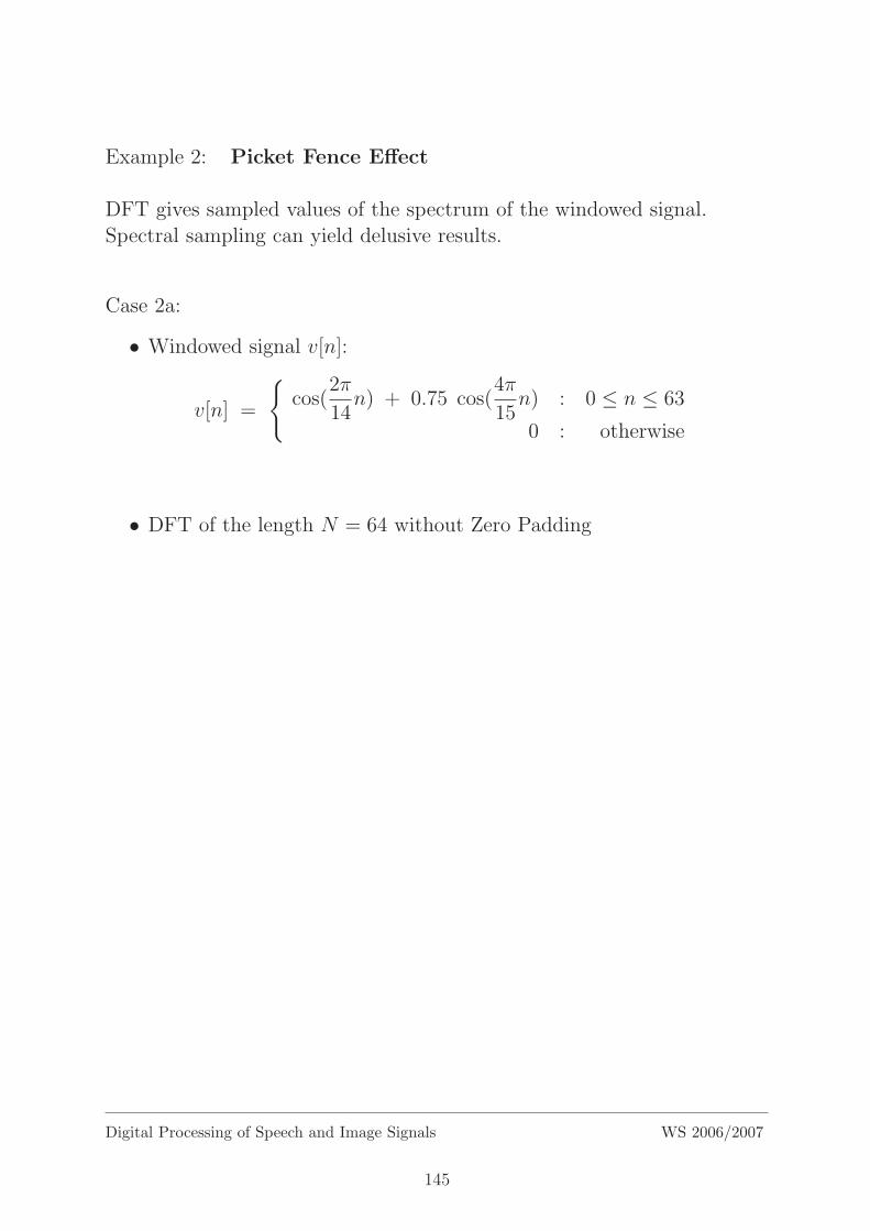
Example 2: Picket Fence Effect
DFT gives sampled values of the spectrum of the windowed signal.Spectral sampling can yield delusive results.
Case 2a:
• Windowed signal v[n]:
v[n] =
cos(
2π
14n) + 0.75 cos(
4π
15n) : 0 ≤ n ≤ 63
0 : otherwise
• DFT of the length N = 64 without Zero Padding
Digital Processing of Speech and Image Signals WS 2006/2007
145

a)
-1
0
1
2
63
n
v[n]
b)
0
30
V(k)
k63
c)
0
32
ωπ 2π
V(ω)
Figure 3.2: a) signal v[n]; b) DFT-spectrum V [k]; c) Fourier spectrum V (ejω).
Digital Processing of Speech and Image Signals WS 2006/2007
146

Case 2b:
• In contrast to case 2a, the frequencies of sinusoids are changed onlyslightly.
• Windowed signal v[n]:
v[n] =
cos(
2π
16n) + 0.75 cos(
2π
8n) : 0 ≤ n ≤ 63
0 : otherwise
• DFT of the length N = 64 without Zero Padding
Digital Processing of Speech and Image Signals WS 2006/2007
147

a)
-1
0
1
n
v(n)
63
b) 30
0 k
V(k)
63
c)
0
32
V(ω)
π 2π ω
Figure 3.3: a) signal v[n]; b) DFT-spectrum V [k]; c) Fourier spectrum V (ejω).
Digital Processing of Speech and Image Signals WS 2006/2007
148

Analysis of Example 2:
• The manifestation of the DFT can be put down to the spectral sam-pling. Although in Case 2b the windowed signal v[n] contains a sig-nificant number of frequencies beyond ω0 and ω1, they do not show inthe DFT spectrum of length N = 64.
• Using a rectangle window, the DFT of the sinusoidal signal gives sharpspectral lines, if the period N of the transformation is a whole multipleof the signal period and no Zero Padding is applied.
• Explanation for the case of a complex exponential function:
– Assume the signal x[n]:
x[n] =1
Nexp(j
2π
n0n)
– Then:
X[k] = δ(k − N
n0)
– For the DFT of rectangle window holds:
W [k] =sin(πk)
sin(πk/N)
– Convolution theorem for windowed signal v[n] gives:
V [k] = X[k] ∗ W [k] =
sin
(π(k − N
n0)
)
sin
(π(k − N
n0)/N
)
– In case of
N
n0∈ IN
only the DFT coefficient k =N
n0is non-zero.
Digital Processing of Speech and Image Signals WS 2006/2007
149

Example 2 (continued)
• Assume signal v[n] of Case 2b:
v[n] =
cos(
2π
16n) + 0.75 cos(
2π
8n) : 0 ≤ n ≤ 63
0 : otherwise
• In contrast to Case 2b, a DFT with length N = 128 is applied (Zero
Padding).
• Result:
Using finer sampling, existing additional frequency components emerge.
Digital Processing of Speech and Image Signals WS 2006/2007
150

a) 30
0 k
V(k)
63
b)
0 k127
V(k)
32
c)
0
32
V(ω)
π 2π ω
Figure 3.4: a) DFT of length N = 64; b) DFT of length N = 128; c) Fourier spectrumV (ejω).
Digital Processing of Speech and Image Signals WS 2006/2007
151

Example 3:
Explanation of following illustrations:
• Assume: signal of Example 2, Case 2a.
• Window: Kaiser window is applied instead of rectangle window.
• First: window length L = 64 and DFT length N = 64.
• Then: window length L and DFT length N are halved.
• Afterwards: for the case L = 32, the DFT length N is graduallyincreased up to N = 1024 (Zero Padding).
• Finally: DFT spectrum for the case N = 1024 and L = 64.
The Kaiser window is defined as:
wK [n] =
I0
[β(1− [(n− α) /α]2
)1/2]
I0(β): 0 ≤ n ≤ L− 1
0 : otherwise
In this example:
β = 0.8 and α =L− 1
2
The windowed signal v[n]:
v[n] = wK [n] cos(2π
14n) + 0.75 wK [n] cos(
4π
15n)
Digital Processing of Speech and Image Signals WS 2006/2007
152

Example 3: (continued)DFT length N = 64, window length L = 64
• Windowed signal
-1
0
1
n
v(n)
63
• DFT spectrum
30
0 k
V(k)
63
Digital Processing of Speech and Image Signals WS 2006/2007
153

Example 3: (continued)DFT length N = 32, window length L = 32
(N and L halved)
• Windowed signal
1
n310
v(n)
• DFT spectrum
8
V(k)
0 k31
Digital Processing of Speech and Image Signals WS 2006/2007
154

Example 3: (continued)
Effect of changing DFT length N at constant window length L = 32 (ZeroPadding)
• DFT length N = 32, window length L = 32
8
V(k)
0 k31
• DFT length N = 64, window length L = 32
8
V(k)
0 k63
Digital Processing of Speech and Image Signals WS 2006/2007
155
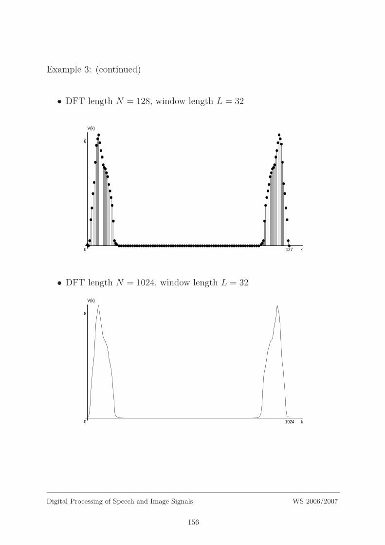
Example 3: (continued)
• DFT length N = 128, window length L = 32
8
V(k)
0 k127
• DFT length N = 1024, window length L = 32
8
V(k)
0 k1024
Digital Processing of Speech and Image Signals WS 2006/2007
156

Example 3: (continued)
Increasing the window length (L)
• DFT length N = 1024, window length L = 64
16
V(k)
0 k1024
Digital Processing of Speech and Image Signals WS 2006/2007
157

Example 4: Window function influence on the spectrum
0
0
speech signalphoneme "a"
0
amplitude spectrum- rectangle window -
0
amplitude spectrum- Hamming window -
Figure 3.5: Influence of the window function:above: speech signal (vowel “a”); central: 512 point FFT using rectangle window; below:512 point FFT using Hamming window
Digital Processing of Speech and Image Signals WS 2006/2007
158

3.3 Autocorrelation Function and Power Spectral Den-
sity
Definition of Autocorrelation Function (ACF) analog to the continuoustime case:
R[k] : =∞∑
n=−∞x[n] x[n+ k]
For a signal x[n] assume (e.g. after some suitable windowing):
x[n] =
x[n] 0 ≤ n ≤ N − 1
0 otherwise
In this case the ACF gives:
R[k] =N−1−k∑
n=0
x[n] x[n+ k] because x[n] = 0 for n < 0 and n ≥ N
“triangular effect”
N k-N
number of terms in R[k]
Cross correlation:
Rxy[k] =∞∑
n=−∞x[n] · y[n− k]
In contrast to convolution:
Oxy[k] =∞∑
n=−∞x[n] · y[k − n]
Digital Processing of Speech and Image Signals WS 2006/2007
159

Properties of ACF:
1. R[k] = R[−k]
2. R[k] ≤ R[0] for each k ∈ IN (R[0]: energy, intensity)
3. If x[n] −→ R[k], then αx[n] −→ α2R[k]
4. Intensity spectrum is the Fourier Transform of the ACF:
| X(ejω) |2 = X(ejω) ·X(ejω)
=∞∑
k=−∞x[k] exp(−jωk) ·
∞∑
l=−∞x[l] exp(jωl)
=∞∑
k=−∞
∞∑
l=−∞x[k] x[l] exp(−jωk) exp(jωl)
=∞∑
k=−∞
∞∑
l=−∞x[k + l] x[l] exp(−jωk) exp(−jωl) exp(jωl)
=∞∑
k=−∞
( ∞∑
l=−∞x[k + l] x[l]
)exp(−jωk)
=∞∑
k=−∞R[k] exp(−jωk)
Note: The phase spectrum is removed.
Digital Processing of Speech and Image Signals WS 2006/2007
160

5. Because of the symmetry R[k] = R[−k] the DFT becomes the cosinetransform:
| X(ejω) |2 =∞∑
k=−∞R[k] exp(−jωk)
=N−1∑
k=−(N−1)
R[k] exp(−jωk)
= R[0] +N−1∑
k=1
R[k] (exp(−jωk) + exp(jωk))
= R[0] + 2 ·N−1∑
k=1
R[k] cos(ωk) because R[k] = R[−k]
6. The intensity spectrum | X(ejω) |2 is a polynom of cos(ω) with gradeN − 1.
Reason: Moivre formula:
cos(ωk) = cosk(ω) −(k
2
)cosk−2(ω) sin2(ω) +
(k
4
)cosk−4(ω) sin4(ω) − . . .
Digital Processing of Speech and Image Signals WS 2006/2007
161

Example 1: Spectral analysis using ACF
0
0
speech signalphoneme "a"
0
amplitude spectrum- Hamming window -
0
amplitude spectrum- short hamming window -
0
amplitude spectrum- 19 ACF-coefficients -
0
amplitude spectrum- 13 ACF-coefficients -
Figure 3.6: Fourier Transform of a voiced speech segment:a) signal progression, b) high resolution Fourier Transform, c) low resolution FourierTransform with short Hamming window (50 sampled values), d) low resolution FourierTransform using autocorrelation function (19 coefficients), e) low resolution Fourier Trans-form using autocorrelation function (13 coefficients)
Digital Processing of Speech and Image Signals WS 2006/2007
162

Example 2: ACF of voiced and unvoiced speech segments
0
0
speech signalphoneme "a"
0
0
speech signalphoneme "s"
0
0
autocorrelation- rectangle window -
0
0
autocorrelation- rectangle window -
0
0
autocorrelation- Hamming window -
0
0
autocorrelation- Hamming window -
Figure 3.7: Signal progression and autocorrelation function of voiced (left) and unvoiced(right) speech segment
Digital Processing of Speech and Image Signals WS 2006/2007
163

Example 3: Temporal progression of autocorrelation coefficients
0
0
speech signal - digit sequence 0861909
0
ACF - coefficient for index 0 (energy)
0
0
ACF - coefficient for index 3
0
0
ACF - coefficient for index 6
0
0
ACF - coefficient for index 9
Figure 3.8: Temporal progression of speech signal and four autocorrelation coefficients
Digital Processing of Speech and Image Signals WS 2006/2007
164

3.4 Spectrograms
Using DFT
• Wide-band: in frequency domain:
– short time window
– “interaction” in the “synchronization” betweentime window and “pitch impulses”
– vertical lines
– no resolution of spectral fine structure
• Narrow-band: in frequency domain:
– long time window
– good resolution of the spectral fine structure
Digital Processing of Speech and Image Signals WS 2006/2007
165

Example 1: speech spectrograms
Figure 3.9: a) wide-band spectrogram: short time window, high time resolution (ver-tical lines), no frequency resolution; for voiced signals provides information on formantstructure b) narrow-band spectrogram: long time window, no time resolution, highfrequency resolution (horizontal lines); for voiced signals provides information on funda-mental frequency (pitch)
Digital Processing of Speech and Image Signals WS 2006/2007
166

Example 2: speech spectrograms
Figure 3.10: Wide-band and narrow-band spectrogram and speech amplitude for thesentence “Every salt breeze comes from the sea”.
Digital Processing of Speech and Image Signals WS 2006/2007
167

3.5 Filter Bank Analysis
• History:Decomposition of the signal using a “bank” of band-pass filters andenergy calculation in each frequency band
transferfunction
f
• Today digitally:
– Digital filters:
yk[n] =∞∑
m=−∞hk[n−m] x[m] , k = 1, . . . , K
– FIR: Finite Impulse ResponseIIR: Infinite Impulse Response (recursive filters)
– DFT (FFT) + further processing
• DFT/FFT Method:
– Window function
– Appending zeros for desired “resolution” (zero padding)
– FFT
– “Energy” calculation: |X(ejω)|, |X(ejω)|2, log |X(ejω)|– Weighted averaging for each channel and frequency band respec-
tively
Digital Processing of Speech and Image Signals WS 2006/2007
168

DFT/FFT filter bank:
transferfunction
f
transferfunction
f
Digital Processing of Speech and Image Signals WS 2006/2007
169

• Averaging:summation should be as smooth as possible over all channelsForm: rectangle, triangle, trapeze, etc.
• Choosing the central frequencies fk:
– constant:∆fk = const. for all ke.g. 20 channels with ∆f = 200Hz for 0− 4 kHz
– constant relative band width:
∆fkfk
= const. for all k
– frequency groups of the ear (total number 24):
f < 500Hz : ∆f = 100
f ≥ 500Hz :∆f
f= 20%
– adjusted to vowels or sounds
Digital Processing of Speech and Image Signals WS 2006/2007
170

3.6 Mel-frequency scale
The frequency resolution of the human ear is decreasing on the higherfrequencies. This empirical dependency results in the definition of the Melscale, which is approximately calculated as (from: Hidden Markov Toolkit,Cambridge University Engineering Departement, S.J.Young):
fMEL = 2595 log10 (1 +f
700Hz)
7000 f / Hz
2700
fMEL
Compression of the high frequencies
f
fMEL
A filter bank with constant band-widths can be used on the Mel scale:
fMEL
Digital Processing of Speech and Image Signals WS 2006/2007
171

Table: MEL Scale:
f/Hz fMEL
65 100136 200213 300298 400391 500492 600603 700724 800856 9001000 10001158 11001330 12001519 13001724 14001949 15002195 16002464 17002757 18003078 19003429 20003812 21004230 22004688 23005187 24005734 25006331 26006984 2700
Digital Processing of Speech and Image Signals WS 2006/2007
172

3.7 Cepstrum
The Cepstrum is the Fourier series expansion of the logarithm of the spec-trum.Comparison: autocorrelation function is a Fourier series of the normalspectrum.
We consider:
y[n] =∞∑
k=−∞h[n− k] x[k]
Goal:Separating the kernel h[n] from the input signal x[n].This problem is also called inversion or deconvolution.
• Convolution theorem:
Y (ejω) = H(ejω) X(ejω)
• Logarithm (complex):
logY (ejω) = logH(ejω) + logX(ejω)
• Inverse Fourier Transform:
F−1logY (ejω)
= F−1
logH(ejω)
+ F−1
logX(ejω)
Digital Processing of Speech and Image Signals WS 2006/2007
173

• Another notation:
y[n] = x[n] + h[n]
using the definition of the cepstrum for x[n](analogous for y[n] and h[n])
x[n] = F−1logX(ejω)
=1
2π
π∫
−π
exp(jωn) log X(ejω) dω
=1
2π
π∫
−π
exp(jωn) log
[∑
m
x[m] exp(−jωm)
]dω
= C x[n]
• Note:
– Cepstrum = artificial word derived from “spectrum”
– Cepstrum is located in time domain
Digital Processing of Speech and Image Signals WS 2006/2007
174

Through the cepstrum transformation
x[n] −→ x[n] = C x[n]
the convolution comes down to a simple addition.
In the cepstrum domain, a linear operation L (time invariance is not nec-essary) on y[n] is performed separately on h[n] and x[n]:
y[n] =∞∑
k=−∞h[n− k] x[k]
y[n] = h[n] + x[n]
L y[n] = Lh[n]
+ L x[n]
With the definitionGL for the concatenation of the cepstrum, the operationL, and the inverse cepstrum
GL := C−1 L C
we obtain
GL h[n] ∗ x[n] = GL h[n] ∗ GL x[n] .
Such a transformation GL acts on h[n] and x[n] separately, and is called:
homomorph (structure preserving)
Digital Processing of Speech and Image Signals WS 2006/2007
175

Complex cepstrum:
x[n] =1
2π
π∫
−π
exp(jωn) logX(ejω) dω
Note: complex logarithm
Simple cepstrum (real cepstrum):
x[n] =1
2π
2π∫
0
exp(jωn) log|X(ejω)| dω
• Cepstrum: Fourier coefficients of the logarithmized power spectraldensity
• ACF: Fourier coefficients of Fourier series of the power spectral density
Setting cepstral coefficients x[n] to zero for high n results in smoothing ofthe power spectral density.
Implementation:
Fourier Transform via N–FFT (N = 512, 1024, 2048)(But: discretisation error):
x[n] :=1
N
N−1∑
k=0
ej2π
Nkn
log |X(ej2π
Nk)|
Digital Processing of Speech and Image Signals WS 2006/2007
176

Example 1: Real cepstrum
Fine structure of power spectral density with the period 1/T results in asingle peak in the cepstrum at time T .
frequency
log|F(ω)|2
0 1T
F-1(log|F(w)|2)
time0 T
Figure 3.11: Above: logarithmized power spectrum of a spoken vowel (schematic).Below: corresponding cepstrum (inverse Fourier–transform of the logarithmized powerspectrum).
Digital Processing of Speech and Image Signals WS 2006/2007
177

Example 2: Smoothing
0
0
speech signalphoneme "a"
0
0
windowed phoneme "a"- Hamming window -
0
spectrum from cepstrum whole cepstrum
first 13 coefficients
Figure 3.12: Cepstral smoothing: speech signal (vowel “a”), windowed speech signal(Hamming window), spectrum obtained from the whole cepstrum (blue) and smoothedspectrum obtained from the first 13 cepstral coefficients (red).
Digital Processing of Speech and Image Signals WS 2006/2007
178

Example 3: Smoothing with different numbers of cepstral coefficients
0
0
speech signalphoneme "a"
0
spectrum from cepstrum whole cepstrum
first 13 coefficients
0
spectrum from cepstrum whole cepstrum
first 19 coefficients
0
spectrum from cepstrum whole cepstrum
first 19 coefficients first 13 coefficients
Figure 3.13: Homomorph analysis of a speech segment: signal progression, homomorphsmoothed spectrum using 13 and 19 cepstral coefficients
Digital Processing of Speech and Image Signals WS 2006/2007
179

Cepstrum calculation using Filter Bank Output
• Filter bank outputs A[k] for k = 1, . . . , KNote: k = 0 is missing.
• We complete the outputs symmetrically:
A A AA AA-K+1 -1 0 1 2 K
• Symmetry A−k+1 = Ak for all k = 1, . . . , K.
Digital Processing of Speech and Image Signals WS 2006/2007
180

Inverse DFT a[n] of the symmetric sequence A−K+1, . . . , AK :
a[n] =1
2K
K∑
k=−K+1
Ak exp
(2πj
2Knk
)
=1
2K
K∑
k=1
Ak
[exp
(2πj
2Knk
)+ exp
(2πj
2Kn(−k + 1)
)]
= exp
(2πj
2K0.5
)1
2K
K∑
k=1
Ak
[exp
(2πj
2Kn(k − 0.5)
)+ exp
(−2πj
2Kn(k − 0.5)
)]
= exp
(2πj
2K0.5
)1
K
K∑
k=1
Ak cos(πnK
(k − 0.5))
The phase term exp(
2πj2K 0.5
)depends on the position of the symmetry axis
around k = 0.5.
Cepstrum is defined as:
a[n] =1
K
K∑
k=1
Ak cos(πnK
(k − 0.5))
Digital Processing of Speech and Image Signals WS 2006/2007
181

Mel Cepstrum according to Davis and Mermelstein
ff = 100 f = 300
k = 1 k = 3 k = K
MEL MEL MEL
Filter bank:
• overlapping band-pass filters triangular shape,
• all channels have equal band width, and filter positioning is equidis-tant on a Mel scale.
Calculation of the filter bank outputs:
• magnitude of DFT coefficients,
• for each channel summation of the magnitudes according to triangularweight function,
• for each channel logarithm of the sum.
Thus the filter outputs A[k] with k = 1, . . . , K are obtained. Using thefilter bank outputs, the cepstrum is calculated using a cosine transform.(see previous description)
Digital Processing of Speech and Image Signals WS 2006/2007
182

3.8 Statistical Interpretation of the Cepstrum Trans-
formation
We consider the filter bank outputs log|Xk|.
s p kN/20
log |X |k
Assumption: The correlation between the outputs s and p, i.e. the elementCsp of the covariance matrix does not depend directly on s or p, but onlyon their difference. Because the spectrum is periodical there is no distancegreater than N :
Csp = c(s−p)modN
It is further assumed that the correlation is locally symmetric:
Cs,s+n = Cs,s−n
Then:c(s−s−n)modN = c(s−s+n)modN
c(−n)modN = c(+n)modN
With 0 ≤ n ≤ N follows:cn = cN−n
i.e. we have a symmetric cyclic matrix with the kernel vector c.
Digital Processing of Speech and Image Signals WS 2006/2007
183

Example: the covariance matrix for N = 8:
C =
c0 c1 c2 c3 c4 c3 c2 c1c1 c0 c1 c2 c3 c4 c3 c2c2 c1 c0 c1 c2 c3 c4 c3c3 c2 c1 c0 c1 c2 c3 c4c4 c3 c2 c1 c0 c1 c2 c3c3 c4 c3 c2 c1 c0 c1 c2c2 c3 c4 c3 c2 c1 c0 c1c1 c2 c3 c4 c3 c2 c1 c0
Such a covariance matrix will be diagonalised using the cosine transform(or Fourier Transform, which results in the cosine transform due to thesymmetry) (see excursion in chapter 2.17).
Digital Processing of Speech and Image Signals WS 2006/2007
184

3.9 Energy in acoustic Vector
The energy is usually added as zeroth (or first) component to the acousticvector.
For the logarithmic energy we have:
logE =1
2π
π∫
−π
log|X(ejω)|2 dω
For the (short time) spectrum or cepstrum it approximately holds:
logE ≈ 1
K
K∑
k=1
log|Xk|2
Spectra are usually normalized with log E:
logY 2k = log|Xk|2 − log E
such that:
K∑
k=1
logY 2k ≡ 0
The cepstral coefficient x[0] is the logarithmized energy.
Digital Processing of Speech and Image Signals WS 2006/2007
185

186

Chapter 4
Fourier Transform and ImageProcessing
• Overview:
4.1 Spatial Frequencies and Fourier Transform for Images
4.2 Discrete Fourier Transform for Images
4.3 Fourier Transform in Computer Tomography
4.4 Fourier Transform and RST Invariance
Digital Processing of Speech and Image Signals WS 2006/2007
187

4.1 Spatial Frequencies and Fourier Transform for
Images
A grey-valued image g(x, y) can be interpreted as:
g : IR2 → [0,∞[
(x, y) → g(x, y)
Space coordinates (x, y) are at first considered as continuous. Discretiza-tion and DFT will be analyzed later.
Convention: g(x, y) ≡ 0 outside of the image.
The Fourier–transform G(fx, fy) of the image g(x, y) is defined as:
G(fx, fy) = F(x, y)→ g(x, y)
=
∞∫
−∞
∞∫
−∞
g(x, y) e−2πj(fxx+fyy) dxdy
The arguments fx and fy are called spatial frequencies.
Digital Processing of Speech and Image Signals WS 2006/2007
188

The two-dimensional Fourier–transform can be obtained by using two one-
dimensional Fourier–transforms.We consider one “image row” with a constant value of y:
x → g(x, y)
Corresponding Fourier–transform Gy(fx) :
Gy(fx) = Fx → g(x, y)
=
∞∫
−∞
g(x, y) e−2πjfxx dx
Then we compute the Fourier–transform of the function:
y → Gy(fx)
and obtain:
Fy → Gy(fx) =
+∞∫
−∞
Gy(fx) e−2πjfyy dy
=
+∞∫
−∞
+∞∫
−∞
g(x, y) e−2πj(fxx+fyy) dxdy
In this way we get the result:
G(fx, fy) = Fy → Fx → g(x, y)
For the inverse FT we have (as can be expected):
g(x, y) = F−1(fx, fy) → G(fx, fy)
=
+∞∫
−∞
+∞∫
−∞
G(fx, fy) e2πj(fxx+fyy) dfxdfy
Digital Processing of Speech and Image Signals WS 2006/2007
189

We would like to interpret the two-dimensional FT visually. For this pur-pose, we consider the exponential factor in the FT and require the followingcondition:
e2πj(fxx+fyy) != 1
⇒ 2πj(fxx+ fyy) = 2πn for n ∈ IN
⇒ y = −fxfyx +
n
fy
y
x
∆Lθ
1/fy
1/fx
spatial period ∆L =1√
f 2x + f 2
y
Digital Processing of Speech and Image Signals WS 2006/2007
190

Special case:|G(fx, fy)| has a large value only at “one” point (u, v) = (fx, fy) in thespatial frequency plane
fx
fy
u-u
v
-v
|G(fx,fy)|
x
y
Digital Processing of Speech and Image Signals WS 2006/2007
191

Since G(fx, fy) = G(−fx,−fy) for a real image g(x, y), we have two
dominant frequency pairs in the Fourier–transform integral:
|G(u, v)| · [e2πj(ux+vy) + e−2πj(ux+vy)] = 2|G(u, v)| · cos 2π(ux+ vy)
This function describes a black-white cosine wave pattern with
(fx, fy) = (u, v)
Where is the value of G(fx, fy) large ?
ideally: points (u, v) and (−u,−v) represent cosine–variant of the greyvalues
really: straight line through (u, v) and (−u,−v) represents abrupt changes
of the grey values
Digital Processing of Speech and Image Signals WS 2006/2007
192

Figure 4.1: TV–image (analog) Figure 4.2: Digitized TV–image
Figure 4.3: Amplitude spectrum of Fig-ure 4.2
Figure 4.4: Low-pass filtered
Digital Processing of Speech and Image Signals WS 2006/2007
193
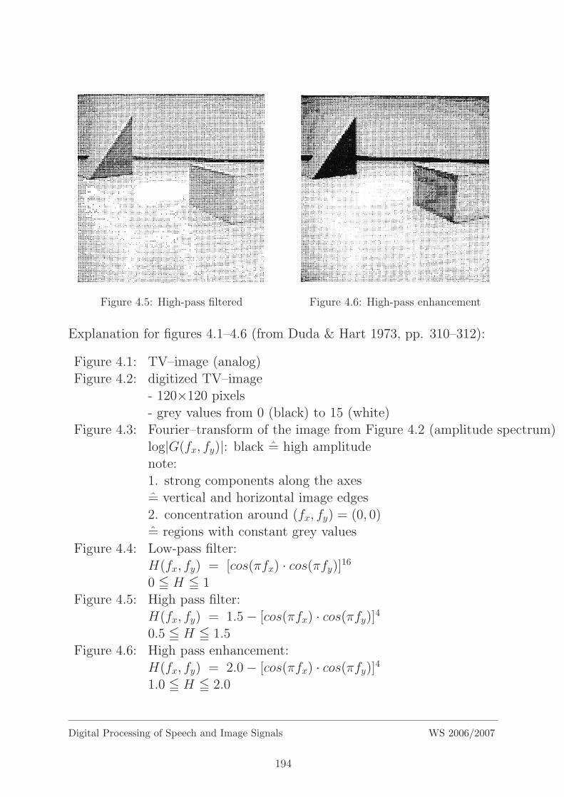
Figure 4.5: High-pass filtered Figure 4.6: High-pass enhancement
Explanation for figures 4.1–4.6 (from Duda & Hart 1973, pp. 310–312):
Figure 4.1: TV–image (analog)Figure 4.2: digitized TV–image
- 120×120 pixels- grey values from 0 (black) to 15 (white)
Figure 4.3: Fourier–transform of the image from Figure 4.2 (amplitude spectrum)log|G(fx, fy)|: black = high amplitudenote:1. strong components along the axes= vertical and horizontal image edges2. concentration around (fx, fy) = (0, 0)= regions with constant grey values
Figure 4.4: Low-pass filter:H(fx, fy) = [cos(πfx) · cos(πfy)]16
0 ≦ H ≦ 1Figure 4.5: High pass filter:
H(fx, fy) = 1.5− [cos(πfx) · cos(πfy)]40.5 ≦ H ≦ 1.5
Figure 4.6: High pass enhancement:H(fx, fy) = 2.0− [cos(πfx) · cos(πfy)]41.0 ≦ H ≦ 2.0
Digital Processing of Speech and Image Signals WS 2006/2007
194

Following general rules for G(fx, fy) ensue:
Edges in the image g(x, y):
• An image edge produces “strong” spatial frequency components alongone straight line in the spatial frequency plane which is orthogonal tothe edge.
• The “sharper” the edge is, the “longer” is the corresponding line inthe spatial frequency domain.
Regions with constant grey values:
• Regions with constant grey values increase the values of |G(fx, fy)|around the origin (fx, fy) = (0, 0). (fx, fy) = (0, 0) is called “DCcomponent” (average grey value, DC=direct current).
Digital Processing of Speech and Image Signals WS 2006/2007
195

4.2 Discrete Fourier Transform for Images
The analog image g(x, y) is discretized (“sampled”) along both axes. Weobtain the discrete image:
g[j, k] := g(j ·∆x, k ·∆y) where j, k = 0, 1, . . . , N − 1
Change in notation: i =√−1 instead of j
G(e2πiN·u, e
2πiN·v) =
N−1∑
j=0
N−1∑
k=0
g[j, k]e−2πiN
(uj + vk) where u, v = 0, 1, . . . , N − 1
Discretization is written as:
G[u, v] =N−1∑
j=0
N−1∑
k=0
g[j, k] e−2πiN
(uj + vk)
=N−1∑
j=0
e−2πiNuj·(
N−1∑
k=0
g[j, k] e−2πiNvk
)
Interpretation:Fourier–transform of the image is first performed row by row, then columnby column.Using usual definition of the “Fourier matrix” W (i.e. Wvk = (e−
2πiN )vk),
we obtain the matrix representation of Fourier–transform.
Using the notation:g ∈ IRNxN
W ∈ CNxN
G ∈ CNxN
we obtainG = [W g W ]
g =1
N 2· [W−1 GW−1]
Note: In the corresponding definition of the Fourier–transform, instead ofthe factors 1 and 1/N 2 we have the factors 1/N and 1/N or 1/N 2 and 1.
Digital Processing of Speech and Image Signals WS 2006/2007
196

4.3 Fourier Transform in Computer Tomography
y=ax+b,a const.
x
yb
We consider a projection of the image g(x, y) along the straight line:
y = ax + b
We produce a set of straight lines by keeping a constant and varying b.
Projection:
ga(b) =
∫g(x, ax+ b) dx
Fourier–transform:
Ga(fb) =
∫ga(b) e
−2πjfbb db
=
∫ ∫g(x, ax+ b) e−2πjfbb db dx
We substitute b = y − ax and obtain:
Ga(fb) =
∫ ∫g(x, y) e−2πj(yfb−xafb) dydx
= G(−afb, fb)= Fourier–transformG(fx, fy) of g(x, y) along
the spatial frequency straight line (fx, fy) with fy = −1
afx
Digital Processing of Speech and Image Signals WS 2006/2007
197

Remarks:
a. Straight line in spatial frequency domain: (fx, fy) = (−afb, fb) isorthogonal to y = ax + b:
y = ax + b => in Fourier–transform fy = −1
afx
The angle between these straight lines is a right angle becausea·(−1a
)= −1.
In general:
y1(x) = m1 x + b1
y2(x) = m2 x + b2
y1(x) ⊥ y2(x) ⇔ m1 ·m2 = −1
b. The value Ga(fb) is independent of the “offset” b and depends onlyon the orientation a of the straight line. Therefore, if we calcu-late the projection for many different inclinations a and apply theone-dimensional FT, we obtain the two-dimensional FT of the imageg(x, y).
Digital Processing of Speech and Image Signals WS 2006/2007
198

4.4 Fourier Transform and RST Invariance
We will investigate invariance of the Fourier–transform to
R : Rotation
S : Scaling
T : Translation
We will use vector notation for the two-dimensional Fourier–transform:
coordinates: z =
(x
y
)∈ IR2
image grey values: g(z) = g(x, y) ∈ IR+
spatial frequency: f =
(fxfy
)∈ IR2
We ignore the discretization.
Digital Processing of Speech and Image Signals WS 2006/2007
199

Translation
z → z + z0
with translation vector z0 =
(x0
y0
)∈ IR2
Image : g(z) → g(z) := g(z + z0)
FT : G(f) = exp (i[fxx0 + fyy0]) ·G(f)
Rotation
z → Dϑz
with rotation matrix Dϑ =
[cosϑ sinϑ− sinϑ cosϑ
]
y
x
ϑ
Digital Processing of Speech and Image Signals WS 2006/2007
200

Scaling
z → α · zwith scaling factor α > 0
Image : g(z) → g(z) = g(α · z)
FT : G(f) =1
α2· G
(f
α
)
basically: similarity principle (S.??) for one-dimensional FT
transferred to two dimensions
Invertible linear mapping
z → A · zwhere A ∈ IR2×2 invertable
Image : g(z) → g(z) = g(Az)
FT : G(f) = . . .
=1
det(A)· G((A−1)Tf)
Proof: transformation of two-dimensional integration variables
Digital Processing of Speech and Image Signals WS 2006/2007
201

We apply two basic rules to obtain the RST-invariance:
1. Invariance to translation (=T) can be obtained by using the square ofthe absolute value
g(z) → G(f) → |G(f)|2
2. To obtain RS-invariance we transfer to polar coordinates in the spatialfrequency domain. We write in complex notation:
fz ≡ fx + i fy = r eiφ = exp (ln r + iφ) ∈ C2
Complex logarithm:f ′z := ln fz = ln r + iφ
We already know:
a) rotation by angle φ0 in spatial domain= rotation by angle φ0 in spatial frequency domain
b) scaling with factor α in spatial domain
= scaling with factor( 1
α
)and
( 1
α
)2
respectively in spatial
frequency domain
f ′zscaling and−→
rotationf ′z
Digital Processing of Speech and Image Signals WS 2006/2007
202

f ′z = ln z
= ln r + iφ
= ln( r
α
)+ i(φ − φ0)
= ln r + i φ − ln α − i φ0
= f ′z − lnα − i φ0
= translation with the shift vector (− ln α − i φ) ∈ C2
in logarithmic polar coordinates of the spatial frequency plane
Digital Processing of Speech and Image Signals WS 2006/2007
203

RST-invariant features can therefor be obtained as follows:
g(x, y) image: (x, y) ∈ IR2
first Fourier–transform
G(fx, fy) = Fg(x, y) mit (fx, fy) ∈ IR2
squared absolute value
|G(fx, fy)|2
logarithmic polar coordinates: (ln r, φ)
|G(ln r, φ)|2
second Fourier–transform
F (|G(ln r, φ)|2)
squared absolute value
|F (|G(ln r, φ)|2)|2
Next page:Analysis of the RST-invariant features.Original grey valued images are identical up to a 90–rotation.
Digital Processing of Speech and Image Signals WS 2006/2007
204

original image-
6
x
y
|FFT|-
6
fx
fy
log–polar-
6
ln r
φ
|FFT|-
6
fx
fy
Digital Processing of Speech and Image Signals WS 2006/2007
205

Warning:
a) Invariant observations are not necessarily good for classification.
b) Observations that are calculated using the two-dimensional Fourier–transform are not complete, i.e. the original image cannot be recon-structed completely.
Digital Processing of Speech and Image Signals WS 2006/2007
206

Chapter 5
LPC Analysis
• Overview:
5.1 Principle of LPC Analysis
5.2 LPC: Covariance Method
5.3 LPC: Autocorrelation Method
5.4 LPC: Interpretation in Frequency Domain
5.5 LPC: Generative Model
5.6 LPC: Alternative Representations
The acronym LPC stands for
Linear Predictive Coefficients / Coding
and is utilized in signal processing and frequency analysis, as well as insignal coding.
Digital Processing of Speech and Image Signals WS 2006/2007
207

5.1 Principle of LPC Analysis
timenn-2
We consider a discrete time signal x[n], possibly multiplied with a windowfunction. The goal of an LPC analysis is to predict each signal value x[n]by its preceding values x[n− 1], x[n− 2], ..., x[n−K]. We distinguish:
x[n] : signal value
x[n] : predicted value
We assume the predicted value x[n] to be a linear combination of thepreceding values of x[n]:
x[n] :=K∑
k=1
αk x[n− k]
with at first unknown coefficients αk, k = 1, ..., K, which are called
LPC–coefficients or prediction coefficients.
The value K is called prediction order, e.g. K = 8, . . . , 10 at a samplingfrequency of 4 kHz (about 2 coefficients per kHz).
Digital Processing of Speech and Image Signals WS 2006/2007
208

Outlook
Starting point: “coding” in time domain (goal: bit reduction)
↓ Parseval Theorem
parametric model for power spectrum of Fourier–transform(more exact: rough structure of power spectrum for speech signal)
LPC analysis applications:
• speech coding(ADPCM = adaptive differential pulse code modulation)
• signal processing:parametric modelling with autoregressive or all-pole models (order K)
• time curves:resonance and oscillator curves, sun spots, stock-market course, ...
• image coding
• also: interpretation as Maximum Entropy Approach
Digital Processing of Speech and Image Signals WS 2006/2007
209

The coefficients αk are unknown at first. To estimate these, we define theprediction error for each point n in time:
e[n] := x[n]− x[n]
= x[n]−K∑
k=1
αk x[n− k]
For a reliable set of LPC–coefficients we calculate the squared error crite-rion E as sum of the squared prediction errors e[n]:
E =∑
n
e2(n)
=∑
n
[x[n]−
K∑
k=1
αk x[n− k]]2
!= minimum with respect to α1, . . . , αk, . . . , αK
Taking the derivative ∂∂αl
for l = 1, . . . , K results in:
∑n
(x[n]−∑
k
αk x[n− k])x[n− l] !
= 0
∑k
αk∑nx[n− k]x[n− l] =
∑nx[n− l]x[n]
Here, the summation limits are not specified on purpose.If the squared error criterionE is considered as a function of LPC–coefficients,the following properties ensue:
• E is quadratic in α1, . . . , αk, . . . , αK ; it is guaranteed to be non-negative and it has a single well-defined minimum.
• The optimal LPC–coefficients are invariantto linear scaling of the signal values x[n].
Digital Processing of Speech and Image Signals WS 2006/2007
210

Minimization of the squared error criterion with respect to the LPC–coefficients results either from taking the derivative or from the “quadraticcomplement” (recalculate for yourself!). The linear equation system forthe LPC–coefficients αk ensues:
l = 1, . . . , K :K∑k=1
αk ·∑nx[n− k] x[n− l] =
∑
n
x[n− l] x[n]
with still unspecified summation limits over n. We consider two methodsfor the choice of summation limits:
1. covariance method
2. autocorrelation method
Warning: terminology is not consistent.
Digital Processing of Speech and Image Signals WS 2006/2007
211

5.2 LPC: Covariance Method
n0 N-1
known values predicted value
Covariance Method
• No window function is applied, such that we obtain the followingsummation limits:
∑
n
e2(n) =N−1∑
n=0
e2(n)
i.e. we also use signal values x[n] with n < 0 for prediction.
• The resulting equation system for LPC–coefficients:
l = 1, . . . , K :K∑
k=1
αk Φ(l, k) = Φ(l, 0)
with the definition:
Φ(l, k) :=N−1∑
n=0
x[n− l] x[n− k]
For the above terms hold:
– they describe a kind of cross correlation between two “signals”
– they are similar to a covariance matrix
Computational complexity for solving the equation system:
O(K3) + O(NK)
– autocorrelation method has more favorable complexity: O(K2)
– but: calculation of auto/cross-correlation function dominates
In contrast to covariance method, autocorrelation method offers an inter-pretation in the frequency domain and therefore is often preferred.
Digital Processing of Speech and Image Signals WS 2006/2007
212

5.3 LPC: Autocorrelation Method
n0 N-1
windowfunction
We consider the signal after multiplication with a convenient window func-tion, usually Hamming window:
In principle, the summation limits now are
∑
n
e2[n] =n=+∞∑
n=−∞e2[n] .
Since, due to windowing the signal x[n] is identical to zero outside thewindow function, i.e.
x[n] ≡ 0 for n < 0 or N − 1 < n
we obtain the following for the prediction error e[n]:
e[n] ≡ 0 for n < 0 or N − 1 +K < n
Therefore, the total error E becomes:
E =N+K−1∑
n=0
e2[n]
The prediction error e[n] can become “large” on the window functionboundaries:
- Beginning: prediction from ”zeros”- End: prediction of ”zeros”
Digital Processing of Speech and Image Signals WS 2006/2007
213

Inserting the summation limits:∑
n
x[n− k] x[n− l] = R(|l − k|),∑
n
x[n] x[n− l] = R(|l|)
where R(|l − k|) =N−1−l∑
n=0
x[n− k] x[n− l]
R(|l|) =∑
n
x[n] x[n− l] =N−1−l∑
n=0
x[n] x[n− l]
In this way we obtain the following equation system for the LPC–coefficientsαk:
l = 1, ..., K :K∑
k=1
αkR(|l − k|) = R(l)
or in matrix form:
R(0) R(1) . . . R(K − 1)
R(1) R(0) . . . R(K − 2)
......
. . . ...
... R(1)
R(K − 1) R(K − 2) . . . R(1) R(0)
α1
α2
...
αK
=
R(1)R(2)
...
R(K)
Digital Processing of Speech and Image Signals WS 2006/2007
214

Note that this equation system is completely determined by the autocor-relation coefficients
R(0), ..., R(k), ..., R(K).
Hence, the autocorrelation coefficients will “only” be converted to obtainthe LPC–coefficients
α1, ..., αk, ..., αK .
The matrix of this equation system has the following properties:- Toeplitz structure (follows from time invariance)- solution: Durbin–algorithm with complexity O(K2)
Digital Processing of Speech and Image Signals WS 2006/2007
215

5.4 LPC: Interpretation in Frequency Domain
The LPC autocorrelation method allows prediction error conversion fromtime domain into frequency domain using Parseval theorem so that LPCanalysis can be interpreted as adaptation of parametric model spectrum tothe observed signal spectrum.We start with the prediction error e[n]:
e[n] = x[n]−K∑
k=1
αk x[n− k]
and apply the z–transform to this equation. The z–transform is restrictedto the unit circle.
z = ejω ∈ C
For the z-transforms E(z) and X(z) we obtain:
E(z) = X(z) ·[1−
K∑
k=1
αkz−k]
The total error Etot for the squared error criterion becomes:
Etot =N+K−1∑
n=0
e2[n]
=1
2π
+π∫
−π
|E(ejω)|2 dω (Parseval Theorem)
=1
2π
+π∫
−π
∣∣∣∣∣1−K∑
k=1
αk e−jωk
∣∣∣∣∣
2
· |X(ejω)|2 dω
=1
2π
+π∫
−π
∣∣P (ejω)∣∣2 · |X(ejω)|2 dω
Digital Processing of Speech and Image Signals WS 2006/2007
216

with the so-called predictor polynom:
P (ejω) := 1−K∑
k=1
αk e−jωk
Squared absolute value of the predictor polynom
∣∣P (ejω)∣∣2 =
∣∣∣∣∣1−K∑
k=1
αk e−jωk
∣∣∣∣∣
2
= ...
=K∑
k=1
Bk · cos(ωk)
(with suitable coefficients Bk resulting from the predictor coefficients) is apolynom with respect to cos(ω), which can be obtained via application oftrigonometric transformations.
The predictor polynom tries to “compensate” for |X(ejω)|2 – especially atmaxima – and to generate a “white” spectrum for the prediction error e[n].
The complex predictor polynom P (z) with z ∈ C has exactly K zeros inthe complex plane and therefore can be factorised into linear factors:
P (z) =K∏
k=1
(z − zk)
Digital Processing of Speech and Image Signals WS 2006/2007
217

Observations:
• These zeros are complex conjugated pairs because αk ∈ IR.
• The zeros can cause ”minima” of∣∣P (ejω)
∣∣2. The minima of |P (ejω)|2approximately correspond to the maxima of the smoothed spectrum|X(ejω)|2, because for minimization of the error integral it is first ofall necessary to “compensate” for the maxima of the signal spectrum.The LPC analysis could therefore be used to describe of the speechsignal formant structure.
|P(e )|2iω
ω
|X(e )|2iω
Digital Processing of Speech and Image Signals WS 2006/2007
218

0
0
windowed phoneme "a"- Hamming window -
0
0
prediction error- 12 LPC-coefficients -
0
LPC-spectrum- 12 coefficients -
0
spectrum ofprediction error
(12 LPC-coefficients)
0
LPC-spectrum- 18 coefficients -
Figure 5.1: LPC–analysis of one speech segmenta) signal progression, b) prediction error (K=12), c) LPC–spectrum with K=12 coeffi-cients, d) spectrum of the prediction error (K=12), e) LPC–spectrum with K=18 coeffi-cients
Digital Processing of Speech and Image Signals WS 2006/2007
219

0
0
windowed phoneme "a"- Hamming window -
0
amplitude spectrum- Hamming window -
0
LPC-spectrum- 4 coefficients -
0
LPC-spectrum- 8 coefficients -
0
LPC-spectrum- 12 coefficients -
0
LPC-spectrum- 16 coefficients -
0
LPC-spectrum- 18 coefficients -
0
LPC-spectrum- 20 coefficients -
Figure 5.2: LPC–Spectra for different prediction orders K
Digital Processing of Speech and Image Signals WS 2006/2007
220

5.5 LPC: Generative Model
e(n) x(n)
recursivefilter
αk
For the prediction error e[n] and its z–transform holds:
e[n] = x[n]−K∑
k=1
αk x[n− k]
E(z) = X(z)−K∑
k=1
αk X(z) z−k
= X(z) · [1−K∑
k=1
αk z−k]
If we consider prediction error as input signal, we can also interpret theLPC–theorem as generative model which generates an output signal x[n]from an adequate “input signal” e[n]:
x[n] = e[n] +K∑
k=1
αk x[n− k] .
For the signal spectrum X(z) holds:
X(z) =E(z)
1−K∑k=1
αk z−k
This model is called autoregressive model. The excitation has to be chosensuch that E(z) is “white”, i.e. it does not have fine structure due to thefundamental frequency (”pitch–frequency”).In other words:
E(z) = G = const. (”gain”)
Digital Processing of Speech and Image Signals WS 2006/2007
221

Special case:
E[n] = G · δ[n]
Then for LPC model spectrum X(z) holds:
X(z) =G
1−K∑k=1
αk z−k
This spectrum is often interpreted as LPC model spectrum X(z) of ob-served signal. It is reasonable to set (without explanation):
G2 = R(0)−K∑
k=1
αk R(k) = R(0)
[1−
K∑
k=1
αkR(k)
R(0)
]
This LPC model spectrum does not have any zeros, it has only poles, andtherefore is also called all–pole model.
Remarks:
• stability problems by solving the equation system
(←− truncation error in autocorrelation)
• way out: preemphasis through difference calculation
• absolute rule for choice of order K:
1 formant needs 2 LPC–coefficients
1 formant per kHz
+ excitation pulse shape + radiation: 2 LPC–coefficients
=⇒ rule of thumb:
bandwidth
4 kHz K = 105 kHz K = 126 kHz K = 14
Digital Processing of Speech and Image Signals WS 2006/2007
222

5.6 LPC: Alternative Representations
• so far:
G gainαk LPC–coefficients
• impulse response of generative model
• impulse response of squared absolute value of ”predictor polynom”
• cepstrum
• poles / zeros of synthesis model / ”predictor polynom”
=⇒ formants / bandwidths
problem: noise susceptible
• PARCOR–coefficients: partial correlation
• Area–coefficients: cross-section surfaces Ak
• reflexion coefficients ∼ PARCOR; tube model
A1 A2 A3 A4 A5
Glottis Lips
Digital Processing of Speech and Image Signals WS 2006/2007
223


Chapter 6
Outlook: Wavelet Transform
• Overview:
6.1 Motivation: from Fourier to Wavelet Transform
6.2 Definition
6.3 Discrete Wavelet Transform
Digital Processing of Speech and Image Signals WS 2006/2007
225

6.1 Motivation: from Fourier to Wavelet Transform
Fourier transform uses infinitely extended basis functions
e−jωt
and therefore does not have any time resolution, i.e. there is no informa-tion about the localization along the time axis.
Therefore, a window function often is used
t → w(t), complex in general
This function has finite support such that it is possible to investigate asegment of a function of interest.
We define a short–time Fourier transform Fb(w) of time signal t → f(t)at position b ∈ IR in time:
Fb(w) :=
+∞∫
−∞
f(t)w(t− b)e−jωt dt
where w(t) denotes the complex conjugated value of w(t).
The wavelet–transform can be derived from this equation in two steps:
a) we ignore the basis function e−jωt and we define the window functionas the new basis function.
b) in addition to the localization parameter b, we also introduce a scaling
parameter a > 0.
We consider the family of window functions Wab(t):
wab(t) := w( t− b
a
)
Digital Processing of Speech and Image Signals WS 2006/2007
226

6.2 Definition
The following notation is usually used for the Wavelet–transform:
ψab(t) :=1√a· ψ(t− ba
)
which is the so-called Mother-Wavelet t→ ψ(t).
Like the window function for the short–time Fourier transform the Mother-Wavelet should be “localized” as much as possible.
Example:
Mexican-Hat Function: ψ(t) = (1− t2)e− 1
2t2
t
ψ (t)
Digital Processing of Speech and Image Signals WS 2006/2007
227

The wavelet–transform of f(t) with respect to ψ(t) is defined as:
Fψ(a, b) =1
a
+∞∫
−∞
f(t) · ψ( t− b
a
)dt
with scaling parameter a > 0 and localization parameter b ∈ IR.
For the inverse transformation holds:
f(t) =1
Cψ· 1
a2·
+∞∫
0
da
+∞∫
−∞
db Fψ(a, b) · ψ( t− b
a
)
with
Cψ :=
∞∫
0
|ψ(ω)|2ω
dω < ∞
Proof (principle only):
The proof uses the (generalized) Parseval Theorem:
Fψ(a, b) =1√a
+∞∫
−∞
f(t) · ψab(t) dt
=1√a
+∞∫
−∞
F (ω) · ψab(ω) dω
with ψab(t) =1√a· ψ(t− ba
)
using further conversions.
Digital Processing of Speech and Image Signals WS 2006/2007
228

6.3 Discrete Wavelet Transform
For the scaling parameters a > 0 we choose:
a = αm0 where α0 > 1 and m ∈ Z.
The values of m determine the width of wavelet ψab(t).
In order to adjust the localization parameter properly, we define:
b = n b0 am0 where b0 > 0 and n ∈ Z.
Thus we constrain the Wavelet transform to discrete values :
Fψ(a, b) → Fψ(n,m)
The choice of the function ψ(t) is still open.
It is useful to choose ψ(t) such that the function system ψmn|m,n ∈Z, m > 0
with ψmn(t) := a−m
2
0 · ψ(a−m0 t − nb0)
represents an orthonormal basis for functions t→ f(t) ∈ L2(IR).
Note: The scalar product < f(t), g(t) > of two functions f(t) and g(t) isdefined as:
< f(t), g(t) > =
∫f(t) · g(t) dt
Digital Processing of Speech and Image Signals WS 2006/2007
229

In this way we obtain the following representation for the discrete Wavelet–
transform:
Fψ(m,n) =
+∞∫
−∞
f(t)a−m
2
0 ψ(a−m0 t − nb0) dt
= < f(t), ψmn(t) >
Due to the orthogonality it is possible to convert the integral of the inverseWavelet–transform into an infinite series:
f(t) =1
Cψ
∑
m
∑
n
Fψ(m,n)ψmn(t)
=1
Cψ
∑
m
∑
n
Fψ(m,n) a−m
2
0 ψ(a−m0 t − nb0)
Digital Processing of Speech and Image Signals WS 2006/2007
230

Example: Haar–function and Haar–basis
special choice: a0 = 2b0 = 1
The Haar–function is defined as:
ψ(t) =
1 0 ≦ t ≦ 12
−1 12 ≦ t < 1
0 otherwise
This defines the Haar–basisψ(t) |m,n ∈ Z,m > 0
:
ψmn(t) =1√2m· ψ
(2mt − n
)
It is easy to see that for increasing m a increasingly finer resolution is ob-tained and that n determines localization in time.
Digital Processing of Speech and Image Signals WS 2006/2007
231

Digital Processing of Speech and Image Signals WS 2006/2007
232

Chapter 7
Coding
The following types of coding are distinguished:
• source coding (data compression)goal: transmission (storage) using as few bits as possible without or
with few errors
• channel codinggoal: preferably faultless data transmission (storage)e.g. error-recognizing and error-correcting codes
• simultaneous source and channel codinggoal: simultaneous optimization
The following data types are distinguished:
• discrete alphabet
• continuous signal (audio, video, . . . )
Source coding
• lossless coding (compression)usually discrete sources, e.g. text compression
• lossy codingusually continuous signalsnotation:rate - distortion theory
distortion, error
bit rate
233

Digital Processing of Speech and Image Signals WS 2006/2007
234

Three effects can be utilized for signal coding:
a) statistical redundancy and correlation:samples are not independent.
b) perceptive properties of the receiver (ear and eye):some fine structures in the signal are irrelevant to the receiver
c) signal distortion:coded signal differs from the original signal without significant qualitydeterioration.
signal
reconstructedsignal
T Q C
T Q C-1 -1 -1
trans-mission
T: transformation, e.g. DCT
Q: quantization, e.g. vector quantization
C: mapping of bit representation
Digital Processing of Speech and Image Signals WS 2006/2007
235

References:
• Ze-Nian Li: CMPT 365 Multimedia Systems. Simon FraserUniversity, British Columbia, Canada, fall 1999, Version Jan.2000;
http://www.cs.sfu.ca/CourseCentral/365/li/index_prev.html.
• Peter Noll: MPEG Digital Audio Coding. IEEE Signal ProcessingMagazine, pp.59-81, Sep. 1997.
• Thomas Sikora: MPEG Digital Video-Coding Standards. IEEE SignalProcessing Magazine, pp.82-100, Sep. 1997.
• A. Ortega, K. Ramchandran: Rate-Distortion Methods for Imageand Video Compression. IEEE Signal Processing Magazine, pp.23-50, Nov. 1998.
• G. J. Sullivan, Th. Wiegand: Rate-Distortion Optimization for VideoCompression. IEEE Signal Processing Magazine, pp.74-90, Nov. 1998.
Digital Processing of Speech and Image Signals WS 2006/2007
236

Chapter 8
Image Segmentation andContour-Finding
The lecture notes for this chapter are available as a separate document.
237

238