Digital Transmitters D2000 Series - OMEGA Engineering · Digital Transmitters MADE IN ... Tel: +31 (0)20 3472121 FAX: +31 (0)20 6434643 Toll Free in Benelux: 0800 0993344 ... 1000

omega.com e-mail: [email protected]

For latest product manuals:omegamanual.info

User’s Guide

D2000 SeriesDigital Transmitters

MADE IN

Shop online at

Servicing North America:U.S.A.: One Omega Drive, Box 4047ISO 9001 Certified Stamford, CT 06907-0047

Tel: (203) 359-1660 FAX: (203) 359-7700e-mail: [email protected]

Canada: 976 BergarLaval (Quebec) H7L 5A1, CanadaTel: (514) 856-6928 FAX: (514) 856-6886e-mail: [email protected]

For immediate technical or application assistance:U.S.A. and Canada: Sales Service: 1-800-826-6342 / 1-800-TC-OMEGA®

Customer Service: 1-800-622-2378 / 1-800-622-BEST®

Engineering Service: 1-800-872-9436 / 1-800-USA-WHEN®

Mexico: En Espanol: (001) 203-359-7803 e-mail: [email protected]: (001) 203-359-7807 [email protected]

Servicing Europe:Benelux: Postbus 8034, 1180 LA Amstelveen, The Netherlands

Tel: +31 (0)20 3472121 FAX: +31 (0)20 6434643Toll Free in Benelux: 0800 0993344e-mail: [email protected]

Czech Republic: Frystatska 184, 733 01 Karvina , Czech RepublicTel: +420 (0)59 6311899 FAX: +420 (0)59 6311114Toll Free: 0800-1-66342 e-mail: [email protected]

France: 11, rue Jacques Cartier, 78280 Guyancourt, FranceTel: +33 (0)1 61 37 2900 FAX: +33 (0)1 30 57 5427Toll Free in France: 0800 466 342e-mail: [email protected]

Germany/Austria: Daimlerstrasse 26, D-75392 Deckenpfronn, GermanyTel: +49 (0)7056 9398-0 FAX: +49 (0)7056 9398-29Toll Free in Germany: 0800 639 7678e-mail: [email protected]

United Kingdom: One Omega Drive, River Bend Technology CentreISO 9002 Certified Northbank, Irlam, Manchester

M44 5BD United Kingdom Tel: +44 (0)161 777 6611 FAX: +44 (0)161 777 6622Toll Free in United Kingdom: 0800-488-488e-mail: [email protected]

OMEGAnet® Online Service Internet e-mailomega.com [email protected]

It is the policy of OMEGA Engineering, Inc. to comply with all worldwide safety and EMC/EMIregulations that apply. OMEGA is constantly pursuing certification of its products to the European NewApproach Directives. OMEGA will add the CE mark to every appropriate device upon certification.The information contained in this document is believed to be correct, but OMEGA accepts no liability for anyerrors it contains, and reserves the right to alter specifications without notice.WARNING: These products are not designed for use in, and should not be used for, human applications.

Omega EngineeringOne Omega DriveP O Box 4047Stamford, CT 06907Phone: 1-800-DAS-IEEEFax: 203-359-7990e-mail: [email protected]

D2000 SERIESPROGRAMMING MANUAL

REVISED 10/27/04

TABLE OF CONTENTS

CHAPTER 1 Linear Scaling 1-1Nonlinear Functions 1-3

CHAPTER 2 Block Diagram 2-2Programming Table 2-3Breakpoints 2-7

CHAPTER 3 BreakPoint Command 3-1MiNimum Command 3-2MaXimum Command 3-2

CHAPTER 4 Programming Software 4-1General Guidelines 4-1Function Programming 4-4Linear Scaling 4-7

CHAPTER 5 Programming Steps 5-3Examples 5-6

Chapter 1Introduction

The D2000 series of intelligent analog-to-computer interfaces are designedto solve many difficult interfacing problems that cannot be performed withexisting standard interfaces. The D2000 series may be programmed tocreate custom transfer functions to interface to non-standard sensors or toscale the outputs to any engineering units desired.

The D2000 series is an enhancement of the D1000 series of standardinterfaces. The D2000 series is similar to the D1000 series in every respectexcept that the D2000 interfaces allow custom input-to-output transferfunctions. As shipped from the factory, the D2000 modules operate in thesame manner as their D1000 counterparts. For example, a D2111 shippedfrom the factory contains the same transfer function as a D1111 module; inthis case they are both ±100 mV inputs and communicate with RS-232.Before any attempt is made to program a D2000, you must first be familiarwith the operation of a D1000 module as described in the D1000 manual.

The D2000 contains built-in commands to create custom functions. Allprogramming is performed through the communications port of the D2000module. There is never any need to open the module case. Modules may bere-ranged remotely as many times as desired. Transfer function data valuesare stored in nonvolatile memory to retain the scaling even if power isremoved.

Linear ScalingThe basic concept of the D2000 series is to create interfaces which outputdata in application specific engineering units that may be instantly read andinterpreted without any data conversion necessary by a host computer. Infact, the D2000 interfaces may be used with a dumb terminal to provide datareadings in easy-to-understand engineering units. For example, a typicalpressure sensor might provide a 1 to 5V. linear output for pressures of 0 to1000 psi. Using a D1131 module or an unprogrammed D2131 unit the outputdata would look like this:

Pressure (psi) Sensor Output D2131 Output (mV)

0 1V +01000.00500 3V +03000.001000 5V +05000.00

The standard output of the D2131 reads out in units of millivolts. Even thoughthe D2131 will faithfully output the sensor voltage, the real parameter ofinterest is pressure, not voltage, and the voltage readings may be difficult to

Introduction (1-2)

interpret. To make the output data more readable, the D2131 may beprogrammed to output the data values in units of pressure:

Pressure (psi) Sensor Output D2131 Output (psi)

0 1V +00000.00500 3V +00500.001000 5V +01000.00

In some cases, the desired output may be more specific to a particularapplication. Assume that the same pressure sensor is used to measure the“fullness” of a pressure vessel, such as a cylinder of compressed air. TheD2131 could be scaled to output in units of “percent” and in this case we willassume that if the cylinder reads 750 psi it is 100% full:

Pressure Volts Output (%)

0 1 +00000.00375 2.5 +00050.00750 4 +00100.00

Nonlinear Functions

As we have shown with the linear pressure sensor example, the output maybe scaled to any units we desire. However, the real power of the D2000series is that they may be programmed to provide a nonlinear transferfunction. This capability may be used to provide outputs in engineering unitsfor nonlinear sensors. The D2000 uses a linear piece-wise approximationtechnique to describe nonlinear functions. Up to 24 linear segments may beused to approximate a function, as shown in Figure 1. Figure 2 shows someof the variety of curves that may be programmed into the D2000.

The D2000 modules may also be programmed in the field to specific testinputs where the actual nonlinearity is not known.

Figure 1 Piece-wise Linear Approximation.

Introduction (1-3)

Figure 2 Example Curves.

Introduction (1-4)

The D2000 performs all scaling functions in firmware using the module’sinternal microprocessor. All scaling and nonlinear function data is stored ina table contained in EEPROM nonvolatile memory. Scaling data stored inthe memory will remain intact indefinitely even if power is removed. D2000modules may be re-scaled up to 10,000 times.

All re-scaling operations are performed with simple commands given to themodule through its communications port. The D2000 series command setencompasses all the the D1000 commands plus additional commands toperform function programming. There is no need to open or have access tothe module to perform re-scaling. In many cases the modules may be re-scaled remotely after they have been installed. Detailed descriptions of theD2000 programming commands are given in Chapter 5.

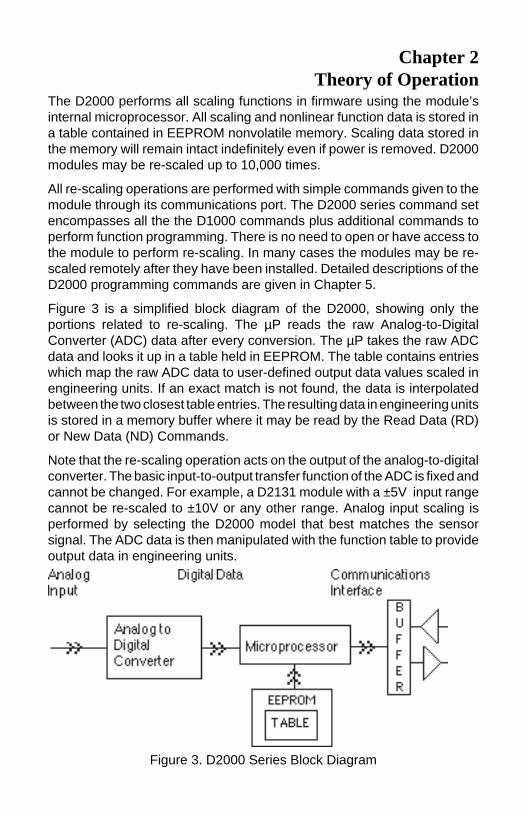
Figure 3 is a simplified block diagram of the D2000, showing only theportions related to re-scaling. The µP reads the raw Analog-to-DigitalConverter (ADC) data after every conversion. The µP takes the raw ADCdata and looks it up in a table held in EEPROM. The table contains entrieswhich map the raw ADC data to user-defined output data values scaled inengineering units. If an exact match is not found, the data is interpolatedbetween the two closest table entries. The resulting data in engineering unitsis stored in a memory buffer where it may be read by the Read Data (RD)or New Data (ND) Commands.

Note that the re-scaling operation acts on the output of the analog-to-digitalconverter. The basic input-to-output transfer function of the ADC is fixed andcannot be changed. For example, a D2131 module with a ±5V input rangecannot be re-scaled to ±10V or any other range. Analog input scaling isperformed by selecting the D2000 model that best matches the sensorsignal. The ADC data is then manipulated with the function table to provideoutput data in engineering units.

Chapter 2Theory of Operation

Figure 3. D2000 Series Block Diagram

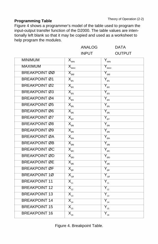
Theory of Operation (2-2)Programming TableFigure 4 shows a programmer’s model of the table used to program theinput-output transfer function of the D2000. The table values are inten-tionally left blank so that it may be copied and used as a worksheet tohelp program the modules.

ANALOG DATA

INPUT OUTPUT

MINIMUM XMIN YMIN

MAXIMUM XMAX YMAX

BREAKPOINT ØØ XØØ YØØ

BREAKPOINT Ø1 XØ1 YØ1









BREAKPOINT ØA XØA YØA

BREAKPOINT ØB XØB YØB

BREAKPOINT ØC XØC YØC

BREAKPOINT ØD XØD YØD

BREAKPOINT ØE XØE YØE

BREAKPOINT ØF XØF YØF

BREAKPOINT 1Ø X1Ø Y1Ø

BREAKPOINT 11 X11 Y11






Figure 4. Breakpoint Table.

Theory of Operation (2-3)The two most important points in the table are the Minimum and Maximumpoints. These two table entries specify the minimum and maximum end-points of the transfer function curve. For instance, a D2121 has a range of±1V, and the standard table values are:

Analog Input Data Output

Minimum -1V -01000.00Maximum +1V +01000.00

Plotted on a graph (Figure 5), these two points specify the endpoints of thetransfer curve. In this case, the analog input variable X is in terms of voltage.The X values in the table specify the minimum and maximum voltages thatmay be applied to the analog input that will result in a linearized output. (TheX voltage values are actually stored in memory in terms of ADC binary data).Voltage values applied to the analog input that are more negative than Xminwill result in an overload output of -99999.99. Similarly, voltage valuesgreater than Xmax will result in +99999.99.

Figure 5. Function Endpoints

The corresponding Y values in the table specify the output data of theminimum and maximum points. In this case, a -1V input corresponds to anoutput of -01000.00mV. The Y values are always stored in the standard dataformat of sign, 5 digits, decimal point and two additional digits.

The minimum and maximum points are the only table values necessary tospecify a linear transfer function. For analog input values between Xmin andXmax, the output values are determined by linearly interpolating betweenthe minimum and maximum points. For instance, in the case of the D2121,

Theory of Operation (2-4)an analog input value of +.5V is linearly interpolated to an output value of+00500.00 (Figure 5).

It should be apparent at this point that a D2000 module may be re-scaled bymodifying the minimum and maximum values in the table. This may beaccomplished by using the Minimum (MN) command and the Maximum(MX) command. Using the D2121 ±1 volt module as an example, we mayuse the MN and MX commands to alter the table to look like this:


Minimum 0V +00100.00Maximum +1V +00800.00

In this case the minimum point is 0V, corresponding to the output data+00100.00. The maximum point is +1V input and +00800.00 output. Thegraph of this equation is shown in Figure 6.

By changing the minimum and maximum values in the table, an infinite

Figure 6

number of linear functions may be specified, bounded by X values of ±1Vand Y values of ±99999.99. Figure 7 shows a few possibilities.

The exact procedure necessary to program the maximum and minimumpoints is described in Chapter 5.

Theory of Operation (2-5)

BreakpointsFrom Figure 4, we can see that most of the transfer function table is reservedfor “Breakpoints”. Breakpoints are used to modify the basic linear curvedefined by the Minimum and Maximum points to create nonlinear functions.

Nonlinear functions in the D2000 are approximated by using linear seg-ments which are specified by the data values held in the Breakpoint Table.Up to 23 breakpoints may be programmed to specify up to 24 linearsegments. Figure 8 illustrates the action of the breakpoints. Figure 8a showsa basic linear transfer function described by the Minimum and Maximumpoints. Figure 8b shows the effect of one breakpoint used to modify the linearfunction. Notice that the breakpoint has created a nonlinear functiondescribed by two linear segments joined at the breakpoint. Figure 8c showsthat two breakpoints may be used to specify a nonlinear curve described bythree linear segments. Up to 23 breakpoints may be used to create complexnonlinear curves.

Figure 7. Examples of Linear Functions.

a b cFigure 8. Breakpoint Examples

Theory of Operation (2-6)Breakpoints are stored in the EEPROM table in the same fashion as theminimum and maximum points. Each breakpoint is described by an X-Y pairspecifying the analog input value at which the breakpoint occurs and thecorresponding output data value. When the microprocessor reads theanalog (X) data from the ADC, it searches the breakpoint table to find the Xvalue closest to the input data. The micro then linearly interpolates betweentwo breakpoints to calculate the resulting output data.

Any number of breakpoints up to 23 values may be specified. The breakpointtable must be filled progressively starting with Breakpoint 00 to Breakpoint16 (hex). Unused or “erased” breakpoints are not used in the functioncalculation.

Let’s use the D2121 ±1V module again as an illustrative example to showthe effect of a breakpoint. Figure 9 shows the D2121 function table with 1breakpoint programmed:

Analog Input Data OutputMinimum -1V -01000.00Maximum +1V +01000.00Breakpoint 00 +0.2V +00800.00Breakpoint 01 - - - - - - - - - - - - -…………………………

Breakpoints 01 through 16 (hex) are erased and do not enter the functioncalculation. The Minimum and Maximum table entries contain the standarddata values of ±01000.00mV. The new curve is shown in Figure 9.

Figure 9

Theory of Operation (2-7)Notice how the breakpoint has affected the whole curve, creating a nonlinearfunction. Here are a few samples of the input-output values that may beobtained from this curve:

Analog Input Data Output-.8V -00700.00-.6V -00400.00-.4V -00100.00-.2V +00200.000V +00500.00+.2V +00800.00+.4V +00850.00+.6V +00900.00+.8V +00950.00

The procedure to create a breakpoint table is detailed in Chapter 4.

D2000 COMMAND SET

The D2000 module series incorporates the same command set as theD1000 series, with new commands added to facilitate custom rangeprogramming. The added D2000 commands are used only for program-ming. For normal operational commands, refer to the D1000 manual.

CAUTION: THE D2000 PROGRAMMING COMMANDS MUST BE USEDWITH CARE. EACH OF THE COMMANDS IS CAPABLE OF DESTROY-ING FACTORY CALIBRATION.

All of the commands added to the D2000 series are write-protected to guardagainst accidentally altering data values stored in the module’s EEPROM.Therefore, all programming commands must be preceded with a WriteEnable (WE) command.

All of the D1000 command-response protocol rules apply to the D2000.

This section is intended only to describe the new commands. For program-ming information refer to Chapter 5.

BREAK POINT (BP)Nonlinear functions may be approximated in the D2000 by describing thefunction curve with a series of line segments (see Figure 1). The linesegments are programmed into the D2000 using the BreakPoint (BP)command. A breakpoint specifies the intersection between two linearsegments used to approximate the nonlinear transfer function. Up to 23breakpoints may be used to specify 24 linear segments in a curve.

To program a breakpoint, a known analog stimulus must be applied to thesensor input of the D2000 module. This specifies the input variable (X-axis)location of the breakpoint. The corresponding output data (Y-axis) of thebreakpoint is specified as an argument to the BreakPoint (BP) command.

Example: (Spaces have been added to the command for clarity)

Command: $1 BP 03 +00100.00Response: *

Command: #1 BP 03 +00100.00Response: *1BP 03 +00100.00FA (FA = checksum)

The first two characters following the “BP” command specify the breakpointnumber. Up to 23 breakpoints may be programmed into the D2000. In thesample command above, breakpoint number “03” is being specified. Break-point numbers are expressed in two-digit hexadecimal notation, rangingfrom “00” to “16” for a total of 23 (decimal) points. During a normal

Chapter 3Command Set

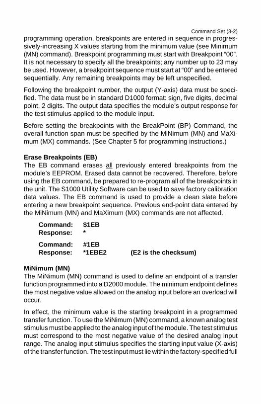
Command Set (3-2)programming operation, breakpoints are entered in sequence in progres-sively-increasing X values starting from the minimum value (see Minimum(MN) command). Breakpoint programming must start with Breakpoint “00”.It is not necessary to specify all the breakpoints; any number up to 23 maybe used. However, a breakpoint sequence must start at “00” and be enteredsequentially. Any remaining breakpoints may be left unspecified.

Following the breakpoint number, the output (Y-axis) data must be speci-fied. The data must be in standard D1000 format: sign, five digits, decimalpoint, 2 digits. The output data specifies the module’s output response forthe test stimulus applied to the module input.

Before setting the breakpoints with the BreakPoint (BP) Command, theoverall function span must be specified by the MiNimum (MN) and MaXi-mum (MX) commands. (See Chapter 5 for programming instructions.)

Erase Breakpoints (EB)The EB command erases all previously entered breakpoints from themodule’s EEPROM. Erased data cannot be recovered. Therefore, beforeusing the EB command, be prepared to re-program all of the breakpoints inthe unit. The S1000 Utility Software can be used to save factory calibrationdata values. The EB command is used to provide a clean slate beforeentering a new breakpoint sequence. Previous end-point data entered bythe MiNimum (MN) and MaXimum (MX) commands are not affected.

Command: $1EBResponse: *

Command: #1EBResponse: *1EBE2 (E2 is the checksum)

MiNimum (MN)The MiNimum (MN) command is used to define an endpoint of a transferfunction programmed into a D2000 module. The minimum endpoint definesthe most negative value allowed on the analog input before an overload willoccur.

In effect, the minimum value is the starting breakpoint in a programmedtransfer function. To use the MiNimum (MN) command, a known analog teststimulus must be applied to the analog input of the module. The test stimulusmust correspond to the most negative value of the desired analog inputrange. The analog input stimulus specifies the starting input value (X-axis)of the transfer function. The test input must lie within the factory-specified full

Command Set (3-3)scale input range of the module.

The argument of the MN command specifies the starting output value (Y-axis) of the transfer function.

Command: $1MN -00100.00Response: *

Command: #1MN -00100.00Response: *1MN-00100.00A2 (A2 is the checksum)

MaXimum (MX)The MaXimum (MX) command specifies the most positive analog inputallowed before an overload indication will occur. The MaXimum commandalso defines the positive end point of a transfer function programmed into theSCM9B-2000. To perform a MaXimum command, a known analog stimulusmust be applied to the sensor input of the SCM9B-2000 unit. This test inputmust correspond to most positive value of the programmed transfer func-tion. The analog test signal must remain within the factory-specified inputrange of the SCM9B-2000 module. The analog input establishes themaximum input value (X-axis) for the transfer function. The maximum outputvalue (Y-axis) is specified as the argument of the MaXimum command.

Command: $1MX +00500.00Response: *

Command: #1MX +0500.00Response: *1MX+00500.00AE (AE is the checksum)

Command Set (3-4)

This section will cover the mechanics of programming a custom transferfunction into the D2000. All programming is performed through the commu-nications port of the D2000 using a dumb terminal or a computer operatingas a dumb terminal. In field installations where AC power is not readilyavailable, programming may be accomplished with standard battery-oper-ated ASCII terminals. Since all programming is accomplished through thecommunications port, access to the module is not necessary and rangingmay be accomplished remotely.

Programming SoftwareAlthough all programming functions may be accomplished with a dumbterminal, the task may be greatly simplified with the use of utility softwarerunning on a computer. S1000 utility software is provided free of charge andwill run on many of the popular personal computers. The software providesmany enhancements that are not available through manual programming.In many applications the D2000 modules may be programmed strictlythrough software methods without the need for external excitation sources.

GENERAL GUIDELINES

Input ScalingThe full scale analog input characteristics of a D2000 module may not bealtered by the user. Input scaling is accomplished by selecting the correctD2000 model for the application. Programming a D2000 involves alteringthe scaling of the unit’s A/D converter output. There is no provision forchanging the gain or offset of the analog circuitry.

ExcitationWhen the D2000 modules are programmed manually with a terminal,external excitation sources are necessary to establish calibration pointswithin the module. Excitation may be provided by standard voltage, currentand frequency calibration sources. The final absolute accuracy of themodule is directly dependent on the accuracy of the excitation sources. Insome cases, the excitation may be generated directly by the system beingmonitored. In situations when excitation sources are not available orimpractical, modules may be programmed with S2000 programming soft-ware without excitation.

Chapter 4Programming

Programming (4-2)

Output Data FormatOne of the preliminary decisions to be made before programming is how theoutput data will be structured. All D1000/2000 sensor modules communi-cate data in a fixed format of sign, five digits, decimal point, and twoadditional digits; +00100.00 is an example. The fixed format is used tosimplify software in host computers. Despite the fixed format, the program-mer has a certain amount of flexibility to structure the output data for the bestcompromise between resolution and readability. For example, an outputindication of +.05 volts could be structured in three different output formats:

+00000.05 (+.05 volts)+00050.00 (+50 millivolts)+50000.00 (50,000 microvolts)

The first consideration must be the resolution or the number of output countsavailable in the output structure. If the overall function span is 0 to +50millivolts, the first example would only yield 5 counts from +00000.00 to+00000.05. In most applications this resolution would not be acceptable.The next obvious output structure is to output the data in units of millivolts,as shown in the second example. This format would give us 5,000 countsof resolution. Finally, the third example expresses the output data in units ofmicrovolts to give a possible resolution of five million counts.

The second factor that must be considered is the performance limitations ofthe A/D converter. The best resolution of the ADC is 32,768 counts.Resolution is degraded by round-off errors, noise, etc., so that a practicalexpectation for usable resolution would be in the range of 5,000 to 20,000counts. Output resolution may be limited by picking a suitable output formator by using the appropriate ‘displayed digits’ setup as described in theD1000 Setup section.

In the present example of the 0 to 50mV output, probably the bestcompromise is to use the millivolt form to represent the data. This gives5,000 count resolution in easy to interpret units of millivolts. In this case the‘displayed digits’ setup should be programmed to display all digits.

It may be tempting to use the microvolt output format in an effort to extractthe maximum counts of resolution, but the units digit will tend to be noisy.The uncertainty of the units digit may be counteracted somewhat by usinglarge amounts of digital filtering in the module setup. In this case the setupdata should specify a ‘displayed digits’ setting of the first five digits only,since the digits to the right of the decimal point have no meaning. Also, themicrovolt format is a bit more awkward to interpret than the millivolt format.

In some cases it may require a bit of creative thinking to develop a suitableoutput format. For example, a D2000 module may be required to output data

Programming (4-3)

in units of specific gravity. In a typical application, the specific gravity outputmay range between .5 and 2. The most obvious output format would havethe output data ranging from +00000.50 to +00002.00. This format givesonly 150 counts of resolution between the minimum and maximum outputs.However, since the specific gravity of water is defined to be 1, the output maybe scaled in units of “percent of water”. The specific gravity of water wouldthen be 100 percent. The output data in ‘percent’ units would range from+00050.00 to +00200.00. This format allows up to 15,000 counts ofresolution and reads out in units that may be easily interpreted.

LinearityThe analog-to-digital converter used in the D2000 has a typical integralnonlinearity of .1% of full scale. At the factory the ADC linearity is correctedby using breakpoints to reduce the nonlinearity to .01%. If the breakpointtable is erased with the Erase Breakpoints (EB) command, the linearitycorrection is lost. In some cases when linear re-scaling is performed, theprogrammer may take advantage of the factory linearity correction (Ex-ample L-4). If less than the full analog input scale is used, the linearitycorrection should be erased with the EB command. Linearity may beimproved with the use of new breakpoints (Example N-5).

SCM9B-2000 Function ProgrammingThe D2000 transfer function may be programmed by modifying the functiontable with the MiNimum (MN), MaXimum (MX) and BreakPoint (BP) com-mands. All three commands operate on the same basic principle. Eachcommand is used to specify an input-output (X,Y) data pair in the functiontable. To perform a programming command, a known analog excitationmust be applied to the analog input of the D2000 module. The excitation maybe a voltage, current, frequency, or the output of a resistive bridge,depending on the specific D2000 module type. The known excitation valueis used to create the “X” values in the function table. The “Y” table values areloaded with data specified in the command argument.

For example, suppose we have a D2121 ±1V module and we’d like toprogram the minimum table value to Xmin = -.5V, Ymin = -00100.00. Apply-.5 volts to the module input with a calibrated voltage source. Perform theMiNimum (MN) command with the Ymin value as the data argument in theMN command:

Command: $1WE (MN is write-protected)Response: *

Command: $1MN-00100.00Response: *

Programming (4-4)

When the module executes the MN command, the microprocessor performstwo functions. First, it reads the data produced by the A/D converter with the-.5V input. The A/D converter data is stored as Xmin in the function table.The micro then reads the argument of the MN instruction, which in this caseis -00100.00, and stores this value in the table as Ymin. This completes thedefinition of the new minimum point. The module will immediately use thisnew minimum point data in calculating output data.

Note that the MN command will write over any previous data in the table. Theold data is permanently lost. This is also true with the MaXimum (MX) andBreakPoint (BP) commands. Since the MN, MX, and BP commands affectthe calibration of the module, they must not be used indiscriminately unlessyou are prepared to re-calibrate the unit.

Linear ScalingRescaling the D2000 to a linear transfer function is the easiest and mostcommon way to reprogram the module. The linear scale function is definedby specifying the two endpoints of the linear function (see Figure 7). Anylinear function within the analog input range of the module may be defined.

Custom scaling requires a calibrated analog input signal to define the endpoints of the linear transfer function. The signal could be a voltage, current,or frequency depending on the specific model type. The MiNimum andMaXimum commands are used to program the end point data into themodules’s memory.

Programming procedures:

1. Make sure the module has not been previously programmed with BreakPoint (BP) Commands. If it has, clear the breakpoints with the EraseBreakpoints (EB) command.

2. Clear any data in the output offset register with the Clear Zero (CZ)command.

3. Determine the endpoints which will be used to define the linear function.The analog input values must lie within the full scale operating range of themodule. The analog inputs used to determine the endpoints will also definethe display overload outputs of the module. Construct an output data formatthat is best suited for your application.

4. Apply a calibrated analog signal to the module input corresponding to themost negative input of the desired linear scale. Perform a Minimum (MN)command to store the function endpoint into the modules’s memory.

5. Apply a calibrated analog signal to the module input corresponding to the

Programming (4-5)

most positive analog input value. Perform a Maximum (MX) command toload the endpoint data into the module memory.

6. Verify that the transfer function has been correctly loaded into the moduleby applying test inputs to the module and reading out the data with the ReadData (RD) command.

Example L-1Reprogram a D2251, 4-20mA module to output data in terms of percent; thatis, 4mA will read out to be 0% and 20mA will read out as 100%.

1. If the module had been previously programmed with breakpoints, erasethe function table with the Erase Breakpoints (EB) command:

Command: $1WEResponse: *


2. Clear any offset data with the Clear Zero command:


Command: $1CZResponse: *

3. The minimum analog input in this case is 4mA. Any current less than 4mAwill result in a negative over-range (-99999.99). The maximum positive inputis 20mA. Since the minimum value of 4mA corresponds to 0%, theappropriate output data would be +00000.00. The output data correspond-ing to 20mA is +00100.00. This data format gives us whole units of “percent”to the left of the decimal point. To get the maximum resolution from themodule, set up the number of displayed digits with the SetUp (SU) so thatall digits are displayed.


Command: $1SU310701C2 (typical)Response: *

Programming (4-6)

4. Apply exactly 4mA to the current input of the module. Program theendpoint with the MiNimum command:


Command: $1MN+00000.00Response: *

5. Apply exactly 20mA to the module input and store the maximum endpointwith the MaXimum (MX) command:


Command: $1MX+00100.00Response: *

6. Verify the module response by testing it with various inputs within itsrange:

Input Current Output Data

8mA +00025.0012mA +00050.0016mA +00075.00

Rescaling is now complete.

Example L-2A paddle-wheel flow sensor will be used to monitor the flow of water in a pipe.The characteristics of the sensor and the size of the pipe results in an outputfrequency of 10 Hz per gallon per minute. The operating range is from 1 to20 gallons per minute.

We would like to scale a D2000 module to output data in units of .1 gallons.

The logical module choice in this application is the D2601 frequency inputmodule. The frequency output of the flow sensor will range from 10 Hz to 200Hz, easily within the 5 Hz to 20 kHz range of the D2601.

1. Erase Breakpoints:



2. Clear Zero:

Programming (4-7)



3. The minimum endpoint in this case is 10 Hz corresponding to an outputof +00001.00 gpm. The maximum frequency at 20 gpm is 200 Hz. Themaximum output data is +00020.00. To get .1 gpm resolution, set up themodule to display six digits:


Command: $1SU31070182 (typical)Response: *

4. Using a calibrated frequency generator, apply 10 Hz to the module input.Set the minimum point:



5.Set the frequency generator to 200 Hz to program the maximum point:



6. Use the frequency generator to verify a few points in the scale:


30 Hz +00003.00100 Hz +00010.00155 Hz +00015.50

Programming is now complete and the D2601 can be attached to the flowsensor.

Programming (4-8)

Example L-3In many cases the analog calibration values may be produced directly by thesensors to be used in a system. The module may be re-ranged in the fieldto encompass any errors due to sensor inaccuracies.

In this example, we wish to use a pressure sensor to measure the volumeof water in a cylindrical tank that is 10 feet tall with the capacity of 1500gallons. The pressure sensor is mounted at the bottom of the tank so thatit will produce an output corresponding to the height of water in the tank. Thepressure sensor chosen produces 1V @ 0 psi and 5V @ 10 psi. A full tankwith 10 feet of water will produce 4.335 psi (1 ft = .4335 psi), well within therange of the pressure sensor. A D2131 ±5V input module will be used as theinterface.

1. Erase Breakpoints:



2. Clear Zero:



3. To produce the analog Xmin and Xmax endpoint values, we will use theactual water levels in the tank to produce a calibration pressure. Theaccuracy of the pressure transducer is not important, as long as it is stableand linear. To set the minimum value, we will empty the tank and set theminimum value to +00000.00. The maximum value will be programmed withthe tank full and the maximum output data will be set to +01500.00 gallons.In this case an output resolution in units of gallons is acceptable and we canset up the module so that 5 digits are displayed. The digits to the right of thedecimal point will always read out “00”.



Programming (4-9)

4. With the tank empty, program the minimum point:



5. Fill the tank with water and program the maximum point:



6. Verify the scaling. In this case, it is difficult to verify the scaling quickly andaccurately. A “ballpark” check can be made by letting water out of the fulltank and checking to see if the module output readings are “reasonable”. Amore accurate check can be made by filling the tank with known amountsof water and verifying the output readings.

Example L- 4A SCM9B-2251 4-20mA module will be used to provide a computerinterface to an existing process 4-20mA signal. The loop transmitterproduces a linear 4-20mA signal corresponding to a sensor temperature of0-200 degrees C. In this case we’d like to take advantage of the factorylinearity correction in the SCM9B-2251 for greater accuracy. To do this, wemust use the same analog input minimum and maximum points as pro-grammed at the factory. The SCM9B-2251 minimum and maximum pointsare 0mA and 25mA. The 4-20mA span of the process transmitter must beextrapolated to 0-25mA to provide the correct data when using the MN andMX commands. The transfer relationship of the 4-20mA transmitter can bedescribed by the equation:

T = 12.5 X mA - 50

Plug values of 0mA and 25mA into the equation to derive extrapolatedvalues of T:

T = 12.5 X (0) - 50 = - 50

T = 12.5 X (25) - 50 = + 262.5

These values will be used in the MN and MX instructions.

Program the module:

1. In this case it is assumed that the SCM9B-2251 is fresh from the factoryand it still contains linearity correction in the breakpoint table. In order to takeadvantage of the linearity correction, the breakpoints will not be erased.

Programming (4-10)

2. Clear zero:



3. The minimum endpoint has been extrapolated to be -00050.00 @ 0mA.The maximum point is +00262.50 @ 25mA. We’ll setup the module todisplay temperature with .1 degree resolution:



4. Apply 0mA (open circuit) to the current input and program the minimumpoint:


Command: $1MN-00050.00Response: *

5. Apply exactly 25mA to the current input to program the maximum point:



6. Apply test currents to the module to verify the scaling:

Apply 4mA to the input:

Command: $1Response: *+00000.00

Apply 20mA to the input:


Nonlinear functions may be created by first specifying a linear function withthe MiNimum (MN) and MaXimum (MX) commands. The linear function isthen modified by using the BreakPoint (BP) command. Almost any practicalnonlinear function may be approximated provided it satisfies two rules:

1) The nonlinear function must be totally enclosed by the rectangular areadefined by the minimum an maximum points. Figure 10 gives examples ofthe “rectangular area”.

Figure 10. Example of "Rectangular Area".

Figure 11 illustrates a function that is not possible since a portion of the curvelies outside of the rectangle. In most cases this limitation may be overcomeby simply re-arranging the curve so that the rectangular area is larger. Figure12 shows the same curve as Figure 11, but slightly modified to allow it to beprogrammed into the D2000.

Figure 11. Illegal Function.

Figure 12 Modified Function.

Chapter 5Nonlinear Programming

Nonlinear Programming (5-2)

2) The nonlinear function must be a single-valued function of X. That is, foreach input value, there can exist only one output value. Figure 13 shows twoillegal functions. This limitation is seldom encountered in natural phenome-non.

Figure 13. Examples of Illegal Functions.

Programming Steps1) Define the function data points to be programmed2) Erase breakpoints3) Clear zero4) Use SetUp (SU) command to set number of displayed digits5) Program the minimum endpoint6) Program the maximum endpoint7) Program breakpoints8) Verify the function

Step 1. Define the function data points to be programmed. The ability of theD2000 to simulate a nonlinear transfer function is highly dependent on thelocation of the breakpoints selected by the programmer. The ultimateconformity to the desired function is directly dependent on the linear-segment approximation loaded into the module. The D2000 gives theprogrammer a great deal of flexibility in how the breakpoints are placed. Inareas where the function curves sharply, or where greater accuracy isdesired, breakpoints may be placed close together for better conformity tothe desired function. The chart in Figure 4 is a handy form to help organizethe breakpoint data.


Step 2. The existing breakpoint table should be cleared by using the EraseBreakpoints (EB) command. This command will completely erase thebreakpoint table. Any previous breakpoint information will be permanentlylost.

Command: $1WEResponse : *


Step 3. Clear any data stored in the output offset register by using the ClearZero (CZ) command:



Step 4. Use the SetUp (SU) command to program the correct number ofdisplayed digits:



Step 5. Start the function programming by setting the minimum point usingthe MiNimum (MN) command as described in the linear scaling section.

Step 6. Set the maximum function point with the MaXimum command asdescribed in the linear scaling section.

Step 7. Use the BreakPoint (BP) command to program the nonlinearfunction into memory. Apply the proper excitation to the module for Break-point 00. Use the BreakPoint command to enter the data into memory:


Command: $1BP00+00100.00Response: *


It may be useful to verify that the breakpoint data has indeed been recordedin memory. Without changing the excitation, read the output data:


The output data should match the data programmed with the Breakpointcommand.

Once Breakpoint 00 has been entered, proceed to Breakpoint 01. Set theanalog excitation for the correct value for Breakpoint 01. Load the breakpointinto memory using the BreakPoint command. Be sure to specify ‘01’ in theBreakPoint command:



Verify that the data has been entered properly:

Command: $1Response: +00200.00

Continue this process until all breakpoints have been programmed.

Step 8. Test the input-output transfer function of the module to verify that thebreakpoint data has been entered properly. Large errors in the output dataare generally caused by improper breakpoint programming. In most casesit is not necessary to repeat the whole breakpoint sequence if the error isconfined to one portion of the curve. Breakpoints may be re-programmedindividually to correct any errors. However, it is not possible to insert newbreakpoints in between existing points of the table to correct for a poor initialfunction approximation.

Example N–1A voltage-output pressure sensor produces 0V @ 100 psi and 5V @ 600 psi.Its output characteristic is nonlinear and may be described by the equation:

P = 100 + 80 V + 4 V2

where

V = sensor output in voltsP = pressure in psi

A simple linear equation may be derived by using the endpoint data:P = 100 + 100V


Unfortunately, describing the sensor output with this equation results in a 25psi error at V = 2.5V.

To obtain better accuracy, we may approximate the quadratic transferfunction using breakpoints. Since the sensor output range is 0–5V, theD2131 with an input range of ±5V is most suitable for this application. Forsimplicity, we will use only four evenly-spaced breakpoints to plot thefunction. This will result in a function approximation with a maximum errorof 1 psi. For better conformity, more breakpoints may be used.

1. First, construct the function table:

Analog Input Output

Minimum 0V +00100.00Maximum 5V +00600.00Breakpoint 00 1V +00184.00Breakpoint 01 2V +00276.00Breakpoint 02 3V +00376.00Breakpoint 03 4V +00484.00

Notice that we’ve broken up the curve into five evenly-spaced voltagesegments by using four breakpoints. The breakpoint output values wereobtained by plugging the breakpoint voltage values into the quadraticequation that describes the sensor.

2. Prepare the D2131 by erasing any stored breakpoints: (All programmingcommands must be preceded by a Write Enable (WE) command. In theinterest of simplicity, the Write Enable commands are not shown in this orany of the following examples.)


3) Clear any data in the output offset register:


4) We will setup the output data to display psi with .1 resolution:


(The SU data may vary depending on your particular module setup. See theSetup section in the D1000 manual.)


5. Apply 0 volts (short) to the input of the D2131 to enter the minimum pointof 100 psi:


6. To set the maximum point, apply 5V to the input and program themaximum point to be 600 psi:


7. Program the first breakpoint:

Apply 1 volt to the input and perform the BreakPoint command:


Verify the breakpoint data:


Repeat the procedure for the remaining breakpoints:

Apply 2 volts to the input:









The function programming is now complete.


8. The transfer function may be verified by applying test inputs to the moduleand obtaining output data. The data can then be compared to the originalquadratic equation to check for conformity error.

Example:

Apply .5 volts to the D2131 input and read data:


To check, plug .5 volts into the quadratic equation:

P = 100 + 80 (.5) + 4 (.5)2 = 141

The conformity error at this point is +1 psi.

Example N–2A pressure sensor rated for 0-200 psi has a nonlinear transfer functiondescribed by the relationship:

V = 4 x 10-3 P + 5 x 10-6 P2

V = 0 to 1 voltsP = 0 to 200 psi

Use a D2121 ±1V input module to linearize the sensor output and convertthe data to engineering units.

This example differs from Example N–1 because the desired output data inpsi is the independent variable in the equation. One solution to this problemwould be to convert the equation to a form of P = f (V) and then proceed aswe did in Example N–1. However, this kind of mathematical rigor is notnecessary. To program the D2121, we simply need to construct a table ofX,Y pairs. In this case, we may choose breakpoints to be in even intervalsof psi, and then calculate the matching values of V. Our table with fourbreakpoints would look like this:

Input Output

Minimum 0V +00000.00Maximum +1V +00200.00Breakpoint 00 .168V +00040.00Breakpoint 01 .352V +00080.00Breakpoint 02 .552V +00120.00Breakpoint 03 .768V +00160.00

Notice that in this case, the breakpoints were selected by picking evenintervals of pressure. The pressure values are then plugged into the sensor


equation to produce the breakpoint voltages. The mechanics of entering thebreakpoints is the same as in Example 1.

If better conformity is required, more breakpoints may be used. However,breakpoints cannot be simply added to the table at random. Breakpointsmust be entered in sequence starting at the minimum value and progress inever-increasing values of the X variable. To obtain better conformity, a newfunction table must be started from the beginning. Therefore, to avoidneedless trial and error, it is best to test the breakpoint table on paper todetermine if the conformity error is acceptable. Another approach is tosimply use all 23 breakpoints available for the best conformity.

For this example, we may improve the conformity error by using ninebreakpoints:

Input OutputMinimum 0V +00000.00Maximum 1V +00200.00Breakpoint 00 .082V +00020.00Breakpoint 01 .168V +00040.00Breakpoint 02 .258V +00060.00Breakpoint 03 .352V +00080.00Breakpoint 04 .450V +00100.00Breakpoint 05 .552V +00120.00Breakpoint 06 .658V +00140.00Breakpoint 07 .768V +00160.00Breakpoint 08 .882V +00180.00

Example N–3In many cases, the system transfer function may not be known. In thesesituations, a D2000 may be programmed empirically using test inputsderived by the system itself.

A standpipe in a municipal water system has an irregular shape, as shownin Figure 14. It is desirable to obtain a direct reading of the volume of watercontained in the standpipe. Because of the shape, a simple water heightmeasurement would give grossly inaccurate readings of volume. Also, theactual relationship of volume to height is complex and unknown.

The standpipe is 50 feet tall and has a known capacity of 30,000 gallons. Apressure sensor may be used at the base of the standpipe to obtain areading of the water height. Since 1 foot of water produces a pressure of.4335 psi, the maximum pressure expected is 50 X .4335 = 21.7 psi. Thepressure sensor we will use produces 0–5 volts for pressures of 0–25 psi.A D2131 ±5V input module will be used as the interface.


Install the pressure sensor and the D2131 in place at the standpipe. Preparethe D2131 by erasing breakpoints and clearing zero as detailed in ExampleN–1. In this case we will setup the D2131 to display four digits which willresult in an output resolution of 10 gallons.

Start programming with the standpipe empty. Enter the minimum value:


In this example, the maximum point may be programmed by filling thestandpipe to obtain the maximum pressure output. However, this is awk-ward and unnecessary. Since the standpipe capacity is known to be 30,000gallons and the pressure can never reach 25 psi, we can simulate amaximum that we know can never be attained. To do this we may apply 5Vto the module input to simulate 25 psi. The 5V source does not have to beaccurate. We can set the maximum value to 35,000 gallons, which is morethan the standpipe can hold.

Disconnect the pressure sensor and apply 5V to the module input:


Re-connect the pressure sensor to the D2131. Starting with the standpipeempty, we may begin to program the breakpoints. We will set a breakpointevery 1500 gallons for a total of 20 breakpoints.

Figure 14. Scaling When Transfer Function is Unknown.


To set the first breakpoint, fill the standpipe with 1500 gallons of water. Sincewe will be using actual volumes of water to ‘calibrate’ the standpipe, theaccuracy at which we can measure 1500 gallons will greatly influence thefinal performance of the system.

With 1500 gallons in the standpipe used as the input excitation, program thefirst breakpoint:


Test:


Fill the standpipe with an additional 1500 gallons to program the secondbreakpoint. The standpipe now holds 3000 gallons:



Repeat these steps until the standpipe is full. For each step, fill the standpipewith an additional 1500 gallons and program the breakpoint with theaccumulated amount of water in the standpipe. When the breakpointprogramming is complete, the D2131 will give a very accurate indication ofthe volume of water in the standpipe directly in units of gallons.

In this example, the actual transfer function of the system is unknown.Instead, the function is plotted in the field by applying known inputs to thesystem. Note that the voltage produced by the pressure sensor does nothave to be known to program the D2131. However it is wise to record thevoltages produced by the sensor at each breakpoint. With this information,replacement D2131’s may be programmed with a voltage source to avoidrepeating the tank filling exercise.

Example N–4Program a D2141 ±10V input module to calculate the square root of the inputsignal from 0 to 10V. We’ll keep the units in terms of millivolts so that thesquare root of 10,000 millivolts (10V) is 100. To simplify this example, wewill create a function with nine breakpoints at even 1V intervals.


1. Construct the function table:

Analog input Data Output

Minimum 0V +00000.00Maximum 10V +00100.00Breakpoint 00 1V +00031.62Breakpoint 01 2V +00044.72Breakpoint 02 3V +00054.77Breakpoint 03 4V +00063.25Breakpoint 04 5V +00070.71Breakpoint 05 6V +00077.46Breakpoint 06 7V +00083.67Breakpoint 07 8V +00089.44Breakpoint 08 9V +00094.87

2. Erase breakpoints:


3. Clear zero:


4. Display all digits:

Command: $1SU310701C2 (typical)Response: *

5. Program minimum by applying 0V (short) to input:


6. Program maximum by applying exactly 10 volts to the input:


7. Program breakpoints:

Apply 1 volt to the input:





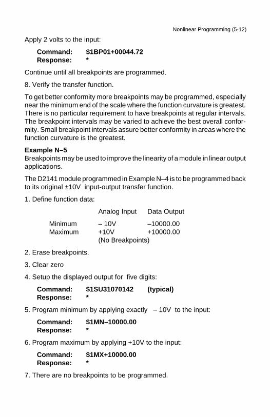
Continue until all breakpoints are programmed.

8. Verify the transfer function.

To get better conformity more breakpoints may be programmed, especiallynear the minimum end of the scale where the function curvature is greatest.There is no particular requirement to have breakpoints at regular intervals.The breakpoint intervals may be varied to achieve the best overall confor-mity. Small breakpoint intervals assure better conformity in areas where thefunction curvature is the greatest.

Example N–5Breakpoints may be used to improve the linearity of a module in linear outputapplications.

The D2141 module programmed in Example N–4 is to be programmed backto its original ±10V input-output transfer function.

1. Define function data:


Minimum – 10V –10000.00Maximum +10V +10000.00

(No Breakpoints)

2. Erase breakpoints.

3. Clear zero

4. Setup the displayed output for five digits:


5. Program minimum by applying exactly – 10V to the input:

Command: $1MN–10000.00Response: *

6. Program maximum by applying +10V to the input:


7. There are no breakpoints to be programmed.



– 5V –05010.000V –00020.00+ 5V +04990.00

During the verification process, we find that the module exhibits some errors.This is due to the .1% typical error inherent in the analog-to -digital converter.The nonlinearity may be corrected by using breakpoints. In this case,instead of using the breakpoints to create a nonlinear function, they will beused to ‘straighten’ the nonlinearity of the ADC. Only a few breakpoints arenecessary to reduce the linearity error to .02 % or less. In this case we willuse three breakpoints to linearize the module:


Minimum – 10V –10000.00Maximum + 10V +10000.00Breakpoint 00 – 5V –05000.00Breakpoint 01 0V +00000.00Breakpoint 02 +5V +05000.00

Since the minimum and maximum data have already been programmed,only Step 7 is necessary to program in the breakpoints.

After the breakpoints have been entered, verify the module transfer function:


– 7.5V –07502.000V +00000.00+7.5V +07498.00

This time the module output is in error by .02 % or less due to linearizingeffect of the breakpoints.

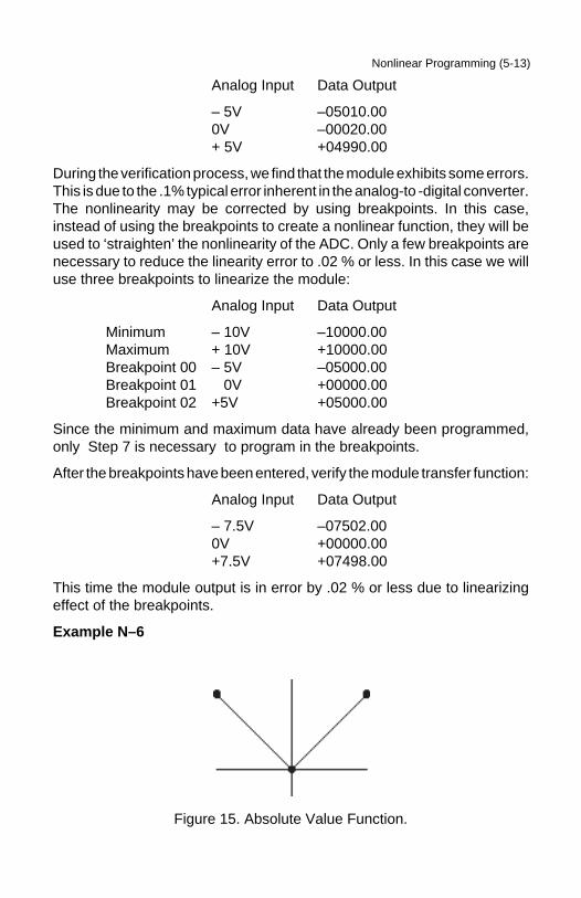
Example N–6

Figure 15. Absolute Value Function.


A D2141 module may be programmed to create an absolute-value functionas shown in Figure 15. However, this function violates the ‘rectangular area’rule. To overcome this limitation, the function may be re-drawn as shown inFigure 16. This curve satisfies the ‘rectangular area’ rule. The function tablefor this curve looks like this:


Minimum - 10V -00010.00Maximum +10V +10000.00Breakpoint 00 -9.990V +09990.00Breakpoint 01 0V +00000.00

The absolute-value function will be valid for inputs between - 9.990V and +10V. This technique may be used for other functions that violate the‘rectangular area’ rule.

Figure 16. Modified Absolute Value Function.

WARRANTY/DISCLAIMEROMEGA ENGINEERING, INC. warrants this unit to be free of defects in materials andworkmanship for a period of 13 months from date of purchase. OMEGA’s WARRANTY adds anadditional one (1) month grace period to the normal one (1) year product warranty to coverhandling and shipping time. This ensures that OMEGA’s customers receive maximumcoverage on each product.

If the unit malfunctions, it must be returned to the factory for evaluation. OMEGA’s CustomerService Department will issue an Authorized Return (AR) number immediately upon phone orwritten request. Upon examination by OMEGA, if the unit is found to be defective, it will berepaired or replaced at no charge. OMEGA’s WARRANTY does not apply to defects resultingfrom any action of the purchaser, including but not limited to mishandling, improper interfacing,operation outside of design limits, improper repair, or unauthorized modification. This WARRANTY is VOID if the unit shows evidence of having been tampered with or shows evidenceof having been damaged as a result of excessive corrosion; or current, heat, moisture or vibra-tion; improper specification; misapplication; misuse or other operating conditions outside ofOMEGA’s control. Components in which wear is not warranted, include but are not limited tocontact points, fuses, and triacs.

OMEGA is pleased to offer suggestions on the use of its various products. However, OMEGA neither assumes responsibility for any omissions or errors nor assumes liabilityfor any damages that result from the use of its products in accordance with informationprovided by OMEGA, either verbal or written. OMEGA warrants only that the parts manufactured by the company will be as specified and free of defects. OMEGA MAKESNO OTHER WARRANTIES OR REPRESENTATIONS OF ANY KIND WHATSOEVER,EXPRESSED OR IMPLIED, EXCEPT THAT OF TITLE, AND ALL IMPLIED WARRANTIESINCLUDING ANY WARRANTY OF MERCHANTABILITY AND FITNESS FOR A PARTICULARPURPOSE ARE HEREBY DISCLAIMED. LIMITATION OF LIABILITY: The remedies of pur-chaser set forth herein are exclusive, and the total liability of OMEGA with respect to thisorder, whether based on contract, warranty, negligence, indemnification, strict liability orotherwise, shall not exceed the purchase price of the component upon which liability isbased. In no event shall OMEGA be liable for consequential, incidental or special damages.

CONDITIONS: Equipment sold by OMEGA is not intended to be used, nor shall it be used: (1) asa “Basic Component” under 10 CFR 21 (NRC), used in or with any nuclear installation or activity;or (2) in medical applications or used on humans. Should any Product(s) be used in or with anynuclear installation or activity, medical application, used on humans, or misused in any way,OMEGA assumes no responsibility as set forth in our basic WARRANTY/DISCLAIMER language,and, additionally, purchaser will indemnify OMEGA and hold OMEGA harmless from any liabilityor damage whatsoever arising out of the use of the Product(s) in such a manner.

RETURN REQUESTS/INQUIRIESDirect all warranty and repair requests/inquiries to the OMEGA Customer Service Department.BEFORE RETURNING ANY PRODUCT(S) TO OMEGA, PURCHASER MUST OBTAIN ANAUTHORIZED RETURN (AR) NUMBER FROM OMEGA’S CUSTOMER SERVICE DEPARTMENT(IN ORDER TO AVOID PROCESSING DELAYS). The assigned AR number should then bemarked on the outside of the return package and on any correspondence.The purchaser is responsible for shipping charges, freight, insurance and proper packaging toprevent breakage in transit.

FOR WARRANTY RETURNS, please havethe following information available BEFORE contacting OMEGA:1. Purchase Order number under which

the product was PURCHASED,2. Model and serial number of the product

under warranty, and3. Repair instructions and/or specific

problems relative to the product.

FOR NON-WARRANTY REPAIRS, consultOMEGA for current repair charges. Have thefollowing information available BEFORE contacting OMEGA:1. Purchase Order number to cover the

COST of the repair,2. Model and serial number of the

product, and3. Repair instructions and/or specific problems

relative to the product.OMEGA’s policy is to make running changes, not model changes, whenever an improvement is possible. This affords our customers the latest in technology and engineering.OMEGA is a registered trademark of OMEGA ENGINEERING, INC.© Copyright 2005 OMEGA ENGINEERING, INC. All rights reserved. This document may not be copied, photocopied,reproduced, translated, or reduced to any electronic medium or machine-readable form, in whole or in part, withoutthe prior written consent of OMEGA ENGINEERING, INC.

Where Do I Find Everything I Need for Process Measurement and Control?

OMEGA…Of Course!Shop online at omega.com

TEMPERATURE�� Thermocouple, RTD & Thermistor Probes, Connectors, Panels & Assemblies�� Wire: Thermocouple, RTD & Thermistor�� Calibrators & Ice Point References�� Recorders, Controllers & Process Monitors�� Infrared Pyrometers

PRESSURE, STRAIN AND FORCE�� Transducers & Strain Gages�� Load Cells & Pressure Gages�� Displacement Transducers�� Instrumentation & Accessories

FLOW/LEVEL�� Rotameters, Gas Mass Flowmeters & Flow Computers�� Air Velocity Indicators�� Turbine/Paddlewheel Systems�� Totalizers & Batch Controllers

pH/CONDUCTIVITY�� pH Electrodes, Testers & Accessories�� Benchtop/Laboratory Meters�� Controllers, Calibrators, Simulators & Pumps�� Industrial pH & Conductivity Equipment

DATA ACQUISITION�� Data Acquisition & Engineering Software�� Communications-Based Acquisition Systems�� Plug-in Cards for Apple, IBM & Compatibles�� Datalogging Systems�� Recorders, Printers & Plotters

HEATERS�� Heating Cable�� Cartridge & Strip Heaters�� Immersion & Band Heaters�� Flexible Heaters�� Laboratory Heaters

ENVIRONMENTALMONITORING AND CONTROL�� Metering & Control Instrumentation�� Refractometers�� Pumps & Tubing�� Air, Soil & Water Monitors�� Industrial Water & Wastewater Treatment�� pH, Conductivity & Dissolved Oxygen Instruments M0661/0605

Documents

Digital Transmitters D2000 Series - OMEGA Engineering · Digital Transmitters MADE IN ... Tel: +31 (0)20 3472121 FAX: +31 (0)20 6434643 Toll Free in Benelux: 0800 0993344 ... 1000