DIMENSIONALITY REDUCTION:DIMENSIONALITY REDUCTION:DIMENSIONALITY REDUCTION:DIMENSIONALITY REDUCTION:DIMENSIONALITY REDUCTION:DIMENSIONALITY REDUCTION:DIMENSIONALITY REDUCTION:DIMENSIONALITY REDUCTION:

PCA, MDSPCA, MDSPCA, MDSPCA, MDS

Rita Osadchy

slides are due to L.Saul , A. Ng, and A. Ghodsi

Topics

� PCA� MDS� IsoMap� LLE� LLE� EigenMaps

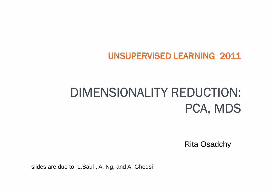
Types of Structure in High Dimension

� Clumps� Clustering� Density Estimation

� Low Dimensional Manifolds� Linear � NonLinear

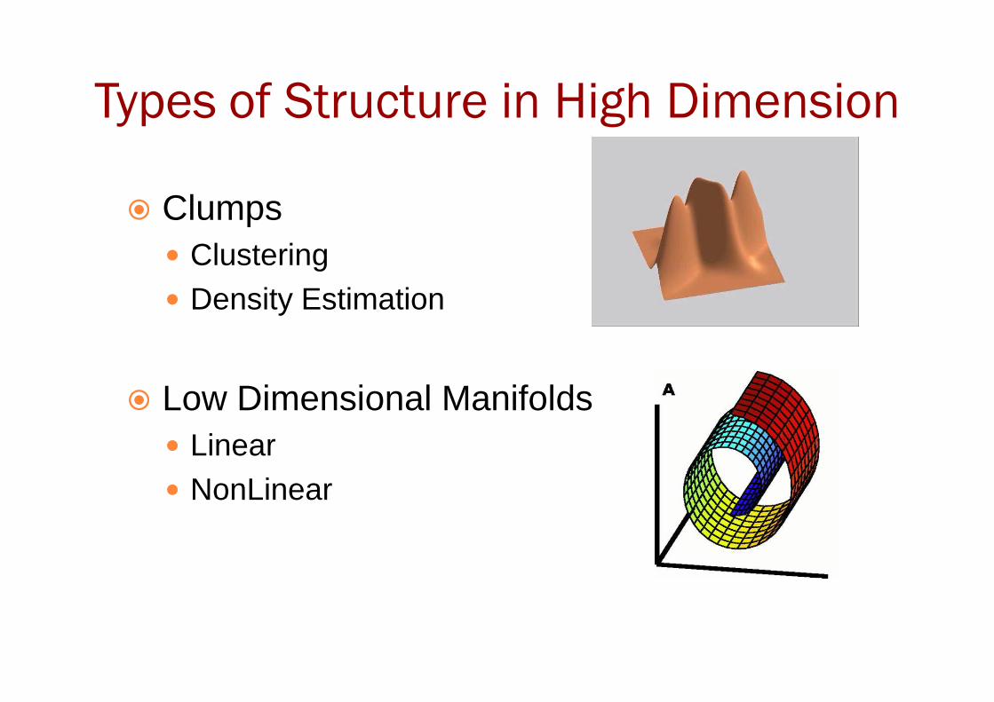
Dimensionality Reduction

� Data representationInputs are real-valued vectors in a high dimensional space.

� Linear structure� Linear structureDoes the data live in a low dimensional subspace?

� Nonlinear structureDoes the data live on a low dimensional submanifold?

Dimensionality Reduction

� QuestionHow can we detect low dimensional structure in high dimensional data?

� Applications� Applications� Digital image and speech processing� Analysis of neuronal populations� Gene expression microarray data� Visualization of large networks

Notations

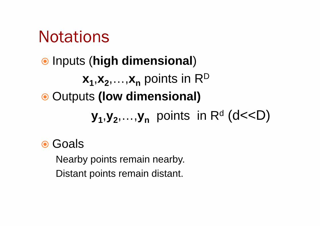
� Inputs (high dimensional)x1,x2,…,xn points in RD

� Outputs (low dimensional)

y ,y ,…,y points in Rd (d<<D) y1,y2,…,yn points in Rd (d<<D)

� GoalsNearby points remain nearby.Distant points remain distant.

Linear Methods

� PCA� MDS

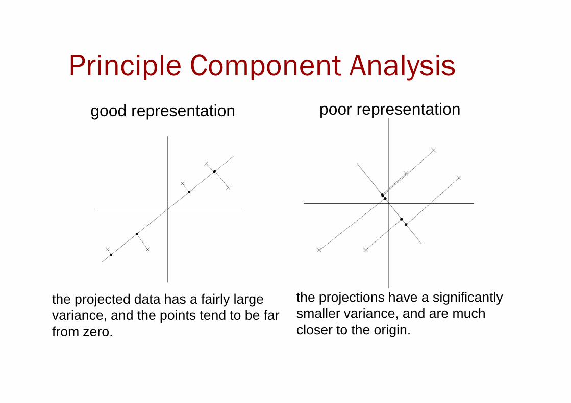
Principle Component Analysis

good representation poor representation

the projections have a significantly smaller variance, and are muchcloser to the origin.

the projected data has a fairly large variance, and the points tend to be far from zero.

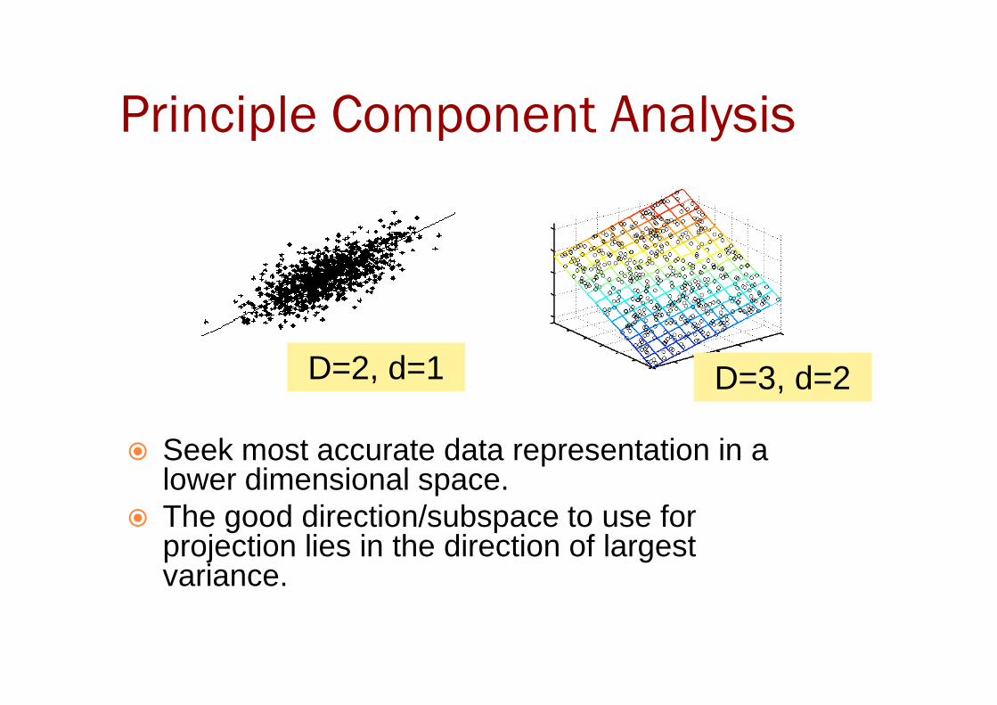
Principle Component Analysis

D=2, d=1

� Seek most accurate data representation in a lower dimensional space.

� The good direction/subspace to use for projection lies in the direction of largest variance.

D=2, d=1 D=3, d=2

Maximum Variance Subspace

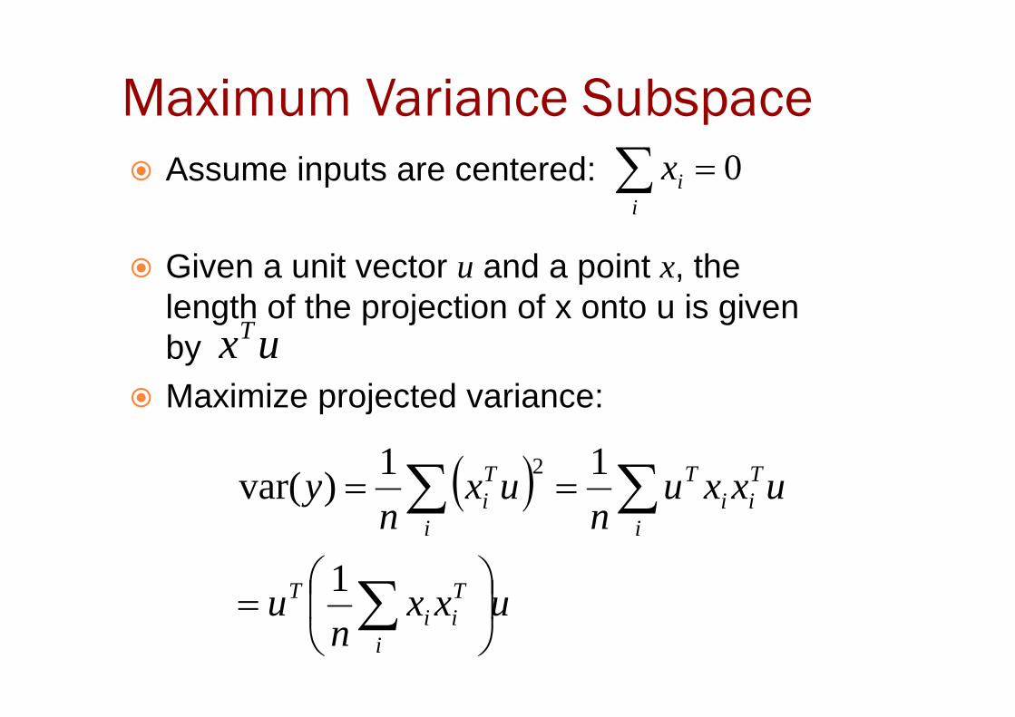
� Assume inputs are centered:

� Given a unit vector u and a point x, the length of the projection of x onto u is given by

0=∑i

ix

uxTby

� Maximize projected variance:

ux

( )

uxxn

u

uxxun

uxn

y

i

Tii

T

i

Tii

T

i

Ti

=

==

∑

∑∑

1

11)var(

2

1D Subspace

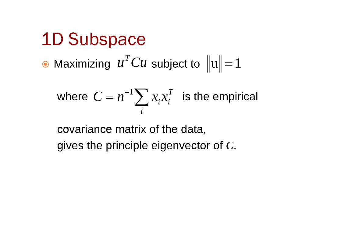
� Maximizing subject to

where is the empirical

CuuT

Ti

ii xxnC ∑−= 1

1u =

covariance matrix of the data,gives the principle eigenvector of C.

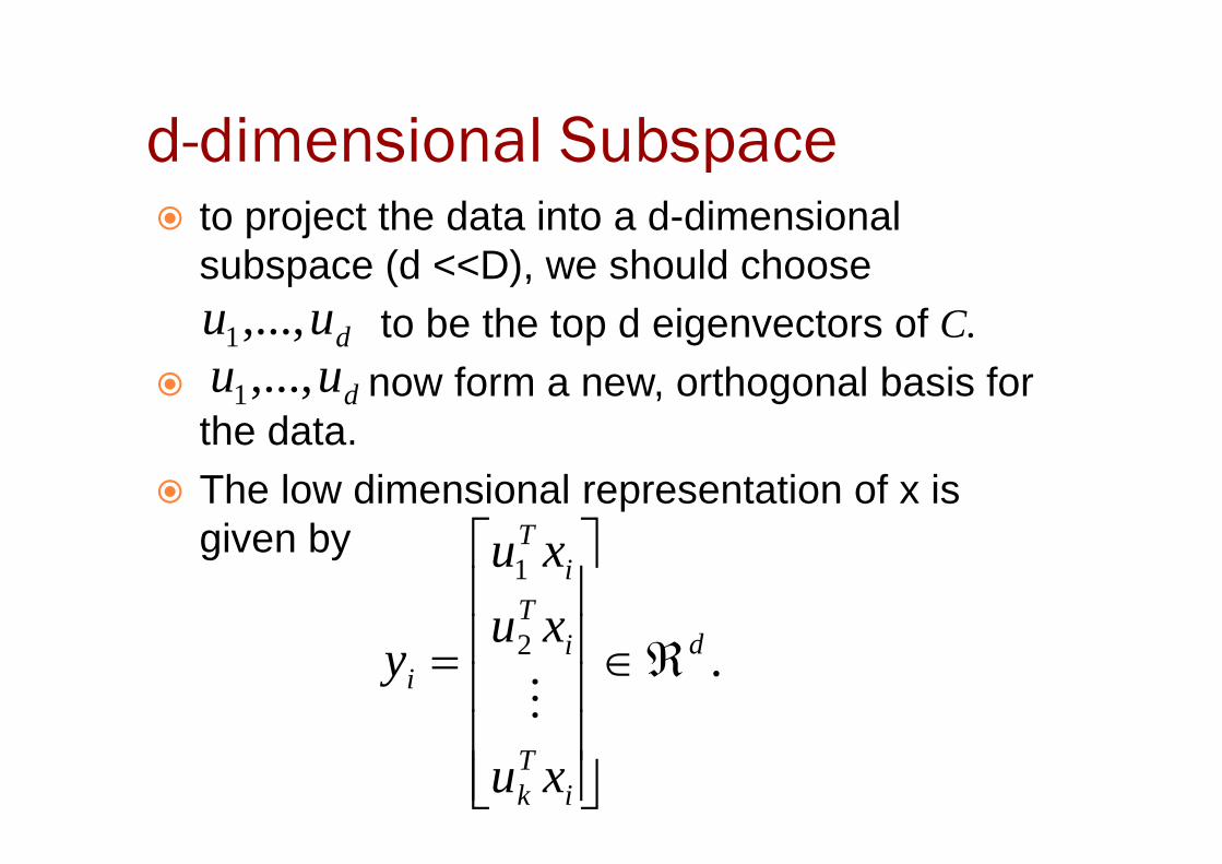
d-dimensional Subspace� to project the data into a d-dimensional

subspace (d <<D), we should chooseto be the top d eigenvectors of C.

� now form a new, orthogonal basis for the data.

duu ,..., 1

duu ,..., 1the data.

� The low dimensional representation of x is given by

. 2

1

d

iTk

iT

iT

i

xu

xu

xu

y ℜ∈

=M

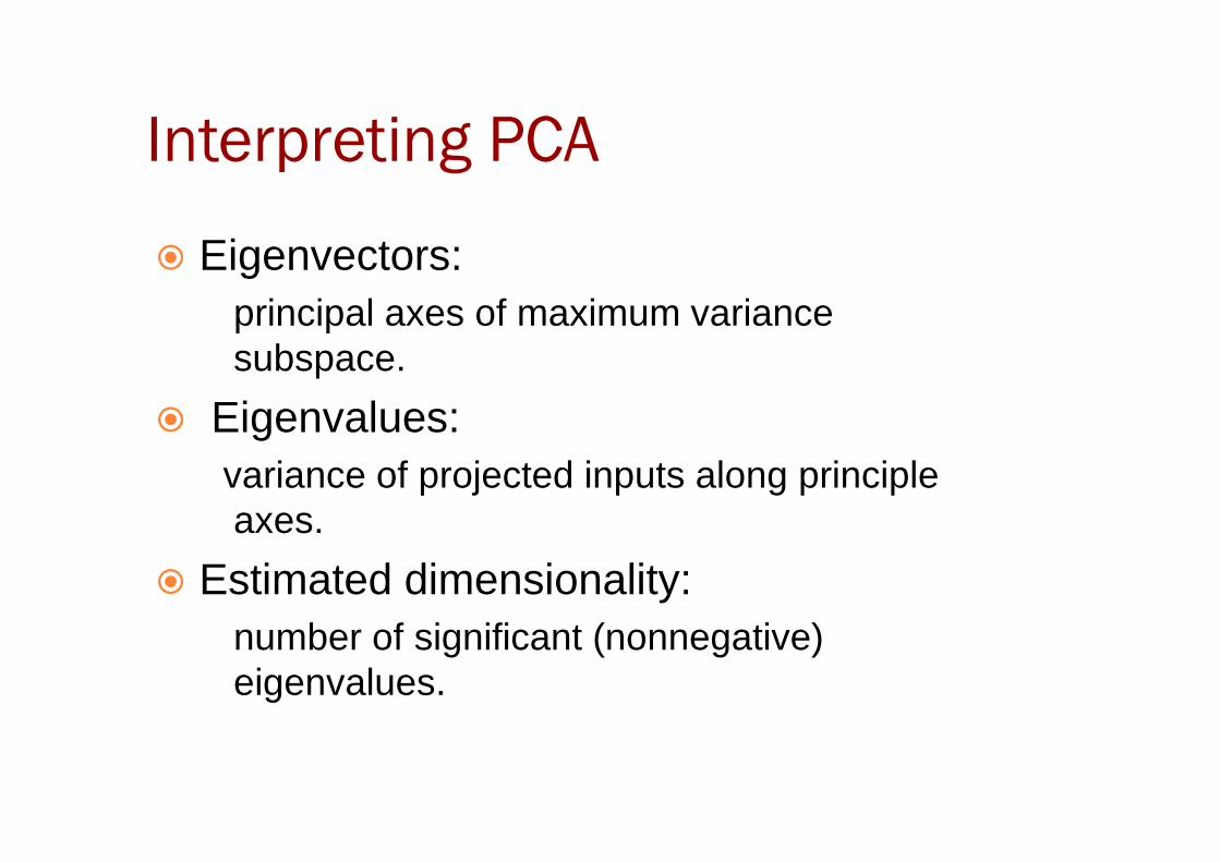
Interpreting PCA

� Eigenvectors:principal axes of maximum variance subspace.

� Eigenvalues:� Eigenvalues:variance of projected inputs along principle axes.

� Estimated dimensionality:number of significant (nonnegative) eigenvalues.

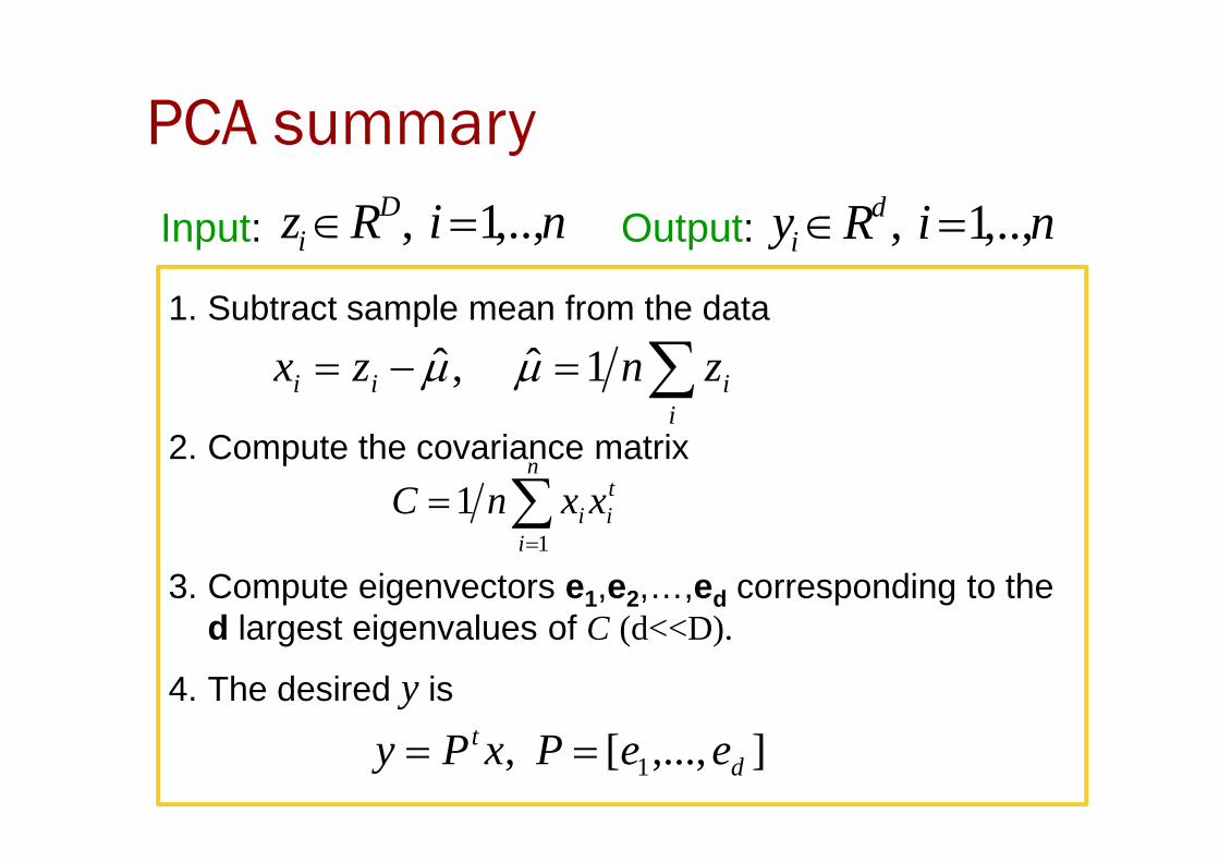
PCA summary

1. Subtract sample mean from the data

2. Compute the covariance matrix

∑=−=i

iii znzx 1ˆ ,ˆ µµ

Input: Output: niRz Di ,..,1 , =∈ niRy d

i ,..,1 , =∈

2. Compute the covariance matrix

3. Compute eigenvectors e1,e2,…,ed corresponding to the d largest eigenvalues of C (d<<D).

4. The desired y is

∑=

=n

i

tii xxnC

1

1

],...,[ , 1 dt eePxPy ==

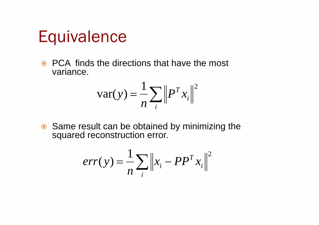
Equivalence

� PCA finds the directions that have the most variance.

21)var( ∑=

ii

T xPn

y

� Same result can be obtained by minimizing the squared reconstruction error.

21)( ∑ −=

ii

Ti xPPx

nyerr

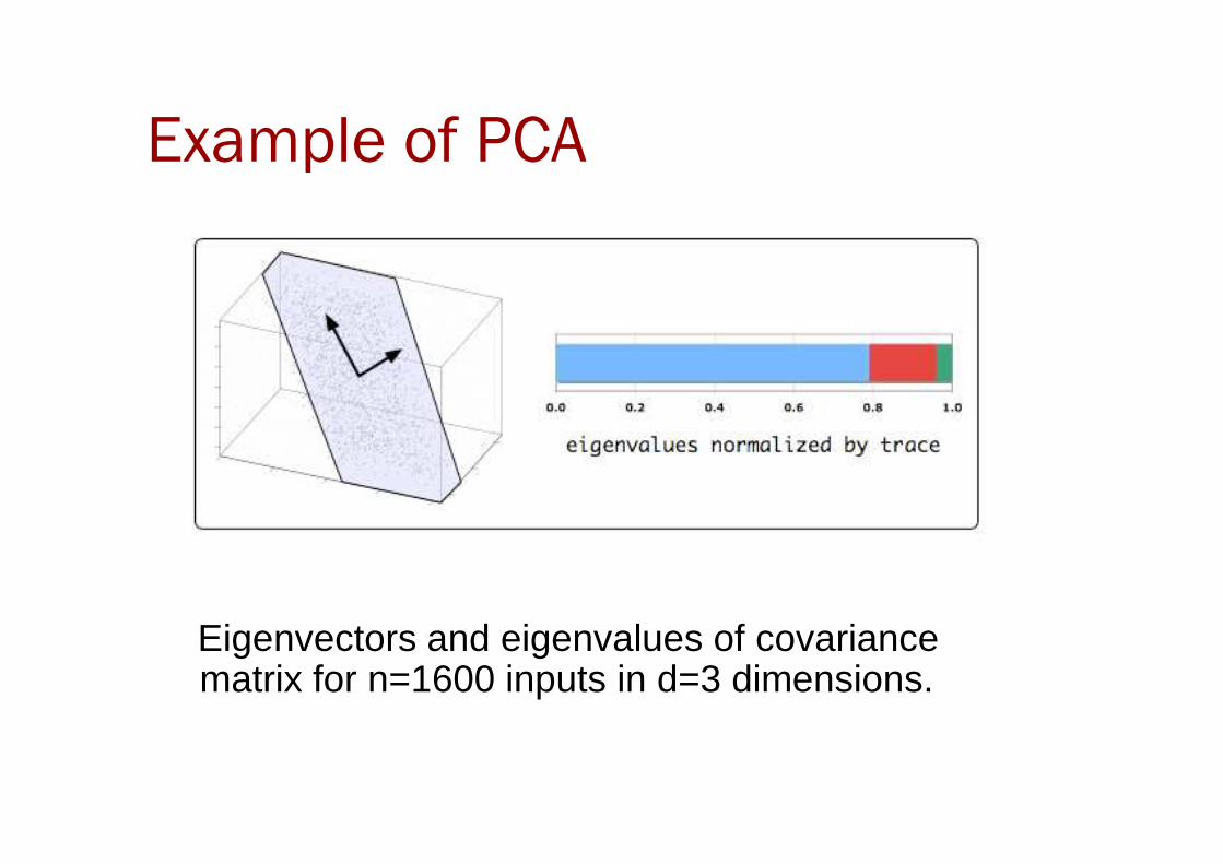
Example of PCA

Eigenvectors and eigenvalues of covariance matrix for n=1600 inputs in d=3 dimensions.

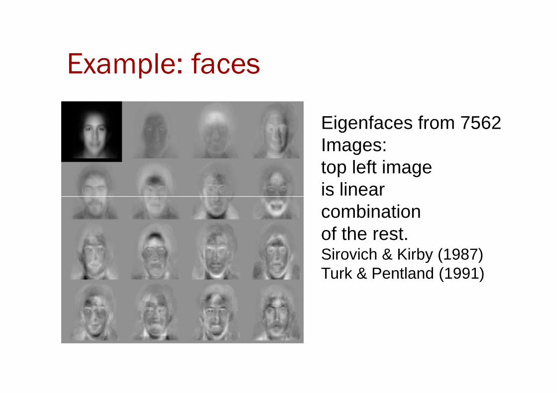
Example: faces

Eigenfaces from 7562Images:top left imageis linearis linearcombinationof the rest.Sirovich & Kirby (1987)Turk & Pentland (1991)

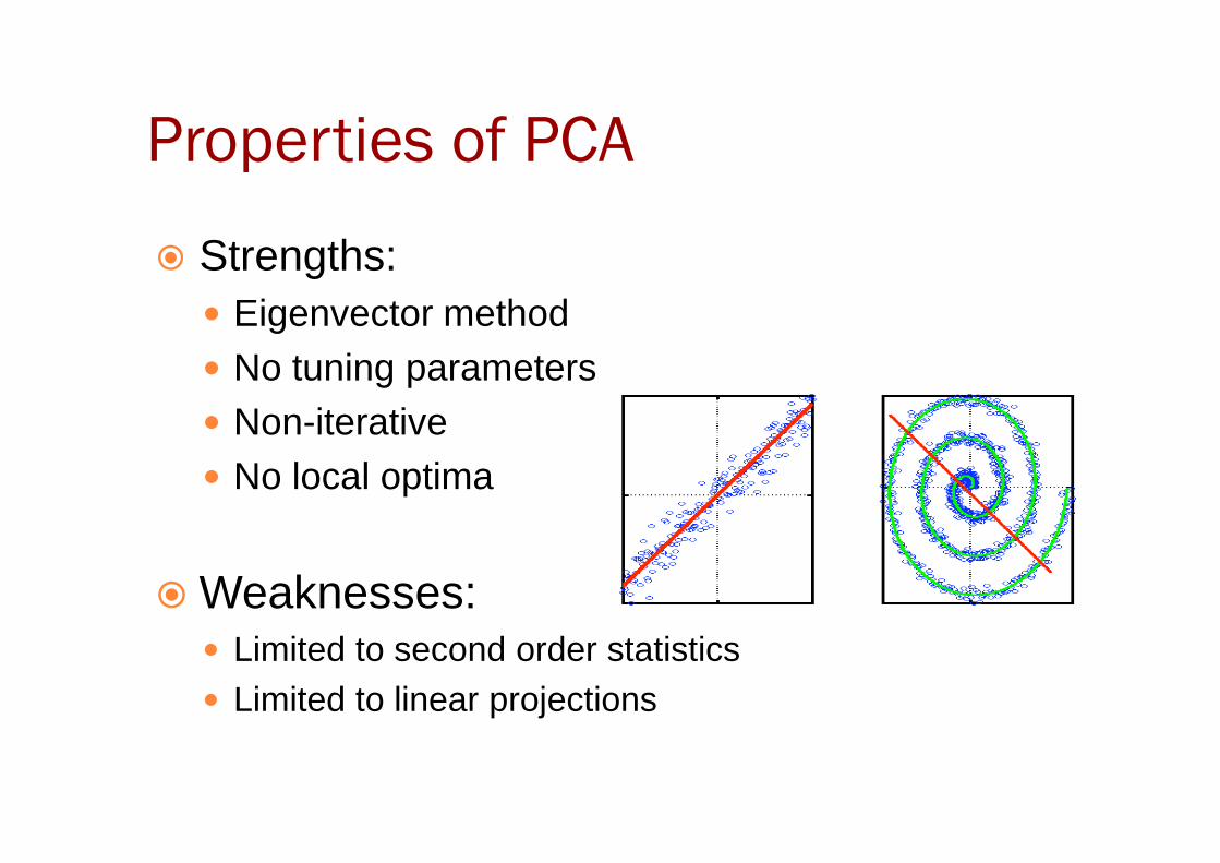
Properties of PCA

� Strengths:� Eigenvector method� No tuning parameters� Non-iterative� Non-iterative� No local optima

� Weaknesses:� Limited to second order statistics� Limited to linear projections

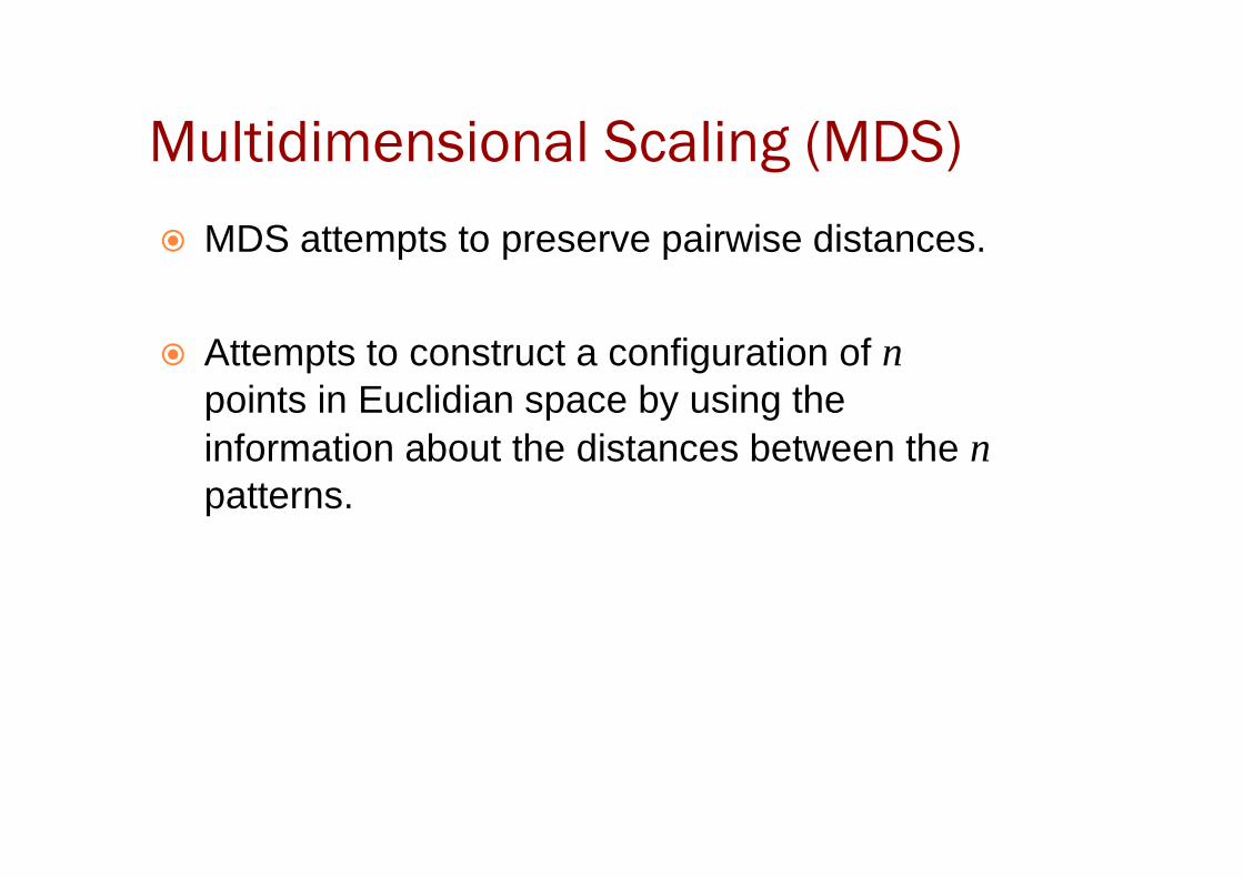
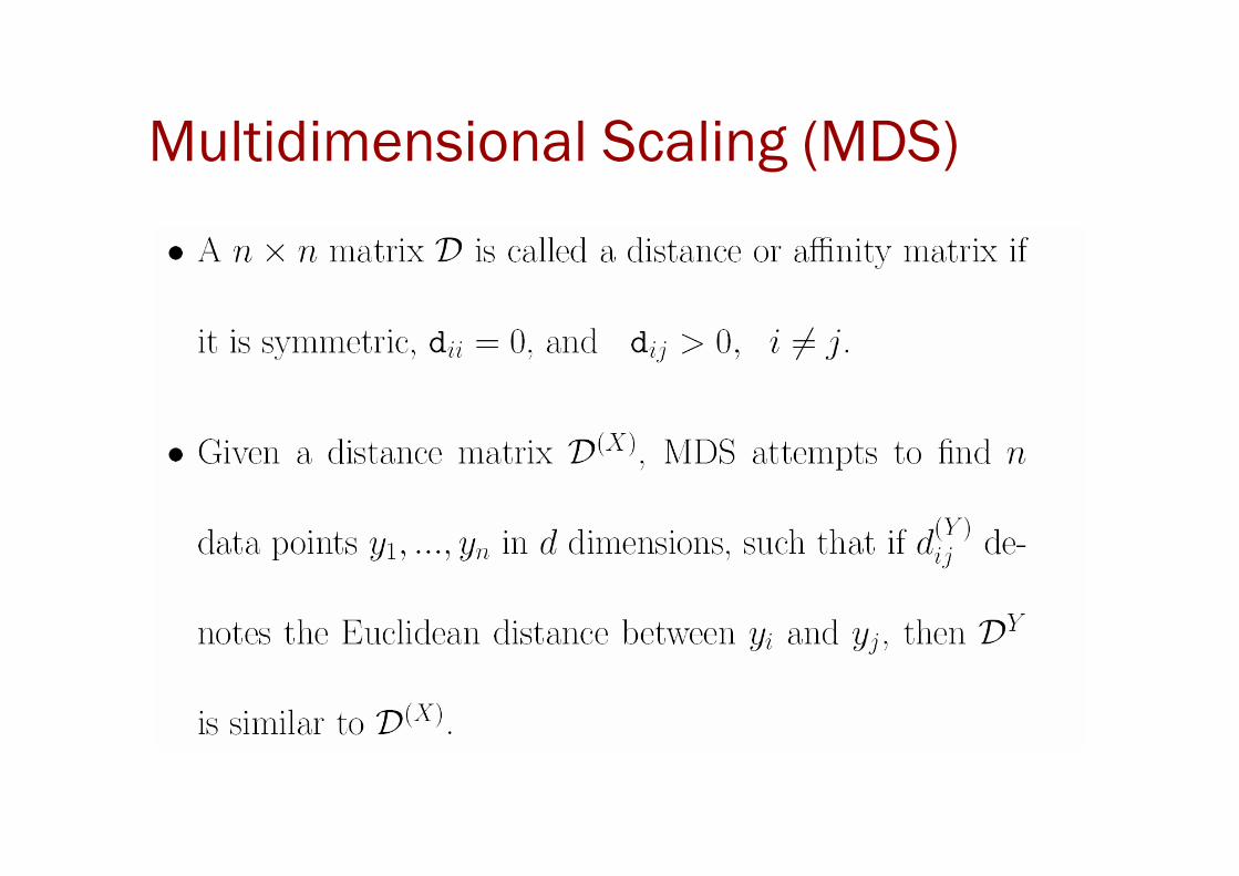
Multidimensional Scaling (MDS)

� MDS attempts to preserve pairwise distances.

� Attempts to construct a configuration of n points in Euclidian space by using the information about the distances between the ninformation about the distances between the npatterns.

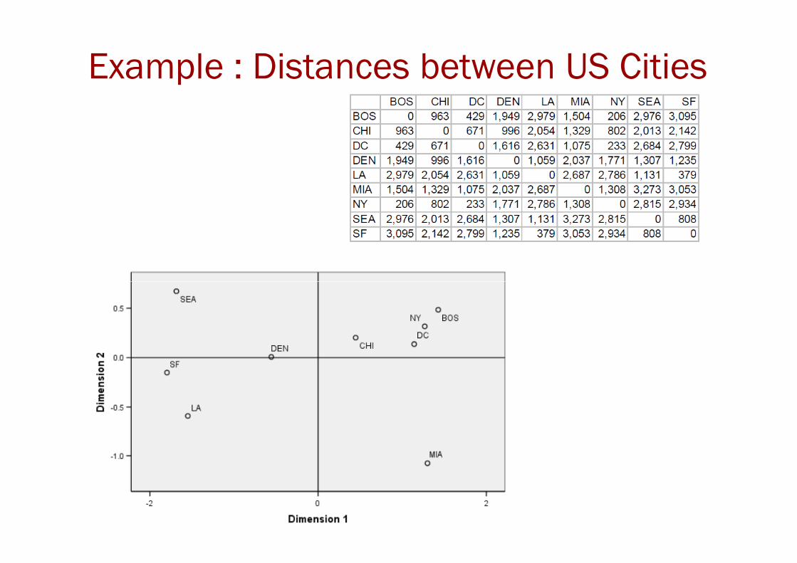
Example : Distances between US Cities

Multidimensional Scaling (MDS)

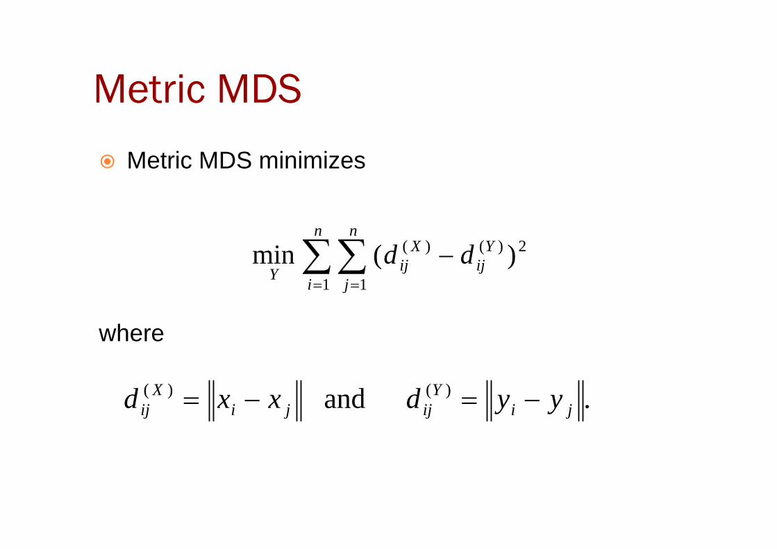
Metric MDS

� Metric MDS minimizes

∑∑= =

−n n

Yij

Xij

Ydd 2)()( )(min

where

∑∑= =i j

Y1 1

. and )()(ji

Yijji

Xij yydxxd −=−=

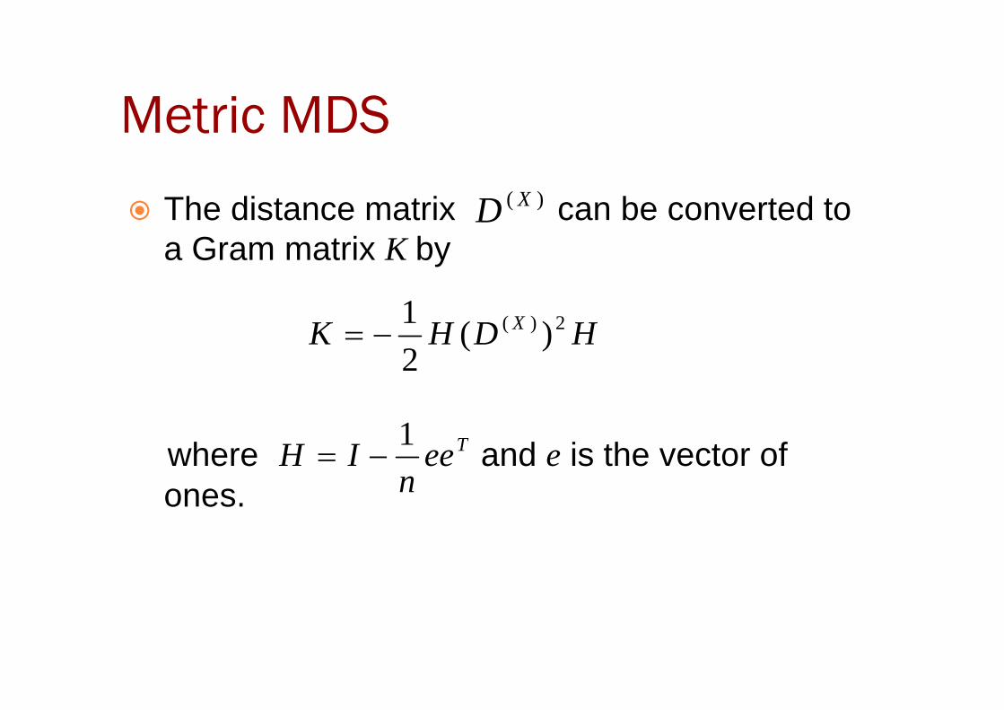
Metric MDS

� The distance matrix can be converted to a Gram matrix K by

)( XD

HDHK X 2)( )(2

1−=

where and e is the vector of ones.

2

Teen

IH1

−=

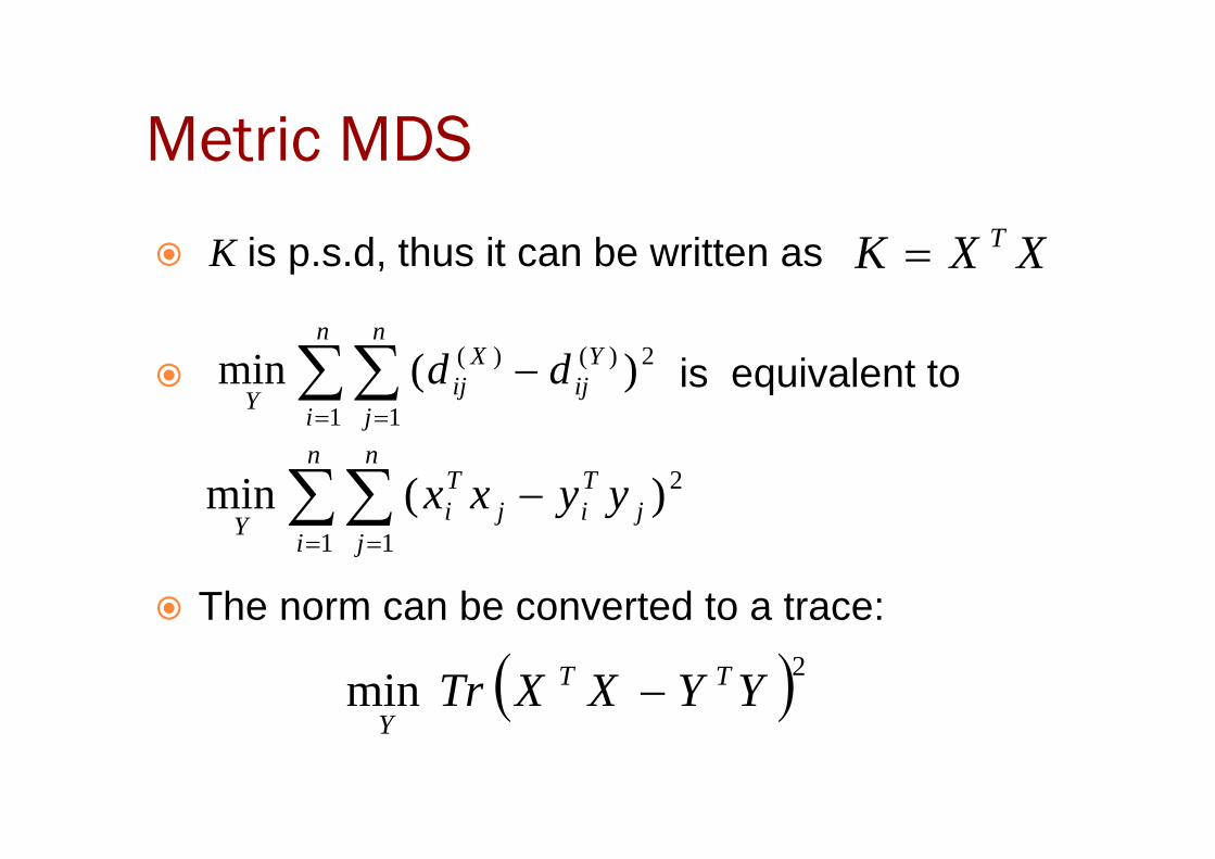
Metric MDS

� K is p.s.d, thus it can be written as

� is equivalent to

XXK T=

∑∑= =

−n

i

n

j

Yij

Xij

Ydd

1 1

2)()( )(min

� The norm can be converted to a trace:

= =i j1 1

∑∑= =

−n

i

n

jj

Tij

Ti

Yyyxx

1 1

2)(min

( )2min YYXXTr TT

Y−

Metric MDS

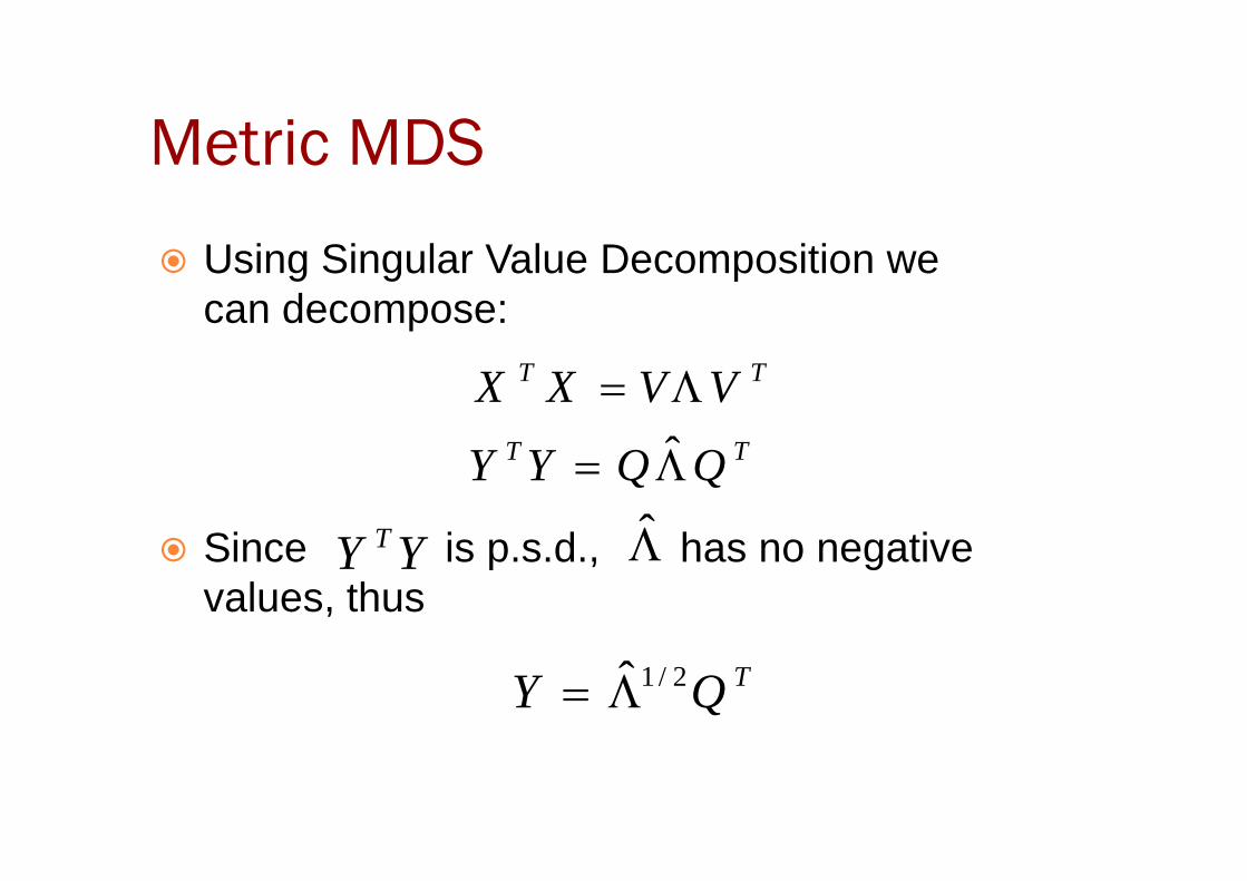
� Using Singular Value Decomposition we can decompose:

TT

TT

QQYY

VVXX

Λ=

Λ=

ˆ

� Since is p.s.d., has no negative values, thus

TT QQYY Λ= ˆ

YY T Λ̂

TQY 2/1Λ̂=

Metric MDS

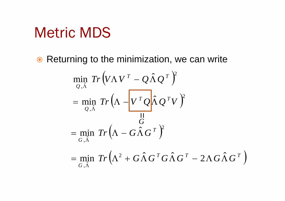
� Returning to the minimization, we can write

( )( )2

2

ˆ,

ˆmin

ˆmin

VQQVTr

QQVVTr

TT

TT

Q

Λ−Λ=

Λ−ΛΛ

( )ˆ,

ˆmin VQQVTr TT

QΛ−Λ=

Λ

G

( )2ˆ,

ˆmin T

GGGTr Λ−Λ=

Λ=

( )TTT

GGGGGGGTr ΛΛ−ΛΛ+Λ=

Λ

ˆ2ˆˆmin 2

ˆ,

Metric MDS

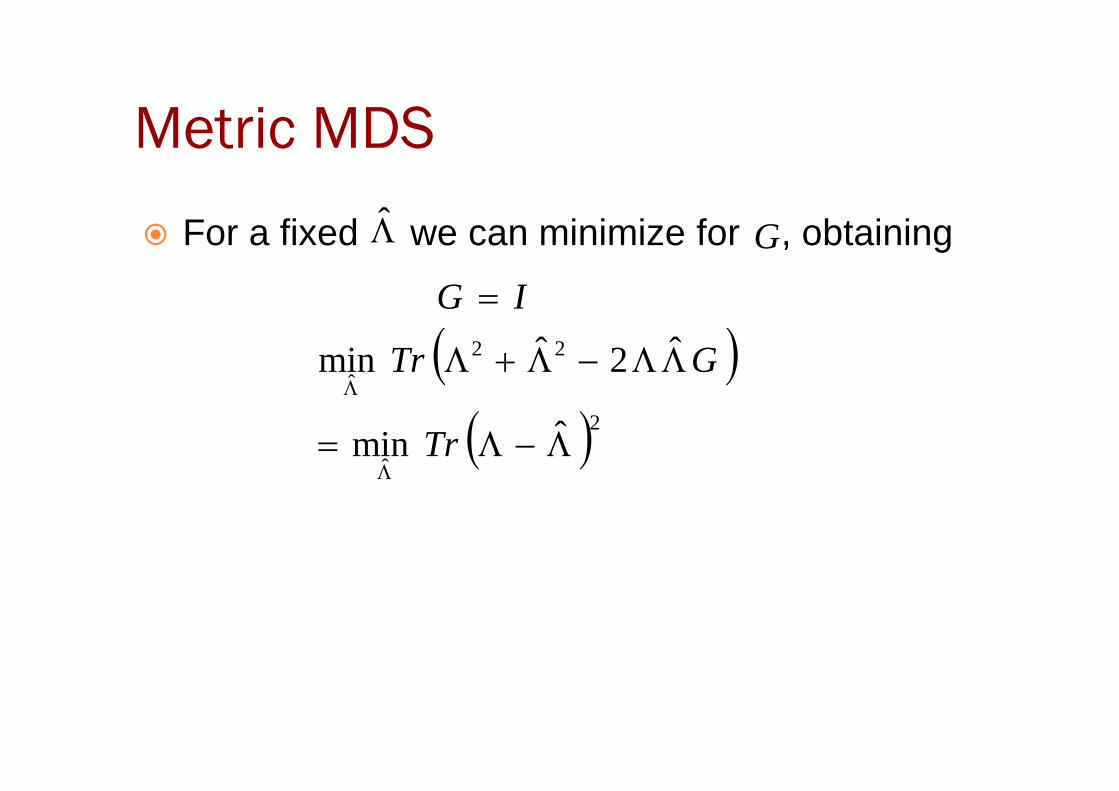
� For a fixed we can minimize for , obtaining Λ̂ G

IG =

( )( )

22

ˆˆ2ˆmin ΛΛ−Λ+Λ

ΛGTr

( )2ˆ

ˆmin Λ−Λ=Λ

Λ

Tr

Metric MDS

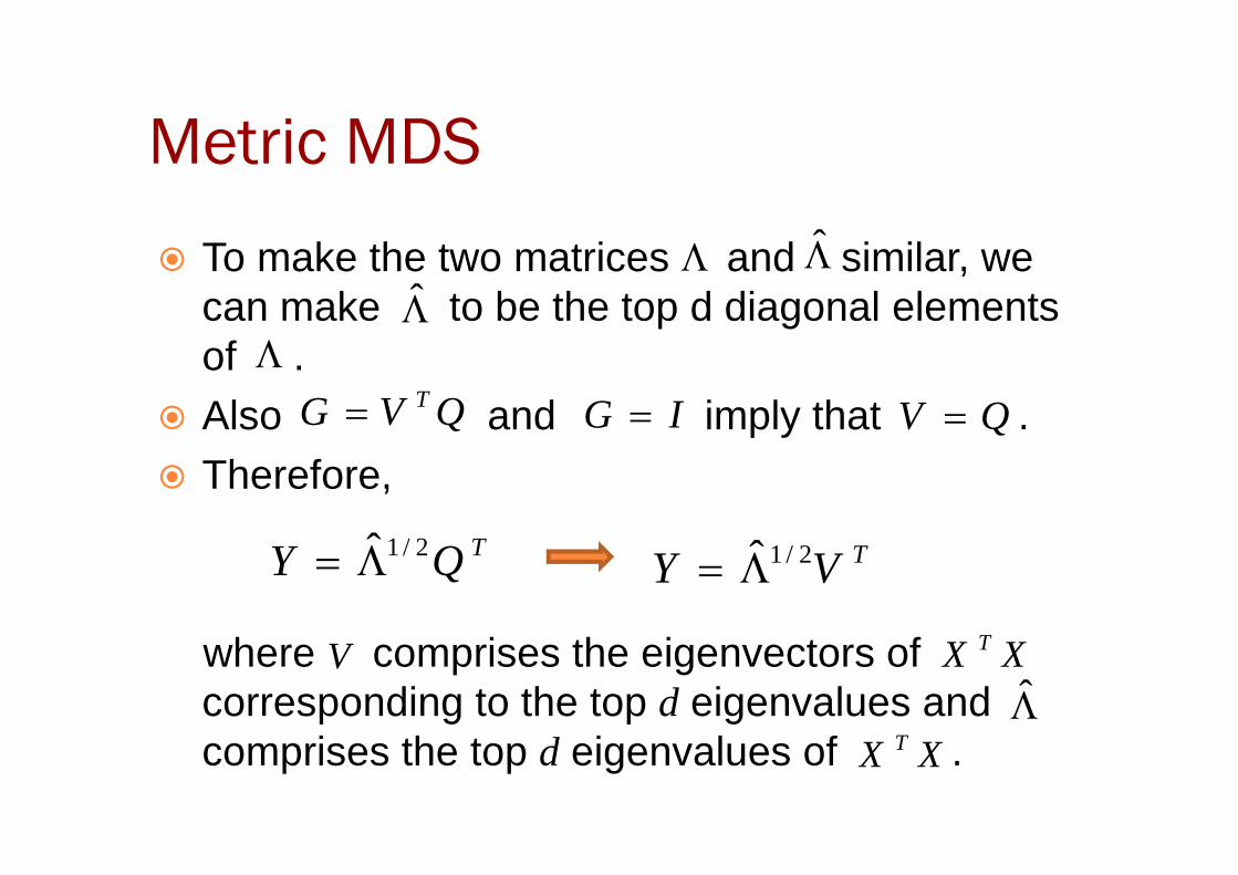
� To make the two matrices and similar, we can make to be the top d diagonal elements of .

� Also and imply that .

Λ

QVG T=

Λ̂Λ̂

Λ

IG = QV =Also and imply that .� Therefore,

where comprises the eigenvectors of corresponding to the top d eigenvalues and comprises the top d eigenvalues of .

QV =

TQY 2/1Λ̂= TVY 2/1Λ̂=

V XX T

Λ̂XX T

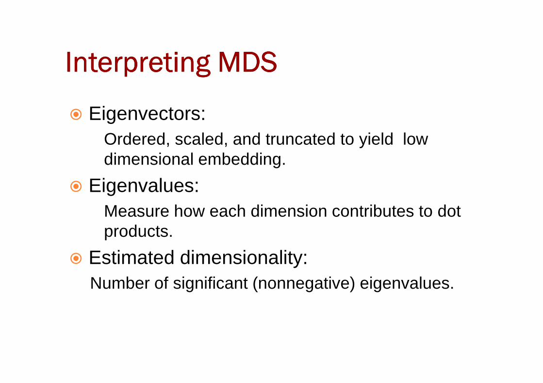
Interpreting MDSInterpreting MDSInterpreting MDSInterpreting MDS

� Eigenvectors:Ordered, scaled, and truncated to yield low dimensional embedding.

� Eigenvalues:� Eigenvalues:Measure how each dimension contributes to dot products.

� Estimated dimensionality:Number of significant (nonnegative) eigenvalues.

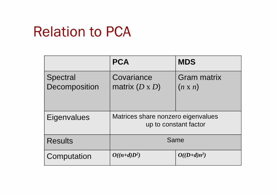
Relation to PCA

PCA MDS

Spectral Decomposition

Covariancematrix (D x D)

Gram matrix(n x n)

Eigenvalues Matrices share nonzero eigenvaluesup to constant factor

Results Same

Computation O((n+d)D2) O((D+d)n2)

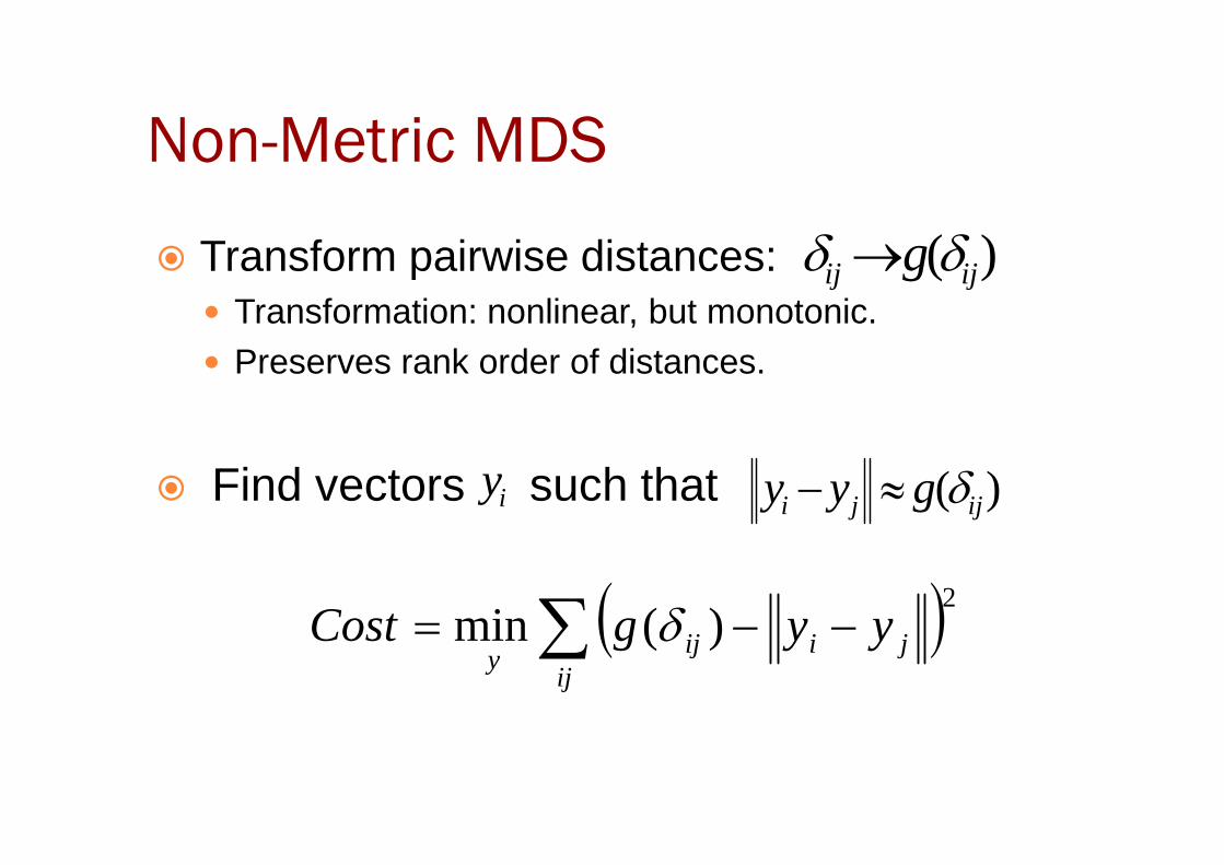
Non-Metric MDS

� Transform pairwise distances:� Transformation: nonlinear, but monotonic.� Preserves rank order of distances.

)( ijij g δδ →

� Find vectors such thatiy )( ijji gyy δ≈−

( )∑ −−=ij

jiijy

yygCost2

)(min δ

Non-Metric MDS

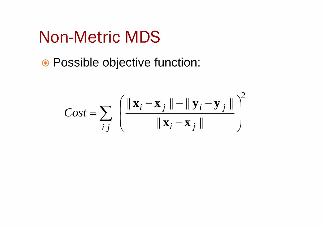
� Possible objective function:

2||||||||

−

−−−=∑ jijiCost

yyxx

||||

−

=∑jiji

Costxx

Properties of non-metric MDS

� Strengths� Relaxes distance constraints.� Yields nonlinear embeddings.

� Weaknesses� Weaknesses� Highly nonlinear, iterative optimization with

local minima.� Unclear how to choose distance

transformation.