UNIVERSITÀ POLITECNICA DELLE MARCHE __________________________________________________________________________________________________________________________________________________________________

DIPARTIMENTO DI SCIENZE ECONOMICHE E SOCIALI

AGRICULTURAL PRICE TRANSMISSION ACROSS SPACE AND COMMODITIES DURING PRICE

BUBBLES

ROBERTO ESPOSTI AND GIULIA LISTORTI

QUADERNO DI RICERCA n. 367*

Novembre 2011

Comitato scientifico:

Renato Balducci Marco Gallegati Alberto Niccoli Alberto Zazzaro Collana curata da: Massimo Tamberi

* La numerazione progressiva continua dalla serie denominata: Quaderni di Ricerca - Dipartimento di Economia

AGRICULTURAL PRICE TRANSMISSION

ACROSS SPACE AND COMMODITIES DURING

PRICE BUBBLES

Roberto Esposti♣ and Giulia Listorti♦

Abstract

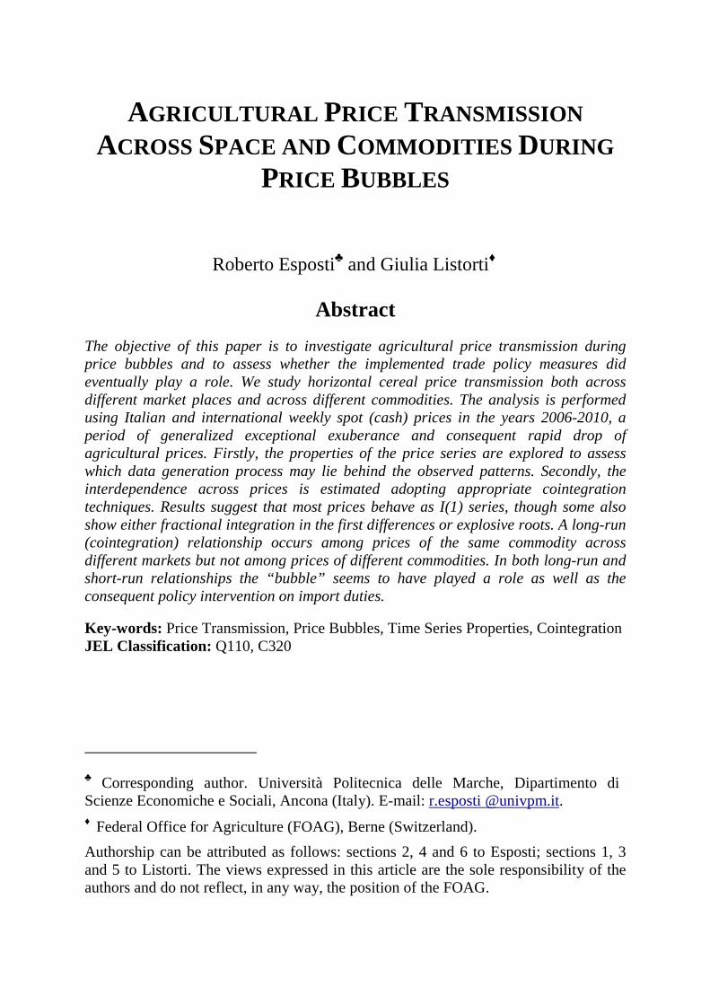
The objective of this paper is to investigate agricultural price transmission during price bubbles and to assess whether the implemented trade policy measures did eventually play a role. We study horizontal cereal price transmission both across different market places and across different commodities. The analysis is performed using Italian and international weekly spot (cash) prices in the years 2006-2010, a period of generalized exceptional exuberance and consequent rapid drop of agricultural prices. Firstly, the properties of the price series are explored to assess which data generation process may lie behind the observed patterns. Secondly, the interdependence across prices is estimated adopting appropriate cointegration techniques. Results suggest that most prices behave as I(1) series, though some also show either fractional integration in the first differences or explosive roots. A long-run (cointegration) relationship occurs among prices of the same commodity across different markets but not among prices of different commodities. In both long-run and short-run relationships the “bubble” seems to have played a role as well as the consequent policy intervention on import duties.

Key-words: Price Transmission, Price Bubbles, Time Series Properties, Cointegration JEL Classification: Q110, C320

♣ Corresponding author. Università Politecnica delle Marche, Dipartimento di Scienze Economiche e Sociali, Ancona (Italy). E-mail: r.esposti @univpm.it. ♦ Federal Office for Agriculture (FOAG), Berne (Switzerland).

Authorship can be attributed as follows: sections 2, 4 and 6 to Esposti; sections 1, 3 and 5 to Listorti. The views expressed in this article are the sole responsibility of the authors and do not reflect, in any way, the position of the FOAG.

Contents 1. Introduction: objectives and data description _________________________1

2. Some basic evidence on agricultural price behaviour ___________________3

2.1. Stationarity ______________________________________________3

2.2. Long memory (fractional integration) _________________________5

2.3. Testing explosiveness: recursive unit root tests __________________6

3. Modelling price interdependence as price transmission mechanisms _______8

3.1. A general model of price transmission_________________________8

3.2. Model specification ______________________________________10

3.3. Structural breaks: the bubble and the policy regime switching _____13

4. Econometric procedure _________________________________________13

5. Results______________________________________________________15

5.1. Cross-market transmission _________________________________15

5.2. Cross-commodity transmission _____________________________17

6. Some final remarks ____________________________________________18

References_____________________________________________________21

ANNEX 1 – Price commodities and groups under analysis _______________29

ANNEX 2 – Unit and explosive roots testing __________________________30

1

Agricultural Price Transmission Across Space and Commodities

During Price Bubbles

1. Introduction: objectives and data description

The analysis of agricultural price transmission during intense market turmoil represents a

major research challenge. The investigation may be empirically problematic due to the

particular stochastic properties assumed by the price series during these periods of turbulence;

however, it is clear that studying the co-movement of prices under these conditions is

particularly useful to understand to which extent prices are linked together. The main

motivation of the present study is to investigate the properties of agricultural price series over

the recent price rally (European Commission, 2008; Irwin and Good, 2009)1 to better analyse

how price shocks were transmitted horizontally, that is across market places and commodities.

We use cereal weekly spot prices from May 2006 to December 2010. We opt for this time

coverage for three major reasons. Firstly, this period fully contains the bubble: the bubble

firstly inflated, then completely deflated and finally started raising again in the second half of

2010 (Figure 1). Secondly, we can assume an almost-constant policy regime in the European

Union (EU). In 2006, the 2003 reform of the Common Agricultural Policy (CAP) was entirely

in place, included its limited implications in terms of price policy and market intervention; we

can then assume that the domestic policy regime remained constant over the years 2006-2010.

Concerning international trade policy, the only relevant policy regime change has been the

temporary suspension of EU import duties on cereals from January 2008 to October 2008, as

a reaction to the exceptionally tight situation on world markets. This temporary measure

might have altered the price transmission mechanisms. Therefore, while investigating price

transmission during the bubble, it is also possible to assess the role played by this single and

temporary policy measure. Thirdly, concentrating on this period facilitates international price

comparisons as the cumulative inflation rate has been quite limited and relatively similar in

Italy and in North-America (the two areas under study here). Therefore, comparisons of

agricultural prices across different countries do not require the deflation of nominal prices

into a common real base.

1 Henceforth, the “agricultural price bubble”. Heuristically, and generically, the bubble clearly appears in Figure 1. From a more rigorous point of view, however, we will formally define and test the presence of a price bubble in section 2.3.

2

We analyse weekly spot price series observed in different Italian locations (from North to

South; source: ISMEA) and international (North-American) markets (source: International

Grain Council, IGC) (Esposti and Listorti, 2011). The reason why we focus on durum wheat

and corn is that they represent somehow opposite cases. Amongst the main cereals, durum

wheat experienced the largest price rise (and, then, decline) during the bubble, while corn

prices showed the smallest variation (see Figure 1 and Esposti and Listorti, 2011). Comparing

these two extreme cases is particularly insightful to understand whether some common

features of the price movements can be found even across commodities showing quite diverse

market fundamentals. Significant differences between durum wheat and corn may be found

on both the demand and the supply side, at least in the Italian case. On the demand side, the

prevailing domestic (Italian) uses are very different for the two cereals: almost exclusively

human consumption for durum wheat, prevalent feed use for corn. Therefore, we can deduce a

pretty limited interdependence among them, since they behave neither as strong complements

nor as strong substitutes. On the supply side, Italy is the largest EU durum wheat producing

country (durum wheat is one of the characteristic products of the Italian agriculture) while, on

the contrary, corn is a less typical production. Therefore, we can presume a different linkage

between the national and the international prices in the two cases.

The dataset has a Tx(NxK) dimension where: T=244 weeks (from the first week of May 2006

to the last week of December 2010); K=2 commodities (durum wheat and corn); N=5 market

places, that is, North-Italy (Milan), Centre-North Italy (Bologna), Centre-South Italy (Rome),

South-Italy (Foggia), US and Canada (or Rotterdam; see below). The codification and

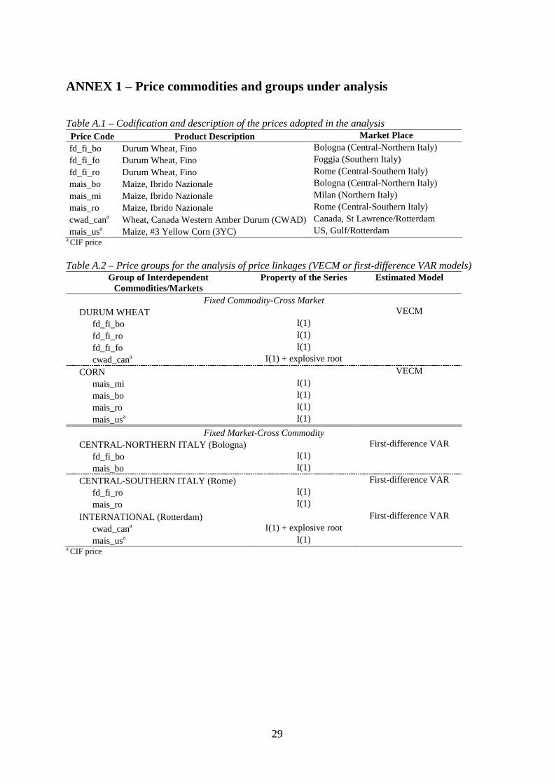
description of the NxK=10 price series under investigation are reported in Table A.1 (Annex

1).

The North-American prices are FOB prices. For agricultural commodities, freight rates are

normally quite relevant. Moreover, due to volatility in energy, namely oil, prices, they also

considerably oscillated during the commodity price bubble. For these reasons, freight rates

(source: IGC) were added to US and Canadian prices in order to obtain the respective CIF

prices. The freight rates used in this study are those from US Gulf (or Canada, where

applicable) to Amsterdam/Rotterdam/Antwerp/Hamburg destinations. In practice, in our

analysis the North-American prices actually serve as international prices taken at Rotterdam,

thus as EU-reference prices. Henceforth, we will also refer to international prices as

Rotterdam prices (Table A.1). These US and Canadian CIF prices have been finally converted

3

from US dollars to Euros by using the weekly official $/€ exchange rate provided by Eurostat-

ECB.2

2. Some basic evidence on agricultural price behaviour

Before analysing price interactions and the reciprocal transmission of price shocks, the time

series properties of the data have been assessed. This allows identifying the common features

of the price series, in order to achieve a proper specification of price

transmission/interdependence relations.

Let us consider agricultural prices observed over three different dimensions: space,

commodity and time. Therefore, the generic price is tkip ,, where: i=1,…,j,…,N is the (local)

market place (spatial dimension); k=1,…,h,…,K is the commodity; t=1,…,s,…,T is the period

of observation (time dimension). By more conventionally distinguishing between a cross-

sectional dimension, given by the combination of the dimensions ik, and a time dimension t,

we can identify any generic price observation as tikp , (scalar) and any generic price series

(vector) as ikp . The logarithms of prices are here considered. This monotonic transformation

facilitates the economic interpretation of results, in particular considering that regression

coefficients may be interpreted as elasticities. Therefore, henceforth ikp identifies the time

series of the price logarithm of the k-th commodity in the i-th market place.

The time-series properties of the prices are analysed in the following sections by testing, in

sequence, stationarity, persistence (long memory or fractional integration) and explosiveness

to assess whether these features may be invoked as possible causes of the observed

exuberance.3

2.1. Stationarity

The presence of unit and/or explosive roots is critical to understand the behaviour of price

series especially in periods of such dramatic exuberance and drop. Stationary (i.e. I(0)) series

can be hardly reconciled with the presence of the bubble. Even stationarity around a drift (a

constant term) and/or a deterministic trend is not evidently helpful in this respect. As clarified

below, testing for the presence of a temporary explosive pattern cannot be simply achieved

2 Using prices already converted in the same currency is a widely used procedure; it follows that adjustment to the exchange rate is assumed instantaneous. 3 Other time-series properties that could generate non-linear dynamics in price patterns, in particular non-normality and seasonality, have been tested and generally excluded (see Esposti and Listorti, 2011, for more details).

4

through conventional unit-root tests. Nonetheless, albeit not sufficient, these tests still allow

to assess a necessary outcome of nonlinearities within price series: the series are expected to

be I(1) and not I(0) (Diba and Grossman, 1988; Evans, 1991; Phillips and Magdalinos, 2009;

Philips et al., 2009; Phillips and Yu, 2009).

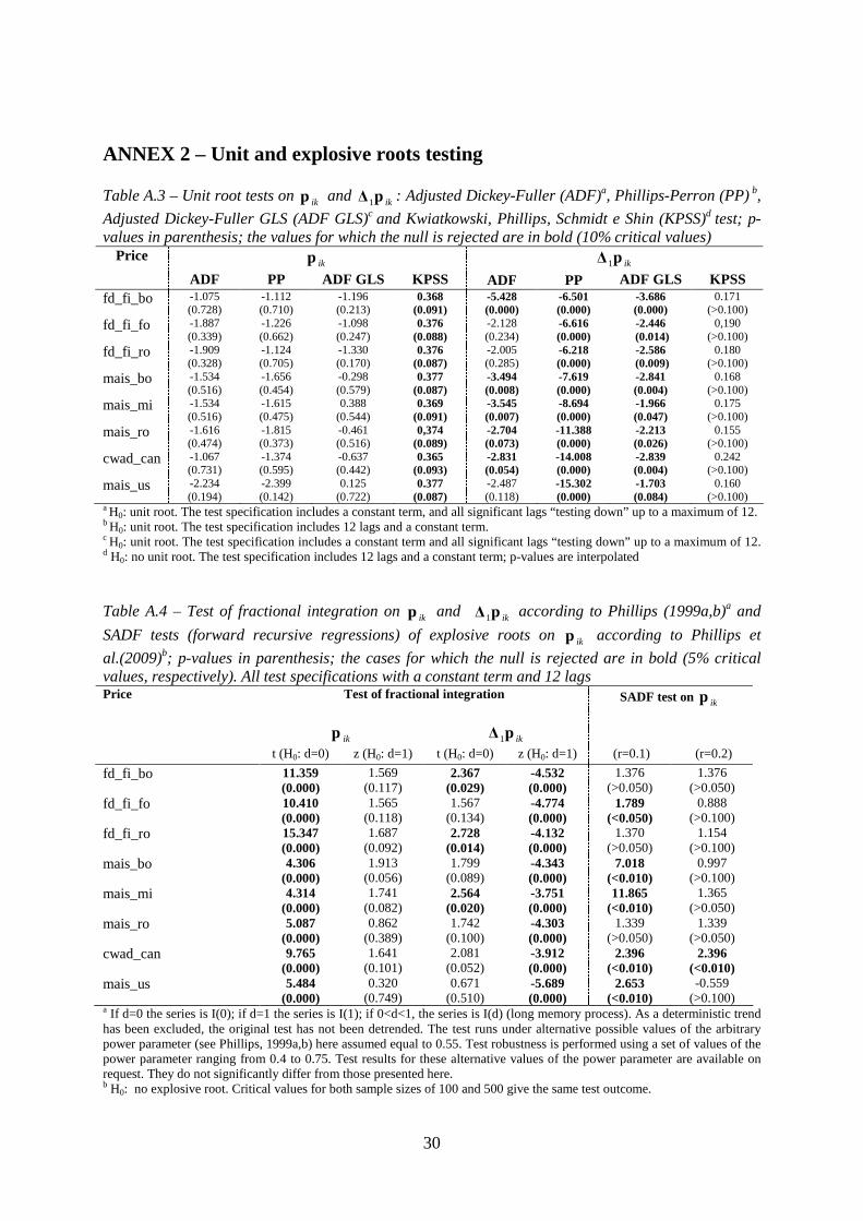
Table A.3 (Annex 2) reports unit root tests on ikp and on their respective first differences,

ikp∆1 . Four different unit-root tests are run (Enders, 1995; Stock and Watson, 2011). The first

is the conventional ADF (Adjusted Dickey-Fuller) test. This test, however, encounters known

limitations particularly for series like those under consideration here and, thus, may provide

misleading evidence on their underlying stochastic properties. The second test is the PP

(Phillips-Perron) test, that is expected to be more robust than the ADF test under

heteroskedasticity which may, in fact, occur during periods of exuberance. Furthermore, two

other tests are performed, both aiming at taking into account that the conventional ADF test

tends to accept the null hypothesis of unit root also for series that are, in fact, only “near unit

root” processes. This latter case is likely to occur in the price series under consideration here,

especially in their first differences. Firstly, an ADF-GLS test is performed. This modified

ADF test has significantly greater power than the conventional test especially under near unit

root processes and small sample size. Secondly, a KPSS test (Kwiatkowski, Phillips, Schmidt

and Shin) is performed. In this test, the null hypothesis is that the series is stationary, while

the alternative hypothesis is that it is I(1). Therefore, the KPSS test is expected to reveal those

series that the conventional ADF test tend to accept as I(1) while, in fact, they are only near

unit-root processes. The combination of these four unit-root tests should provide an

exhaustive picture on the real underlying stochastic processes of the price series thus allowing

for a robust and conclusive answer about their order of integration.

In general terms, looking at Table A.3 it seems that, once the proper specification has been

selected (in terms of number of lags and of the presence of drift and deterministic trend), all

ikp series show a unit root. If the conventional ADF test is considered, the evidence about the

ikp∆1 series is more mixed, though I(1) series still prevail on I(2). As mentioned, however,

conventional ADF tests may fail in detecting stationary series when their roots are near to

unity. The more robust PP, ADF-GLS and KPSS tests, in fact, show that all first differenced

series are stationary. The conclusion would be that all price series can be considered I(1) but

not I(2).

5

I(1) series (random walks possibly with a drift and/or a deterministic trend), however, are

apparently at odds with the evidence of a price bubble, as they can hardly generate the

temporary exuberance observed in all markets. Apparently, these prices are “something more”

than I(1) series. Two plausible explanations are the following. The first explanation is that

ikp∆1 , though I(0), may show long memory, therefore long persistence of shocks. A second

explanation is that temporary explosive roots (the “bubble”) actually occurred in ikp . As

conventional unit-root tests can not really assess (or exclude) these two hypotheses, ad hoc

tests are needed.

2.2. Long memory (fractional integration)

As emphasized by Wei and Leuthold (1998), agricultural prices (mostly, in fact, future prices)

are often characterised by long memory, which may also generate non-linear patterns quite

close to chaotic processes. In such cases, price series are neither I(0) nor I(1) but rather I(d)

processes, with 0<d<1 (hence the term “fractional integration”). Fractional integration implies

that price series, though not behaving as random walks (where shocks never vanish over

time), still keep the memory of a given shock for a long period. Roughly speaking, price

shocks decay very slowly over time. This kind of stochastic process is here of specific interest

since when fractional integration occurs in the first differences, then I(1) price series can

generate the observed nonlinearities. In such cases, though a unit root cannot be detected in

the first-differenced series, a long-memory process would still imply strong persistence of

shocks.

Unfortunately, conventional unit-root tests may fail in detecting such property: they assess

whether time series are I(0) or I(1) while, in fact, they are I(d). The presence of long memory

within the price series can instead be tested following the approach originally proposed by

Geweke and Porter-Hudak (1983) and then modified by Phillips (1999a,b). This test is based

on a particular representation of the stochastic process generating the price series ikp , or its

first differences ikp1∆ , called ARFIMA(p,d,q) (Autoregressive Fractionally Integrated

Moving Average) model, where p and q express, as usual, the orders of auto-regressive and

the moving-average parts, respectively, and d the order of (fractional) integration. The

procedure proposed by Phillips (1999a,b), and adopted here, tests the value of parameter d

then distinguishing stationary, unit-root and fractionally integrated processes. The procedure

produces two test statistics, one for the null d=0 and one for d=1. If d=0 is accepted the series

6

is stationary; if d=1 is accepted the series has an unit root. If both are rejected (namely,

0<d<1), then fractional integration (long memory) is accepted.

Results of these tests are reported in Table A.4 (Annex 2). They confirm that, when applied to

the original series, a unit root is evidently observed. When applied to first differences, the

presence of a unit root is always rejected but in three national markets (two for durum wheat,

one for corn) the presence of fractional integration cannot be excluded.

2.3. Testing explosiveness: recursive unit root tests

In time-series econometrics, nonlinear patterns can naturally emerge in non-stationary

variables whose first differences are fractionally integrated processes or, a fortiori, second-

order integrated, I(2), series (Engsted, 2006). Nonetheless, a price series showing a period of

explosive behaviour (a temporary, or periodically collapsing, bubble) is not necessarily an

I(2) series. On the contrary, a I(2) process would imply a permanent exuberance of prices

while, in fact, the observed bubble inflates and deflates within a relatively limited period of

time. In fact, bubbles induce a temporary explosive root in price series in addition to a unit

root. If this additional root is not appropriately considered, conventional testing may fail in

detecting the real underlying stochastic process (Evans, 1991).

Recent works by Phillips and Magdalinos (2009), Philips et al. (2009) and Phillips and Yu

(2009) have provided an appropriate framework for assessing the presence of an explosive

root within processes that would otherwise be ruled as I(1). They propose a test for the

presence of bubbles in which forward recursive ADF tests are run on the price series. These

sequential tests allow assessing period-by-period the possible nonstationarity of the price

series against an explosive alternative. The forward recursive test is based on a conventional

ADF regression where in the first recursion only To = [roT] observations are used, where ro is

a fraction of the total sample T.4 In subsequent regressions this initial data set is supplemented

by successive observations, each time using a sample of size Tr = [rT] for ro ≤ r ≤ 1. For any

recursive sub-sample Tr, the respective ADF test is computed. Of these forward recursive

ADF tests (ADFr), the test of explosiveness considers the maximum observed value:

[ ]r

rrADFsupSADF

1,0∈= . Under the null hypothesis of unit root (H0: ikρ =1) and against the right-

tailed alternative hypothesis of an explosive root (H1: ikρ >1), we accept that the series

contains an explosive root if the estimated test SADF is higher than the respective critical

4 The brackets in [ro T] indicate that the integer part of the argument is taken.

7

values (reported, for different sample sizes, in Phillips et al., 2009, and Phillips and Yu,

2009). Here, ro has been alternatively fixed at 0.10 (24 observations) and at 0.20 (48

observations) (see Phillips et al, 2009, and Phillips and Yu, 2009), and then incremented by

each single following observation.

These SADF tests have been performed on ikp including the constant term and 12 lags5.

Table A.4 (last two columns) reports the results of these tests for both r=0.10 and r=0.20. The

latter case, however, provides a more robust evidence since it uses larger sub-samples, thus

reducing the risk of poor test performance in the first runs of the recursive process.6 For this

reason, a restrictive 1% critical value is used to test the presence of explosive roots. On this

basis, we can conclude that a temporary explosive behaviour is definitely found only in

durum wheat international (Rotterdam) price. The presence of an explosive root is doubtful in

few cases, while it can be excluded in all other price series.

This kind of test may be particularly helpful also to understand the timing of price exuberance

to eventually date the beginning and the end of the price bubble. To locate the origin and the

conclusion of the exuberance, one can display the series of the above mentioned forward

recursive ADFr test and check if and when ADFr exceeds the right-tailed critical values of the

asymptotic distribution of the standard Dickey–Fuller t-statistic (Phillips et al. 2009). By

adopting a restrictive 1% critical value, the price bubble turns out to be limited, especially in

national markets, to a very few cases. Furthermore, it lasts for a short period of time,

anticipating and only partially overlapping the period of suspension of the EU import duties

on cereals (Figure 2). According to these results, and following these restrictive criteria (as

explosiveness may be easily confused with different processes generating similar patterns),

we will henceforth consider that only the international durum wheat price, cwad_can, clearly

contains an explosive root. Taking this price as reference, we assume that the bubble begins

the first time we observe ADFr exceeding the 1% critical value (the first week of July 2007)

and ends the last time we observe this limit being exceeded (the last week of March 2008).

5 The longest significant lag found in performing conventional ADF tests is 12. Therefore, 12 are the standard

lags considered in the testing procedures for both explosiveness and fractional integration (section 2.2 and Table A.4 in Annex 2). 6 Due to this poor performance in the first runs, Figure 2 reports test results from January 2007.

8

3. Modelling price interdependence as price transmission mechanisms

In the previous section, evidence emerged in favour of the presence of “something more” than

a simple I(1) process in the price series under study. This additional stochastic property may

be the presence of fractional integration in ikp1∆ or of explosive roots in ikp . Nonetheless,

this evidence is not concordant across all cereal prices while, in fact, visual inspection of price

patterns (Figure 1) suggests that they all tended to move together over time, though with

marked differences. Therefore, to directly look for interdependence across the price series

might be much more insightful than examining their individual properties in search of some

common feature.

3.1. A general model of price transmission

Let us consider the generic agricultural price tkip ,, . The behaviour of tkip ,, over its three

dimensions might be evidently represented within appropriate structural models as the

combination of market fundamentals such as supply, demand and stock formation. However,

such models are inherently very complex and hardly tractable in the empirical analysis,

whereas the investigation of price evolution and linkage is more frequently afforded within

reduced-form models. For example, Fackler and Goodwin (2001) provide a common template

based on linear excess demand functions and embracing all dynamic regression models from

which an estimable reduced-form model (in their case, a VAR in prices) can be derived.

When all the three dimensions are explicitly considered, reduced-form models are actually

and by far more feasible and of immediate use to generate price predictions, i.e. the estimation

of

( )stkisthistkjtki ppppE −−− ,,,,,,,, ,, , given the available observations.

By distinguishing a cross-sectional dimension, ik, and a time dimension, t, a generic reduced-

form model of price formation and transmission over these two dimensions is the following:7

(1a) tik

TSs

sstjhikjh

sjhik

TSs

sstiksiktik ppp ,

0,,

1,, εωρα +++= ∑∑∑

<=

=−≠

<=

=−

7 If we want to maintain the original three-dimension specification, equation (1a) can be more extensively

written as: tki

TSs

s

N

isthikh

skh

TSs

sstkjij

sij

TSs

sstkiskitki pppp ,,

0 1,,

0,,

1,,,,, εϖωρα ++++= ∑ ∑∑∑∑∑

<=

= =−≠

<=

=−≠

<=

=− with

tki ,,ε ∼ ( )2,,,0 tkiN σ .

9

where S is the maximum time lag and tik ,ε ∼ ( )2,,0 tikN σ . In a more compact matrix form

equation (1a) can be written as:

(1b) t

TSs

sss εWPαP ++= ∑

<=

=0

where P , sP and tε are (Tx(NxK)) matrices, s expresses the time lag, α is a (Tx(NxK))

matrix of time invariant parameters, that is, sjiααα ikstiktik ,,,,, ∀== − (any column of α

contains T elements with constant value ikα ) and tε ∼ ( )tN Ω0, . sW is a ((NxK)x(NxK))

matrix of unknown parameters incorporating the correlation across prices within both the time

and cross-sectional (space-commodity) dimensions. The diagonal elements, s ikik ,ω , actually

indicate the auto-correlation over time, with the exclusion of the matrix 0W , where diagonal

elements are evidently ikikik ∀= ,00,ω . The off-diagonal elements, s jhik ,ω , represent the cross-

sectional dependence of prices; in other words, they express the interdependence among the

different prices and, therefore, the degree and the direction of transmission of the price

shocks.

In particular:

- if h=k but i≠j, we are considering the price transmission for the same commodity across

space, that is, different market places. In this case, under perfect spatial arbitrage, the

validity of the Law of One Price (LOP) implies that jkik ,ω =1 ;

- if i=j but h≠k, we are considering the price transmission between two different

commodities in the same market. In this case, elements ihik ,ω indicate the degree of

substitutability between the different goods (Dawson et al., 2006). ihik ,ω will be close to 1

(-1) under perfect substitutability (complementarity) between h and k, while it will be close

to 0 under low substitutability (complementarity).

As ikp indicates the logarithms of prices, the elements of sW actually express the price

transmission elasticities. Within this logarithmic form, the implicit assumption is that all

factors possibly contributing to price differentials but not explicitly taken into account in the

model (for example, transportation and transaction costs) are a constant proportion of prices.

10

These constant multiplicative terms (that can be naturally intended as percentages) apply to

price stikp −, to obtain tjhp , and are captured by the elements of α .8

If the matrix of unknown parameters, sW , contains all the information about price linkages

over the three dimensions, we can expect that the transmission equations (1a-c) get rid of

possible autocorrelation and heteroskedasticity across both the time and cross-sectional

dimensions; that is, we can assume that spherical error terms are restored: tε ∼ ( )I0 σ,N and

( ) 0, =−sttE εε . The proper specification of (1a-b) aims indeed at restoring such conditions.

3.2. Model specification

The first specification issue concerning model (1a-b) has to do with its size. With 10 price

series, the size of sW becomes large especially whenever several lags have to be admitted

due to the use of weekly data. To reduce the number of parameters to be estimated, and also

to facilitate the economic interpretation of the results, the analysis of the price

interdependence must be “confined” and “segmented”. In this respect, assumptions can be

made about the relevant interactions to be considered. In particular, we firstly assume that

price transmission only occurs within the same commodity ( ikp and jkp ) and within the same

market place ( ikp and ihp ). The consequent assumption is that ikp and jhp have no direct

linkage. This implies fixing at 0 some of the elements of sW . Secondly, the relation across

prices can be studied by sub-groups of commodities segmenting the analysis within the fixed-

commodity/cross-space(market) dimension (ikp , jkp ) from the analysis within the fixed-

space(market)/cross-commodity dimension (ikp , ihp ). Table A.2 in the Annex 1 shows in

detail the sub-groups of prices within which interdependence has been considered.

When specifying and estimating model (1a-b), the fact that all ikp series can be considered

I(1) processes, with some also showing long memory in the first differences and one (the

international durum wheat price) showing a temporary bubble, must be appropriately taken

into account. Since the seminal work of Ardeni (1989), cointegration techniques have been

extensively used for the study of agricultural price transmission mechanisms. Cointegration

models presuppose that I(1) variables are linked by a long run (LR) relation, whose residuals

are stationary. When fixed-commodity and cross-market price relations are considered, under

8 See Fackler and Goodwin (2001) for a comprehensive explanation.

11

perfect spatial arbitrage, this relation is the LOP, which is expected to hold in the LR while in

the short run (SR) prices are allowed to deviate from it.

In such circumstances, the price transmission equation takes the form of a standard Vector

Error Correction Models (VECM):

(2) t

1

1it11tt1 εp∆pαβp∆ ' +Γ+= ∑

−

=−−

S

ii

where pt now is the (Vx1) vector containing the logarithms of the V prices at time t over the

selected sub-group and dimension (space ij , commodity kh);9 β is the cointegration matrix

containing the long-run coefficients (the degree of price transmission); α is the loading matrix

containing the adjustments parameters (a measure of the speed of price transmission); Γi are

matrixes containing coefficients that account for short-run relations; tε are white-noise error

terms. The rank of αβ′ gives information about the presence of cointegration amongst the

variables. As the model is expressed in logarithms, the fundamental assumption underlying

(2) is that price spreads (and also, all components which account for price spreads) are a

stationary proportion of prices.

As already mentioned, however, we cannot exclude the presence of explosive behavior in

some of the price series. Nonetheless, Engsted (2006) and Nielsen (2010) show that the

Johansen (1995) approach to test and estimate cointegration relationships still holds its

validity. Indeed, the cointegrated VAR model developed by Johansen turns out to be an “ideal

framework” for analyzing the linkage between variables that have a common stochastic trend

(they are cointegrated), but in which one of the series also has an explosive root. The

Johansen method makes it possible to estimate the cointegrating relationship even though the

relationship contains this explosive component. Under these circumstances, it is possible to

rewrite equation (2) in a form that admits two structural relations. The first contains the usual

cointegrating parameters (their linear combination is not I(1)); the second contains the co-

explosive ones (their linear combination is not explosive) (Engested, 2006, 157):

(3) t

2

1it11t11t11t1 εp∆∆p∆βαp∆βαp∆∆

'' +Γ++= ∑−

=−−−

S

ii ρρρρρ

9 As evident in Table A.2, V always ranges between 2 and 4.

12

where ( )Lρρ −= 1∆ and ρ is the explosive (ρ>1) root. The conventional cointegration vector is

1β as it can be demonstrated that ββ =1 (Nielsen, 2010), while ρβ contains the co-explosive

parameters. All other parameter matrices can be interpreted accordingly.

As the standard Johansen estimation procedure maintains its validity, and since we are

interested in the long-run relationship among prices, we can simply proceed in estimating (2).

However, in our analysis we also admit that the period of exuberance (or the shock that

generated it) influenced the cointegration relationship, ββ =1 , itself. This can be done by

allowing for the presence of structural breaks within the cointegration relationship. In this

respect, Johansen et al. (2000) generalized the standard Johansen cointegration test by

admitting up to two predetermined breaks in the cointegration space. They propose a model

where breaks in the deterministic terms occur in known points in time. The time series is

divided in q sub-periods, separated by the occurrence of the structural breaks, where j denotes

any generic sub-period. The general VECM becomes:

(4) t

M

m

S

i

q

j

S

ii εwΘDkp∆ΓγE

E

p'

µ

βαp∆ +++++

= ∑∑∑∑

==−+

=

−

=−

−

−

1tm,m

1iktj,

2ji,

1

1it1t

1t

1tt1 t

where S is the lag length of the underlying VAR. [ ] '

21 ... qtttt EEE=E is a vector of q

dummy variables that take the value 1, i.e. 1=jtE , if the observation belongs to the j th period

(j = 1, …, q), and 0 otherwise. iktj, −+D is a so-called impulse dummy that equals 1 if the

observation t is the i th of the j th period and 0 otherwise, is included to allow the conditional

likelihood function to be derived given the initial values in each sub-period. wt are the so-

called intervention dummies (up to M) included to obtain well-behaving residuals.10 The short

run parameters are included in matrices γ (Vxq), Γ (VxV), k (Vx1) for each j and i, and Θ

(VxV). tε are assumed to be i.i.d. zero-mean disturbances with symmetric and positive

definite variance, Ω. [ ] '

21 ... qttt µµµ=µ is the vector containing the long run drift

parameters and β contains the usual long run coefficients in the cointegrating vector. The

cointegration hypothesis is thus assessed by testing the rank of '

=

µ

βαπ .

10 See Johansen et al. (2000) for more details.

13

3.3. Structural breaks: the bubble and the policy regime switching

Within this cointegration framework, we also want to investigate how the long-run price

transmission relationships have been affected by the price “bubble” and the EU suspension of

the import duties. Both shocks enter the model as temporary structural breaks; that is,

following (4), a “bubble” and a “policy” dummy have been included in the cointegration

space as exogenous variables. In this form, both regime changes are assumed to affect the

constant term of the LR relation among prices.

Based on the test results on the presence and timing of the explosive behaviour (section 2.3),

the first dummy has been given the value 1 for all weekly observations situated between the

first week of July 2007 and the last week of March 2008, and zero otherwise. The second

dummy mimics the suspension of the EU import duties on cereals. Indeed, it is well known

that the trade policy regime may have a major role in price transmission mechanisms (Listorti

2007). It must be recalled that the EU protection mechanism for cereals, even after the

Uruguay Round Agreement on Agriculture (URAA) converted all border measures into

import duties, for a long period resulted in a wide gap between entry (border) and intervention

(domestic) prices and, consequently, high duties. During the 2007-2008 price bubble, the

European Union suspended import duties for cereals though, in fact, they were already set at

very low levels due to the high world prices. The suspension began in January 2008, and was

then prolonged until June 2009; finally, the reintroduction of duties was anticipated at the end

of October 2008.11 Therefore, the policy dummy takes the value 1 for all weekly observations

between January 2008 and October 2008, and 0 otherwise (Figure 2). Within the adopted

model, this dummy is expected to take into account how this policy intervention affected the

transmission between international (Rotterdam) and national (Italian) prices.

4. Econometric procedure

The model specifications discussed in the previous section require an appropriate estimation

procedure. This is repeated for both fixed-market/cross-commodity and fixed-

commodity/cross-market sub-groups (Table A.2). First of all, cointegration among prices

within the sub-group is assessed using the conventional Johansen (trace) test. If cointegration

is found, then the respective VECM is estimated following specifications (2) and (4). If

cointegration is not found, and no explosive root is present within the price group, a first-

11 See Reg. CE 1/2008, Reg. CE 608/ 2008 and Reg. CE 1039/2008.

14

difference VAR is estimated.12 Finally, if an explosive root is present without cointegration,

no model specification is suitable as first order differentiation itself can not ensure the

removal of the explosive pattern. Nonetheless, also in this case we estimate the respective

first-difference VAR, as these results may provide further information on the presence of co-

explosiveness. Table A.2 shows the model specifications adopted for all the five price groups

under consideration: two fixed-commodity/cross-market cases (durum wheat and corn); three

fixed-market/cross-commodity cases (Central-Northern Italy, Central-Southern Italy and

International markets).

In all cointegration tests and VECM estimates, the “restricted constant case” (i.e., allowing

for a constant in the cointegration space) of the Johansen procedure has been considered. This

because the series don’t show any linear trend in levels (Figure 1), but both theory and visual

inspection of the data imply the presence of a constant term in the LR relationship, accounting

for all elements contributing to price differentials not explicitly modelled in the price

transmission equations.

Each model is estimated with and without the bubble and policy structural breaks. In VECM

models, following Johansen et al. (2000), these dummies are assumed to have an impact on

the constant term only inside the cointegrating space. As a consequence, in equation (4), t =1,

γ=0, and a constant term is included in the cointegration space, with the corresponding

elimination of one of the q dummy variables; the coefficients of the structural break dummies

have then to be interpreted as relative to the constant term valid over the whole period. For

these VECM estimates, the underlying assumption is that the rank of the cointegration matrix

remains the same with or without the two structural breaks. In fact, the Johansen, et al. (2000)

procedure doesn’t allow testing for the cointegration rank with the number of breaks here

considered. Also for this reason, conventional ADF tests are run on the residuals of the

cointegration relation to check if the rank selected without the breaks can be confirmed ex

post after their introduction.

If prices turn out not to be cointegrated, the bubble and policy dummies are simply

introduced as exogenous dummy variables in a standard first-difference VAR model, thus

allowing for a shift in the constant term of the VAR equations. In such circumstances,

however, the response to a price shock is a SR adjustment can not be interpreted in respect to

12 In both VECM and VAR models the lag length is selected according to the conventional information criteria (HQI, AIC and SBIC). This lag length is then confirmed by testing whether the adopted specification removes autocorrelation of the residuals (LM test of autocorrelation).

15

a LR relationship, since no evidence supports the existence of a LR pattern. Therefore, the

dummies themselves can not be interpreted as structural breaks occurring within a LR

relationship.

In both the VECM and first-difference VAR specifications, post-estimation allows assessing

the presence of a residual explosive component in the estimated relationship. The stability

condition (i.e., modulus of the largest eigenvalue < 1) and, in the VECM models, the

stationarity (tested with ADF tests) of the estimated residuals of the LR relationship indicate

that, although an explosive root may be found in some individual price series, explosiveness

can be ruled out in the estimated equations, possibly due to the structural breaks.

Consequently, a specification including co-explosiveness, like (3), is not needed.

Weak exogeneity tests (i.e., conventional t-tests on the coefficients of αααα) for the estimated

VECM, and Granger causality tests for the VAR are performed to assess how price

horizontally transmits from ikp to jkp or from ikp to ihp . For all price groups, this allows to

identify the existing causal relationships, or, in other words, the “central” (i.e., leader in price

formation) and local or “satellite” (follower) markets (Verga and Zuppiroli, 2003). The size,

direction and timing of these significant causal relationships are finally analysed by

computing the respective Impulse Response Functions (IRF).

5. Results

5.1. Cross-market transmission

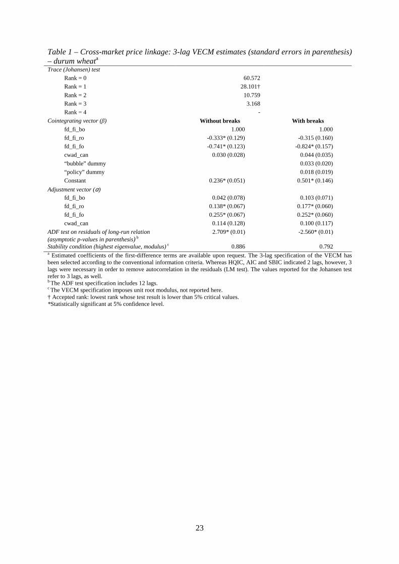
This section discusses the estimation results for the two fixed-commodity/cross-market cases,

that is, durum wheat and corn. In the case of durum wheat, the rank of the cointegration

matrix is equal to one (Table 1). Though the international (Rotterdam) price presents strong

evidence of explosive behaviour, the residuals from the cointegration relation remain

stationary and the stability condition is respected. Therefore, we can conclude that the

presence of co-explosiveness in the VECM model can be excluded. This may be attributed to

the presence of the structural breaks that may take into account the period of more intense

price turmoil though, in fact, results suggest that an explosive root can be excluded even when

structural breaks are not included in the model specification.

When no break is included, in the cointegration vector both coefficients of the national prices

(two “satellite” markets) are significant while the coefficient of the Rotterdam price is not and

is much lower than the others. When structural breaks are included, however, only the

coefficient associated to the Southern-Italian price remains statistically insignificant. With or

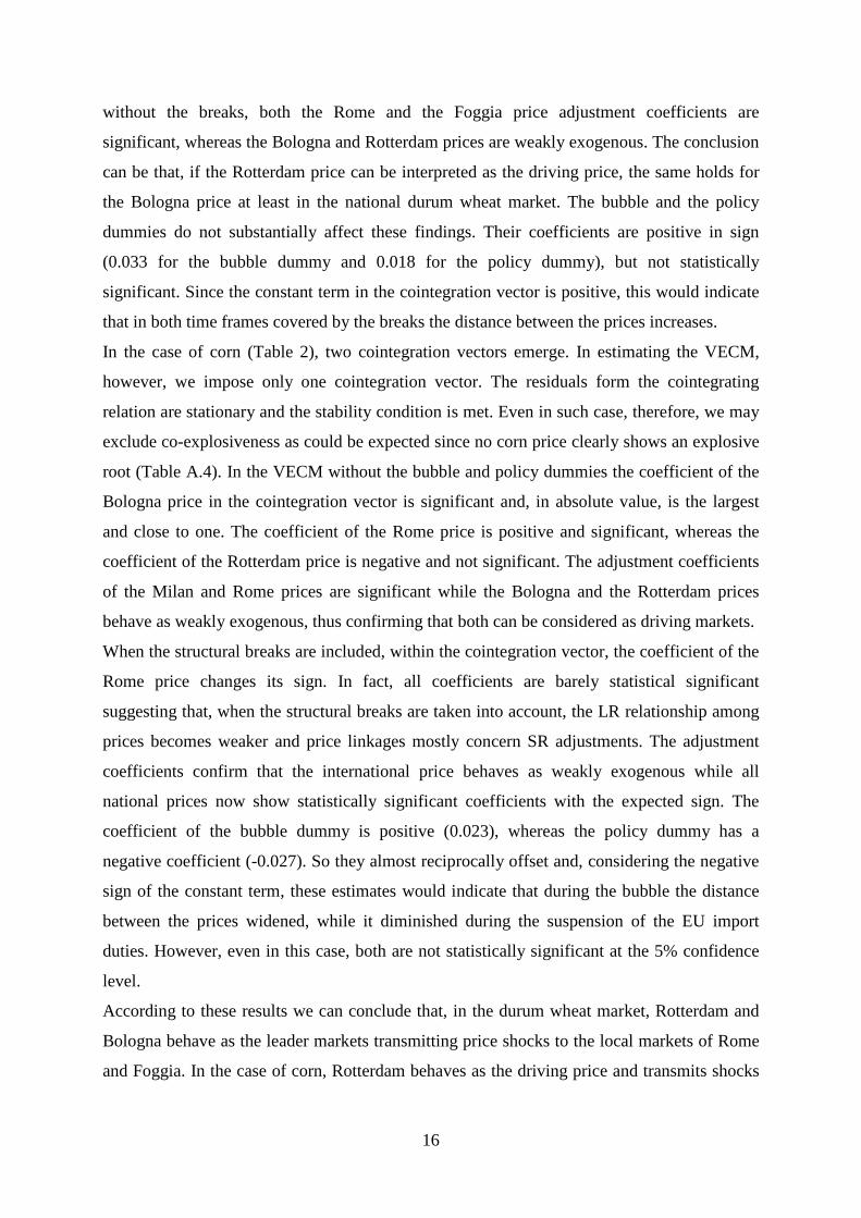
16

without the breaks, both the Rome and the Foggia price adjustment coefficients are

significant, whereas the Bologna and Rotterdam prices are weakly exogenous. The conclusion

can be that, if the Rotterdam price can be interpreted as the driving price, the same holds for

the Bologna price at least in the national durum wheat market. The bubble and the policy

dummies do not substantially affect these findings. Their coefficients are positive in sign

(0.033 for the bubble dummy and 0.018 for the policy dummy), but not statistically

significant. Since the constant term in the cointegration vector is positive, this would indicate

that in both time frames covered by the breaks the distance between the prices increases.

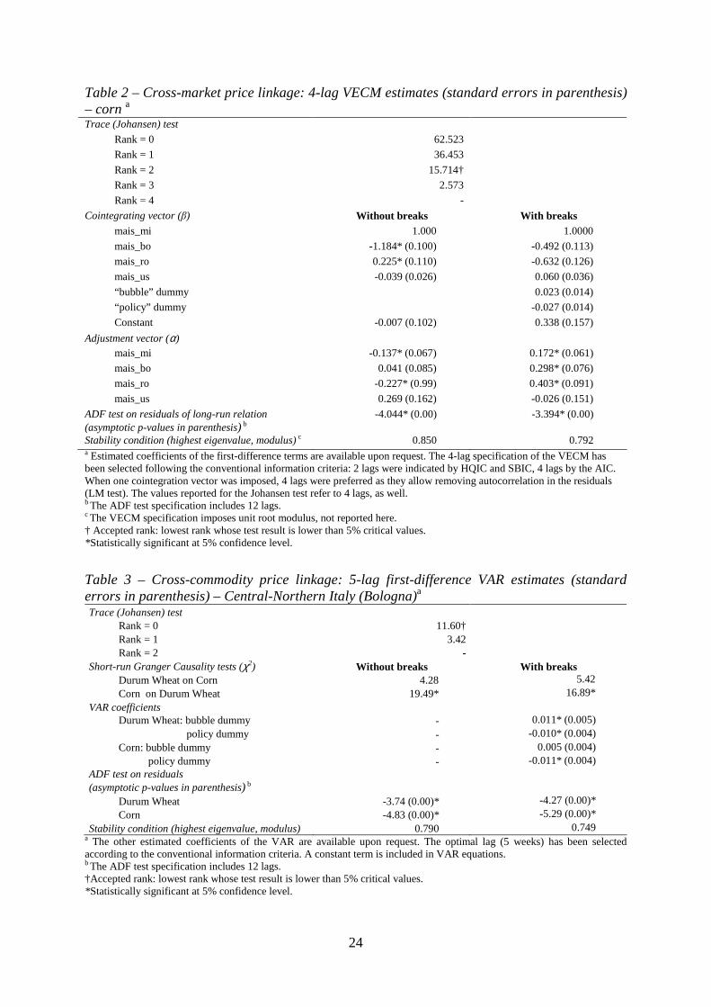
In the case of corn (Table 2), two cointegration vectors emerge. In estimating the VECM,

however, we impose only one cointegration vector. The residuals form the cointegrating

relation are stationary and the stability condition is met. Even in such case, therefore, we may

exclude co-explosiveness as could be expected since no corn price clearly shows an explosive

root (Table A.4). In the VECM without the bubble and policy dummies the coefficient of the

Bologna price in the cointegration vector is significant and, in absolute value, is the largest

and close to one. The coefficient of the Rome price is positive and significant, whereas the

coefficient of the Rotterdam price is negative and not significant. The adjustment coefficients

of the Milan and Rome prices are significant while the Bologna and the Rotterdam prices

behave as weakly exogenous, thus confirming that both can be considered as driving markets.

When the structural breaks are included, within the cointegration vector, the coefficient of the

Rome price changes its sign. In fact, all coefficients are barely statistical significant

suggesting that, when the structural breaks are taken into account, the LR relationship among

prices becomes weaker and price linkages mostly concern SR adjustments. The adjustment

coefficients confirm that the international price behaves as weakly exogenous while all

national prices now show statistically significant coefficients with the expected sign. The

coefficient of the bubble dummy is positive (0.023), whereas the policy dummy has a

negative coefficient (-0.027). So they almost reciprocally offset and, considering the negative

sign of the constant term, these estimates would indicate that during the bubble the distance

between the prices widened, while it diminished during the suspension of the EU import

duties. However, even in this case, both are not statistically significant at the 5% confidence

level.

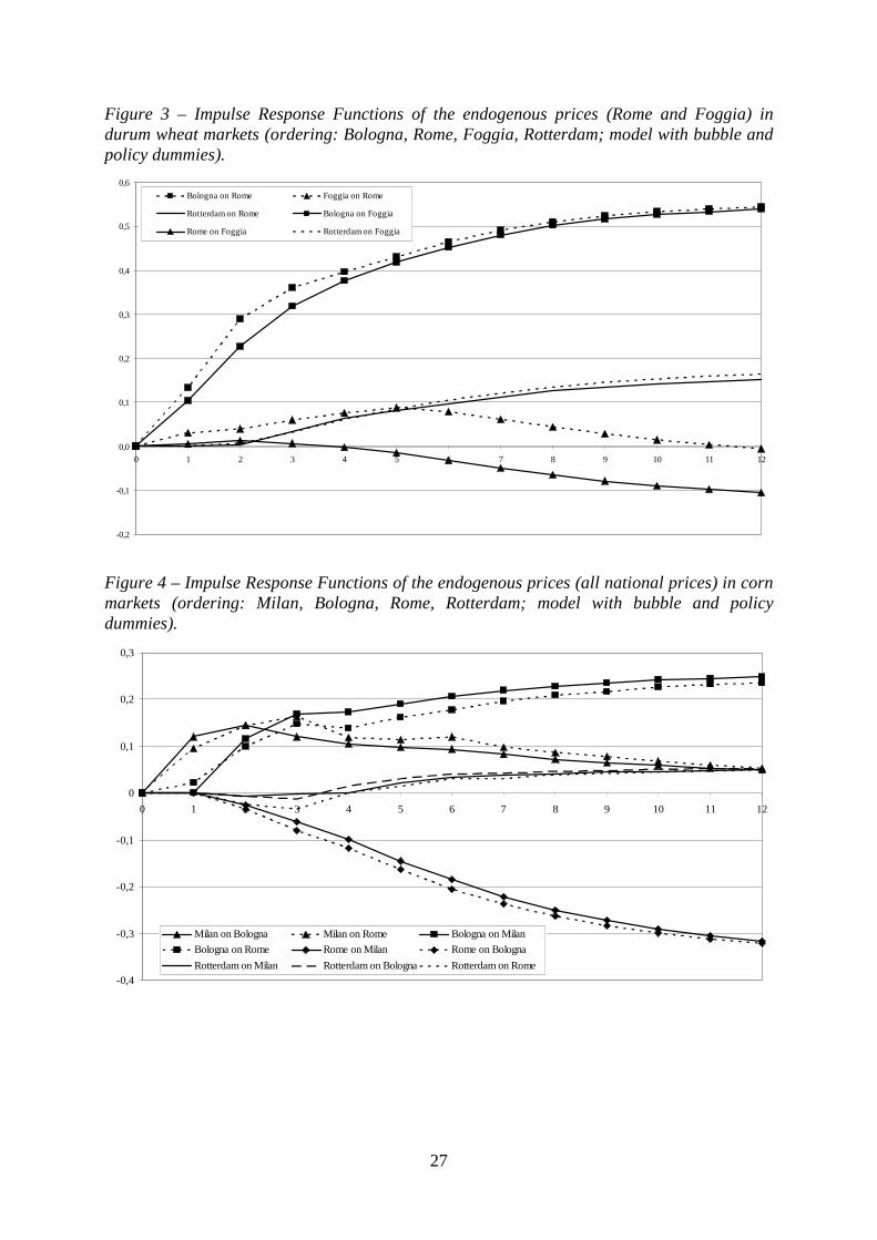
According to these results we can conclude that, in the durum wheat market, Rotterdam and

Bologna behave as the leader markets transmitting price shocks to the local markets of Rome

and Foggia. In the case of corn, Rotterdam behaves as the driving price and transmits shocks

17

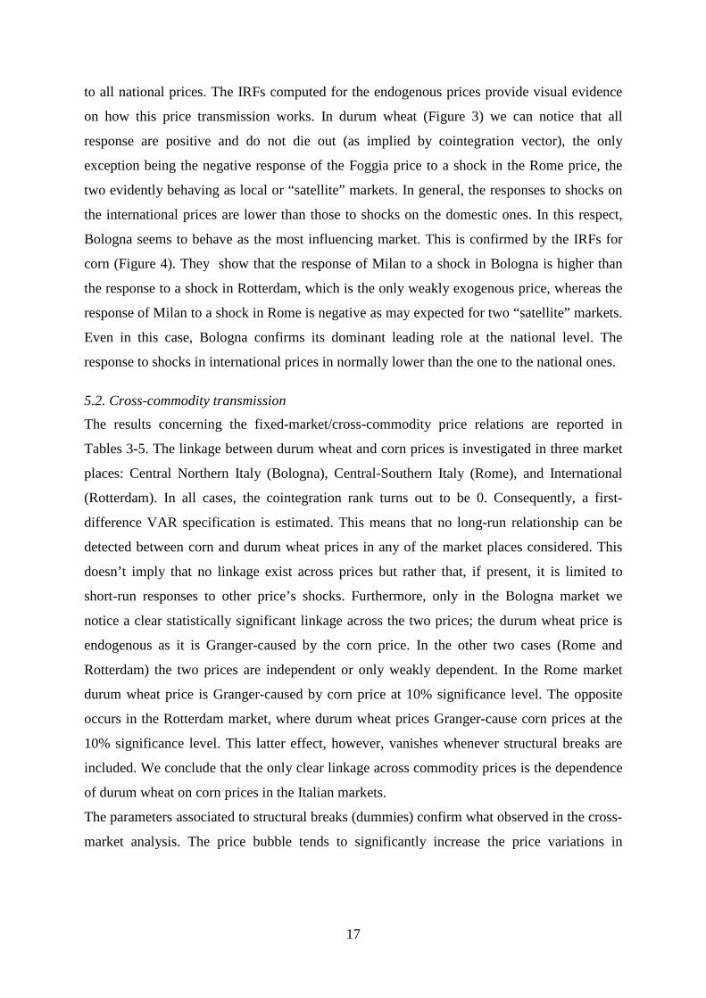
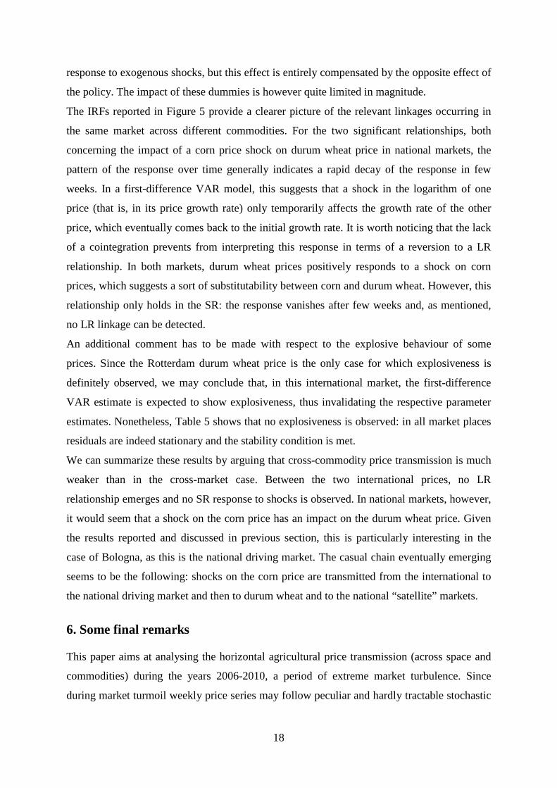
to all national prices. The IRFs computed for the endogenous prices provide visual evidence

on how this price transmission works. In durum wheat (Figure 3) we can notice that all

response are positive and do not die out (as implied by cointegration vector), the only

exception being the negative response of the Foggia price to a shock in the Rome price, the

two evidently behaving as local or “satellite” markets. In general, the responses to shocks on

the international prices are lower than those to shocks on the domestic ones. In this respect,

Bologna seems to behave as the most influencing market. This is confirmed by the IRFs for

corn (Figure 4). They show that the response of Milan to a shock in Bologna is higher than

the response to a shock in Rotterdam, which is the only weakly exogenous price, whereas the

response of Milan to a shock in Rome is negative as may expected for two “satellite” markets.

Even in this case, Bologna confirms its dominant leading role at the national level. The

response to shocks in international prices in normally lower than the one to the national ones.

5.2. Cross-commodity transmission

The results concerning the fixed-market/cross-commodity price relations are reported in

Tables 3-5. The linkage between durum wheat and corn prices is investigated in three market

places: Central Northern Italy (Bologna), Central-Southern Italy (Rome), and International

(Rotterdam). In all cases, the cointegration rank turns out to be 0. Consequently, a first-

difference VAR specification is estimated. This means that no long-run relationship can be

detected between corn and durum wheat prices in any of the market places considered. This

doesn’t imply that no linkage exist across prices but rather that, if present, it is limited to

short-run responses to other price’s shocks. Furthermore, only in the Bologna market we

notice a clear statistically significant linkage across the two prices; the durum wheat price is

endogenous as it is Granger-caused by the corn price. In the other two cases (Rome and

Rotterdam) the two prices are independent or only weakly dependent. In the Rome market

durum wheat price is Granger-caused by corn price at 10% significance level. The opposite

occurs in the Rotterdam market, where durum wheat prices Granger-cause corn prices at the

10% significance level. This latter effect, however, vanishes whenever structural breaks are

included. We conclude that the only clear linkage across commodity prices is the dependence

of durum wheat on corn prices in the Italian markets.

The parameters associated to structural breaks (dummies) confirm what observed in the cross-

market analysis. The price bubble tends to significantly increase the price variations in

18

response to exogenous shocks, but this effect is entirely compensated by the opposite effect of

the policy. The impact of these dummies is however quite limited in magnitude.

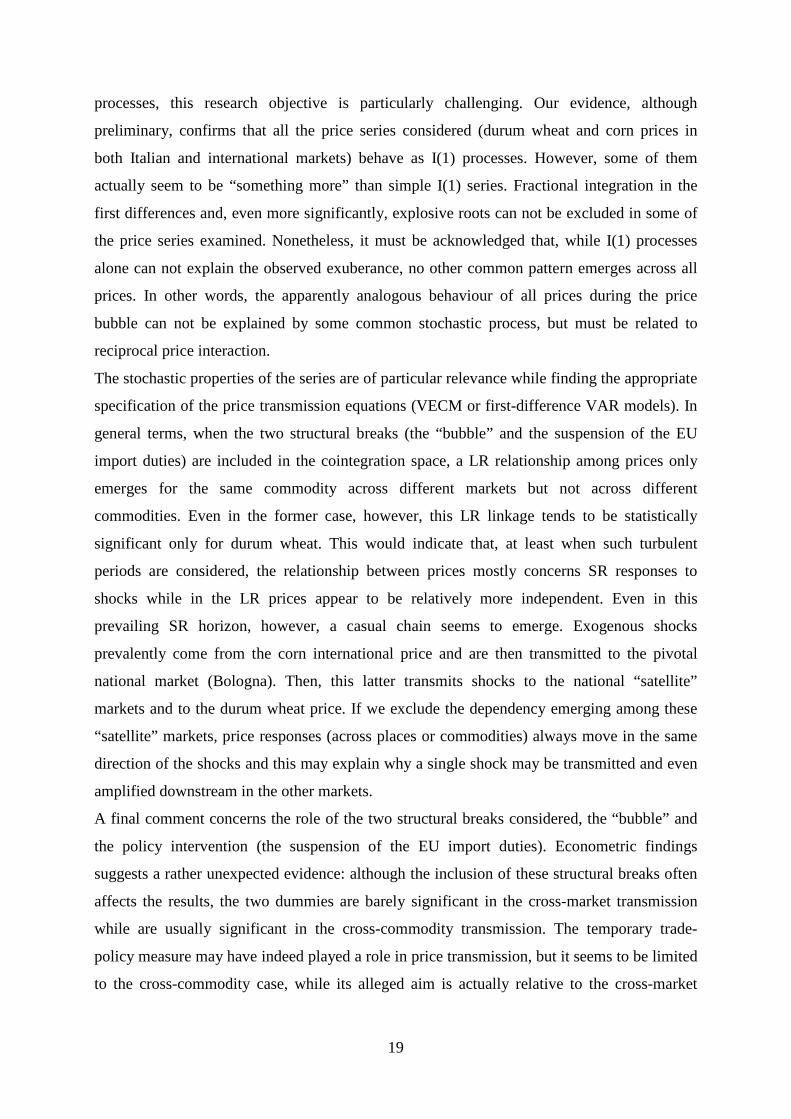
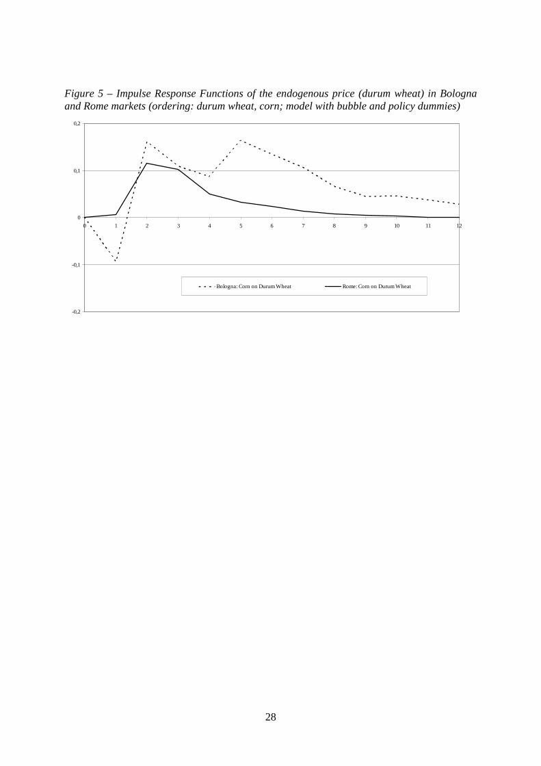
The IRFs reported in Figure 5 provide a clearer picture of the relevant linkages occurring in

the same market across different commodities. For the two significant relationships, both

concerning the impact of a corn price shock on durum wheat price in national markets, the

pattern of the response over time generally indicates a rapid decay of the response in few

weeks. In a first-difference VAR model, this suggests that a shock in the logarithm of one

price (that is, in its price growth rate) only temporarily affects the growth rate of the other

price, which eventually comes back to the initial growth rate. It is worth noticing that the lack

of a cointegration prevents from interpreting this response in terms of a reversion to a LR

relationship. In both markets, durum wheat prices positively responds to a shock on corn

prices, which suggests a sort of substitutability between corn and durum wheat. However, this

relationship only holds in the SR: the response vanishes after few weeks and, as mentioned,

no LR linkage can be detected.

An additional comment has to be made with respect to the explosive behaviour of some

prices. Since the Rotterdam durum wheat price is the only case for which explosiveness is

definitely observed, we may conclude that, in this international market, the first-difference

VAR estimate is expected to show explosiveness, thus invalidating the respective parameter

estimates. Nonetheless, Table 5 shows that no explosiveness is observed: in all market places

residuals are indeed stationary and the stability condition is met.

We can summarize these results by arguing that cross-commodity price transmission is much

weaker than in the cross-market case. Between the two international prices, no LR

relationship emerges and no SR response to shocks is observed. In national markets, however,

it would seem that a shock on the corn price has an impact on the durum wheat price. Given

the results reported and discussed in previous section, this is particularly interesting in the

case of Bologna, as this is the national driving market. The casual chain eventually emerging

seems to be the following: shocks on the corn price are transmitted from the international to

the national driving market and then to durum wheat and to the national “satellite” markets.

6. Some final remarks

This paper aims at analysing the horizontal agricultural price transmission (across space and

commodities) during the years 2006-2010, a period of extreme market turbulence. Since

during market turmoil weekly price series may follow peculiar and hardly tractable stochastic

19

processes, this research objective is particularly challenging. Our evidence, although

preliminary, confirms that all the price series considered (durum wheat and corn prices in

both Italian and international markets) behave as I(1) processes. However, some of them

actually seem to be “something more” than simple I(1) series. Fractional integration in the

first differences and, even more significantly, explosive roots can not be excluded in some of

the price series examined. Nonetheless, it must be acknowledged that, while I(1) processes

alone can not explain the observed exuberance, no other common pattern emerges across all

prices. In other words, the apparently analogous behaviour of all prices during the price

bubble can not be explained by some common stochastic process, but must be related to

reciprocal price interaction.

The stochastic properties of the series are of particular relevance while finding the appropriate

specification of the price transmission equations (VECM or first-difference VAR models). In

general terms, when the two structural breaks (the “bubble” and the suspension of the EU

import duties) are included in the cointegration space, a LR relationship among prices only

emerges for the same commodity across different markets but not across different

commodities. Even in the former case, however, this LR linkage tends to be statistically

significant only for durum wheat. This would indicate that, at least when such turbulent

periods are considered, the relationship between prices mostly concerns SR responses to

shocks while in the LR prices appear to be relatively more independent. Even in this

prevailing SR horizon, however, a casual chain seems to emerge. Exogenous shocks

prevalently come from the corn international price and are then transmitted to the pivotal

national market (Bologna). Then, this latter transmits shocks to the national “satellite”

markets and to the durum wheat price. If we exclude the dependency emerging among these

“satellite” markets, price responses (across places or commodities) always move in the same

direction of the shocks and this may explain why a single shock may be transmitted and even

amplified downstream in the other markets.

A final comment concerns the role of the two structural breaks considered, the “bubble” and

the policy intervention (the suspension of the EU import duties). Econometric findings

suggests a rather unexpected evidence: although the inclusion of these structural breaks often

affects the results, the two dummies are barely significant in the cross-market transmission

while are usually significant in the cross-commodity transmission. The temporary trade-

policy measure may have indeed played a role in price transmission, but it seems to be limited

to the cross-commodity case, while its alleged aim is actually relative to the cross-market

20

dimension. Furthermore, in all statistically significant cases the “bubble” and the policy

always operate in opposite directions. The former amplifies price variation in response to

external shocks while the latter actually reduces this response. This not only indicates that

these two structural breaks tend to reciprocally offset but also that, in fact, the policy

intervention eventually played a role in reducing the magnitude of the price response to

shocks.

21

References

Ardeni, P.G., 1989. Does the Law of One Price really hold for commodity prices? American

Journal of Agricultural Economics, 71, 661-669.

Dawson, P.J., Sanjuan, A.I., White, B., 2006. Structural breaks and the relationship between

barley and wheat future prices on the London international financial futures exchange.

Review of Agricultural Economics, 28 (4), 585-594.

Diba, B., Grossman, H., 1988. Explosive rational bubbles in stock prices. American Economic

Review, 78, 520–530.

European Commission, 2008. High prices on agricultural commodity markets: situation and

prospects. A review of causes of high prices and outlook for world agricultural markets.

European Commission, Directorate General for Agriculture and Rural Development,

Brussels, July.

Enders, W., 1995. Applied Econometric Time Series. New York: John Wiley & Sons.

Engsted, T., 2006. Explosive bubbles in the cointegrated VAR model. Finance Research

Letters, 3 (2), 154-162.

Esposti, R., Listorti, G., 2011. Agricultural Prices’ Behaviour during Market Turmoil. The

Case of the 2007-2008 Price Bubble. In: G. Cannata, C. Ievoli, C., L’agricoltura oltre le

crisi, Proceedings of the XLVII SIDEA Conference, Campobasso (Italy), September 22-25

(forthcoming).

Evans, G.W., 1991. Pitfalls in testing for explosive bubbles in asset prices. American

Economic Review, 81, 922–930.

Fackler, P. L., Goodwin, B. K., 2001. Spatial price analysis. In: B.L. Gardner, G.C. Rausser,

Handbook of Agricultural Economics. Volume 1B. Chapter 17, Amsterdam: Elsevier

Science, 972-1025.

Irwin S.H., Good D.L., 2009. Market Instability in a New Era of Corn, Soybean, and Wheat

Prices. Choices, 24 (1), 6-11.

Johansen, S., 1995. Maximum Likelihood Inference in Co-Integrated Vector Autoregressive

Processes. Oxford: Oxford University Press.

Johansen, S., Mosconi, R., Nielsen, B., 2000. Cointegration Analysis in the Presence of

Structural Breaks in the Deterministic Trend. The Econometrics Journal, 3, 216–249.

22

Listorti, G., 2007. Il ruolo delle politiche di mercato dell'UE nei meccanismi internazionali di

trasmissione dei prezzi agricoli: il caso del frumento tenero. Rivista di Economia Agraria,

LXII (2), 229-251.

Nielsen, B., 2010. Analysis of co-explosive processes. Econometric Theory, 26 (3), 882-915.

Phillips, P. C.B., 1999a. Discrete Fourier Transforms of Fractional Processes. Cowles

Foundation for Research in Economics, Discussion Paper No. 1243, Yale University.

Phillips, P.C.B., 1999b. Unit Root Log Periodogram Regression. Cowles Foundation for

Research in Economics, Discussion Paper No. 1244, Yale University.

Phillips, P., Magdalinos, T., 2009. Unit root and cointegrating limit theory when initialization

is in the infinite past. Econometric Theory, 25, 1682–1715.

Phillips, P., Wu, Y., Yu, J., 2009. Explosive behavior in the 1990s Nasdaq: When did

exuberance escalate asset values? Cowles Foundation for Research in Economics,

Discussion Paper No. 1699, Yale University.

Phillips, P., Yu, J., 2009. Dating the timeline of financial bubbles during the subprime crisis.

SMU Economics and Statistics WP series No. 18-2009, Singapore.

Stock, J. H., Watson, M.W., 2011. Introduction to Econometrics. 3rd ed., Boston: Addison–

Wesley.

Verga, G., Zuppiroli, M., 2003. Integrazione e causalità nel mercato europeo del frumento

tenero. Rivista di Economia Agraria, LVIII (3), 323-364.

Wei A., Leuthold, R.M., 1998. Long Agricultural Future Prices: ARCH, Long Memory or

Chaos Processes? OFOR Paper n. 98-03, Department of Agricultural Economics, University

of Illinois at Urbana-Champaign.

23

Table 1 – Cross-market price linkage: 3-lag VECM estimates (standard errors in parenthesis) – durum wheata Trace (Johansen) test

Rank = 0 60.572

Rank = 1 28.101†

Rank = 2 10.759

Rank = 3 3.168

Rank = 4 -

Cointegrating vector (β) Without breaks With breaks

fd_fi_bo 1.000 1.000

fd_fi_ro -0.333* (0.129) -0.315 (0.160)

fd_fi_fo -0.741* (0.123) -0.824* (0.157)

cwad_can 0.030 (0.028) 0.044 (0.035)

“bubble” dummy 0.033 (0.020)

“policy” dummy 0.018 (0.019)

Constant 0.236* (0.051) 0.501* (0.146)

Adjustment vector (α)

fd_fi_bo 0.042 (0.078) 0.103 (0.071)

fd_fi_ro 0.138* (0.067) 0.177* (0.060)

fd_fi_fo 0.255* (0.067) 0.252* (0.060)

cwad_can 0.114 (0.128) 0.100 (0.117)

ADF test on residuals of long-run relation

(asymptotic p-values in parenthesis) b 2.709* (0.01) -2.560* (0.01)

Stability condition (highest eigenvalue, modulus) c 0.886 0.792 a Estimated coefficients of the first-difference terms are available upon request. The 3-lag specification of the VECM has been selected according to the conventional information criteria. Whereas HQIC, AIC and SBIC indicated 2 lags, however, 3 lags were necessary in order to remove autocorrelation in the residuals (LM test). The values reported for the Johansen test refer to 3 lags, as well. b The ADF test specification includes 12 lags. c The VECM specification imposes unit root modulus, not reported here. † Accepted rank: lowest rank whose test result is lower than 5% critical values. *Statistically significant at 5% confidence level.

24

Table 2 – Cross-market price linkage: 4-lag VECM estimates (standard errors in parenthesis) – corn a Trace (Johansen) test

Rank = 0 62.523

Rank = 1 36.453

Rank = 2 15.714†

Rank = 3 2.573

Rank = 4 -

Cointegrating vector (β) Without breaks With breaks

mais_mi 1.000 1.0000

mais_bo -1.184* (0.100) -0.492 (0.113)

mais_ro 0.225* (0.110) -0.632 (0.126)

mais_us -0.039 (0.026) 0.060 (0.036)

“bubble” dummy 0.023 (0.014)

“policy” dummy -0.027 (0.014)

Constant -0.007 (0.102) 0.338 (0.157)

Adjustment vector (α)

mais_mi -0.137* (0.067) 0.172* (0.061)

mais_bo 0.041 (0.085) 0.298* (0.076)

mais_ro -0.227* (0.99) 0.403* (0.091)

mais_us 0.269 (0.162) -0.026 (0.151)

ADF test on residuals of long-run relation

(asymptotic p-values in parenthesis) b -4.044* (0.00) -3.394* (0.00)

Stability condition (highest eigenvalue, modulus) c 0.850 0.792 a Estimated coefficients of the first-difference terms are available upon request. The 4-lag specification of the VECM has been selected following the conventional information criteria: 2 lags were indicated by HQIC and SBIC, 4 lags by the AIC. When one cointegration vector was imposed, 4 lags were preferred as they allow removing autocorrelation in the residuals (LM test). The values reported for the Johansen test refer to 4 lags, as well. b The ADF test specification includes 12 lags. c The VECM specification imposes unit root modulus, not reported here. † Accepted rank: lowest rank whose test result is lower than 5% critical values. *Statistically significant at 5% confidence level.

Table 3 – Cross-commodity price linkage: 5-lag first-difference VAR estimates (standard errors in parenthesis) – Central-Northern Italy (Bologna)a Trace (Johansen) test

Rank = 0 11.60† Rank = 1 3.42 Rank = 2 -

Short-run Granger Causality tests (χ2) Without breaks With breaks Durum Wheat on Corn 4.28 5.42 Corn on Durum Wheat 19.49* 16.89*

VAR coefficients Durum Wheat: bubble dummy - 0.011* (0.005)

policy dummy - -0.010* (0.004) Corn: bubble dummy - 0.005 (0.004)

policy dummy - -0.011* (0.004) ADF test on residuals (asymptotic p-values in parenthesis) b

Durum Wheat -3.74 (0.00)* -4.27 (0.00)* Corn -4.83 (0.00)* -5.29 (0.00)*

Stability condition (highest eigenvalue, modulus) 0.790 0.749 a The other estimated coefficients of the VAR are available upon request. The optimal lag (5 weeks) has been selected according to the conventional information criteria. A constant term is included in VAR equations. b The ADF test specification includes 12 lags. †Accepted rank: lowest rank whose test result is lower than 5% critical values. *Statistically significant at 5% confidence level.

25

Table 4 – Cross-commodity price linkage: 3-lag first-difference VAR estimates (standard errors in parenthesis) – Central-Southern Italy (Rome) a Trace (Johansen) test

Rank = 0 16.06† Rank = 1 5.24 Rank = 2 -

Short-run Granger Causality tests (χ2) Without breaks With breaks Durum Wheat on Corn 3.63 2.39 Corn on Durum Wheat 6.23 7.83*

VAR coefficients Durum Wheat: bubble dummy - 0.014*(0.004)

policy dummy - -0.011*(0.004) Corn: bubble dummy - 0.003(0.006)

policy dummy - -0.011*(0.005) ADF test on residuals (asymptotic p-values in parenthesis) b

Durum Wheat -3.24* (0.00) -4.12* (0.00) Corn -4.56* (0.00) -4.91* (0.00)

Stability condition (highest eigenvalue, modulus) 0.714 0.553 a The other estimated coefficients of the VAR are available upon request. The optimal lag (3 weeks) has been selected according to the conventional information criteria. A constant terms in included in VAR equations. b The ADF test specification includes 12 lags. †Accepted rank: lowest rank whose test result is lower than 5% critical values. *Statistically significant at 5% confidence level.

Table 5 – Cross-commodity price linkage: first-difference VAR estimates – International markets (Rotterdam) a Trace (Johansen) test

Rank = 0 11.35† Rank = 1 3.02 Rank = 2 -

Short-run Granger Causality tests (χ2) Without breaks With breaks Durum Wheat on Corn 2.87 3.35 Corn on Durum Wheat 6.49 3.06

VAR coefficients Durum Wheat: bubble dummy - 0.016* (0.007)

policy dummy - -0.017* (0.007) Corn: bubble dummy - 0.007 (0.008)

policy dummy - -0.010 (0.007) ADF test on residuals (asymptotic p-values in parenthesis) b

Durum Wheat -3.65* (0.00) -4.61* (0.00) Corn -4.16* (0.00) -4.14* (0.00)

Stability condition (highest eigenvalue, modulus) 0.681 0.583 a The other estimated coefficients of the VAR are available upon request. The optimal lag (3 weeks) has been selected according to the conventional information criteria. A constant terms in included in VAR equations. b The ADF test specification includes 12 lags. †Accepted rank: lowest rank whose test result is lower than 5% critical values. *Statistically significant at 5% confidence level.

26

Fig

ure

1 –

Th

e p

rice b

ub

ble

: du

rum

wh

ea

t an

d co

rn p

rice se

ries o

ver th

e p

erio

d b

etw

ee

n M

ay

20

06

an

d D

ece

mb

er 2

01

0 (se

e A

nn

ex 1

for p

rice co

de

s).

0

100

200

300

400

500

600

700

800

02/05/2006

02/07/2006

02/09/2006

02/11/2006

02/01/2007

02/03/2007

02/05/2007

02/07/2007

02/09/2007

02/11/2007

02/01/2008

02/03/2008

02/05/2008

02/07/2008

02/09/2008

02/11/2008

02/01/2009

02/03/2009

02/05/2009

02/07/2009

02/09/2009

02/11/2009

02/01/2010

02/03/2010

02/05/2010

02/07/2010

02/09/2010

02/11/2010

fd_

fi_b

ofd

_fi_

fofd

_fi_

ro

cwa

d_

can

ma

is_

bo

ma

is_

mi

ma

is_

rom

ais

_u

s

€/ton

Fig

ure

2 –

Da

ting

the

bu

bb

le: tim

e se

ries o

f the

forw

ard

recu

rsive A

DF

t-statistic fo

r the

du

rum

wh

ea

t an

d co

rn p

rice se

ries (lo

ga

rithm

s) (see

An

ne

x 1 fo

r price

cod

es).

-3,0

-2,0

-1,0

0,0

1,0

2,0

3,0

27/01/2007

27/02/2007

27/03/2007

27/04/2007

27/05/2007

27/06/2007

27/07/2007

27/08/2007

27/09/2007

27/10/2007

27/11/2007

27/12/2007

27/01/2008

27/02/2008

27/03/2008

27/04/2008

27/05/2008

27/06/2008

27/07/2008

27/08/2008

27/09/2008

27/10/2008

27/11/2008

27/12/2008

27/01/2009

27/02/2009

27/03/2009

27/04/2009

27/05/2009

27/06/2009

27/07/2009

27/08/2009

27/09/2009

27/10/2009

27/11/2009

27/12/2009

27/01/2010

27/02/2010

27/03/2010

27/04/2010

27/05/2010

27/06/2010

27/07/2010

27/08/2010

27/09/2010

27/10/2010

27/11/2010

27/12/2010

1%

Critic

al V

alu

e A

DF

ma

is_

us

fd_

fi_b

o

fd_

fi_fo

fd_

fi_ro

ma

is_

bo

ma

is_

mi

ma

is_

ro

cw

ad

_c

an

Price

bu

bb

le

Su

spe

nsio

n o

f EU

imp

ort d

utie

s

27

Figure 3 – Impulse Response Functions of the endogenous prices (Rome and Foggia) in durum wheat markets (ordering: Bologna, Rome, Foggia, Rotterdam; model with bubble and policy dummies).

-0,2

-0,1

0,0

0,1

0,2

0,3

0,4

0,5

0,6

0 1 2 3 4 5 6 7 8 9 10 11 12

Bologna on Rome Foggia on Rome

Rotterdam on Rome Bologna on Foggia

Rome on Foggia Rotterdam on Foggia

Figure 4 – Impulse Response Functions of the endogenous prices (all national prices) in corn markets (ordering: Milan, Bologna, Rome, Rotterdam; model with bubble and policy dummies).

-0,4

-0,3

-0,2

-0,1

0

0,1

0,2

0,3

0 1 2 3 4 5 6 7 8 9 10 11 12

Milan on Bologna Milan on Rome Bologna on Milan

Bologna on Rome Rome on Milan Rome on Bologna

Rotterdam on Milan Rotterdam on Bologna Rotterdam on Rome

28

Figure 5 – Impulse Response Functions of the endogenous price (durum wheat) in Bologna and Rome markets (ordering: durum wheat, corn; model with bubble and policy dummies)

-0,2

-0,1

0

0,1

0,2

0 1 2 3 4 5 6 7 8 9 10 11 12

Bologna: Corn on Durum Wheat Rome: Corn on Durum Wheat

29

ANNEX 1 – Price commodities and groups under analysis

Table A.1 – Codification and description of the prices adopted in the analysis Price Code Product Description Market Place fd_fi_bo Durum Wheat, Fino Bologna (Central-Northern Italy)

fd_fi_fo Durum Wheat, Fino Foggia (Southern Italy)

fd_fi_ro Durum Wheat, Fino Rome (Central-Southern Italy)

mais_bo Maize, Ibrido Nazionale Bologna (Central-Northern Italy)

mais_mi Maize, Ibrido Nazionale Milan (Northern Italy)

mais_ro Maize, Ibrido Nazionale Rome (Central-Southern Italy)

cwad_cana Wheat, Canada Western Amber Durum (CWAD) Canada, St Lawrence/Rotterdam

mais_usa Maize, #3 Yellow Corn (3YC) US, Gulf/Rotterdam a CIF price

Table A.2 – Price groups for the analysis of price linkages (VECM or first-difference VAR models) Group of Interdependent

Commodities/Markets Property of the Series Estimated Model

Fixed Commodity-Cross Market DURUM WHEAT VECM

fd_fi_bo I(1)

fd_fi_ro I(1)

fd_fi_fo I(1)

cwad_cana I(1) + explosive root

CORN VECM

mais_mi I(1)

mais_bo I(1)

mais_ro I(1)

mais_usa I(1)

Fixed Market-Cross Commodity CENTRAL-NORTHERN ITALY (Bologna) First-difference VAR

fd_fi_bo I(1)

mais_bo I(1)

CENTRAL-SOUTHERN ITALY (Rome) First-difference VAR

fd_fi_ro I(1)

mais_ro I(1)

INTERNATIONAL (Rotterdam) First-difference VAR

cwad_cana I(1) + explosive root

mais_usa I(1) a CIF price

30

ANNEX 2 – Unit and explosive roots testing

Table A.3 – Unit root tests on ikp and ikp∆1 : Adjusted Dickey-Fuller (ADF)a, Phillips-Perron (PP) b,

Adjusted Dickey-Fuller GLS (ADF GLS)c and Kwiatkowski, Phillips, Schmidt e Shin (KPSS)d test; p-values in parenthesis; the values for which the null is rejected are in bold (10% critical values)

ikp ikp∆1 Price

ADF PP ADF GLS KPSS ADF PP ADF GLS KPSS fd_fi_bo -1.075

(0.728) -1.112 (0.710)

-1.196 (0.213)

0.368 (0.091)

-5.428 (0.000)

-6.501 (0.000)

-3.686 (0.000)

0.171 (>0.100)

fd_fi_fo -1.887 (0.339)

-1.226 (0.662)

-1.098 (0.247)

0.376 (0.088)

-2.128 (0.234)

-6.616 (0.000)

-2.446 (0.014)

0,190 (>0.100)

fd_fi_ro -1.909 (0.328)

-1.124 (0.705)

-1.330 (0.170)

0.376 (0.087)

-2.005 (0.285)

-6.218 (0.000)

-2.586 (0.009)

0.180 (>0.100)

mais_bo -1.534 (0.516)

-1.656 (0.454)

-0.298 (0.579)

0.377 (0.087)

-3.494 (0.008)

-7.619 (0.000)

-2.841 (0.004)

0.168 (>0.100)

mais_mi -1.534 (0.516)

-1.615 (0.475)

0.388 (0.544)

0.369 (0.091)

-3.545 (0.007)

-8.694 (0.000)

-1.966 (0.047)

0.175 (>0.100)

mais_ro -1.616 (0.474)

-1.815 (0.373)

-0.461 (0.516)

0,374 (0.089)

-2.704 (0.073)

-11.388 (0.000)

-2.213 (0.026)

0.155 (>0.100)

cwad_can -1.067 (0.731)

-1.374 (0.595)

-0.637 (0.442)

0.365 (0.093)

-2.831 (0.054)

-14.008 (0.000)

-2.839 (0.004)

0.242 (>0.100)

mais_us -2.234 (0.194)

-2.399 (0.142)

0.125 (0.722)

0.377 (0.087)

-2.487 (0.118)

-15.302 (0.000)

-1.703 (0.084)

0.160 (>0.100)

a H0: unit root. The test specification includes a constant term, and all significant lags “testing down” up to a maximum of 12. b H0: unit root. The test specification includes 12 lags and a constant term.

c H0: unit root. The test specification includes a constant term and all significant lags “testing down” up to a maximum of 12. d H0: no unit root. The test specification includes 12 lags and a constant term; p-values are interpolated

Table A.4 – Test of fractional integration on ikp and ikp∆1

according to Phillips (1999a,b)a and

SADF tests (forward recursive regressions) of explosive roots on ikp according to Phillips et

al.(2009)b; p-values in parenthesis; the cases for which the null is rejected are in bold (5% critical values, respectively). All test specifications with a constant term and 12 lags

Test of fractional integration

ikp ikp∆1

SADF test on ikp Price

t (H0: d=0) z (H0: d=1) t (H0: d=0) z (H0: d=1) (r=0.1) (r=0.2)

fd_fi_bo 11.359 (0.000)

1.569 (0.117)

2.367 (0.029)

-4.532 (0.000)

1.376 (>0.050)

1.376 (>0.050)

fd_fi_fo 10.410 (0.000)

1.565 (0.118)

1.567 (0.134)

-4.774 (0.000)

1.789 (<0.050)

0.888 (>0.100)

fd_fi_ro 15.347 (0.000)

1.687 (0.092)

2.728 (0.014)

-4.132 (0.000)

1.370 (>0.050)

1.154 (>0.100)

mais_bo 4.306 (0.000)

1.913 (0.056)

1.799 (0.089)

-4.343 (0.000)

7.018 (<0.010)

0.997 (>0.100)

mais_mi 4.314 (0.000)

1.741 (0.082)

2.564 (0.020)

-3.751 (0.000)

11.865 (<0.010)

1.365 (>0.050)

mais_ro 5.087 (0.000)

0.862 (0.389)

1.742 (0.100)

-4.303 (0.000)

1.339 (>0.050)

1.339 (>0.050)

cwad_can 9.765 (0.000)

1.641 (0.101)

2.081 (0.052)

-3.912 (0.000)

2.396 (<0.010)

2.396 (<0.010)

mais_us 5.484 (0.000)

0.320 (0.749)

0.671 (0.510)

-5.689 (0.000)

2.653 (<0.010)

-0.559 (>0.100)

a If d=0 the series is I(0); if d=1 the series is I(1); if 0<d<1, the series is I(d) (long memory process). As a deterministic trend has been excluded, the original test has not been detrended. The test runs under alternative possible values of the arbitrary power parameter (see Phillips, 1999a,b) here assumed equal to 0.55. Test robustness is performed using a set of values of the power parameter ranging from 0.4 to 0.75. Test results for these alternative values of the power parameter are available on request. They do not significantly differ from those presented here. b H0: no explosive root. Critical values for both sample sizes of 100 and 500 give the same test outcome.