POLITEHNICA UNIVERSITY OF BUCHAREST THE FACULTY OF COMPUTER SCIENCE AND

AUTOMATIC CONTROL

DIPLOMA PROJECT

DISTRIBUTED ALGORITHMS

FOR THE MONALISA FRAMEWORK

UPB Scientific Coordinator: Prof. Dr. Eng. Valentin CRISTEA California University of Technology Coordinator: Dr. Iosif LEGRAND

Author: Ion Bogdan BRINZAREA

2004

1

INTRODUCTION..............................................................................................................3

The MonALISA framework .......................................................................................................................................3

Vision and Goals for JINI ...........................................................................................................................................3

System Components ......................................................................................................................................................7

Infrastructure Component ..........................................................................................................................................8

Programming Model Component .............................................................................................................................9

Services Component......................................................................................................................................................9

Interaction and Interdependence between Components ....................................................................................9

System Service Architecture.....................................................................................................................................10

The MonALISA service architecture .....................................................................................................................12

The monitoring service...............................................................................................................................................13

The data collection engine .........................................................................................................................................14

Data storage...................................................................................................................................................................15

Registration and Discovery.......................................................................................................................................16

Predicates, Filters and Alarm Agents ....................................................................................................................17

The VRVS system........................................................................................................................................................18

Dynamic routing ..........................................................................................................................................................19

The existing approach ................................................................................................................................................20

Contribution..................................................................................................................................................................22

A HIGHLY ASYNCHRONOUS MINIMUM SPANNING TREE...............................24

Introduction ..................................................................................................................................................................24

Problem formulation...................................................................................................................................................24

Basic concepts ...............................................................................................................................................................25

The pioneering work of Gallager, Humblet and Spira [1] ...............................................................................26

An improvement in node counting from Chin, Ting [3] ...................................................................................29

An optimal algorithm by Awerbuch [4] ................................................................................................................29

2

Corectness of previous algorithms ..........................................................................................................................31

A minimum spanning tree protocol ........................................................................................................................33

The composite protocol ..............................................................................................................................................34

DISTRIBUTED DELAY CONSTRAINED MULTICAST PATH SETUP ALGORITHM FOR HIGH SPEED NETWORKS.......................................................37

Steiner problem in graphs .........................................................................................................................................37

Problem For mulation .................................................................................................................................................38

Algorithm.......................................................................................................................................................................38

A GENETIC ALGORITHM FOR STEINER TREE OPTIMIZATION WITH MULTIPLE CONSTRAINTS USING PRÜFER NUMBER.......................................42

Introduction ..................................................................................................................................................................42

Problem formulation...................................................................................................................................................43

Genetic algorithms ......................................................................................................................................................44

Genotype: modified Prufer numbers .....................................................................................................................44

The pre-processing phase..........................................................................................................................................45

The initial population .................................................................................................................................................46

The fitness function.....................................................................................................................................................47

Selection..........................................................................................................................................................................47

Crossover .......................................................................................................................................................................48

Mutation .........................................................................................................................................................................49

IMPLEMENTATION.......................................................................................................50

CONCLUSIONS.............................................................................................................58

REFERENCES ...............................................................................................................59

APPENDIX......................................................................................................................61

3

Introduction

The MonALISA framework

The MonALISA (Monitoring Agents in A Large Integrated Services Architecture) system provides a distributed monitoring service. MonALISA is based on a scalable Dynamic Distributed Services Architecture (DDSA), which is designed to meet the needs of physics collaborations for monitoring global Grid systems, and is implemented using JINI/JAVA and WSDL/SOAP technologies. The scalability of the system derives from the use of multithreaded Station Servers to host a variety of loosely coupled self-describing dynamic services, the ability of each service to register itself and then to be discovered and used by any other services, or clients that require such information, and the ability of all services and clients subscribing to a set of events (state changes) in the system to be notified automatically. The framework integrates several existing monitoring tools and procedures to collect parameters describing computational nodes, applications and network performance. It has built- in SNMP support and network-performance monitoring algorithms that enable it to monitor end-to-end network performance as well as the performance and state of site facilities in a Grid. MonALISA is currently running around the clock on the US CMS test Grid as well as an increasing number of other sites. It is also being used to monitor the performance and optimize the interconnections among the reflectors in the VRVS system.

Vision and Goals for JINI

The JINI architecture consists of a core infrastructure component, a programming model, and service components that collaborate to provide a dynamic, distributed, self-healing network where services can discover and join spontaneously. It is a Java-based solution and can be considered as a network extension of the core Java application model. It is a simple, elegant solution for the complex dynamic distributed computing problem.

As a dynamic distributed technology, JINI has the following vision and goals:

• To provide an infrastructure to connect anything, anytime, anywhere. The vision of JINI is to provide an infrastructure that can help different network users to discover, join, and participate in any network community spontaneously.

• To provide an infrastructure to enable "network plug and work." The goal of JINI is to make any service joining the network available for other users without installation and configuration hassles. The vision is 0% installation and 0% configuration. It should be as easy as plugging a telephone into a telephone jack and using it—but it is not there yet. In fact, today's services are more operating system-and driver-centric. Even after downloading appropriate drivers and appropriate configuring, it is more a scenario of "plug and pray" than of "plug and play."

4

• To support a service-based architecture by abstracting the hardware/software distinction. JINI's vision is to provide an architecture centered around a service network instead of a computer network or device network. JINI's architecture simplifies the pervasive nature of computing by treating everything as a service. This service can be provided through hardware, software, or a combination of both. The advantage in abstracting this way enables the infrastructure to be designed to accommodate a single type of entity—a service. All protocols, such as joining or leaving the network, can be defined with respect to this service type instead of individual types. Such abstraction also helps in hiding the implementation of the service provider from the service requester.

• To provide an architecture to handle partial failure. A distributed architecture is not complete until it provides a mechanism for handling partial failures. JINI's vision is to provide an infrastructure and an associated programming model that can handle partial failures and help in establishing a self-healing network of services.

JINI's architecture is based on the following environmental assumptions

• The existence of a network with reasonable network latency This is to ensure that network latency does not affect the performance of a JINI system because JINI relies heavily on Java's mobile-code feature.

• Each JINI-enabled device has some memory and processing power. For devices without processing power or memory, a proxy exists that contains both processing power and memory. This is a strong assumption because all network citizens are expected to have minimum computing capability, memory, and ability to communicate.

• Each device should be equipped with a Java Virtual Machine (JVM). The availability of different JVM footprints makes it easier to Java-enable any device.

• Service components are implemented using Java. This is an assumption for software components that would be joining a JINI community. All the service components should live as Java objects to facilitate the service requester to download and run code dynamically. The point to note here is that JINI does not expect a Java service implementation but a Java wrapper.

The only assumption, which is very strong, is the expectation of JINI-enabled devices. These are devices with minimum computing capabilities, communicating capabilities, and memory that should host a Java Virtual Machine (JVM). This is fine for many devices, but it can cause problems for the numerous devices that are currently processor-less and driver-controlled. But the provision of a proxy (any device that has a processor, memory, and network capability willing to represent a processor- less device) makes this assumption easier to meet. By this approach, you can use a desktop computer to represent all your processor- less devices, such as printers, scanners, electric switches, washing machines, and microwave ovens, and also to control them.

5

The JINI architecture consists of the following components

• An infrastructure component, which enables building a federation of JVM

• A programming model component, which provides a set of interfaces for constructing reliable distributed services

6

• The services component, which forms the living entities and represents the offered functionality within the federation

Although the system has three component parts, the boundary between the parts is blurred. All three parts collaborate with each other, like a set of gears within a machine, to achieve the overall system objectives. In fact, the infrastructure and the services components are built using the programming model component interfaces.

JINI architecture is a Java-based solution for dynamic distributed computing. The JINI system extends the Java application environment from a single JVM to a network of JVMs. From that perspective, JINI can be seen as a network extension of the infrastructure, programming model, and services of Java application environment. JINI utilizes most of the core Java technologies, such as RMI and JavaBeans, while adding additional functionality to meet the distributed/network nature of the system.

7

Regarding the question: “How tightly are JINI architecture and Java coupled? “, the answer has two parts:

• JINI is tightly coupled with Java as an application environment and a programming model.

• JINI is not coupled with Java as a language.

This means that the service can be implemented in any language: C, C++, or JPython. But to participate in the architecture, it should be subjected to a compiler that can produce Java-compliant byte code. If not, it can be Java wrapped/Java-tized using Java native interface (JNI). In this way, even a legacy application can be Java-wrapped and can be made into a JINI service. To summarize: JINI architecture is not Java language-centric but Java application-centric.

System Components

The JINI system comprises three components: (1) the infrastructure, (2) a programming model, and (3) services.

8

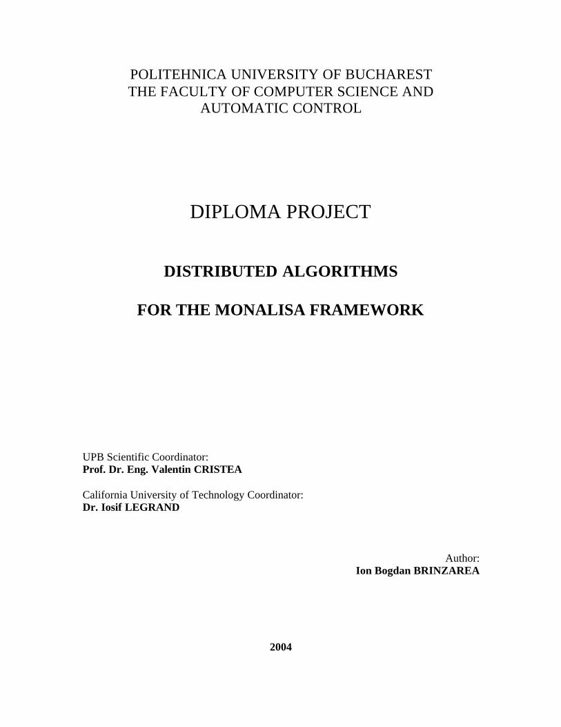
Infrastructure Component

The Infrastructure component is a core part of the architecture and its goal is to provide mechanisms for devices, services, and users to discover, join, and detach from the network. The Infrastructure component is composed of the following subcomponents:

• Discovery and join protocol, which defines the way that services discover, become part of, and advertise services to the other members of the federation.

• Remote method invocation (RMI), the distributed architecture environment that enables service proxies to be downloaded.

• Distributed security model, which provides the concept of security within the network. The distributed security model is an extension of Java's security model for distributed systems.

• Lookup service, which serves as a repository of services and helps network members to find each other within the JINI community. Entries in the repository are Java-compliant byte-code objects, which can be written in Java or wrapped by Java.

9

Programming Model Component

The programming model is based on the Java application platform and its ability to move code between nodes. The programming model defines a set of interfaces, which taken together become the distributed extension of the Java programming model to form the JINI programming model. The programming model supports the following interfaces:

• Lease interface, which extends the Java programming model by adding time to the notion of holding a reference. This approach provides a renewable, duration-based model for allocating and freeing the resource references.

• Event notification interface, which extends the popular JavaBeans component event delegation model. This model allows an event to be handled by third-party objects and recognizes that the delivery of the distributed notification may be delayed.

• Transaction interface, which allows the system to handle object-oriented transaction handling. The interface does not define the actual mechanisms involved in the transaction but provides rules for the objects involved in the transaction. This approach provides freedom in choosing the preferred mechanics and individual object implementation.

Services Component

The services component represents an important concept within JINI architecture, and it denotes the entities that have come together to form the JINI community. The entities could be hardware, software, or a combination of hardware and software. The services are identified as Java objects within the system. Each service has an interface, which defines the operations that can be requested of that service. The interface also reflects the service type. A service is a composite entity and can be composed of other subservices. In fact, the lookup service—one of the subcomponents of the core JINI infrastructure—is implemented as a JINI service. Other constituents that form a part of JINI architecture and implemented as JINI services are:

• JavaSpaces service, which provides an optional distributed persistence mechanism for the objects within a JINI community

• Transaction manager service, which provides distributed transactions for the distributed objects

Interaction and Interdependence between Components

As stated above, although the system has three parts, each part has a specific role in the overall architecture and they work in tandem to achieve the overall system objective.

10

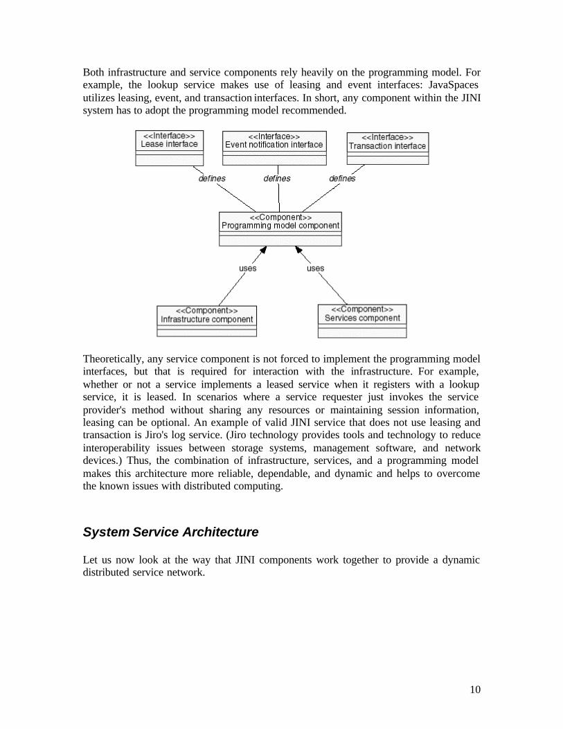
Both infrastructure and service components rely heavily on the programming model. For example, the lookup service makes use of leasing and event interfaces: JavaSpaces utilizes leasing, event, and transaction interfaces. In short, any component within the JINI system has to adopt the programming model recommended.

Theoretically, any service component is not forced to implement the programming model interfaces, but that is required for interaction with the infrastructure. For example, whether or not a service implements a leased service when it registers with a lookup service, it is leased. In scenarios where a service requester just invokes the service provider's method without sharing any resources or maintaining session information, leasing can be optional. An example of valid JINI service that does not use leasing and transaction is Jiro's log service. (Jiro technology provides tools and technology to reduce interoperability issues between storage systems, management software, and network devices.) Thus, the combination of infrastructure, services, and a programming model makes this architecture more reliable, dependable, and dynamic and helps to overcome the known issues with distributed computing.

System Service Architecture

Let us now look at the way that JINI components work together to provide a dynamic distributed service network.

11

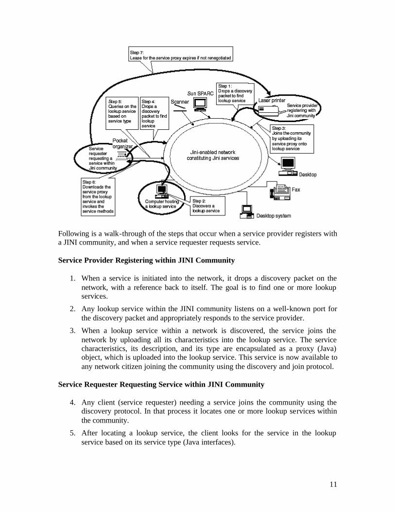
Following is a walk-through of the steps that occur when a service provider registers with a JINI community, and when a service requester requests service.

Service Provider Registering within JINI Community

1. When a service is initiated into the network, it drops a discovery packet on the network, with a reference back to itself. The goal is to find one or more lookup services.

2. Any lookup service within the JINI community listens on a well-known port for the discovery packet and appropriately responds to the service provider.

3. When a lookup service within a network is discovered, the service joins the network by uploading all its characteristics into the lookup service. The service characteristics, its description, and its type are encapsulated as a proxy (Java) object, which is uploaded into the lookup service. This service is now available to any network citizen joining the community using the discovery and join protocol.

Service Requester Requesting Service within JINI Community

4. Any client (service requester) needing a service joins the community using the discovery protocol. In that process it locates one or more lookup services within the community.

5. After locating a lookup service, the client looks for the service in the lookup service based on its service type (Java interfaces).

12

6. Once the service is found, the client invokes the service, which involves moving the proxy code on to the client. Now the client can perform any operation on the service by calling its methods. This movement of the code between the lookup service and the client gives the service provider greater freedom in the communication pattern and makes it possible to maintain the integrity of the proxy code as it is supplied by the service provider.

7. Once the service proxy is downloaded, a service requester, depending upon its requirements, creates, negotiates, or terminates its lease with the service provider.

The MonALISA service architecture

The DDSA architecture incorporates many features that make it suitable for managing and optimizing workflow through Data Grids composed of hundreds of sites, with thousands of computing and storage elements, and thousands of pending tasks, such as those foreseen by the LHC experiments. In order to scale and operate robustly in managing global, resource-constrained Grid systems, the DDSA framework uses a set of Station Servers, one per facility or site in a Grid, that host a variety of dynamic, agent-based services. The services are registered with, and can be mutually discovered by a lookup service, and they are notified automatically in case of ``events'' signaling a change of state anywhere in a large distributed system. This allows the ensemble of services to cooperate in real time to gather, disseminate, and process time-dependent state and configuration information about the site facilities, networks, and many jobs running throughout the Grid. The monitored information is reported to higher level services, that in turn analyze the information, and take corrective action to improve the overall efficiency of operation of the Grid (through load balancing, for example) or to mitigate problems as needed. The DDSA framework is inherently distributed, ``loosely coupled'' and self-restarting, making it scalable and robust. Cooperating services and applications are able to access each other seamlessly, to adapt rapidly to a dynamic environment (such as worldwide-distributed analysis by hundreds of physicists in a major HEP experiment). The services are managed by an efficient multithreading engine that schedules and oversees their execution, such that Grid operations are not disrupted if one or more tasks (threads) are unable to inaccessibility of multiple Grid components (when a key network link goes down, for example). A service in the DDSA framework is a component that interacts autonomously with other services through dynamic proxies or agents that use self-describing protocols. By using dedicated lookup services, a distributed services registry, and the discovery and notification mechanisms, the services are able to access each other seamlessly. The use of dynamic remote event subscription allows a service to register to be notified of a selected set of event types, even if there is no provider to do the notification at registration time. The lookup discovery service will then automatically notify all the subscribed services, when a new service, or a new service attribute, becomes available.

13

The code mobility paradigm (mobile agents or dynamic proxies) used in the DDSA extends the remote procedure call and the client server approach. Both the code and the appropriate parameters are downloaded dynamically into the system. Several advantages of this paradigm are: optimized asynchronous communication and disconnected operation, remote interaction and adaptability, dynamic parallel execution and autonomous mobility. The combination of the DDSA service features and code mobility makes it possible build an extensible hierarchy of services capable of managing very large Grids, with relatively little program code. A prototype implementation of the DDSA based on JINI technology was developed. The JINI architecture federates groups of devices and software components into a single, dynamic distributed system; functionality that the future Open Grid Services Architecture (OGSA) will need to include. JINI enables services to find each other on a network and allows these services to participate and cooperate within certain types of operations, while interacting autonomously with clients or other services. This architecture simplifies the construction, operation and administration of complex systems by:

• allowing registered services to interact in a dynamic and robust (multithreaded) way;

• allowing the system to adapt when devices or services are added or removed, with no user intervention;

• providing mechanisms for services to register and describe themselves, so that services can intercommunicate and use other services without prior knowledge of the services' detailed implementation.

WSDL/SOAP, bindings for all the distributed objects were also included, in order to provide access to the monitoring information from other types of clients and to facilitate a possible future migration to the Open Grid Services Architecture.

The monitoring service

An essential part of managing a global Data Grid is a monitoring system that is able to monitor and track the many site facilities, networks, and the many tasks in progress, in real time. The monitoring information gathered also is essential for developing the required higher level services, and components of the Grid system that provide decision support, and eventually some degree of automated decisions, to help maintain and optimize workflow through the Grid. We therefore developed the agent-based MonALISA system, based on the DDSA framework. MonALISA is an ensemble of autonomous multi- threaded, self-describing agent-based subsystems which are registered as dynamic services and are able to collaborate and cooperate in performing a wide range of monitoring tasks in large scale distributed applications, and to be discovered and used by other services or clients that require such information.

14

MonALISA is designed to easily integrate existing monitoring tools and procedures and to provide this information in a dynamic, self describing way to any other services or clients. MonALISA services are organized in groups and this attribute is used for registration and discovery.

The data collection engine

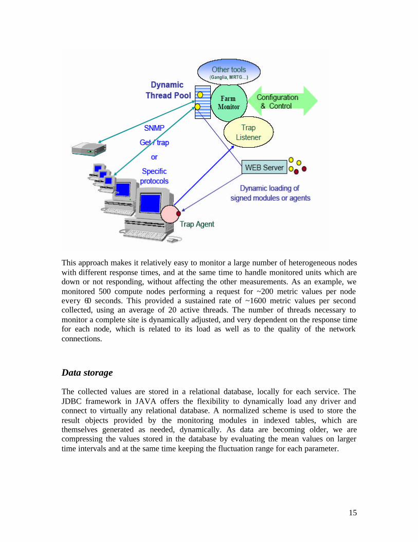
The system monitors and tracks site computing farms and network links, routers and switches using SNMP, and it dynamically loads modules that make it capable of interfacing existing monitoring applications and tools (e.g. Ganglia, MRTG, Hawkeye). The core of the monitoring service is based on a multithreaded system used to perform the many data collection tasks in parallel, independently. The modules used for collecting different sets of information, or interfacing with other monitoring tools, are dynamically loaded and executed in independent threads. In order to reduce the load on systems running MonALISA, a dynamic pool of threads is created once, and the threads are then reused when a task assigned to a thread is completed. This allows one to run concurrently and independently a large number of monitoring modules, and to dynamically adapt to the load and the response time of the components in the system. If a monitoring task fails or hangs due to I/O errors, the other tasks are not delayed or disrupted, since they are executing in other, independent threads. A dedicated control thread is used to stop properly the threads in case of I/O errors, and to reschedule those tasks that have not been successfully completed. A priority queue is used for the tasks that need to be performed periodically. A schematic view of this mechanism of collecting data is shown in figure below.

15

This approach makes it relatively easy to monitor a large number of heterogeneous nodes with different response times, and at the same time to handle monitored units which are down or not responding, without affecting the other measurements. As an example, we monitored 500 compute nodes performing a request for ~200 metric values per node every 60 seconds. This provided a sustained rate of ~1600 metric values per second collected, using an average of 20 active threads. The number of threads necessary to monitor a complete site is dynamically adjusted, and very dependent on the response time for each node, which is related to its load as well as to the quality of the network connections.

Data storage

The collected values are stored in a relational database, locally for each service. The JDBC framework in JAVA offers the flexibility to dynamically load any driver and connect to virtually any relational database. A normalized scheme is used to store the result objects provided by the monitoring modules in indexed tables, which are themselves generated as needed, dynamically. As data are becoming older, we are compressing the values stored in the database by evaluating the mean values on larger time intervals and at the same time keeping the fluctuation range for each parameter.

16

Registration and Discovery

Each MonALISA service registers with a set of JINI Lookup Discovery Services (LUS) as part of a group, and having a set of attributes. The LUSs are also JINI services and each one may be registered with the other LUSs. If two LUSs have common groups any information related with a change of state detected for a service in the common group by one is replicated to the other one. In this way it is possible to build a distributed and reliable network for registration of services and this technology allows dynamically

adding or removing LUSs from the system. Any service should also provide for registration the code base for the proxies that other services or clients need to instantiate for using it. This approach is used to make sure that the right proxies are used for each service while different versions may be used in a distributed organization at the same time. The registration is based on a lease mechanism that is responsible to verify periodically that each service is alive. In case a service fails to renew its lease, it is removed from the LUSs and a notification is sent to all the services or clients that subscribed for such events.

17

Any monitor client services is using the Lookup Discovery Services to find all the active MonALISA services running as part of one or several group “communities”. It is possible to select the services based on a set of matching attributes. The discovery mechanism is used for notification when new services are started or when services are no longer available. The communication between interested services or clients is based on a remote event notification mechanism that also supports subscription. The client application connects directly with each service it is interested in for receiving monitoring information. To perform this operation, it first downloads the proxies for the service it is interested in from a list of possible URLs specified as an attribute of each service, and than it instantiate the necessary classes to communicate with the service. This procedure allows each service to correctly interact with other services.

Predicates, Filters and Alarm Agents

The clients can get any real- time or historical data by using a predicate mechanism for requesting or subscribing to selected measured values. These predicates are based on regular expressions to match the attribute description of the measured values a client is interested in. They may also be used to impose additional conditions or constraints for selecting the values. In case of requests for historical data, the predicates are used to generate SQL queries into the local database. The subscription will create a dedicated thread to serve each client. This thread will perform the matching test for all the predicates submitted by a client with the measured values in the data flow. The same thread is responsible to send the selected results back to the client as compressed serialized objects. Having an independent thread per client allows sending the information they need, fast, in a reliable way and it is not affected by communication errors that may occur with other clients. In case of communication problems these threads will try to reestablish the connection or to cleanup the subscriptions for a client or a service that is not anymore active. Monitoring data requests with the predicate mechanism is also possible using the WSDL/SOAP binding from clients or services written in other languages. The class description for predicates and the methods to be used are described in WSDL and any client can create dynamically and instantiate the objects it needs for communication. Currently, the Web Services technology does not provide the functionality to register as a listener and to receive the future measurements a client may want to receive. Other applications or clients may also use the Agent Filters to receive the information they need. The Agent Filter is a java module which can be dynamically deployed to any MonALISA service, and is designed to perform a dedicated data processing task on local data (by subscribing with a predicate to the data flow) and returns back the processed information periodically. The MonALISA service provides the run time environment for these agents that must be digitally signed by a trusted certificate. As an example, such filters are used to compute the aggregate IO traffic in a farm, or to provide the number of

18

nodes that are free. The same thread used for handling the predicate subscription is used for sending the filtered results back to each client. Dynamically loadable alarm agents, and agents able to take actions when abnormal behavior is detected, were developed to help with managing and improving the working efficiency of the facilities, and the overall Grid system being monitored.

The VRVS system

The Virtual Rooms VideoConferencing System (VRVS) is an enhanced web based video conferencing system that is using a set of reflectors distributed world wide for an efficient real-time distribution of the audio and video streams. For each VRVS reflector, a MonALISA service is running using an embedded database, for storing the results locally, and runs in a mode that aims to minimize the reflector resources it uses (typically less than 16MB of memory and practically without affecting the system load). Dedicated modules to interact with the VRVS reflectors were developed: to collect information about the topology of the system; to monitor and track the traffic among the reflectors and report communication errors with the peers; and to track the number of clients and active virtual rooms. In addition, overall system information is monitored and reported in real time for each reflector: such as the load, CPU usage, and total traffic in and out. A dedicated GUI for the VRVS version was developed as a java web-start client. This GUI provides real time information dynamically for all the reflectors which are

19

monitored. If a new reflector is started it will automatically appear in the GUI and its connections to its peers will be shown. Filter agents to compute an exponentially mediated quality factor of each connection are dynamically deployed to every MonALISA service, and they report this information to all active clients who are subscribed to receive this information.

It provides real-time information about the way the VRVS system is used (number of conferences or clients) the topological connectivity of the reflectors and the quality of it and system related information (IO traffic CPU load). Clients can also get historical data for any of these parameters. The subscription mechanism allows one to monitor in real time any measured parameter in the system as all the updates are dynamically displayed on the open windows. Examples of some of the services and information available, visualizing the number of clients and the active virtual rooms, the traffic in and out of all the reflectors, as well as problems such as lost packets between reflectors. In addition to dedicated monitoring modules and filters for the VRVS system, we developed agents able to supervise the running of the VRVS reflectors automatically. This will be particularly important when scaling up the VRVS system further. In case a VRVS reflector stops or does not answer correctly to the monitoring requests, the agent will try to restart it. If this operation fails twice the Agent will send an email to a list of administrators. These agents are the first generation of modules capable of reacting and taking well defined actions when errors occur in the system. These agents, capable to take action in the system, may be dynamically loaded. For security reasons such agents must be digitally signed by developers with trusted certificates, declared for each running service.

Dynamic routing

Agents able to provide an optimized dynamic routing of the videoconferencing data streams were developed. These agents require information about the quality of the alternative connections in the system and they solve, in real- time, a minimum spanning tree problem to optimize the data flow at the global level. To evaluate the connection quality with possible peer reflectors monitoring agents performing ping like measurements using UDP packages were developed and they are deployed on all the MonALISA services. These agents perform continuously (every 2s) such measurements with a selected set of possible peers, which can be dynamically reconfigured, for each reflector. We are using small UDP packages to evaluate the Round Trip Time (RTT), its jitter and the percentage of lost packages.

20

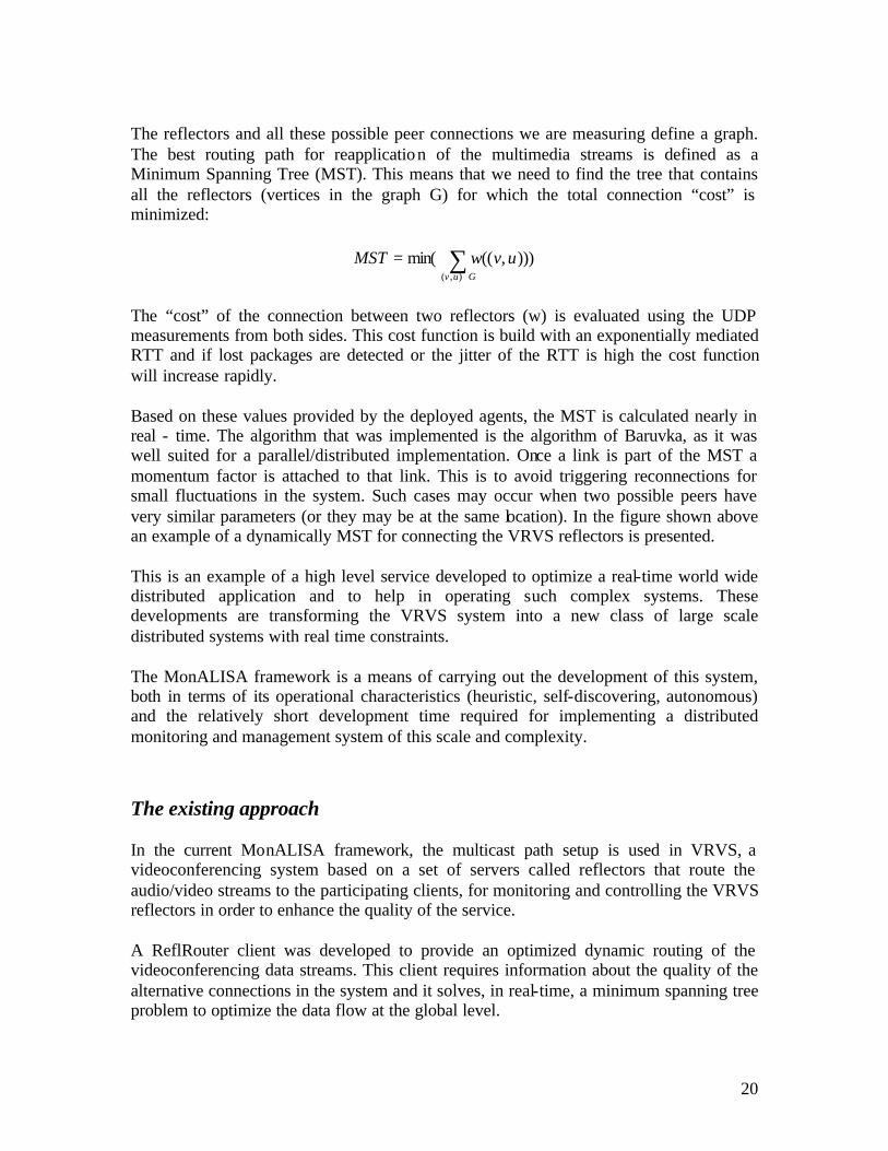
The reflectors and all these possible peer connections we are measuring define a graph. The best routing path for reapplication of the multimedia streams is defined as a Minimum Spanning Tree (MST). This means that we need to find the tree that contains all the reflectors (vertices in the graph G) for which the total connection “cost” is minimized:

))),((min(),(

∑∈

=Guv

uvwMST

The “cost” of the connection between two reflectors (w) is evaluated using the UDP measurements from both sides. This cost function is build with an exponentially mediated RTT and if lost packages are detected or the jitter of the RTT is high the cost function will increase rapidly. Based on these values provided by the deployed agents, the MST is calculated nearly in real - time. The algorithm that was implemented is the algorithm of Baruvka, as it was well suited for a parallel/distributed implementation. Once a link is part of the MST a momentum factor is attached to that link. This is to avoid triggering reconnections for small fluctuations in the system. Such cases may occur when two possible peers have very similar parameters (or they may be at the same location). In the figure shown above an example of a dynamically MST for connecting the VRVS reflectors is presented. This is an example of a high level service developed to optimize a real-time world wide distributed application and to help in operating such complex systems. These developments are transforming the VRVS system into a new class of large scale distributed systems with real time constraints. The MonALISA framework is a means of carrying out the development of this system, both in terms of its operational characteristics (heuristic, self-discovering, autonomous) and the relatively short development time required for implementing a distributed monitoring and management system of this scale and complexity.

The existing approach

In the current MonALISA framework, the multicast path setup is used in VRVS, a videoconferencing system based on a set of servers called reflectors that route the audio/video streams to the participating clients, for monitoring and controlling the VRVS reflectors in order to enhance the quality of the service. A ReflRouter client was developed to provide an optimized dynamic routing of the videoconferencing data streams. This client requires information about the quality of the alternative connections in the system and it solves, in real-time, a minimum spanning tree problem to optimize the data flow at the global level.

21

To evaluate the connection quality with possible peer reflectors there were developed monitoring agents performing ping like measurements using UDP packages, which are deployed on all the MonALISA services. These agents perform continuously (every 4s) such measurements and with a selected set of possible peers, which can be dynamically reconfigured, for each reflector. The best routing path for reapplication of the multimedia streams is defined as a Minimum Spanning Tree (MST). This means that we need to find the tree that contains all the reflectors (vertices in the graph G) for which the total connection “cost” is minimized. The “cost” of the connection between two reflectors (w) is evaluated using the UDP measurements from both sides. This cost function is build with an exponentially mediated RTT and if lost packages are detected or the jitter of the RTT is high the cost function will increase rapidly. Based on these values provided by the deployed agents, the MST is calculated nearly in real - time. There are some critical cases that must be analyzed before running the MST algorithm. For this, each ReflNode is checked. If a node isn’t active then it must not appear in the MST. Further, the tunnels that start from the inactive node must also not be present in the computed tree. Therefore, the next state will be set to MUST_DEACTIVATE. If the node is active, then each link to the other reflectors (either active peers or neighbor reflectors) is checked. If the peer reflector isn’t active the respective tunnel must not be active. Another problem arises when between two reflectors there is no ABPing information, or there is only one ABPing link. In this case, the state of the both peer links depends on the current status of the peer link. If there is at least one peer link, then both must be activated. If none is active, then no peer link must be active. For the other cases the next state of a tunnel is initialized as INACTIVE, and the MST algorithm will set it as needed. For implementation, the Boruvka’s algorithm was used, as it is also appropiate for a parallel implementation. The original Borvuka algorithm is:

Given G = (V,E) T = graph consisting of V with no edges while T has < n-1 edges do

for each connected component C of T do e = min cost edge (v,u) s.t. v in C and u not in C T := T union {e}

But there can be a problem if the graph isn’t connex. In this case, there is no way to connect n-1 edges, so that condition is modified such that the while cycle repeats as long as there is at least one union made into the for cycle. In our case, while joining subtrees, we also mark the next state of each tunnel that is used to perform the respective joint as ACTIVE. Another modification that must be done to this algorithm is that the process is going to be running iterative, i.e. we compute the MST, issue commands to change the tree, then we compute the MST and change the tree again and so on. A problem that could appear is that of active links oscillation.

22

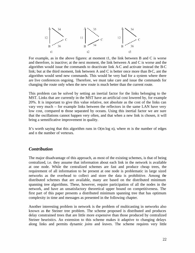
For example, as in the above figures: at moment t1, the link between B and C is worse and therefore, is inactive; at the next moment, the link between A and C is worse and the algorithm would issue the commands to deactivate link A-C and activate instead the B-C link; but at the third moment, link between A and C is better once more than B-C, ant the algorithm would send new commands. This would be very bad for a system where there are live conferences ongoing. Therefore, we must take care and issue the commands for changing the route only when the new route is much better than the current route. This problem can be solved by setting an inertial factor for the links belonging to the MST. Links that are currently in the MST have an artificial cost lowered by, for example 20%. It is important to give this value relative, not absolute as the cost of the links can vary very much – for example links between the reflectors in the same LAN have very low cost, compared to those separated by oceans. Using this inertial factor we are sure that the oscillations cannot happen very often, and that when a new link is chosen, it will bring a semnificative improvement in quality. It’s worth saying that this algorithm runs in O(m log n), where m is the number of edges and n the number of vertexes.

Contribution

The major disadvantage of this approach, as most of the existing schemes, is that of being centralized, i.e. they assume that information about each link in the network is available at one node. While the centralized schemes are fast and produce cheap trees, the requirement of all information to be present at one node is problematic in large sized networks as the overhead to collect and store the data is prohibitive. Among the distributed schemes that are available, many are based on the distributed minimum spanning tree algorithms. These, however, require participation of all the nodes in the network, and have an unsatisfactory theoretical upper bound on competitiveness. The first part of this paper presents a distributed minimum spanning tree that has optimum complexity in time and messages as presented in the following chapter. Another interesting problem in network is the problem of multicasting in networks also known as the Steiner tree problem. The scheme proposed is distributed and produces delay constrained trees that are little more expensive than those produced by centralized Steiner heuristics. An extension to this scheme makes it adaptive to changing delays along links and permits dynamic joins and leaves. The scheme requires very little

23

information in addition to that which is already maintained in routing tables for current protocols.

24

A highly asynchronous minimum spanning tree

Introduction In this chapter we present a distributed protocol for obtaining a minimum spanning tree in an asynchronous network. We assume that each edge has a distinct weight associated with it. When the protocol terminates, each node knows which edges incident on it are in the minimum spanning tree. This protocol maintains a spanning forest of trees (referred to as fragments), each of which is a subtree of the MST. Fragments are merged over their minimum weight outgoing edges until a single fragment that spans the entire network remains. In order to keep the message complexity low, each fragment has a level number associated with it which is a mesure of the number of nodes in the fragment. We present a protocol, CompMST, which requires O(min (N, (D+d) log N) time and O(E+N log N/log log N) messages where D is the maximum degree of a node and d is the diameter of the MST. To arrive at this protocol we first present a protocol Async. In Async, a fragment does not wait for another fragment to reach a particular level before it can combine with it. The protocol takes at most O(min(N,(D+d)log N) time and O(N2) messages. The features of Async and those from the [3] are combined to obtain CompMST. The requirement of balanced growth is relaxed and a fragment at level l has to wait for a neighbour fragment to reach a level greater or equal to l – log l before combining with it.The CompMST protocol behaves like the protocol in [3] when the fragment size is small and like Async when the fragment size reaches N/log N.

Problem formulation

The network is modeled like an undirected graph with N nodes and E edges. All nodes are assumed to have distinct identities. We assume that all the edges e have distinct weights w(e) and each process knows the weight of all edges incident on it. The nodes communicate via messages. Messages are not lost and they arrive at their destination within finite but unpredictable time. Further, messages sent over an edge arrive in the order in which they are sent. On the initiation of the protocol, we assume that each process knows the weight of each edge incident on it. On the termination of the protocol, each node knows which edges incident on it belong to the minimum spanning tree.

25

Basic concepts

The pioneering work presented in [1] forms the backbone of the papers in [2], [3] and [4]. In all these papers their algorithms use the following concepts: Fragments As mentioned before, the algorithm uses fragments which are connected

subgraphs of the MST Edge labels There are three possible labels for edges. Initially all the edges are

Unlabeled Thereafter, adjacent fragments join to form larger fragments by labeling their intermediate edge as Branch of the MST. Any edges that are found to connect nodes of the same fragment are labeled as Rejected, and are subsequently ignored. Each edge is labeled once in the Greedy Joining Policy described below the edges being labeled as Branch or Rejected

Outgoing edge An edge is characterized as outgoing of a fragment if one adjacent node is

in the fragment and the other is not. Fragment ID Each fragment has a unique ID identifying the fragment Level concept In addition to a unique identifier referred as Fid each fragment is

characterized by a level L. All nodes have zero level in the beginning. The level increases when two fragments join. The joining of two fragments on their common minimum outgoing edge (MOE) is referred as equi-join which differs from submission which refers to a fragments being absorbed by another fragment. Each level estimates the size of a fragment

Greedy Joining Policy Each fragment tries to find its minimum outgoing edge and joins

along another fragment. That edge is labeled Branch of the new fragment and thus an edge of the MST. Smaller fragments can submit anytime to greater ones, but greater fragments must wait on their MOE until the other fragment submits or becomes equal or greater level.

PROPERTY 1. Given a fragment of an MST, let e be a minimum-weight outgoing edge of the fragment. Then joining e and its adjacent nonfragment node to the fragment yields another fragment of an MST. PROOF. Suppose the added edge e is not in the MST containing the original fragment. Then there is a cycle formed by e and some subset of the MST edges. At least one edge x ≠ e of this cycle is also an outgoing edge of the fragment, so that w(x)≥ w(e). Thus, deleting x from the MST and adding e forms a new spanning tree which must be minimal if the original tree was minimal. The original fragment with e added is a fragment of the new MST. PROPERTY 2. If all the edges of a connected graph have different weights, then the MST is unique.

26

PROOF. Suppose, to the contrary, that there are two different MSTs. Let e be the minimum-weight edge that is in one but not both of the trees, and let T be the set of edges of the MST containing e and T' be the edge set of the other MST. The edge set {e} U T' must contain a cycle, and at least one edge of this cycle, say e', is not in T (since T contains no cycles). Since the edge weights are all different and e' is in one but not both of the trees, w(e) < w(e'). Thus {e} U T' - (e'} is the edge set of a spanning tree of smaller weight than T', yielding a contradiction. The protocol maintains a forest of rooted trees (referred to as fragments). The root of the fragment is the root of the corresponding tree and the root’s identity is used to identify the fragment. The best edge of a fragment is the minimum weight edge among all edges leading out of the fragment. The Prim-Dijkstra algorithm starts with a single node and successively enlarges the fragment until it spans the graph. The Kruskal algorithm starts with all nodes as fragments and successively extends the fragment with the smallest-weight minimum outgoing edge, combining fragments were possible. Each fragment has a level number associated with it. Fragments containing only a single node are at level 0. When two fragments at level l merge, a new fragment at level l+1 is created. For such a level numbering scheme, it can be shown that a fragment with the level number l contains at least 2l nodes. Therefore, the level number of a fragment cannot exceed log N. The level of a node is the level number of the fragment to which it belongs.

The pioneering work of Gallager, Humblet and Spira [1]

One of the major innovations of this paper, which is regarded as classic not only for the MST problem but for distributed algorithms in general, was the concept of the level. Levels characterize fragments and enforce a hierarchy, that breaks the symmetry problem in the behavior of fragments during the joining procedure. The underlying idea is that levels are an estimate of the size of the fragment. Since each level increase requires an equi­join, the maximum possible level is log(N ), which will help estimating the complexity of the algorithm. Within each fragment, one node is the root of the fragment. In their work the idea of core edge was used. The core edge is the edge on which two fragments join. The two adjacent nodes act like a root. to the edge. The other papers use the idea of root as described here. The way the root is determined will be explained later in this section. We use distance from the root to define a hierarchy (typical “father­child” hierarchy for trees). The nodes know if a message, sent along the Branches, travels from or towards the root. Naturally, the father of a node is the neighbor node towards the root. We will see that, as the root changes the father relations may change. Nodes can be roots, leaders or simple nodes.

27

• root The root is the coordinator and decision maker of its fragment. Its responsabilities are to oversee a Finding procedure and, after the completion of the Reporting procedure, to either nominate a new node (named the leader, see below) to carry out the next join, or else end the algorithm.

• leader. It is the node that attempts to join its fragment with another adjacent fragment. Its responsibilities, after having completed those of a simple node, are to follow the Joining policy and join correctly with the other fragment (this will become clear later). When the leader receives an initiate message, it becomes a simple node.

• simple node. None of the above. Its responsibilities are to participate in both the Finding procedure (find its local MOE which as we said is a MOE adjacent to this node) and the Report procedure, i.e., report the best MOE among all those reports from nodes below it in the ``father­child'' hierarchy.

It is better to examine the algorithm in all its various cases, through the explanation of the messages exchanged between nodes. We can distinguish two procedures. Finding Procedure This is the procedure by which the fragment looks for its next MOE. When a node becomes a root it starts this procedure by sending a copy of the following message over each of its Branch edges and broadcasting the following message(s).

• initiate message: The root of the fragment has mandated a search for the MOE of its fragment. The message must be forwarded along each outbound branch in the “father­child” hierarchy, thereby reaching all nodes of the fragment. It also carries the information of the new fragment identity and level.

Once a node a of fragment Fa has received such an initiate message, it must choose from its edges, the minimum outgoing one, which we will refer to as its local MOE. It picks its minimum weight Unlabeled edge and carries out the following dialog to determine where it leads to. Assume that it connects to node b of Fb .

• test message: node a asks “Is this an outgoing edge, to a greater or equal level fragment?”.

• reject message: node b can reply “No, we are in the same fragment and I have already rejected this edge myself”. It is not difficult to see that we can reject an edge using only two messages ­ even two test messages can be enough. Node a will repeat the same procedure with its next minimum Unlabeled edge, until an accept message is received (see below) or it runs out of Unlabeled edges. In this case, infinity is considered to be the weight of the local MOE.

• accept message: node b can reply “Yes, it is outgoing, and my level is greater or equal to your level”. This edge is the local MOE of the node, and the search stops.

28

However, if Lb<La , node b puts the test message aside and carries on with the procedures initiated within its own fragment. (This is case 1 where a non­trivial delay can occur in responding to a message in this algorithm.) Eventually, node b will receive an initiate message with Lb = L a , in which case it can send a delayed accept message back to node a. The only exception is if node b receives a changeRoot message in order to join along the edge (a,b) while Lb < La . In this case, node b first submits to node a and then, after the joining procedure is complete, sends a delayed reject message back to node a. In addition, since Fb joined Fa before node a reported its local MOE, node a will extend the Finding procedure into Fb .

• report message: it is the answer to the initiate message. Every node reports the

weight of its MOE to its parent. Every parent compares the incoming report messages and its local MOE and reports only the minimum of them all.

Joining Procedure The root accumulates the report messages, decides which one is the MOE for the whole fragment, and then informs the adjacent node that it will be the new leader.

• changeRoot message: it is sent along the path from the root to the node adjacent to the fragment MOE inviting that node to become the leader of the fragment. On the way the message, reverses the “father” relation of adjacent nodes and so when it finally reaches the leader, the branches of the fragment are rooted towards the leader.

Let us assume that the old root chose a as leader. Having received a changeRoot message node a knows that it can proceed in joining along the edge (a,b), which is both the local MOE of a and the MOE of the whole fragment.

• connect message: node a says “My fragment and I would like to join with you”. The joining could be either equi­join or submission. Node a, waits for a connect message (case 2 of non trivial delay) that will establish the joining in terms of equi­join (La = Lb ) or submission (La = Lb ). Note that a connect message will always lead to a join, since the only way for rejection of the edge would be if Fb submits to Fa , but this is impossible because the accept message, previously sent by b, guarantees that Lb = La . Although Lb may have increased, it could never decrease and thus the Joining Policy is not violated. This way cycles are avoided (see the correctness section).

We can now discuss the way the root is determined. In the beginning, every node is a trivial fragment and thus a root. In an equi­join, the root can be one of the two nodes adjacent to the MOE by say smaller node id number. In a submission, the root of Fb remains and node a will have b as its father. The algorithm terminates when the final root can not find an outgoing edge, i.e., the reported MOE is equal to infinity.

29

An improvement in node counting from Chin, Ting [3]

The major innovation of the algorithm is that it tries to keep the fragment level a better estimate of the fragment size. It is obvious that any fragment of level L must have at least 2L nodes. However, this is just a lower bound of its size: the fragment may have many more nodes than 2L if it has accepted a lot of submissions. The modified algorithm demands that

2L = Size(F ) = 2L+1 Tracking the fragment size can be achieved by having the root count the report messages it receives. More accurately, each report message has a counter that is increased at each hop of the message. Each node adds the counters of all the messages that it receives. At the root, the level of the fragment is compared with the size. If Size(F) = 2L+1 then the level is increased until it satisfies the previous double inequality. Then an initiate message is broadcasted and the procedure of finding the MOE is repeated. We will call this procedure Root Level Increase. A complementary idea suggested in this algorithm concerns a change in the Joining policy in order to exploit better the counting procedure. When a fragment (F1,L1) with v1 as new root, submits to (F2,L2) at node v2 with L1 < L2 , F1 will either be included in the size counting procedure of F2 or it will begin a size counting procedure for itself. Node v1 will calculate the new possible size according to the previous formula. If the new level of F1 is greater than L2 then the submission is cancelled and a new Finding procedure is initiated in F1. This procedure increases the efficiency of the algorithm to ))(( NGN ⋅Θ where G is the function explained in the introduction. Intuitively, we can observe that the mentality of the Joining Policy expects small size fragments to submit to bigger ones. By keeping in fragments, the level closely related to the size, we make the enforcement of this policy easier.

An optimal algorithm by Awerbuch [4]

This is the first algorithm that achieved the optimal bounds for both communication and time. The price paid is the loss of simplicity; two phases are required and the second one is further subdivided in two parts. Two new procedures are introduced: the Root Update procedure and the Test Distance procedure. The Root Update resembles the Root Level Increase procedure of the previous algorithm. The difference is that instead of counting the number of report messages, the existence of “long” paths is detected. The initiate message has a counter and counts the number of nodes it visits. The counter is initialised to 2L+1 and is decreased at each hop. When the counter becomes negative (we will say that the message expired), a message is sent back

30

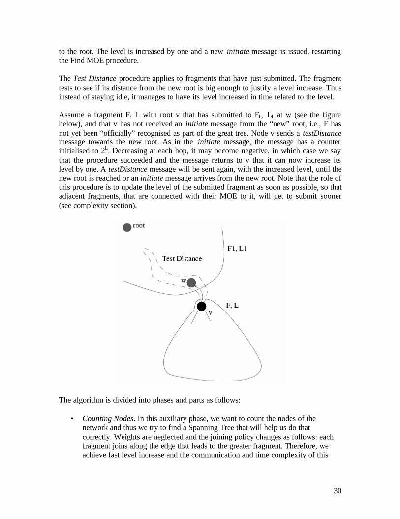
to the root. The level is increased by one and a new initiate message is issued, restarting the Find MOE procedure. The Test Distance procedure applies to fragments that have just submitted. The fragment tests to see if its distance from the new root is big enough to justify a level increase. Thus instead of staying idle, it manages to have its level increased in time related to the level. Assume a fragment F, L with root v that has submitted to F1, L1 at w (see the figure below), and that v has not received an initiate message from the “new” root, i.e., F has not yet been “officially” recognised as part of the great tree. Node v sends a testDistance message towards the new root. As in the initiate message, the message has a counter initialised to 2L. Decreasing at each hop, it may become negative, in which case we say that the procedure succeeded and the message returns to v that it can now increase its level by one. A testDistance message will be sent again, with the increased level, until the new root is reached or an initiate message arrives from the new root. Note that the role of this procedure is to update the level of the submitted fragment as soon as possible, so that adjacent fragments, that are connected with their MOE to it, will get to submit sooner (see complexity section).

The algorithm is divided into phases and parts as follows:

• Counting Nodes. In this auxiliary phase, we want to count the nodes of the network and thus we try to find a Spanning Tree that will help us do that correctly. Weights are neglected and the joining policy changes as follows: each fragment joins along the edge that leads to the greater fragment. Therefore, we achieve fast level increase and the communication and time complexity of this

31

phase are O(E +N log(N)) and O(N) respectively (see [4] for details). Having a Spanning Tree, the number of nodes in the network can be counted.

• MST phase. This is the main part of the algorithm, where an MST is found. This

phase is divided into two parts.

o Fragments' Size: 0 toN

Nlog

. In this part, the algorithm behaves exactly

the same as the first algorithm we examined. The complexity of this part is optimal (see [4] for details), because the phase ends when the sizes of the

fragments becomeN

Nlog

. Intuitively, we can observe that the first level

increases are very fast compared to the later ones.

o Fragments' Size: N

Nlog

to N . After the size of F becomes Size(F) =

NN

log, the two new procedures are brought into action. Having fragments

of this size makes sure that we have fewer than log(N) fragments in this phase.

Corectness of previous algorithms In order to prove that the algorithms are correct, we have to prove that they terminate and find the MST. For termination, the following theorem holds for the three algorithms and proves that they terminate. Theorem

The algorithms [1], [3] and [4] are deadlock free. PROOF A slightly different proof than the one in [1] will be given here. To prove that the algorithms find the minimum of the spanning trees we can recall two properties that we mentioned in the introduction. In other words it is sufficient to verify that the algorithms find at each step the MOE of each fragment. The previous description must have left no doubt that the edge selected by the root as MOE is indeed of minimum weight and outgoing for all the nodes that received the initate message and participated in the Finding procedure.

32

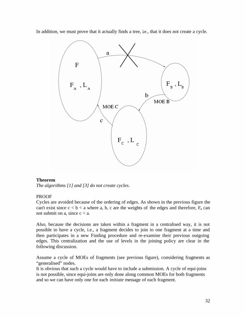
In addition, we must prove that it actually finds a tree, i.e., that it does not create a cycle.

Theorem The algorithms [1] and [3] do not create cycles. PROOF Cycles are avoided because of the ordering of edges. As shown in the previous figure the can't exist since c < b < a where a, b, c are the weights of the edges and therefore, Fa can not submit on a, since c < a. Also, because the decisions are taken within a fragment in a centralised way, it is not possible to have a cycle, i.e., a fragment decides to join to one fragment at a time and then participates in a new Finding procedure and re­examine their previous outgoing edges. This centralization and the use of levels in the joining policy are clear in the following discussion. Assume a cycle of MOEs of fragments (see previous figure), considering fragments as “generalised” nodes. It is obvious that such a cycle would have to include a submission. A cycle of equi­joins is not possible, since equi­joins are only done along common MOEs for both fragments and so we can have only one for each initiate message of each fragment.

33

After the new initiate message arrives, the level is increased. Assuming a submission, say Fc to Fa , we have to assume a difference in levels La > LC . Assume that FB wants to join with FC , then it must be LB = LC . Obviously, LA > LB and thus FA can neither submit nor equi­join with FB . This way, cycles can not be created.

A minimum spanning tree protocol

In this section we describe the Async protocol. Each iteration is executed in two phases. In the first phase, the fragment identity is propagated to all sites in the fragment. After this phase is over, the root initiates the second phase for finding the best edge. First-phase The root of a fragment initiates the first phase by sending an initiate1 message with the fragment identity (which is the identity of the root) as a parameter to its children. On receiving the message initiate1 a node updates its fragment identity and propagates initiate1 to its children. When the initiate1 message reaches a leaf node, it sends a finish message to its parent. An intermediate site waits for a finish message from all children before sending a finish message to its parent. When the root receives the finish message from all children, it knows that all nodes in the fragment know the current fragment identity. The root initiates the second phase. Second phase The root of a fragment initiates the second phase by sending initiate2 to its children. In this phase the best edge of the fragment is found as in [1]. A node sends a test message over an edge to ascertain that the edge is outgoing. However, the reply to a test message is not delayed (because if the receiving node is in the same fragment, then it must know the correct fragment identity since the first phase of the iteration has completed). After a node has determined its local best edge it propagates this edge weight towards the root using report messages. The root picks the edge with the minimum weight among the local best edges and sends a change-root message to the node in the fragment with this as an incident edge. This node becomes the new root of the fragment and sends a connect message over the best edge in an attempt to combine with the fragment at the other end. Consider the case when a connect message from a site i in fragment F reaches a site j, which is in fragment G. We have the following cases:

• if j receives initiate1 and has not sent a finish message, then j treats (i,j) as an edge of the fragment and sends initiate1 to i. Further, site j waits for a finish message from i before sending its finish message. In this case, nodes in F are absorbed in G as a part of the current iteration of G

• if j has already sent its finish message then the response to the connect message is delayed. If (i,j) is also the best edge of G then G will also send a connect message over this edge and F and G will merge ending the iteration. The node with the larger identity among the two end-points of the best edge will become the new root of the combined fragment and will initiate the next iteration. Otherwise when

34

j gets initiate1 message during the first phase of the next iteration, it will send an initiate1 message to i and as a result F will be absorbed as a part of that iteration.

Hence, fragments are absorbed only while a site is executing the first phase and no new sites are added to a fragment while in the second phase.

The composite protocol

CompMST behaves like the protocol in [3] when the fragment size is small and like Async when the fragment size becomes large. In contrast to Async, the level numbers are explicitly stored by the sites and we require that the response to a test message sent by a node i at a level l to a node j to be delayed only if the level number of j is less than l-log l. Since log l increases with l, the protocol becomes more asynchronous as l increases. In CompMST the level number of a fragment is proportional to the amount of time it has to wait before updating its level number. The changes required to Async to obtain this behaviour are explained in the following: First-Phase The initiator site sends initiate1 message to its children with its current level number and the fragment identity. On receiving initiate1 a site updates its level number and fragment identity and propagates initiate1 to its children. The number of nodes are counted while propagating the finish(count) messages, where count is the number of nodes in the subtree rooted at the node sending the message. A leaf sends a finish(1) message to its parent. After site i has received a finish(countm) message from each child m, it sums up the counts received from the children, adds one to it and sends the resulting number in a finish message to its parent. The first phase terminates after the initiator receives a finish message from each child. Let M be the sum of the counts received from the children by the initiator. The initiator then updates its level number to log(M+1). This may be greater than the level number previously stored in the initiator due to fragments absorbed during this first phase. Second Phase is modified as follows. The initiator propagates its new level number in the initiate2 messages and sites update their level numbers on receiving this message. The level number of a node is included in the test message sent by it. If a node j receives a test message from a node with level l and j’s fragment identity differs from the one received then the response is delayed by j until its level number becomes at least l-log l. In addition, we use a protocol Update which allows a node to update the level number and fragment identity of the nodes in its fragment. The initiator site starts the protocol by sending the update message to its children with the fragment identity and level number in it. On receiving update(level,id), site i updates its level number and fragment identity and propagate the update message to its children. Consider the case in which there is a sequence of fragments, F1, F2,…, Fm, all at level li such that the connect message of Fi arrives at a node in Fi+1.

35

If the best edge of Fm leads to a node in a fragment with a higher level number lj then the level numbers of nodes in F1, F2,…, Fm are updated to lj as in [1]. This updating may take

up toil

m

ii SF =∑

=1

time. This is a problem since we want a node that waits O(Sli) time

before it updates its level number to be able to increase its level number to at least liSlog and it may be the case that liSlog > lj. For this purpose we have to count the nodes in C and update the level number accordingly. The changes required in the protocol are explained in the following. Consider the case when a connect message from i in fragment F at level li is received by a node j in fragment G at level lj. If j has already sent a connect message to i (so that both F and G have the same best edge) then F and G are merged. If j>i then j becomes the root of the combined fragment and initiates a new iteration. Otherwise, i becomes the new root. If j has not sent a connect message to i then j behaves as follows:

• li > lj In this case, site j delays response to the connect message until its level becomes at least li (the connect message is then handled as described in case 2 below) or it sends a connect message to i (in this case the fragments are merged as described above)

• li <= lj a. Site j has received the initiate1 and has not sent the finish message: In this case site j propagates initiate1 to i and waits for a finish message from i before sending a finish message to its parent. Thus F is absorbed in G and nodes in F participate in the current iteration of the protocol in G). The number of nodes in F are therefore inceluded in updating the number of G. b. Site j has sent the finish message and li < lj – log lj In this case since j has already sent the finish message, the nodes in F will not be included in updating the level number of G. Therefore, we require that i counts the number of nodes in F and reports that count to j before the connect message is processed by j. To do this, j sends a message to i instructing it to count the number of nodes, and temporarily refrains from sending a report message to its parent in G if it has not already sent it. Let C be the fragment rooted at i after the completion of first-phase and count be the number of nodes in C which is reported to i when first phase completes.

• if log (count) >=lj then site i decides to keep C distinct from G. It notifies j of this fact so that j can resume execution of the second phase in G. In addition, site i

36

updates its level to log(count) and initiates Update to update the level number of the nodes in C • if log(count) < lj then G absorbs C. In this case, i notifies j of its decision to get absorbed and then updates its fragment identity to G and level number to lj Further it initiates Update to update the level number and fragment identity for the nodes in its subtree. If j has not already sent the report message then nodes in C participate in the second phase of the current iteration of G. When j receives initiate2 it propagates it to i and waits for a report message from i before sending its own report message.

c. Site j has sent the finish message and lj >= li >=lj –log lj In this case nodes in F cannot participate in the current iteration of G. As the previous site i updates its fragment identity to i and initiates first-phase. However, site j does not refrain from sending messages to its parent while counting is in progress. After the first phase is over, sit ei update its level number to max(lj, log (count)) where count is the number of nodes reported to i when the first phase complets. Site i then initiates the update procedure of the level number of nodes in its fragment.

37

Distributed Delay Constrained Multicast Path Setup Algorithm For High Speed Networks

Steiner problem in graphs The problem of finding an optimal multicast tree in a point to point network translates to the Steiner Problem in graphs. Since the Steiner problem is NP complete, heuristic approaches are required for path setup. The problem takes a new dimension in Wide Area Networks, where centralized algorithms are not feasible, and distributed schemes are needed. It is also desirable that node participation for path setup is limited to nodes directly involved in the multicast. An additional requirement that comes from the nature of the applications such as videoconferencing that use the multicast support from the network is that of bounded end-to-end delays along any path from the source to each destination in the multicast tree. The first algorithm that we present here a heuristic algorithm that ensures delay bounds, is distributed, and produces trees that are only slightly more expensive than those produced by centralized algorithms. Further, we examine the degradation in performance in case of changing delays along network links (where QoS guarantees on delay are not available), and propose ways of making the tree adaptive to these changes. This dynamic routing approach minimizes resource reservation demands and also makes changing multicast groups permissible.. As multimedia data transfer capability in networks becomes increasingly available, applications such as video conferencing and distance education are gaining popularity. Multicast support is currently available from networks, but the current schemes are concerned only with connectivity, not optimality, and do not provide QoS (Quality of Service) guarantees such as delay bounds and jitter control that are needed for such applications. The bandwidth savings obtained from the use of multicast trees can be maximized by using optimal tree setup algorithms. Future networks will require such schemes to be integrated at lower layers in the protocol stack. The multicast path setup schemes can also be classified on the basis of QoS guarantees they provide. Again, most of the centralized and distributed schemes produce trees that are optimal only in terms of a metric on the links but are silent in terms of parameters such as end-to-end delays. A centralized scheme that finds delay constrained multicast trees was proposed by Kompella [9], and a distributed version of the same was later given by the authors [15]. This delay constrained distributed scheme is based on pruned MSTs and suffers from the drawback mentioned above. A distributed algorithm that does not require MST construction and requires limited participation by nodes during path setup has been proposed by Bauer and Varma [10] but it produces unconstrained trees. Finally, schemes can be classified as dynamic and static. Dynamic schemes allow for dynamically changing multicast groups with the possibility of joining and leaving an active multicast. These are also adaptive, i.e. they change the tree in response to changes in the network parameters. Static schemes, on the other hand, build a tree before the beginning of a multicast and the tree is used throughout the lifetime of the multicast.

38

Static schemes also require strict resource reservation to be made at the time of the path setup.

Problem Formulation The delay constrained multicast path setup problem in a network can be formulated as follows. The network is modeled as a graph G(V,E) with cost and delay functions defined on the links. The capacities of the links are assumed to be fixed and known. The cost metric on the links could be any combination of monetary cost and network related parameters. INPUTS : C(e) : C : E → N, gives cost of edge e D(e) : D : E → N, gives the delay on e s : Source node S : Set of destinations ∆ : Max. permissible delay from

source to destination. ∆ ∈ N OUTPUT: T, a tree rooted at s spanning all nodes in S. CONSTRAINT Σ D(e) < ∆ ∀ v ∈ Σ e ∈P(s,v) where P(s,v) is the set of edges along the path from source s to destination v. OBJECTIVE Minimize: Σ C(e) . e ∈ T Using the above formulation, the proposed algorithm computes the (static) multicast tree. In the extension of the algorithm where dynamically changing link delays and multicast groups are permitted, the formulation is different in that the delay function D(e) and the set S are also functions of the (wall clock) time. D(e) is then not a specified function, but is calculated using a statistical model of the link.

Algorithm

The distributed multicast tree setup algorithm has three distinct phases. Phase 1 is a ‘Tree Construction’ phase, Phase 2 is a ‘Tree Repair’ phase. At the end of Phase 2, the tree

39

setup is complete and the multicast session can begin. Phase 3 of the algorithm handles changes in link parameters and/or changes in the multicast group, and may be invoked at any point during the lifetime of a multicast. Phase 1: Tree Construction Given the multicast group and the cost and delay functions on the edges, this phase constructs a tree rooted at the source and spanning all destination nodes. The tree construction is done using the distributed Kruskal Shortest Path Heuristic (K-SPH) [15]. K-SPH heuristic algorithm begins by treating all destination nodes and the source node as trivial subtrees. Each subtree ι detects the subtree ι′ closest to it and requests a join to the subtree ι′ via the shortest path between subtrees ι and ι′ . This process is continued till a single tree remains. In Phase 1 of the algorithm, distributed K-SPH scheme is used to setup a tree. Such a distributed implementation of the K-SPH heuristic can be found in [7]. Distributed K-SPH results in a multicast tree which minimizes a metric, i.e. it can be used to form a tree that is a minimum cost tree or a minimum delay tree. Two separate approaches can be adopted for optimizing (or meeting the bound on) the parameter not already optimized :

• Cost First Heuristic (CFH) : which optimizes the cost using K-SPH and then 'repairs' the tree wherever delay bounds are violated.

• Delay First Heuristic (DFH) : which first obtains the minimum delay tree using K-SPH and then attempts to reduce the cost by making changes wherever delays are unnecessarily small.

The two methods can be expected to give different cost-competitiveness and differ in their running complexities. The cost- first heuristic, while can be expected to give lower cost trees, may result in too much modification to ensure delay bounds, which may reduce its cost-competitiveness. The delay-first heuristic ignores the costs at the first step, but needs fewer modifications since the delay bounds have already been met. DFH will never cause a total degeneration of the tree built by the K-SPH. CFH, on the other hand, may lead to this situation if modifications of the tree are unable to guarantee delay bounds. Our experiments with the two approaches show that DFH gives better overall results, and hence CFH is not explored further. Phase 2: Tree Repair Phase 2 begins when the source s sends a DISCOVER_DELAY packet to all its children using the tree setup in phase 1. As this packet trickles down and reaches a node v, the node v and the packet is marked with the delay encountered on the path from s to v. Each node stores this ‘delay mark’.

40

Next, all destination nodes whose marked delay exactly matches with the delay bound, send a NO_CHANGE packet upwards to their parents. As soon as a NO_CHANGE packet travels over a link, the link is declared permanent, which means that this link will not be removed from the tree. The packet is forwarded upwards till the source. The leaf nodes that have delays marked smaller than the delay bound (no leaf node can have a mark larger than the bound since this is a minimum delay tree, else it is impossible to meet the delay bound in the network), calculate the SLACK (= delay bound -delay mark), and send a SLACK_PACKET upwards to their parents. This packet contains the sender’s index, as well as the slack. As soon as the packet reaches a node (other than the originator) which is also a multicast member, the links from the originator to this node are discarded, and the links that come within slack plus delay of the discarded link's are considered for inclusion. These are discovered by a localized flooding to neighbours. If more than one links meet the criteria, the cheapest are chosen. Delay marks are revised, and according to new marked delays, links may get declared permanent. However, it may happen that no cheaper paths with delays within slack amount of the delay on current links can be found. In that case, the packet is sent further up and the cycle repeats. In case of new links being found, the balance slack, if any, is sent further up. This method tries to achieve cost reduction by changes in levels closest to the leaf nodes whenever possible. This strategy is useful since the closer we are to the source, the larger is the number of destinations receiving the packets from the link, which makes the possibility of changing that link without disrupting the whole tree very small. Keeping the minimum delay links near the source is also desirable for adaptability of the tree (phase 3). It is thus a trade-off between the amount of modification and the cost. It is to be noted that the original links are discarded but not forgotten, as these may be required in the next phase. Phase 3 : Tree Adaptation The third phase of the algorithm is invoked in two situations, when the delays along links change or when a node joins or leaves a multicast. If the delay on a link (that is a part of the tree) changes, the node receiving packets from that link sends a DISCOVERY-REQUEST packet to its parent. The parent marks the link on which this packet is received and forwards the packet upwards, till the packet reaches the source. The source then sends the DISCOVER_DELAY packet, and phase 2 is repeated in the partial tree formed by the marked links. In this phase, the new situation that can occur is that of negative SLACK values. These are handled differently. The first node to receive a SLACK_PACKET carrying a negative value removes the link along which the packet was received, thus breaking the tree into two subtrees. The links that were obtained through K-SPH in phase 1 are now brought back into the tree to connect the two subtrees via the shortest delay path. The discover delay and slack-reduction steps are repeated till slack values become positive. It may be noted that positive slack values are handled just as in phase 2.

41

Dynamic joins and leaves are handled using a Weighted Greedy Approach and then running phase 2 on the partial tree consisting of new links. The performance of this scheme is better than the weighted greedy approach because of the cost reduction achieved by phase 2, while it retains the simplicity as re-optimization is built into the algorithm itself.

42

A Genetic Algorithm for Steiner Tree Optimization with Multiple Constraints Using Prüfer Number

Introduction The main advantages of Genetic Algorithms include:

• since solutions are coded as bit strings, referred to as chromosomes, large problems can be easily handled by using long strings;

• genetic operations, such as crossover and mutation, are very easy to implement;

• with a pool of chromosomes (candidate solutions), Genetic Algorithms search the solution space at different corners in parallel; therefore, the algorithm can be easily implemented on multi-processor machines to search in parallel;

• randomized genetic operations, such as mutation, can keep the search from being trapped by local-optima.

Genetic Algorithms have been successfully applied to control problems in ATM networks, such as bandwidth allocation and buffer management. They also have been applied to point-to-point routing and spanning tree problem in communication networks. The Genetic Algorithms (GAs) are used to solve an optimization problem based on the principle of evolution. A population of candidate solutions, called chromosomes, is maintained at each iteration of the evolution. Each chromosome consists of linearly arranged genes which are represented by binary strings. Three basic operations, namely, reproduction, crossover, and mutation, are adopted in the evolution to generate new offspring. Reproduction is based on the Darwinian survival of the fittest among strings generated. Samples (represented as bit strings) with larger fitness function values are selected to generate new offspring bit strings by means of crossover operations, and the offspring are converted into new parameter solutions. Intuitively, a bit string with a larger fitness function value should have a higher probability of contributing one or more offspring bit strings in the next generation and vice versa. Crossover is used to cut individually two parent bit strings into two or more segments and to then combine the segments undergoing crossover to generate two offspring bit strings. Crossover can produce offspring that are radically different from their parents. Suppose the crossover operation is performed on the two bit strings, “01110001” and “10011011”, and that they are split at the second bit; then, two new bit strings, “01011011” and “10110001” are generated. There are other ways of implementing the crossover operation, e.g., arithmetic crossover.

parents offsprings

43

Mutation is to perform random alternation on bit strings by means of some operations, such as bit shifting, inversion, rotation, etc. A mutation operation will create new offspring bit strings different from those generated by the reproduction and crossover operations. Mutation can extend the scope of the solution space and reduce the possibility of falling into local extremes. In the literature, has been suggested that the possibility of mutation should be set to a very low value.

Problem formulation A network is modeled as a directed, connected graph G = (V, E), where V is a finite set of vertices (network nodes) and E is the set of edges (network links) representing connection of these vertices. Let n = card (V) be the number of network nodes and l =card (E) be the number of network links. The link e = (u, v) from node u ∈V to node v∈V implies the existence of a link e ' = (v, u) from node v to node u. Three non-negative real value functions are associated with each link e (e∈E): cost C(e):E? R+, delay D(e):E? R+, and available bandwidth B(e):E? R+. The link cost function, C(e), may be either monetary cost or any measure of the resource utilization, which must be optimized. The link delay, D(e), is considered to be the sum of switching, queuing, transmission , and propagation delays. The link bandwidth, B(e), is the residual bandwidth of the physical or logical link. The link delay and bandwidth functions, D(e) and B(e), define the criteria that must be constrained (bounded). Because of the asymmetric nature of the communication networks, it is often the case that C(e) ? C(e '), D(e) ? D(e '), and B(e) ? B(e '). A multicast tree T(s, M) is a sub-graph of G spanning the source node s ∈V and the set of destination nodes M ∈V-{s}. Let m =card(M) be the number of multicast destination nodes. We refer to M as the destination group and {s} ∪ M the multicast group. In addition, T(s, M) may contain relay nodes (Steiner nodes), that is, the nodes in the multicast tree but not in the multicast group. Let PT(s, d) be a unique path in the tree T from the source node s to a destination node d ∈M. The total cost of the tree T(s, M) is defined as the sum of the cost of all links in that tree and can be given by C (T(s,M))= ∑

∈ ),(

)(MsTe

eC

The total delay of the path PT(s,d) is defined as the sum of the delay of all links along PT(s,d) D (PT (s,d))= ∑

∈ ),(

)(dsPe T

eD

The bottleneck bandwidth of the path PT(s,d) is defined as the minimum available residual bandwidth at any lynk along the path: B(PT(s,d))= min {B(e), ),( dsPe T∈ } Let d∆ be the delay constraint and Bd the bandwidth constraint of the destination node d. The bandwidth delay-constrained least-cost multicast problem is defined as minimization of C(T(s,M)) subject to MddsPD dT ∈∀∆≤)),(( MdBdsPB dT ∈∀≤)),((

44

Genetic algorithms Genetic algorithms are the most widely known types of evolutionary computation methods today. In general, a genetic algorithm has five basic components

1. An encoding method, that is a genetic representation (genotype) of the solutions to the program

2. A way to create an initial population of individuals (chromosomes) 3. An evaluation function, rating solutions in terms of their fitness and a selection

mechanism 4. The genetic operators (crossover and mutation) that alter the genetic composition

of offspring during reproduction 5. Values for the parameters of genetic algorithm

A general structure of the genetic algorithm is as follows: Procedure: Genetic Algorithms Begin t := 0; initialize P(t); {P(t) is the population of individuals in generation t} evaluate P(t); While (not termination condition) do Begin

recombine P(t) to yield C(t); {creation of offspring C(t) by means of genetic operators} evaluate C(t); select P(t + 1) from P(t) and C(t); t := t + 1;

End End

Genotype: modified Prufer numbers A spanning tree T has n nodes, n=3, and its Prüfer number, P(T), is an n-2 digit number. Encoding of the Steiner tree by the Prüfer number is more difficult than encoding of the spanning tree. Special difficulty arises because: • The Steiner trees contain a variable number of nodes in the range from m+1 to n, and their associated Prüfer numbers include between m-1 and n-2 digits. • In the spanning case, the set of eligible nodes for consideration in decoding algorithm is the set of all nodes that are not appeared in the Prüfer number. In the Steiner case, this rule is not applicable. We adopt the encoding/decoding algorithms of the Prüfer numbers to be suitable for the Steiner tree problems. Figures 2 and 3 show these algorithms, which convert a Steiner tree to its associated Prüfer number and vice versa. Let i be the lowest numbered leaf (node of degree 1) in T and j be the predecessor of i. The Prüfer number is built up by appending j to the right of P(T) and removing i and the edge (i, j) from T. Thus i is no longer considered at all and if i was the only successor of j, then j has become a leaf. This

45

process is repeated, until only two nodes remain in T to be considered. Thus, P(T) is built and read from left to right. Let P be the set of nodes that are part of the Prüfer number, P(T). In our modified Prüfer number decoding algorithm (see Figure 3), we consider that the set of eligible nodes, R, be all nodes in the multicast group, {s} ∪ M, that are not member of P, i.e., R=({s} ∪ M)n P'. Procedure: Convert a Tree to its Prüfer number Begin P(T) := null; While (more than two nodes remain in T) do Begin Find i, the lowest numbered leaf in T; Let j be the predecessor of i; Append j to the right of P(T); Remove i and the edge (i, j) from T; End End Procedure: Convert a Prüfer number to a tree Begin R := ({s}? M)n P'; {Let the set of eligible nodes, R, be all nodes in the multicast group that are not part of P(T)} While (one or more digits remain in P(T)) do Begin Find i, the lowest numbered eligible node in R; Let j be the leftmost digit of P(T); Add the edge (i, j) to T; Remove j from P(T); Remove i from R; {Designate i as not no longer eligible} If (j . P(T)) then {if j dos not occur anywhere in what remains of P(T)} Add j to R; {Designate j as eligible} End {Now, there are exactly two nodes, i and j, in R which are still eligible for consideration} Add the edge (i, j) to T; End The Prüfer encoding establishes a one-to-one correspondence (non-redundancy property) between k-node trees and the set of all string of k-2 digits. This means that we can use only (k-2)-digit permutation (short encoding property) to uniquely represent a tree where each digit is an integer between 1 to k inclusive. The transformation back and forth between edges and Prüfer numbers can be carried out in O(n log n) with the aid of a heap.

The pre-processing phase Before starting the genetic algorithm, we can remove all the links, which their bandwidth are less than the minimum of all required thresholds (Min {Bd | ∀ d∈M}). If in the refined graph, the source node and all the destination nodes are not in a connected sub-graph, this topology does not meet the bandwidth constraint. In this case, the source

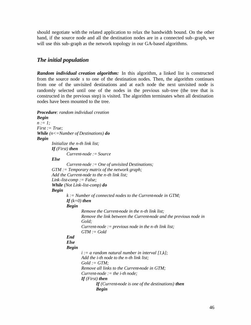
46

should negotiate with the related application to relax the bandwidth bound. On the other hand, if the source node and all the destination nodes are in a connected sub-graph, we will use this sub-graph as the network topology in our GA-based algorithms.

The initial population Random individual creation algorithm: In this algorithm, a linked list is constructed from the source node s to one of the destination nodes. Then, the algorithm continues from one of the unvisited destinations and at each node the next unvisited node is randomly selected until one of the nodes in the previous sub-tree (the tree that is constructed in the previous step) is visited. The algorithm terminates when all destination nodes have been mounted to the tree. Procedure: random individual creation Begin n := 1; First := True; While (n<=Number of Destinations) do Begin

Initialize the n-th link list; If (First) then

Current-node := Source Else

Current-node := One of unvisited Destinations; GTM := Temporary matrix of the network graph; Add the Current-node to the n-th link list; Link-list-comp := False; While (Not Link-list-comp) do Begin

k := Number of connected nodes to the Current-node in GTM; If (k=0) then Begin

Remove the Current-node in the n-th link list; Remove the link between the Current-node and the previous node in Gold; Current-node := previous node in the n-th link list; GTM := Gold

End Else Begin

i := a random natural number in interval [1,k]; Add the i-th node to the n-th link list; Gold := GTM; Remove all links to the Current-node in GTM; Current-node := the i-th node; If (First) then

If (Current-node is one of the destinations) then Begin

47

Link-list-comp := True; Make an individual by n-th link list; n := n+1; First := False; Mark the found destination as a visited destination

End Else

If (the Current-node is a node in one of the previous link lists(for example j -th link list)) then

{ if the Current-node has a connection to the source node, this link has higher priority}

Begin n-th link list := j -th link list from the source node to found position + Inverse (n_th link list); Link-list-comp := True;

Add the n-th link list to the individual; n := n+1; Mark this destination as a visited destination

End End {Else}

End {inner while} End {outer while} End {procedure}

The fitness function We define the fitness function for each individual, the tree T(s, M), using the penalty technique, as follows:

where a is a positive real coefficient, f(z) is the penalty function and ? is the degree of penalty (? is considered equal to 0.5).

Selection The selection process used here is based on spinning the roulette wheel pop-size times, and each time a single chromosome is selected as a new offspring. The probability Pi that a parent Ti is selected is given by:

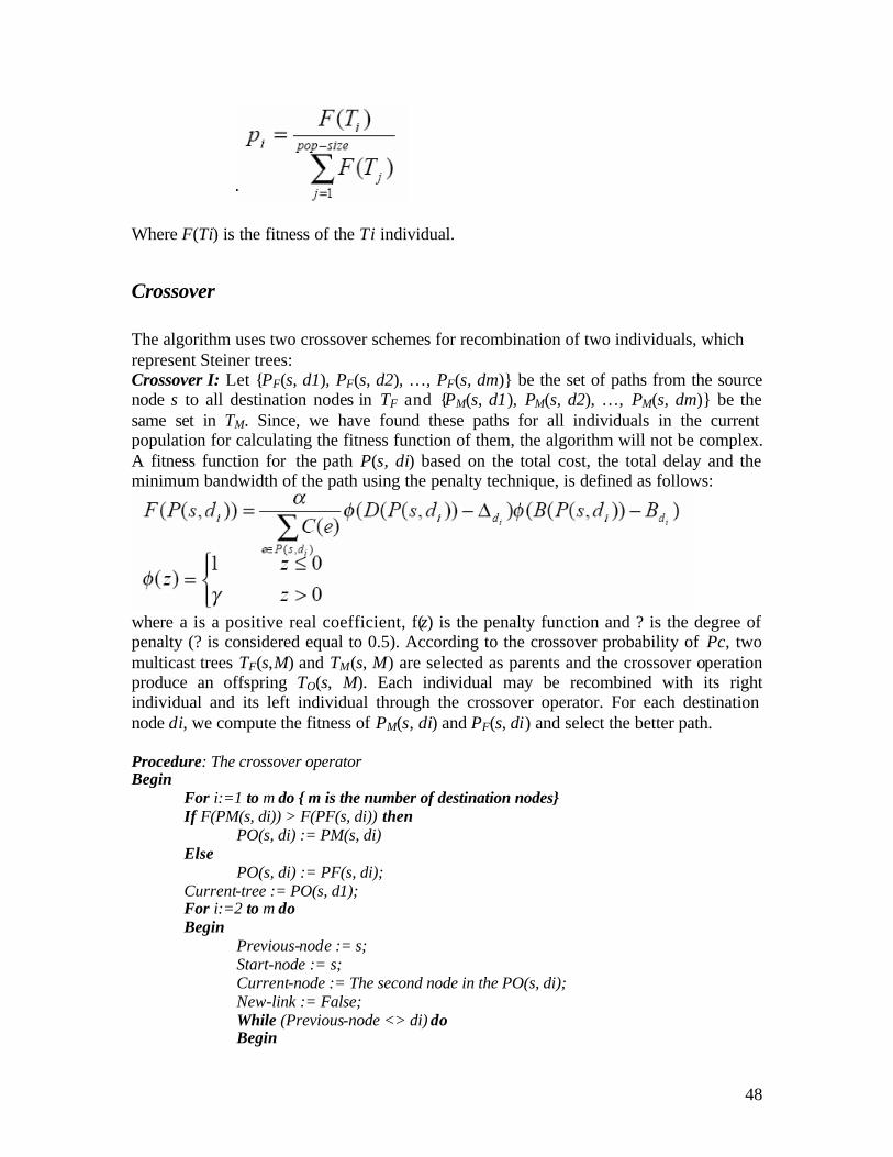
48

Where F(Ti) is the fitness of the Ti individual.

Crossover The algorithm uses two crossover schemes for recombination of two individuals, which represent Steiner trees: Crossover I: Let {PF(s, d1), PF(s, d2), …, PF(s, dm)} be the set of paths from the source node s to all destination nodes in TF and {PM(s, d1), PM(s, d2), …, PM(s, dm)} be the same set in TM. Since, we have found these paths for all individuals in the current population for calculating the fitness function of them, the algorithm will not be complex. A fitness function for the path P(s, di) based on the total cost, the total delay and the minimum bandwidth of the path using the penalty technique, is defined as follows:

where a is a positive real coefficient, f(z) is the penalty function and ? is the degree of penalty (? is considered equal to 0.5). According to the crossover probability of Pc, two multicast trees TF(s,M) and TM(s, M) are selected as parents and the crossover operation produce an offspring TO(s, M). Each individual may be recombined with its right individual and its left individual through the crossover operator. For each destination node di, we compute the fitness of PM(s, di) and PF(s, di) and select the better path. Procedure: The crossover operator Begin

For i:=1 to m do { m is the number of destination nodes} If F(PM(s, di)) > F(PF(s, di)) then

PO(s, di) := PM(s, di) Else

PO(s, di) := PF(s, di); Current-tree := PO(s, d1); For i:=2 to m do Begin

Previous-node := s; Start-node := s; Current-node := The second node in the PO(s, di); New-link := False; While (Previous-node <> di) do Begin

49

If the Current-node does not exist in the current-tree then Begin

Add the link between the Current-node and the Previous node to the current-tree; New-link := True;

End Else Begin

If the New-link = True then Remove all link from Start-node to the Previous-node in PO(s, di) in the current-tree; Start-node := Current-node New-link := False;

End Previous-node := Current-node; If there is another node in PO(s, di) then

Current-node := the next node in the PO(s, di) End

End End Crossover II: In this scheme, it is used a simple one-point crossover. The constructed offspring do not necessarily represent Steiner trees. Then, the effective and fast check and recovery algorithm proposed in Q. Zhang, Y.W. Lenug, "An orthogonal genetic algorithm for multimedia multicast routing" is used to connect the separate sub-trees in the offspring and also connecting the absent nodes of multicast group to the final tree.

Mutation There are two following algorithms for mutation operator: Mutation I: The mutation procedure randomly selects a subset of nodes and breaks the multicast tree into some separate sub-trees by removing all the links that are incident to the selected nodes. Then, the effective and fast check and recovery algorithm is used to connect the separate sub-trees and also connecting the absent nodes of multicast group to the final tree. Mutation II: According to the mutation probability Pm, the mutation procedure randomly selects an infeasible chromosome from one of the following class (If the first class is empty, a chromosome is selected from the second class and so on) • Class 1: The chromosomes, which do not satisfy the delay and the bandwidth constraints. • Class 2: The chromosomes, which do not satisfy the delay constraint. • Class 3: The chromosomes, which do not satisfy the bandwidth constraint. If all chromosomes in the current population satisfy both of the QoS constraints, we exit from the mutation procedure. Then, we select only the paths that satisfy both of the QoS constraints in the selected chromosome.

50

Implementation

In the current version of MonALISA the service that provide the data for the clients that are registered with them is done by means of a Proxy service. The proxy being also a service registers itself and it can be found by clients. The client finds such a Proxy and sends to it the request messages. Being connected to all the farms the proxy forwards to them and the result messages are sent back to the clients by using the Proxy service. The communication between the clients and the proxy and from the Proxy to the farms is done using TCP connections that are reliable. The use of proxy brings the following advantages:

• the use of Proxy reduces the number of TCP connections over the Internet. A farm has connections with each Proxy and not with all the clients. In this way a farm doesn’t uses a large number of threads as it would be the case when for each client a new connection would have been established

• by using a proxy even the farms that are behind a firewall can work; the farm connects to the Proxy and the messages sent by clients to the Proxy arrive to the farm

Being connected to all the proxies simultaneously, communication problems with a certain proxy allow the other proxies to use the farm. The distributed algorithms presented in this paper are running on farms as agents. They are started when a farm is launched in execution. As a distributed algorithm the nodes on which it runs need to communicate with each other in order to exchange the necessary information to build the minimum spanning tree or the multicast tree. In the current framework the communication between farms was not possible. As presented before in the current VRVS system the minimum spanning tree was computed in a centralized version that implied for a node (farm) to be aware of all the structure of the network in order to compute the tree. Therefore there was no need for communication between the nodes in establishing the minimum spanning tree. The first target of the implementation was to enable the farms to communicate between them when running the algorithm. Working in such a complex application such a change of the general architecture implied a lot of work in understanding precisely the use of each class and the relations between them. The main modifications were done in all the classes of the Proxy service and in the Data Cache Service of the farm. In the diagrams below is presented a schema about how the clients and the farms interact through the ProxyService represented here as a cloud, the UML of the Data Cache of the farm and the architecture of the Proxy Service.

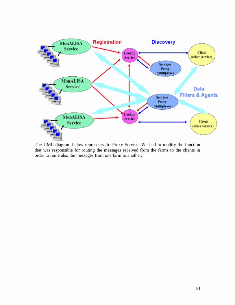
51

The UML diagram below represents the Proxy Service. We had to modify the function that was responsible for routing the messages received from the farms to the clients in order to route also the messages from one farm to another.

52

In the UML diagram below the Data Cache Service architecture is presented. The Cache uses a ProxyWorker :

• to verify the connections with the existing Proxy Services

• to establish connections with newly registered Proxy Services using a tcpClientWorker

• to send to each proxy a configuration update of a farm

• to send to each proxy a new result from the farm The ProxyWorker is important for our algorithm because it gives us the list of available proxies. These proxies are used for communication with the other nodes. When requested the ProxyWorker returns a connection to a ProxyService in order for the agent that runs the algorithm to send a message to another agent that runs on another farm (node) using the ProxyService as a router for the messages. One of the available Proxies is returned by the getProxyTCPClientWorker() method. The messages must arrive from one agent to another and we are not concerned by the ProxyService that is used for routing purposes.

53

The tcpClientWorker class has been modified in order to filter the messages from other farms. The agent that runs the algorithm register with the DataCache with 3 listener classes: one class used for synchronizing in the initial step the nodes that are involved in

54

the algorithm (SyncFarmMessagesListener), one class used for the messages that are received by a node from other nodes that belong to other fragments (OutFragmentFarmMessagesListener) and one class for the messages that are exchanged within the same fragment (InFragmentFarmMessagesListener). Each of this listeners implement the same interface FarmMessagesListener. The DataCache notifies each listener when a message of the specific type for each listener is received. Each listener implements in the notify method specific action for each type of message according to the algorithms described in the previous chapters. For these agents that run on each farm a new package was developed. For each algorithm an agent class has been implemented. Each agent class implements the same interface FarmAgentInterface in order to have a common base for other algorithm that will be developed in the future. In the UML diagram below the structure of this distributed MST is presented. For the messages that are used in these algorithms a new class was developed monMessageMST implementing the new interface for messages between farm agents monAgentMessage.

55

57

The data that is used in this algorithm is the one that is given by the ABPing module. In the configuration file of this module the list of adjacent farms for one farm is specified as a list like in the example below: wn1.rogrid.pub.ro 141.85.99.170 vrvs.co.pub.ro 141.85.99.136 141.85.99.170 wn1.rogrid.pub.ro vrvs.co.pub.ro vrvs.co.pub.ro 141.85.99.170 wn1.rogrid.pub.ro 141.85.99.136 wn1.rogrid.pub.ro For the algorithm the RTime value is extracted from the database. The formula behind this parameter is presented below:

This formula is flexible enough to permit calculating any kind of quality, based on RTT, Packet Loss and Jitter. The values obtained by pinging peers are:

• rtt – the round trip time for packets to travel to the peer and back;

• loss – percent, ranging from 0 to 1 of lost packets sent to the peer;

• jitter – sum of the variations of rtt for a set of samples, divided by the average rtt and number of samples

The list of available peers for each reflector and the *_COEF coefficients should be highly configurable to allow easy reconfiguration. To reach this goal, the configuration file is the same for all reflectors, each one knowing to extract only the information that is needed. The coefficients must be the same for all reflectors in order to obtain comparable RTime qualities. The configuration list is loaded at start from a URL configured in the Monalisa service and then it is checked periodically for changes.

58

Conclusions The algorithms implemented are going to be used in the VRVS system by specifying in the configuration file the one that is to be used. This approach offers a bigger flexibility and offers the possibility for further extensions. The algorithms can be extended to the case of oscillating links, etc. The presented genetic algorithm will also be implemented in a distributed version. Working for this diploma project has offered me the opportunity to do a research looking for a better solution than the one that existed in the beginning and also to face the difficulties of adapting the theoretical model to the existing framework and especially the difficulties of debugging the algorithm in a real distributed environment. I consider that this has been one of the most interesting experiences I have ever had combining in a unique way the skills of a software developer with the work of a researcher. Both the research and development parts are equally interesting each one having its strong points. I would also like to thank my coordinators Mr. Valentin CRISTEA and Mr. Iosif LEGRAND, to Mrs. Mihaela TOARTA, Mr. Catalin CARSTOIU and Mr. Ramiro VOICU for their constant help during this period.

59

References 1. Gallager, R. G. Humblet, Spira “A distributed algorithm for minimum spanning tree” ACM A transaction on programming language and systems,1983 2. E. Gafni “Improvements in the time complexity of two-message optimal election algorithms” Proceedings of 1985 PODC, 1985 3. F. Chin and H.F. Ting “An almost linear time and O( nlogn+e) messages distributed algorithm for minimum weight spanning tree”, 1985 4. B. Awerbuch “Optimal distributed algorithms for minimum weight spanning tree, counting, leader election and related problems” Proc. 19th Symp. on Theory of Computing, 1987 5. Gurdip Singh, Arthur J. Bernstein: A Highly Asynchronous Minimum Spanning Tree Protocol. Distributed Computing 8(3), 1994. 6. M. Faloutsos and M. Molle “Creating optimal distributed algorithms for minimum spanning trees”, 1995 7. Ramnik Bajaj, C. P. Ravikumar, Suresh Chandra Distributed Delay Constrained Multicast Path Setup Algorithm For High Speed Networks 8. A. T. Haghighat, K. Faez, M. Dehghan, A. Mowlaei, Y. Ghahremani A Genetic Algorithm for Steiner Tree Optimization with Multiple Constraints Using Prüfer Number 9. V. Kompella, J. Pasquale, and G. Polyzos. "Multicast Routing for multimedia communications", IEEE/ACM transactions on Networking, vol.1, no. 3, pp 286-292, Jun 1993. 10. F. Bauer and A. Varma. "Distributed Algorithms for Multicast Path Setup in Data Networks", IEEE-ACM transactions on Networking, 4(2), April 1996. 11. S. Voss. "Steiner's problem in graphs : Heuristic Methods", Discrete Applied Mathematics, vol.40, pp 45-72, 1992. 12. H. Takahashi and A. Matsuzama, "An approximate solution for the Steiner problem in graphs", Math.Japonica, vol 24, no.6, pp 573-577, 1980. 13. J. Kruskal, "On the shortest spanning subtree of a graph and the travelling salesman problem", Proc.Amer.Math.Soc, vol 7, pp 48-50, 1956. 14. B.K. Kadaba and J.M. Jaffe, "Routing to multiple destinations in computer networks", IEEE Trans.Comm., vol. COM-31(3), pp 343-351, March 1983 15. V. Kompella, J. Pasquale, and G. Polyzos. “Two Disrtibuted Algorithms for the constrained steiner tree problem”, Proc. Comp. Commun. Networking, San Diego, CA, Jun 1993. 16. M. Parsa, Q. Zhu, J.J. Garcia-Luna-Aceves, "An iterative algorithm for delay-constrained minimum-cost multicasting," IEEE/ACM Transactions on Networking, Vol. 6, No. 4, pp. 461-474, 1998. 17. Q. Sun, H. Langendörfer, "An efficient delay-constrained multicast routing algorithm," Journal of High-Speed Networks, Vol. 7, No. 1, pp. 43-55, 1998. 18. Q. Sun, "A genetic algorithm for delay-constrained minimum-cost multicasting," Technical Report, IBR, TU Braunschweig, Butenweg, 74/75, 38106, Braunschweig, Germany, 1999.

60

19. Z. Wang, B. Shi, E. Zhao, "Bandwidth-delay-constrainted least-cost multicast routing based on heuristic genetic algorithm," Computer Communications, Vol. 24, pp. 685-692, 2001 20. Catalin Carstoiu, “Monitoring and controlling the VRVS reflectors”, UPB, 2003 21. H.B. Newman, I.C.Legrand, P. Galvez, C.Carstoiu, R. Voicu, “MonALISA: A Distributed Monitoring Service Architecture”, Catech University & UPB, 2003 22. www.jini.org

61

Appendix

FarmAgentMST.java package lia.Monitor.FarmAgents; import java.util.Hashtable; import java.util.Vector; import net.jini.core.lookup.ServiceID; import net.jini.discovery.LookupDiscoveryManager; import java.util.logging.Logger; import java.util.logging.Level; import java.util.Comparator; import java.util.Collections; import lia.Monitor.DataCache.ProxyWorker; import lia.Monitor.monitor.FarmMessagesListener; import lia.Monitor.JiniSerFarmMon.RegFarmMonitor; import lia.Monitor.JiniSerFarmMon.MLLUSHelper; import lia.Monitor.monitor.monPredicate; import lia.Monitor.DataCache.Cache; import lia.Monitor.monitor.ExtendedResult; import lia.Monitor.monitor.monMessage; import lia.Monitor.monitor.monMessageMST; //class that computes a distributed minimum spanning tree //at the end of the algorithm each node running this algorithm knows the adjacent edges that are in the MST public class FarmAgentMST { /** Logger Name */ private static final transient String COMPONENT = "lia.Monitor.FarmAgents"; /** The Logger */ private static final transient Logger logger = Logger.getLogger(COMPONENT); private LookupDiscoveryManager ldm ; //used to translate a farm name to its ServiceID private MLLUSHelper resolver; //algorithm states private final int NOT_STARTED=-1; //the current node is searching for its best outgoing edge private final int FINDING=0; //the current node has sent the report message with its best outgoing edge private final int FOUND=1; //the current node has received the INITIATE1 message in the 2nd phase of the algorithm private final int INITIATE=2; //the current node has sent the FINISH message with the number of nodes in his subtree in the 2nd phase of the algorithm private final int FINISH=3; //the algorithm has finished private final int END=9; //the state of the algorithm private int state; //the phases of the algorithm private final int PHASE1=1; private final int PHASE2=2; //the phase of the algorithm private int phase;

62

//the class that launches this agent private RegFarmMonitor host ; //the dataStore of the current farm private Cache dataStore; //the ServiceID of the farm private ServiceID hostServiceID ; //hash the associates to each farm's ServiceID a FarmInfo object private Hashtable farms; //vector containing the unused farms sorted according to the value returned by ABPing for that farm private Vector unusedFarmList; //the root of the fragment the current node belongs to private ServiceID fragmentRoot; //the fragment's level private int fragmentLevel; //the level of the fragment the current node wants to connect to (2nd phase of the algorithm) private int otherFragmentLevel; //the syncListener is used to synchronize the current farm with the others according to the ABPingConfig file private SyncFarmMessagesListener syncListener; //these listeners are used for the messages within or from outside the fragment private OutFragmentFarmMessagesListener outListener; private InFragmentFarmMessagesListener inListener; //the farms that belong to the current's node part of the MST private Vector MSTFarmList; //a ProxyWorker keeps all the connections to all the proxies //it is used to send a message private ProxyWorker proxyWorker; //keeps the number of nodes to/from which a message has been sent/received private int findCount; //keeps the actual number of nodes in the subtree rooted at the current node private int findCountTotal; //the ServiceID of the parent node private ServiceID inBranch; //the ServiceID of the best farm discovered by the current node private ServiceID bestFarm; //the ABPing value for the bestFarm private double bestFarmValue; //the path to the bestFarm from the current node (used in the changeRoot procedure) private Vector bestFarmPath; //the ServiceID of the current best farm of the node private ServiceID testFarm; //the ABPing value for the testFarm private double testFarmValue; //the vector with the farms the current node has already synced with protected Vector sync; //class containg the farm's name and the ABPing value private class FarmInfo{ private String farmName; private double avgABPingValue; public FarmInfo(String name,double value){ this.farmName=name; this.avgABPingValue=value; } public String getFarmName(){ return farmName; }

63

public double getAvgABPingValue(){ return avgABPingValue; } public void setAvgABPingValue(double value){ avgABPingValue=value; } public String toString(){ String temp=new String("["+farmName+" = "+avgABPingValue+"]"); return temp; } } //class used for synchronizing with the other farms private class SyncFarmMessagesListener implements FarmMessagesListener{ public synchronized void notify(monMessage msg){ monMessageMST MSTmsg=(monMessageMST)msg.ident; if(msg.tag.equals("SYNC")){ //if the algorithm has not started for the current node the message is delayed if(state==NOT_STARTED){ dataStore.addSyncFarmMessage(msg); //logger.log(Level.INFO,"Synced delayed "+MSTmsg.getSourceServiceID()); } else //if the farm is not synchronized with the farm from which it has received the sync message //then it sends a sync message, it adds the farm to the current list of farms the node has already synced with //and it mediates his ABPing value for that node with the value received from the other node if(!isSynced(MSTmsg.getSourceServiceID())){ sendSync(MSTmsg.getSourceServiceID(),getFarmABPingValue(MSTmsg.getSourceServiceID())); sync.add(MSTmsg.getSourceServiceID()); avgABPingValue(MSTmsg.getSourceServiceID(),MSTmsg.getABPingValue()); // logger.log(Level.INFO,"Synced with "+MSTmsg.getSourceServiceID()); } } } } //class used to handle the messages received from another fragment private class OutFragmentFarmMessagesListener implements FarmMessagesListener{ public synchronized void notify(monMessage msg){ //the MST message monMessageMST MSTmsg=(monMessageMST)msg.ident; logger.log(Level.INFO,"< "+msg.tag+" from "+getFarmName(MSTmsg.getSourceServiceID())+" myLevel="+fragmentLevel+" myFragmentRoot="+getFarmName(fragmentRoot)); //CONNECT message if(msg.tag.equals("CONNECT")){ logger.log(Level.INFO,"CONNECT from level="+MSTmsg.getLevel()+" fragmentRoot="+getFarmName(MSTmsg.getFragmentRoot()));

64

if(phase==PHASE1){ //if the other fragment's level is smaller than our fragment level if(MSTmsg.getLevel()<fragmentLevel){ //we have a submission from the other fragment logger.log(Level.INFO,"SUBMISSION from "+getFarmName((ServiceID)MSTmsg.getSourceServiceID())); //if the farm is still in the unusedFarmList we remove it since it will already be in our MST if(getFarmIndex(MSTmsg.getSourceServiceID())!=-1){ MSTFarmList.add(getFarmServiceID((ExtendedResult)unusedFarmList.remove(getFarmIndex(MSTmsg.getSourceServiceID())))); logger.log(Level.INFO,"Added in MST "+getFarmName((ServiceID)MSTFarmList.elementAt(MSTFarmList.size()-1))); } else //if the farm that has done the submission was our testFarm we add the farm in our MST if(compareServiceIDs(testFarm,MSTmsg.getSourceServiceID())==0){ MSTFarmList.add(MSTmsg.getSourceServiceID()); logger.log(Level.INFO,"Added in MST "+getFarmName((ServiceID)MSTFarmList.elementAt(MSTFarmList.size()-1))); } //we are sending the INITIATE message along with our fragmentLevel and fragmentRoot monMessageMST initiateMSTmsg=new monMessageMST(hostServiceID,MSTmsg.getSourceServiceID(),new Integer(fragmentLevel),fragmentRoot,new Integer(state)); sendMessage(initiateMSTmsg,"INITIATE"); //if we are in the FINDING state we also add the new fragment in this procedure if(state==FINDING) findCount++; } //if the other fragment's level >= our current level else{ //if the edge is not in the unusedFarmList then it is also our best outgoing edge if(getFarmIndex(MSTmsg.getSourceServiceID())==-1){ //we have an EQUIJOIN //if we have a smaller ID then we become the new root of the fragment and we initiate another step if(compareServiceIDs(fragmentRoot,MSTmsg.getFragmentRoot())<0){ fragmentLevel++; state=FINDING; logger.log(Level.INFO,"EQUI JOIN =>Incrementing level to "+fragmentLevel); initiate(); } } //the other's fragment level > our current level then the CONNECT message is delayed

65

else{ logger.log(Level.INFO,"CONNECT delayed"); dataStore.addOutFragmentFarmMessage(msg); } } }//end if PHASE1 else{ //if the other fragment's level > our fragment level the CONNECT is delayed if(MSTmsg.getLevel()>fragmentLevel){ logger.log(Level.INFO,"CONNECT delayed"); dataStore.addFarmMessage(msg); } else{ //if the node is in INITIATE state then the other fragment is included in the current INITIATE1 step if(state==INITIATE){ monMessageMST initiateMsg= new monMessageMST(hostServiceID,MSTmsg.getSourceServiceID(),new Integer(fragmentLevel),fragmentRoot); sendMessage(initiateMsg,"INITIATE1"); findCount++; } else //if the node has sent the FINISH message and the other fragment's level < our level - log(our level) if((state==FINISH ||state==FINDING||state==FOUND) && MSTmsg.getLevel()<fragmentLevel-Math.log(fragmentLevel)){ monMessageMST initiateMsg=new monMessageMST(hostServiceID,MSTmsg.getSourceServiceID(),new Integer(fragmentLevel),fragmentRoot); //we instruct the other node to do a counting of the nodes and to decide after that if it still wants to join sendMessage(initiateMsg,"COUNT"); //if the REPORT message has not been sent yet we wait for a decision if(state==FINDING) findCount++; } else //if the node has sent the FINISH message and the other fragment's level >= our level - log(our level) then the other fragment //cannot participate in the current iteration of our fragment //the joining fragment is added in the MST and it is instructed to start the first phase if((state==FINISH ||state==FINDING||state==FOUND) && fragmentLevel>=MSTmsg.getLevel() && MSTmsg.getLevel()>=(fragmentLevel-Math.log(fragmentLevel))){ if(getFarmIndex(MSTmsg.getSourceServiceID())!=-1){ MSTFarmList.add(getFarmServiceID((ExtendedResult)unusedFarmList.remove(getFarmIndex(MSTmsg.getSourceServiceID())))); logger.log(Level.INFO,"Added in MST "+getFarmName((ServiceID)MSTFarmList.elementAt(MSTFarmList.size()-1))); } else if(compareServiceIDs(testFarm,MSTmsg.getSourceServiceID())==0){ MSTFarmList.add(MSTmsg.getSourceServiceID()); logger.log(Level.INFO,"Added in MST

66

"+getFarmName((ServiceID)MSTFarmList.elementAt(MSTFarmList.size()-1))); } monMessageMST initiateMsg=new monMessageMST(hostServiceID,MSTmsg.getSourceServiceID(),new Integer(fragmentLevel),fragmentRoot); sendMessage(initiateMsg,"INITIATE1"); } } }//end else PHASE2 } else if(msg.tag.equals("TEST")){ logger.log(Level.INFO,"TEST from level="+MSTmsg.getLevel()+" fragmentRoot="+getFarmName(MSTmsg.getFragmentRoot())); //if we are in the first phase of the algorithm we delay a TEST message until our level becomes >= then the other fragment's level //if we are in the second phase of the algorithm we delay a TEST message until our level becomes at least the OF level - log(OF level) OF=other fragment if(((phase==PHASE2&&(MSTmsg.getLevel()-Math.log(MSTmsg.getLevel())>fragmentLevel)) ||(phase==PHASE1&&MSTmsg.getLevel()>fragmentLevel)) &&compareServiceIDs(MSTmsg.getFragmentRoot(),fragmentRoot)!=0){ logger.log(Level.INFO,"TEST delayed "); dataStore.addOutFragmentFarmMessage(msg); } else //if the to fragments have the same fragment root a REJECT message is sent //and the correspondig entry in the unusedFarmList is removed if it exists //if this edge was our test edge we test another edge if(compareServiceIDs(MSTmsg.getFragmentRoot(),fragmentRoot)==0){ monMessageMST rejectMSTmsg=new monMessageMST(hostServiceID,MSTmsg.getSourceServiceID()); sendMessage(rejectMSTmsg,"REJECT"); for(int i=0;i<unusedFarmList.size();i++){ ExtendedResult crtRes=(ExtendedResult)unusedFarmList.elementAt(i); if(compareServiceIDs(resolver.getServiceIDfromFarm(crtRes.NodeName),MSTmsg.getSourceServiceID())==0){ //logger.log(Level.INFO,"Scot "+resolver.getServiceIDfromFarm(crtRes.NodeName)); logger.log(Level.INFO,"Removing "+crtRes.NodeName); unusedFarmList.remove(i); break; } } if(testFarm!=null) if(compareServiceIDs(testFarm,MSTmsg.getSourceServiceID())==0) test(); } //if all the conditions are meet a ACCEPT message is sent else{

67

monMessageMST acceptMSTmsg=new monMessageMST(hostServiceID,MSTmsg.getSourceServiceID()); sendMessage(acceptMSTmsg,"ACCEPT"); } } else if(msg.tag.equals("ACCEPT")){ //if we receive a positive answer we update the best farm or try to send a report if(bestFarmValue>testFarmValue){ bestFarmValue=testFarmValue; bestFarm=testFarm; testFarm=null; } report(); } else if(msg.tag.equals("REJECT")){ //if we receive a reject message that has not expired we start the testing procedure if(compareServiceIDs(testFarm,MSTmsg.getSourceServiceID())==0) test(); } else if(msg.tag.equals("REJECTCONNECT")){ //if the connect message was received in a FINDING step then the current node can continue if(state==FINDING) findCount--; } else if(msg.tag.equals("ACCEPTCONNECT")){ //we add the edge in the MST and if we are in a FINDING state we also put to work the joining fragment if(getFarmIndex(MSTmsg.getSourceServiceID())!=-1){ MSTFarmList.add(getFarmServiceID((ExtendedResult)unusedFarmList.remove(getFarmIndex(MSTmsg.getSourceServiceID())))); logger.log(Level.INFO,"Added in MST "+getFarmName((ServiceID)MSTFarmList.elementAt(MSTFarmList.size()-1))); } else if(compareServiceIDs(testFarm,MSTmsg.getSourceServiceID())==0){ MSTFarmList.add(MSTmsg.getSourceServiceID()); logger.log(Level.INFO,"Added in MST "+getFarmName((ServiceID)MSTFarmList.elementAt(MSTFarmList.size()-1))); } if(state==FINDING){ findCount++; monMessageMST initiateMsg=new monMessageMST(hostServiceID,MSTmsg.getSourceServiceID(),new Integer(fragmentLevel)); sendMessage(initiateMsg,"INITIATE2"); } } } }

68

//class that handles messages within the fragment private class InFragmentFarmMessagesListener implements FarmMessagesListener{ public void notify(monMessage msg){ monMessageMST MSTmsg=(monMessageMST)msg.ident; logger.log(Level.INFO,"< "+msg.tag+" from "+getFarmName(MSTmsg.getSourceServiceID())+" myLevel="+fragmentLevel+" myFragmentRoot="+getFarmName(fragmentRoot)); if(msg.tag.equals("INITIATE")){ //upon receiving an INITIATE message the node's fragmentLevel,fragmentRoot,inBranch and state are updated //and this message is also sent to all its children fragmentLevel=MSTmsg.getLevel(); fragmentRoot=MSTmsg.getFragmentRoot(); inBranch=MSTmsg.getSourceServiceID(); state=MSTmsg.getState(); //logger.log(Level.INFO,"state="+state); initiate(); } else if(msg.tag.equals("INITIATE1")){ //similar to the initiate message but for the 2nd phase of the algorithm phase=PHASE2; fragmentLevel=MSTmsg.getLevel(); fragmentRoot=MSTmsg.getFragmentRoot(); inBranch=MSTmsg.getSourceServiceID(); initiate1(); } else if(msg.tag.equals("FINISH")){ //the number of nodes from which a finish message is expected is decremented //and the total number of farms in the subtree is updated findCount--; findCountTotal+=MSTmsg.getFarms(); //if the node is not the root of the fragment it sends the gathered information to its parent if(compareServiceIDs(fragmentRoot,hostServiceID)!=0) finish(); else{ //the root updates the fragment's level fragmentLevel=(int)Math.log(findCountTotal+1); //if in the 2nd phase of the algorithm the INITIATE message is sent if(state==INITIATE) initiate2(); else if(state==FOUND){ //if in the 1st phase of the algorithm and the fragment's level is bigger than the level of the fragment it wants to //join with it sends a REJECTCONNECT message and starts a new iteration if(fragmentLevel>=otherFragmentLevel){ monMessageMST rejectMsg=new monMessageMST(hostServiceID,bestFarm); sendMessage(rejectMsg,"REJECTCONNECT"); initiate1(); } else if(fragmentLevel<otherFragmentLevel){ //it sends a ACCEPTCONNECT message and updates its level, root and MST list and starts the update procedure

69

monMessageMST connectMsg=new monMessageMST(hostServiceID,bestFarm,new Integer(fragmentLevel)); sendMessage(connectMsg,"ACCEPTCONNECT"); fragmentRoot=bestFarm; fragmentLevel=otherFragmentLevel; MSTFarmList.add(bestFarm); update(); } } } } else if(msg.tag.equals("UPDATE")){ //upon receiving a UPDATE message the information is updating and sent to all the subtree fragmentLevel=MSTmsg.getLevel(); fragmentRoot=MSTmsg.getFragmentRoot(); inBranch=MSTmsg.getSourceServiceID(); update(); } else if(msg.tag.equals("INITIATE2")){ //the node updates its level and starts the procedure initiate2 fragmentLevel=MSTmsg.getLevel(); initiate2(); } else if(msg.tag.equals("REPORT")){ //upon receiving a REPORTmessage the node checks if it is from its subtree boolean fromSons=false; if(inBranch==null) fromSons=true; else if(compareServiceIDs(MSTmsg.getSourceServiceID(),inBranch)!=0) fromSons=true; if(fromSons){ //decrements the number of nodes from which it waits for a report //and updates the number of nodes in its subtree findCount--; findCountTotal+=MSTmsg.getFarms(); //if the report actually contains an edge the bestFarm is updated if(MSTmsg.getBestFarmPath()!=null) if(MSTmsg.getBestFarmValue()<bestFarmValue){ bestFarmValue=MSTmsg.getBestFarmValue(); bestFarm=MSTmsg.getDestinationServiceID(); bestFarmPath=MSTmsg.getBestFarmPath(); } //if the current node is not the root of the fragment the report is sent to its parent if(compareServiceIDs(fragmentRoot,hostServiceID)!=0) report(); else if(findCount==0){ //if the root has received all the reports and the bestFarm==Double.MAX_VALUE //then the algorithm is finished //the root displays its MST edges and sents this info to all its children if(Math.abs(Double.MAX_VALUE-bestFarmValue)<1.0){

70

state=END; logger.log(Level.INFO,"ALGORITHM FINISHED!!!"); for(int i=0;i<MSTFarmList.size();i++){ logger.log(Level.INFO,"edge="+getFarmName((ServiceID)MSTFarmList.elementAt(i))); monMessageMST endMsg=new monMessageMST(hostServiceID,(ServiceID)MSTFarmList.elementAt(i)); sendMessage(endMsg,"END"); } } else{ //if a best edge has been found but the reports show that a bigger number of nodes than the one estimated by the level //the initiate step is repeated state=FOUND; if(findCountTotal>=Math.pow(2,fragmentLevel)){ while(findCountTotal>=Math.pow(2,fragmentLevel)) fragmentLevel++; state=FINDING; initiate(); } else changeRoot(); } } } else if(state==FINDING) dataStore.addFarmMessage(msg); } else if(msg.tag.equals("CHANGEROOT")){ //as the changeroot message trickles down the tree to the specified edge the parent -son relation is changed //and when it arrives to the specified node that one sends the CONNECT message if(MSTmsg.getBestFarmPath().size()==0){ if(phase==PHASE1){ MSTFarmList.add(bestFarm); logger.log(Level.INFO,"Added in MST "+getFarmName((ServiceID)MSTFarmList.elementAt(MSTFarmList.size()-1))); } monMessageMST connectMSTmsg=new monMessageMST(hostServiceID,bestFarm); sendMessage(MSTmsg," CONNECT"); } else changeRoot(); } else if(msg.tag.equals("END")){ //each node sends the message to all children and shows the edges in the MST logger.log(Level.INFO,"ALGORITHM FINISHED");

71

for(int i=0;i<MSTFarmList.size();i++){ logger.log(Level.INFO,"edge="+getFarmName((ServiceID)MSTFarmList.elementAt(i))); if(compareServiceIDs(MSTmsg.getSourceServiceID(),(ServiceID)MSTFarmList.elementAt(i))!=0){ monMessageMST endMsg=new monMessageMST(hostServiceID,(ServiceID)MSTFarmList.elementAt(i)); sendMessage(endMsg,"END"); } } } else if(msg.tag.equals("COUNT")){ //the root keeps the other fragment's level and each node sends to all children the count message if(compareServiceIDs(hostServiceID,fragmentRoot)==0) otherFragmentLevel=MSTmsg.getLevel(); count(); } } } //constructor of the class public FarmAgentMST(){ unusedFarmList=new Vector(); farms= new Hashtable(); MSTFarmList=new Vector(); sync=new Vector(); state=NOT_STARTED; phase=PHASE1; } //returns the serviceID of a farm from the ABPing result private ServiceID getFarmServiceID(ExtendedResult res){ return resolver.getServiceIDfromFarm(res.NodeName); } //compares 2 serviceID as strings and returns this value private int compareServiceIDs(ServiceID sid1,ServiceID sid2){ return sid1.toString().compareTo(sid2.toString()); } //initialization of the variables public void init(LookupDiscoveryManager ldm, RegFarmMonitor host, ServiceID hostServiceID){ this.ldm=ldm; this.host=host; this.hostServiceID=hostServiceID; this.dataStore=(Cache) host.dataStore; //the listeners are registered with the dataStore outListener=new OutFragmentFarmMessagesListener(); inListener=new InFragmentFarmMessagesListener(); syncListener= new SyncFarmMessagesListener(); dataStore.setInFragmentListener(inListener); dataStore.setOutFragmentListener(outListener); dataStore.setSyncListener(syncListener); } //verifies if a farm given by its serviceID is synced with our farm private boolean isSynced(ServiceID sid){ int i;

72

for(i=0;i<sync.size();i++) if(compareServiceIDs(sid,(ServiceID)sync.elementAt(i))==0) return true; return false; } //sends a SYNC message containing our ABPing value for the destination farm private void sendSync(ServiceID sid,double value){ monMessageMST syncMSTmsg=new monMessageMST(hostServiceID,sid,new Double(value)); sendMessage(syncMSTmsg,"SYNC"); } //retrieves the ABPing values from the database private void getData(){ String[] params=new String[1]; params[0]=new String("RTime"); Vector results=dataStore.select(new monPredicate("*","ABPing","*",-60000,-1,params,null)); // logger.log(Level.INFO,"ABPing no. of results="+results.size()); for(int i=results.size()-1;i>=0;i--){ ExtendedResult res=(ExtendedResult)results.elementAt(i); ServiceID farmSID=resolver.getServiceIDfromFarm(res.NodeName); if(farmSID!=null) if(!farms.containsKey(farmSID)){ farms.put(farmSID,new FarmInfo(res.NodeName,res.param[0])); unusedFarmList.add(res); } } logger.log(Level.INFO,"farms="+farms); } //updates the ABPing value with the value received in the SYNC message private void avgABPingValue(ServiceID sid,double value){ ExtendedResult res=(ExtendedResult)unusedFarmList.remove(getFarmIndex(sid)); FarmInfo farmInfo=(FarmInfo)farms.get(sid); res.param[0]=(res.param[0]+value)/2.0; farmInfo.setAvgABPingValue(res.param[0]); unusedFarmList.insertElementAt(res,0); } //sorts the edge acording to their ABPing values private void sortData(){ // logger.log(Level.INFO,"After filtering the data no. of results="+unusedFarmList.size()); for(int i=0;i<unusedFarmList.size();i++) // logger.log(Level.INFO,((ExtendedResult)unusedFarmList.elementAt(i)).NodeName+"="+((ExtendedResult)unusedFarmList.elementAt(i)).param[0]); Collections.sort(unusedFarmList,new Comparator(){ public int compare(Object o1,Object o2){ ExtendedResult res1=(ExtendedResult)o1; ExtendedResult res2=(ExtendedResult)o2; if(res1.param[0]==res2.param[0]) return res1.NodeName.compareTo(res2.NodeName); if(res1.param[0]>res2.param[0]) return 1; return -1; } }); logger.log(Level.INFO,"After sorting the data no. of results="+unusedFarmList.size()); for(int i=0;i<unusedFarmList.size();i++)

73

logger.log(Level.INFO,((ExtendedResult)unusedFarmList.elementAt(i)).NodeName+"="+((ExtendedResult)unusedFarmList.elementAt(i)).param[0]); } //the wakeup procedure private void wakeup(){ //initialization fragmentLevel=0; fragmentRoot=hostServiceID; findCount=0; //data fetching getData(); state=FOUND; //synchronization sync(); sortData(); testFarm=null; testFarmValue=Double.MAX_VALUE; MSTFarmList.add(getFarmServiceID((ExtendedResult)unusedFarmList.remove(0))); logger.log(Level.INFO,"Added in MST "+getFarmName((ServiceID)MSTFarmList.elementAt(MSTFarmList.size()-1))); monMessageMST MSTmsg=new monMessageMST(hostServiceID,(ServiceID)MSTFarmList.elementAt(0),new Integer(fragmentLevel),fragmentRoot); sendMessage(MSTmsg,"CONNECT"); } //SYNC messages are sent until the synchronization is done with all the other farms private void sync(){ while(sync.size()!=unusedFarmList.size()){ for (int i=0;i<unusedFarmList.size();i++){ ExtendedResult res=(ExtendedResult)unusedFarmList.elementAt(i); ServiceID crtFarmSID=getFarmServiceID(res); if(!isSynced(crtFarmSID)) sendSync(crtFarmSID,res.param[0]); try{ Thread.sleep(500); } catch(Exception e){ e.printStackTrace(); } } try{ Thread.sleep(1000); } catch(Exception e){ e.printStackTrace(); } } logger.log(Level.INFO,"SYNCED with the others"); } //the counting procedure sends the COUNT message to all the children private void count(){ findCount=0; findCountTotal=0; for(int i=0;i<MSTFarmList.size();i++){ if(inBranch!=null){ if(compareServiceIDs((ServiceID)MSTFarmList.elementAt(i),inBranch)!=0){ monMessageMST initiateMsg=new monMessageMST(hostServiceID,(ServiceID)MSTFarmList.elementAt(i),new Integer(fragmentLevel),fragmentRoot);

74

sendMessage(initiateMsg,"COUNT"); findCount++; } } else{ monMessageMST initiateMsg=new monMessageMST(hostServiceID,(ServiceID)MSTFarmList.elementAt(i),new Integer(fragmentLevel),fragmentRoot); sendMessage(initiateMsg,"COUNT"); findCount++; } } finish(); } //the update procedure sends an UPDATE message to all children but no reply is waited private void update(){ for(int i=0;i<MSTFarmList.size();i++){ if(inBranch!=null){ if(compareServiceIDs((ServiceID)MSTFarmList.elementAt(i),inBranch)!=0){ monMessageMST initiateMsg=new monMessageMST(hostServiceID,(ServiceID)MSTFarmList.elementAt(i),new Integer(fragmentLevel),fragmentRoot); sendMessage(initiateMsg,"UPDATE"); } } else{ monMessageMST initiateMsg=new monMessageMST(hostServiceID,(ServiceID)MSTFarmList.elementAt(i),new Integer(fragmentLevel),fragmentRoot); sendMessage(initiateMsg,"UPDATE"); } } } //the initiate1 procedure sends the level and the root of the fragment to all children and waits for a FINISH message //from all of them private void initiate1(){ state=INITIATE; bestFarm=null; bestFarmValue=Double.MAX_VALUE; bestFarmPath=null; findCount=0; findCountTotal=0; for(int i=0;i<MSTFarmList.size();i++){ if(inBranch!=null){ if(compareServiceIDs((ServiceID)MSTFarmList.elementAt(i),inBranch)!=0){ monMessageMST initiateMsg=new monMessageMST(hostServiceID,(ServiceID)MSTFarmList.elementAt(i),new Integer(fragmentLevel),fragmentRoot); sendMessage(initiateMsg,"INITIATE1"); findCount++; } } else{ monMessageMST initiateMsg=new monMessageMST(hostServiceID,(ServiceID)MSTFarmList.elementAt(i),new Integer(fragmentLevel),fragmentRoot); sendMessage(initiateMsg,"INITIATE1"); findCount++; } } finish(); }

75

//the initiate2 procedure sends the updated level to all the children and starts the testing procedure and waits //a REPORT message with the best outgoing edge from all of them private void initiate2(){ state=FINDING; findCount=0; findCountTotal=0; for(int i=0;i<MSTFarmList.size();i++){ if(inBranch!=null){ if(compareServiceIDs((ServiceID)MSTFarmList.elementAt(i),inBranch)!=0){ monMessageMST initiateMsg=new monMessageMST(hostServiceID,(ServiceID)MSTFarmList.elementAt(i),new Integer(fragmentLevel),fragmentRoot); sendMessage(initiateMsg,"INITIATE2"); findCount++; } } else{ monMessageMST initiateMsg=new monMessageMST(hostServiceID,(ServiceID)MSTFarmList.elementAt(i),new Integer(fragmentLevel),fragmentRoot); sendMessage(initiateMsg,"INITIATE2"); findCount++; } } test(); } //when the FINISH message has been received from all the children //a FINISH message is also sent to the parent private void finish(){ if (findCount==0){ monMessageMST finishMsg=new monMessageMST(hostServiceID,inBranch,new Integer(findCountTotal+1)); sendMessage(finishMsg,"FINISH"); state=FINISH; } } //the initiate message informs all the children of the level and the root of the fragment and upon receiving this //message each node starts finding the best outgoing edge //after receiving this value from all the children a report message is sent to the parent with the best outgoing edge //in the subtree rooted at the current node private void initiate(){ int MSTsize=MSTFarmList.size(); bestFarm=null; bestFarmValue=Double.MAX_VALUE; bestFarmPath=null; findCount=0; findCountTotal=0; for(int i=0;i<MSTsize;i++){ ServiceID crtFarmServiceID; crtFarmServiceID=(ServiceID)MSTFarmList.elementAt(i); if(inBranch!=null){ if(compareServiceIDs(crtFarmServiceID,inBranch)!=0){ monMessageMST initiateMSTmsg=new monMessageMST(hostServiceID,crtFarmServiceID,new Integer(fragmentLevel),fragmentRoot,new Integer(state)); sendMessage(initiateMSTmsg,"INITIATE"); if(state==FINDING) findCount++; }

76

} else{ monMessageMST initiateMSTmsg=new monMessageMST(hostServiceID,crtFarmServiceID,new Integer(fragmentLevel),fragmentRoot,new Integer(state)); sendMessage(initiateMSTmsg,"INITIATE"); if(state==FINDING) findCount++; } } if(state==FINDING) test(); } //the node takes an edge from the unusedFarmList and tests to see if it is valid private void test(){ if(unusedFarmList.size()>0){ ExtendedResult nextRes=(ExtendedResult)unusedFarmList.remove(0); testFarm=getFarmServiceID(nextRes); testFarmValue=nextRes.param[0]; monMessageMST testMSTmsg=new monMessageMST(hostServiceID,testFarm,new Integer(fragmentLevel),fragmentRoot); sendMessage(testMSTmsg,"TEST"); } else{ testFarm=null; //if all my edges were tested I check to see if all the reports were received report(); } } //the report procedure when the best outgoing edge of each node is sent back to the root private void report(){ //logger.log(Level.INFO,"find="+findCount+" test="+testFarm); //if the reports from all children have been received //the report is sent to the parent if(findCount==0 && testFarm==null){ state=FOUND; if(bestFarm!=null){ if( bestFarmPath==null) bestFarmPath=new Vector(); bestFarmPath.add(hostServiceID); } monMessageMST reportMSTmsg=new monMessageMST(hostServiceID,inBranch,new Double(bestFarmValue),bestFarm,bestFarmPath,new Integer(findCountTotal+1)); sendMessage(reportMSTmsg,"REPORT"); } } //the message is sent to the next node according to the path received in the message private void changeRoot(){ inBranch=(ServiceID)bestFarmPath.elementAt(bestFarmPath.size()-1); bestFarmPath.remove(bestFarmPath.size()-1); monMessageMST changeRootMSTmsg=new monMessageMST(hostServiceID,inBranch,bestFarmPath); sendMessage(changeRootMSTmsg,"CHANGEROOT"); } //the entry point in the algorithm that starts the node public void doWork(){

77

proxyWorker=dataStore.getProxyWorker(); resolver=MLLUSHelper.getInstance(); wakeup(); } //returns the farm's name given its ServiceID private String getFarmName(ServiceID sid){ if(farms.containsKey(sid)) return ((FarmInfo)farms.get(sid)).getFarmName(); return sid.toString(); } //returns the ABPingValue for a farm given its ServiceID private double getFarmABPingValue(ServiceID sid){ return ((FarmInfo)farms.get(sid)).getAvgABPingValue(); } //gets a farm index in the unusedFarmList using its ServiceID private int getFarmIndex(ServiceID sid){ for(int i=0;i<unusedFarmList.size();i++) if(compareServiceIDs(getFarmServiceID((ExtendedResult)unusedFarmList.elementAt(i)),sid)==0) return i; return -1; } //sends a message using a proxy given by the ProxyWorker private void sendMessage(monMessageMST MSTmsg,String tag){ if(tag.compareTo("SYNC")!=0) logger.log(Level.INFO,"> "+tag+" to "+getFarmName(MSTmsg.getDestinationServiceID())); monMessage msg=new monMessage(tag,MSTmsg,null); proxyWorker.getProxyTCPClientWorker().sendMessage(msg); //we force the treatment of the delayed messages dataStore.addFarmMessage(new monMessage("boogie",new monMessageMST(hostServiceID,hostServiceID),null)); } } FarmAgentInterface.java package lia.Monitor.FarmAgents; import lia.Monitor.JiniSerFarmMon.RegFarmMonitor; import net.jini.core.lookup.ServiceItem; import net.jini.discovery.LookupDiscoveryManager; public interface FarmAgentInterface { public void init(LookupDiscoveryManager ldm, RegFarmMonitor host, ServiceItem ser_host); public void doWork(); } monMessageMST.java package lia.Monitor.monitor;

78

import java.util.Vector; import net.jini.core.lookup.ServiceID; import lia.Monitor.monitor.monAgentMessage; public class monMessageMST extends monAgentMessage implements java.io.Serializable { public ServiceID fromFarmServiceID; public ServiceID toFarmServiceID; public Integer level; public Double bestFarmValue; public Double ABPingValue; public ServiceID bestFarm; public ServiceID fragmentRoot; public Integer farms; public Integer state; public Vector bestFarmPath; public monMessageMST(){ } public monMessageMST(ServiceID fromFarmServiceID,ServiceID toFarmServiceID,Integer level,ServiceID fragmentRoot,Integer state){ this.fromFarmServiceID=fromFarmServiceID; this.toFarmServiceID=toFarmServiceID; this.level=level; this.fragmentRoot=fragmentRoot; this.state=state; } public monMessageMST(ServiceID fromFarmServiceID,ServiceID toFarmServiceID,Integer level,ServiceID fragmentRoot){ this.fromFarmServiceID=fromFarmServiceID; this.toFarmServiceID=toFarmServiceID; this.level=level; this.fragmentRoot=fragmentRoot; } public monMessageMST(ServiceID fromFarmServiceID,ServiceID toFarmServiceID,Double ABPingValue){ this.fromFarmServiceID=fromFarmServiceID; this.toFarmServiceID=toFarmServiceID; this.ABPingValue=ABPingValue; } public monMessageMST(ServiceID fromFarmServiceID,ServiceID toFarmServiceID){ this.fromFarmServiceID=fromFarmServiceID; this.toFarmServiceID=toFarmServiceID; } public monMessageMST(ServiceID fromFarmServiceID,ServiceID toFarmServiceID,Vector bestFarmPath){ this.fromFarmServiceID=fromFarmServiceID; this.toFarmServiceID=toFarmServiceID; this.bestFarmPath=bestFarmPath; } public monMessageMST(ServiceID fromFarmServiceID,ServiceID toFarmServiceID,Double bestFarmValue,ServiceID bestFarm,Vector bestFarmPath,Integer farms){ this.fromFarmServiceID=fromFarmServiceID; this.toFarmServiceID=toFarmServiceID; this.bestFarmValue=bestFarmValue; this.bestFarm=bestFarm; this.bestFarmPath=bestFarmPath; this.farms=farms; }

79

public monMessageMST(ServiceID fromFarmServiceID,ServiceID toFarmServiceID,Integer farms){ this.fromFarmServiceID=fromFarmServiceID; this.toFarmServiceID=toFarmServiceID; this.farms=farms; } public double getABPingValue(){ return ABPingValue.doubleValue(); } public int getState(){ return state.intValue(); } public int getLevel(){ return level.intValue(); } public ServiceID getDestinationServiceID(){ return toFarmServiceID; } public ServiceID getSourceServiceID(){ return fromFarmServiceID; } public ServiceID getFragmentRoot(){ return fragmentRoot; } public Vector getBestFarmPath(){ return bestFarmPath; } public double getBestFarmValue(){ return bestFarmValue.doubleValue(); } public int getFarms(){ return farms.intValue(); } public ServiceID getBestFarm(){ return bestFarm; } } monAgentMessage.java package lia.Monitor.monitor; import net.jini.core.lookup.ServiceID; public abstract class monAgentMessage implements java.io.Serializable{ public ServiceID fromFarmServiceID=null; public ServiceID toFarmServiceID=null; public abstract ServiceID getDestinationServiceID(); public abstract ServiceID getSourceServiceID(); public monAgentMessage(){ } }