Embed Size (px)
Citation preview
Diploma thesis
Online Signal Separation
Based on Microphone Arrays
in a Multipath Environment
Stefan Richardt
————————————————————–
Signal Processing and Speech Communications Laboratory
Graz University of Technology, Austria
Department of Electronic & Electrical Engineering
University of Sheffield, United Kingdom
Supervisors:
Dipl.-Ing. Dr.sc.ETHHarald Romsdorfer
Dr. Wei Liu
Assessor:
Univ.-Prof. Dipl.-Ing. Dr.techn.Gernot Kubin
Graz, March 2011

Statutory Declaration
I declare that I have authored this thesis independently, that I have not used other than thedeclared sources / resources, and that I have explicitly marked all material which has been
quoted either literally or by content from the used sources.
Graz,
Place, Date Signature
Eidesstattliche Erklarung
Ich erklare an Eides statt, dass ich die vorliegende Arbeit selbststandig verfasst, andere als dieangegebenen Quellen/Hilfsmittel nicht benutzt, und die den benutzten Quellen wortlich und
inhaltlich entnommenen Stellen als solche kenntlich gemacht habe.
Graz,
Ort, Datum Unterschrift
Abstract
This thesis aims at constructing a system, being able to separate the signals of simultaneouslyspeaking persons in a room. The desired source signal is supposed to be extracted from theactual mix of appearing sources. It shall be recovered from any noise or interfering sources, suchas other speakers.The approach is based on a microphone array whereas the received data are processed in
two successive stages. Firstly, a beamforming network, consisting of several fixed beamformerssteering in different directions, scans the room. The second stage, a Blind Source Separationalgorithm, controls the individual beams in order to separate the desired signal from any inter-ferences as well as possible.Furthermore, it was required to construct twenty analogue amplifiers in order to complete
the available hardware setup. The final result is a fully functional system consisting of a Mat-lab Graphical User Interface utilizing the associated hardware. It enables the user to listenseparately to the individual speakers in a room.
Kurzfassung
Ziel dieser Arbeit ist es ein System zu erstellen, welches in der Lage ist Sprachsignale mehrererzeitgleich agierender Sprecher in einem Raum zu extrahieren. Das Originalsignal eines bes-timmten Sprechers soll dabei so gut wie moglich zuruck gewonnen werden, wobei es von etwaigenStorungen wie anderen Sprechern oder Rauschen befreit werden soll.Der auf einem Mikrophone Array basierende Ansatz arbeitet in zwei Stufen. Ein Netzwerk aus
mehreren unveranderlichen Beamformern bildet die erste Stufe. Jeder dieser Beamformer istrichtungsabhangig, wobei nur Signale aus einer bestimmten Richtung durchgelassen und Signaleaus anderen Richtungen gedampft werden. Die Beamformer, welche in verschiedene Richtungenzeigen, werden von der zweiten Stufe, einem Blind Source Separation Algorithmus gesteuert, umdas gewunschte Signal bestmoglich von Storungen bzw. anderen Sprechern zu befreien.Zur Vervollstandigung der vorliegenden Hardware war es notwendig 20 analoge Verstarker zu
entwerfen und aufzubauen. Als Ergebniss liegt letztendlich ein voll funktionsfahiges System vor,wobei ein Matlab Graphical User Interface auf die zugehorige Hardware zugreift. Es wird demBenutzer ermoglicht, sich die einzelnen Sprecher im Raum unabhanging voneinander anzuhoren.

Acknowledgement
I would like to thank my supervisors Wei Liu and Harald Romsdorfer, who gave my the op-portunity to accomplishment my diploma thesis at the University of Sheffield straightforwardlyand who advised and supported me throughout my thesis. Thanks to the people in the lab,especially to James and Jon for helping me out wherever possible and to Bo for helpful inputsand interesting conversations.I wish to thank all my friends and fellow students especially Ben for proofreading this thesis
and for various discussions providing valuable suggestions. Special thanks to Franzi, alwayssupporting and encouraging me even when I was planing to write my diploma thesis in Sheffield.Foremost, I want to thank my parents for enabling my studies and for their great support.
Graz, March 2011 Stefan Richardt
Stefan Richardt Contents
Contents
1 Introduction 5
I Theory 6
2 Beamforming 7
2.1 Introduction . . . . . . . . . . . . . . . . . . . . . . . . . . . . . . . . . . . . . . . 72.2 Problem description, Assumptions and Specifications . . . . . . . . . . . . . . . . 102.3 Delay and Sum Beamformer . . . . . . . . . . . . . . . . . . . . . . . . . . . . . . 122.4 Frequency Invariant Beamformer . . . . . . . . . . . . . . . . . . . . . . . . . . . 15
2.4.1 Design Procedure . . . . . . . . . . . . . . . . . . . . . . . . . . . . . . . . 152.4.2 Applying the Window Method . . . . . . . . . . . . . . . . . . . . . . . . 182.4.3 Simulations . . . . . . . . . . . . . . . . . . . . . . . . . . . . . . . . . . . 222.4.4 Conclusion . . . . . . . . . . . . . . . . . . . . . . . . . . . . . . . . . . . 262.4.5 Fractional Delay . . . . . . . . . . . . . . . . . . . . . . . . . . . . . . . . 26
3 Blind Source Separation by Independent Component Analysis 29
3.1 Introduction . . . . . . . . . . . . . . . . . . . . . . . . . . . . . . . . . . . . . . . 293.2 Model . . . . . . . . . . . . . . . . . . . . . . . . . . . . . . . . . . . . . . . . . . 29
3.2.1 Restrictions . . . . . . . . . . . . . . . . . . . . . . . . . . . . . . . . . . . 323.2.2 Ambiguities . . . . . . . . . . . . . . . . . . . . . . . . . . . . . . . . . . . 33
3.3 Natural Gradient Algorithm . . . . . . . . . . . . . . . . . . . . . . . . . . . . . . 34
4 Blind Source Separation by Frequency Invariant Beamforming 36
4.1 Concept . . . . . . . . . . . . . . . . . . . . . . . . . . . . . . . . . . . . . . . . . 364.2 Frequency Invariant Beamforming Network . . . . . . . . . . . . . . . . . . . . . 374.3 Scaling the Beamforming Network . . . . . . . . . . . . . . . . . . . . . . . . . . 384.4 Singular Value Decomposition . . . . . . . . . . . . . . . . . . . . . . . . . . . . . 40
II Practical Approach 42
5 Hardware 43
5.1 Microphone Array . . . . . . . . . . . . . . . . . . . . . . . . . . . . . . . . . . . 435.2 Amplifiers . . . . . . . . . . . . . . . . . . . . . . . . . . . . . . . . . . . . . . . . 44
5.2.1 Utilized Circuit . . . . . . . . . . . . . . . . . . . . . . . . . . . . . . . . . 445.2.2 Creating the Board Layout . . . . . . . . . . . . . . . . . . . . . . . . . . 45
5.3 DAQ - card . . . . . . . . . . . . . . . . . . . . . . . . . . . . . . . . . . . . . . . 475.3.1 Specifications . . . . . . . . . . . . . . . . . . . . . . . . . . . . . . . . . . 475.3.2 Limited Sample Rate and Aliasing . . . . . . . . . . . . . . . . . . . . . . 475.3.3 Non Simultaneously Acquisition . . . . . . . . . . . . . . . . . . . . . . . 485.3.4 Coupling . . . . . . . . . . . . . . . . . . . . . . . . . . . . . . . . . . . . 49
– 3 –

Stefan Richardt Contents
6 Software 51
6.1 Data Acquisition with Matlab Data Acquisition Toolbox . . . . . . . . . . . . . . 516.2 Graphical User Interface . . . . . . . . . . . . . . . . . . . . . . . . . . . . . . . . 51
6.2.1 Parameters and Handling . . . . . . . . . . . . . . . . . . . . . . . . . . . 516.2.2 Structure . . . . . . . . . . . . . . . . . . . . . . . . . . . . . . . . . . . . 52
III Results 54
7 Experiments 55
7.1 Experiment I . . . . . . . . . . . . . . . . . . . . . . . . . . . . . . . . . . . . . . 557.1.1 Experiment I a . . . . . . . . . . . . . . . . . . . . . . . . . . . . . . . . . 557.1.2 Experiment I b . . . . . . . . . . . . . . . . . . . . . . . . . . . . . . . . . 56
7.2 Experiment II . . . . . . . . . . . . . . . . . . . . . . . . . . . . . . . . . . . . . . 577.3 Considerations of the Effect of Curved Waveforms . . . . . . . . . . . . . . . . . 59
8 Results 61
8.1 Anechoic chamber . . . . . . . . . . . . . . . . . . . . . . . . . . . . . . . . . . . 618.2 Reverberant Environment . . . . . . . . . . . . . . . . . . . . . . . . . . . . . . . 62
8.2.1 Calculation of SNR in Frequency Domain . . . . . . . . . . . . . . . . . . 638.2.2 Single Source . . . . . . . . . . . . . . . . . . . . . . . . . . . . . . . . . . 648.2.3 Multiple Sources . . . . . . . . . . . . . . . . . . . . . . . . . . . . . . . . 66
9 Conclusion and Prospects 70
9.1 Conclusion . . . . . . . . . . . . . . . . . . . . . . . . . . . . . . . . . . . . . . . 709.2 Prospects . . . . . . . . . . . . . . . . . . . . . . . . . . . . . . . . . . . . . . . . 71
– 4 –
Stefan Richardt 1 Introduction
1 Introduction
The objective of this thesis is to apply an algorithm being able to separate speech signals ina reverberant environment by using a microphone array. As there are many different waysto access this topic this thesis focuses on a specific approach proposed in [Liu and Mandic,2005] and [Liu, 2010]. Frequency Invariant Beamformer (FIB) technique as well as Blind SourceSeparation (BSS) technique are utilized and combined. Several fixed beamformers with differentand unchangeable main steering directions, which are uniformly distributed on a half plane, areweighted by an adaptive BSS algorithm in order to recover different speakers in a room whiledisturbing interferences are suppressed. Therefore, the thesis can be allocated to two main fieldsof research:
Acoustic Array Signal Processing / Beamforming
Blind Source Separation (BSS) and Independent Component Analysis (ICA)
Both fields have been studied extensively. The main sources used in the course of this thesisare introduced here. ‘Independent Component Analysis’ [Hyvarinen et al., 2001] describes thebasic principles of ICA in a comprehensible and descriptive way. ‘Adaptive Blind Signal andImage Processing’ [Cichocki and Amari, 2002] examines several algorithms in detail. AcousticArray Processing and beamforming has been researched for example in ‘Microphone Array SignalProcessing’ [Benesty et al., 2008] or ‘Wideband Beamforming: Concepts and Techniques’ [Liuand Weiss, 2010].The main goal of this work is to prove and modify the proposed algorithm [Liu, 2010] in
practice aiming to implement a real time version. All simulations as well as a Graphical UserInterface (GUI) have been implemented in Matlab. Furthermore, it was claimed to build partsof the required hardware in the course of this thesis. I built twenty analogue amplifiers for whata proper board layout had to be designed. The amplifiers had to be integrated in the existinghardware (microphone array, data acquisition card, PC) whereas effects of electromagnetic com-patibility had to be considered. The MATLAB GUI was developed in order to enable the userto easily record data and process these immediately by the algorithm. The algorithm itself isimplemented modularly to ensure compatibility and exchangeability of certain stages.
The thesis is divided into three parts: Part I: Theory, Part II: Practical Approach and Part III:Results.Part I contains the fundamentals of beamforming which are explained in Chapter 2 followed
by an introduction of blind source separation in Chapter 3. A combination of both techniquesis described in Chapter 4. Furthermore, a series of Matlab simulations is presented in order towork out suitable parameters for the practical approach.Part II describes the practical work and is divided in two chapters. Chapter 5 includes the
hardware setup whereas the practical problems and the development of the amplifiers are in themain focus. In Chapter 6 the developed Matlab GUI is introduced shortly.Part III contains testing and evaluation of the system. In Chapter 7 the conducted experi-
ments are described with the results being presented and interpreted in Chapter 8. The conclu-sion as well as the prospects are given in Chapter 9.
– 5 –

Stefan Richardt 1 Introduction
Part I
Theory
– 6 –
Stefan Richardt 2 Beamforming
2 Beamforming
2.1 Introduction
Array processing is a broad research field having a long history in various application areas.It can be found in radar, sonar, communications, seismology but also in medical diagnosis andtreatment [Benesty et al., 2008]. There are many purposes acoustic arrays respectively beam-formers can be used for, such as estimating the Direction of Arrival (DOA) or gaining a desiredsignal with enhanced quality by recovering it from noise, different sources or reverberations.Facing a huge number of applications we need to classify our approach. Regarding the relativelocation of the sensors we can separate sensor arrays in three categories [Liu and Weiss, 2010]:
linear arrays (1-D)
planar arrays (2-D)
volumetric arrays (3-D)
Further, each of them can be divided into two classes:
regular spaced arrays with an either uniform or nonuniform sensor distribution
irregular or random spaced arrays
In general a beamformer can be described as a spatial filter supposed to form a certain beamcertain pattern, also known as directivity pattern. As the requirements to a beamformer andits pattern differ a lot the complexity can reach from a very simple approach such as a delayand sum (D&S) beamformer to more complex structures like the Generalized Sidelobe Canceller(GSC). Therefore, it is useful to distinguish between narrow band and wide band beamformers.In the following sections a simple narrow band beamformer, the Delay and Sum beamformer,is explained. Next, a Filter and Sum (F&S) beamformer is deduced whereas a specific designprocess of the filter coefficients (window method) is described in particular. As the focus ofthis thesis lays on a particular approach, which combines a Frequency Invariant Beamformer(FIB) and Blind Source Separation (BSS) technique, it is abandoned to give an introduction ofadaptive beamforming algorithms.
Temporal and Spatial Signal Phase
A common perspective of beamformers is the spatial filter. A spatial filter utilizes the differentphases of the impinging signals. The phase of a signal, arriving at a certain point of the array,is not just time dependent but also dependent on the location of the sensor. It is common totreat the resulting delays, caused by the different positions of the sensors, as spatial sampling.Assuming an impinging signal with a specific frequency we sample all sensors signals at a specificpoint in time. Treating the values the same as a signal sampled in the time domain the frequencyof the signal will be angle dependent. Several sensors at different locations will cause differentphases for an instant time t. In further consequence, the signal phase is dependent on thedirection of arrival (DOA) as we will show in this section.A propagating plane wave from a certain DOA causes a different time delay respectively a
– 7 –
Stefan Richardt 2 Beamforming
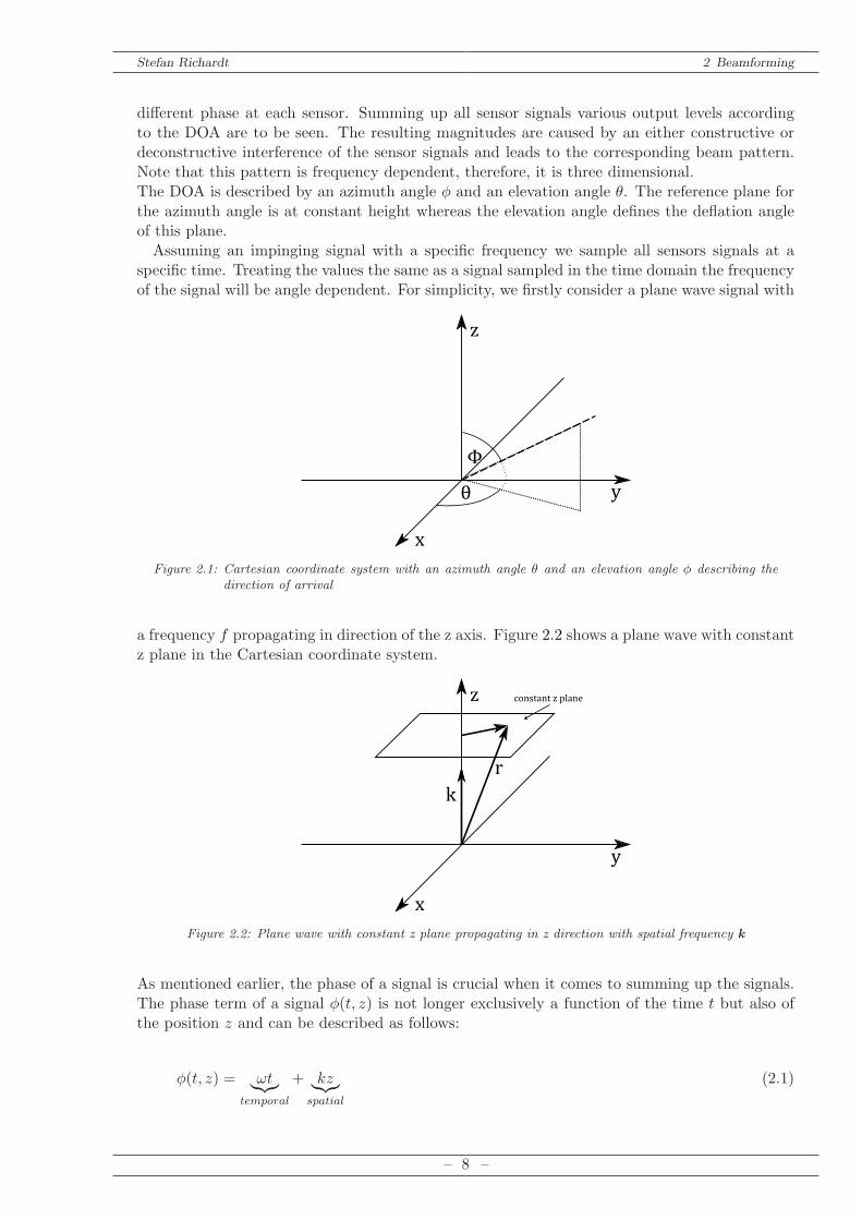
different phase at each sensor. Summing up all sensor signals various output levels accordingto the DOA are to be seen. The resulting magnitudes are caused by an either constructive ordeconstructive interference of the sensor signals and leads to the corresponding beam pattern.Note that this pattern is frequency dependent, therefore, it is three dimensional.The DOA is described by an azimuth angle φ and an elevation angle θ. The reference plane forthe azimuth angle is at constant height whereas the elevation angle defines the deflation angleof this plane.Assuming an impinging signal with a specific frequency we sample all sensors signals at a
specific time. Treating the values the same as a signal sampled in the time domain the frequencyof the signal will be angle dependent. For simplicity, we firstly consider a plane wave signal with
x
y
z
θ
Φ
Figure 2.1: Cartesian coordinate system with an azimuth angle θ and an elevation angle φ describing thedirection of arrival
a frequency f propagating in direction of the z axis. Figure 2.2 shows a plane wave with constantz plane in the Cartesian coordinate system.
x
y
z
k
r
constantzplane
Figure 2.2: Plane wave with constant z plane propagating in z direction with spatial frequency k
As mentioned earlier, the phase of a signal is crucial when it comes to summing up the signals.The phase term of a signal φ(t, z) is not longer exclusively a function of the time t but also ofthe position z and can be described as follows:
φ(t, z) = ωt︸︷︷︸
temporal
+ kz︸︷︷︸
spatial
(2.1)
– 8 –
Stefan Richardt 2 Beamforming
In order to express the position term we need to introduce the wavenumber k:
k =ω
c=
2πf
c=
2π
λ(2.2)
k contains the temporal, angular frequency ω respectively the signal frequency f . Additionally,λ denotes the resulting wavelength and c is the propagation speed in a particular medium. FormEquation (2.1) it can be seen that ω is used as a fixed factor for the time t whereas k is used asfixed factor for the position z. As ω is called temporal frequency it is common to name k thespatial frequency. Instead of giving the number of periods per seconds k represents the numberof periods per meter. Denote that k is also dependent on the signal frequency f . For a moredetailed and well illustrated explanation of the wavenumber k see [Williams, 1999].Assuming to shift the observation point along the z axis the phase changes according to thespacial frequency k whereby the phase shift is the same for all points in this plane.Unlike the temporal frequency ω the spacial frequency k is three dimensional and points inthe directions of the propagating wave. In Cartesian coordinates it can be denoted as a threedimensional vector:
k = [kx ky kz]T (2.3)
The length can be calculated as follows:
k =√
k2x + k2y + k2z (2.4)
In the particular case shown in Figure 2.2 k consits of kx = ky = 0 and kz = k. Defining theunity vector z along the z axis:
z = [0 0 1]T (2.5)
leads to:
k = kz (2.6)
If we want to show the relation between k and f we need to refer to Equation (2.2).Within the next steps we describe any point in a 3D space. For that reason we introduce r, whichdirectly gives the coordinates in the Cartesian system. Using k we are now able to formulate thephase φ(t, r) as function of r, enabling to give the phase of a signal at every possible position ina room. Therefore, we rewrite Equation (2.1):
φ(t, r) = ωt︸︷︷︸
temporal
+ kT r︸︷︷︸
spatial
(2.7)
with:
r = [rx ry rz]T (2.8)
In order to gain more generality we replace the coordinates by the angles θ and φ. As we assume
– 9 –
Stefan Richardt 2 Beamforming
plane waves, analogous to the far field assumption, there is no need to include the distance fromthe source to the sensor. Finally we are able to determine a time independent phase term, whichis a function of the DOA as only the angles of an impinging signal are significant.
k =
kxkykz
= k
sin θ cos φsin θ sin φ
cos θ
(2.9)
Applying Equation (2.8) and Equation (2.9) in Equation (2.7) and focusing on the time inde-pendent phase term we obtain:
kT r = sin θ cos φ rx + sin θ sin φ ry + cos θ rz (2.10)
Thus, we have expressed the phase of a signal as function of time and DOA. As we are able todescribe the phase of a signal at every point in 3D space we want to utilize the spatial phaseshift. Placing sensors at different locations constitutes an array and in further consequence abeamformer.
2.2 Problem description, Assumptions and Specifications
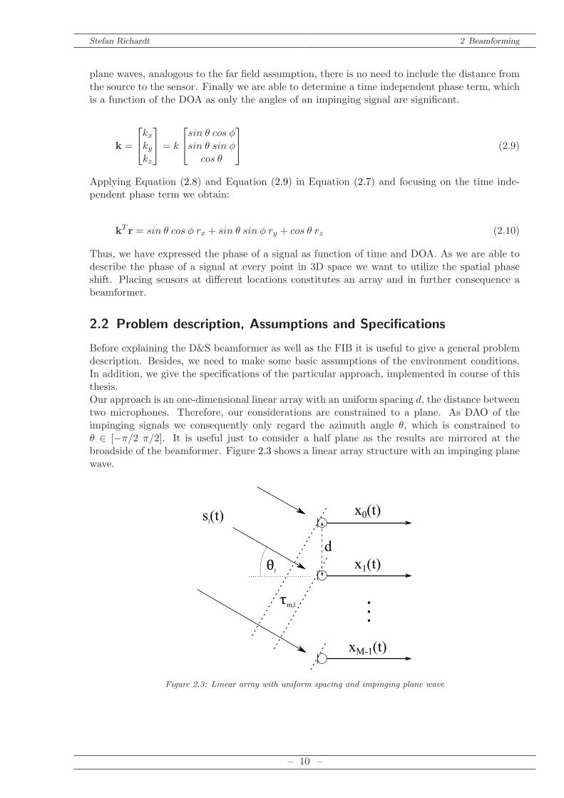
Before explaining the D&S beamformer as well as the FIB it is useful to give a general problemdescription. Besides, we need to make some basic assumptions of the environment conditions.In addition, we give the specifications of the particular approach, implemented in course of thisthesis.Our approach is an one-dimensional linear array with an uniform spacing d, the distance betweentwo microphones. Therefore, our considerations are constrained to a plane. As DAO of theimpinging signals we consequently only regard the azimuth angle θ, which is constrained toθ ∈ [−π/2 π/2]. It is useful just to consider a half plane as the results are mirrored at thebroadside of the beamformer. Figure 2.3 shows a linear array structure with an impinging planewave.
sl(t) x0(t)
x1(t)
xM-1(t)
τm,l
θl
d
Figure 2.3: Linear array with uniform spacing and impinging plane wave
– 10 –
Stefan Richardt 2 Beamforming
sl . . . l-th source signal
L . . . number of sources
xM . . . x-th microphone signal
M . . . number of microphones
d . . . distance between microphones
θl . . . DOA / angle of impinging signal of l-th source
τm,l . . . time delay to reference micrphone
We suppose that sl(t) is the l-th impinging signal with l = 0, 1, . . . , L − 1 where L is thenumber of source signals. According to each of the source signals we describe the directionof arrival by θl. Basically our model contains M sensors, which provide the received signalsx0(t), x1(t), . . . , xM−1(t). We consider the zeroth sensor to be our reference. Hence, we areable to define τm,l as time delay from the reference sensor to the m-th sensor according to thel-th source. The delay τm,l depends on the angle of the impinging signal θl and the distanceof the m-th sensor form the reference. As we have an uniform sensor distribution with a fixeddistance d between the microphones the delay τm,l can be considered as:
τm,l = sin(φl)m · dc
(2.11)
The wave propagation speed of sound waves in air is:
c ≈ 340m
s(2.12)
In general the signal at the m-th sensor can be described by:
xm(t) = αms(t− tl − τm,l) + υn(t) (2.13)
with:
αm . . . attenuation factor of microphone m
tl . . . time delay from the source l to the reference sensor
υn(t) . . . uncorrelated noise
Ideally the attenuation factor αm is the same for all microphones as we assume plane wavesrespectively far field conditions. Apart from the additional noise we basically obtain the samesignal s(t) whose differences in terms of time delay are exclusively determined by τm,l. The noiseυn(t) is caused by the microphones themselves and by the Analogue Digital (AD) converters. Itis supposed to be uncorrelated.Furthermore, we want to introduce a signal model for a multipath environment. In general,reflections in a room can be described as attenuated and delayed versions of the original signal.All basic assumptions remain. Based on Equation (2.13) we add a term for a certain number of
– 11 –
Stefan Richardt 2 Beamforming
reflections:
xm(t) = αms(t− tl − τm,l) + υn(t) +R∑
r=1
αm,rs(t− tl,r − τm,l,r) (2.14)
with:
R . . . Number of reflections
tl,r . . . time delay of the r-th path from source l to the reference sensor
αm,r . . . attenuation factor of the m-th microphone according to the r-th path
We assume that all array sensors have the same characteristics. This means that the varietiesof gains and frequency responses in terms of magnitude and phase should ideally be zero. It isalso supposed that the sensors are omni directional meaning their responses to any impingingsignals are independent of their DOA. As we deal exclusively with acoustic signals the usedmicrophones need to provide a capsule with an omni directional directivity pattern.As mentioned earlier we assume that all impinging signals are plane waves. Depending on thearray aperture and the distance between microphones and source this assumption can not alwayscomplied. A more detailed discussion can be found in Chapter 7.3.
2.3 Delay and Sum Beamformer
The D&S beamformer can be described by a general model of a narrow band beamformer. AD&S beamformer normally consists of two stages.The first stage delays the sensor signals whereas the seconds sums up all the signals. Without
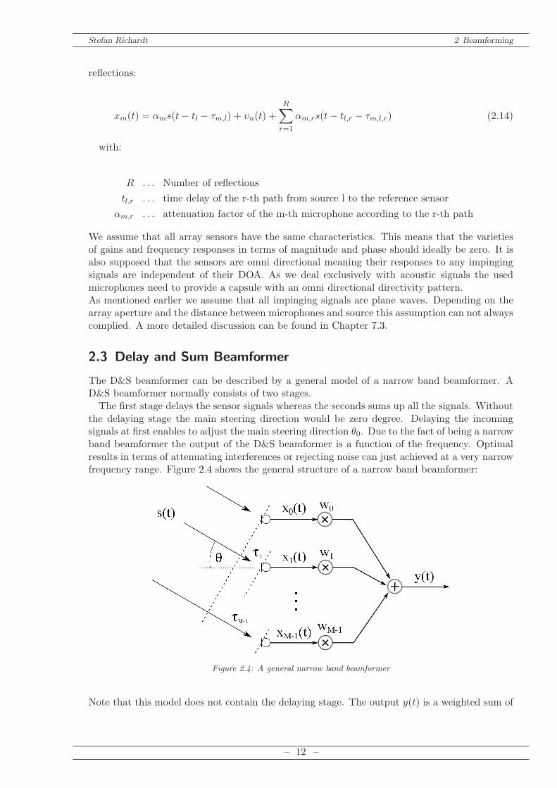
the delaying stage the main steering direction would be zero degree. Delaying the incomingsignals at first enables to adjust the main steering direction θ0. Due to the fact of being a narrowband beamformer the output of the D&S beamformer is a function of the frequency. Optimalresults in terms of attenuating interferences or rejecting noise can just achieved at a very narrowfrequency range. Figure 2.4 shows the general structure of a narrow band beamformer:
s(t) x0(t)
x1(t)
xM-1(t)
τ1
τM-1
θ
Figure 2.4: A general narrow band beamformer
Note that this model does not contain the delaying stage. The output y(t) is a weighted sum of
– 12 –
Stefan Richardt 2 Beamforming
the sensor signals, whereas wm is the weighting factor according to the m-th signal:
y(t) =M−1∑
m=0
xm(t)wm (2.15)
In order to describe the frequency response of the beamformer in the following we define thecomplex sensor signal x(t) for one source with a DOA angle θ. We assume a signal with theangular frequency ω and zero phase shift at the reference sensor:
x0(t) = ejωt (2.16)
Hence, the signal at all sensors can be described by utilizing τm introduced in Equation (2.11):
xm(t) = ejω(t−τm) = ejωte−jωτm (2.17)
Applying Equation (2.17) to Equation (2.15) leads to:
y(t) = ejωtM−1∑
m=0
e−jωτmwm (2.18)
Excluding the temporal part we are able to define the beampattern P (ω, θ):
P (ω, θ) =M−1∑
m=0
e−jωτmwm (2.19)
The beampattern is a function of the temporal angular signal frequency ω and the DAO angleθ, contained by the time delay τm. Dealing with a discrete aperture brings along the problemof spatial aliasing. Comparable to temporal aliasing a certain frequency of the incoming signalshould not be exceeded. The Nyquist criterion is also valid in terms of spatial sampling. For amore detailed explanation and several examples concerning this problem please see [Williams,1999] and [Dollfuß, 2010]. We consider λ to be the smallest possible wavelength of the sourcesignal. According to this we can set a suitable distance d.
d =λmin
2(2.20)
Defining the weighting vector w and the steering vector d(ω, θ) enables to rewrite Equa-tion(2.19) in vector form:
P (ω, θ) = wT d(ω, θ) (2.21)
with:
w = [ w0 w1 w2 . . . wM−1 ]T (2.22)
– 13 –
Stefan Richardt 2 Beamforming
and:
d(ω, θ) = [ 1 ejωτ1 ejωτ2 . . . ejωτM−1 ]T (2.23)
The weighting vector w can be seen as spacial window function. Regarding parameters suchas main beam width or side lobe attenuation various spatial windows are possible. The verysimplest case is the D&S beamformer with:
w =1
M[ 1 1 . . . 1 ]T (2.24)
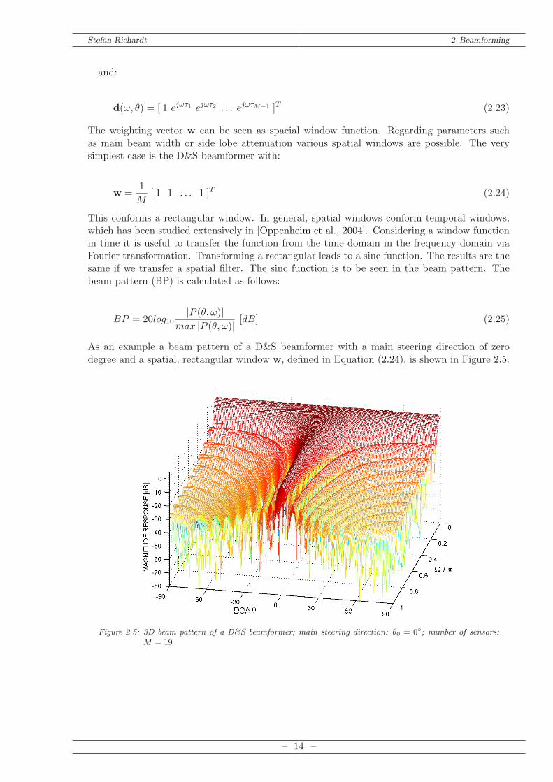
This conforms a rectangular window. In general, spatial windows conform temporal windows,which has been studied extensively in [Oppenheim et al., 2004]. Considering a window functionin time it is useful to transfer the function from the time domain in the frequency domain viaFourier transformation. Transforming a rectangular leads to a sinc function. The results are thesame if we transfer a spatial filter. The sinc function is to be seen in the beam pattern. Thebeam pattern (BP) is calculated as follows:
BP = 20log10|P (θ, ω)|
max |P (θ, ω)| [dB] (2.25)
As an example a beam pattern of a D&S beamformer with a main steering direction of zerodegree and a spatial, rectangular window w, defined in Equation (2.24), is shown in Figure 2.5.
Figure 2.5: 3D beam pattern of a D&S beamformer; main steering direction: θ0 = 0; number of sensors:M = 19
– 14 –
Stefan Richardt 2 Beamforming
2.4 Frequency Invariant Beamformer
Unlike the D&S beamformer the Frequency Invariant Beamforming (FIB) technique is an arraydesign for wideband signals. Ideally, the response is exclusively a function of the DOA angle ofthe impinging signal and, thus, not frequency dependent. However, it is practically not possibleto design a frequency invariant beamformer valid for the whole spectrum. Consequently, thesignals have to be restricted to the valid range.Regarding a FIB also known as Filter and Sum (F&S) beamformer every sensor signal xm(t)
is convoluted by a Finite Impulse Response (FIR) filter. The aim is to design a fixed set offilter coefficients (non-adaptive) in order to achieve frequency independence. Furthermore, thedelaying stage is implemented by the filters, hence, a set of filter coefficients for each steeringdirection is required.The method which is used here is proposed in [Liu and Weiss, 2008], [Sekiguchi and Kara-
sawa, 2000]. To achieve frequency-independence we exploit the Fourier transform. The spatio-temporal distribution P (ω, θ) of a 1D array, which is dependent on the DOA angle θ of theimpinging signal and its frequency ω, can be characterized by a two dimensional discrete Fouriertransformation. With the help of specific substitutions we are able to design a beam patterndependent on normalized angular frequencies such as P (Ω1,Ω2). If we can define an appropriatebeam pattern it is possible to apply the 2D inverse Fourier transformation to gain the desiredfilter coefficients. A detailed description of the process and the filter design is given below.
2.4.1 Design Procedure
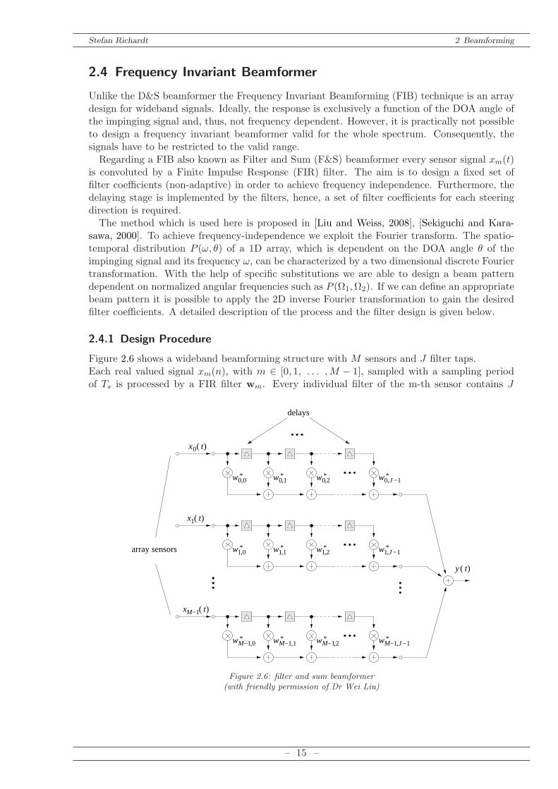
Figure 2.6 shows a wideband beamforming structure with M sensors and J filter taps.Each real valued signal xm(n), with m ∈ [0, 1, . . . ,M − 1], sampled with a sampling periodof Ts is processed by a FIR filter wm. Every individual filter of the m-th sensor contains J
,
,2
,0
,
,
,2,1,0
,1,0
,2,1
array sensors
*
*
*
delays
**
*
* *
*
*
**
(
M−1 )( tx
M−1 M−1 M−1 M−1
)y t
)( tx0
)( t1x
w0 w0
w1 w1
w w w w
w
w1
0 −1J
J −1
−1J
w1
w0
Figure 2.6: filter and sum beamformer(with friendly permission of Dr Wei Liu)
– 15 –
Stefan Richardt 2 Beamforming
coefficients wm,j , which are also claimed to be real. These coefficients need to be calculated.The acquired 2D filter exceeds to a 3D filter as a 2D set for each main steering direction θ0 has tobe calculated. Criteria for the performance of these filters are for example side lobe attenuation,the valid frequency range but also error robustness and stability [Pape, 2005].In order to avoid aliasing in the time domain the sampling frequency fs should be larger
then twice of the maximum frequency of interest fmax. To prevent spatial aliasing the distancebetween two microphones d should be less then half of the minimal wavelength of interest λmin
according to the maximal frequency. Finally we can denote two simple requirements:
2fmax < fs =1
Ts(2.26)
λmin =c
fmax< 2d (2.27)
Combining both conditions we set the sensor spacing d pursuant to the maximal signal frequency:
d =λmin
2= cTs (2.28)
According to the signal model for a linear, equally spaced array in chapter 1.2 the beam responseP (ω, θ) from Equation (2.19) can be exceeded to:
P (ω, θ) =M−1∑
m=0
J−1∑
k=0
wm,k · e−jmωτ · e−jkωTs (2.29)
whereas the time delay between two adjacent microphones is:
τ = sinθ · dc
(2.30)
With consideration of the assumption being made in Equation (2.28) we define a constant µ,however, we are instantly able to simplify the problem:
µ =d
cTs=
cTs
cTs= 1 (2.31)
As a result we can rewrite Equation (2.29) as follows:
P (Ω, θ) =M−1∑
m=0
J−1∑
k=0
wm,k · e−jmµΩ sinθ · e−jkΩ (2.32)
with the normalized angular frequency:
Ω = ωTs (2.33)
The next step is to apply a spectral transformation. To achieve a beam pattern P (Ω1,Ω2),which is only dependent on normalized angular frequencies, we substitute as follows:
– 16 –
Stefan Richardt 2 Beamforming
Ω1 = µΩsinθ = Ωsinθ (2.34)
Ω2 = Ω (2.35)
which yields to:
P (Ω1,Ω2) =M−1∑
m=0
J−1∑
k=0
wm,k · e−jmΩ2 · e−jkΩ1 (2.36)
Ω1 represents the spatial normalized angular frequency, while Ω2 stands for the temporal nor-malized angular frequency. Denote that the simplification of µ = 1 which yields to a much easierequation is only possible as we set d according to the sampling frequency fs as already donein Equation (2.28). Regarding the relationship: Ω1 = Ω2 sinθ it can easily be seen that theimpinging signals must comply the following expression:
|Ω1| ≤ |Ω2| (2.37)
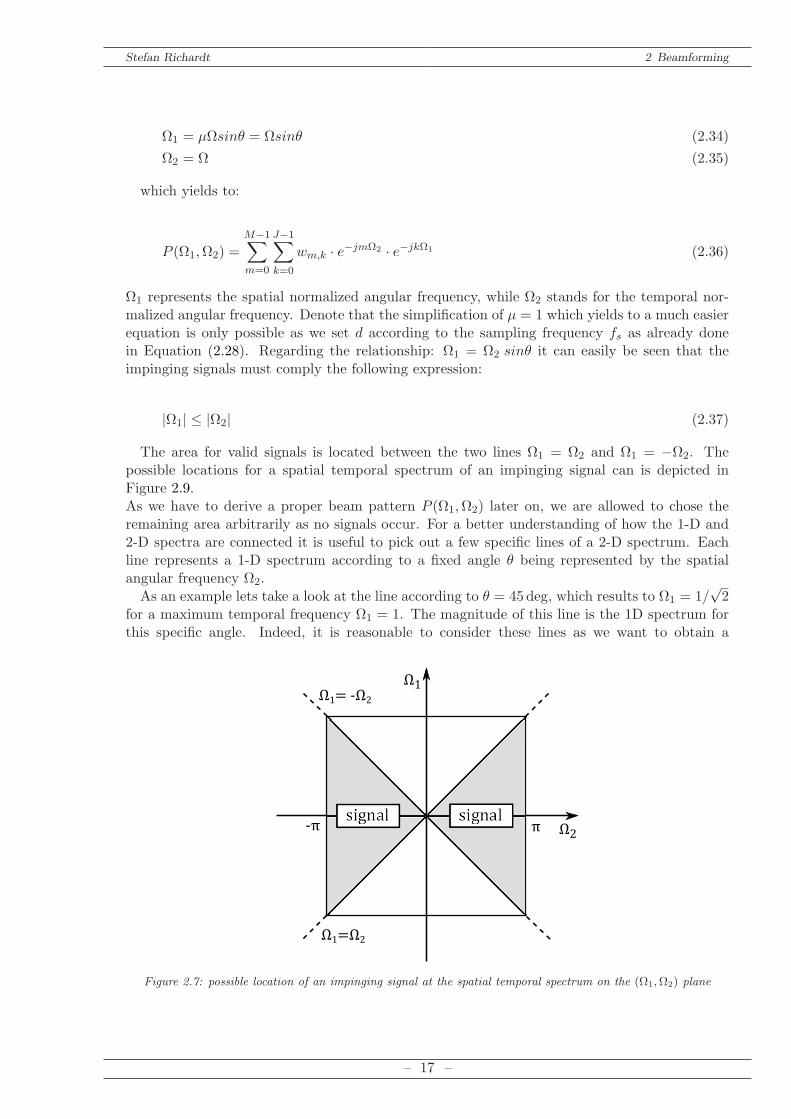
The area for valid signals is located between the two lines Ω1 = Ω2 and Ω1 = −Ω2. Thepossible locations for a spatial temporal spectrum of an impinging signal can is depicted inFigure 2.9.As we have to derive a proper beam pattern P (Ω1,Ω2) later on, we are allowed to chose theremaining area arbitrarily as no signals occur. For a better understanding of how the 1-D and2-D spectra are connected it is useful to pick out a few specific lines of a 2-D spectrum. Eachline represents a 1-D spectrum according to a fixed angle θ being represented by the spatialangular frequency Ω2.As an example lets take a look at the line according to θ = 45deg, which results to Ω1 = 1/
√2
for a maximum temporal frequency Ω1 = 1. The magnitude of this line is the 1D spectrum forthis specific angle. Indeed, it is reasonable to consider these lines as we want to obtain a
Ω2-π π
Ω1=Ω2
Ω1Ω1=-Ω2
Figure 2.7: possible location of an impinging signal at the spatial temporal spectrum on the (Ω1,Ω2) plane
– 17 –
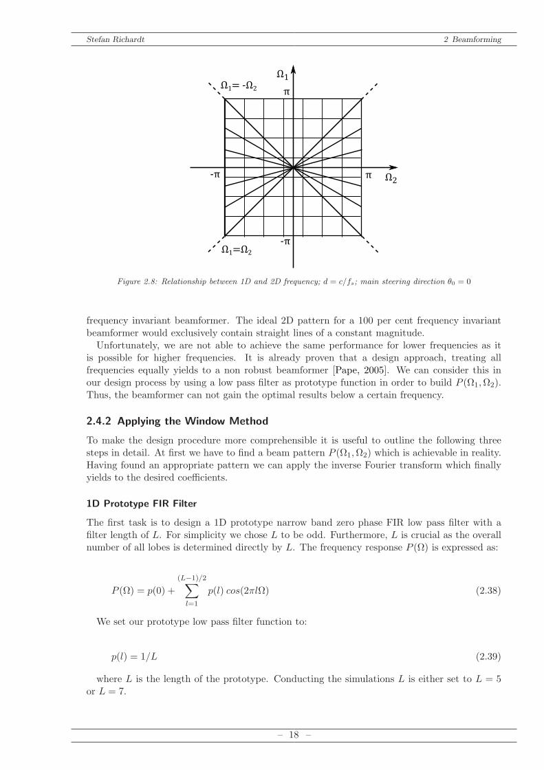
Stefan Richardt 2 Beamforming
Ω2-π π
Ω1=Ω2
Ω1=-Ω2
Ω1
π
-π
Figure 2.8: Relationship between 1D and 2D frequency; d = c/fs; main steering direction θ0 = 0
frequency invariant beamformer. The ideal 2D pattern for a 100 per cent frequency invariantbeamformer would exclusively contain straight lines of a constant magnitude.Unfortunately, we are not able to achieve the same performance for lower frequencies as it
is possible for higher frequencies. It is already proven that a design approach, treating allfrequencies equally yields to a non robust beamformer [Pape, 2005]. We can consider this inour design process by using a low pass filter as prototype function in order to build P (Ω1,Ω2).Thus, the beamformer can not gain the optimal results below a certain frequency.
2.4.2 Applying the Window Method
To make the design procedure more comprehensible it is useful to outline the following threesteps in detail. At first we have to find a beam pattern P (Ω1,Ω2) which is achievable in reality.Having found an appropriate pattern we can apply the inverse Fourier transform which finallyyields to the desired coefficients.
1D Prototype FIR Filter
The first task is to design a 1D prototype narrow band zero phase FIR low pass filter with afilter length of L. For simplicity we chose L to be odd. Furthermore, L is crucial as the overallnumber of all lobes is determined directly by L. The frequency response P (Ω) is expressed as:
P (Ω) = p(0) +
(L−1)/2∑
l=1
p(l) cos(2πlΩ) (2.38)
We set our prototype low pass filter function to:
p(l) = 1/L (2.39)
where L is the length of the prototype. Conducting the simulations L is either set to L = 5or L = 7.
– 18 –
Stefan Richardt 2 Beamforming
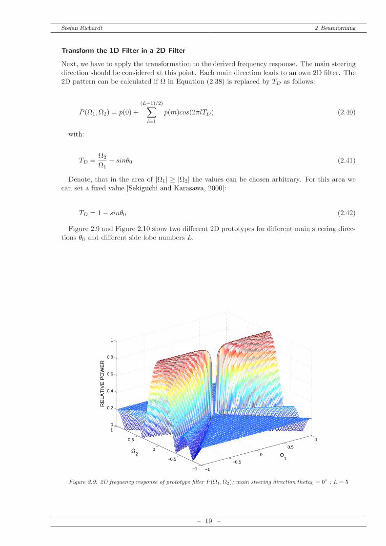
Transform the 1D Filter in a 2D Filter
Next, we have to apply the transformation to the derived frequency response. The main steeringdirection should be considered at this point. Each main direction leads to an own 2D filter. The2D pattern can be calculated if Ω in Equation (2.38) is replaced by TD as follows:
P (Ω1,Ω2) = p(0) +
(L−1)/2)∑
l=1
p(m)cos(2πlTD) (2.40)
with:
TD =Ω2
Ω1− sinθ0 (2.41)
Denote, that in the area of |Ω1| ≥ |Ω2| the values can be chosen arbitrary. For this area wecan set a fixed value [Sekiguchi and Karasawa, 2000]:
TD = 1− sinθ0 (2.42)
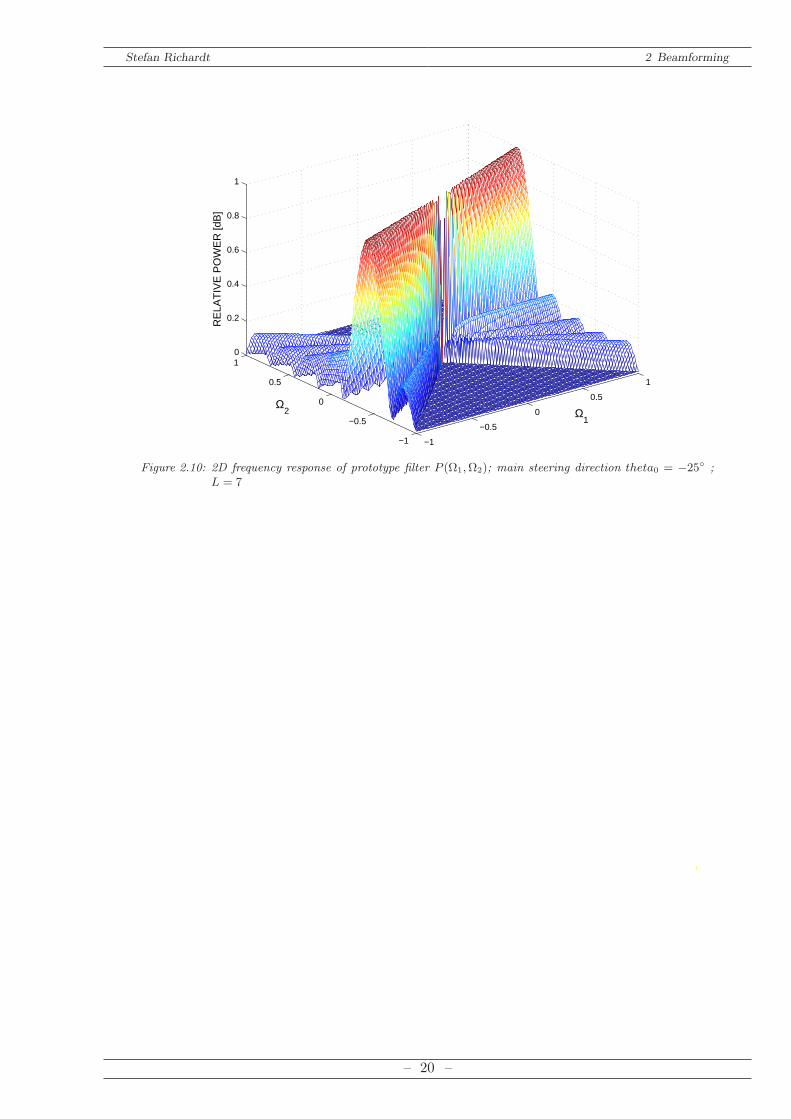
Figure 2.9 and Figure 2.10 show two different 2D prototypes for different main steering direc-tions θ0 and different side lobe numbers L.
−1
−0.5
0
0.5
1
−1
−0.5
0
0.5
10
0.2
0.4
0.6
0.8
1
Ω1
Ω2
RE
LAT
IVE
PO
WE
R
Figure 2.9: 2D frequency response of prototype filter P (Ω1,Ω2); main steering direction theta0 = 0 ; L = 5
– 19 –
Stefan Richardt 2 Beamforming
−1
−0.5
0
0.5
1
−1
−0.5
0
0.5
10
0.2
0.4
0.6
0.8
1
Ω1
Ω2
RE
LAT
IVE
PO
WE
R [d
B]
Figure 2.10: 2D frequency response of prototype filter P (Ω1,Ω2); main steering direction theta0 = −25 ;L = 7
– 20 –
Stefan Richardt 2 Beamforming
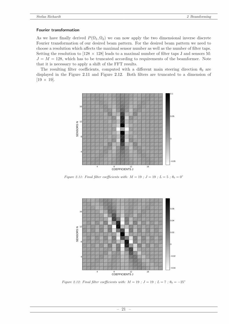
Fourier transformation
As we have finally derived P (Ω1,Ω2) we can now apply the two dimensional inverse discreteFourier transformation of our desired beam pattern. For the desired beam pattern we need tochoose a resolution which affects the maximal sensor number as well as the number of filter taps.Setting the resolution to [128 × 128] leads to a maximal number of filter taps J and sensors M:J = M = 128, which has to be truncated according to requirements of the beamformer. Notethat it is necessary to apply a shift of the FFT results.The resulting filter coefficients, computed with a different main steering direction θ0 are
displayed in the Figure 2.11 and Figure 2.12. Both filters are truncated to a dimension of[19 × 19].
4 8 12 16
4
8
12
16
COEFFICIENTS J
SE
NS
OR
S N
−0.05
0
0.05
0.1
Figure 2.11: Final filter coefficients with: M = 19 ; J = 19 ; L = 5 ; θ0 = 0
4 8 12 16
4
8
12
16
COEFFICIENTS J
SE
NS
OR
S N
−0.04
−0.02
0
0.02
0.04
0.06
Figure 2.12: Final filter coefficients with: M = 19 ; J = 19 ; L = 7 ; θ0 = −25
– 21 –
Stefan Richardt 2 Beamforming
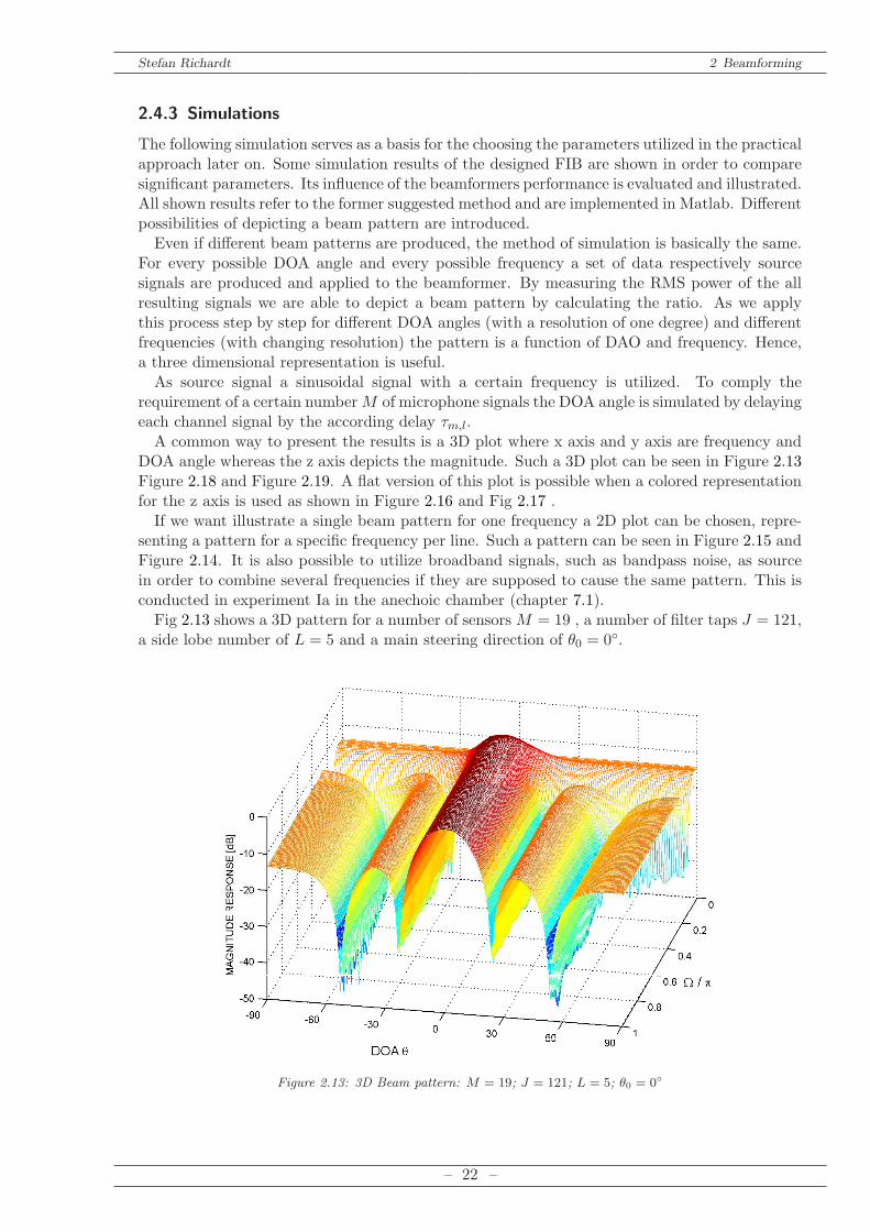
2.4.3 Simulations
The following simulation serves as a basis for the choosing the parameters utilized in the practicalapproach later on. Some simulation results of the designed FIB are shown in order to comparesignificant parameters. Its influence of the beamformers performance is evaluated and illustrated.All shown results refer to the former suggested method and are implemented in Matlab. Differentpossibilities of depicting a beam pattern are introduced.Even if different beam patterns are produced, the method of simulation is basically the same.
For every possible DOA angle and every possible frequency a set of data respectively sourcesignals are produced and applied to the beamformer. By measuring the RMS power of the allresulting signals we are able to depict a beam pattern by calculating the ratio. As we applythis process step by step for different DOA angles (with a resolution of one degree) and differentfrequencies (with changing resolution) the pattern is a function of DAO and frequency. Hence,a three dimensional representation is useful.As source signal a sinusoidal signal with a certain frequency is utilized. To comply the
requirement of a certain numberM of microphone signals the DOA angle is simulated by delayingeach channel signal by the according delay τm,l.A common way to present the results is a 3D plot where x axis and y axis are frequency and
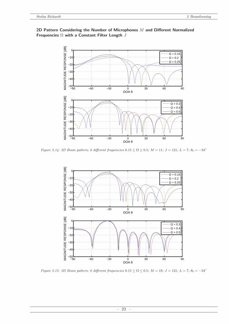
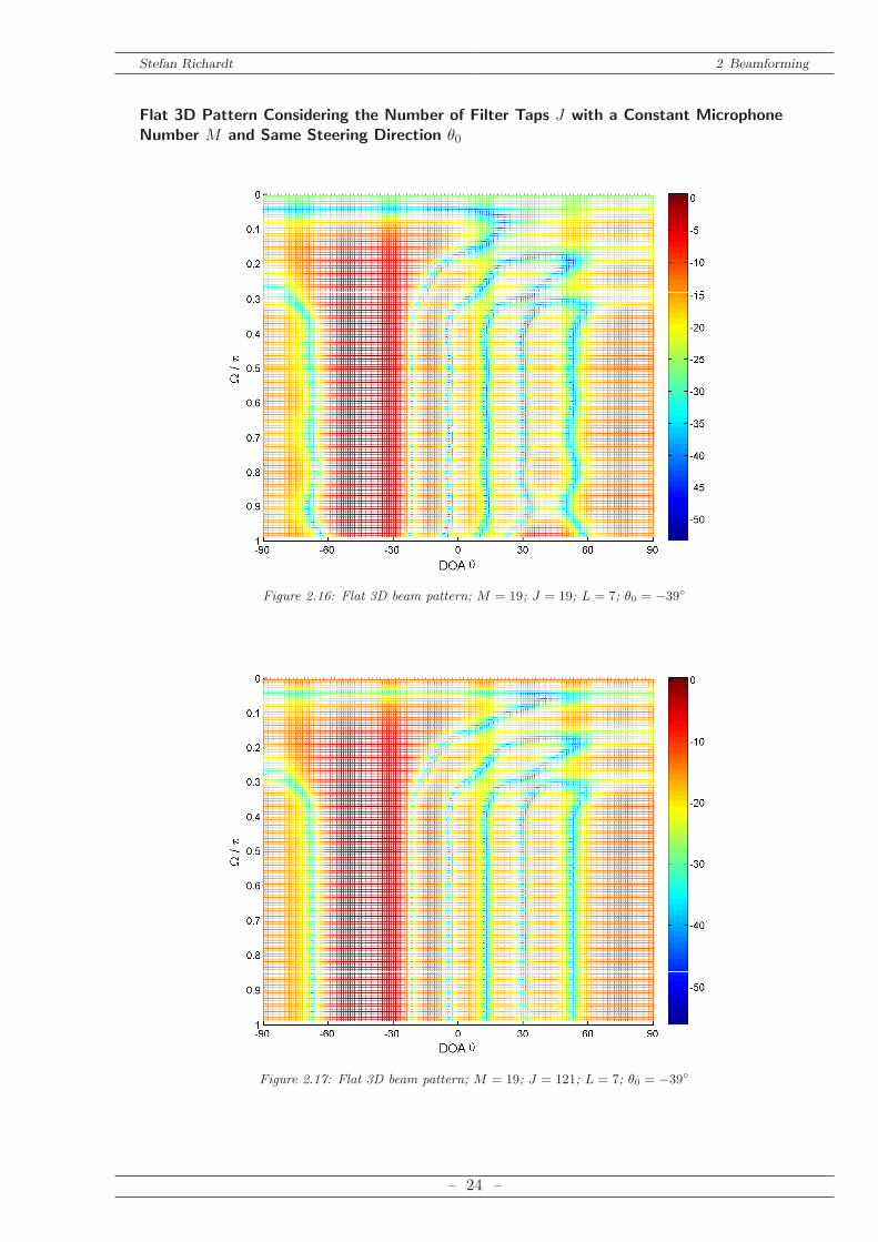
DOA angle whereas the z axis depicts the magnitude. Such a 3D plot can be seen in Figure 2.13Figure 2.18 and Figure 2.19. A flat version of this plot is possible when a colored representationfor the z axis is used as shown in Figure 2.16 and Fig 2.17 .If we want illustrate a single beam pattern for one frequency a 2D plot can be chosen, repre-
senting a pattern for a specific frequency per line. Such a pattern can be seen in Figure 2.15 andFigure 2.14. It is also possible to utilize broadband signals, such as bandpass noise, as sourcein order to combine several frequencies if they are supposed to cause the same pattern. This isconducted in experiment Ia in the anechoic chamber (chapter 7.1).Fig 2.13 shows a 3D pattern for a number of sensors M = 19 , a number of filter taps J = 121,
a side lobe number of L = 5 and a main steering direction of θ0 = 0.
Figure 2.13: 3D Beam pattern: M = 19; J = 121; L = 5; θ0 = 0
– 22 –
Stefan Richardt 2 Beamforming
2D Pattern Considering the Number of Microphones M and Different Normalized
Frequencies Ω with a Constant Filter Length J
−90 −60 −30 0 30 60 90−50
−40
−30
−20
−10
0
DOA θ
MA
GN
ITU
DE
RE
SP
ON
SE
[dB
]
Ω = 0.15Ω = 0.2Ω = 0.25
−90 −60 −30 0 30 60 90−50
−40
−30
−20
−10
0
DOA θ
MA
GN
ITU
DE
RE
SP
ON
SE
[dB
]
Ω = 0.3Ω = 0.4Ω = 0.5
Figure 2.14: 2D Beam pattern; 6 different frequencies 0.15 ≤ Ω ≤ 0.5; M = 11; J = 121; L = 7; θ0 = −34
−90 −60 −30 0 30 60 90−50
−40
−30
−20
−10
0
DOA θ
MA
GN
ITU
DE
RE
SP
ON
SE
[dB
]
Ω = 0.15Ω = 0.2Ω = 0.25
−90 −60 −30 0 30 60 90−50
−40
−30
−20
−10
0
DOA θ
MA
GN
ITU
DE
RE
SP
ON
SE
[dB
]
Ω = 0.3Ω = 0.4Ω = 0.5
Figure 2.15: 2D Beam pattern; 6 different frequencies 0.15 ≤ Ω ≤ 0.5; M = 19; J = 121; L = 7; θ0 = −34
– 23 –
Stefan Richardt 2 Beamforming
Flat 3D Pattern Considering the Number of Filter Taps J with a Constant Microphone
Number M and Same Steering Direction θ0
Figure 2.16: Flat 3D beam pattern; M = 19; J = 19; L = 7; θ0 = −39
Figure 2.17: Flat 3D beam pattern; M = 19; J = 121; L = 7; θ0 = −39
– 24 –
Stefan Richardt 2 Beamforming
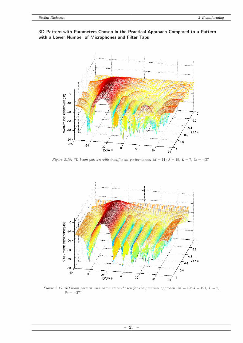
3D Pattern with Parameters Chosen in the Practical Approach Compared to a Pattern
with a Lower Number of Microphones and Filter Taps
Figure 2.18: 3D beam pattern with insufficient performance: M = 11; J = 19; L = 7; θ0 = −37
Figure 2.19: 3D beam pattern with parameters chosen for the practical approach: M = 19; J = 121; L = 7;θ0 = −37
– 25 –
Stefan Richardt 2 Beamforming
2.4.4 Conclusion
The former results illustrate the impact of three parameters:
Filter length of the 1D prototype L . . . respectively the side lobe number L− 1
Number of microphones M
Number of filter taps J
As already mentioned in Chapter 2.4.2 the choice of the filter length L of the 1D prototypedirectly determines the number of side lobes. A certain number is needed as we want to cancelseveral interfering signals. This will be discussed later in Chapter 4 as well as in Chapter 8.2.3.For now, a number of L = 7 is chosen.The Number of microphones M is evaluated in Figure 2.14 and Figure 2.15. It can be seen
that an increasing number of microphonesM extends the frequency range where the beamformeris working frequency independently. Hence, the maximal, practically available number is chosen:M = 19.The Number of filter taps J is considered in Figure 2.16 and Figure 2.17. It is shown that
a smaller number of filter taps J has an impact of the beamformers performance in the validfrequency range as the main lobe as well as some side lobes are distorted. Therefore, a sufficientlyhigh number of filter taps is chosen: J = 121.Concluding with Figure 2.19 a simulation with the finally chosen parameters is conducted:
L = 7, M = 19 and J = 121.
2.4.5 Fractional Delay
When dealing with beamforming the topic of delaying signals is important. For example, it ispossible to change the steering direction of a beamformer by adding appropriate delays (Chapter2.3). Furthermore, it is essential for any kind of simulation. A filter delaying a signal by aninteger number of samples is defined as follows:
h[n] = δ[n− n0] (2.43)
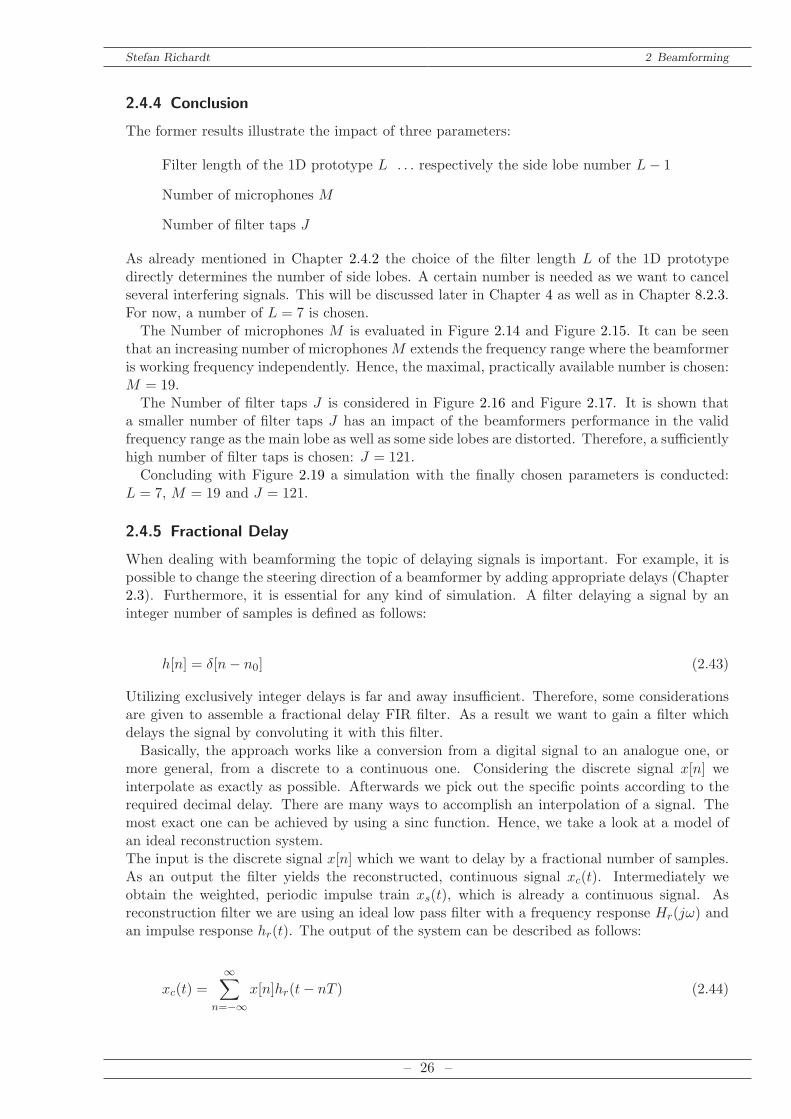
Utilizing exclusively integer delays is far and away insufficient. Therefore, some considerationsare given to assemble a fractional delay FIR filter. As a result we want to gain a filter whichdelays the signal by convoluting it with this filter.Basically, the approach works like a conversion from a digital signal to an analogue one, or
more general, from a discrete to a continuous one. Considering the discrete signal x[n] weinterpolate as exactly as possible. Afterwards we pick out the specific points according to therequired decimal delay. There are many ways to accomplish an interpolation of a signal. Themost exact one can be achieved by using a sinc function. Hence, we take a look at a model ofan ideal reconstruction system.The input is the discrete signal x[n] which we want to delay by a fractional number of samples.As an output the filter yields the reconstructed, continuous signal xc(t). Intermediately weobtain the weighted, periodic impulse train xs(t), which is already a continuous signal. Asreconstruction filter we are using an ideal low pass filter with a frequency response Hr(jω) andan impulse response hr(t). The output of the system can be described as follows:
xc(t) =∞∑
n=−∞
x[n]hr(t− nT ) (2.44)
– 26 –
Stefan Richardt 2 Beamforming
Convert from
sequence to
impulse train
Ideal
reconstruction
filter
Hr(jw) xc(t)xs(t)x[n]
Sampling
period T
n0 1 2 3 4-1-2-3-4
x[n]
t
xc(t)
0 2--2
xs(t)
Figure 2.20: Ideal reconstruction system with discrete input x[n], weighted impulse train xs(t) and continuoussignal xc(t)
t
hr(t)1
0 2--2 3-3 4-4
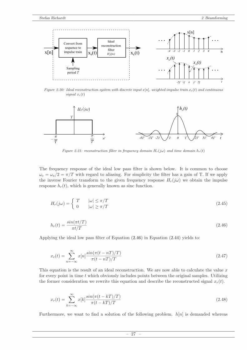
Figure 2.21: reconstruction filter in frequency domain Hr(jω) and time domain hr(t)
The frequency response of the ideal low pass filter is shown below. It is common to chooseωc = ωs/2 = π/T with regard to aliasing. For simplicity the filter has a gain of T. If we applythe inverse Fourier transform to the given frequency response Hr(jω) we obtain the impulseresponse hr(t), which is generally known as sinc function.
Hr(jω) =
T |ω| ≤ π/T
0 |ω| ≥ π/T(2.45)
hr(t) =sin(πt/T )
πt/T(2.46)
Applying the ideal low pass filter of Equation (2.46) in Equation (2.44) yields to:
xc(t) =∞∑
n=−∞
x[n]sin(π(t− nT )/T )
π(t− nT )/T(2.47)
This equation is the result of an ideal reconstruction. We are now able to calculate the value xfor every point in time t which obviously includes points between the original samples. Utilizingthe former consideration we rewrite this equation and describe the reconstructed signal xr(t).
xr(t) =
∞∑
k=−∞
x[k]sin(π(t− kT )/T )
π(t− kT )/T(2.48)
Furthermore, we want to find a solution of the following problem. h[n] is demanded whereas
– 27 –
Stefan Richardt 2 Beamforming
y[n] shall be the final fractionally delayed signal.
y[n] = x[n] ∗ h[n] (2.49)
If we delay xr(t) it corresponds to y[n]. To fit this requirement we delay xr(t) about αTwhereas α is the fractional delay factor with 0 ≤ α ≤ 1.
xr(t− αT ) =∞∑
k=−∞
x[k]sin(π(t− αT − kT )/T )
π(t− αT − kT )/T(2.50)
With the definition of t = nT we finally replace xr(t− αT ) by y[n].
y[n] = xc(t− αT )|t=nT (2.51)
After a few simplifications we accomplish our calculations. As a result we obtain h[n].
y[n] =∞∑
k=−∞
x[k]sin(π(nT − αT − kT )/T )
π(nT − αT − kT )/T(2.52)
y[n] =
∞∑
k=−∞
x[k]sin(π(n− α− k))
π(n− α− k)(2.53)
y[n] = x[n] ∗ h[n] (2.54)
h[n] =sin(π(n− α))
π(n− α)(2.55)
Using the filter h[n] with infinite length the results will be a perfect and frequency independentinterpolation. The necessary truncation of the filter leads to inaccuracies especially at higherfrequencies near ωc/2 also called the Gibbs phenomenon. For further information please see[Oppenheim et al., 2004]. Effectively this will not be a big issue if the number of taps is chosenhigh enough. The simulations of the beamformer are conducted with M = 101 which does notcause any problems.
– 28 –
Stefan Richardt 3 Blind Source Separation by Independent Component Analysis
3 Blind Source Separation by Independent
Component Analysis
3.1 Introduction
According to Hyvarinen the research field of Independent Component Analyses (ICA) is veryclosely related to Blind Source Separation (BSS), also known as Blind Signal Separation. ICAis supposed to be the most widely used method in BSS [Hyvarinen and Oja, 2000]. Hence, itdoes not seem useful to strictly separate this two disciplines.In this chapter, the basic idea of BSS and the corresponding mathematic model is shown.
Furthermore, the natural gradient approach is presented shortly, although, it is not derived inthis thesis.The goal of BSS is to separate or to recover a number of original sources, which has been
mixed in an unknown way. The process is called blind as there is very few a priori knowledge andjust weak assumption on the original signals. A source in the BSS case means an independentcomponent such as a speaker in a cocktail party situation. The mixing process is describedby a mixing matrix. As well as the source signals the mixing matrix is unknown and needsto be estimated in order to recover the original signal. Therefore, we have to consider certainconditions. Furthermore, the restrictions and ambiguities of the approach are shown.
3.2 Model
We assume a number of simultaneously speaking persons L and a number of sensors M . Wedetermine that the number of sources and the number of microphones is equal:
M = L (3.1)
For simplicity we choose three as random number to be the amount of sources and speakers.The examples in this chapter will refer to this number. Note that this could be any numberlarger than one and is chosen to explain the problem in a simple and comprehensible way.Therefore, the original source signal is denoted by s0(t), s1(t) and s2(t) whereas the sensor
signals are x0(t), x1(t) and x2(t). Each signal x(t) , arriving at a microphone, is a mixture ofsource signals which are individually weighted by a factor αm l. The set of linear equations canbe expressed as follows:
x0(t) = α00s0(t) + α01s1(t) + α02s2(t) (3.2)
x1(t) = α10s0(t) + α11s1(t) + α12s2(t) (3.3)
x2(t) = α20s0(t) + α21s1(t) + α22s2(t) (3.4)
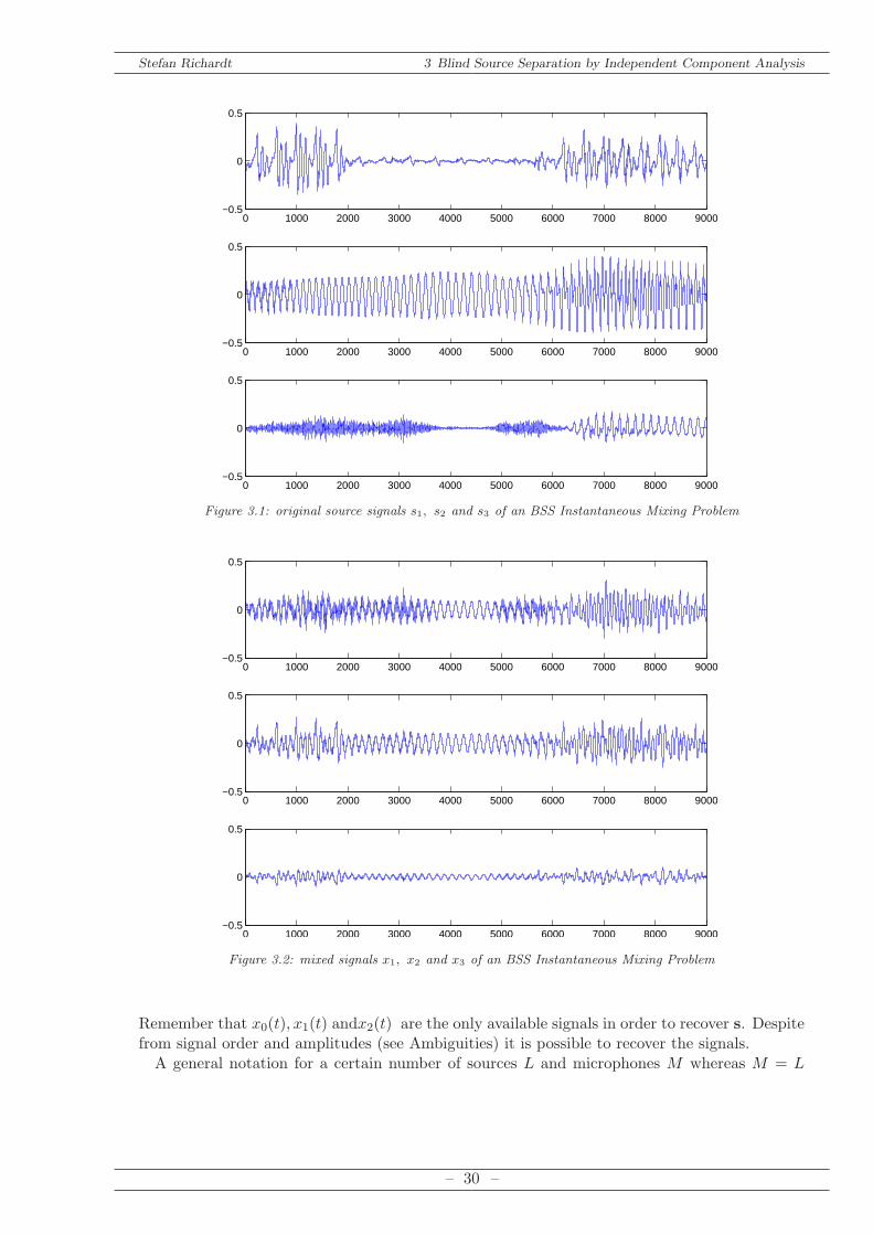
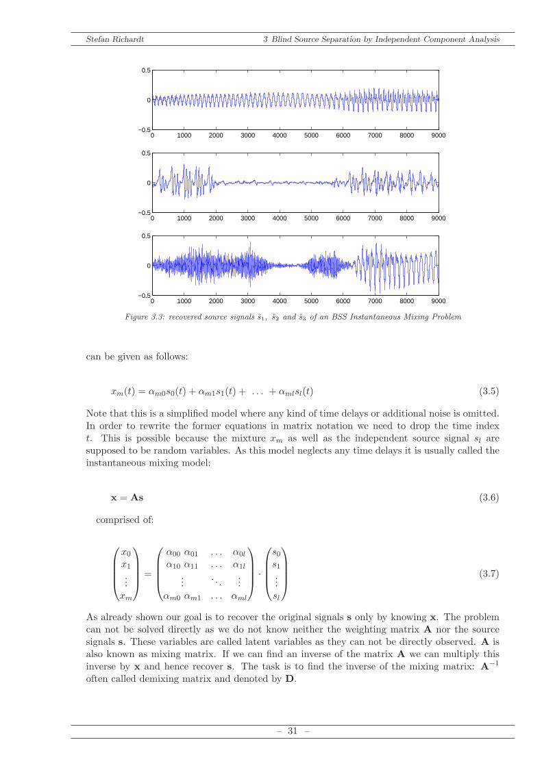
As example the mixing and demixing process is shown in the following figures. The independentsource signals s0(t), s1(t) and s2(t) in Figure 3.1 are multiplied by the unknown mixing matrixA which leads to the observed signals x0(t), x1(t) and x2(t) in Figure 3.2. The estimated signalss0(t), s.1(t) and s2(t) are depicted in Figure 3.3.
– 29 –
Stefan Richardt 3 Blind Source Separation by Independent Component Analysis
0 1000 2000 3000 4000 5000 6000 7000 8000 9000−0.5
0
0.5
0 1000 2000 3000 4000 5000 6000 7000 8000 9000−0.5
0
0.5
0 1000 2000 3000 4000 5000 6000 7000 8000 9000−0.5
0
0.5
Figure 3.1: original source signals s1, s2 and s3 of an BSS Instantaneous Mixing Problem
0 1000 2000 3000 4000 5000 6000 7000 8000 9000−0.5
0
0.5
0 1000 2000 3000 4000 5000 6000 7000 8000 9000−0.5
0
0.5
0 1000 2000 3000 4000 5000 6000 7000 8000 9000−0.5
0
0.5
Figure 3.2: mixed signals x1, x2 and x3 of an BSS Instantaneous Mixing Problem
Remember that x0(t), x1(t) andx2(t) are the only available signals in order to recover s. Despitefrom signal order and amplitudes (see Ambiguities) it is possible to recover the signals.A general notation for a certain number of sources L and microphones M whereas M = L
– 30 –
Stefan Richardt 3 Blind Source Separation by Independent Component Analysis
0 1000 2000 3000 4000 5000 6000 7000 8000 9000−0.5
0
0.5
0 1000 2000 3000 4000 5000 6000 7000 8000 9000−0.5
0
0.5
0 1000 2000 3000 4000 5000 6000 7000 8000 9000−0.5
0
0.5
Figure 3.3: recovered source signals s1, s2 and s3 of an BSS Instantaneous Mixing Problem
can be given as follows:
xm(t) = αm0s0(t) + αm1s1(t) + . . . + αmlsl(t) (3.5)
Note that this is a simplified model where any kind of time delays or additional noise is omitted.In order to rewrite the former equations in matrix notation we need to drop the time indext. This is possible because the mixture xm as well as the independent source signal sl aresupposed to be random variables. As this model neglects any time delays it is usually called theinstantaneous mixing model:
x = As (3.6)
comprised of:
x0x1...
xm
=
α00 α01 . . . α0l
α10 α11 . . . α1l
.... . .
...αm0 αm1 . . . αml
·
s0s1...sl
(3.7)
As already shown our goal is to recover the original signals s only by knowing x. The problemcan not be solved directly as we do not know neither the weighting matrix A nor the sourcesignals s. These variables are called latent variables as they can not be directly observed. A isalso known as mixing matrix. If we can find an inverse of the matrix A we can multiply thisinverse by x and hence recover s. The task is to find the inverse of the mixing matrix: A−1
often called demixing matrix and denoted by D.
– 31 –
Stefan Richardt 3 Blind Source Separation by Independent Component Analysis
D
ŝ0
ŝL-1
A
x0
xL-1
s0
sL-1
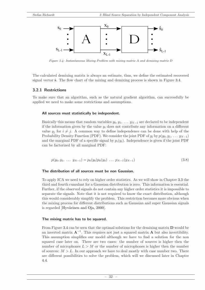
Figure 3.4: Instantaneous Mixing Problem with mixing matrix A and demixing matrix D
The calculated demixing matrix is always an estimate, thus, we define the estimated recoveredsignal vector s. The flow chart of the mixing and demixing process is shown in Figure 3.4.
3.2.1 Restrictions
To make sure that an algorithm, such as the natural gradient algorithm, can successfully beapplied we need to make some restrictions and assumptions.
All sources must statistically be independent.
Basically this means that random variables y0, y1, . . . yN−1 are declared to be independentif the information given by the value yi does not contribute any information on a differentvalue yj for i 6= j. A common way to define independence can be done with help of theProbability Density Function (PDF). We consider the joint PDF of yi by p(y0, y1, . . . yN−1)and the marginal PDF of a specific signal by pi(yi). Independence is given if the joint PDFcan be factorized by all marginal PDF:
p(y0, y1, . . . yN−1) = p0(y0)p0(y0) . . . pN−1(yN−1) (3.8)
The distribution of all sources must be non Gaussian.
To apply ICA we need to rely on higher order statistics. As we will show in Chapter 3.3 thethird and fourth cumulant for a Gaussian distribution is zero. This information is essential.Further, if the observed signals do not contain any higher order statistics it is impossible toseparate the signals. Note that it is not required to know the exact distribution, althoughthis would considerably simplify the problem. This restriction becomes more obvious whenthe mixing process for different distributions such as Gaussian and super Gaussian signalsis regarded [Hyvarinen and Oja, 2000].
The mixing matrix has to be squared.
From Figure 3.4 can be seen that the optimal solutions for the demixing matrixD would bean inverted matrix A−1. This requires not just a squared matrix A but also invertibility.This assumption simplifies our model although we have to find a solution for the nonsquared case later on. There are two cases: the number of sources is higher then thenumber of microphones L > M or the number of microphones is higher then the numberof sources: M > L. In our approach we have to deal mostly with case number two. Thereare different possibilities to solve the problem, which will we discussed later in Chapter4.4.
– 32 –
Stefan Richardt 3 Blind Source Separation by Independent Component Analysis
3.2.2 Ambiguities
There are two ambiguities of ICA. It is important to consider them when implementing thealgorithm as this will affect but also restrict the algorithm.
The signal energy can not be determined.
The problem is that neither A nor s is known. Introducing an additional random scalarγl we scale the source vector s while dividing every column of A by the corresponding γl.Although the variance of s is changed the same result is provided. Based on Equation(3.6) the problem can be noted as follows:
x = As (3.9)
introducing the scalar γl:
x0x1...
xm
=
1γ0α00
1γ1α01 . . . 1
γlα0l
1γ0α10
1γ1α11 . . . 1
γlα1l
.... . .
...1γ0αm0
1γ1αm1 . . . 1
γlαml
·
γ0 s0γ1 s1...
γl sl
(3.10)
Hence, there is a need in constraining the signal energy in our approach. For example,this can be done by a simple normalization of the recovered signals.
The order of the independent components can not be determined.
Again, we are facing the problem that neither A nor s is known. It is possible to freelychange the order of the independent sources. Any of the sources can considered to be first.We can easily change the order of sources s without affecting x. As an example, referringagain to Equation (3.6), we interchange s0 and s1 while shifting the corresponding columnsof A:
x0x1...
xm
=
α01 α00 . . . α0l
α11 α10 . . . α1l
.... . .
...αm1 αm0 . . . αml
·
s1s0...sl
(3.11)
Having explained the basic idea of BSS respectively ICA with all its assumptions and ambiguitieswe need to find an algorithm in order to estimate the demixing matrix D referring to figure 3.4.The algorithm should work reliably and fast. At this point we want to introduce the naturalgradient algorithm.
– 33 –
Stefan Richardt 3 Blind Source Separation by Independent Component Analysis
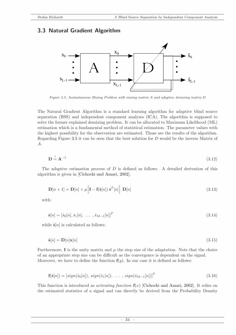
3.3 Natural Gradient Algorithm
ŝ0
ŝL-1
A
x0
xL-1
s0
sL-1
Figure 3.5: Instantaneous Mixing Problem with mixing matrix A and adaptive demixing matrix D
The Natural Gradient Algorithm is a standard learning algorithm for adaptive blind sourceseparation (BSS) and independent component analyses (ICA). The algorithm is supposed tosolve the former explained demixing problem. It can be allocated to Maximum Likelihood (ML)estimation which is a fundamental method of statistical estimation. The parameter values withthe highest possibility for the observation are estimated. Those are the results of the algorithm.Regarding Figure 3.5 it can be seen that the best solution for D would be the inverse Matrix ofA.
D!= A−1 (3.12)
The adaptive estimation process of D is defined as follows. A detailed derivation of thisalgorithm is given in [Cichocki and Amari, 2002].
D[n+ 1] = D[n] + µ[
I− f(s[n]) sT [n]]
D[n] (3.13)
with:
s[n] = [s0[n], s1[n], . . . , sM−1[n]]T (3.14)
while s[n] is calculated as follows:
s[n] = D[n]x[n] (3.15)
Furthermore, I is the unity matrix and µ the step size of the adaptation. Note that the choiceof an appropriate step size can be difficult as the convergence is dependent on the signal.Moreover, we have to define the function f(y). In our case it is defined as follows:
f(s[n]) = [sign(s0[n]), sign(s1[n]), . . . , sign(sM−1[n])]T (3.16)
This function is introduced as activating function f(x) [Cichocki and Amari, 2002]. It relies onthe estimated statistics of a signal and can directly be derived from the Probability Density
– 34 –
Stefan Richardt 3 Blind Source Separation by Independent Component Analysis
Function (PDF), q(x).
f(x) = −d log q(x)
dx(3.17)
Knowing or estimating the PDF of a signal, the activating function can be derived and appliedto the Natural Gradient Algorithm. Therefore, in order to implement the Natural GradientAlgorithm we need to know the statistics of the expected signals. A different PDF leads to adifferent activating function. Hence, two well known examples are given: The PDF q(x) andthe corresponding, activating function f(x) of a Gaussian and a Laplace distribution.
Gauss: q(x) =1√2πσ2
e−(x− µ)2
2σ2⇒ f(x) =
x
σ2(3.18)
Laplace: q(x) =1
2σe−
|x− µ|σ
⇒ f(x) =sign(x)
σ(3.19)
For other distributions and its corresponding activating functions see [Cichocki and Amari,2002]. Note that zero-mean signals with µ = 0 are assumed and for simplicity the variance isset by σ2 = 1.It is common to classify signals due to their statistical properties. Statistical moments like the
mean value µ or the variance σ2 describe the distribution of a signal. From Equation 3.18 can beseen that the normal or Gaussian distribution can fully be described by these two parameters.Another distribution, fitting the features of speech best, is the Laplace distribution. At this pointwe want to introduce the third moment and fourth satistical moment which are: skewness γ andkurtosis γ2. Although the third moment is zero the fourth moment of the Laplace distribution isknown to be γ2 = 3. It is not needed to define the distribution, however, it is inherent. Accordingto [Hyvarinen and Oja, 2000], where a detailed explanation is given, higher order statistics arenecessary if a successful BSS using ICA shall be applied. This leads to a nonlinear activatingfunction as shown in Equation 3.19. A good overview of stochastic signals and estimations isgiven in [Vary and Martin, 2006].The Laplace distribution is known to match the statistical properties of speech best. Conse-
quently, the corresponding activation function f(x) is implemented. It is obvious that if anotherdistribution is expected its corresponding function needs to be implemented.
– 35 –
Stefan Richardt 4 Blind Source Separation by Frequency Invariant Beamforming
4 Blind Source Separation by Frequency
Invariant Beamforming
The applied approach, suggested in [Liu and Mandic, 2005] and [Liu, 2010], combines the formerexplained techniques. The algorithm contains two successive stages:
Frequency Invariant Beamforming Network
Blind Source Separation Algorithm
A beamforming network, consisting of several FIB, scans the room while the BSS algorithmis supposed to estimate a set of coefficients whereby the beamformers are weighted. The rela-tionship of the beamformers coefficients determines from which DOA angle signals are eitherenhanced or suppressed.
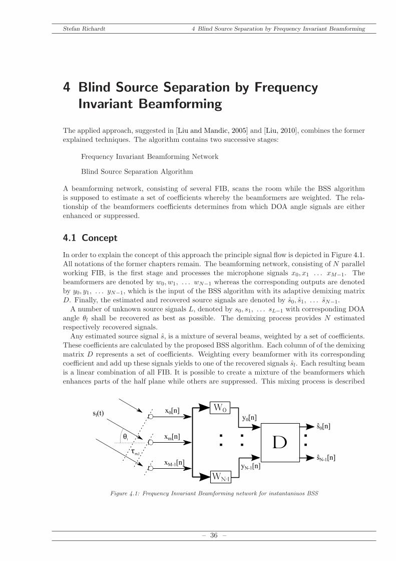
4.1 Concept
In order to explain the concept of this approach the principle signal flow is depicted in Figure 4.1.All notations of the former chapters remain. The beamforming network, consisting of N parallelworking FIB, is the first stage and processes the microphone signals x0, x1 . . . xM−1. Thebeamformers are denoted by w0, w1, . . . wN−1 whereas the corresponding outputs are denotedby y0, y1, . . . yN−1, which is the input of the BSS algorithm with its adaptive demixing matrixD. Finally, the estimated and recovered source signals are denoted by s0, s1, . . . sN−1.A number of unknown source signals L, denoted by s0, s1, . . . sL−1 with corresponding DOA
angle θl shall be recovered as best as possible. The demixing process provides N estimatedrespectively recovered signals.Any estimated source signal s, is a mixture of several beams, weighted by a set of coefficients.
These coefficients are calculated by the proposed BSS algorithm. Each column of of the demixingmatrix D represents a set of coefficients. Weighting every beamformer with its correspondingcoefficient and add up these signals yields to one of the recovered signals sl. Each resulting beamis a linear combination of all FIB. It is possible to create a mixture of the beamformers whichenhances parts of the half plane while others are suppressed. This mixing process is described
sl(t)x0[n]
xm[n]
xM-1[n]
w0
wN-1
D
ŝ0[n]
ŝN-1[n]
θl
τm,l
y0[n]
yN-1[n]
Figure 4.1: Frequency Invariant Beamforming network for instantaniuos BSS
– 36 –
Stefan Richardt 4 Blind Source Separation by Frequency Invariant Beamforming
and depicted in Chapter 4.3. The optimization process of the adaptive coefficients is performedby the BSS algorithm, described in Chapter 3. Note that the input signals in this case arealready the outputs of the beamformers.As we most likely have more then one source we want to recover all source signals. Hence,
we determine several mixes in parallel, which are supposed to recover the inputs from differentDOA angles as best as possible. The BSS algorithm is creating several mixes of the beamformersoutputs. According to Equation (3.1) the demixing Matrix D has to be squared and with anumber of beamformers N = 7 the same number of recovered signals is received accordingly,even if we expect or know that the number of speakers is lower. Hence, we have to reducethe number of recovered signals or simply spot the right results. The method of singular valuedecomposition reduces the number of signals before the BSS algorithm is applied and is explainedin chapter 4.4. Another possibility would be a modified BSS algorithm addressing the problem ofan overdetermined model, which is proposed in [Zhang et al., 1999] but has not been implementedyet.
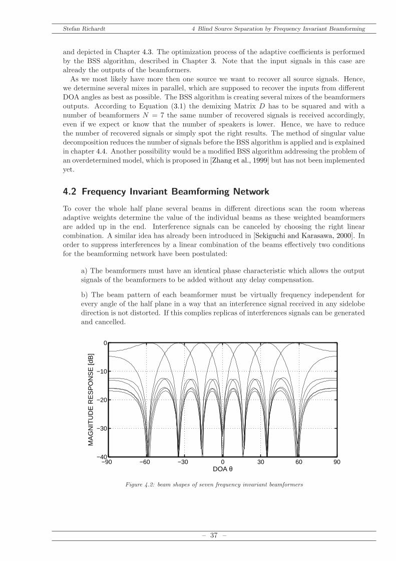
4.2 Frequency Invariant Beamforming Network
To cover the whole half plane several beams in different directions scan the room whereasadaptive weights determine the value of the individual beams as these weighted beamformersare added up in the end. Interference signals can be canceled by choosing the right linearcombination. A similar idea has already been introduced in [Sekiguchi and Karasawa, 2000]. Inorder to suppress interferences by a linear combination of the beams effectively two conditionsfor the beamforming network have been postulated:
a) The beamformers must have an identical phase characteristic which allows the outputsignals of the beamformers to be added without any delay compensation.
b) The beam pattern of each beamformer must be virtually frequency independent forevery angle of the half plane in a way that an interference signal received in any sidelobedirection is not distorted. If this complies replicas of interferences signals can be generatedand cancelled.
−90 −60 −30 0 30 60 90−40
−30
−20
−10
0
DOA θ
MA
GN
ITU
DE
RE
SP
ON
SE
[dB
]
Figure 4.2: beam shapes of seven frequency invariant beamformers
– 37 –
Stefan Richardt 4 Blind Source Separation by Frequency Invariant Beamforming
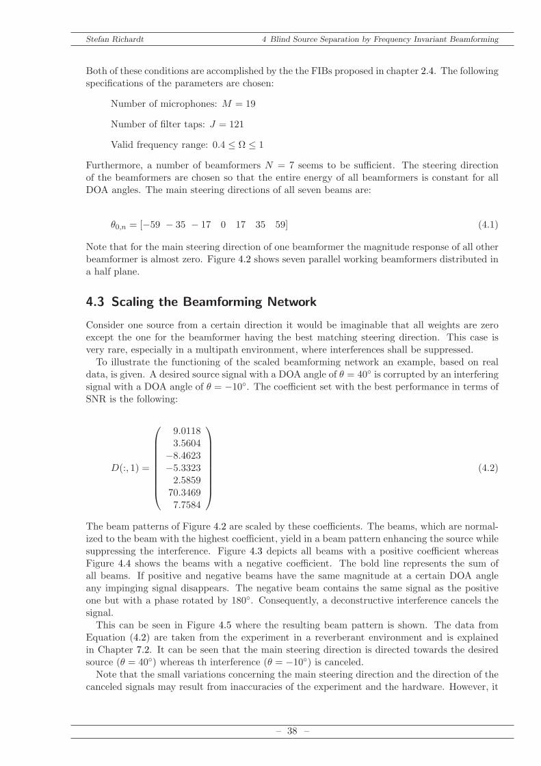
Both of these conditions are accomplished by the the FIBs proposed in chapter 2.4. The followingspecifications of the parameters are chosen:
Number of microphones: M = 19
Number of filter taps: J = 121
Valid frequency range: 0.4 ≤ Ω ≤ 1
Furthermore, a number of beamformers N = 7 seems to be sufficient. The steering directionof the beamformers are chosen so that the entire energy of all beamformers is constant for allDOA angles. The main steering directions of all seven beams are:
θ0,n = [−59 − 35 − 17 0 17 35 59] (4.1)
Note that for the main steering direction of one beamformer the magnitude response of all otherbeamformer is almost zero. Figure 4.2 shows seven parallel working beamformers distributed ina half plane.
4.3 Scaling the Beamforming Network
Consider one source from a certain direction it would be imaginable that all weights are zeroexcept the one for the beamformer having the best matching steering direction. This case isvery rare, especially in a multipath environment, where interferences shall be suppressed.To illustrate the functioning of the scaled beamforming network an example, based on real
data, is given. A desired source signal with a DOA angle of θ = 40 is corrupted by an interferingsignal with a DOA angle of θ = −10. The coefficient set with the best performance in terms ofSNR is the following:
D(:, 1) =
9.01183.5604
−8.4623−5.33232.585970.34697.7584
(4.2)
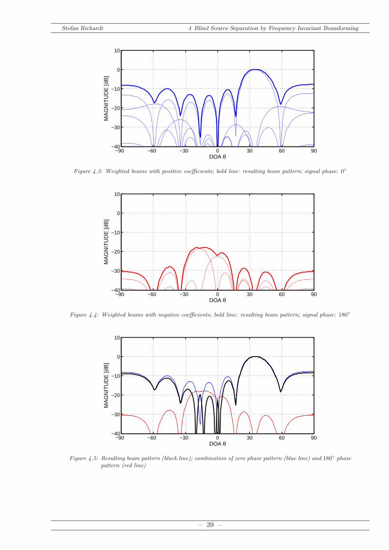
The beam patterns of Figure 4.2 are scaled by these coefficients. The beams, which are normal-ized to the beam with the highest coefficient, yield in a beam pattern enhancing the source whilesuppressing the interference. Figure 4.3 depicts all beams with a positive coefficient whereasFigure 4.4 shows the beams with a negative coefficient. The bold line represents the sum ofall beams. If positive and negative beams have the same magnitude at a certain DOA angleany impinging signal disappears. The negative beam contains the same signal as the positiveone but with a phase rotated by 180. Consequently, a deconstructive interference cancels thesignal.This can be seen in Figure 4.5 where the resulting beam pattern is shown. The data from
Equation (4.2) are taken from the experiment in a reverberant environment and is explainedin Chapter 7.2. It can be seen that the main steering direction is directed towards the desiredsource (θ = 40) whereas th interference (θ = −10) is canceled.Note that the small variations concerning the main steering direction and the direction of the
canceled signals may result from inaccuracies of the experiment and the hardware. However, it
– 38 –
Stefan Richardt 4 Blind Source Separation by Frequency Invariant Beamforming
−90 −60 −30 0 30 60 90−40
−30
−20
−10
0
10
DOA θ
MA
GN
ITU
DE
[dB
]
Figure 4.3: Weighted beams with positive coefficients; bold line: resulting beam pattern; signal phase: 0
−90 −60 −30 0 30 60 90−40
−30
−20
−10
0
10
DOA θ
MA
GN
ITU
DE
[dB
]
Figure 4.4: Weighted beams with negative coefficients; bold line: resulting beam pattern; signal phase: 180
−90 −60 −30 0 30 60 90−40
−30
−20
−10
0
10
DOA θ
MA
GN
ITU
DE
[dB
]
Figure 4.5: Resulting beam pattern (black line); combination of zero phase pattern (blue line) and 180 phasepattern (red line)
– 39 –
Stefan Richardt 4 Blind Source Separation by Frequency Invariant Beamforming
is shown that the final beamformer is working properly. Even if the interference source matchesnot exactly the minimum of the resulting beam the interference is at least attenuated by 20 dB.Figure 4.5 shows that more than one minimum exists. Hence, the algorithm is capable to cancelmultiple interferences. It is conceivable that a major interference is a specific reflection of aninterfering source whereas the beamformer is capable to cancel this reflection.
4.4 Singular Value Decomposition
As Singular Value Decomposition is utilized in order to reduce the number of resulting signalsa short introduction to the topic is given. Furthermore, it is explained how this method can beintegrated in the proposed algorithm.Singular Value Decomposition (SVD) is a method to factorize a non squared matrix. It is
closely related to Eigen Value Decomposition (EVD), also known as eigendecomposition, whereasthis mathematical problem requires a squared matrix.A general mathematical description of eigendecomposition can be given by:
A = QΛQH (4.3)
A squared Matrix A with dimensions [N × N ] and N linear independent eigenvectors qi withi ∈ [1, 2, . . . , N ] can be factorized by the eigen vector matrix Q. It contains the eigen vectorsqi in the i-th column whereas the diagonal matrix Λ contains the corresponding eigenvalues λi.Hence, A is represented by its eigen values and its eigen vectors. In Matlab the function eig isavailable in order to execute a EVD.Singular value decomposition is closely related to eigendecomposition. A non squared matrix
Y with dimensions [N × S] can be factorized as follows:
Y = UΛV H (4.4)
Similar to the eigen vector matrix Q the columns of U are the eigenvectors of Y Y H and arecalled left singular vectors. The columns of V are the eigenvectors of Y HY and named rightsingular vectors. The non zero elements of Λ, labeled as non zero singular values, are the squareroots of the non zero eigenvalues of either Y HY or Y Y H . The corresponding Matlab function,which is also utilized in course of this work is called svd.SVD in our case is applied to reduce the number of recovered signals. In order to make use
of the BSS algorithm, which provides the same number of outputs as inputs, the number ofinput signals has to be reduced before applying the BSS algorithm. We assume that the numberof sources is known and described by L. It is supposed that the number of beamformers N ishigher then the number of sources:
N > L (4.5)
Additionally, we need to define S as the number of samples. The goal of the applied SVD isto reduce the number of output vectors of the beamforming network to L. We suppose thatthe outputs of the beamformer, described by the matrix Y , only contain L linear independentsignals. Hence, the rank of the matrix Y equals L, this means that only L eigenvalues withλ 6= 0 exist. The problem can be explained best by regarding the matrices and the according
– 40 –
Stefan Richardt 4 Blind Source Separation by Frequency Invariant Beamforming
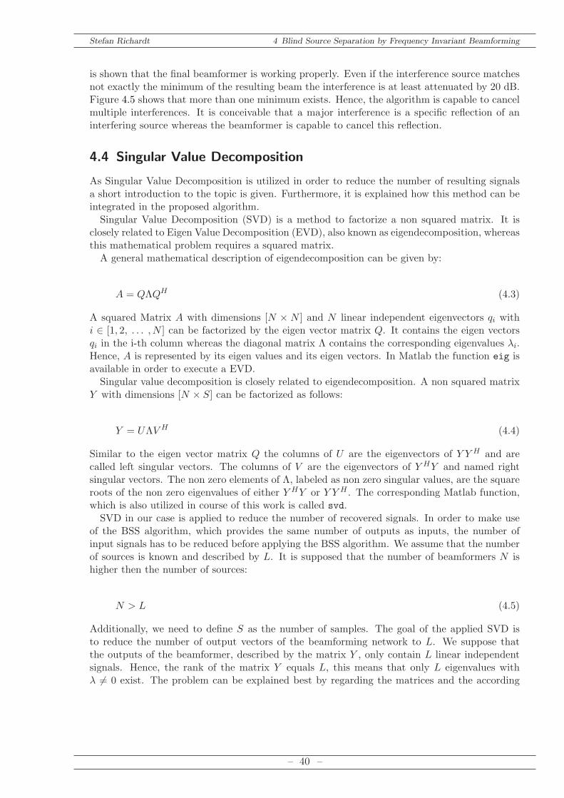
dimensions from Equation (4.4):
Y︸︷︷︸
[N×S]
= U︸︷︷︸
[N×N ]
· Λ︸︷︷︸
[N×S]
· V H︸︷︷︸
[S×S]
(4.6)
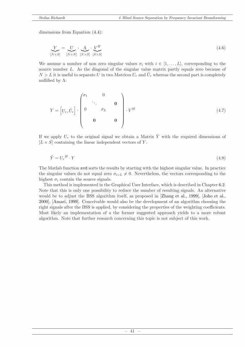
We assume a number of non zero singular values σi with i ∈ [1, . . . , L], corresponding to thesource number L. As the diagonal of the singular value matrix partly equals zero because ofN > L it is useful to separate U in two Matrices Ur and Ur whereas the second part is completelynullified by Λ:
Y =[
Ur, Ur
]
·
σ1 0
. . . 0
0 σL
0 0
· V H (4.7)
If we apply Ur to the original signal we obtain a Matrix Y with the required dimensions of[L× S] containing the linear independent vectors of Y .
Y = UrH · Y (4.8)
The Matlab function svd sorts the results by starting with the highest singular value. In practicethe singular values do not equal zero σi>L 6= 0. Nevertheless, the vectors corresponding to thehighest σi contain the source signals.This method is implemented in the Graphical User Interface, which is described in Chapter 6.2.
Note that this is only one possibility to reduce the number of resulting signals. An alternativewould be to adjust the BSS algorithm itself, as proposed in [Zhang et al., 1999], [Joho et al.,2000], [Amari, 1999]. Conceivable would also be the development of an algorithm choosing theright signals after the BSS is applied, by considering the properties of the weighting coefficients.Most likely an implementation of a the former suggested approach yields to a more robustalgorithm. Note that further research concerning this topic is not subject of this work.
– 41 –

Stefan Richardt 4 Blind Source Separation by Frequency Invariant Beamforming
Part II
Practical Approach
– 42 –
Stefan Richardt 5 Hardware
5 Hardware
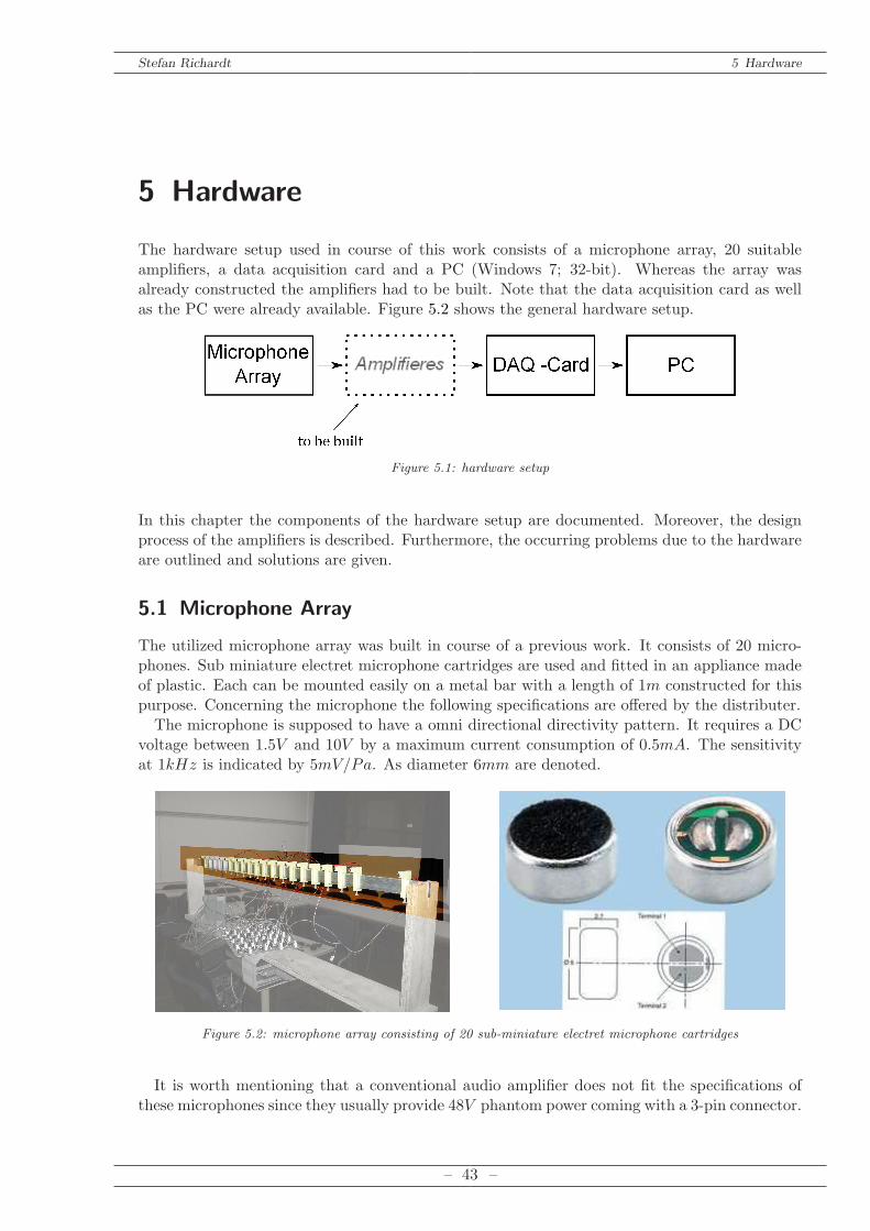
The hardware setup used in course of this work consists of a microphone array, 20 suitableamplifiers, a data acquisition card and a PC (Windows 7; 32-bit). Whereas the array wasalready constructed the amplifiers had to be built. Note that the data acquisition card as wellas the PC were already available. Figure 5.2 shows the general hardware setup.
Microphone
Array
Figure 5.1: hardware setup
In this chapter the components of the hardware setup are documented. Moreover, the designprocess of the amplifiers is described. Furthermore, the occurring problems due to the hardwareare outlined and solutions are given.
5.1 Microphone Array
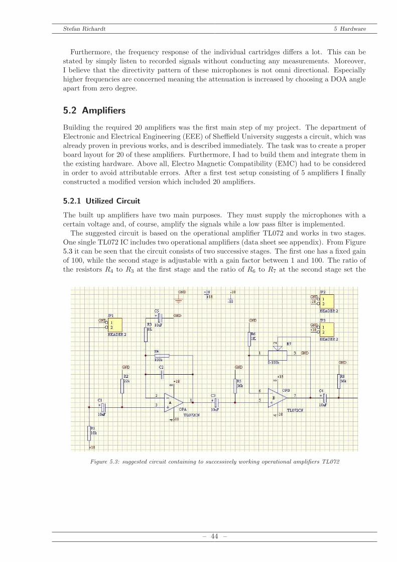
The utilized microphone array was built in course of a previous work. It consists of 20 micro-phones. Sub miniature electret microphone cartridges are used and fitted in an appliance madeof plastic. Each can be mounted easily on a metal bar with a length of 1m constructed for thispurpose. Concerning the microphone the following specifications are offered by the distributer.The microphone is supposed to have a omni directional directivity pattern. It requires a DC
voltage between 1.5V and 10V by a maximum current consumption of 0.5mA. The sensitivityat 1kHz is indicated by 5mV/Pa. As diameter 6mm are denoted.
Figure 5.2: microphone array consisting of 20 sub-miniature electret microphone cartridges
It is worth mentioning that a conventional audio amplifier does not fit the specifications ofthese microphones since they usually provide 48V phantom power coming with a 3-pin connector.
– 43 –
Stefan Richardt 5 Hardware
Furthermore, the frequency response of the individual cartridges differs a lot. This can bestated by simply listen to recorded signals without conducting any measurements. Moreover,I believe that the directivity pattern of these microphones is not omni directional. Especiallyhigher frequencies are concerned meaning the attenuation is increased by choosing a DOA angleapart from zero degree.
5.2 Amplifiers
Building the required 20 amplifiers was the first main step of my project. The department ofElectronic and Electrical Engineering (EEE) of Sheffield University suggests a circuit, which wasalready proven in previous works, and is described immediately. The task was to create a properboard layout for 20 of these amplifiers. Furthermore, I had to build them and integrate them inthe existing hardware. Above all, Electro Magnetic Compatibility (EMC) had to be consideredin order to avoid attributable errors. After a first test setup consisting of 5 amplifiers I finallyconstructed a modified version which included 20 amplifiers.
5.2.1 Utilized Circuit
The built up amplifiers have two main purposes. They must supply the microphones with acertain voltage and, of course, amplify the signals while a low pass filter is implemented.The suggested circuit is based on the operational amplifier TL072 and works in two stages.
One single TL072 IC includes two operational amplifiers (data sheet see appendix). From Figure5.3 it can be seen that the circuit consists of two successive stages. The first one has a fixed gainof 100, while the second stage is adjustable with a gain factor between 1 and 100. The ratio ofthe resistors R4 to R3 at the first stage and the ratio of R6 to R7 at the second stage set the
Figure 5.3: suggested circuit containing to successively working operational amplifiers TL072
– 44 –
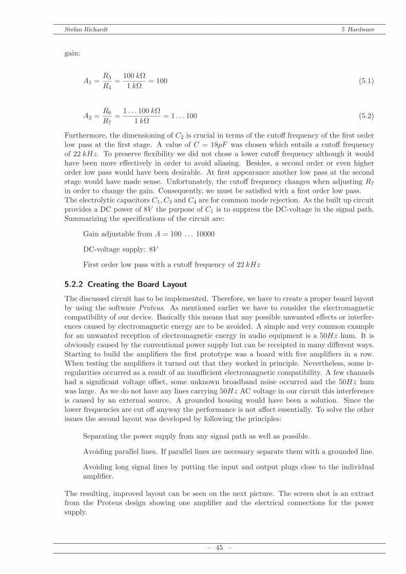
Stefan Richardt 5 Hardware
gain:
A1 =R3
R4=
100 kΩ
1 kΩ= 100 (5.1)
A2 =R6
R7=
1 . . . 100 kΩ
1 kΩ= 1 . . . 100 (5.2)
Furthermore, the dimensioning of C2 is crucial in terms of the cutoff frequency of the first orderlow pass at the first stage. A value of C = 18pF was chosen which entails a cutoff frequencyof 22 kHz. To preserve flexibility we did not chose a lower cutoff frequency although it wouldhave been more effectively in order to avoid aliasing. Besides, a second order or even higherorder low pass would have been desirable. At first appearance another low pass at the secondstage would have made sense. Unfortunately, the cutoff frequency changes when adjusting R7
in order to change the gain. Consequently, we must be satisfied with a first order low pass.The electrolytic capacitors C1, C3 and C4 are for common mode rejection. As the built up circuitprovides a DC power of 8V the purpose of C1 is to suppress the DC-voltage in the signal path.Summarizing the specifications of the circuit are:
Gain adjustable from A = 100 . . . 10000
DC-voltage supply: 8V
First order low pass with a cutoff frequency of 22 kHz
5.2.2 Creating the Board Layout
The discussed circuit has to be implemented. Therefore, we have to create a proper board layoutby using the software Proteus. As mentioned earlier we have to consider the electromagneticcompatibility of our device. Basically this means that any possible unwanted effects or interfer-ences caused by electromagnetic energy are to be avoided. A simple and very common examplefor an unwanted reception of electromagnetic energy in audio equipment is a 50Hz hum. It isobviously caused by the conventional power supply but can be receipted in many different ways.Starting to build the amplifiers the first prototype was a board with five amplifiers in a row.When testing the amplifiers it turned out that they worked in principle. Nevertheless, some ir-regularities occurred as a result of an insufficient electromagnetic compatibility. A few channelshad a significant voltage offset, some unknown broadband noise occurred and the 50Hz humwas large. As we do not have any lines carrying 50Hz AC voltage in our circuit this interferenceis caused by an external source. A grounded housing would have been a solution. Since thelower frequencies are cut off anyway the performance is not affect essentially. To solve the otherissues the second layout was developed by following the principles:
Separating the power supply from any signal path as well as possible.
Avoiding parallel lines. If parallel lines are necessary separate them with a grounded line.
Avoiding long signal lines by putting the input and output plugs close to the individualamplifier.
The resulting, improved layout can be seen on the next picture. The screen shot is an extractfrom the Proteus design showing one amplifier and the electrical connections for the powersupply.
– 45 –
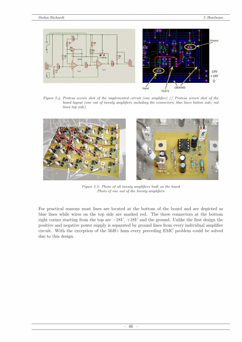
Stefan Richardt 5 Hardware
-18V
+18V
GROUNDInput
Output
TL072
Figure 5.4: Proteus screen shot of the implemented circuit (one amplifier) // Proteus screen shot of theboard layout (one out of twenty amplifiers including the connectors; blue lines button side; redlines top side)
Figure 5.5: Photo of all twenty amplifiers built on the boardPhoto of one out of the twenty amplifiers
For practical reasons most lines are located at the bottom of the board and are depicted asblue lines while wires on the top side are marked red. The three connectors at the bottomright corner starting from the top are −18V , +18V and the ground. Unlike the first design thepositive and negative power supply is separated by ground lines from every individual amplifiercircuit. With the exception of the 50Hz hum every preceding EMC problem could be solveddue to this design.
– 46 –
Stefan Richardt 5 Hardware
5.3 DAQ - card
5.3.1 Specifications
The utilized data acquisition card Adlink DAQ-2205 is the main interface of our system. Itlinks the analogue equipment directly with the PC via PCI bus. In interaction with the Matlabdata acquisition toolbox a direct data access with Matlab is possible. The data acquisition cardsupports 64 single ended analog input channels or 32 differential analog input channels. As theoccurring signals share a common ground the maximal possible utilization of the card are 64channels in theory. The A-D converter operates with a resolution of 16 bit with an input rangeof +/- 10 V . Furthermore, the card allocates programmable gains of x1, x2, x4 and x8, whichallows the user to adapt the systems in terms of signal range by software. The card also providestwo analogue outputs with 12-bit resolution and several digital in - and outputs.Utilizing Adlink DAQ-2205 a certain number of problems occurred, which are discussed in the
following sections. The manufacturer claims a 500 kSs acquisition. The sampling rate has to be
divided by the number of used channels as a multiplexer for AD conversion is used. Due to themultiplexer two major problems result. Firstly, we face a limited sample rate, thus, the problemof a proper anti aliasing filter occurs. Secondly, we have to deal with a non-simultaneously dataacquisition. Furthermore, coupling appears mainly caused by the breakout cable which connectsthe DAQ card and the amplifiers.
5.3.2 Limited Sample Rate and Aliasing
The first issue we have to deal with is a decreasing sampling rate when increasing the numberof channels. Using all of the 64 channels yields to a theoretical sampling rate of:
fs =f
Mchan=
500000Hz
64≈ 7800Hz (5.3)
Considering the Nyquist theorem we obtain the following maximum frequency:
fmax =fs2
= 3900Hz (5.4)
To effectively achieve the calculated frequency an ideal, analogue, rectangular anti aliasing filterwould be required. However, even higher order analogue filters do not fully accomplish theserequirements consequently the maximum frequency decreases again. In our case the built upamplifiers provide just a first order low pass so that oversampling is absolutely nessecairy whenadditional higher order filters are not used. Our specific approach with 19 channels leads to atheoretical sampling rate of:
fs =f
Mchan=
500000Hz
19≈ 26316Hz (5.5)
In practice the sample rate is determined by fs = 24999Hz. A good explanation how to avoidaliasing by utilizing oversampling and a simple analogue filter is given in [Oppenheim et al.,2004]. Our approach is quite similar. We use oversampling to simplify an anti aliasing filterwhile making it more cost effective via a software implementation. A simple low pass filteris provided by the amplifiers. Note the the cutoff frequency actually is too high. Due to thefact that the signal energy at higher frequencies (f > 12.5 kHz) is low enough aliasing of thesefrequencies does not affect the results significantly. According to the signal specification we now
– 47 –
Stefan Richardt 5 Hardware
apply the A-D conversion in a way that we are not affected by any aliased signals or noise. Thesample rate of the converter is high enough to ensure that no significant signal components overfs/2, which would cause aliasing, occur. In our case this is accomplished when using a samplingrate of 24999Hz.Under these conditions we can easily apply a sharp digital low pass. The cutoff frequency in
our case is 4150Hz and, therefore, matched with our sampling rate reduction of F = 3. As aresult fs = 8333Hz and, consequently, fmax = 4161Hz.As mentioned earlier, dealing with speech signals a maximum frequency of at least 4000Hz
is desirable. The reason for that is that the majority of the information is situated in frequencyranges below 4000 Hz. Besides, we can assume that signals with frequencies over 12500 Hz,which equals fs/2 are not crucial simply because of their low magnitudes. In our case this isreally important whereas it is not possible to avoid aliasing in this frequency range due to thelack of a appropriate analogue filters.Regarding the current setup leads to the conclusion that its maximum of channels is reached.
If it is necessary to increase the number of channels, higher order analogue low pass filters wouldbe required. Increasing the number of channels without adding additional analogue filters wouldentail either a reduction of the sampling rate or a significant deterioration of the anti aliasingfilter. This in turn, would lead to clearly perceptible distortions in the recordings.
5.3.3 Non Simultaneously Acquisition
The second issue is the successive A-D conversion of every single channel. Unfortunately, thecard does not include any on board sample and hold devices. To ensure simultaneous dataacquisition sample and hold devices are necessary when using a multiplexer. Usually theyare already part of a multichannel A-D converter. The impact caused by not reading in thechannels simultaneously can easily be compared with a shift of the angle of the incoming signal.Considering a signal with an impinging angle of zero degree we should obtain the same signal atevery microphone if the above mentioned conditions are complied. If the processing of the A-Dconversion is successive every channel is delayed by a multiple of the time delay TAD. This leadsto a constant shift of the steering direction of the hole system. According to the manufacturerthe additional time delay between two sampled channels can be calculated as followed:
TAD =counter sampling interval
timebase=
80
40MHz= 2µs (5.6)
which equals:
TAD =1
fs=
1
500000Hz= 2µs (5.7)
To circumvent the problem Adlink provides a signal for external sample and hold devices. Soit would be possible to insert a sample and hold device for each of the channels between theamplifiers output and the signal input of the card. The card itself would provide a control signalfor every of these devices. As a result the analog inputs would be sampled at the same time.Making use of this feature the problems could be solved in hardware. Compared with a
software solution no additional latency is caused while saving performance of the PC whichcould be a crucial point in terms of a real time implementation. Nevertheless, it would be quitea big effort to build and include all the hardware.Another solution is to compensate the delay via software. This solution requires one FIR filter
per channel to apply the appropriate delay. For further information concerning fractional delayplease refer to Chapter 2.4.5.
– 48 –
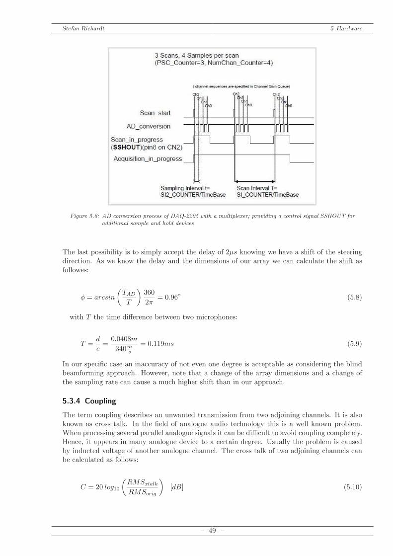
Stefan Richardt 5 Hardware
Figure 5.6: AD conversion process of DAQ-2205 with a multiplexer; providing a control signal SSHOUT foradditional sample and hold devices
The last possibility is to simply accept the delay of 2µs knowing we have a shift of the steeringdirection. As we know the delay and the dimensions of our array we can calculate the shift asfollowes:
φ = arcsin
(TAD
T
)360
2π= 0.96 (5.8)
with T the time difference between two microphones:
T =d
c=
0.0408m
340ms
= 0.119ms (5.9)
In our specific case an inaccuracy of not even one degree is acceptable as considering the blindbeamforming approach. However, note that a change of the array dimensions and a change ofthe sampling rate can cause a much higher shift than in our approach.
5.3.4 Coupling
The term coupling describes an unwanted transmission from two adjoining channels. It is alsoknown as cross talk. In the field of analogue audio technology this is a well known problem.When processing several parallel analogue signals it can be difficult to avoid coupling completely.Hence, it appears in many analogue device to a certain degree. Usually the problem is causedby inducted voltage of another analogue channel. The cross talk of two adjoining channels canbe calculated as follows:
C = 20 log10
(RMSxtalk
RMSorig
)
[dB] (5.10)
– 49 –
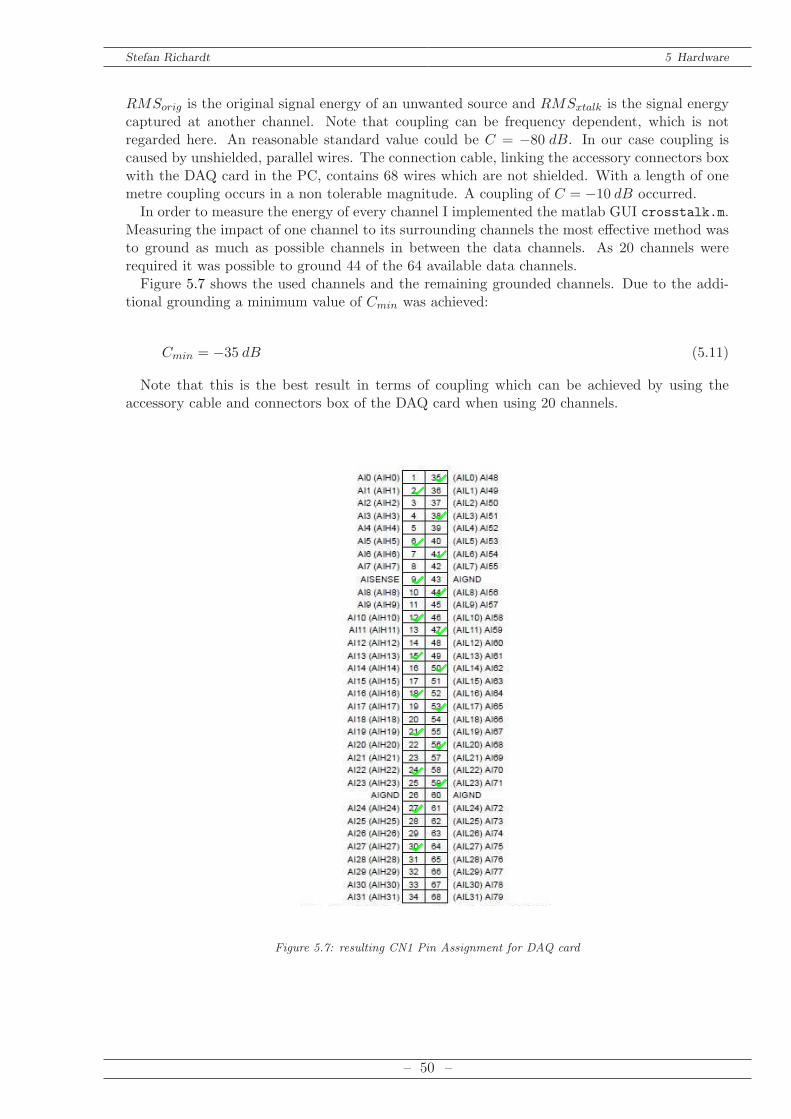
Stefan Richardt 5 Hardware
RMSorig is the original signal energy of an unwanted source and RMSxtalk is the signal energycaptured at another channel. Note that coupling can be frequency dependent, which is notregarded here. An reasonable standard value could be C = −80 dB. In our case coupling iscaused by unshielded, parallel wires. The connection cable, linking the accessory connectors boxwith the DAQ card in the PC, contains 68 wires which are not shielded. With a length of onemetre coupling occurs in a non tolerable magnitude. A coupling of C = −10 dB occurred.In order to measure the energy of every channel I implemented the matlab GUI crosstalk.m.
Measuring the impact of one channel to its surrounding channels the most effective method wasto ground as much as possible channels in between the data channels. As 20 channels wererequired it was possible to ground 44 of the 64 available data channels.Figure 5.7 shows the used channels and the remaining grounded channels. Due to the addi-
tional grounding a minimum value of Cmin was achieved:
Cmin = −35 dB (5.11)
Note that this is the best result in terms of coupling which can be achieved by using theaccessory cable and connectors box of the DAQ card when using 20 channels.
Figure 5.7: resulting CN1 Pin Assignment for DAQ card
– 50 –
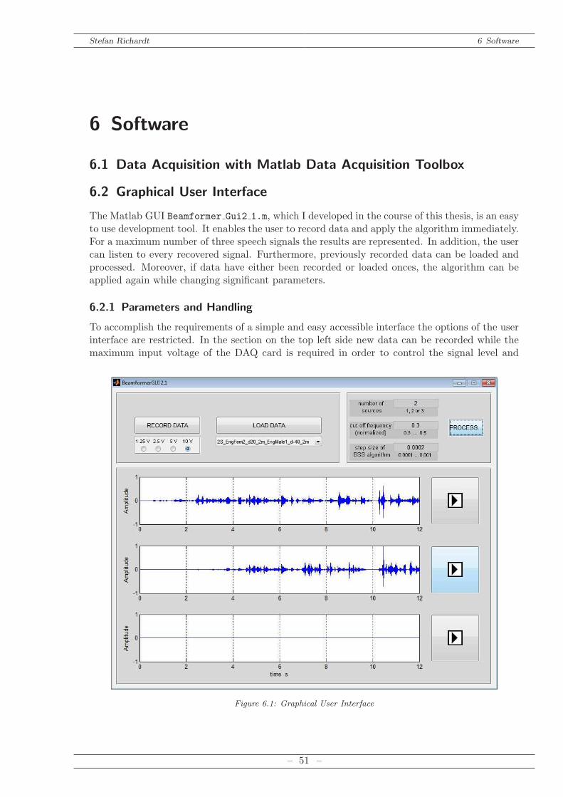
Stefan Richardt 6 Software
6 Software
6.1 Data Acquisition with Matlab Data Acquisition Toolbox
6.2 Graphical User Interface
The Matlab GUI Beamformer Gui2 1.m, which I developed in the course of this thesis, is an easyto use development tool. It enables the user to record data and apply the algorithm immediately.For a maximum number of three speech signals the results are represented. In addition, the usercan listen to every recovered signal. Furthermore, previously recorded data can be loaded andprocessed. Moreover, if data have either been recorded or loaded onces, the algorithm can beapplied again while changing significant parameters.
6.2.1 Parameters and Handling
To accomplish the requirements of a simple and easy accessible interface the options of the userinterface are restricted. In the section on the top left side new data can be recorded while themaximum input voltage of the DAQ card is required in order to control the signal level and
Figure 6.1: Graphical User Interface
– 51 –
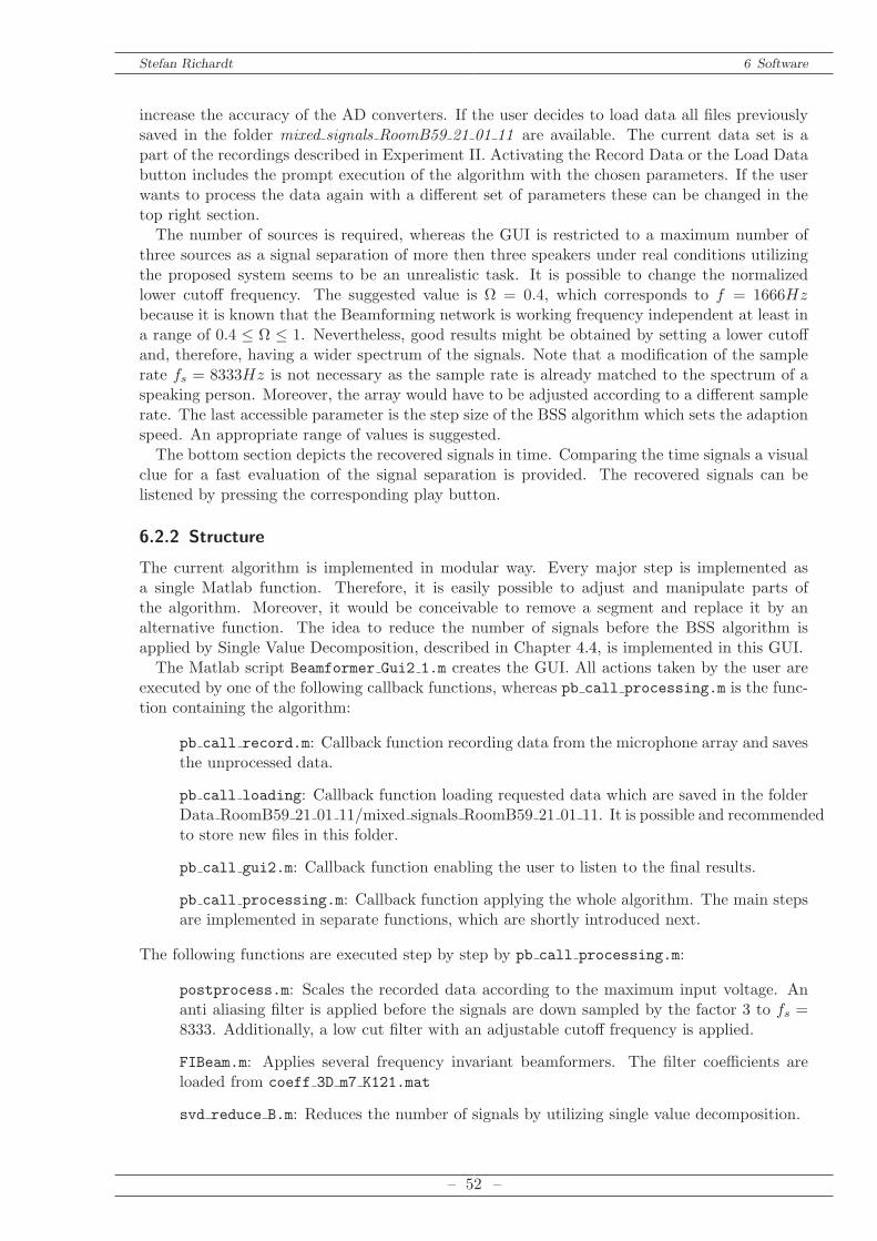
Stefan Richardt 6 Software
increase the accuracy of the AD converters. If the user decides to load data all files previouslysaved in the folder mixed signals RoomB59 21 01 11 are available. The current data set is apart of the recordings described in Experiment II. Activating the Record Data or the Load Databutton includes the prompt execution of the algorithm with the chosen parameters. If the userwants to process the data again with a different set of parameters these can be changed in thetop right section.The number of sources is required, whereas the GUI is restricted to a maximum number of
three sources as a signal separation of more then three speakers under real conditions utilizingthe proposed system seems to be an unrealistic task. It is possible to change the normalizedlower cutoff frequency. The suggested value is Ω = 0.4, which corresponds to f = 1666Hzbecause it is known that the Beamforming network is working frequency independent at least ina range of 0.4 ≤ Ω ≤ 1. Nevertheless, good results might be obtained by setting a lower cutoffand, therefore, having a wider spectrum of the signals. Note that a modification of the samplerate fs = 8333Hz is not necessary as the sample rate is already matched to the spectrum of aspeaking person. Moreover, the array would have to be adjusted according to a different samplerate. The last accessible parameter is the step size of the BSS algorithm which sets the adaptionspeed. An appropriate range of values is suggested.The bottom section depicts the recovered signals in time. Comparing the time signals a visual
clue for a fast evaluation of the signal separation is provided. The recovered signals can belistened by pressing the corresponding play button.
6.2.2 Structure
The current algorithm is implemented in modular way. Every major step is implemented asa single Matlab function. Therefore, it is easily possible to adjust and manipulate parts ofthe algorithm. Moreover, it would be conceivable to remove a segment and replace it by analternative function. The idea to reduce the number of signals before the BSS algorithm isapplied by Single Value Decomposition, described in Chapter 4.4, is implemented in this GUI.The Matlab script Beamformer Gui2 1.m creates the GUI. All actions taken by the user are
executed by one of the following callback functions, whereas pb call processing.m is the func-tion containing the algorithm:
pb call record.m: Callback function recording data from the microphone array and savesthe unprocessed data.
pb call loading: Callback function loading requested data which are saved in the folderData RoomB59 21 01 11/mixed signals RoomB59 21 01 11. It is possible and recommendedto store new files in this folder.
pb call gui2.m: Callback function enabling the user to listen to the final results.
pb call processing.m: Callback function applying the whole algorithm. The main stepsare implemented in separate functions, which are shortly introduced next.
The following functions are executed step by step by pb call processing.m:
postprocess.m: Scales the recorded data according to the maximum input voltage. Ananti aliasing filter is applied before the signals are down sampled by the factor 3 to fs =8333. Additionally, a low cut filter with an adjustable cutoff frequency is applied.
FIBeam.m: Applies several frequency invariant beamformers. The filter coefficients areloaded from coeff 3D m7 K121.mat
svd reduce B.m: Reduces the number of signals by utilizing single value decomposition.
– 52 –
Stefan Richardt 6 Software
BSS.m: A blind source seperation algorithm based on the natural gradient algorithm isapplied.
reconstruct singnal.m: Reconstructs the signals with the coefficients estimated by theBSS algorithm. The current set of coefficients is utilized. The recovered signals are nor-malized.
Moreover, the GUI requires a few additional functions: norm signal.m, design lowcut.m,
getfilenames.m. The filter coefficients for the anti aliasing filter are loaded from AA fs24999.mat
whereas the coefficients for the beamforming network are loaded from coeff 3D m7 K121.mat.Both files could be replaced if, for example, a different filter design shall be tested.Due to the fact that the algorithm is implemented separately from the interface it is possible
to develop new algorithms while using the same framework. The algorithm, implemented in amodular way, enables the user to change or replace parts quite easily in order to observe theresulting signals. On this account, this application is supposed to be used as basis for furtherdevelopment.
– 53 –

Stefan Richardt 6 Software
Part III
Results
– 54 –
Stefan Richardt 7 Experiments
7 Experiments
7.1 Experiment I
The first experiment was accomplished in a non reverberant environment. For that reason, weutilized the anechoic chamber in the Portobello Centre of the University of Sheffield. Withrespect to errors caused by curved waveforms the distance from the source to the microphonearray was chosen with r = 6 m. For a more detailed discussion of this problem please seeChapter 7.3. With a microphone number M = 19 and a distance of two adjoining microphonesd = 0.0408 m the dimension of the array was a = 0.7344 m. The microphone array and thesource were located at the same height. As we had a non reverberant environment, meaninga single path scenario, we were allowed to turn the array in order to change the DOA angleinstead of moving the source.
7.1.1 Experiment I a
First and foremost the purpose of this measurement was to review the performance of thebeamformer. A customary loudspeaker was utilized as source. The source signal was whiteGaussian noise. Applying the noise from a DOA angle in a range from 0 ≤ θ ≤ 90 with aresolution of 5 we are able to calculate the beam pattern later on.
Figure 7.1: Microphone array in anechoic chamber
– 55 –
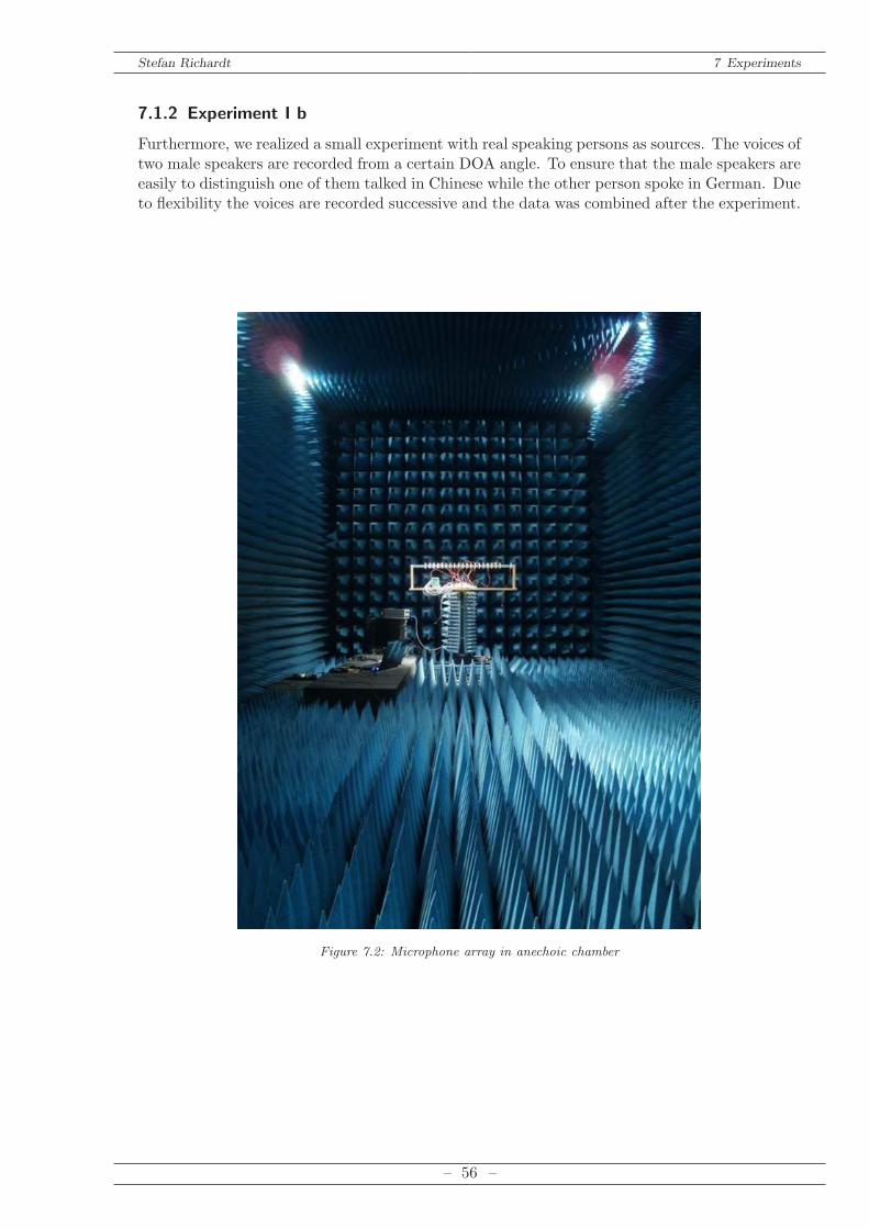
Stefan Richardt 7 Experiments
7.1.2 Experiment I b
Furthermore, we realized a small experiment with real speaking persons as sources. The voices oftwo male speakers are recorded from a certain DOA angle. To ensure that the male speakers areeasily to distinguish one of them talked in Chinese while the other person spoke in German. Dueto flexibility the voices are recorded successive and the data was combined after the experiment.
Figure 7.2: Microphone array in anechoic chamber
– 56 –
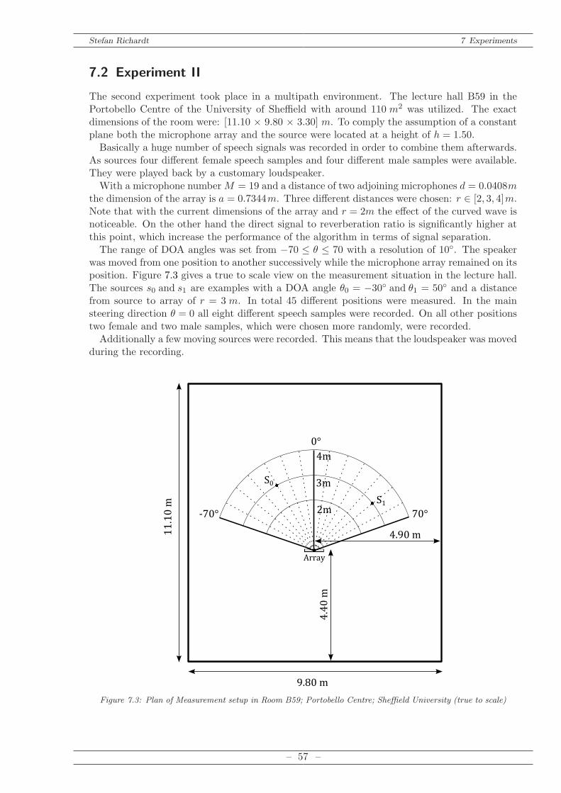
Stefan Richardt 7 Experiments
7.2 Experiment II
The second experiment took place in a multipath environment. The lecture hall B59 in thePortobello Centre of the University of Sheffield with around 110 m2 was utilized. The exactdimensions of the room were: [11.10 × 9.80 × 3.30] m. To comply the assumption of a constantplane both the microphone array and the source were located at a height of h = 1.50.Basically a huge number of speech signals was recorded in order to combine them afterwards.
As sources four different female speech samples and four different male samples were available.They were played back by a customary loudspeaker.With a microphone numberM = 19 and a distance of two adjoining microphones d = 0.0408m
the dimension of the array is a = 0.7344m. Three different distances were chosen: r ∈ [2, 3, 4]m.Note that with the current dimensions of the array and r = 2m the effect of the curved wave isnoticeable. On the other hand the direct signal to reverberation ratio is significantly higher atthis point, which increase the performance of the algorithm in terms of signal separation.The range of DOA angles was set from −70 ≤ θ ≤ 70 with a resolution of 10. The speaker
was moved from one position to another successively while the microphone array remained on itsposition. Figure 7.3 gives a true to scale view on the measurement situation in the lecture hall.The sources s0 and s1 are examples with a DOA angle θ0 = −30 and θ1 = 50 and a distancefrom source to array of r = 3 m. In total 45 different positions were measured. In the mainsteering direction θ = 0 all eight different speech samples were recorded. On all other positionstwo female and two male samples, which were chosen more randomly, were recorded.Additionally a few moving sources were recorded. This means that the loudspeaker was moved
during the recording.
0°
70°-70°
4m
3m
2m
S0
S1
Array
4.40m
4.90m11.10m
9.80m
Figure 7.3: Plan of Measurement setup in Room B59; Portobello Centre; Sheffield University (true to scale)
– 57 –
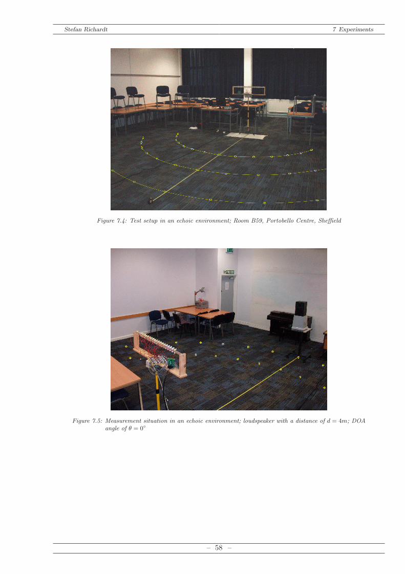
Stefan Richardt 7 Experiments
Figure 7.4: Test setup in an echoic environment; Room B59, Portobello Centre, Sheffield
Figure 7.5: Measurement situation in an echoic environment; loudspeaker with a distance of d = 4m; DOAangle of θ = 0
– 58 –
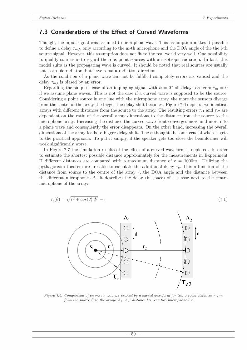
Stefan Richardt 7 Experiments
7.3 Considerations of the Effect of Curved Waveforms
Though, the input signal was assumed to be a plane wave. This assumption makes it possibleto define a delay τm,l, only according to the m-th microphone and the DOA angle of the the l-thsource signal. However, this assumption does not fit to the real world very well. One possibilityto qualify sources is to regard them as point sources with an isotropic radiation. In fact, thismodel suits as the propagating wave is curved. It should be noted that real sources are usuallynot isotropic radiators but have a main radiation direction.As the condition of a plane wave can not be fulfilled completely errors are caused and the
delay τm,l is biased by an error.Regarding the simplest case of an impinging signal with φ = 0 all delays are zero τm = 0
if we assume plane waves. This is not the case if a curved wave is supposed to be the source.Considering a point source in one line with the microphone array, the more the sensors divergefrom the centre of the array the bigger the delay shift becomes. Figure 7.6 depicts two identicalarrays with different distances from the source to the array. The resulting errors τe1 and τe2 aredependent on the ratio of the overall array dimensions to the distance from the source to themicrophone array. Increasing the distance the curved wave front converges more and more intoa plane wave and consequently the error disappears. On the other hand, increasing the overalldimensions of the array leads to bigger delay shift. These thoughts become crucial when it getsto the practical approach. To put it simply, if the speaker gets too close the beamformer willwork significantly worse.In Figure 7.7 the simulation results of the effect of a curved waveform is depicted. In order
to estimate the shortest possible distance approximately for the measurements in ExperimentII different distances are compared with a maximum distance of r = 1000m. Utilizing thepythagoreom theorem we are able to calculate the additional delay τe. It is a function of thedistance from source to the centre of the array r, the DOA angle and the distance betweenthe different microphones d. It describes the delay (in space) of a sensor next to the centremicrophone of the array:
τe(θ) =√
r2 + cos(θ) d2 − r (7.1)
Figure 7.6: Comparison of errors τe1 and τe2 evolved by a curved waveform for two arrays; distances r1, r2from the source S to the arrays A1, A2; distance between two microphones: d
– 59 –
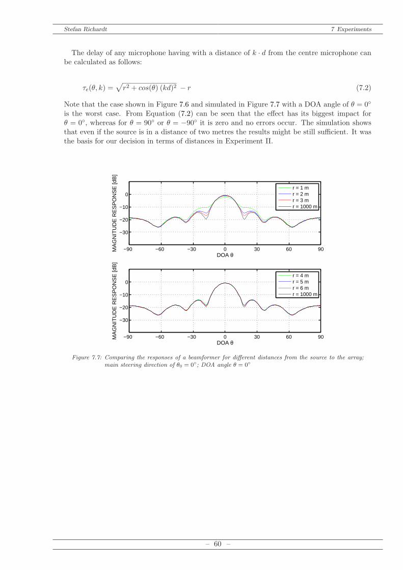
Stefan Richardt 7 Experiments
The delay of any microphone having with a distance of k · d from the centre microphone canbe calculated as follows:
τe(θ, k) =√
r2 + cos(θ) (kd)2 − r (7.2)
Note that the case shown in Figure 7.6 and simulated in Figure 7.7 with a DOA angle of θ = 0
is the worst case. From Equation (7.2) can be seen that the effect has its biggest impact forθ = 0, whereas for θ = 90 or θ = −90 it is zero and no errors occur. The simulation showsthat even if the source is in a distance of two metres the results might be still sufficient. It wasthe basis for our decision in terms of distances in Experiment II.
−90 −60 −30 0 30 60 90
−30
−20
−10
0
DOA θ
MA
GN
ITU
DE
RE
SP
ON
SE
[dB
]
r = 1 mr = 2 mr = 3 mr = 1000 m
−90 −60 −30 0 30 60 90
−30
−20
−10
0
DOA θ
MA
GN
ITU
DE
RE
SP
ON
SE
[dB
]
r = 4 mr = 5 mr = 6 mr = 1000 m
Figure 7.7: Comparing the responses of a beamformer for different distances from the source to the array;main steering direction of θ0 = 0; DOA angle θ = 0
– 60 –
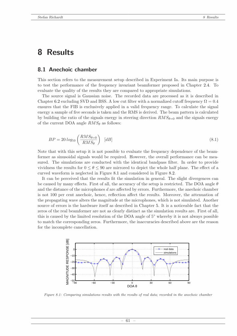
Stefan Richardt 8 Results
8 Results
8.1 Anechoic chamber
This section refers to the measurement setup described in Experiment Ia. Its main purpose isto test the performance of the frequency invariant beamformer proposed in Chapter 2.4. Toevaluate the quality of the results they are compared to appropriate simulations.The source signal is Gaussian noise. The recorded data are processed as it is described in
Chapter 6.2 excluding SVD and BSS. A low cut filter with a normalized cutoff frequency Ω = 0.4ensures that the FIB is exclusively applied in a valid frequency range. To calculate the signalenergy a sample of five seconds is taken and the RMS is derived. The beam pattern is calculatedby building the ratio of the signals energy in steering direction RMSθ=0 and the signals energyof the current DOA angle RMSθ as follows:
BP = 20 log10
(RMSθ=0
RMSθ
)
[dB] (8.1)
Note that with this setup it is not possible to evaluate the frequency dependence of the beam-former as sinusoidal signals would be required. However, the overall performance can be mea-sured. The simulations are conducted with the identical bandpass filter. In order to providevividness the results for 0 ≤ θ ≤ 90 are mirrored to depict the whole half plane. The effect of acurved waveform is neglected in Figure 8.1 and considered in Figure 8.2.It can be perceived that the results fit the simulation in general. The slight divergences can
be caused by many effects. First of all, the accuracy of the setup is restricted. The DOA angle θand the distance of the microphones d are affected by errors. Furthermore, the anechoic chamberis not 100 per cent anechoic, hence, reflection affect the results. Moreover, the attenuation ofthe propagating wave alters the magnitude at the microphones, which is not simulated. Anothersource of errors is the hardware itself as described in Chapter 5. It is a noticeable fact that thezeros of the real beamformer are not as clearly distinct as the simulation results are. First of all,this is caused by the limited resolution of the DOA angle of 5 whereby it is not always possibleto match the corresponding zeros. Furthermore, the inaccuracies described above are the reasonfor the incomplete cancellation.
−90 −60 −30 0 30 60 90−50
−40
−30
−20
−10
0
DOA θ
MA
GN
ITU
DE
RE
SP
ON
SE
[dB
]
real datasimulations
Figure 8.1: Comparing simulations results with the results of real data; recorded in the anechoic chamber
– 61 –
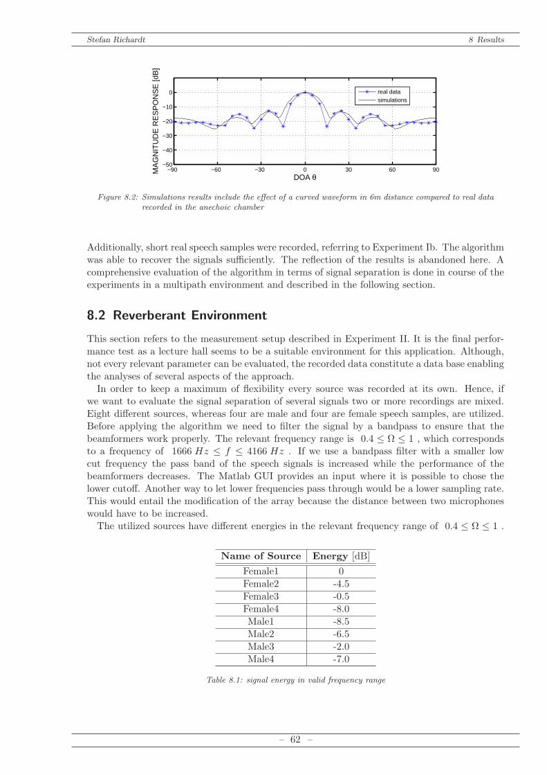
Stefan Richardt 8 Results
−90 −60 −30 0 30 60 90−50
−40
−30
−20
−10
0
DOA θ
MA
GN
ITU
DE
RE
SP
ON
SE
[dB
]
real datasimulations
Figure 8.2: Simulations results include the effect of a curved waveform in 6m distance compared to real datarecorded in the anechoic chamber
Additionally, short real speech samples were recorded, referring to Experiment Ib. The algorithmwas able to recover the signals sufficiently. The reflection of the results is abandoned here. Acomprehensive evaluation of the algorithm in terms of signal separation is done in course of theexperiments in a multipath environment and described in the following section.
8.2 Reverberant Environment
This section refers to the measurement setup described in Experiment II. It is the final perfor-mance test as a lecture hall seems to be a suitable environment for this application. Although,not every relevant parameter can be evaluated, the recorded data constitute a data base enablingthe analyses of several aspects of the approach.In order to keep a maximum of flexibility every source was recorded at its own. Hence, if
we want to evaluate the signal separation of several signals two or more recordings are mixed.Eight different sources, whereas four are male and four are female speech samples, are utilized.Before applying the algorithm we need to filter the signal by a bandpass to ensure that thebeamformers work properly. The relevant frequency range is 0.4 ≤ Ω ≤ 1 , which correspondsto a frequency of 1666 Hz ≤ f ≤ 4166 Hz . If we use a bandpass filter with a smaller lowcut frequency the pass band of the speech signals is increased while the performance of thebeamformers decreases. The Matlab GUI provides an input where it is possible to chose thelower cutoff. Another way to let lower frequencies pass through would be a lower sampling rate.This would entail the modification of the array because the distance between two microphoneswould have to be increased.The utilized sources have different energies in the relevant frequency range of 0.4 ≤ Ω ≤ 1 .
Name of Source Energy [dB]
Female1 0Female2 -4.5Female3 -0.5Female4 -8.0Male1 -8.5Male2 -6.5Male3 -2.0Male4 -7.0
Table 8.1: signal energy in valid frequency range
– 62 –
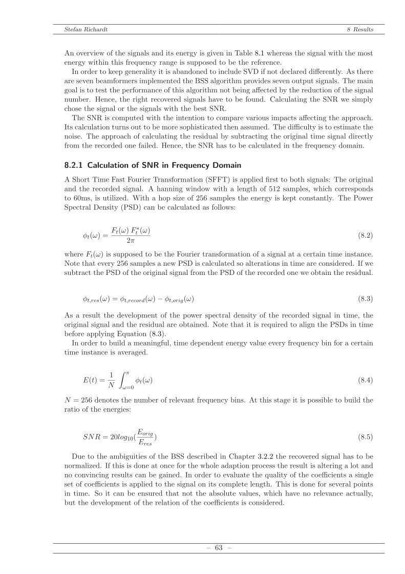
Stefan Richardt 8 Results
An overview of the signals and its energy is given in Table 8.1 whereas the signal with the mostenergy within this frequency range is supposed to be the reference.In order to keep generality it is abandoned to include SVD if not declared differently. As there
are seven beamformers implemented the BSS algorithm provides seven output signals. The maingoal is to test the performance of this algorithm not being affected by the reduction of the signalnumber. Hence, the right recovered signals have to be found. Calculating the SNR we simplychose the signal or the signals with the best SNR.The SNR is computed with the intention to compare various impacts affecting the approach.
Its calculation turns out to be more sophisticated then assumed. The difficulty is to estimate thenoise. The approach of calculating the residual by subtracting the original time signal directlyfrom the recorded one failed. Hence, the SNR has to be calculated in the frequency domain.
8.2.1 Calculation of SNR in Frequency Domain
A Short Time Fast Fourier Transformation (SFFT) is applied first to both signals: The originaland the recorded signal. A hanning window with a length of 512 samples, which correspondsto 60ms, is utilized. With a hop size of 256 samples the energy is kept constantly. The PowerSpectral Density (PSD) can be calculated as follows:
φt(ω) =Ft(ω) F
∗
t (ω)
2π(8.2)
where Ft(ω) is supposed to be the Fourier transformation of a signal at a certain time instance.Note that every 256 samples a new PSD is calculated so alterations in time are considered. If wesubtract the PSD of the original signal from the PSD of the recorded one we obtain the residual.
φt,res(ω) = φt,record(ω)− φt,orig(ω) (8.3)
As a result the development of the power spectral density of the recorded signal in time, theoriginal signal and the residual are obtained. Note that it is required to align the PSDs in timebefore applying Equation (8.3).In order to build a meaningful, time dependent energy value every frequency bin for a certain
time instance is averaged.
E(t) =1
N
∫ π
ω=0φt(ω) (8.4)
N = 256 denotes the number of relevant frequency bins. At this stage it is possible to build theratio of the energies:
SNR = 20log10(Eorig
Eres) (8.5)
Due to the ambiguities of the BSS described in Chapter 3.2.2 the recovered signal has to benormalized. If this is done at once for the whole adaption process the result is altering a lot andno convincing results can be gained. In order to evaluate the quality of the coefficients a singleset of coefficients is applied to the signal on its complete length. This is done for several pointsin time. So it can be ensured that not the absolute values, which have no relevance actually,but the development of the relation of the coefficients is considered.
– 63 –
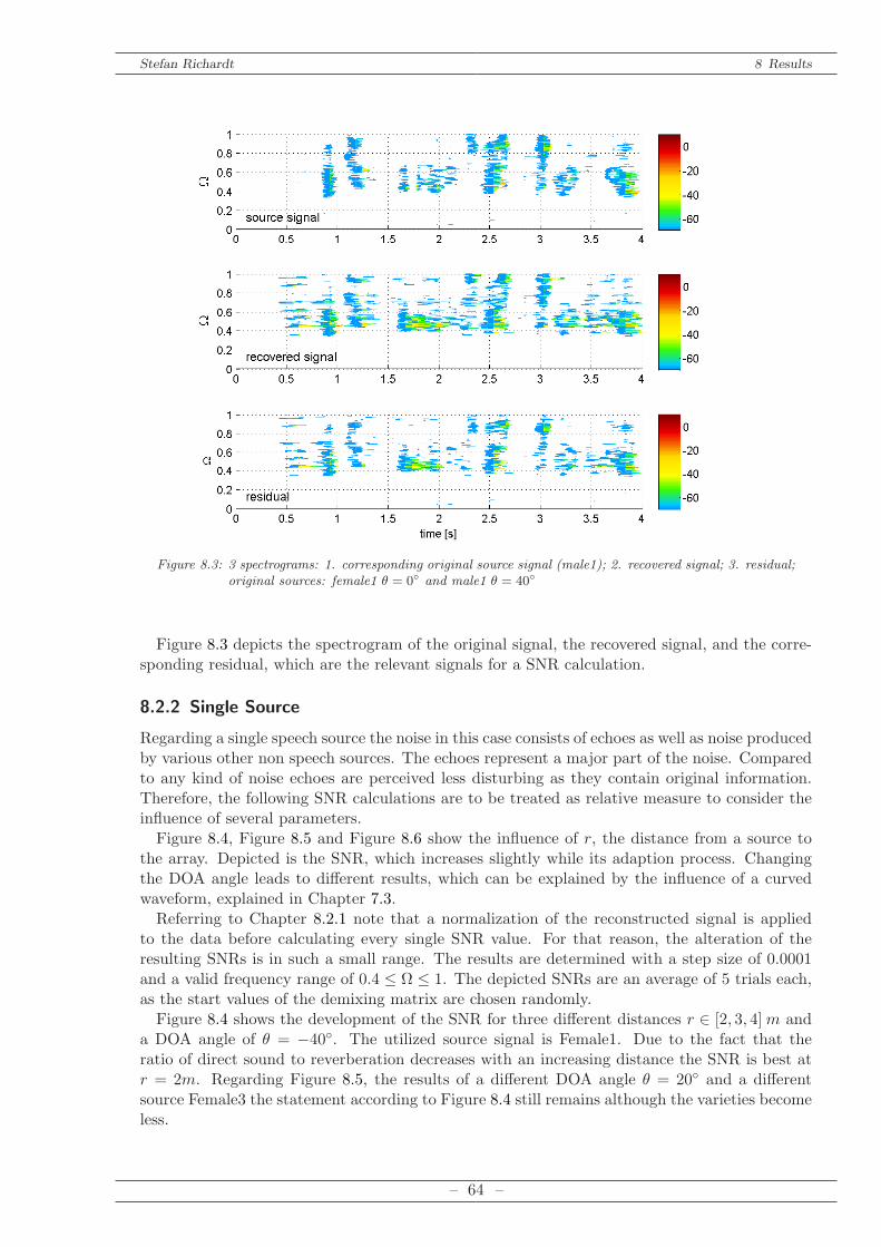
Stefan Richardt 8 Results
Figure 8.3: 3 spectrograms: 1. corresponding original source signal (male1); 2. recovered signal; 3. residual;original sources: female1 θ = 0 and male1 θ = 40
Figure 8.3 depicts the spectrogram of the original signal, the recovered signal, and the corre-sponding residual, which are the relevant signals for a SNR calculation.
8.2.2 Single Source
Regarding a single speech source the noise in this case consists of echoes as well as noise producedby various other non speech sources. The echoes represent a major part of the noise. Comparedto any kind of noise echoes are perceived less disturbing as they contain original information.Therefore, the following SNR calculations are to be treated as relative measure to consider theinfluence of several parameters.Figure 8.4, Figure 8.5 and Figure 8.6 show the influence of r, the distance from a source to
the array. Depicted is the SNR, which increases slightly while its adaption process. Changingthe DOA angle leads to different results, which can be explained by the influence of a curvedwaveform, explained in Chapter 7.3.Referring to Chapter 8.2.1 note that a normalization of the reconstructed signal is applied
to the data before calculating every single SNR value. For that reason, the alteration of theresulting SNRs is in such a small range. The results are determined with a step size of 0.0001and a valid frequency range of 0.4 ≤ Ω ≤ 1. The depicted SNRs are an average of 5 trials each,as the start values of the demixing matrix are chosen randomly.Figure 8.4 shows the development of the SNR for three different distances r ∈ [2, 3, 4]m and
a DOA angle of θ = −40. The utilized source signal is Female1. Due to the fact that theratio of direct sound to reverberation decreases with an increasing distance the SNR is best atr = 2m. Regarding Figure 8.5, the results of a different DOA angle θ = 20 and a differentsource Female3 the statement according to Figure 8.4 still remains although the varieties becomeless.
– 64 –
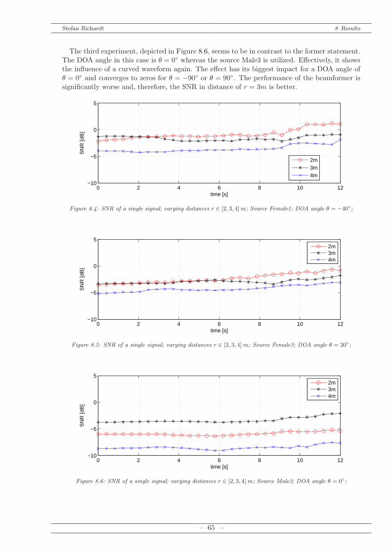
Stefan Richardt 8 Results
The third experiment, depicted in Figure 8.6, seems to be in contrast to the former statement.The DOA angle in this case is θ = 0 whereas the source Male3 is utilized. Effectively, it showsthe influence of a curved waveform again. The effect has its biggest impact for a DOA angle ofθ = 0 and converges to zeros for θ = −90 or θ = 90. The performance of the beamformer issignificantly worse and, therefore, the SNR in distance of r = 3m is better.
0 2 4 6 8 10 12−10
−5
0
5
SN
R [d
B]
time [s]
2m3m4m
Figure 8.4: SNR of a single signal; varying distances r ∈ [2, 3, 4]m; Source Female1; DOA angle θ = −40;
0 2 4 6 8 10 12−10
−5
0
5
SN
R [d
B]
time [s]
2m3m4m
Figure 8.5: SNR of a single signal; varying distances r ∈ [2, 3, 4]m; Source Female3; DOA angle θ = 20;
0 2 4 6 8 10 12−10
−5
0
5
SN
R [d
B]
time [s]
2m3m4m
Figure 8.6: SNR of a single signal; varying distances r ∈ [2, 3, 4]m; Source Male3; DOA angle θ = 0;
– 65 –
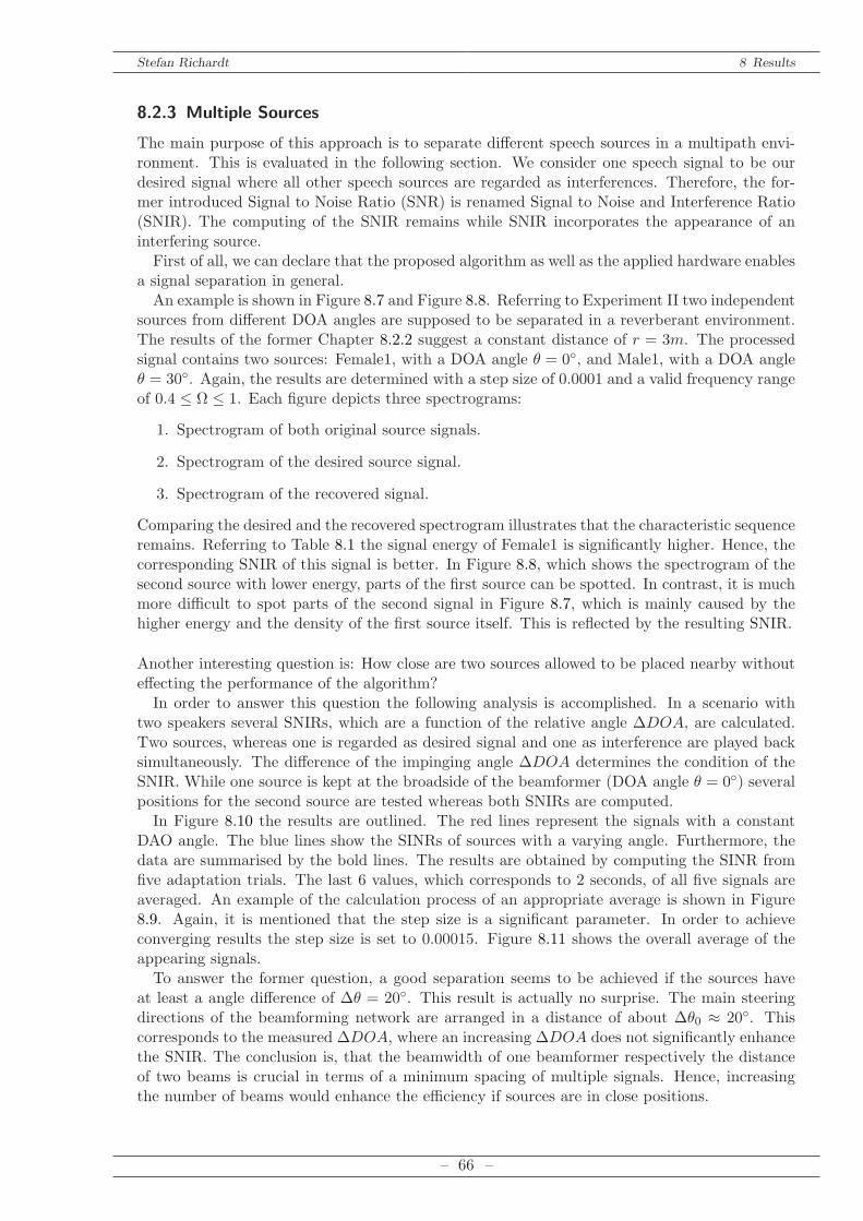
Stefan Richardt 8 Results
8.2.3 Multiple Sources
The main purpose of this approach is to separate different speech sources in a multipath envi-ronment. This is evaluated in the following section. We consider one speech signal to be ourdesired signal where all other speech sources are regarded as interferences. Therefore, the for-mer introduced Signal to Noise Ratio (SNR) is renamed Signal to Noise and Interference Ratio(SNIR). The computing of the SNIR remains while SNIR incorporates the appearance of aninterfering source.First of all, we can declare that the proposed algorithm as well as the applied hardware enables
a signal separation in general.An example is shown in Figure 8.7 and Figure 8.8. Referring to Experiment II two independent
sources from different DOA angles are supposed to be separated in a reverberant environment.The results of the former Chapter 8.2.2 suggest a constant distance of r = 3m. The processedsignal contains two sources: Female1, with a DOA angle θ = 0, and Male1, with a DOA angleθ = 30. Again, the results are determined with a step size of 0.0001 and a valid frequency rangeof 0.4 ≤ Ω ≤ 1. Each figure depicts three spectrograms:
1. Spectrogram of both original source signals.
2. Spectrogram of the desired source signal.
3. Spectrogram of the recovered signal.
Comparing the desired and the recovered spectrogram illustrates that the characteristic sequenceremains. Referring to Table 8.1 the signal energy of Female1 is significantly higher. Hence, thecorresponding SNIR of this signal is better. In Figure 8.8, which shows the spectrogram of thesecond source with lower energy, parts of the first source can be spotted. In contrast, it is muchmore difficult to spot parts of the second signal in Figure 8.7, which is mainly caused by thehigher energy and the density of the first source itself. This is reflected by the resulting SNIR.
Another interesting question is: How close are two sources allowed to be placed nearby withouteffecting the performance of the algorithm?In order to answer this question the following analysis is accomplished. In a scenario with
two speakers several SNIRs, which are a function of the relative angle ∆DOA, are calculated.Two sources, whereas one is regarded as desired signal and one as interference are played backsimultaneously. The difference of the impinging angle ∆DOA determines the condition of theSNIR. While one source is kept at the broadside of the beamformer (DOA angle θ = 0) severalpositions for the second source are tested whereas both SNIRs are computed.In Figure 8.10 the results are outlined. The red lines represent the signals with a constant
DAO angle. The blue lines show the SINRs of sources with a varying angle. Furthermore, thedata are summarised by the bold lines. The results are obtained by computing the SINR fromfive adaptation trials. The last 6 values, which corresponds to 2 seconds, of all five signals areaveraged. An example of the calculation process of an appropriate average is shown in Figure8.9. Again, it is mentioned that the step size is a significant parameter. In order to achieveconverging results the step size is set to 0.00015. Figure 8.11 shows the overall average of theappearing signals.To answer the former question, a good separation seems to be achieved if the sources have
at least a angle difference of ∆θ = 20. This result is actually no surprise. The main steeringdirections of the beamforming network are arranged in a distance of about ∆θ0 ≈ 20. Thiscorresponds to the measured ∆DOA, where an increasing ∆DOA does not significantly enhancethe SNIR. The conclusion is, that the beamwidth of one beamformer respectively the distanceof two beams is crucial in terms of a minimum spacing of multiple signals. Hence, increasingthe number of beams would enhance the efficiency if sources are in close positions.
– 66 –

Stefan Richardt 8 Results
In order to evaluate the improvement of our algorithm, the SNIR of a single microphone iscalculated. The computation is conducted in the same way as it is done to assess the results ofthe algorithm. Both are compared in Figure 8.11. A clear improvement can be seen. We cancalculate the difference between the SNIRs with and without using the algorithm as follows:
∆SNIR = SNIRalgo − SNIRmic (8.6)
where SNIRalgo is the signal to noise and interference ratio when the algorithm is applied andSNIRmic the calculated measure for a single microphone. Figure 8.12 shows the improvementin terms of SNIR for the case of two speaking persons in a distance of r = 3m. The followingoverall enhancement of ∆SNIR can be achieved when neglecting values of ∆DOA ∈ [−10, 0, 10]:
∆SNIR ≈ 9 dB (8.7)
– 67 –
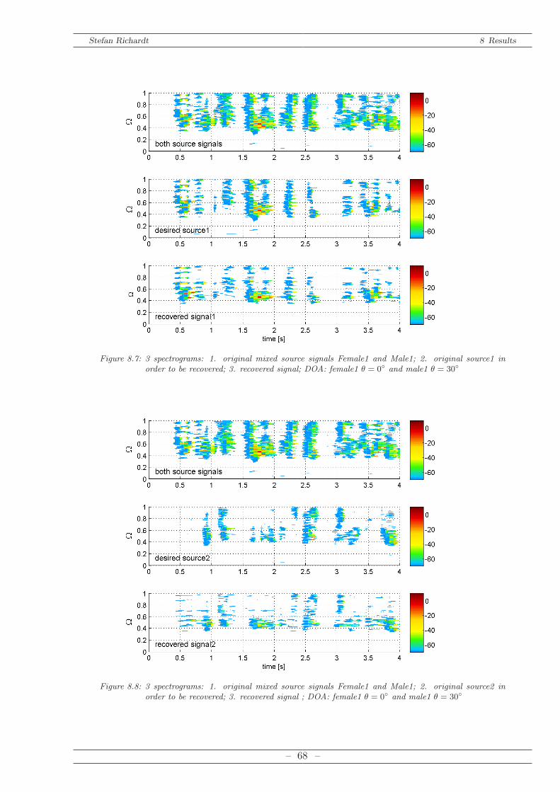
Stefan Richardt 8 Results
Figure 8.7: 3 spectrograms: 1. original mixed source signals Female1 and Male1; 2. original source1 inorder to be recovered; 3. recovered signal; DOA: female1 θ = 0 and male1 θ = 30
Figure 8.8: 3 spectrograms: 1. original mixed source signals Female1 and Male1; 2. original source2 inorder to be recovered; 3. recovered signal ; DOA: female1 θ = 0 and male1 θ = 30
– 68 –
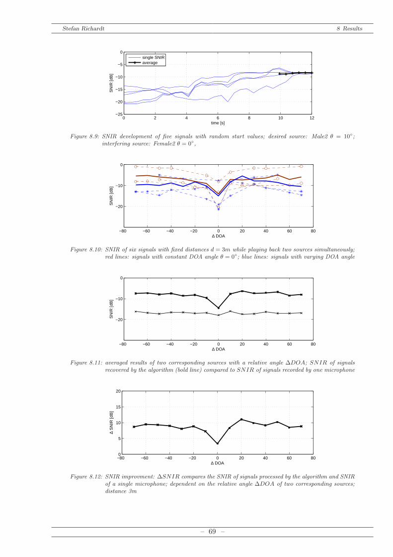
Stefan Richardt 8 Results
0 2 4 6 8 10 12−25
−20
−15
−10
−5
0
SN
IR [d
B]
time [s]
single SNIRaverage
Figure 8.9: SNIR development of five signals with random start values; desired source: Male2 θ = 10;interfering source: Female2 θ = 0,
−80 −60 −40 −20 0 20 40 60 80
−20
−10
0
∆ DOA
SN
IR [d
B]
Figure 8.10: SNIR of six signals with fixed distances d = 3m while playing back two sources simultaneously;red lines: signals with constant DOA angle θ = 0; blue lines: signals with varying DOA angle
−80 −60 −40 −20 0 20 40 60 80
−20
−10
0
∆ DOA
SN
IR [d
B]
Figure 8.11: averaged results of two corresponding sources with a relative angle ∆DOA; SNIR of signalsrecovered by the algorithm (bold line) compared to SNIR of signals recorded by one microphone
−80 −60 −40 −20 0 20 40 60 800
5
10
15
20
∆ DOA
∆ S
NIR
[dB
]
Figure 8.12: SNIR improvment: ∆SNIR compares the SNIR of signals processed by the algorithm and SNIRof a single microphone; dependent on the relative angle ∆DOA of two corresponding sources;distance 3m
– 69 –
Stefan Richardt 9 Conclusion and Prospects
9 Conclusion and Prospects
The scope of this work was to build a system that enables the user to apply the proposedalgorithm and to apply access to the results immediately. As a result a fully functional hardwaresetup as well as an easy to use Matlab GUI was developed.
9.1 Conclusion
It is shown that the proposed algorithm can be applied under real conditions in a reverberantenvironment whereby the limits of the approach are exposed. The performance of the systemis signal and environment dependent. The experiment in a lecture hall demonstrates the de-pendency on the source location and the relative location of multiple sources in detail. Theperformance decreases with an increasing ratio of reverberations to direct sound at the locationof the microphone array. Therefore, smaller rooms are unsuitable as the source location with aproper ratio can be in a very close position to the array. Noise or interfering signals which arenon directional can not be canceled by this algorithm. However, even if the issue of a multipathenvironment can not fully be solved, the system is capable to enhance the SNIR by suppressinginterfering sources effectively. Furthermore, the algorithm is able to cancel a small number ofreflected interferences, if the DOA angle does not match with the DOA angle of the desiredsource.The Matlab GUI Beamformer Gui2 1.m is a fully functional tool, enabling the user to easily
apply experiments in order to evaluate the performance of the algorithm. Due to its mod-ular structure it is suggested to modify or replace certain parts of the algorithm gaining animprovement of the approach.The single stages of the proposed algorithm can be modified separately. The FIB network
and the BSS algorithm are independent and work successively. Hence, a separate developmentis possible. If one of these parts is improved it can be replaced while retaining the other part.Besides, it is achievable to modify the BSS algorithm in order to recover different kinds of signals,as the applied approach is optimized in terms of speech separation. Thereby, an extension of thevalid frequency range of the FIB network would be desirable. Further to this approach, whichaims at a good speech discrimination, the frequency range is sufficient.Different from comparable beamforming systems a priori knowledge of the DOA is not re-
quired. Moreover, it should be possible to calculate the DOA angles of the desired sourcesby evaluating the corresponding set of coefficients. The only a priori knowledge needed is thenumber of sources L.Summarizing, the proposed system can be described as unconventional and valid approach in
order to separate several speech signals.
– 70 –

Stefan Richardt 9 Conclusion and Prospects
9.2 Prospects
The system is supposed to work in real time. To a certain level this requirement is complied.The computation of a certain recording can be performed in a shorter time than the lengths ofthis recording. The system shall be extended with the final goal of enabling the user to directlylisten to the results while one or more persons are speaking. Additionally, the optimization of thesystem can be further refined. A remaining question is if an increasing number of beamformersleads to a better performance. As block processing is required in order to replay the processeddata with a minimum delay it is suggested to abandon the SVD stage. Therefore, a modified BSSneeds to be implemented. Suggestions can be found in Chapter 4.4. Furthermore, the constraintsof the coefficients respectively the normalization of the signals could become a problem.In principle, the system including the hardware can be used as basis for a further development
of such a real time system. The data acquisition toolbox enables a direct data access in Matlab.It is recommended to implement a software being able to record and replay data virtuallysimultaneously while a simple FIR filter is applied. If such a application is doable, a block byblock implementation of the whole algorithm should be possible.Last but not least, I want to mention an alternative possibility of an online, Matlab-based
signal processing approach. In the course of the diploma thesis [Dietze, 2010], conducted atthe Graz University of Technology, a convincing concept, utilizing Matlab for real time dataprocessing is introduced. The Matlab-compatible software ‘playrec’ is used in order to achieveaccess to a standardized multichannel audio format such as ASIO (Audio Stream Input/Output),which is provided by a various number of sound cards. This, of course, would require professionalaudio equipment, which would solve the majority of the hardware caused problems on the otherhand.I hope that my work will be continued and contributes to the research and development
accomplished by the Department of Electronic and Electrical Engineering in Sheffield.
– 71 –
Stefan Richardt Bibliography
Bibliography
[Amari, 1999] Amari, C. (1999). Natural gradient learning for over- and under complete basesin ica. Neural Computation, 11:1875–1883.
[Benesty et al., 2008] Benesty, J., Chen, J., and Huang, Y. (2008). Microphone Array SignalProcessing. Springer.
[Cichocki and Amari, 2002] Cichocki, A. and Amari, S. (2002). Adaptive Blind Signal and ImageProcessing. John Wiley & Sons Ltd.
[Dietze, 2010] Dietze, B. M. (2010). Room response equalization and loudspeaker crossovernetworks. Master’s thesis, Graz, Technical University.
[Dollfuß, 2010] Dollfuß, P. (2010). Driving direction detection with microphone arrays. Master’sthesis, Graz, University of Technology.
[Hyvarinen et al., 2001] Hyvarinen, A., Karhunen, J., and Oja, E. (2001). Independent Compo-nent Analysis. John Wiley & Sons Ltd.
[Hyvarinen and Oja, 2000] Hyvarinen, A. and Oja, E. (2000). Indenpendent component analy-sis:algorithms and applications. Elsevier, Neural Networks, Vol.13:411–430.
[Joho et al., 2000] Joho, M., Mathis, H., and R., L. (2000). Overdetermined blind source sepa-ration: Using more sensors than source signals in a noisy mixture. Indenpendent ComponentAnalysis and Blind Source Seperation ICA, pages 81–86.
[Liu, 2010] Liu, W. (2010). Blind beamforming for multi-path wideband signals based on fre-quency invariant transformation. In Proc. 4th Int Communications, Control and Signal Pro-cessing (ISCCSP) Symp, pages 1–4.
[Liu and Mandic, 2005] Liu, W. and Mandic, D. P. (2005). Semi-blind source separation forconvolutive mixtures based on frequency invariant transformation. In Proc. IEEE Int. Conf.Acoustics, Speech, and Signal Processing (ICASSP ’05), volume 5.
[Liu and Weiss, 2008] Liu, W. and Weiss, S. (2008). Design of frequency invariant beamformersfor broadband arrays. Signal Processing IEEE, 56(2):855–860.
[Liu and Weiss, 2010] Liu, W. and Weiss, S. (2010). Wideband Beamforming: Concepts andTechniques. John Wiley & Sons Ltd.
[Oppenheim et al., 2004] Oppenheim, A., Schafer, R., and Book, J. (2004). Zeitdiskrete Sig-nalverarbeitung. Pearson Studium.
[Pape, 2005] Pape, L. (2005). Vergleich robuster beamformer arrays. Master’s thesis, Graz,Technical University.
[Sekiguchi and Karasawa, 2000] Sekiguchi, T. and Karasawa, Y. (2000). Wideband beamspaceadaptive array utilizing fir fan filters for multibeam forming. Signal Processing IEEE,48(1):277–284.
– 72 –

Stefan Richardt Bibliography
[Vary and Martin, 2006] Vary, P. and Martin, R. (2006). Digital Speech Transmission. JohnWiley & Sons Ltd.
[Williams, 1999] Williams, E. (1999). Fourier Acoustics; Sound Radiation and Nearfield Acous-tical Holography. Academic Press.
[Zhang et al., 1999] Zhang, L.-Q., Cichocki, A., and Amari, S. (1999). Natural gradient algo-rithm for blind separation of overdetermined mixture with additive noise. Signal ProcessingLetters IEEE, 6(11):293–295.
– 73 –