1

Direct Fatigue Damage Spectrum Calculation for a Shock Response Spectrum

By Tom Irvine

Email: tom@vibrationdata.com

June 25, 2014

_____________________________________________________________________________________

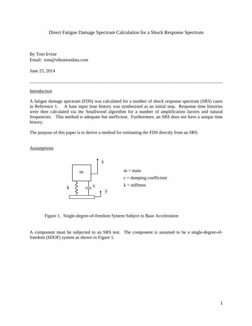
Introduction

A fatigue damage spectrum (FDS) was calculated for a number of shock response spectrum (SRS) cases

in Reference 1. A base input time history was synthesized as an initial step. Response time histories

were then calculated via the Smallwood algorithm for a number of amplification factors and natural

frequencies. This method is adequate but inefficient. Furthermore, an SRS does not have a unique time

history.

The purpose of this paper is to derive a method for estimating the FDS directly from an SRS.

Assumptions

Figure 1. Single-degree-of-freedom System Subject to Base Acceleration

A component must be subjected to an SRS test. The component is assumed to be a single-degree-of-

freedom (SDOF) system as shown in Figure 1.

m

k c

x

y

m = mass

c = damping coefficient

k = stiffness

2

Fatigue Damage Spectrum

A rainflow cycle count can be performed for each SDOF response for each natural frequency fn and

amplification factor Q of interest.

The fatigue damage spectrum (FDS) is calculated from the response rainflow cycles.

A relative damage index D is calculated using

i

m

1i

bi

nAD

(1)

where

iA is the response amplitude from the rainflow analysis

in is the corresponding number of cycles

b is the fatigue exponent

Note that the amplitude convention for this paper is: (peak-valley)/2.

The FDS expresses damage as a function of natural frequency with the Q and b values duly noted.

3

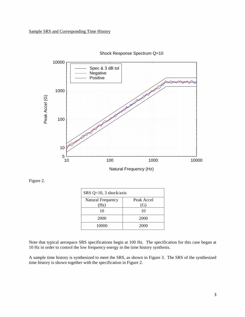
Sample SRS and Corresponding Time History

Figure 2.

SRS Q=10, 3 shock/axis

Natural Frequency

(Hz)

Peak Accel

(G)

10 10

2000 2000

10000 2000

Note that typical aerospace SRS specifications begin at 100 Hz. The specification for this case began at

10 Hz in order to control the low frequency energy in the time history synthesis.

A sample time history is synthesized to meet the SRS, as shown in Figure 3. The SRS of the synthesized

time history is shown together with the specification in Figure 2.

10

100

1000

10000

510 100 1000 10000

Spec & 3 dB tolNegativePositive

Natural Frequency (Hz)

Pe

ak A

cce

l (G

)

Shock Response Spectrum Q=10

4

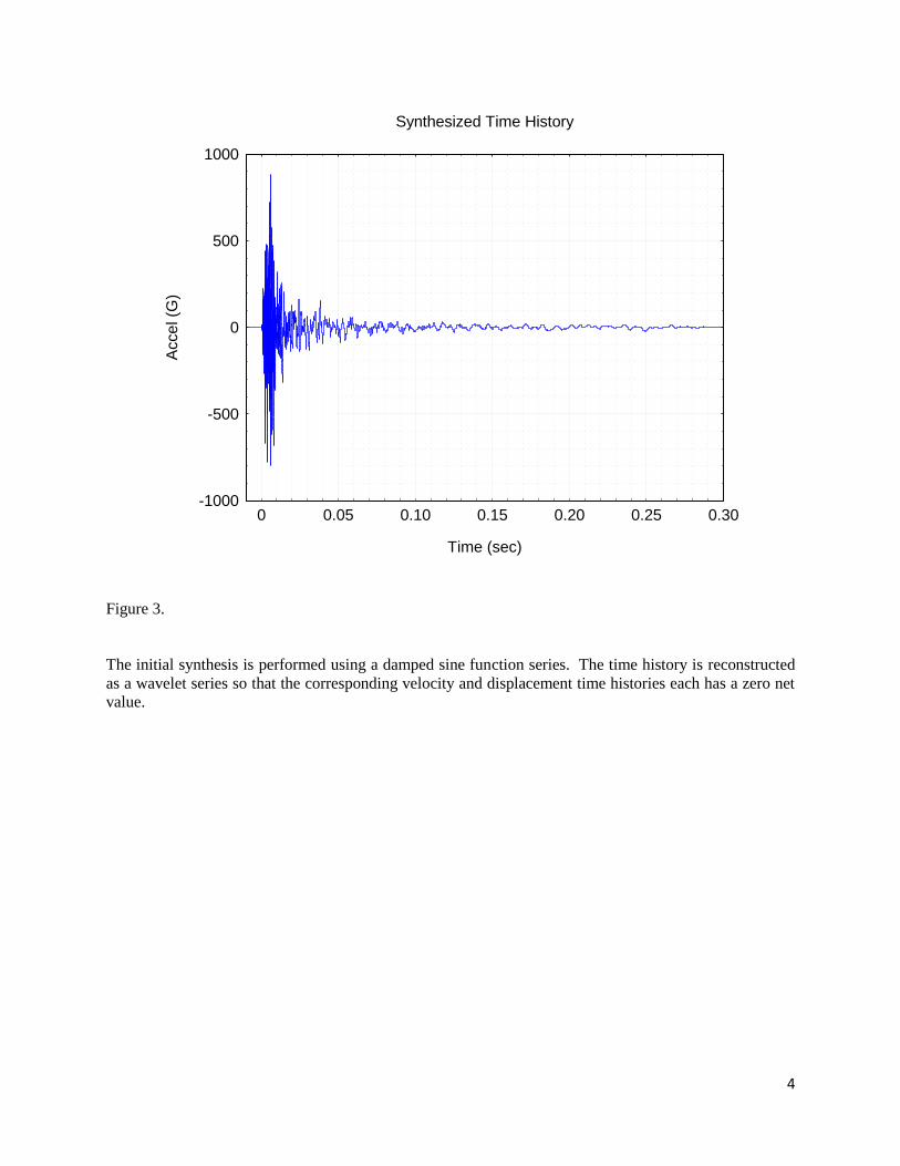
Figure 3.

The initial synthesis is performed using a damped sine function series. The time history is reconstructed

as a wavelet series so that the corresponding velocity and displacement time histories each has a zero net

value.

-1000

-500

0

500

1000

0 0.05 0.10 0.15 0.20 0.25 0.30

Time (sec)

Acce

l (G

)

Synthesized Time History

5

Sample Responses

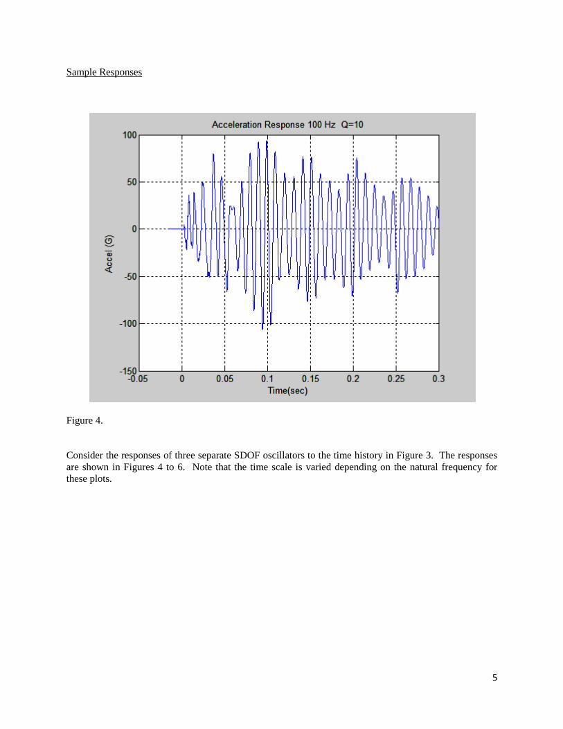
Figure 4.

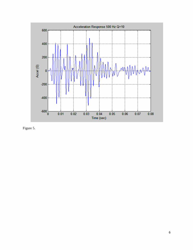
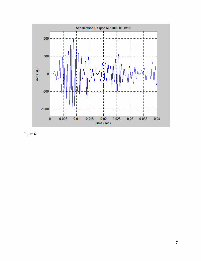
Consider the responses of three separate SDOF oscillators to the time history in Figure 3. The responses

are shown in Figures 4 to 6. Note that the time scale is varied depending on the natural frequency for

these plots.

6

Figure 5.

7

Figure 6.

8

Wavelet Model

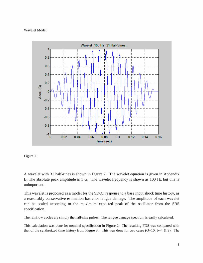
Figure 7.

A wavelet with 31 half-sines is shown in Figure 7. The wavelet equation is given in Appendix

B. The absolute peak amplitude is 1 G. The wavelet frequency is shown as 100 Hz but this is

unimportant.

This wavelet is proposed as a model for the SDOF response to a base input shock time history, as

a reasonably conservative estimation basis for fatigue damage. The amplitude of each wavelet

can be scaled according to the maximum expected peak of the oscillator from the SRS

specification.

The rainflow cycles are simply the half-sine pulses. The fatigue damage spectrum is easily calculated.

This calculation was done for nominal specification in Figure 2. The resulting FDS was compared with

that of the synthesized time history from Figure 3. This was done for two cases (Q=10, b=4 & 9). The

9

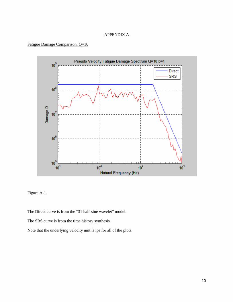
resulting plots are shown in Appendix A. The plots are given as pseudo velocity spectra. Note that

pseudo velocity tends to require fewer decades than either absolute acceleration or relative displacement.

The comparison shows that the “31 half-sine wavelet” model provides a conservative estimate of fatigue

for the two cases.

Additional Q Cases

The wavelet model has thus far assumed that the SDOF system’s Q value is the same as the SRS

specification. The wavelet scale factor for each frequency can thus be taken directly from the SRS curve.

A method for calculating the fatigue damage for cases where the Q factors differ is given in Appendix C.

Conclusion

The “31 half-sine wavelet” model appears to be good method for calculating a reasonably conservative

FDS from an SRS. Further verification is desirable.

References

1. T. Irvine, Using a Random Vibration Test to Cover a Shock Requirement, Revision D,

Vibrationdata, 2014.

2. T. Irvine, The Impulse Response Function for Base Excitation, Vibrationdata, 2012.

10

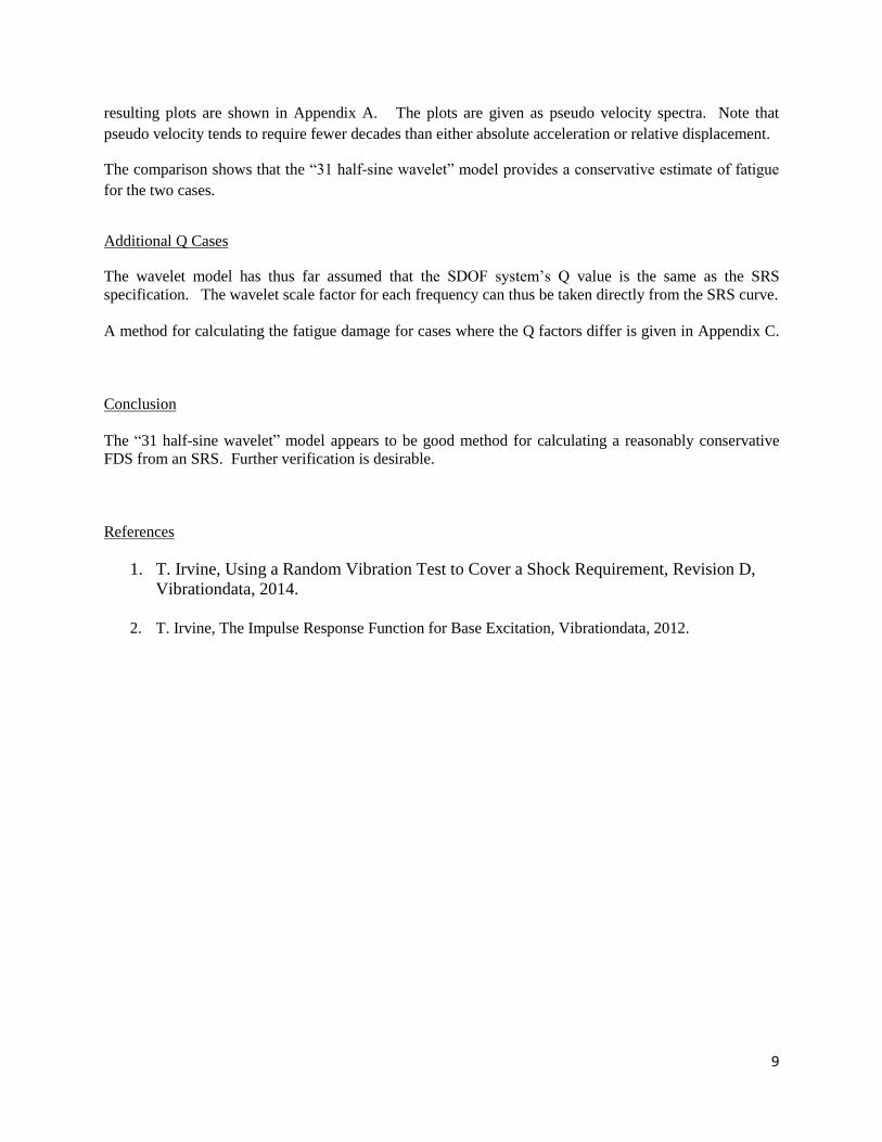
APPENDIX A

Fatigue Damage Comparison, Q=10

Figure A-1.

The Direct curve is from the “31 half-sine wavelet” model.

The SRS curve is from the time history synthesis.

Note that the underlying velocity unit is ips for all of the plots.

11

Figure A-2

12

APPENDIX B

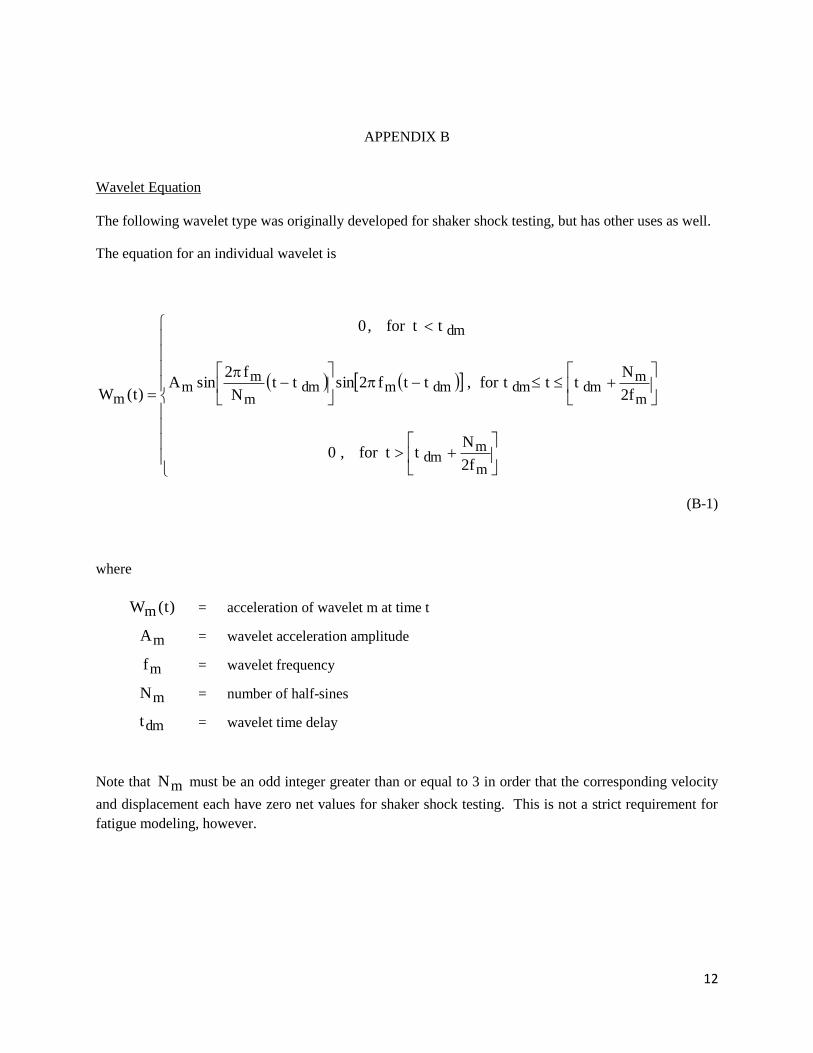
Wavelet Equation

The following wavelet type was originally developed for shaker shock testing, but has other uses as well.

The equation for an individual wavelet is

m

mdm

m

mdmdmdmmdm

m

mm

dm

m

f2

Nttfor,0

f2

Ntttfor,ttf2sintt

N

f2sinA

ttfor,0

)t(W

(B-1)

where

)t(Wm = acceleration of wavelet m at time t

mA = wavelet acceleration amplitude

mf = wavelet frequency

mN = number of half-sines

dmt = wavelet time delay

Note that mN must be an odd integer greater than or equal to 3 in order that the corresponding velocity

and displacement each have zero net values for shaker shock testing. This is not a strict requirement for

fatigue modeling, however.

13

APPENDIX C

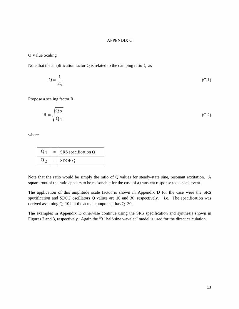
Q Value Scaling

Note that the amplification factor Q is related to the damping ratio as

2

1Q (C-1)

Propose a scaling factor R.

1

2

Q

QR (C-2)

where

1Q = SRS specification Q

2Q = SDOF Q

Note that the ratio would be simply the ratio of Q values for steady-state sine, resonant excitation. A

square root of the ratio appears to be reasonable for the case of a transient response to a shock event.

The application of this amplitude scale factor is shown in Appendix D for the case were the SRS

specification and SDOF oscillators Q values are 10 and 30, respectively. i.e. The specification was

derived assuming Q=10 but the actual component has Q=30.

The examples in Appendix D otherwise continue using the SRS specification and synthesis shown in

Figures 2 and 3, respectively. Again the “31 half-sine wavelet” model is used for the direct calculation.

14

APPENDIX D

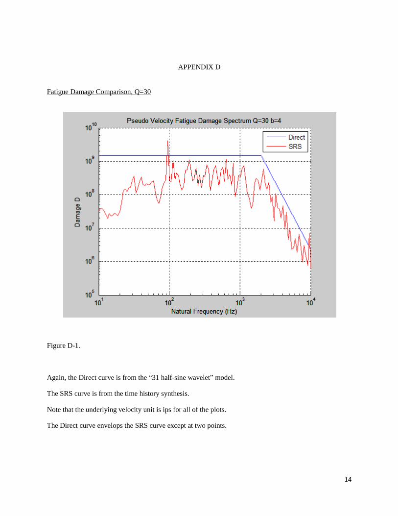
Fatigue Damage Comparison, Q=30

Figure D-1.

Again, the Direct curve is from the “31 half-sine wavelet” model.

The SRS curve is from the time history synthesis.

Note that the underlying velocity unit is ips for all of the plots.

The Direct curve envelops the SRS curve except at two points.

15

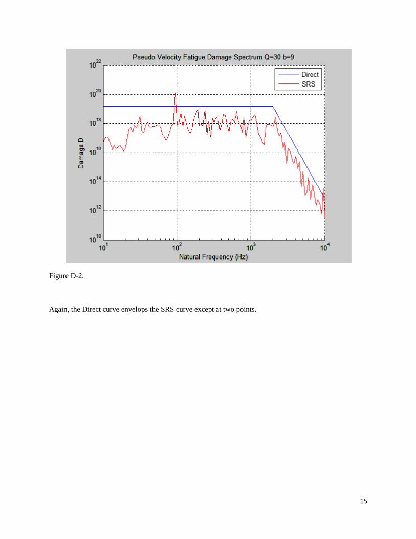
Figure D-2.

Again, the Direct curve envelops the SRS curve except at two points.