Embed Size (px)
Citation preview

Directorate General FOR
DIRECTORATE GENERAL FOR INTERNAL POLICIES
POLICY DEPARTMENT B: STRUCTURAL AND COHESION POLICIES
AGRICULTURE AND RURAL DEVELOPMENT
COMPARATIVE ANALYSIS OF AGRICULTURAL SUPPORT WITHIN
THE MAJOR AGRICULTURAL TRADING NATIONS
STUDY
This document was requested by the European Parliament's Committee on Agriculture and Rural Development. AUTHORS Mr Jean-Pierre BUTAULT, Mr Jean-Christophe BUREAU, Mr Heinz-Peter WITZKE, Mr Thomas HECKELEI1 RESPONSIBLE ADMINISTRATOR Mr Albert MASSOT Policy Department Structural and Cohesion Policies European Parliament B-1047 Brussels E-mail: [email protected] EDITORIAL ASSISTANCE Mrs Catherine MORVAN LINGUISTIC VERSIONS Original: EN. Translations: DE, FR. Exective summary in all languages. ABOUT THE EDITOR To contact the Policy Department or to subscribe to its monthly newsletter please write to: [email protected] Manuscript completed in March 2012. Brussels, © European Parliament, 2012. This document is available on the Internet at: http://www.europarl.europa.eu/studies DISCLAIMER The opinions expressed in this document are the sole responsibility of the author and do not necessarily represent the official position of the European Parliament. Reproduction and translation for non-commercial purposes are authorized, provided the source is acknowledged and the publisher is given prior notice and sent a copy.
1 The authors thank Lars BRINK for his comments.
DIRECTORATE GENERAL FOR INTERNAL POLICIES
POLICY DEPARTMENT B: STRUCTURAL AND COHESION POLICIES
AGRICULTURE AND RURAL DEVELOPMENT
COMPARATIVE ANALYSIS OF AGRICULTURAL SUPPORT WITHIN
THE MAJOR AGRICULTURAL TRADING NATIONS
STUDY
Abstract: Indicators of real support make it possible to compare policies across countries. EU farmers are more supported than their US colleagues, but EU support generates little distortion on world markets. US and Canada adjust support to protect farmers from adverse situations. Like the growing levels of support in Russia and China, these policies generate market distortions. Swiss support is directed towards the provision of public goods. In some countries such as Brazil, agricultural support targets innovation while most EU support has a focus on farm income.
IP/B/AGRI/IC/2011-068 May 2012 PE 474.544 EN

Policy Department B: Structural and Cohesion Policies _________________________________________________________________________________
PE 474.544 3
CONTENTS
LIST OF ABBREVIATIONS 5
LIST OF TABLES 7
LIST OF FIGURES 7
EXECUTIVE SUMMARY 13
1. INTRODUCTION 25
1.1. Measuring agricultural support 25
1.2. The types of policy instruments used to support agriculture 26
1.3. The indicators most commonly used 29
1.4. Political issues associated with these systems of comparison 33
2. METHODOLOGY FOR COMPARISON 35
2.1. Identifying the goals of agricultural support 35
2.2. What is asked from a measurement of agricultural support? 37
2.3. The pros and cons of the main measurements of farm support 38
2.4. How do measurements differ? The case of the EU 46
2.5. The methodology adopted in the study 48
2.6. Conclusion: the methodology adopted 59
3. RESULTS OF THE COMPARISON 61
3.1. A comparison of agricultural support in OECD countries 61
3.2. A comparison with selected non-OECD countries 74
4. AGRICULTURAL SUPPORT IN THE EU 83
4.1. Changes in the structure of agricultural support in the EU 83
4.2. EU agricultural support: A picture using the EU budget 86
4.3. EU agricultural support: A picture using data on farm subsidies 89
4.4. EU agricultural support: A picture based on the OECD information 91
4.5. EU agricultural support: A picture based on WTO notifications 97
4.6. The issue of the EU biofuel programme 99
4.7. Conclusion 100
5. COMPARING EU AGRICULTURAL SUPPORT WITH SELECTED OTHER COUNTRIES 103
5.1. Agricultural support in the United States 103
5.2. Agricultural support in Canada 113
5.3. Agricultural support in Switzerland 119
5.4. Conclusion 126
Comparative analysis of agricultural support within the major agricultural trading nations ___________________________________________________________________________________________
PE 474.544 4
6. EU SUPPORT IN THE FUTURE 127
6.1. The future CAP 127
6.2. Alternative directions for the post 2013 CAP 132
7. CONCLUSION 139
BIBLIOGRAPHY 141
ANNEXES 149
Annex 1. The OECD indicators 149
Annex 2. PSE categories and sub categories 151
Annex 3. PSE labels 153
Annex 4. The US layers of payments to farmers 154
Policy Department B: Structural and Cohesion Policies _________________________________________________________________________________
PE 474.544 5
LIST OF ABBREVIATIONS
ACRE Average Crop Revenue Election (US Program) ACT All Commodity Transfers AES Agri-Environmental Scheme AMS Aggregate Measure of Support AWU Annual Worker Unit CAP Common Agricultural Policy CCP Countercyclical Payments (USA) CRP Conservation Reserve Program CSE Consumer Support Estimate CV Compensating Variation DRC Domestic Resources Cost EAFRD European Agricultural Fund for Rural Development EAGF European Agricultural Guarantee Fund EIP European Innovation Partnership ERDF European Regional Development Fund ERS Economic Research Service (USDA) EU European Union EV Equivalent Variation EQIP Environmental Quality Incentives Program (USA) FADN Farm Accounting Data Network FAO Food and Agriculture Organisation FCEA Food, Conservation and Energy Act FEAGA See EAGF (French acronym) FEADER See EAFRD (French acronym) GAEC Good Agricultural and Environmental Conditions GCT Group Commodity Transfer GDP Gross Domestic Product GNI Gross National Income GSSE General Services Support Estimate HNV High Natural Value LDP Loan Deficiency Payment (USA) LFA Less Favoured Area MFF Multiannual Financial Framework MFN Most Favoured Nation MPS Market Price Support MTRI Mercantilistic Trade Restrictiveness Index NAC Nominal Assistance Coefficient NPC Nominal Protection Coefficient NGO Non Governmental Organisation NMS New Member States OECD Organisation for Economic Co-operation and Development OCT Other Commodity Transfer OTDS Overall Trade Distorting Support PER Prestations Ecologiques Requises (Switzerland) PPP Purchasing Power Parity PSE Producer Support Estimate (formerly Producer Subsidy Equivalent) RICA See FADN
Comparative analysis of agricultural support within the major agricultural trading nations ___________________________________________________________________________________________
PE 474.544 6
R&D Research and Development SAPS Single Area Payment Scheme SCT Single Commodity Transfer SFP Single Farm Payment SPS Single Payment Scheme SMR Statutory Management Requirement TRI Trade Restrictiveness Index TSE Total Support Estimate UK United Kingdom UAA Utilised Agricultural Area URAA Uruguay Round Agreement on Agriculture US United States (of America) USDA United States Department of Agriculture VAT Value Added Tax WTO World Trade Organization
Policy Department B: Structural and Cohesion Policies _________________________________________________________________________________
PE 474.544 7
LIST OF TABLES
Table 1. Indicative impact of support instruments on transfer efficiency and trade distortions 37 Table 2. Agricultural Support in the EU using OECD sources, comparison with the United States, 2007 47 Table 3. Agricultural Support in the EU using WTO sources, comparison with the United States, 2007/2998. 48 Table 4. Exchange rate, PPP and inflation rate in OECD countries 55 Table 5. Exchange rate, PPP and inflation rate in selected OECD and emerging economies 55 Table 6. Changes in the composition of real support over time 67 Table 7. PSE in nominal value, real value and percentage of farm receipts, 2010 79 Table 8. TSE in nominal value, in real value (2005 PPP) and as a percentage of farm receipts and GDP, 2010 80 Table 9. Main forms of support for selected non-OECD countries 81 Table 10. Main direct payments in the EU, 2010 93 Table 11. Major forms of support in US agriculture, 2009 and 2010 111 Table 12. Major forms of agricultural support, Canada 117 Table 13. Swiss payments, OECD and WTO classification 125 Table 14. Main support instruments, Switzerland, 2010 126

Comparative analysis of agricultural support within the major agricultural trading nations ___________________________________________________________________________________________
PE 474.544 8
Policy Department B: Structural and Cohesion Policies _________________________________________________________________________________
PE 474.544 9
LIST OF FIGURES Figure 1. Agricultural support in the EU according to various approaches 47 Figure 2. Nominal exchange rate and real (PPP) exchange rate 56 Figure 3. Computation of an OECD wide PSE expressed in various currencies 56 Figure 4. Sensitivity of PPP based aggregation to inflation in a particular country 57 Figure 5. Percentage PSE for the OECD as a whole and the choice of an exchange rate 57 Figure 6. Comparison of changes in the OECD PSE expressed in real terms and in percentage 58 Figure 7. Aggregate PSE for emerging countries, comparison of exchange rates aggregators 58 Figure 8. Border and domestic price, producer NPC, OECD countries 62 Figure 9. Variations over time of border prices, selected countries 63 Figure 10. Variations of border prices across commodities, OECD average 63 Figure 11. Evolution of price support, selected countries 64 Figure 12. Changes in price support, for selected countries 2010 relative to 1986 (price component and Single Commodity Transfer component) 65 Figure 13. Changes in real support and composition over time, OECD as a whole 66 Figure 14. Changes in payments over time, OECD as a whole, in real values 66 Figure 15. Change in the volume of agricultural production, selected OECD countries and emerging countries 68 Figure 16. Changes in the real value of production, selected OECD countries, 1986-2010 69 Figure 17. Changes in the real value of agricultural production, selected emerging countries, 1995-2010. 69 Figure 18. Changes in the real value of selected products, selected emerging countries, 1995-2010 70 Figure 19. Changes over time and composition of real support (in 2008-2010), selected countries 71 Figure 20. Percentage PSE 2008-2010 for selected OECD countries 72 Figure 21. Changes in farm receipts between 1986 and 2010, selected OECD countries 72 Figure 22. Real total support (TSE), changes in selected countries 1986-2010 73
Comparative analysis of agricultural support within the major agricultural trading nations ___________________________________________________________________________________________
PE 474.544 10
Figure 23. Total support as a percentage of GDP 74 Figure 24. Changes in the percentage PSE, selected emerging countries, 1995-2010 76 Figure 25. Changes in real agricultural output and share of public support, 1995-2010 76 Figure 26. Changes in real price support, Brazil, 1995-2010 77 Figure 27. Changes in real price support, China, 1995-2010 77 Figure 28. Price support as measured by the Nominal Protection Coefficient 78 Figure 29. Product specific support in selected emerging countries, 2010 78 Figure 30. Non commodity specific support as a percentage of agricultural gross receipts 79 Figure 31. Change in Chinese real PSE, a comparison with OECD as a whole (1995-2010). 82 Figure 32. Changes in the product specific support as measured by the OECD and the WTO (AMS specific) 1995 -2007 85 Figure 33. Changes in the total support as measured by the OECD (TSE) and the WTO (Green, Blue, Amber and de minimis) 1995 -2007 85 Figure 34. Agricultural expenditures, annual, changes in constant euro, EU, 1990-2010. 87 Figure 35. Agricultural budget, composition, in constant euro, EU, 1990-2010. 87 Figure 36. Product specific budgetary expenditure, EU, 1990-2010 88 Figure 37. Farm subsidies in EU economic accounts as a percent of net income, 1995-2010 90 Figure 38. Farm subsidies in FADN (EU 15), 1995-2008 91 Figure 39. Domestic prices and world prices, EU, 1986-2010 92 Figure 40. Changes in commodity specific support over time, EU, 1086-2010 92 Figure 41. Changes in the types of payments to producers over time, EU 94 Figure 42. Farm receipts and share of support, constant terms for EU19 95 Figure 43. Evolution of the support granted to EU agriculture through general services 96 Figure 44. Evolution of total support estimate, EU 96 Figure 45. Composition of EU total transfers (TSE) 97 Figure 46. Support under the various WTO categories, EU, 1995-2008 98 Figure 47. Composition of Amber Box support, EU, 1995-2008 99
Policy Department B: Structural and Cohesion Policies _________________________________________________________________________________
PE 474.544 11
Figure 48. Evolution of price support over time in the US, 1986-2010 104 Figure 49. Evolution of US NPC, selected commodities, 1986-2010 105 Figure 50. Expenditure under the various schemes that compensate farmers for losses 106 Figure 51. Changes in the composition of US support to agriculture, OECD classification, 1986-2010 108 Figure 52. Changes in the composition of US support to agriculture, 1986-2010 109 Figure 53. Farm receipts and the level of the US PSE, 1986-2010 109 Figure 54. Changes in the US net farm income and total payments, 1986-2010 110 Figure 55. The general services component of the TSE, US, 1986-2010 110 Figure 56. Distorting support and maximum WTO ceiling, US, 1995-2009 112 Figure 57. Evolution of price support over time in Canada, 1986-2010 114 Figure 58. PSE and percentage PSE in Canada, 1986-2010 114 Figure 59. Composition of product specific support, Canada, 1986-2010 115 Figure 60. Composition of non commodity specific support, Canada, 1986-2010 115 Figure 61. Changes in total support according to WTO notifications, Canada 1995-2007 117 Figure 62. Support and farm receipts, Canada, 1986-2010 118 Figure 63. Evolution of price support over time in Switzerland, 1986-2010 120 Figure 64. Coupled support, selected outputs, Switzerland, 1986-2010 120 Figure 65. Evolution of PSE, Switzerland, 1986-2010 122 Figure 66. Agricultural support as a share of farm receipts, Switzerland, 1986-2010 123 Figure 67. Agricultural income and support, Switzerland, 1986-2010 123 Figure 68. Changes in total support according to WTO notifications, Switzerland 1995-2007 124

Comparative analysis of agricultural support within the major agricultural trading nations ___________________________________________________________________________________________
PE 474.544 12
Policy Department B: Structural and Cohesion Policies _________________________________________________________________________________
PE 474.544 13
EXECUTIVE SUMMARY
Issues with agricultural support Countries support their agriculture at many different levels, for different purposes and using a variety of instruments. Support to agriculture can take the form of budgetary transfers. These can be measured either through budgetary expenditures (national accounts) or through subsidies received by farmers (microeconomic sources). There are, however, many other non-budgetary ways to support producers. Governments support prices using a variety of instruments, such as border protection, production quotas or public purchases. The support resulting from these instruments cannot be neglected. Agricultural support can also be more indirect, through subsidies that cover some of the farmers' costs (e.g., tax exemptions, subsidised interest rates), or through government support of general services (e.g., research, extension, health insurance). Policies can also generate additional demand for agricultural products and drive up prices. This is the case of food aid policies or policies that promote biofuels. Estimating the actual impact on farmers is difficult, but the level of public expenditure can be considerable (e.g., the budget of the US "food stamp" programme). Despite the difficulty in measuring transfers by price support and indirect aid, the focus on budgetary transfers alone does not lead to meaningful comparisons between countries, between products (some are supported by tariffs or guaranteed prices, and others are not), or even within a country. For example, the EU has gradually replaced support paid by the consumer with support paid by the taxpayer. While this led to a larger agricultural budget, it would be misleading to take this as an increase in overall support for agriculture. Data limitations A considerable amount of resources is necessary to make information from budget or microeconomic sources comparable across countries. The accounting framework, what is included in the agricultural sector and the economic concepts underlying the accounting codes are often very different. The OECD Secretariat (Organisation for Economic Cooperation and Development) has compiled a dataset for 33 Member states and selected emerging countries. Figures are subject to an intensive check by the national governments and, overall the OECD dataset is a reliable and comprehensive data source. Another source is the notifications on domestic support that World Trade Organization (WTO) member countries submit to the Secretariat. These data are seldom up to date and are not particularly reliable, given that similar measures are sometimes classified into different categories across countries. Nevertheless, the WTO data, and in particular its classification of support are useful for certain questions. Other data sources are more partial and less reliable.
Comparative analysis of agricultural support within the major agricultural trading nations ___________________________________________________________________________________________
PE 474.544 14
The measurement of price support Price support may take the form of a direct subsidy per unit of production, or an increase in market price caused by government intervention. The most appropriate methods to measure such transfers involve the use of global models to compare the actual situation of producers with the counterfactual where this support would not exist. In such a case one can define theoretically sound indicators (e.g., variations in consumer surplus, equivalent or compensating variations). Alternatively, if one looks at the effects on trade, indicators of trade restrictiveness may be used. A limitation arises when generating the counterfactual situation with a model: the result is dependent on parameters and assumptions that limit the practical scope of this theoretically satisfactory framework. Moreover, in the work of the international organizations mandated to measure support, comparisons over time and between countries must use simple indicators, in order to avoid contradictions between results obtained under a variety of models. In practice, two approaches are widely used. The main indicator of support used by the WTO, the Aggregate Measurement of Support (AMS) has serious limitations. The price support element uses the difference between administered prices and world reference prices at a fixed base period. It may be positive in the absence of actual support if a country maintains an administrative support price higher than the fixed reference price. The market price support for wheat in the EU, for example, has been positive even at times when the intervention price was half of the world price. This shows that the measure has little economic meaning it is also possible to remove support elements of several billion dollars by implementing relatively minor policy changes that appear in the notifications simply as a change in practice (e.g., milk in the US, fruit and vegetables in the EU). The OECD approach is more related to market realities. Price support is measured as the difference between current domestic prices and current border prices, regardless of the origin of this difference, provided that a policy is being applied. This indicator has been subject to refinement but also to recurrent criticism for 25 years. The use of a world price, which depends itself on support policies, is arguably a questionable reference. This criticism merely shows that OECD indicators such as the Producer Support Estimate (PSE) should be interpreted only as calculations in a static framework where the border price is an objective reality. The OECD PSE is also sensitive to the currency used for aggregation; the choice of the statistical series for some reference prices is questionable; the classification of different supports policies cannot be interpreted in terms of the distorting nature of the policy; and the need to distinguish a large variety of payments and indicators to reflect the nature of farm support in each country have made it difficult to communicate the results effectively. In spite of these caveats the PSE methodology has many attractive features. The methodology used in the report In the report, many indicators rely on the OECD dataset, even though budgets and WTO notifications are also used in particular sections of the report. Some of the OECD indicators, i.e., PSE, Total Support Estimates (TSE) and Nominal Protection Coefficient (NPC) are also used, but several changes were made to the methodology. First, in order to account for the effects of changes in agricultural policy and the effects of exchange rates and inflation differentials between countries, support indicators are calculated in real terms. This requires the construction of a conversion rate for a base year (here 2005) and the use of a spatial price index, a Purchasing Power Parity (PPP) measure. Both this base period PPP and a time series for deflators are used to aggregate the real
Policy Department B: Structural and Cohesion Policies _________________________________________________________________________________
PE 474.544 15
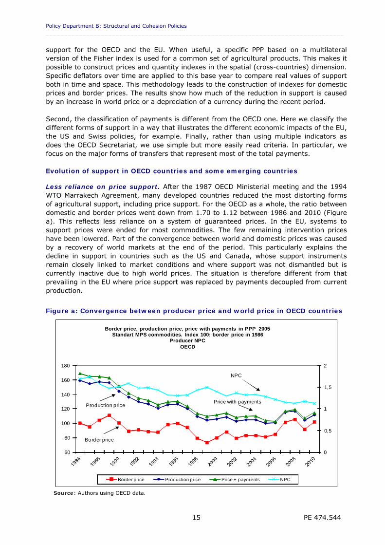
support for the OECD and the EU. When useful, a specific PPP based on a multilateral version of the Fisher index is used for a common set of agricultural products. This makes it possible to construct prices and quantity indexes in the spatial (cross-countries) dimension. Specific deflators over time are applied to this base year to compare real values of support both in time and space. This methodology leads to the construction of indexes for domestic prices and border prices. The results show how much of the reduction in support is caused by an increase in world price or a depreciation of a currency during the recent period. Second, the classification of payments is different from the OECD one. Here we classify the different forms of support in a way that illustrates the different economic impacts of the EU, the US and Swiss policies, for example. Finally, rather than using multiple indicators as does the OECD Secretariat, we use simple but more easily read criteria. In particular, we focus on the major forms of transfers that represent most of the total payments. Evolution of support in OECD countries and some emerging countries Less reliance on price support. After the 1987 OECD Ministerial meeting and the 1994 WTO Marrakech Agreement, many developed countries reduced the most distorting forms of agricultural support, including price support. For the OECD as a whole, the ratio between domestic and border prices went down from 1.70 to 1.12 between 1986 and 2010 (Figure a). This reflects less reliance on a system of guaranteed prices. In the EU, systems to support prices were ended for most commodities. The few remaining intervention prices have been lowered. Part of the convergence between world and domestic prices was caused by a recovery of world markets at the end of the period. This particularly explains the decline in support in countries such as the US and Canada, whose support instruments remain closely linked to market conditions and where support was not dismantled but is currently inactive due to high world prices. The situation is therefore different from that prevailing in the EU where price support was replaced by payments decoupled from current production.
Figure a: Convergence between producer price and world price in OECD countries
0
0,5
1
1,5
2
60
80
100
120
140
160
180
Border price, production price, price with payments in PPP_2005Standart MPS commodities. Index 100: border price in 1986
Producer NPCOECD
Border price Production price Price + payments NPC
Border price
Production pricePrice with payments
NPC
Source: Authors using OECD data.
Comparative analysis of agricultural support within the major agricultural trading nations ___________________________________________________________________________________________
PE 474.544 16
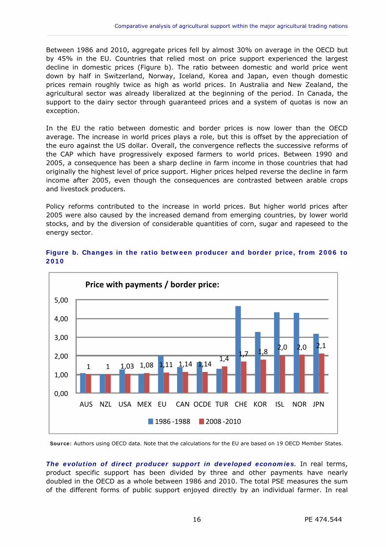
Between 1986 and 2010, aggregate prices fell by almost 30% on average in the OECD but by 45% in the EU. Countries that relied most on price support experienced the largest decline in domestic prices (Figure b). The ratio between domestic and world price went down by half in Switzerland, Norway, Iceland, Korea and Japan, even though domestic prices remain roughly twice as high as world prices. In Australia and New Zealand, the agricultural sector was already liberalized at the beginning of the period. In Canada, the support to the dairy sector through guaranteed prices and a system of quotas is now an exception. In the EU the ratio between domestic and border prices is now lower than the OECD average. The increase in world prices plays a role, but this is offset by the appreciation of the euro against the US dollar. Overall, the convergence reflects the successive reforms of the CAP which have progressively exposed farmers to world prices. Between 1990 and 2005, a consequence has been a sharp decline in farm income in those countries that had originally the highest level of price support. Higher prices helped reverse the decline in farm income after 2005, even though the consequences are contrasted between arable crops and livestock producers. Policy reforms contributed to the increase in world prices. But higher world prices after 2005 were also caused by the increased demand from emerging countries, by lower world stocks, and by the diversion of considerable quantities of corn, sugar and rapeseed to the energy sector.
Figure b. Changes in the ratio between producer and border price, from 2006 to 2010
Source: Authors using OECD data. Note that the calculations for the EU are based on 19 OECD Member States.
The evolution of direct producer support in developed economies. In real terms, product specific support has been divided by three and other payments have nearly doubled in the OECD as a whole between 1986 and 2010. The total PSE measures the sum of the different forms of public support enjoyed directly by an individual farmer. In real
1 1 1,03 1,08 1,11 1,14 1,14 1,4
1,7 1,8 2,0 2,0 2,1
0,00
1,00
2,00
3,00
4,00
5,00
AUS NZL USA MEX EU CAN OCDE TUR CHE KOR ISL NOR JPN
Price with payments / border price:
1986 ‐ 1988 2008 ‐ 2010
Policy Department B: Structural and Cohesion Policies _________________________________________________________________________________
PE 474.544 17
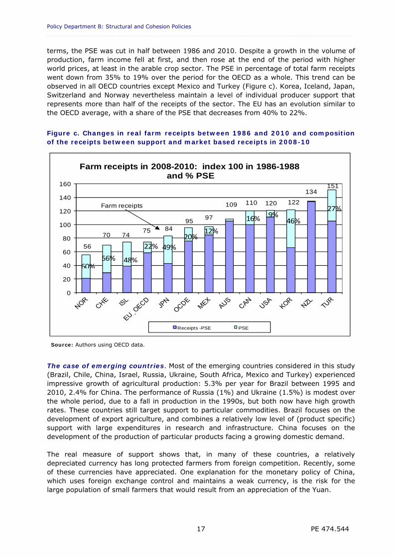
terms, the PSE was cut in half between 1986 and 2010. Despite a growth in the volume of production, farm income fell at first, and then rose at the end of the period with higher world prices, at least in the arable crop sector. The PSE in percentage of total farm receipts went down from 35% to 19% over the period for the OECD as a whole. This trend can be observed in all OECD countries except Mexico and Turkey (Figure c). Korea, Iceland, Japan, Switzerland and Norway nevertheless maintain a level of individual producer support that represents more than half of the receipts of the sector. The EU has an evolution similar to the OECD average, with a share of the PSE that decreases from 40% to 22%.
Figure c. Changes in real farm receipts between 1986 and 2010 and composition of the receipts between support and market based receipts in 2008-10
0
20
40
60
80
100
120
140
160
Farm receipts in 2008-2010: index 100 in 1986-1988and % PSE
Receipts -PSE PSE
56
70 7475 84
9597
109 110 120 122
134151
Farm receipts
60%56% 48%
22% 49%
20%12%
16% 9%46%
27%
Source: Authors using OECD data.
The case of emerging countries. Most of the emerging countries considered in this study (Brazil, Chile, China, Israel, Russia, Ukraine, South Africa, Mexico and Turkey) experienced impressive growth of agricultural production: 5.3% per year for Brazil between 1995 and 2010, 2.4% for China. The performance of Russia (1%) and Ukraine (1.5%) is modest over the whole period, due to a fall in production in the 1990s, but both now have high growth rates. These countries still target support to particular commodities. Brazil focuses on the development of export agriculture, and combines a relatively low level of (product specific) support with large expenditures in research and infrastructure. China focuses on the development of the production of particular products facing a growing domestic demand. The real measure of support shows that, in many of these countries, a relatively depreciated currency has long protected farmers from foreign competition. Recently, some of these currencies have appreciated. One explanation for the monetary policy of China, which uses foreign exchange control and maintains a weak currency, is the risk for the large population of small farmers that would result from an appreciation of the Yuan.
Comparative analysis of agricultural support within the major agricultural trading nations ___________________________________________________________________________________________
PE 474.544 18
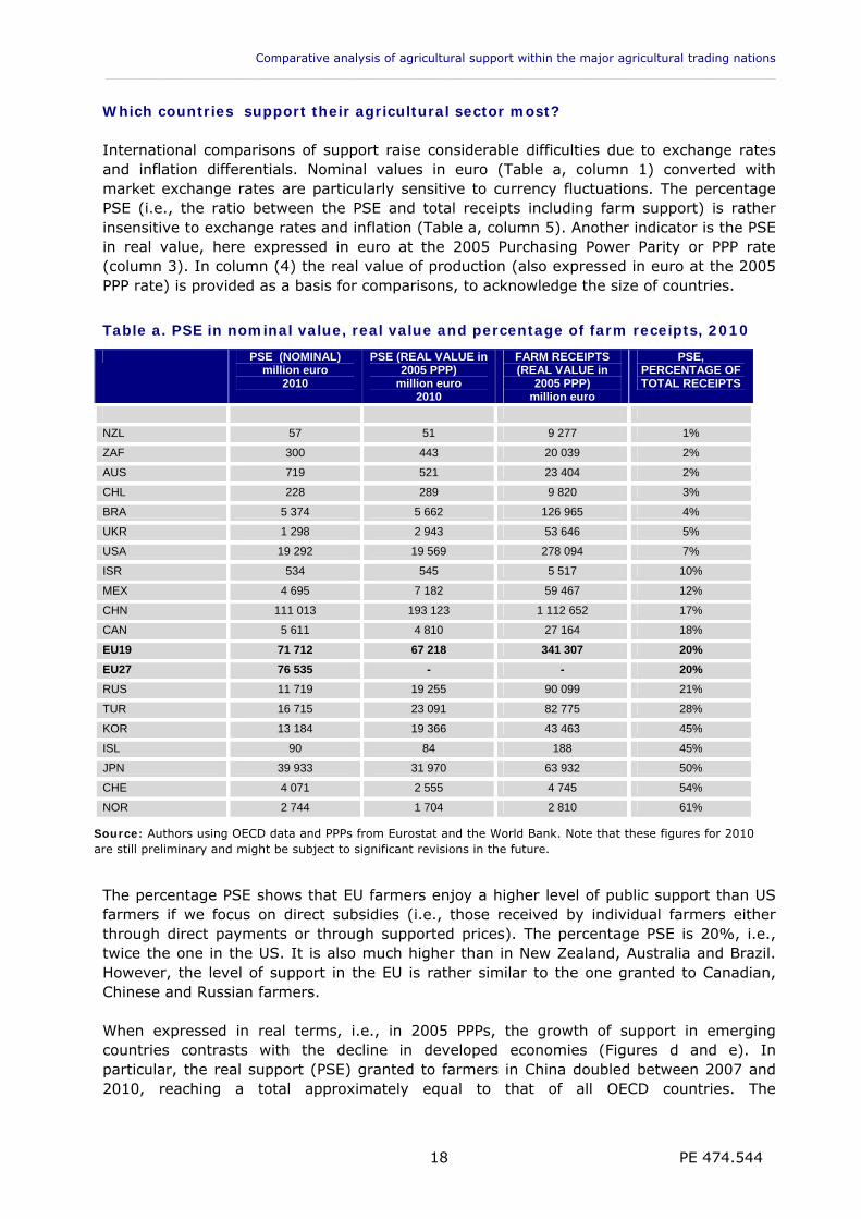
Which countries support their agricultural sector most? International comparisons of support raise considerable difficulties due to exchange rates and inflation differentials. Nominal values in euro (Table a, column 1) converted with market exchange rates are particularly sensitive to currency fluctuations. The percentage PSE (i.e., the ratio between the PSE and total receipts including farm support) is rather insensitive to exchange rates and inflation (Table a, column 5). Another indicator is the PSE in real value, here expressed in euro at the 2005 Purchasing Power Parity or PPP rate (column 3). In column (4) the real value of production (also expressed in euro at the 2005 PPP rate) is provided as a basis for comparisons, to acknowledge the size of countries.
Table a. PSE in nominal value, real value and percentage of farm receipts, 2010
PSE (NOMINAL) million euro
2010
PSE (REAL VALUE in 2005 PPP)
million euro 2010
FARM RECEIPTS (REAL VALUE in
2005 PPP) million euro
PSE, PERCENTAGE OF TOTAL RECEIPTS
NZL 57 51 9 277 1%
ZAF 300 443 20 039 2%
AUS 719 521 23 404 2%
CHL 228 289 9 820 3%
BRA 5 374 5 662 126 965 4%
UKR 1 298 2 943 53 646 5%
USA 19 292 19 569 278 094 7%
ISR 534 545 5 517 10%
MEX 4 695 7 182 59 467 12%
CHN 111 013 193 123 1 112 652 17%
CAN 5 611 4 810 27 164 18%
EU19 71 712 67 218 341 307 20%
EU27 76 535 - - 20%
RUS 11 719 19 255 90 099 21%
TUR 16 715 23 091 82 775 28%
KOR 13 184 19 366 43 463 45%
ISL 90 84 188 45%
JPN 39 933 31 970 63 932 50%
CHE 4 071 2 555 4 745 54%
NOR 2 744 1 704 2 810 61%
Source: Authors using OECD data and PPPs from Eurostat and the World Bank. Note that these figures for 2010 are still preliminary and might be subject to significant revisions in the future.
The percentage PSE shows that EU farmers enjoy a higher level of public support than US farmers if we focus on direct subsidies (i.e., those received by individual farmers either through direct payments or through supported prices). The percentage PSE is 20%, i.e., twice the one in the US. It is also much higher than in New Zealand, Australia and Brazil. However, the level of support in the EU is rather similar to the one granted to Canadian, Chinese and Russian farmers. When expressed in real terms, i.e., in 2005 PPPs, the growth of support in emerging countries contrasts with the decline in developed economies (Figures d and e). In particular, the real support (PSE) granted to farmers in China doubled between 2007 and 2010, reaching a total approximately equal to that of all OECD countries. The
Policy Department B: Structural and Cohesion Policies _________________________________________________________________________________
PE 474.544 19
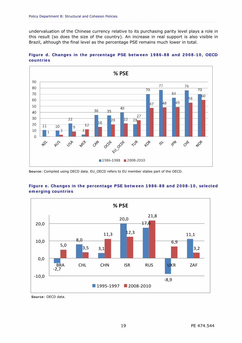
undervaluation of the Chinese currency relative to its purchasing parity level plays a role in this result (so does the size of the country). An increase in real support is also visible in Brazil, although the final level as the percentage PSE remains much lower in total.
Figure d. Changes in the percentage PSE between 1986-88 and 2008-10, OECD countries
Source: Compiled using OECD data. EU_OECD refers to EU member states part of the OECD.
Figure e. Changes in the percentage PSE between 1986-88 and 2008-10, selected emerging countries
‐2,7
8,0
3,1
20,017,6
‐8,9
11,1
5,03,5
11,3 12,3
21,8
6,9
3,2
‐10,0
0,0
10,0
20,0
BRA CHL CHN ISR RUS UKR ZAF
% PSE
1995‐1997 2008‐2010
Source: OECD data.
Comparative analysis of agricultural support within the major agricultural trading nations ___________________________________________________________________________________________
PE 474.544 20
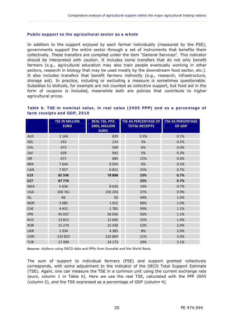
Public support to the agricultural sector as a whole In addition to the support enjoyed by each farmer individually (measured by the PSE), governments support the entire sector through a set of instruments that benefits them collectively. These transfers are compiled under the item "General Services". This indicator should be interpreted with caution. It includes some transfers that do not only benefit farmers (e.g., agricultural education may also train people eventually working in other sectors, research in biology that may be used mostly by the downstream food sector, etc.). It also includes transfers that benefit farmers indirectly (e.g., research, infrastructure, storage aid). In practice, including or excluding a measure is sometimes questionable. Subsidies to biofuels, for example are not counted as collective support, but food aid in the form of coupons is included, meanwhile both are policies that contribute to higher agricultural prices.
Table b. TSE in nominal value, in real value (2005 PPP) and as a percentage of farm receipts and GDP, 2010
TSE IN MILLION EURO
REAL TSE, PPA 2005, MILLION
EURO
TSE AS PERCENTAGE OF TOTAL RECEIPTS
TSE AS PERCENTAGE OF GDP
AUS 1 144 829 3.5% 0.1%
NZL 243 214 2% 0.2%
CHL 473 599 6% 0.3%
ZAF 639 942 5% 0.3%
ISR 671 684 12% 0.4%
BRA 7 644 8 054 6% 0.5%
CAN 7 957 6 822 25% 0.7%
E19 82 596 78 808 23% 0.7%
E27 87 770 ‐ 23% 0.7%
MEX 5 636 8 620 14% 0.7%
USA 100 761 102 203 37% 0.9%
ISL 66 92 49% 1.0%
NOR 3 085 1 915 68% 1.0%
CHE 4 431 2 782 59% 1.1%
JPN 45 037 36 056 56% 1.1%
RUS 13 813 22 695 25% 1.4%
KOR 15 270 22 430 52% 2.0%
UKR 1 934 4 385 8% 2.0%
CHN 133 823 232 804 21% 3.0%
TUR 17 499 24 173 29% 3.1%
Source: Authors using OECD data and PPPs from Eurostat and the World Bank.
The sum of support to individual farmers (PSE) and support granted collectively corresponds, with some adjustment to the indicator of the OECD Total Support Estimate (TSE). Again, one can measure the TSE in a common unit using the current exchange rate (euro, column 1 in Table b). Here we use the real TSE, calculated with the PPP 2005 (column 2), and the TSE expressed as a percentage of GDP (column 4).
Policy Department B: Structural and Cohesion Policies _________________________________________________________________________________
PE 474.544 21
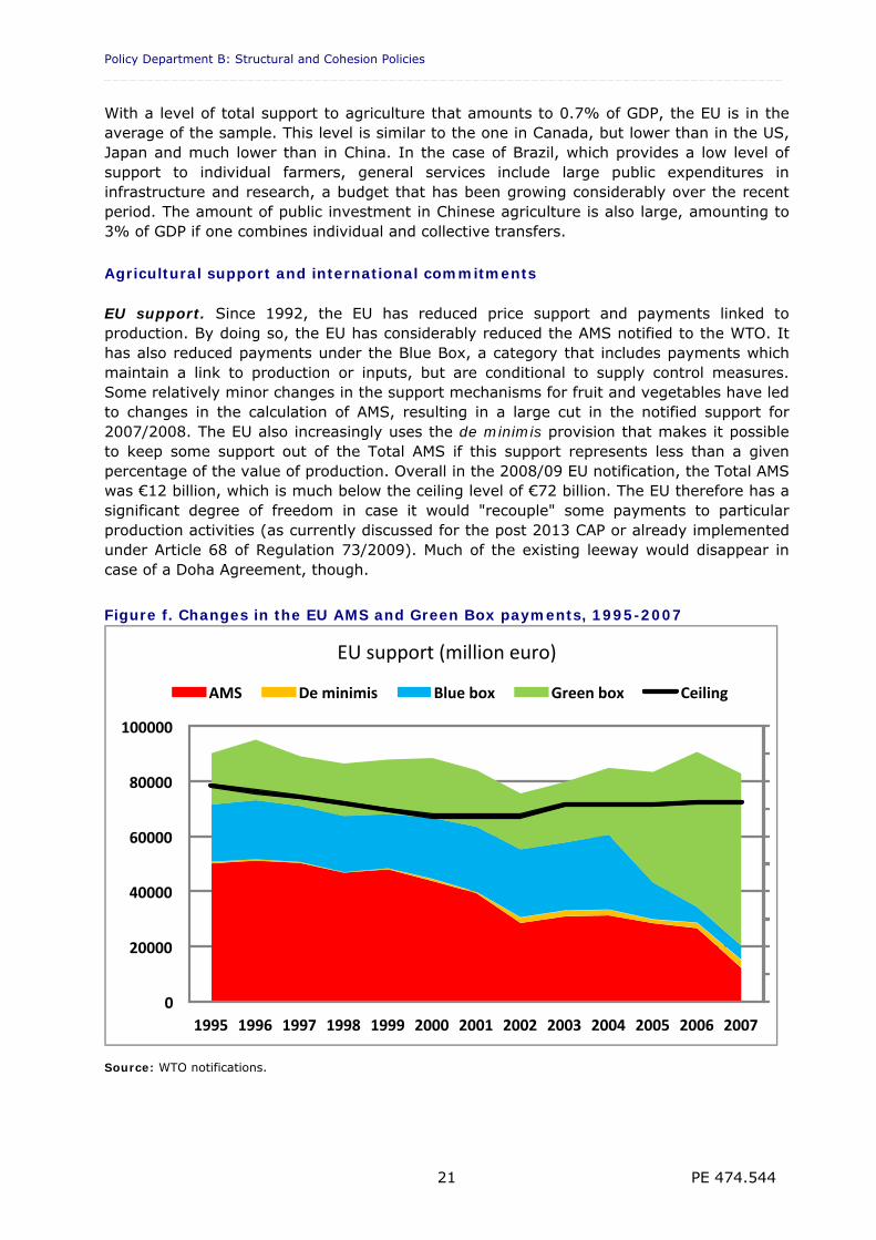
With a level of total support to agriculture that amounts to 0.7% of GDP, the EU is in the average of the sample. This level is similar to the one in Canada, but lower than in the US, Japan and much lower than in China. In the case of Brazil, which provides a low level of support to individual farmers, general services include large public expenditures in infrastructure and research, a budget that has been growing considerably over the recent period. The amount of public investment in Chinese agriculture is also large, amounting to 3% of GDP if one combines individual and collective transfers. Agricultural support and international commitments EU support. Since 1992, the EU has reduced price support and payments linked to production. By doing so, the EU has considerably reduced the AMS notified to the WTO. It has also reduced payments under the Blue Box, a category that includes payments which maintain a link to production or inputs, but are conditional to supply control measures. Some relatively minor changes in the support mechanisms for fruit and vegetables have led to changes in the calculation of AMS, resulting in a large cut in the notified support for 2007/2008. The EU also increasingly uses the de minimis provision that makes it possible to keep some support out of the Total AMS if this support represents less than a given percentage of the value of production. Overall in the 2008/09 EU notification, the Total AMS was €12 billion, which is much below the ceiling level of €72 billion. The EU therefore has a significant degree of freedom in case it would "recouple" some payments to particular production activities (as currently discussed for the post 2013 CAP or already implemented under Article 68 of Regulation 73/2009). Much of the existing leeway would disappear in case of a Doha Agreement, though.
Figure f. Changes in the EU AMS and Green Box payments, 1995-2007
Source: WTO notifications.
0
20000
40000
60000
80000
100000
1995 1996 1997 1998 1999 2000 2001 2002 2003 2004 2005 2006 2007
EU support (million euro)
AMS De minimis Blue box Green box Ceiling
Comparative analysis of agricultural support within the major agricultural trading nations ___________________________________________________________________________________________
PE 474.544 22
Meanwhile, the EU has increased its support in the Green Box category from €19 billion in 1995 to €63 billion in 2008/09, particularly as a result of decoupling (Figure f). The EU might therefore be above its Total AMS ceiling if the Green Box eligibility of these payments happened to be successfully challenged, an unlikely issue but one that was raised by Swinbank (2012) in the context of the European Commission proposal of October 2011. Other countries' AMS support is also below their WTO ceiling. For some particular year, the US Total AMS has stayed below the ceiling only because of an extensive use of the de minimis provision. Canada notifies support under certain insurance schemes in the Green Box, which has been questioned. Without recourse to the Green Box for this support, Canada would be much closer to its Total AMS ceiling. Many emerging countries have not yet notified their domestic support to the WTO for the most recent years. The most recent notifications still refer to 2003 in some cases. Calculations by consultants, involving particular interpretations of some countries’ policy regimes (e.g., India, Brazil, Thailand, Turkey), suggest that they could be in a situation where they exceed the limits of their WTO commitments (DTB Associates, 2011). A comparison of policy instruments Not all support instruments have the same effects. The economic literature suggests that price support and per unit of output payments are the instruments that have the strongest impacts on third-country producers. In terms of market distortions, such policies are followed by payments linked to inputs, by production quotas, and by payments based on historical references. Decoupled support has no or little impact on production. Payment for the cessation of production, for setting aside land or reducing the use of inputs may have a negative impact. In the EU, most of the support measured by the PSE no longer requires production and only 16% of it is based on actual production. The EU has radically transformed its agricultural policy over time. The impact of the EU support on world markets is now limited. In countries were the support measured by the PSE is very low, such as Australia and New Zealand, remaining payments tend to be granted on the basis of output or variable inputs. In the countries granting generous support to their agriculture, such as Norway, Switzerland, Japan and Korea, there has been a strong reduction of the most distorting forms of support over time. However, such distorting support still accounts for the bulk of the PSE (Japan, Korea) or for a large share of it (Switzerland, Norway). The case of emerging countries is very different from that of the EU. There has been rapid growth in agricultural support in China and Russia. In these countries, in 2010, support reaches levels comparable to those of the EU as a percentage of production and even more as a percentage of GDP (Table a and Table b). In addition, nearly two thirds of these supports (as measured by the PSE) are linked to current production and target particular commodities. There is no observable shift towards less decoupled support. China, in particular, increasingly supports a set of products it considers important for its food security. The examination of the composition of support also shows that subsidies or tax exemptions that lower energy prices for farmers are widespread and account for a significant share of the support.
Policy Department B: Structural and Cohesion Policies _________________________________________________________________________________
PE 474.544 23
The effects of biofuel support policies are neither recorded in the OECD nor in the WTO indicators.2 These policies now play an important role in the price determination of corn, sugar and oilseeds. Simulations on the EU using an econometric model suggest that they are equivalent to a policy of support for rapeseed production of over €1.5 billion in direct payments (Bureau et al. 2010). These results are nevertheless sensitive to assumptions about oil prices. Farm support provided by biofuels is particularly difficult to quantify with simple indicators. The Swiss, US and Canadian support: lessons for the CAP? In the EU, decoupled payments are the main form of support. These are followed by fuel subsidies, subsidies to investment, environmental payments and payments to less favoured areas. These transfers account for 70% of total support. In the US, the support linked to market prices is low at the end of the period. A striking difference with the EU is that the US policy relies heavily on a series of instruments to protect farm incomes against climatic hazards as well as unfavourable market conditions. The level of support (as measured by the percentage PSE) is lower than in the EU, but the payments are less decoupled and more market distorting. In Canada, support instruments also intend to protect farm incomes from fluctuations. Insurance systems play a greater role than in the EU, in particular. In Switzerland, all payments are conditional on strict environmental constraints. The Swiss policy also aims to maintain a certain level of production in the most difficult areas. The move towards decoupling was similar to the post 1992 CAP. The remaining support is higher than in the EU. The shift of support towards the provision of public goods has gone further than in the EU. The comparison of EU support with that in other countries can be useful in the current debates raised by the October 12, 2011 Commission proposal on the post 2013 CAP. One issue which is discussed is whether the EU support should be made more countercyclical, as is the case in the US. Adjusting the EU payments downwards when market conditions are good and upwards when farm incomes are low would help to smooth farm income variations and make the current system more acceptable to public opinion. However, this would have many unwanted effects: lack of compatibility with the structure and stability over time of the EU budget; lack of rationale of replacing farmer's own smoothing of receipts over time by administrative procedures; risk of blurring the signals of excess supply or excess demand to producers and thus potentially leading to market imbalances; making infeasible the conditionality of payments on good practices; and needing de facto to shift back to product-specific payments. The Commission's proposal also includes the development of risk management tools such as insurance. The US and Canadian experience suggests that the management costs and leakages in this form of support limit the transfer efficiency, i.e., the ratio of the amount benefiting farmers to the cost for taxpayers. A detailed analysis is beyond the scope of this report, but the cost efficiency of these measures compared to EU payments is uncertain. The Commission's proposal to "green" CAP support by conditioning 30% of the direct payments on a series of constraints including an "ecological focus" area has raised many criticisms. In this area, the Swiss experience goes beyond what the Commission proposes for the post 2013 CAP. Several assessments suggest that Switzerland has managed to limit 2 Among the motivations, is that these policies have objectives other than soley supporting farm incomes; and
that they result in an increase in world prices of feedstock and not just in the price in the country that implements the policy.
Comparative analysis of agricultural support within the major agricultural trading nations ___________________________________________________________________________________________
PE 474.544 24
the erosion of biodiversity more efficiently than other European countries. More detailed analysis of the economic costs involved is nevertheless necessary. The EU Commission has recently proposed to increase the budget devoted to public agricultural R&D. The figures at stake suggest that the shift of EU expenditure away from farm income support to agricultural innovation is limited. Countries such as Brazil are going much further and faster in this direction. Conclusion Measuring support to agriculture is necessary to check the multilateral commitments of WTO members. It is also useful to monitor policies and help policy coordination. A review of indicators and sources of statistics shows the lack of economic relevance of the AMS used in the WTO and the questionable reliability of the WTO notifications for making international comparisons. Budget and microeconomic data do not allow unbiased comparisons since they ignore the non-budgetary support component, important in both cross sections and time series comparisons. The data collected by the OECD is the main source in this report. We use modified versions of some of the OECD indicators. The modifications involve expressing these indicators in real values so as to distinguish the changes in policies from the effects of exchange rate fluctuations and inflation; a classification of the instruments more in line with the economic impact of different instruments; and a simplification in the presentation of the results. The EU has carried out reforms that have made farm support more efficient in the sense that more of the transfers from taxpayers and consumers now reach farmers' pockets. The EU support now generates less distortion in world markets. The EU also has a large degree of freedom regarding its international commitments, which focus on coupled and trade distorting forms of support. Regarding the levels of support, the PSE relative to production shows that the EU is at the average of OECD countries, at levels close to those of Russia, China and Canada. It is still double the support in the US in terms of percentage PSE. In many other OECD countries, the evolution of farm support has followed a rather similar path to the EU one. Switzerland went further in shifting support towards the provision of public goods. Compared to the EU, the US and to some extent Canada, have maintained instruments that protect producers from market fluctuations. The US support is lower than that in the EU, but part of the difference is explained by the current high level of world prices. Indeed, US support relies more on countercyclical instruments than does EU support. These instruments are not dismantled, they are simply inactive when prices are high. This is an important difference with the EU support, which now relies on instruments that generate little market distortion. Agricultural support in emerging countries has not evolved in the same way as in developed countries. In Russia and China, there has been a strong growth in the real value of support (in particular in China). Both countries support their agriculture in proportions that are similar to that in the EU, and higher if one accounts for the public support to general services. In addition, agricultural policies primarily rely on coupled support in these countries. The analysis of the general services shows that emerging countries such as Brazil and China invest heavily in research. The progression of the R&D expenditure in these countries dwarfs the efforts of the EU to increase public research budgets. As a general picture, the EU supports farm income; the US and Canada focus more on sheltering producers from adverse situations; and emerging countries focus on research, innovation and infrastructure, investing for a longer term future.
Policy Department B: Structural and Cohesion Policies _________________________________________________________________________________
PE 474.544 25
1. INTRODUCTION
KEY FINDINGS There are several motivations for measuring support, including monitoring policies,
verifying international commitments and providing transparency on policies to lawmakers.
There are many farm support policies. Not all of them involve fiscal transfers. Methods that focus only on budgetary transfers miss a large part of the story. Assessing price supports raises methodological problems, but it is necessary for meaningful comparisons in time as well as across countries.
Measures should be kept simple but be consistent with sound theoretical indicators.
No indicator is perfect. Among the multiple indicators used in the literature, two have a particular importance in the policy debate, the OECD Producer Support Estimate and the WTO Aggregate Measurement of Support.
1.1. Measuring agricultural support
1.1.1. The need for measures of agricultural support
Agricultural support is widespread in major trading nations. Many developed economies provide considerable support to their farmers and the level of farm support is growing in emerging economies. Agricultural support can be provided through different instruments (subsidies, tax exemptions, supported prices, etc.), and can be funded by different stakeholders (taxpayers, consumers, foreigners, etc.). This makes the assessment of agricultural support difficult and controversial. Measuring the costs of farm support accurately is important if one wants to compare it to the social benefits brought about by the policy. In a democracy like the European Union (hereafter EU), transparency is essential for justifying the allocation of public funds by lawmakers. Therefore, it is surprising that the cost of the Common Agricultural Policy is still subject to very different estimates.3 This is an illustration of the need for both comprehensive and accurate measures of agricultural support. Identifying the gainers and losers of public intervention is also a motivation for measuring farm support. The EU budget is limited and only a precise measure of the costs and benefits of policies will make it possible to distinguish those policies that match the general interest and those that have been implemented under the pressure of lobbies and vested interests. The need for comprehensive measures is emphasized by the fact that, often, those whose welfare is negatively affected by farm policies are rather diffuse, unorganized groups (e.g., consumers, biofuel users, new entrants in the sector, etc.). 3 A variety of estimates circulate on the cost of farm support provided by the CAP. The lower bound estimates
only account for budgetary expenditures, i.e., mostly direct payments to farmers. Others also measure the costs experienced by consumers through supported prices and tariffs or by restrictions on the use of particular products (e.g., sweeteners in the food and drink industry). Some estimates also include the costs paid by taxpayers for administering the policy and the costs experienced by farmers themselves who must go through time consuming procedures. Estimates range from €350 per European household and year to much larger figures put forward by anti-European think tanks and Euro sceptics groups: even though the methodology is questionable, costs exceeding €1200 per household and per year are put forward (see for example Batten, 2007, Rotherham, 2008).
Comparative analysis of agricultural support within the major agricultural trading nations ___________________________________________________________________________________________
PE 474.544 26
Making international comparisons of support is also of major interest. For example, Members of the Organisation for Economic Co-operation and Development Organisation (OECD) have officially mandated the OECD Secretariat to monitor farm support since the early 1980s. The 1998 OECD Ministerial declaration stresses the need for transparency on costs, benefits and beneficiaries. Information and transparency of agricultural supports is seen as necessary for coordinated reforms that ensure mutual benefits (e.g., exploiting mutual advantages, moving to cooperative equilibria, avoiding beggar-thy-neighbour policies). Assessing whether countries meet their international commitments. Because certain forms of agricultural support generate negative externalities for other countries, by affecting the price at which they sell their products or by creating distortions of competition, some 153 members of the World Trade Organization (WTO) have agreed on a common discipline since the 1994 Marrakesh Agreement. Measuring farm support is necessary to ensure that commitments are respected. This is particularly the case when farm support has been growing in several emerging countries, which are now alleged to be providing trade distorting farm support above their WTO commitments (e.g., India, Brazil, Thailand and Turkey, see DTB Associates, 2011).
1.1.2. Limitations of measures of agricultural support
The economic impacts of different forms of support are extremely varied. For example, an export subsidy and a payment to help farmers to set aside land do not have the same impact on production, prices or welfare. Comparing the level of support between countries whose geographic size or whose farm population differs considerably can also be misleading. The same instrument can have different effects when implemented in two countries. For example, support may capitalize in land rents in countries where this resource is scarce and where there is a highly liquid land rental market, while it will not be the case in other situations. A decoupled payment can have different effects on output depending on farmers' risk aversion. It is possible that some forms of support reduce deadweight losses, for example if they limit price variability or help in avoiding crises. In that case, the support should not be gauged against a fictitious Walrasian equilibrium in a pure economy but against a situation where there are already some inefficiencies, such as price fluctuations without contingent markets. This can also be the case in the presence of other forms of market inefficiencies (e.g., agricultural support that provides information on product quality; that limits risk aversion; that reduces environmental externalities, etc.). Measuring and comparing the level of support must therefore account for the fact that the economic environment does not correspond to the first best equilibrium against which "distortions" are often evaluated.
1.2. The types of policy instruments used to support agriculture
The main types of policy instruments that are used to support agriculture are the following.
1.2.1. Price support
Public purchases and intervention prices have long been a central feature of the Common Agricultural Policy (CAP). They are still used in several Asian countries (administered prices persist for pork and beef in Japan, for example). Even though it takes a less direct form, the sugar policy in the United States (hereafter US) also fall in this category.
Policy Department B: Structural and Cohesion Policies _________________________________________________________________________________
PE 474.544 27
Target prices are still used, in particular in the US. Reference prices are usually linked to public purchase (Japan), import thresholds (EU fruits), or compensatory payments (US marketing orders). Some countries also implement price bands, i.e., a combination of minimum and maximum prices (Chile4). Safety nets, which include a variety of measures such as aid to private storage, possibly public purchases and, if necessary, surplus disposal through export subsidies or domestic consumption subsidies, are still a feature of the CAP.
1.2.2. Production control
Production quotas regulate the marketed quantity of a commodity. They can take the form of an individual quota, as is the case for dairy in some EU countries and Canada or a collective quota (EU sugar). Collective ceilings are also a form of production control. In the EU they used to take the form of a maximum guaranteed quantity for cereals in the late 1980s, resulting in a price decrease when the overall harvest exceeded a particular quantity. Government sponsored cartels have traditionally been used in the US, for tobacco and peanuts. State monopolies have also helped support producers (Canada). Without direct government intervention, some private cartels can be encouraged by a government's lack of competition policy, resulting in a high level of support and international discrimination (New-Zealand dairy production is an example). Even though the main objective is to inform consumers and avoid adverse selection problems, some denominations of origins and labels can also act as a form of cartelization by restricting entry to a market segment (EU, Japan, and Korea). The US mandatory Country Of Origin Labeling requirement indirectly plays such a role. Diversion programs. Compulsory land diversion programs have historically led to the set aside of a considerable part of US arable land in the 1980s. They have also been a condition for direct payments in the EU until the 2008 CAP reform. Paid (voluntary) land diversion programs exist in many countries.
1.2.3. Payments to producers
Output related payments to producers have long been a common element in US farm programs, where they tend to have been combined with other forms of support (countercyclical payments, insurance payments, direct payments, etc.). Direct aid for olive oil producers were also a form of output based payment in the EU. Some of the payments to livestock producers can be capped, on the basis of a maximum number of eligible animals for example (EU, Switzerland). Note, however, that if the payment is made on the number of animals on the farm, it is not made on production, and is therefore not an output related payment. Input related payments (subsidies on fertilizers) are widespread in developing countries. In the EU and the US, they include tax exemptions for investments or fuels. In emerging countries they often include subsidized interest rates or capital grants. Payments per hectare of particular crops were widespread in the EU. They still exist in other countries (Norway, Turkey, US).
4 The Chilean price band for wheat was found inconsistent with WTO obligations by the Appellate Body in 2007.
Comparative analysis of agricultural support within the major agricultural trading nations ___________________________________________________________________________________________
PE 474.544 28
Countercyclical payments are used in several countries, including the US, Japan, Korea, and Norway. They adjust the level of direct payments subject to market conditions. "Decoupled" payments (or "so-called decoupled" payments for those who challenge this notion) are now the main form of support in the EU. They are decoupled in the sense that they have a negligible or minimal effect on production and input use. Payments with production ceilings are payments that are, for example, paid per head of cattle up to a certain number. Such payments are provided to Swiss farmers and to EU farmers in areas with a natural handicap. Specific environmental payments (conservation measures, such as Environmental Quality Incentive Programs in the US; Agri-environmental Schemes in the EU) represent a substantial percentage of farmers' incomes in some regions. Ecological compensation is a particular form of environmental payments (Switzerland). Animal welfare payments are not always decoupled from production (Switzerland) but are presented as a compensation for extra production costs compared to standard practices. Farm incomes can be supported through rather indirect schemes such as renewable energy subsidies (solar panels, biogas production) or climate change related payments. These payments are usually not considered to be farm support but in some countries they can provide significant income with indirect spillovers on the capacity to invest in agriculture and to face price and output fluctuations (Germany). This is also the case for payments for improving technology and capital (e.g., water in Mexico, infrastructure or livestock buildings in some EU member states).
1.2.4. Demand based instruments
Consumer subsidies lead to a higher demand and therefore tend to raise prices. They are widespread in consumer countries (e.g., subsidies to bread or rice). In the EU, payments to users of oilseeds supported producers in the past. Food stamps are by far the largest budgetary component in US farm policy. Even though the issue of whether they should be classified as a farm support instrument is controversial, there is little doubt that such a considerable amount of subsidies has some significant effect on domestic agricultural price and act as a support for farmers. Subsidies which incorporate agricultural products in non-food production or in animal feed (e.g., casein, milk powder in the EU) are much more limited but also contribute to price support. Subsidies to biofuels and mandatory incorporation in transport fuel have a considerable (albeit not very well identified) effect on feedstock prices. Even though it is not officially considered to be a farm support instrument by the international organisations that monitor agricultural support, it is now a major component of agricultural policy in the US, Brazil and the EU.
1.2.5. Trade-related instruments
Tariffs isolate the domestic market, shelter it from imports or simply make imports more expensive for domestic consumers. This often contributes to higher prices (e.g., beef in the EU, Switzerland, Norway; sugar in the US; rice in Japan, Korea; dairy products in Canada). Import quotas act the same way. Like specific tariffs, they can lead to protecting particular product qualities -the lower value products- more than others. Tariff quotas are widespread (EU, US, Japan).
Policy Department B: Structural and Cohesion Policies _________________________________________________________________________________
PE 474.544 29
Export subsidies are now much less common than they used to be. The EU export refunds used to be a key component in the intervention system. The US Bonus Incentive Export Program and Export Enhancement Program also support US farmers. Foreign food aid and subsidised and guaranteed export credits are still widely used by the US as a way to promote exports, and therefore support prices. Currency manipulation, through exchange rates control, is sometimes seen as a way to subsidize exports, even though it is not recognized as a trade measure by the international organizations monitoring support and subsidies (China). Export taxes or restrictions can also be a form of producer support, at least for livestock producers, in the sense that they are sometimes used to lower, somewhat artificially, the price of feedstuffs (e.g., Argentina, occasionally Russia, India, Thailand and exceptionally the EU, such as in 1996, have taxed or restricted exports of cereals in the past). On the other hand, this is a form of producer taxation for the producers of the feedstock that is subject to the measure.
1.2.6. Other forms of support
Insurance and disaster payments involve considerable amounts of taxpayers' money in countries such as the US. They are now a major farm policy instrument. Several Canadian programs also use public funds for income variability compensation, for productions losses, and for gross margins variations. Even countries such as Australia have drought related assistance programs. Most countries also support farmers in the case of outbreaks of animal diseases or natural disasters. Subsidies to research and development only have an indirect impact on farmers' income. The fact that in some countries such programs are funded by agricultural producers and by taxpayers in others creates differences in global support across countries. This is also the case of other services whose funding varies across countries (certification, sanitary programs, waste and dead animal disposal, etc.). Payments to young farmers can be seen as a form of income support influencing production (some EU Member states), while compensation for early retirement targets beneficiaries that are leaving the sectors. This shows the danger of aggregating various forms of support.
1.3. The indicators most commonly used
Agricultural support is monitored by international organisations. National governments also compute indicators. Most of them are quite ad hoc indicators, designed to be computed with simple and easily available data. Sophisticated indicators, which require much more data and information and often an economic model, can hardly be a basis for international comparisons and negotiations. They can offer a reference that simpler measures should approximate. Conceptual indicators derived from consistent economic theory are also useful benchmarks against which ad hoc indicators can be gauged.
1.3.1. Conceptual benchmarks
Producer surplus and consumer surplus are key components of welfare analysis. Their changes provide accurate measures of the changes in the utility of agents, expressed in a
Comparative analysis of agricultural support within the major agricultural trading nations ___________________________________________________________________________________________
PE 474.544 30
monetary unit. In the case of a complex policy, that combines taxes, subsidies, quotas, etc., the producer surplus remains a central measure for synthesising the various effects on producers' welfare. To some extent, the measures that rely on the comparison of the current policy with a counterfactual scenario (e.g., production valued at world prices) are approximations of producer surplus. Compensating variation (CV) and Equivalent variation (EV) are the most theoretically satisfactory methods for measuring the consequence of a policy on economic agents.5 Estimates of these measures requires knowing the demand function (more specifically the compensated or Hicksian demand in the case of CV and EV). A robust measure to quantify the economic costs of associated price distortions is the simple "Harberger triangle". This straightforward exercise has numerous applications. It is also consistent with welfare measurement under very general assumptions. It has been demonstrated that this simple approach had originally unsuspected theoretical properties to analyze actual distortions in the economy, including those arising from government intervention, monopoly, trade barriers, and taxation (Harberger 1964; Hines 1999). TRI and MTRI. If one focuses on externalities that agricultural policies induce on third countries, the most satisfactory indicators from a theoretical standpoint are undoubtedly the Trade Restrictiveness Index (TRI) and the Mercantilistic Trade Restrictiveness Index (MTRI). The TRI is defined as a single indicator (i.e., the uniform tariff or uniform price change) that yields the same income as a support policy, i.e., a policy that includes a differentiated tariff structure, quotas, non tariff trade barriers but also domestic support accounting from general equilibrium transfers (Anderson and Neary 1996; Anderson, Bannister and Neary 1995). The MTRI is defined as the uniform tariff or uniform price change that maintains the same volume of trade as a given set of policy instruments (Anderson and Neary 2003). The TRI and MTRI are cumbersome to estimate. Their calculation requires a set of elasticities and simplifying assumptions (e.g., Bureau et al, 2000) or a complete general equilibrium model. However, because they are more satisfactory than other ad hoc indicators from a conceptual point of view, the TRI and MTRI are useful benchmarks.
1.3.2. Empirical modelling
Conceptually, estimating EV or CV or indicators such as the TRI and MTRI with a complete general equilibrium model of the economy is probably the soundest way to measure the benefits of a policy and its impacts. Simulations of the impact of agricultural support using a computable general equilibrium model can provide an in-depth assessment of the economic impact of agricultural support. One advantage is that the reference can be a counterfactual scenario, so that the comparison takes into account many interactions, i.e., by measuring the impact relative to what the structure of the economy would be without support. However, the complexity of such an effort, data limitations and the need to use rather simple functional forms in such models due to computational issues, prevent the utilisation of computable generally equilibrium models for official monitoring and international comparisons. Partial equilibrium models reduce the need for data, and make it possible to use more general and flexible representations of technology and preferences, but are more difficult to adapt for an annual, international measure of support.
5 When public intervention modifies several prices, consumer surplus is not always well defined due to
integrability conditions (the multiple Marshallian demand system cannot always be integrated). Working with compensated demand solves these problems. The choice of a reference utility leads to either the compensating or the equivalent variation.
Policy Department B: Structural and Cohesion Policies _________________________________________________________________________________
PE 474.544 31
1.3.3. OECD indicators
The Producer Support Estimate or PSE, calculated by the OECD, is defined as the annual monetary value of gross transfers from consumers and taxpayers to agricultural producers, arising from policy measures that support agriculture, regardless of their nature, objectives and impacts on farm production or income. It is noteworthy that the PSE includes, for example, payments that do not support agricultural production (some of them could even reduce it, such as land diversion payments). The PSE is often expressed as a percentage of gross farm receipts so as to facilitate international comparisons. It is sometimes be expressed as a percentage of the value of production at border prices, or on a per hectare or per working unit basis. The Producer Single Commodity Transfer or SCT is the monetary value of gross transfers to producers arising from policies linked to the production of a single commodity such that the producer must produce the designated commodity in order to receive the payment. Producer SCT is calculated by commodity, and is also expressed as a share of gross farm receipts for the specific commodity. The consumer SCT is the monetary value of gross transfers from consumers arising from policies linked to the production of a single commodity. The Consumer Support Estimate (CSE) is the annual monetary value of gross transfers from or to consumers of agricultural commodities, arising from policy measures that support agriculture. A negative CSE measures the burden, as an implicit tax, on consumers through market price support (higher) prices that more than offsets consumer subsidies that lower prices to consumers. In order to facilitate comparisons across commodities the CSE is also expressed as a share of consumption expenditure on agricultural commodities (at the farm gate level) by the OECD. The Total Support Estimate or TSE is also calculated by the OECD. It represents the annual monetary value of all gross transfers that support agriculture, net of the associated budgetary receipts, regardless of their objectives and impacts. In particular the TSE includes the component defined as General Services Support Estimate (GSSE), which is the monetary value of gross transfers to general services provided to agricultural producers collectively (e.g., research, training, inspection, marketing and promotion). These measures include budgetary expenditures that only indirectly support farmers' incomes.
1.3.4. WTO indicators
Aggregate Measurement of Support or AMS. The indicators computed for the WTO are, from a policy standpoint, the most important in the sense that they are tied to a binding commitment and can trigger consequences from violating the country’s WTO commitment (Brink, 2011). A key indicator is the WTO AMS. It measures support that is not exempt from counting towards the country’s ceiling commitment (see Other WTO categories of support below). Much of the support captured in AMS is "distorting" in the sense of generating externalities for other WTO members, often through market prices. The support that is not counted in AMS arises mostly from measures that have no or little impact on production and input use (there are exceptions: some support under programs in developing countries can be exempted from AMS, regardless of any distorting effects). Payments under some measures are exempted from AMS if the payments are provided under a production-limiting program. Such a limit, e.g., a quantitative ceiling or an input restriction, can limit the production distortion created by the payments. The classification of policy measures that generate AMS support also considers whether the support is product-
Comparative analysis of agricultural support within the major agricultural trading nations ___________________________________________________________________________________________
PE 474.544 32
specific or non product specific. As countries interpret the WTO criteria for classifying policy measures in somewhat different ways, there is some variation across countries in what is measured and how it is measured in AMS. The country’s WTO ceiling commitment on AMS support is a fixed amount. The yearly amount of applied AMS support that counts towards that ceiling is sum (Total AMS) of the AMS amounts for specific products and the non-product-specific AMS. The rules for calculating that sum allow some AMS amounts to be exempted if they are small enough in relation to the value of the product (de minimis provision ). Other WTO categories of support. The WTO requirement to notify support generates also other measurements of support than AMS. This is the case for support under measures that are exempt from counting towards the ceiling commitment but which is nevertheless monitored. There are three such categories: support that qualifies as "Green box" support, "Blue box" payments (Direct Payments under Production-Limiting Programmes"), and certain development programs in developing countries (including some input and investment subsidies). Some of the measures included in the "Green box" nevertheless involve considerable transfers (e.g., US food stamps programs, EU single farm payments) and could have a significant impact on markets and possibly on farm incomes. The WTO Overall Trade Distorting Support or OTDS is a concept whose principle was agreed upon in 2004, but which will become binding only in the case of a Doha Agreement. It comprises all AMS support (including de minimis AMS amounts) and Blue box payments. The OTDS would thus impose a ceiling on the sum of all support that is neither green box support nor certain development program support in developing countries.
1.3.5. Indicators of the gap between domestic and world prices
The Nominal Protection Coefficient (NPC) is a simple indicator of price distortion, equal to the ratio of the domestic price of a commodity to its border price, in general using the official exchange rate. It makes comparison of protection across commodities, countries and over time possible. Aggregation over a set of commodities can use production, consumption or even trade weights. If the official exchange rate is not at equilibrium, the border price should be adjusted to remove this distortion. This leads to a Real Protection Coefficient, often using Purchasing Power Parities as exchange rates. When government intervention and trade measures affect inputs as well as output (e.g., tariffs on feedstuffs, subsidies for fertilizers),the effective protection measure is the ratio of the value added on primary factors in the protection of a particular good, measured at domestic price, to the value added measured at border price. This leads to Nominal Effective Protection Coefficient, or Real Effective Protection Coefficient. Here too, various aggregation techniques can be used, from input/output coefficients to calculate the value added, to superlative numbers relying on flexible functions (Bureau and Kalaitzandonakes, 1995). The Nominal Assistance Coefficient (NAC) for producers is the ratio between the value of gross farm receipts including support and gross farm receipts valued at border prices. It gives an image of the rate of price support arising from administered prices, quotas, or trade measures, using the structure of domestic production as weights. Nominal Rates of Assistance are more extensive than the NPC, in terms of policy coverage, since they take account of all policies which raise prices received by domestic producers. Effective rates can also be defined. The Effective Subsidy Coefficient accounts for situations where subsidies given to primary factors are used in the production of a particular crop (e.g., tax breaks on land, buildings, credit subsidies, etc.). Like in the Nominal Effective Protection
Policy Department B: Structural and Cohesion Policies _________________________________________________________________________________
PE 474.544 33
Coefficient, the denominator is a value added at reference prices, while the numerator is a value added at observed prices minus the differential subsidies on primary factors per unit of output. The Domestic Resource Costs or DRC is used (in particular by the World Bank) in agricultural policy assessments. It is the ratio of the cost in domestic resources and non-traded input (in general valued at a shadow price) of producing the commodity domestically to the net foreign exchange earned or saved by producing the good domestically. It provides a measure of the efficiency with which the corresponding commodity is produced, with implications for the level of incentives offered to producers. More than measuring agricultural support per se, it provides information on the efficiency of supporting the production of a particular commodity as opposed to importing it. The idea is that the opportunity cost of domestic production relative to the value added it creates in foreign currency provides a benchmark against which support to local production can be evaluated.
1.3.6. Indicators of support dispersion
The impact of government intervention can often be decomposed into two components, the generalized mean of the intervention and the variance (Anderson and Neary 2003). This suggests that not only the level of agricultural support matters, but also its dispersion. The dispersion of support, and its variability across stakeholders, are important components of the measurement of agricultural support. It is therefore useful to complement the measure of aggregates by indicators of dispersion. Among the easily implementable methods, the classical Lorenz curves, Gini indexes provide useful information. Simple but robust measures such as extreme deciles or quintiles ratios turn out to be consistent with rather general assumptions on the underlying social welfare functions (Piketty 1997). The more sophisticated Theil indexes allow for a decomposition of the sources of dispersion (Theil 1967, Bourguignon 1979, Bourguignon and Morrison 1985; see also Butault and Lerouvillois 1999 for an application to agriculture).
1.4. Political issues associated with these systems of comparison
Measures that report on the effects of agricultural policies, e.g., welfare measures, or the change in farm income or employment, require a model describing supply and demand response. Building such a model involves specifying functional forms with estimated coefficients. Every signatory of an international agreement that requires estimation of agricultural support could easily come up with a model of its own, with each country predicting a different effect. Moreover, as even two models predicting exactly the same change in prices and quantities might still adopt a different welfare measure and hence find different gains, negotiators would, after settling on a single prediction, still have to agree on a welfare criterion (e.g., equivalent versus compensating variations), unleashing tedious discussions as the stakes will differ. For that reason, simple indicators that do not rely on a counterfactual situation simulated by sophisticated models have been adopted by international organisations. Two measures are particularly important in the international forum. The first one is the OECD PSE, which is computed annually under the monitoring of agricultural policies that follows repeated ministerial mandates for the OECD Secretariat to contribute to transparency of agricultural support. Even though the PSEs are not constraining for policymaking, they expose the degree of support to agriculture to public attention and their calculation is therefore a sensitive issue. The second measurement is the WTO AMS, which is used in the review of each WTO member’s implementation of its domestic support commitment on Total AMS. This commitment is legally binding, which
Comparative analysis of agricultural support within the major agricultural trading nations ___________________________________________________________________________________________
PE 474.544 34
means that violating it can have consequences, including the possibility of facing dispute resolution. Both the OECD and WTO measurements have the major practical advantage of being statistical measures. To adopt them as a common framework, countries only have to settle on their definition, and agree on a set of policies to be considered and on the data that should be used. On the other hand, these indicators have numerous limitations stressed by many authors, which will be discussed in section 2.3.3. and section 2.3.4. They also suffer from practical problems, in particular regarding the choice of reference prices. The OECD methodology has experienced some changes over time and has been scrutinized by numerous committees and experts so as to provide a faithful image of agricultural support in its various dimensions. The WTO methodology is less sophisticated, and shows little connection with economic reality. It is mostly designed to monitor changes in certain trade distorting support using a fixed methodology. In section 2 we will show that while the PSE measure suffers from drawbacks, the OECD PSE database provides a unique source of information that is unsurpassed in terms of reliability. The flaws of the WTO methodology as well as the dataset are too important for the AMS to be a satisfactory indicator of support. On the other hand, for policy oriented comparison, the classification of the different instruments in the WTO methodology is perhaps more useful than the OECD one.
Policy Department B: Structural and Cohesion Policies _________________________________________________________________________________
PE 474.544 35
2. METHODOLOGY FOR COMPARISON
KEY FINDINGS Indicators of farm support must be theoretically sound but also kept simple, ruling out
model based approaches.
Because the OECD PSE dataset is comprehensive and subject to thorough quality control, we rely on OECD sources. The WTO approach is also used for defining indicators that reflect the different nature of the farm support programmes. Other approaches, such as budget based methods do not provide a sound basis for international comparisons.
The OECD and WTO methodology respond to different objectives. Measuring the overall level of transfers to farmers in the first case, and distinguishing trade distorting from less trade distorting support in the latter.
The PSE methodology has some caveats, in particular regarding the sensitivity to the currency used in the calculation; we develop a method based on time series country specific deflators and spatial price indexes, the Purchasing Power Parities.
The method used to measure agricultural support in real terms, relies on a multilateral version of the Fisher index, the EKS approach. This makes it possible to identify changes in support caused by currency fluctuation and exogenous world price fluctuations.
2.1. Identifying the goals of agricultural support
A measure of agricultural support should account for the effect of a variety of policy instruments; it should reflect the ability of the support policy to reach its objectives; and provide information about the externalities of support. This calls for setting benchmarks against which the various indicators can be assessed. In particular, for indicators of farm support to reflect how effective and/or how distorting this support is, it is necessary to clarify the objectives of farm support. Non market objectives. Historically, one of the objectives of farm support has often been the fear of food insecurity, of embargoes, or distrust in the ability of international markets to ensure supply in all situations. Sourcing supply in several regions affected differently by natural conditions and wars was perhaps a better way to ensure food security than self reliance. However, the recent price spikes and the difficulty for several major importing countries to find rice and wheat in the world market during several months in 2008 have brought a new legitimacy tor supporting domestic food production. The 2008 World Development Report stressed that food insecurity in the poorest countries has often been caused by negative rates of support on agriculture as well as the lack of public investment in the sector. Public goods and externalities. As is the case for other forms of public intervention, agricultural support can be motivated by the need to address some particular market failures. Supporting the provision of public goods, which are likely to be supplied in a sub-optimal quantity if left to market forces is one of them (Henry 1984). Because agriculture – or at least particular forms of agriculture- produces public goods, as identified by TWG3
Comparative analysis of agricultural support within the major agricultural trading nations ___________________________________________________________________________________________
PE 474.544 36
(2011), this form of support can be seen as a way to generate a more socially optimal outcome for the society. Such considerations have been implicit in the Commission's objectives of promoting rural development objectives since the 1990s. The presence of positive externalities in agriculture is also a compelling motivation for supporting particular types of agriculture. It is noteworthy that the cost of negative externalities is considerable in agriculture (estimates of the social cost of nitrogen pollution from agriculture range from €70 billion to €320 billion per year in the EU, see Sutton et al, 2011a, 2011b). Imperfect competition and information. The presence of imperfect competition is, in theory, a motivation for government intervention. The need to counterbalance excessive market power in the downstream sector was the motivation of some EU subsidies, in particular those to producer organisations. Competition is clearly imperfect in the input industry (seeds, chemicals, fertilizers). One could however argue that imperfect competition is seldom a compelling case for supporting agriculture.6 The presence of imperfect information can be the source of market failures. Some payments (e.g,. in pillar 2) can help solve quality differentiation problems, or support the proper identification of products by consumers (e.g., organic products). In cases where government intervention addresses market failures, agricultural support may increase global welfare for a particular country. This motivates distinguishing such support from other forms of support which generate deadweight losses. Political economy. Economists have shown that agricultural policies implicitly translate into different degrees of preferences for each stakeholder. Tyers (1991) demonstrated for example that the CAP acted as if society expressed a preference for particular producers (dairy, cereals) compared to others, and even more compared to consumers. The latter were given a very low weight in a function representing collective preferences. This does not mean that all support is explained by lobbying considerations. The high implicit preference for dairy and grain farmers could alternatively be motivated by market conditions such as a willingness to stabilize fluctuating grain prices or to support particularly low incomes in milk production. However, there is evidence that the lobbying power of producers is reflected in the level of agricultural support. Political economy provides rational explanations for such an outcome of the policy process. For example, the changes in the structure of the economy (e.g., the declining share of food in consumer expenditure; the declining share of agriculture in employment and in national product) modify the political costs and benefits of agricultural support, and thus the political incentives to support the sector. In the EU, such changes resulted in farmers turning to government support either because returns to investment in lobbying became larger than in market activities, or because of the returns in terms of votes that politicians expected now exceeded costs (Swinnen 2010). International comparisons show that the positive correlation between GDP per capita and support to farmers, as well as the negative relationship between the share of farm employment are explained by both the political organization argument (i.e., Olson's idea that the decline in agricultural employment made political organization of farmers less costly and therefore farmers' lobbying more effective) and by the reduced cost of redistribution argument. More recent political economy work, building on the "protection for sale" model, explains support that goes to agriculture where there is some entry costs and where lobbying more easily translates into rents than in industries with easy entry (Baldwin and Robert-Nicoud 2007). However, even if political economy explains agricultural support and shows the political rationale for it does not
6 A first best optimum in general solves the imperfect competition problem, in the upstream or downstream
sector, by restoring competition or regulating actors so that they act in a socially optimal way.
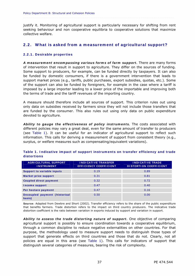
Policy Department B: Structural and Cohesion Policies _________________________________________________________________________________
PE 474.544 37
justify it. Monitoring of agricultural support is particularly necessary for shifting from rent seeking behaviour and non cooperative equilibria to cooperative solutions that maximize collective welfare.
2.2. What is asked from a measurement of agricultural support?
2.2.1. Desirable properties
A measurement encompassing various forms of farm support. There are many forms of intervention that result in support to agriculture. They differ on the sources of funding. Some support to producers, for example, can be funded directly by taxpayers. It can also be funded by domestic consumers, if there is a government intervention that leads to support market prices (e.g., tariffs, public purchases, export subsidies, quotas, etc.). Some of the support can also be funded by foreigners, for example in the case where a tariff is imposed by a large importer leading to a lower price of the importable and improving both the terms of trade and the tariff revenues of the importing country. A measure should therefore include all sources of support. This criterion rules out using only data on subsidies received by farmers since they will not include those transfers that are funded by the consumer. This also rules out using only data on public expenditure devoted to agriculture. Ability to gauge the effectiveness of policy instruments. The costs associated with different policies may vary a great deal, even for the same amount of transfer to producers (see Table 1). It can be useful for an indicator of agricultural support to reflect such information. This calls for deriving a measurement of support from consistent theory (e.g., surplus, or welfare measures such as compensating/equivalent variations).
Table 1. Indicative impact of support instruments on transfer efficiency and trade distortions
AGRICULTURAL SUPPORT INSTRUMENT
INDICATIVE TRANSFER EFFICIENCY COEFFICIENT
INDICATIVE TRADE DISTORTION COEFFICIENT
Support to variable inputs 0.19 0.89
Market price support 0.31 0.81
Coupled direct payment 0.32 0.72
Income support 0.47 0.40
Per hectare payment 0.47 0.16
Decoupled payment (historical basis)
0.50
0.00
Source: Adapted from Dewbre and Short (2002). Transfer efficiency refers to the share of the public expenditure that benefits farmers. Trade distortion refers to the impact on third country producers. The indicative trade distortion coefficient is the ratio between variation in exports induced by support and variation in support. Ability to assess the trade distorting nature of support. One objective of comparing agricultural support is possibly to ensure coordination towards a cooperative equilibrium, through a common discipline to reduce negative externalities on other countries. For that purpose, the methodology used to measure support needs to distinguish those types of support that generate effects on third countries and those that do not. Clearly, not all policies are equal in this area (see Table 1). This calls for indicators of support that distinguish several categories of measures, bearing the risk of complexity.
Comparative analysis of agricultural support within the major agricultural trading nations ___________________________________________________________________________________________
PE 474.544 38
An implementable measure. The practical implementability and the reliance on available data are important in constructing measures of agricultural support, in particular for measurements that are intended for international comparisons. Discrepancies between countries go beyond a problem of statistics as agriculture sometimes refers to different concepts (e.g., wine is an agricultural product in Europe, while it is considered as an industrial output in other countries where grapes are sold to wineries). International comparability requires the indicators to rely on easily available data, and therefore to be very simple. This rules out some of the indicators listed above, for example the Domestic Resource Cost, which is highly demanding on data (non traded inputs need to be factored out, technical coefficients are necessary as well as shadow exchange rates). A measurement on which it is easy to communicate. A frequent problem in the media is, for example, the erroneous interpretation of indicators of support. An example is the widely used PSE, a measurement of transfers to the farm sectors that includes production limiting payments or "virtuous" green payments, which are often used as a measurement of distorting support, and sometimes even a measurement of protection (see Appendix 2.1. for the list of categories that the OECD distinguishes for the PSE indicator only). Overall, a methodology for measuring agricultural support should:
Be able to encompass different forms of support. This calls for measures based on benchmarks approximating the situation without support (e.g., a set of undistorted prices). This is clearly a problem but other measures are unable to make meaningful comparisons when policies differ significantly;
Be consistent with microeconomic theory so as not to run into paradoxes for example when multiple prices vary in opposite ways;
Be simple, and parsimonious in data, so as to be used in the international forum. This implies that they do not rely on modelling results nor on elasticities;
Distinguish different categories of support, so as to reflect the degree of efficiency of transfers, and to reflect the trade distorting nature of the different forms of support.
Be easily understandable and have a clear interpretation.
Reconciling these different requirements is a challenge. An examination of the problems raised by the most common measurements of support may provide some elements for defining a methodology.
2.3. The pros and cons of the main measurements of farm support
2.3.1. Budget expenditure
For policy makers and in particular the Members of the European Parliament, decisions regarding agricultural support have a very practical aspect, i.e., the amount of the agricultural budget and the allocation of budgetary resources between the various forms of support. An analysis of the EU expenditure is particularly useful to assess agricultural support from the point of view of the taxpayers. The drawbacks of this approach are obvious. First, agricultural budgets include expenditure that does not benefit farmers much. This can be because budgets do not target farmers but instead another community (e.g., processors of agricultural products). Additional limitations arise when a large proportion of the payments can be "lost" in higher production costs (subsidies to products that have no comparative advantage), an increase in rents (when there is one essential factor with an
Policy Department B: Structural and Cohesion Policies _________________________________________________________________________________
PE 474.544 39
inelastic supply), or because these payments end up benefiting foreigners (e.g., export subsidies that cost the taxpayer but mostly benefit foreign consumers). That is, this approach focuses on the costs but give a poor image of the amount of money that farmers actually enjoy. Second, the budget approach is cost based but it only partially takes into account transfers from consumers, if there is, for example some price support.7
2.3.2. Subsidies received by farmers
Information on the payments received by farmers is the most direct way to assess how the transfers benefit producers. The information can be found in two sources, the economic accounts and farm level data. Economic accounts. Subsidies paid to farmers are reflected in the macroeconomic accounts of agriculture. In the EU this approach is particularly useful, since these accounts combine the subsidies that are funded by both the EU and the Member state budgets. Data from the economic accounts also make it possible to put in perspective agricultural support and agricultural income and to assess how dependent farmers are on subsidies. Within the EU, Eurostat makes these macroeconomic accounts consistent and comparable. At the international level, the fact that a number of countries follow United Nations accounting standards also allows for some comparisons. However, national economic accounts do not follow the same methodology across countries, when one needs to go into details such as agricultural subsidies (for example, the treatment of forestry differs between countries). Even for a given country, long term comparisons are difficult, due to changes in the classification. This is a particular problem with the EU national accounts for agriculture (for example, the introduction of subsidies in "basic prices" used in the EU system of national accounts has generated problems of consistency of comparisons both over time and across countries). Microeconomic sources provide an even more direct way to measure the payments received by farmers. EU Member States have the obligation to gather microeconomic data, which also provide information on the actual payments received by farmers. At the EU level, a centralized dataset gathers information on farm business accounts, the Farm Accounting Data Network also known as RICA or FADN. This source makes it possible to put in perspective the amount of subsidies received and some characteristics of the farms, including farm size, technico-economic orientation, etc. (EP, 2010). Approaches based on microeconomic sources nevertheless face limitations. First, like all payment based measures, they do not account for agricultural support in market prices. Information contained in the various microeconomic sources (e.g., farm business associations) is also very different across countries. International comparisons on a large sample of countries are practically impossible due to different accounting conventions. In the EU, FADN data are harmonized and comparable across Member States. Long time series comparisons are nevertheless difficult. There is a considerable turnover in the sample of the FADN and a problem of representativity in some Member States. Finally, access to these data is difficult due to restrictions linked to confidentiality protection.
7 Momagri (2011) proposed a set of "Indicateurs de soutiens globaux à la production agricole" in the EU and the
United States. Arguing that there is no satisfactory measure of a reference price for measuring price support, they consider only budgetary expenditure. We disagree with this point of view.
Comparative analysis of agricultural support within the major agricultural trading nations ___________________________________________________________________________________________
PE 474.544 40
2.3.3. Producer Support Estimates
30 years of improvement in the methodology. The main purpose of the OECD methodology is to monitor and evaluate developments in agricultural policy, to establish a common base for policy dialogue among countries, and to provide economic data to assess the effectiveness and efficiency of policies (OECD 2011a). The Secretariat has calculated indicators for OECD and an increasing number of non-OECD countries. The OECD indicators refer to a particular conception of “support”, which is understood as gross transfers to agriculture from consumers and taxpayers, arising from government policies supporting agriculture (see Appendix 2.1). In addition to budgetary expenditures, support includes estimated transfers which do not require actual monetary disbursements (e.g., credit concessions). It is important to understand that the OECD indicators measure policy transfers, not production or trade effects. In particular, they are of little help in distinguishing policy interventions that are designed to respond to market failures and those that are designed to provide rents to producers. Methodological issues have been discussed since the early 1980s when the Secretariat started to calculate Producer Subsidy Equivalents (the predecessor of the current Producer Support Estimate).8 Many of the recent criticisms made to the OECD methodology have actually been raised some 20 years ago. In many cases, possible solutions were debated within the proper committees. Some have been implemented, which led to a major change in the methodology in the late 1980s.9 The OECD indicators. The PSE includes two components. The first one is the transfer directly linked to a particular output, either through a product specific direct payment or market price support (the OECD category of single commodity transfers does not necessarily correspond to the WTO notion of product-specific support). The second one is the non-product specific transfers. The OECD classification distinguishes various categories of transfers, those that subsidize inputs, that depend on the number of hectares or animal heads, on current income, or on historical references, those granted under the condition that production takes place, and those that do not require production (see Annex 2.2). This classification attempts to reflect the less coupled nature of the support, as well as the support that is conditional on restructuring production or withdrawing resources from agriculture. In addition to the PSE, which measures support received by individual farmers, OECD indicators include the CSE and the TSE. The CSE is an estimate of the support (often negative) to the users of the agricultural products. The TSE is an estimate of total support to the agricultural sector (see a definition of the indicators calculated by the OECD in Appendix 2.1.). The TSE is constructed by adding the general expenses related to the
8 The Producer Subsidy Equivalent was initially defined as the payment that would be required to compensate
farmers for the loss of income resulting from the removal of a given policy measure (OECD, 1987). It followed the pioneering works of Corden (1971) and Josling (1973).
9 In particular the PSE was redefined in 1990 as the annual monetary value of gross transfers from consumers and taxpayers to agricultural producers, measured at the farm-gate level, arising from policy measures that support agriculture, regardless of their nature, objectives or impact on farm production or income. In 1999 Producer Support Estimates replaced the Producer Subsidy Equivalent. Support granted through general services, which were included in the PSE, were taken out in a separate category, the GSSE. In 2007, changes in the methodology led to new classifications, and to replace the single commodity PSEs by categories such as Single Commodity Transfers, Group Commodity Transfers, and All Commodity Transfers which are more in line with the reforms that OECD countries adopted in the late 1990s and the 2000s. A history of the PSE methodology can be found in Cahill and Legg (1989). The conventions and methods used have been frequently updated, and are fairly transparent, being published on the internet (OECD 2011a). See also OECD (2009) and Jones (2010).
Policy Department B: Structural and Cohesion Policies _________________________________________________________________________________
PE 474.544 41
agricultural sector and the amount of transfers from taxpayers to consumers implied in food aid and assistance to the disposal of agricultural production to the PSE. These indicators monitor and aggregate transfers between consumers, taxpayers and producers (see section 1.3.3). Evaluations are made in a static framework, considering that domestic supply and demand as well as world prices are exogenous. The advantage of this crude simplification is that no data is needed regarding behavioural parameters such as supply elasticities. The issue of market price support. A major advantage of the PSE measurement is that it accounts for the support that is paid by consumers through higher guaranteed prices. This is clearly an approach preferable to using only budgetary data. The way the OECD estimates price support, however, relies on particular assumptions. In order to keep the indicator robust and avoid using econometric models, the benchmark used for the counterfactual scenario (i.e., without government intervention on prices) is the world price. Market Price Support (MPS) is constructed as the quantity produced times the difference between producer price and border price. Adjustment for transport costs makes prices comparable. Double counting is avoided when measures supporting domestic prices also have some budgetary costs (e.g., storage costs, subsidized exports). Focusing on the impact on prices rather than on the budget cost is consistent with economic theory.10 The PSE methodology makes it possible to account for different forms of support, including the one provided by production quotas and guaranteed prices, for example. However, in practice, there has been much controversy regarding the use of world prices as references.11 Many of the criticisms on the estimation of MPS by the OECD are somewhat misplaced. The PSE is not intended to measure a welfare variation. The objective is to measure transfers between agents in a static framework, and it is clearly stated that this measure is ceteris paribus, i.e., without attempting to take into account changes in supply and demand induced by farm support policies (Tangermann, 2003). Indeed, any attempt to do so with a simple indicator would be hopeless, unless one uses a full blown model that would make it possible to compare the current situation to a counterfactual one without support, accounting for general equilibrium effects (e.g., distribution of tariff revenues, terms of trade, macroeconomic linkages, etc.). It would also be necessary to consider the positive and negative externalities in the economy that are regulated by government intervention. For this reason the OECD methodology can be seen as a good compromise between theoretical consistency and implementability, provided that one keeps in mind its limited objective. It nevertheless has some caveats. Caveats of the PSE measures. Many authors, and the Member State delegations, have expressed criticisms on several aspects of the PSE approaches. Among the references, one could quote McClatchy (1987), Peters (1989); Byerlee and Morris (1993), Masters (1993), Mervoyer et al (2001), Doyon et al (2002); Haniotis and Bascou (2003), Oskam and Meester (2006), Gohin (2006); Tangermann (2008), etc. While some of these criticisms have been addressed and the methodology has been changed, some concerns persist. The OECD Secretariat stresses the consistency of the PSE with underlying economic theory. It is true that the Market Price Support component of the PSE has a welfare-theoretic basis, 10 It is noteworthy that the costs of public storage are included in other indicators of general services (GSSE) and
that tariffs revenues are also accounted for (in the TSE). 11 Vernières(1984), Byerlee and Morris (1993), Buckwell (1997), Doyon et al. (2002), Momagri, (2011) are only
a few of the many possible references critical on the use of world prices.
Comparative analysis of agricultural support within the major agricultural trading nations ___________________________________________________________________________________________
PE 474.544 42
since it measures the monetary value of the pre-reform aggregate distortion resulting from agricultural policy. However, by summing all the monetary values of a variety of subsidies without any weights, the PSE adopts a questionable metric. In taking the sum of direct transfers and price support, the PSE measure totals over two very different categories. The indicator therefore sums terms that have very different welfare effects. The OECD approach includes a detailed classification of the farm support by types of measures (Annex 2.1). This is consistent with the need to distinguish between farm support that is efficiently transferred to producers and the support provided by less effective policies. However, the OECD classification considers the way the measures are implemented rather than the objective of the support. As a result, for example, the Secretariat includes in the same category the EU payments that resulted from the 1992 reform, the support to areas with natural handicap, and most of the environmental payments in the same category, even though their objective, but also the production and consumption incentives they generate, differ significantly. In particular, environmental payments and payments for reducing risk are not well isolated from other, often more distorting, payments (Jones, 2010). Inevitably, there is a grey area on which policies should be included in the measurement of agricultural support. For example, subsidies and tax rebates for biofuel users have amounted to several billion dollars worldwide, and they lead to higher agricultural prices (Steenblik 2007). The US food stamp and other nutrition programs exceed US$50 billion annually, also driving up agricultural prices (EP, 2007). Neither of them is included in the calculation of the PSE.12 There are good reasons for that. The PSE is supposed to measure the impact on producers in one country of the actions of their own government. Because biofuel subsidies and mandates lead to a higher world price, by construction this does not translate into a higher PSE. Indeed, an increase in the demand for feedstock caused by a domestic food aid program, a biofuel mandate, or a restriction on production (set aside, conservation reserve, etc.) also has benefits for other producers. The convention of excluding biofuel policies from the PSE calculation is defendable, as explained by Josling et al. (2010). However, because of the level of the transfers, and the role played by both food aid and biofuel programs to support agricultural markets, the PSE ignores a potentially large form of agricultural support. The MPS is calculated on a list of products that is country specific and the corresponding support is extrapolated to other products. In the case of the EU, it tends to overestimate the actual support given so that the residual products include mainly products that benefit from little support, such as fruits and vegetables. In order to solve this problem, the OECD Secretariat has expanded the list of products for which MPS is calculated, which has reduced the bias, but it has not fully disappeared. In the EU, almost a fifth of the commodity specific transfers are based on estimates for non PSE commodities. For some commodities, the reference prices used in the PSE calculation are questionable. Because fluid milk is not traded internationally, this has long been a problem for dairy products. The current calculation of the market price support for milk relies on the price differential observed for tradable products, i.e., butter, skimmed milk powder and cheese. This price differential is adjusted to generate a virtual reference price for milk. The methodology is transparent and has been discussed extensively within OECD committees
12 The US food aid progamme is included in the GSSE and food aid programs that are associated with measures
that support agriculture, e.g., distribution of government stocks acquired in the context of market interventions, are included in the CSE.
Policy Department B: Structural and Cohesion Policies _________________________________________________________________________________
PE 474.544 43
but overall, it calls for a number of parameters whose reliability is uncertain.13 This is particularly the case for milk, where processing margins, transportation costs and quality differences need to be approximated to calculate the reference price at the farm gate level. It is also the case for beef (quality differences, transportation costs, handling margins, etc.). On the practical side, it is unclear how the OECD Secretariat has been able to obtain information on all agricultural support. Support granted at the regional level (e.g., Italian, Canadian, Chinese provinces, US or Brazilian states, etc.) are not always communicated by the central government. For some services, the reporting is left to Member states, which may exclude some particular measures on a rather arbitrary basis. A classic criticism to the PSE measure is it depends on prices that are affected by exogenous factors. Variations over time in the PSE reflect not only changes in policy settings but also changing world market conditions and exchange rates. This has long been a subject of discomfort for the Member States delegates to the OECD and has triggered an intense debate over the years to find solutions to this issue. Sensitivity of the PSEs to exchange rates and world price fluctuations has led delegations to the WTO to adopt fixed references for both world prices and exchange rates in the AMS, the measurement adopted in multilateral negotiations. This turned out to be a poor decision as explained below. This issue motivates the choice, for the methodology adopted in this report, to define an alternative version of the PSE, relying on purchasing power standards.
2.3.4. The Aggregate Measurement of Support
The 1994 Agreement on Agriculture distinguishes among several categories of agricultural (domestic) support. Agricultural support through measures that generate no or minimal trade distortions and that meet certain criteria are classified in a category often unofficially called Green Box. It includes general services funded by public money but not involving payments to producers. Payments to producers can qualify for the green box if they meet all the specific criteria under one of several headings, such as decoupled income support, income safety-nets, environmental programs, or regional assistance. The specific criteria under each heading are expressed such that they, when combined, allow payments to qualify under the green box heading only if they are relatively decoupled from production. Payments that do not qualify for the Green Box may qualify for the Blue Box if they meet the relevant criteria, which include that they are made under production-limiting programmes and relate to a fixed parameter, such area or number of livestock heads. Certain investment subsidies and input subsidies in developing countries can be classified as Development Programme support. All other support than green box, blue box, and development program support is usually referred to as Amber Box support. Since the criteria for green box and blue box support tend to capture measures that provide support with relatively small effects on production and trade, the amber box support is considered to be of a relatively distorting nature. It includes programs such as price support and subsidies directly linked to current output or inputs used. Examples are US price supports for dairy and sugar, US loan deficiency payments or marketing loans for grain, oilseed, and 13 The convention of taking a fluid milk price in a reference country with no support policy was abandoned in
2004. Indeed, in all countries that are large enough it seems impossible to find a country where there is neither significant government support nor monopoly or monopsony power that distorts prices (e.g., New Zealand). It is noteworthy that, in the 1990s, the US Department of Agriculture calculated its own PSEs and, at the time, chose to rely on a combination of the international price of milk powder and butter. This approach was found to rely too much on markets that were heavily distorted by export subsidies and was not endorsed by the OECD Secretariat. Because the PSEs using the new methodology were extrapolated back to 1986, they also rely on world prices for milk powder and butter that were heavily distorted by export subsidies (subsidised EU exports of milk powder accounted for more than two thirds of the world market in the 1980s).
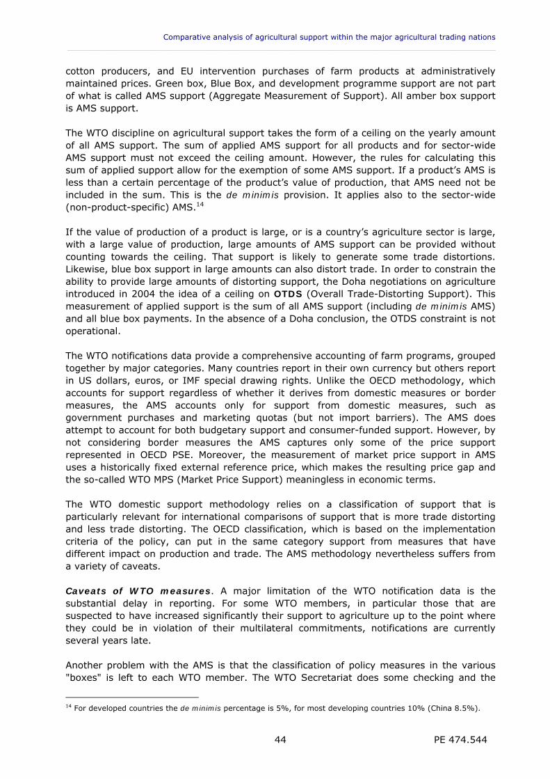
Comparative analysis of agricultural support within the major agricultural trading nations ___________________________________________________________________________________________
PE 474.544 44
cotton producers, and EU intervention purchases of farm products at administratively maintained prices. Green box, Blue Box, and development programme support are not part of what is called AMS support (Aggregate Measurement of Support). All amber box support is AMS support. The WTO discipline on agricultural support takes the form of a ceiling on the yearly amount of all AMS support. The sum of applied AMS support for all products and for sector-wide AMS support must not exceed the ceiling amount. However, the rules for calculating this sum of applied support allow for the exemption of some AMS support. If a product’s AMS is less than a certain percentage of the product’s value of production, that AMS need not be included in the sum. This is the de minimis provision. It applies also to the sector-wide (non-product-specific) AMS.14 If the value of production of a product is large, or is a country’s agriculture sector is large, with a large value of production, large amounts of AMS support can be provided without counting towards the ceiling. That support is likely to generate some trade distortions. Likewise, blue box support in large amounts can also distort trade. In order to constrain the ability to provide large amounts of distorting support, the Doha negotiations on agriculture introduced in 2004 the idea of a ceiling on OTDS (Overall Trade-Distorting Support). This measurement of applied support is the sum of all AMS support (including de minimis AMS) and all blue box payments. In the absence of a Doha conclusion, the OTDS constraint is not operational. The WTO notifications data provide a comprehensive accounting of farm programs, grouped together by major categories. Many countries report in their own currency but others report in US dollars, euros, or IMF special drawing rights. Unlike the OECD methodology, which accounts for support regardless of whether it derives from domestic measures or border measures, the AMS accounts only for support from domestic measures, such as government purchases and marketing quotas (but not import barriers). The AMS does attempt to account for both budgetary support and consumer-funded support. However, by not considering border measures the AMS captures only some of the price support represented in OECD PSE. Moreover, the measurement of market price support in AMS uses a historically fixed external reference price, which makes the resulting price gap and the so-called WTO MPS (Market Price Support) meaningless in economic terms. The WTO domestic support methodology relies on a classification of support that is particularly relevant for international comparisons of support that is more trade distorting and less trade distorting. The OECD classification, which is based on the implementation criteria of the policy, can put in the same category support from measures that have different impact on production and trade. The AMS methodology nevertheless suffers from a variety of caveats. Caveats of WTO measures. A major limitation of the WTO notification data is the substantial delay in reporting. For some WTO members, in particular those that are suspected to have increased significantly their support to agriculture up to the point where they could be in violation of their multilateral commitments, notifications are currently several years late. Another problem with the AMS is that the classification of policy measures in the various "boxes" is left to each WTO member. The WTO Secretariat does some checking and the
14 For developed countries the de minimis percentage is 5%, for most developing countries 10% (China 8.5%).
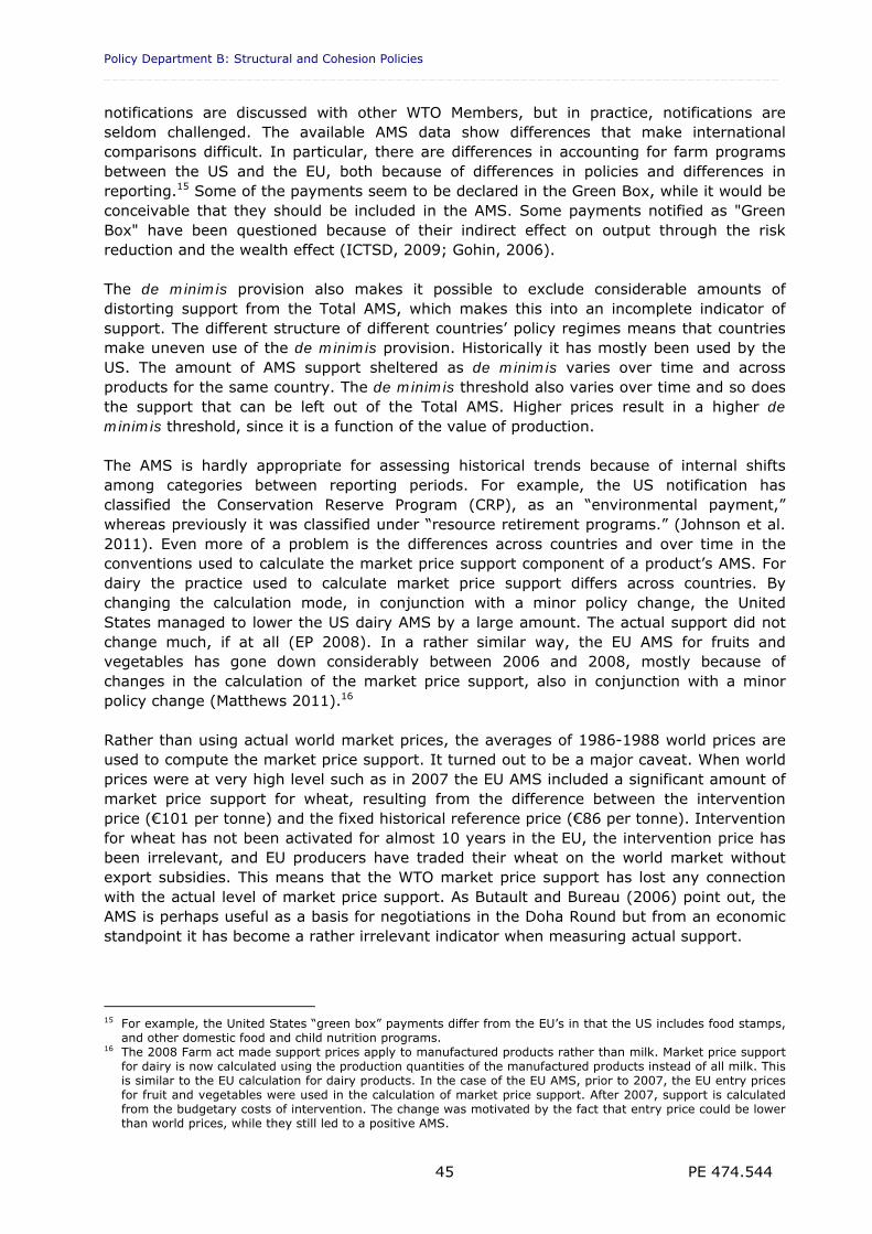
Policy Department B: Structural and Cohesion Policies _________________________________________________________________________________
PE 474.544 45
notifications are discussed with other WTO Members, but in practice, notifications are seldom challenged. The available AMS data show differences that make international comparisons difficult. In particular, there are differences in accounting for farm programs between the US and the EU, both because of differences in policies and differences in reporting.15 Some of the payments seem to be declared in the Green Box, while it would be conceivable that they should be included in the AMS. Some payments notified as "Green Box" have been questioned because of their indirect effect on output through the risk reduction and the wealth effect (ICTSD, 2009; Gohin, 2006). The de minimis provision also makes it possible to exclude considerable amounts of distorting support from the Total AMS, which makes this into an incomplete indicator of support. The different structure of different countries’ policy regimes means that countries make uneven use of the de minimis provision. Historically it has mostly been used by the US. The amount of AMS support sheltered as de minimis varies over time and across products for the same country. The de minimis threshold also varies over time and so does the support that can be left out of the Total AMS. Higher prices result in a higher de minimis threshold, since it is a function of the value of production. The AMS is hardly appropriate for assessing historical trends because of internal shifts among categories between reporting periods. For example, the US notification has classified the Conservation Reserve Program (CRP), as an “environmental payment,” whereas previously it was classified under “resource retirement programs.” (Johnson et al. 2011). Even more of a problem is the differences across countries and over time in the conventions used to calculate the market price support component of a product’s AMS. For dairy the practice used to calculate market price support differs across countries. By changing the calculation mode, in conjunction with a minor policy change, the United States managed to lower the US dairy AMS by a large amount. The actual support did not change much, if at all (EP 2008). In a rather similar way, the EU AMS for fruits and vegetables has gone down considerably between 2006 and 2008, mostly because of changes in the calculation of the market price support, also in conjunction with a minor policy change (Matthews 2011).16 Rather than using actual world market prices, the averages of 1986-1988 world prices are used to compute the market price support. It turned out to be a major caveat. When world prices were at very high level such as in 2007 the EU AMS included a significant amount of market price support for wheat, resulting from the difference between the intervention price (€101 per tonne) and the fixed historical reference price (€86 per tonne). Intervention for wheat has not been activated for almost 10 years in the EU, the intervention price has been irrelevant, and EU producers have traded their wheat on the world market without export subsidies. This means that the WTO market price support has lost any connection with the actual level of market price support. As Butault and Bureau (2006) point out, the AMS is perhaps useful as a basis for negotiations in the Doha Round but from an economic standpoint it has become a rather irrelevant indicator when measuring actual support.
15 For example, the United States “green box” payments differ from the EU’s in that the US includes food stamps,
and other domestic food and child nutrition programs. 16 The 2008 Farm act made support prices apply to manufactured products rather than milk. Market price support
for dairy is now calculated using the production quantities of the manufactured products instead of all milk. This is similar to the EU calculation for dairy products. In the case of the EU AMS, prior to 2007, the EU entry prices for fruit and vegetables were used in the calculation of market price support. After 2007, support is calculated from the budgetary costs of intervention. The change was motivated by the fact that entry price could be lower than world prices, while they still led to a positive AMS.
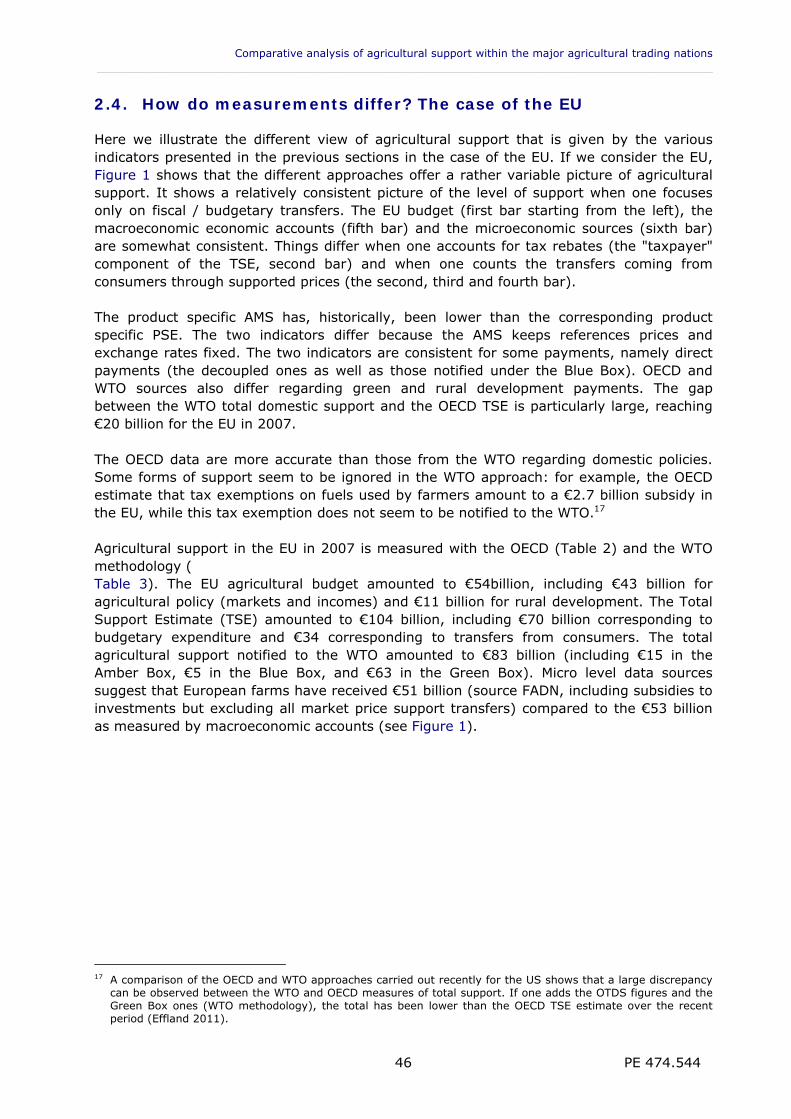
Comparative analysis of agricultural support within the major agricultural trading nations ___________________________________________________________________________________________
PE 474.544 46
2.4. How do measurements differ? The case of the EU
Here we illustrate the different view of agricultural support that is given by the various indicators presented in the previous sections in the case of the EU. If we consider the EU, Figure 1 shows that the different approaches offer a rather variable picture of agricultural support. It shows a relatively consistent picture of the level of support when one focuses only on fiscal / budgetary transfers. The EU budget (first bar starting from the left), the macroeconomic economic accounts (fifth bar) and the microeconomic sources (sixth bar) are somewhat consistent. Things differ when one accounts for tax rebates (the "taxpayer" component of the TSE, second bar) and when one counts the transfers coming from consumers through supported prices (the second, third and fourth bar). The product specific AMS has, historically, been lower than the corresponding product specific PSE. The two indicators differ because the AMS keeps references prices and exchange rates fixed. The two indicators are consistent for some payments, namely direct payments (the decoupled ones as well as those notified under the Blue Box). OECD and WTO sources also differ regarding green and rural development payments. The gap between the WTO total domestic support and the OECD TSE is particularly large, reaching €20 billion for the EU in 2007. The OECD data are more accurate than those from the WTO regarding domestic policies. Some forms of support seem to be ignored in the WTO approach: for example, the OECD estimate that tax exemptions on fuels used by farmers amount to a €2.7 billion subsidy in the EU, while this tax exemption does not seem to be notified to the WTO.17 Agricultural support in the EU in 2007 is measured with the OECD (Table 2) and the WTO methodology ( Table 3). The EU agricultural budget amounted to €54billion, including €43 billion for agricultural policy (markets and incomes) and €11 billion for rural development. The Total Support Estimate (TSE) amounted to €104 billion, including €70 billion corresponding to budgetary expenditure and €34 corresponding to transfers from consumers. The total agricultural support notified to the WTO amounted to €83 billion (including €15 in the Amber Box, €5 in the Blue Box, and €63 in the Green Box). Micro level data sources suggest that European farms have received €51 billion (source FADN, including subsidies to investments but excluding all market price support transfers) compared to the €53 billion as measured by macroeconomic accounts (see Figure 1).
17 A comparison of the OECD and WTO approaches carried out recently for the US shows that a large discrepancy
can be observed between the WTO and OECD measures of total support. If one adds the OTDS figures and the Green Box ones (WTO methodology), the total has been lower than the OECD TSE estimate over the recent period (Effland 2011).
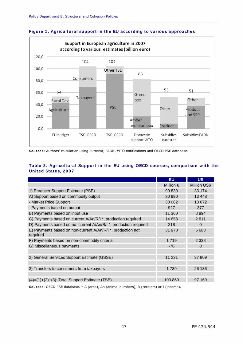
Policy Department B: Structural and Cohesion Policies _________________________________________________________________________________
PE 474.544 47
Figure 1. Agricultural support in the EU according to various approaches
Sources: Authors' calculation using Eurostat, FADN, WTO notifications and OECD PSE database.
Table 2. Agricultural Support in the EU using OECD sources, comparison with the United States, 2007
EU US Million € Million US$ 1) Producer Support Estimate (PSE) 90 839 33 174 A) Support based on commodity output 30 990 13 448 - Market Price Support 30 062 13 072 - Payments based on output 927 377 B) Payments based on input use 11 360 8 894 C) Payments based on current A/An/R/I *, production required 14 658 2 811 D) Payments based on no current A/An/R/I *, production required 218 0 E) Payments based on non-current A/An/R/I *, production not required
31 970 5 683
F) Payments based on non-commodity criteria 1 719 2 338 G) Miscellaneous payments -76 0 2) General Services Support Estimate (GSSE) 11 231 37 809 3) Transfers to consumers from taxpayers 1 789 26 186 (4)=(1)+(2)+(3): Total Support Estimate (TSE) 103 859 97 169
Sources: OECD PSE database. * A (area), An (animal numbers), R (receipts) or I (income).
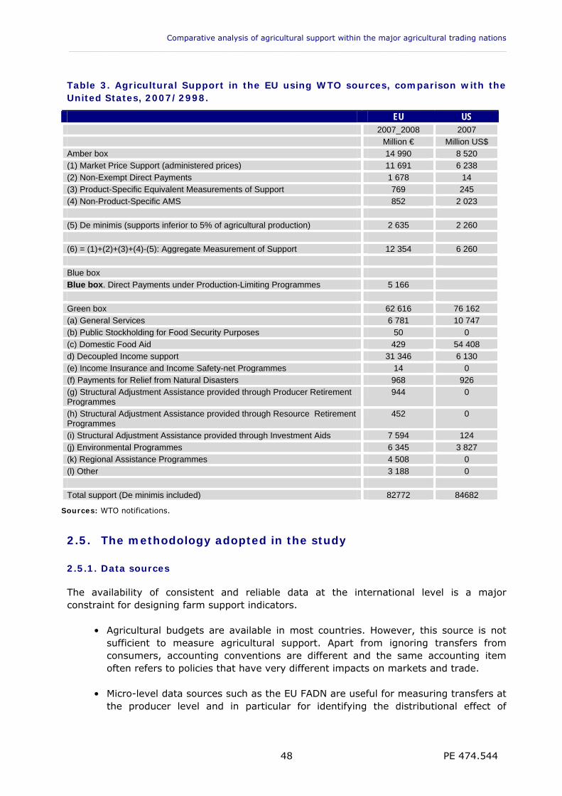
Comparative analysis of agricultural support within the major agricultural trading nations ___________________________________________________________________________________________
PE 474.544 48
Table 3. Agricultural Support in the EU using WTO sources, comparison with the United States, 2007/2998.
EU US 2007_2008 2007
Million € Million US$
Amber box 14 990 8 520
(1) Market Price Support (administered prices) 11 691 6 238
(2) Non-Exempt Direct Payments 1 678 14
(3) Product-Specific Equivalent Measurements of Support 769 245
(4) Non-Product-Specific AMS 852 2 023
(5) De minimis (supports inferior to 5% of agricultural production) 2 635 2 260
(6) = (1)+(2)+(3)+(4)-(5): Aggregate Measurement of Support 12 354 6 260
Blue box Blue box. Direct Payments under Production-Limiting Programmes 5 166
Green box 62 616 76 162
(a) General Services 6 781 10 747
(b) Public Stockholding for Food Security Purposes 50 0
(c) Domestic Food Aid 429 54 408
d) Decoupled Income support 31 346 6 130
(e) Income Insurance and Income Safety-net Programmes 14 0
(f) Payments for Relief from Natural Disasters 968 926
(g) Structural Adjustment Assistance provided through Producer Retirement Programmes
944 0
(h) Structural Adjustment Assistance provided through Resource Retirement Programmes
452 0
(i) Structural Adjustment Assistance provided through Investment Aids 7 594 124
(j) Environmental Programmes 6 345 3 827
(k) Regional Assistance Programmes 4 508 0
(l) Other 3 188 0
Total support (De minimis included) 82772 84682
Sources: WTO notifications.
2.5. The methodology adopted in the study
2.5.1. Data sources
The availability of consistent and reliable data at the international level is a major constraint for designing farm support indicators.
• Agricultural budgets are available in most countries. However, this source is not
sufficient to measure agricultural support. Apart from ignoring transfers from consumers, accounting conventions are different and the same accounting item often refers to policies that have very different impacts on markets and trade.
• Micro-level data sources such as the EU FADN are useful for measuring transfers at
the producer level and in particular for identifying the distributional effect of
Policy Department B: Structural and Cohesion Policies _________________________________________________________________________________
PE 474.544 49
agricultural support. Comparison with third countries, however, is hardly possible because of incoherence in accounting rules and data collection.
• WTO notifications on domestic support are available for 126 geographical entities
(153 Member States but 126 given that EU notifications are for all EU27 Member states and Switzerland and Liechtenstein as a single entity). The annual notification is mandatory since 1995, but some Member states are late in providing information on their domestic support. Because of the uncertainty on how the countries have notified their subsidies, this source is not fully reliable when one wants to compare various forms of support across countries.
The OECD database is the primary source of information for this work. It includes the budgetary data, which has largely been made comparable thanks to decades of work by the Secretariat under the control of national governments. The estimates of market price support are controversial, but they are transparent and well-documented. The dataset provides information on the OECD members, i.e., 14 entities including the EU, Australia, Canada, Switzerland, Iceland, Japan, Korea, Mexico, Norway, Turkey, USA, Israel, Chile, between 1986 and 2010, as well as some transition countries between 1995 and 2010 (Brazil, China, Russia, Ukraine, South Africa).
2.5.2. Indicators
Section 2.3.4 showed that the AMS is hardly suited for economic comparisons of agricultural support across countries, or even over time. The concept has lost connection with current markets due to the fixed reference price. Notifications are too discretionary and the classification of support lack consistency both across countries and over time. Overall, the AMS is more suited to the monitoring of compliance with policy commitments. The OECD methodology is more in line with the economic reality, as the conventions used are more consistent and there is a more coherent effort to gather all subsidies and payments. Accounting for market price support remains necessary for meaningful comparisons across countries. While some of the OECD methodology is not fully satisfactory (e.g., the choice of particular reference prices), ignoring market price support is clearly not an acceptable solution. Compared to the OECD methodology, we believe that there is an interest in defining aggregates that provide more information on the efficiency and distorting nature of various forms of support. The OECD PSE sub aggregates provide little information on this. By contrast, the WTO classification is more oriented towards assessing the trade distorting nature of the support. We will use an ad hoc classification of the payments that makes use of the information provided on the nature of the payments (see Annex 2.1) in a way that attempts to distinguish instruments on the basis of their distorting nature. Another change relative to the OECD methodology is that we will present the classification of payments in a simpler way, focusing on the main payments that account for the bulk of transfers in each country. Finally, a major change is that we will use real values in the comparisons, requiring computation of purchasing power parities.
2.5.3. Purchasing power parities
The exchange rate issue. The measurement of support across countries and time is sensitive to variations in exchange rates. Exchange rate fluctuations can affect the measurement of support when the agricultural policy takes the form of price support or a
Comparative analysis of agricultural support within the major agricultural trading nations ___________________________________________________________________________________________
PE 474.544 50
subsidy fully coupled with output, as it affects the level of border prices after they are converted into national currency. Border prices increase in a country where the currency is depreciating and decrease in a country where the currency is appreciating. If two countries maintain the same level of price support for a given agricultural commodity, the support will fall in the country whose currency depreciates and rise in the second case. Note that this exchange rate effect is not something "artificial". In “unprotected” sectors, the devaluation of a country’s currency stimulates the competitiveness of that country’s export sectors, whereas a revaluation penalizes them. Countries with an undervalued currency have fewer constraints on supporting their farm prices. However, in international comparisons, exchange rate variations raise difficulties. For example, if one looks carefully at the work published annually by the OECD on the measurement of agricultural support, the very central message that results from the indicators expressed in dollars can contradict that of the indicators measured in euro. Here, we use a measure based on the Purchasing Power Parity (PPP) of the currencies. Butault (2011) presents extensive discussion of how PPPs can help international comparisons of agricultural support. The fact that one dollar can be exchanged for one euro at the nominal exchange rate does not mean that it is possible to buy the same basket of goods with one dollar in the US as with one euro in the EU. The exchange rate that ensures that the same basket of good can be purchased in both countries is the PPP (which can be calculated for a specific basket of goods, a well known indicator is the simple "Big Mac" index published annually by the magazine The Economist since 1986, which relies on the comparison of a simple, homogenous good, a hamburger). In particular a PPP can be constructed for a basket of agricultural goods, so as to construct a spatial price index for agricultural products. In practice, PPPs are computed by several international organisations for a basket of goods that, most of the time, reflect the patterns of consumption of the average consumer.18 One use of these PPPs based on the basket of goods that is either representative of final consumer's demand, or of the entire economy (the goods that reflect the Gross Domestic Product or GDP) are often use as a benchmark exchange rate to assess the over or under valuation of a currency at a point in time. In spite of the underlying assumptions, in this study we will consider that a currency is undervalued if its market price is lower than its real purchasing power and overvalued if the opposite is true. That is, we use the GDP-based PPP as a long term equilibrium exchange rate.19 In other sections of the study we will also construct PPPs that are specific to the agricultural sector, relying on a basket of 15 common agricultural commodities, so as to compare output prices and measure the real value of output across countries (Bureau and Butault 1992). This leads to calculation of spatial price indexes across countries and spatial volume indexes specific to a basket of goods representing agricultural products 18 The OECD, Eurostat and the World Bank base their calculations of purchasing power parities on all the
commodities that make up each country’s GDP. This provides an indicator that can be used to deflate, across countries, economic magnitudes expressed in national currency, in order to evaluate them in terms of purchasing power. For example, the World Bank publishes the gross national income (GNI) per capita for the different countries in current dollars and in current international dollars (PPP). These two denominations result in different wealth rankings for countries.
19 Note that there are many other ways to define a benchmark exchange rate than the PPP (for example one might define an exchange rate that would keep trade balanced). The PPP as a long term reference exchange rate is questionable. In particular the relevance of PPP as a benchmark to gauge the appreciation of a currency is uncertain, in particular in countries where there is a large informal sector.
Policy Department B: Structural and Cohesion Policies _________________________________________________________________________________
PE 474.544 51
The case of the PSE. For comparison between countries, it is tempting to express the PSE of each county in a common currency. For example, the OECD publishes support indicators such as the PSE in both US dollars and in euro. However, expressing a country’s PSE in another country’s currency unit is misleading. As a general rule, for the same level of support in a country, the PSE will increase if it is converted into a depreciating currency and fall if it is converted into an appreciating currency. While it is understandable that the PSE in one country falls if the currency of this country depreciates, the issue here is different: if the choice of a common currency leads to variations in the PSE that are not caused by the domestic policy of the country, it is a measurement bias. In addition, the aggregation of the PSE on a group of countries such as the EU, or the OECD as a whole, is particularly sensitive to the choice of such a numeraire. Again, when the OECD Secretariat uses the currency of a particular country, the dollar or the euro, as a common currency to construct the OECD aggregate PSE, the results, in particular changes over time, depend on the choice of currency, e.g., euro or US dollar. The PSE comprises transfers from taxpayers and consumers to agricultural producers. It is therefore appropriate to assess the evolution of the PSE over time for a given country, or between countries at a given point in time, in terms of purchasing power, i.e., in real terms. In this case, the appropriate price indices for deflating the PSE in each country over time are those that allow for inflation, that is to say the variation in the purchasing power of these transfers: the GDP price index or the consumer price index. Expressing support in nominal national currencies makes little sense, especially in the long term, as inflation rates vary over time (in every country) and between countries. One must use fixed-based PPPs for international comparisons (Schreyer et al., 2002). If we use fixed-based PPPs for a benchmark year and the GDP based price index over time, neither the choice of the country for which GDP purchasing power parities (GDP PPPs) are calculated, nor the choice of the year of the rate, affects the resulting trends in the value of support. The PPP rate between two countries evolves as follows:
B
tt
AttBA
tBA
t PI
PIPPPPPP
1/
1///1 .
,
where PPPA/B is the PPP between two countries A and B, and PI is the GDP price index between t and t+1.Obviously the absolute value of support varies with the choice of reference PPP rate but, when it is expressed in indices, support trends are the same irrespective of which base country and year are chosen. Specific PPPs for constructing price and quantity indexes for agricultural products. It is useful to construct PPPs for a specific basket of goods, such as agricultural products. This makes it possible to construct price and quantity index for, say, output, and to make international comparisons. The construction of such indexes has raised controversial methodological issues (see Deaton and Heston, 2009 for a recent synthesis). Indeed, no index satisfies all the properties that are considered as desirable by an axiomatic approach which provides rigorous guidelines for choosing a particular methodology (Diewert, 2003). Desirable properties include additivity, reversibility, transitivity and equicharacteristicity. Equicharacteristicity means that no country is privileged in the weighting. Another approach, the economic approach, proposes to choose an aggregation formula based on the economic properties of the underlying producer technology or consumer preferences. Building on previous studies involving some of the authors of this report (Bureau et al 1992, Ball et al., 1997), and backed by academic literature on both the axiomatic and the
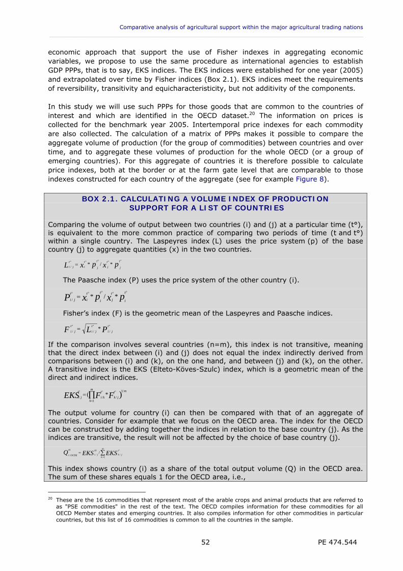
Comparative analysis of agricultural support within the major agricultural trading nations ___________________________________________________________________________________________
PE 474.544 52
economic approach that support the use of Fisher indexes in aggregating economic variables, we propose to use the same procedure as international agencies to establish GDP PPPs, that is to say, EKS indices. The EKS indices were established for one year (2005) and extrapolated over time by Fisher indices (Box 2.1). EKS indices meet the requirements of reversibility, transitivity and equicharacteristicity, but not additivity of the components. In this study we will use such PPPs for those goods that are common to the countries of interest and which are identified in the OECD dataset.20 The information on prices is collected for the benchmark year 2005. Intertemporal price indexes for each commodity are also collected. The calculation of a matrix of PPPs makes it possible to compare the aggregate volume of production (for the group of commodities) between countries and over time, and to aggregate these volumes of production for the whole OECD (or a group of emerging countries). For this aggregate of countries it is therefore possible to calculate price indexes, both at the border or at the farm gate level that are comparable to those indexes constructed for each country of the aggregate (see for example Figure 8).
BOX 2.1. CALCULATING A VOLUME INDEX OF PRODUCTION SUPPORT FOR A LIST OF COUNTRIES
Comparing the volume of output between two countries (i) and (j) at a particular time (t°), is equivalent to the more common practice of comparing two periods of time (t and t°) within a single country. The Laspeyres index (L) uses the price system (p) of the base country (j) to aggregate quantities (x) in the two countries.
pxpxLt
j
t
j
t
j
t
i
t
ji
*/*/
The Paasche index (P) uses the price system of the other country (i).
pxpxPt
i
t
j
t
i
t
i
t
ji
*/*/
Fisher’s index (F) is the geometric mean of the Laspeyres and Paasche indices.
PLFt
ji
t
ji
t
ji
///
*
If the comparison involves several countries (n=m), this index is not transitive, meaning that the direct index between (i) and (j) does not equal the index indirectly derived from comparisons between (i) and (k), on the one hand, and between (j) and (k), on the other. A transitive index is the EKS (Elteto-Köves-Szulc) index, which is a geometric mean of the direct and indirect indices.
)/1
/1
//*(
mt
jk
m
k
t
ki
t
ji FFEKS
The output volume for country (i) can then be compared with that of an aggregate of countries. Consider for example that we focus on the OECD area. The index for the OECD can be constructed by adding together the indices in relation to the base country (j). As the indices are transitive, the result will not be affected by the choice of base country (j).
m
k
t
jk
t
ji
t
OCDEi EKSEKSQ1
/
0
/
0
//
This index shows country (i) as a share of the total output volume (Q) in the OECD area. The sum of these shares equals 1 for the OECD area, i.e.,
20 These are the 16 commodities that represent most of the arable crops and animal products that are referred to
as "PSE commodities" in the rest of the text. The OECD compiles information for these commodities for all OECD Member states and emerging countries. It also compiles information for other commodities in particular countries, but this list of 16 commodities is common to all the countries in the sample.
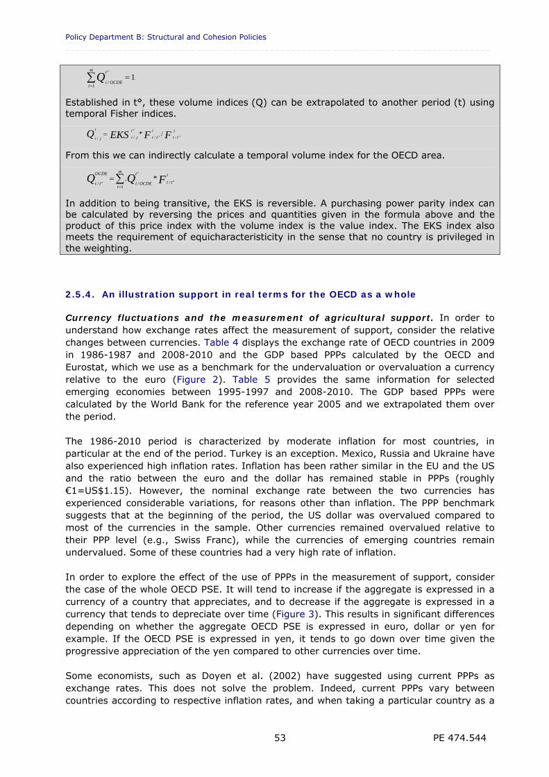
Policy Department B: Structural and Cohesion Policies _________________________________________________________________________________
PE 474.544 53
11
/
m
i
t
OCDEiQ
Established in t°, these volume indices (Q) can be extrapolated to another period (t) using temporal Fisher indices.
FFEKSQ j
tt
i
tt
t
ji
t
ji
////
/*
From this we can indirectly calculate a temporal volume index for the OECD area.
FQQ i
tt
m
i
t
OCDEi
OCDE
tt
/1
//*.
In addition to being transitive, the EKS is reversible. A purchasing power parity index can be calculated by reversing the prices and quantities given in the formula above and the product of this price index with the volume index is the value index. The EKS index also meets the requirement of equicharacteristicity in the sense that no country is privileged in the weighting.
2.5.4. An illustration support in real terms for the OECD as a whole
Currency fluctuations and the measurement of agricultural support. In order to understand how exchange rates affect the measurement of support, consider the relative changes between currencies. Table 4 displays the exchange rate of OECD countries in 2009 in 1986-1987 and 2008-2010 and the GDP based PPPs calculated by the OECD and Eurostat, which we use as a benchmark for the undervaluation or overvaluation a currency relative to the euro (Figure 2). Table 5 provides the same information for selected emerging economies between 1995-1997 and 2008-2010. The GDP based PPPs were calculated by the World Bank for the reference year 2005 and we extrapolated them over the period. The 1986-2010 period is characterized by moderate inflation for most countries, in particular at the end of the period. Turkey is an exception. Mexico, Russia and Ukraine have also experienced high inflation rates. Inflation has been rather similar in the EU and the US and the ratio between the euro and the dollar has remained stable in PPPs (roughly €1=US$1.15). However, the nominal exchange rate between the two currencies has experienced considerable variations, for reasons other than inflation. The PPP benchmark suggests that at the beginning of the period, the US dollar was overvalued compared to most of the currencies in the sample. Other currencies remained overvalued relative to their PPP level (e.g., Swiss Franc), while the currencies of emerging countries remain undervalued. Some of these countries had a very high rate of inflation. In order to explore the effect of the use of PPPs in the measurement of support, consider the case of the whole OECD PSE. It will tend to increase if the aggregate is expressed in a currency of a country that appreciates, and to decrease if the aggregate is expressed in a currency that tends to depreciate over time (Figure 3). This results in significant differences depending on whether the aggregate OECD PSE is expressed in euro, dollar or yen for example. If the OECD PSE is expressed in yen, it tends to go down over time given the progressive appreciation of the yen compared to other currencies over time. Some economists, such as Doyen et al. (2002) have suggested using current PPPs as exchange rates. This does not solve the problem. Indeed, current PPPs vary between countries according to respective inflation rates, and when taking a particular country as a
Comparative analysis of agricultural support within the major agricultural trading nations ___________________________________________________________________________________________
PE 474.544 54
basis, the PSE is affected by the inflation rate of this particular country. This explains, for example that if one calculates the OECD PSE aggregate using current PPPs but expressed in yen, it leads to results that differ considerably from the results obtained in euro or US dollar as shown in Figure 4. PSE comparisons with a fixed based PPP and GDP based price extrapolation. In order to avoid the problem of the sensitivity of the measurement to aggregation units, the OECD focuses on relative measures such as the percentage PSE. In such a case, using nominal exchange rates or PPPs only affects the measure through the country weights, but overall the results are close. Indeed Figure 5 shows that the downward trend in the PSE measured on the basis of the percentage PSE was not identified clearly using indicators in absolute value in Figure 3 or Figure 4. Here, we propose to use real values, i.e., using a reference PPP (Figure 2). The procedure consists of using the GDP price indices and the GDP purchasing power parities between countries in order to construct an aggregate such as the OECD as a whole. This has been calculated using the US dollar and 2005 as the base year. With this methodology, the trends are not sensitive to either the country or the year chosen. Figure 6 shows that when one constructs the aggregate indicator in real terms, i.e., using the 2005 PPP in this case, the evolution of the (absolute) PSE in real terms is fairly similar to that of the percentage PSE. There are some discrepancies between the two measures. For example, between 2008 and 2009, the percentage PSE increased from 20.8% to 21.6% whereas, in real terms, the PSE remained virtually the same. This discrepancy arises from the drop in farm prices following the price surge in 2007 and 2009. Using a coherent unit of measurement allows for a decomposition of the components which cannot be done when using relative indicators such as percentage PSEs. When there are large differences in inflation between countries, and when the relative position of the currencies relative to their PPP level varies, then the aggregation using real values and a reference PPP leads to larger discrepancies with the percentage PSE. In particular, if one attempts to construct an aggregate PSE for the emerging countries monitored by the OECD, the gap is visible in Figure 7. The image of agricultural support is different, in particular due to the role of China in the aggregate. However, the measure in real values (billion euro PPP 2005) reflects the specific rate of inflation in China, and we consider it a preferable measure. In the following chapters we therefore report the evolution of measures of agricultural support such as the PSE and its components expressed in real terms.
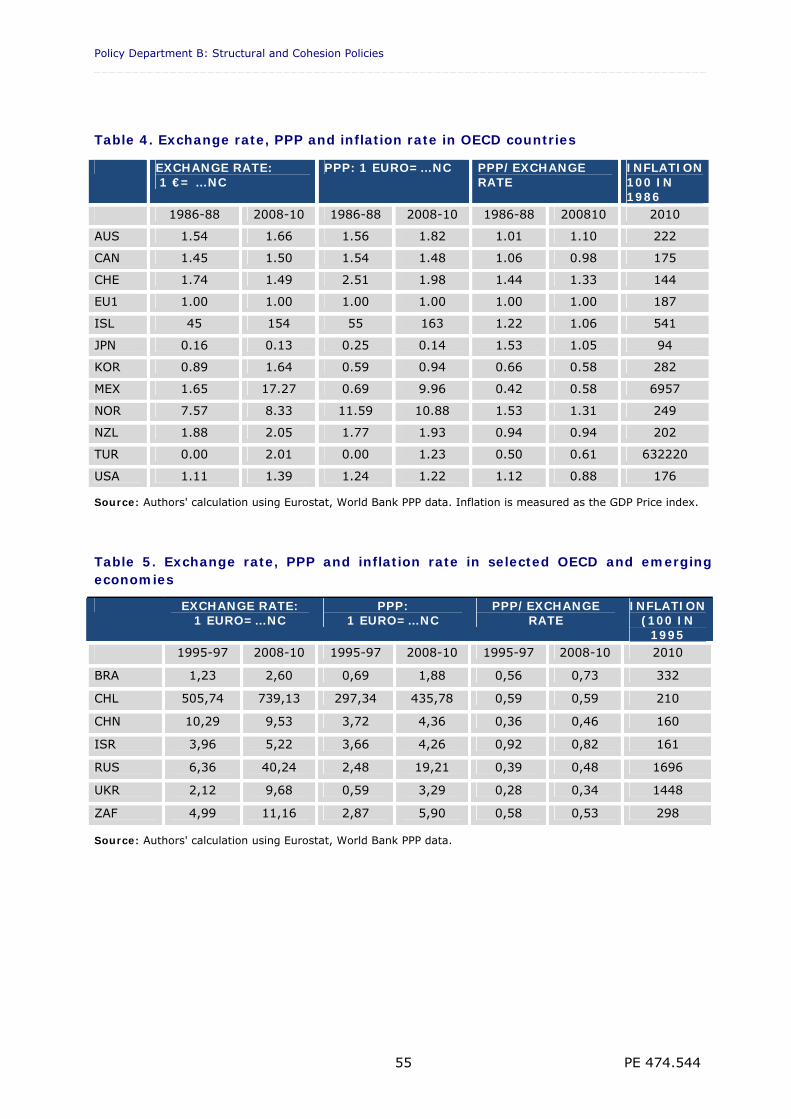
Policy Department B: Structural and Cohesion Policies _________________________________________________________________________________
PE 474.544 55
Table 4. Exchange rate, PPP and inflation rate in OECD countries
EXCHANGE RATE: 1 €= …NC
PPP: 1 EURO=…NC PPP/EXCHANGE RATE
INFLATION 100 IN 1986
1986-88 2008-10 1986-88 2008-10 1986-88 200810 2010
AUS 1.54 1.66 1.56 1.82 1.01 1.10 222
CAN 1.45 1.50 1.54 1.48 1.06 0.98 175
CHE 1.74 1.49 2.51 1.98 1.44 1.33 144
EU1 1.00 1.00 1.00 1.00 1.00 1.00 187
ISL 45 154 55 163 1.22 1.06 541
JPN 0.16 0.13 0.25 0.14 1.53 1.05 94
KOR 0.89 1.64 0.59 0.94 0.66 0.58 282
MEX 1.65 17.27 0.69 9.96 0.42 0.58 6957
NOR 7.57 8.33 11.59 10.88 1.53 1.31 249
NZL 1.88 2.05 1.77 1.93 0.94 0.94 202
TUR 0.00 2.01 0.00 1.23 0.50 0.61 632220
USA 1.11 1.39 1.24 1.22 1.12 0.88 176
Source: Authors' calculation using Eurostat, World Bank PPP data. Inflation is measured as the GDP Price index.
Table 5. Exchange rate, PPP and inflation rate in selected OECD and emerging economies
EXCHANGE RATE: 1 EURO=…NC
PPP: 1 EURO=…NC
PPP/EXCHANGE RATE
INFLATION (100 IN
1995 1995-97 2008-10 1995-97 2008-10 1995-97 2008-10 2010
BRA 1,23 2,60 0,69 1,88 0,56 0,73 332
CHL 505,74 739,13 297,34 435,78 0,59 0,59 210
CHN 10,29 9,53 3,72 4,36 0,36 0,46 160
ISR 3,96 5,22 3,66 4,26 0,92 0,82 161
RUS 6,36 40,24 2,48 19,21 0,39 0,48 1696
UKR 2,12 9,68 0,59 3,29 0,28 0,34 1448
ZAF 4,99 11,16 2,87 5,90 0,58 0,53 298
Source: Authors' calculation using Eurostat, World Bank PPP data.
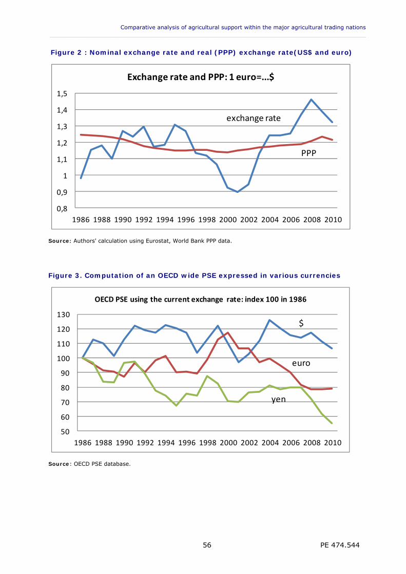
Comparative analysis of agricultural support within the major agricultural trading nations ___________________________________________________________________________________________
PE 474.544 56
Figure 2 : Nominal exchange rate and real (PPP) exchange rate(US$ and euro)
0,8
0,9
1
1,1
1,2
1,3
1,4
1,5
1986 1988 1990 1992 1994 1996 1998 2000 2002 2004 2006 2008 2010
Exchange rate and PPP: 1 euro=...$
PPP
exchange rate
Source: Authors' calculation using Eurostat, World Bank PPP data.
Figure 3. Computation of an OECD wide PSE expressed in various currencies
50
60
70
80
90
100
110
120
130
1986 1988 1990 1992 1994 1996 1998 2000 2002 2004 2006 2008 2010
OECD PSE using the current exchange rate: index 100 in 1986
$
euro
yen
Source: OECD PSE database.
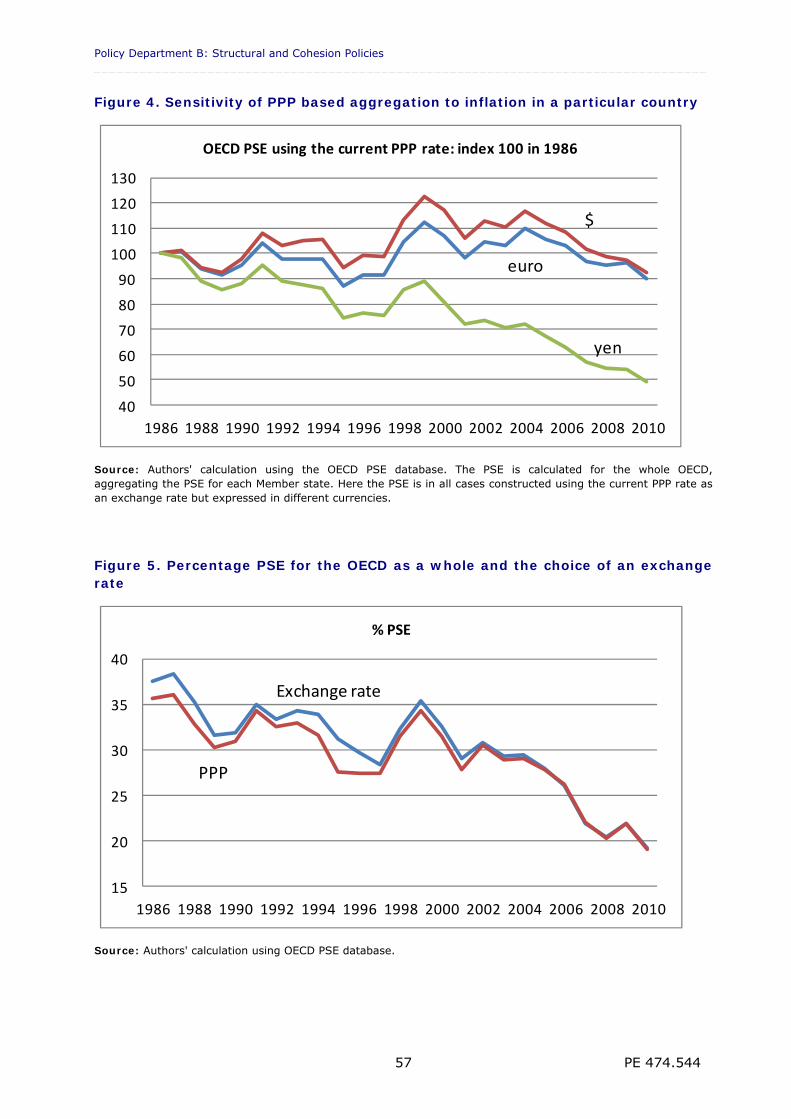
Policy Department B: Structural and Cohesion Policies _________________________________________________________________________________
PE 474.544 57
Figure 4. Sensitivity of PPP based aggregation to inflation in a particular country
40
50
60
70
80
90
100
110
120
130
1986 1988 1990 1992 1994 1996 1998 2000 2002 2004 2006 2008 2010
OECD PSE using the current PPP rate: index 100 in 1986
$
euro
yen
Source: Authors' calculation using the OECD PSE database. The PSE is calculated for the whole OECD, aggregating the PSE for each Member state. Here the PSE is in all cases constructed using the current PPP rate as an exchange rate but expressed in different currencies.
Figure 5. Percentage PSE for the OECD as a whole and the choice of an exchange rate
15
20
25
30
35
40
1986 1988 1990 1992 1994 1996 1998 2000 2002 2004 2006 2008 2010
% PSE
Exchange rate
PPP
Source: Authors' calculation using OECD PSE database.
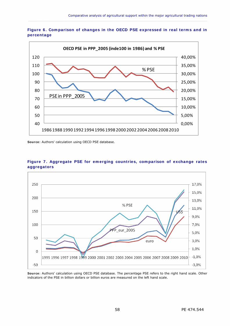
Comparative analysis of agricultural support within the major agricultural trading nations ___________________________________________________________________________________________
PE 474.544 58
Figure 6. Comparison of changes in the OECD PSE expressed in real terms and in percentage
0,00%
5,00%
10,00%
15,00%
20,00%
25,00%
30,00%
35,00%
40,00%
40
50
60
70
80
90
100
110
120
1986198819901992199419961998200020022004200620082010
OECD PSE in PPP_2005 (inde100 in 1986) and % PSE
PSE in PPP_2005
% PSE
Source: Authors' calculation using OECD PSE database.
Figure 7. Aggregate PSE for emerging countries, comparison of exchange rates aggregators
Source: Authors' calculation using OECD PSE database. The percentage PSE refers to the right hand scale. Other indicators of the PSE in billion dollars or billion euros are measured on the left hand scale.
Policy Department B: Structural and Cohesion Policies _________________________________________________________________________________
PE 474.544 59
2.6. Conclusion: the methodology adopted
2.6.1. The methodology
In the following section we will use mostly OECD data. For the analysis of the composition of support we will also use microeconomic and budget data, in particular for the EU, but given the caveats of the WTO notifications, the OECD dataset is the only one that makes it possible to make meaningful comparisons. Because we consider that any measure ignoring the transfers from consumers introduces considerable bias in international comparisons (as well as in intertemporal comparisons in countries where budgetary support has replaced transfers from consumers), we consider the PSE methodology to be currently the most meaningful approach. However, the approach adopted in the next sections departs from the standard OECD methodology in several respects. We develop indicators using a fixed reference PPP as a cross section price index (constructed as an EKS index), which we extrapolate over time using country-specific Fisher indexes of inflation based on GDP. This reduces sensitivity to exogenous factors such as the current under/over valuation of currencies or nominal exchange rates and inflation. Using real measures (PPPs) allows the analysis to unravel price and volume effects, and to control for the effect of exogenous price changes and currency appreciation/depreciation on indicators such as the PSE. Rather than using the complex classification of the OECD which relies on the way support is granted to producers, we use a classification of payments that focuses more on the distorting/non distorting aspect of the payments. For example, the OECD methodology has difficulties in distinguishing countercyclical payments from more production neutral payments, while we believe that it is important to do so. Reference to the WTO classification of payments (Amber vs. Green box) appears relevant here. In particular we explicitly distinguish the role of the coupled support through prices by using a synthetic index of domestic prices relative to border prices. And we isolate the payments that are linked to market conditions, since the OECD methodology tends to give a misleading image of the support in countries which have maintained countercyclical payments. The corresponding budgets might be low during the recent years, but the instrument is in place and the support potential under alternative market conditions should not be underestimated. In terms of transparency and communication, the OECD methodology is too complex to be easily understandable. While the information contained in Appendix 1.2. (OECD labels) is very useful information for an ad hoc classification of payments, for international comparisons we use a simple criterion, which is the ranking of the top payments for each country. We believe that by simplifying information we make it more easily accessible.
2.6.2. The list of countries to focus on
In order to assess how EU agricultural support compared to other major trading nations, we selected a sample of countries on a rather ad hoc basis. The goal is to focus both on major trading partners and on countries that show particular forms of support whose relevance is currently discussed in the EU.
Comparative analysis of agricultural support within the major agricultural trading nations ___________________________________________________________________________________________
PE 474.544 60
In Section 3 we provide a comparison of the measures of support based on the indicator defined in the previous section. We rely on the OECD data even though our calculations require using other sources of information for the PPPs (namely Eurostat and the World Bank) in order to express support in real values. Because we rely on a consistent dataset, we are able to consider the EU, Australia, Canada, Switzerland, Iceland, Japan, Korea, Mexico, Norway, New Zealand, Turkey, USA and some emerging economies, i.e., Brazil, Chile, People's Republic of China, Israel, the Russian Federation, Ukraine and the South African Republic (note that Chile and Israel are OECD members). We detail how the various instruments differ between the EU (Section 4) and other typical countries (Section 5). The case of the US is interesting since, while the level of support is lower than in the EU, the US has maintained a system of payments that tends to protect farmers from both price and output fluctuations. The case of Canada is also illustrative, since historically Canada has supported farmers in indirect ways, such as subsidising the transportation of grains, and has recently developed instruments to protect farmers from market fluctuations. Switzerland, while not being a major trading partner, has developed forms of support that focus on specific public goods, such as the protection of rural vitality, biodiversity, and landscapes, all of which are of considerable interest for the definition of the future CAP in the EU. Finally, China and Brazil are of particular interest, since they tend to support infrastructure and the modernization of the sector rather than supporting farm incomes as the EU does.
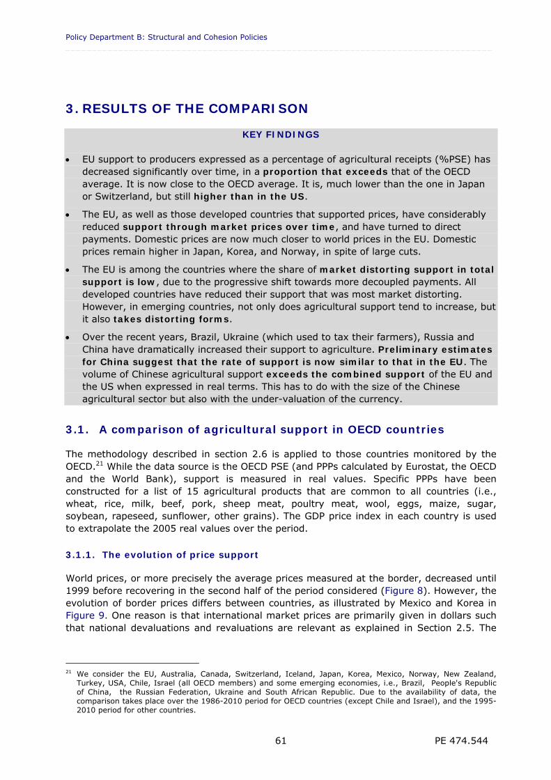
Policy Department B: Structural and Cohesion Policies _________________________________________________________________________________
PE 474.544 61
3. RESULTS OF THE COMPARISON
KEY FINDINGS EU support to producers expressed as a percentage of agricultural receipts (%PSE) has
decreased significantly over time, in a proportion that exceeds that of the OECD average. It is now close to the OECD average. It is, much lower than the one in Japan or Switzerland, but still higher than in the US.
The EU, as well as those developed countries that supported prices, have considerably reduced support through market prices over time, and have turned to direct payments. Domestic prices are now much closer to world prices in the EU. Domestic prices remain higher in Japan, Korea, and Norway, in spite of large cuts.
The EU is among the countries where the share of market distorting support in total support is low, due to the progressive shift towards more decoupled payments. All developed countries have reduced their support that was most market distorting. However, in emerging countries, not only does agricultural support tend to increase, but it also takes distorting forms.
Over the recent years, Brazil, Ukraine (which used to tax their farmers), Russia and China have dramatically increased their support to agriculture. Preliminary estimates for China suggest that the rate of support is now similar to that in the EU. The volume of Chinese agricultural support exceeds the combined support of the EU and the US when expressed in real terms. This has to do with the size of the Chinese agricultural sector but also with the under-valuation of the currency.
3.1. A comparison of agricultural support in OECD countries
The methodology described in section 2.6 is applied to those countries monitored by the OECD.21 While the data source is the OECD PSE (and PPPs calculated by Eurostat, the OECD and the World Bank), support is measured in real values. Specific PPPs have been constructed for a list of 15 agricultural products that are common to all countries (i.e., wheat, rice, milk, beef, pork, sheep meat, poultry meat, wool, eggs, maize, sugar, soybean, rapeseed, sunflower, other grains). The GDP price index in each country is used to extrapolate the 2005 real values over the period.
3.1.1. The evolution of price support
World prices, or more precisely the average prices measured at the border, decreased until 1999 before recovering in the second half of the period considered (Figure 8). However, the evolution of border prices differs between countries, as illustrated by Mexico and Korea in Figure 9. One reason is that international market prices are primarily given in dollars such that national devaluations and revaluations are relevant as explained in Section 2.5. The
21 We consider the EU, Australia, Canada, Switzerland, Iceland, Japan, Korea, Mexico, Norway, New Zealand,
Turkey, USA, Chile, Israel (all OECD members) and some emerging economies, i.e., Brazil, People's Republic of China, the Russian Federation, Ukraine and South African Republic. Due to the availability of data, the comparison takes place over the 1986-2010 period for OECD countries (except Chile and Israel), and the 1995-2010 period for other countries.
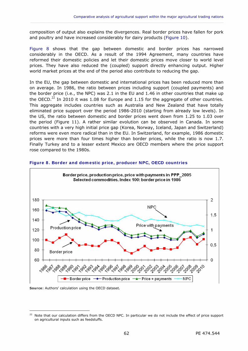
Comparative analysis of agricultural support within the major agricultural trading nations ___________________________________________________________________________________________
PE 474.544 62
composition of output also explains the divergences. Real border prices have fallen for pork and poultry and have increased considerably for dairy products (Figure 10). Figure 8 shows that the gap between domestic and border prices has narrowed considerably in the OECD. As a result of the 1994 Agreement, many countries have reformed their domestic policies and let their domestic prices move closer to world level prices. They have also reduced the (coupled) support directly enhancing output. Higher world market prices at the end of the period also contribute to reducing the gap. In the EU, the gap between domestic and international prices has been reduced more than on average. In 1986, the ratio between prices including support (coupled payments) and the border price (i.e., the NPC) was 2.1 in the EU and 1.46 in other countries that make up the OECD.22 In 2010 it was 1.08 for Europe and 1.15 for the aggregate of other countries. This aggregate includes countries such as Australia and New Zealand that have totally eliminated price support over the period 1986-2010 (starting from already low levels). In the US, the ratio between domestic and border prices went down from 1.25 to 1.03 over the period (Figure 11). A rather similar evolution can be observed in Canada. In some countries with a very high initial price gap (Korea, Norway, Iceland, Japan and Switzerland) reforms were even more radical than in the EU. In Switzerland, for example, 1986 domestic prices were more than four times higher than border prices, while the ratio is now 1.7. Finally Turkey and to a lesser extent Mexico are OECD members where the price support rose compared to the 1980s.
Figure 8. Border and domestic price, producer NPC, OECD countries
Source: Authors' calculation using the OECD dataset.
22 Note that our calculation differs from the OECD NPC. In particular we do not include the effect of price support
on agricultural inputs such as feedstuffs.
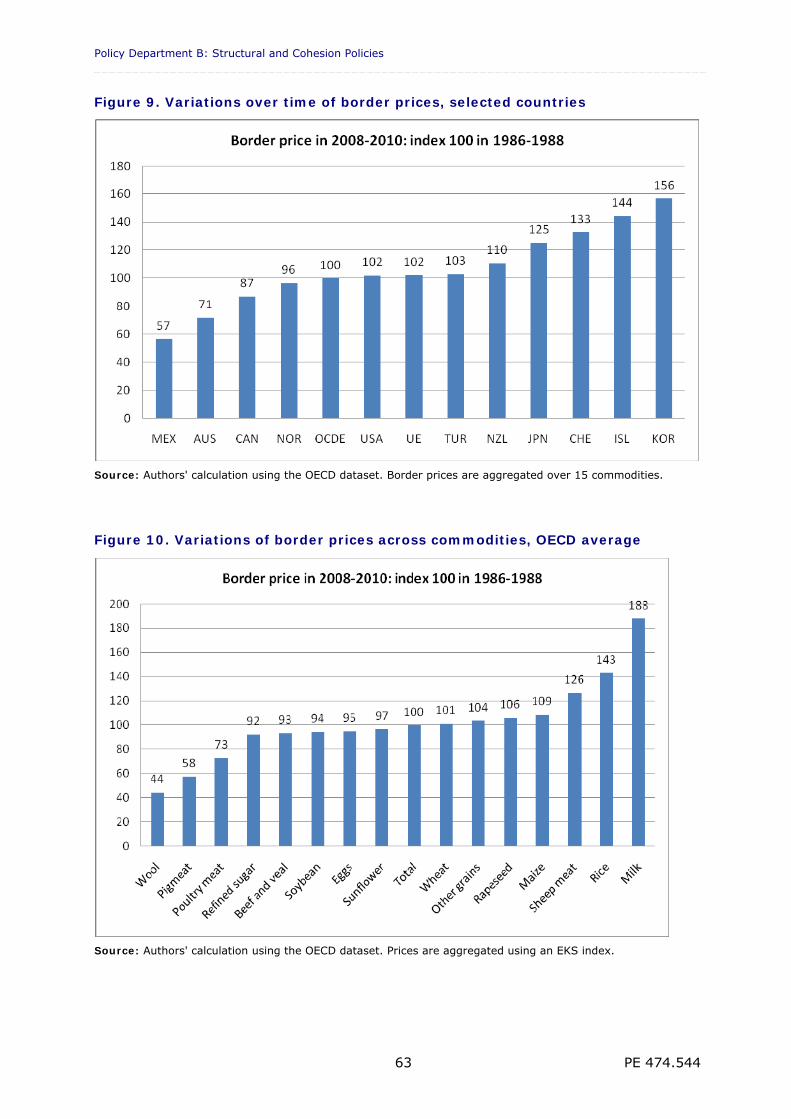
Policy Department B: Structural and Cohesion Policies _________________________________________________________________________________
PE 474.544 63
Figure 9. Variations over time of border prices, selected countries
Source: Authors' calculation using the OECD dataset. Border prices are aggregated over 15 commodities.
Figure 10. Variations of border prices across commodities, OECD average
Source: Authors' calculation using the OECD dataset. Prices are aggregated using an EKS index.
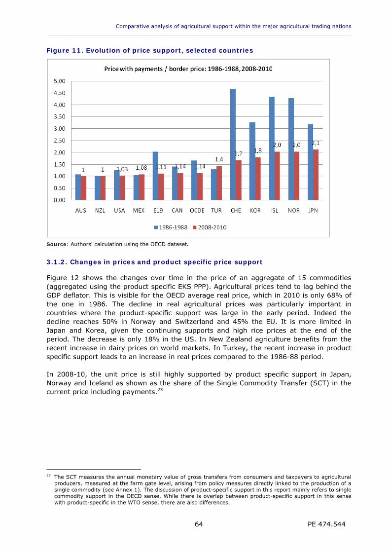
Comparative analysis of agricultural support within the major agricultural trading nations ___________________________________________________________________________________________
PE 474.544 64
Figure 11. Evolution of price support, selected countries
Source: Authors' calculation using the OECD dataset.
3.1.2. Changes in prices and product specific price support
Figure 12 shows the changes over time in the price of an aggregate of 15 commodities (aggregated using the product specific EKS PPP). Agricultural prices tend to lag behind the GDP deflator. This is visible for the OECD average real price, which in 2010 is only 68% of the one in 1986. The decline in real agricultural prices was particularly important in countries where the product-specific support was large in the early period. Indeed the decline reaches 50% in Norway and Switzerland and 45% the EU. It is more limited in Japan and Korea, given the continuing supports and high rice prices at the end of the period. The decrease is only 18% in the US. In New Zealand agriculture benefits from the recent increase in dairy prices on world markets. In Turkey, the recent increase in product specific support leads to an increase in real prices compared to the 1986-88 period. In 2008-10, the unit price is still highly supported by product specific support in Japan, Norway and Iceland as shown as the share of the Single Commodity Transfer (SCT) in the current price including payments.23
23 The SCT measures the annual monetary value of gross transfers from consumers and taxpayers to agricultural
producers, measured at the farm gate level, arising from policy measures directly linked to the production of a single commodity (see Annex 1). The discussion of product-specific support in this report mainly refers to single commodity support in the OECD sense. While there is overlap between product-specific support in this sense with product-specific in the WTO sense, there are also differences.
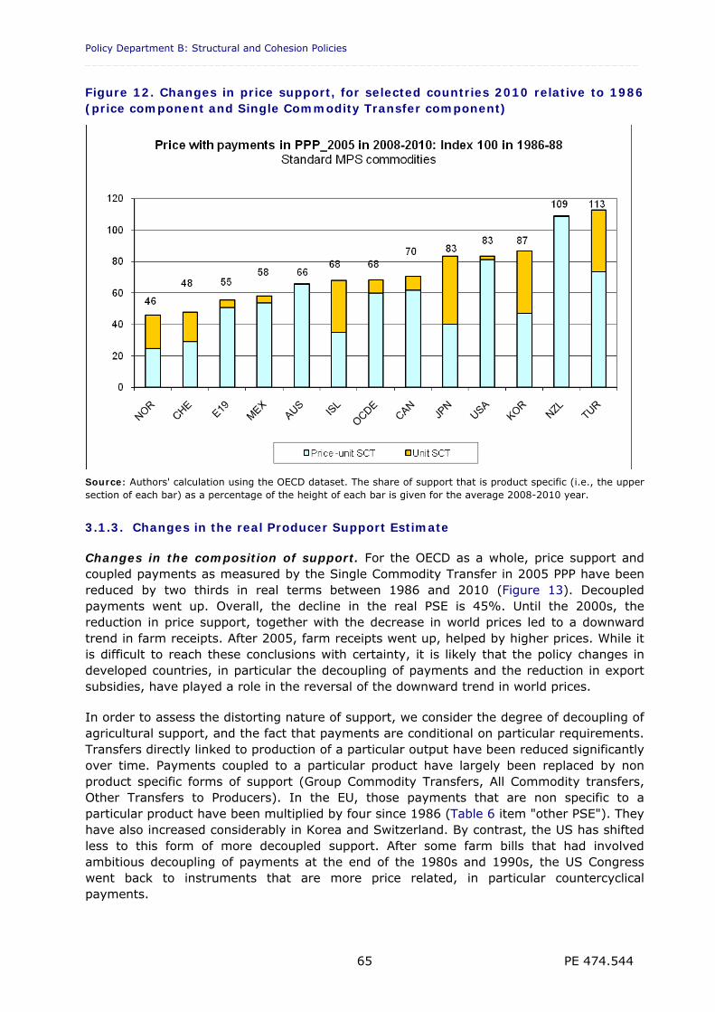
Policy Department B: Structural and Cohesion Policies _________________________________________________________________________________
PE 474.544 65
Figure 12. Changes in price support, for selected countries 2010 relative to 1986 (price component and Single Commodity Transfer component)
Source: Authors' calculation using the OECD dataset. The share of support that is product specific (i.e., the upper section of each bar) as a percentage of the height of each bar is given for the average 2008-2010 year.
3.1.3. Changes in the real Producer Support Estimate
Changes in the composition of support. For the OECD as a whole, price support and coupled payments as measured by the Single Commodity Transfer in 2005 PPP have been reduced by two thirds in real terms between 1986 and 2010 (Figure 13). Decoupled payments went up. Overall, the decline in the real PSE is 45%. Until the 2000s, the reduction in price support, together with the decrease in world prices led to a downward trend in farm receipts. After 2005, farm receipts went up, helped by higher prices. While it is difficult to reach these conclusions with certainty, it is likely that the policy changes in developed countries, in particular the decoupling of payments and the reduction in export subsidies, have played a role in the reversal of the downward trend in world prices. In order to assess the distorting nature of support, we consider the degree of decoupling of agricultural support, and the fact that payments are conditional on particular requirements. Transfers directly linked to production of a particular output have been reduced significantly over time. Payments coupled to a particular product have largely been replaced by non product specific forms of support (Group Commodity Transfers, All Commodity transfers, Other Transfers to Producers). In the EU, those payments that are non specific to a particular product have been multiplied by four since 1986 (Table 6 item "other PSE"). They have also increased considerably in Korea and Switzerland. By contrast, the US has shifted less to this form of more decoupled support. After some farm bills that had involved ambitious decoupling of payments at the end of the 1980s and 1990s, the US Congress went back to instruments that are more price related, in particular countercyclical payments.
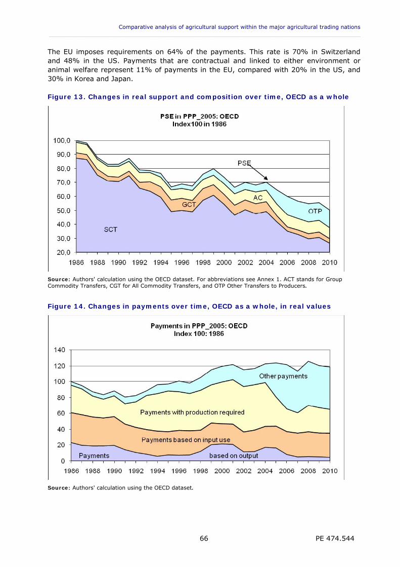
Comparative analysis of agricultural support within the major agricultural trading nations ___________________________________________________________________________________________
PE 474.544 66
The EU imposes requirements on 64% of the payments. This rate is 70% in Switzerland and 48% in the US. Payments that are contractual and linked to either environment or animal welfare represent 11% of payments in the EU, compared with 20% in the US, and 30% in Korea and Japan. Figure 13. Changes in real support and composition over time, OECD as a whole
Source: Authors' calculation using the OECD dataset. For abbreviations see Annex 1. ACT stands for Group Commodity Transfers, CGT for All Commodity Transfers, and OTP Other Transfers to Producers.
Figure 14. Changes in payments over time, OECD as a whole, in real values
Source: Authors' calculation using the OECD dataset.
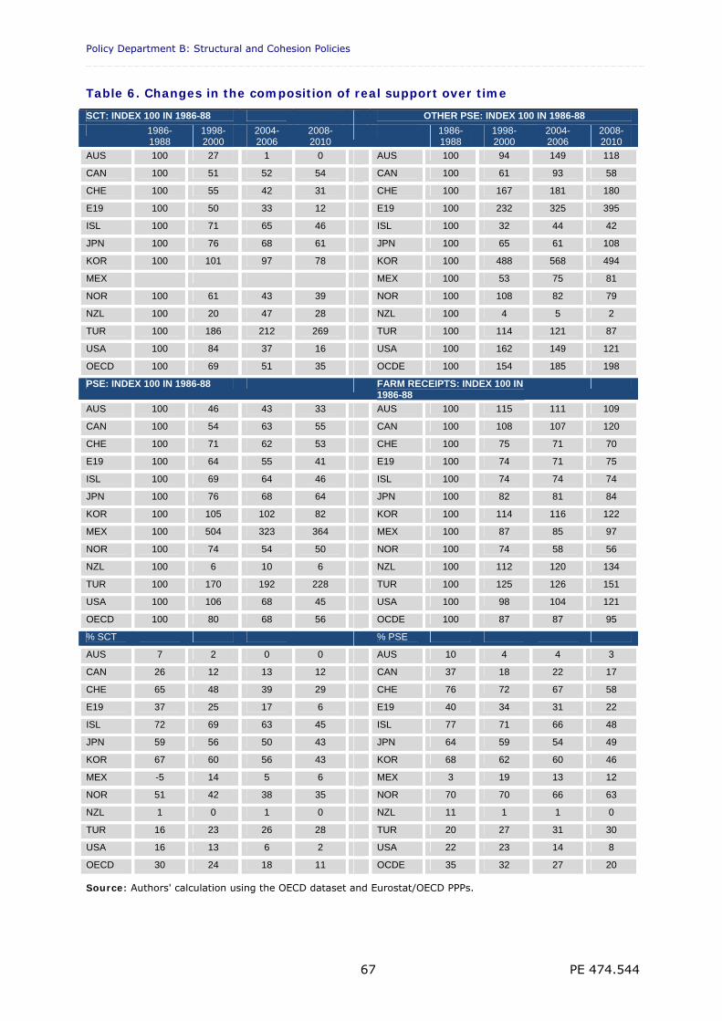
Policy Department B: Structural and Cohesion Policies _________________________________________________________________________________
PE 474.544 67
Table 6. Changes in the composition of real support over time
SCT: INDEX 100 IN 1986-88 OTHER PSE: INDEX 100 IN 1986-88 1986-
1988 1998-2000
2004-2006
2008-2010
1986-1988
1998-2000
2004-2006
2008-2010
AUS 100 27 1 0 AUS 100 94 149 118
CAN 100 51 52 54 CAN 100 61 93 58
CHE 100 55 42 31 CHE 100 167 181 180
E19 100 50 33 12 E19 100 232 325 395
ISL 100 71 65 46 ISL 100 32 44 42
JPN 100 76 68 61 JPN 100 65 61 108
KOR 100 101 97 78 KOR 100 488 568 494
MEX MEX 100 53 75 81
NOR 100 61 43 39 NOR 100 108 82 79
NZL 100 20 47 28 NZL 100 4 5 2
TUR 100 186 212 269 TUR 100 114 121 87
USA 100 84 37 16 USA 100 162 149 121
OECD 100 69 51 35 OCDE 100 154 185 198
PSE: INDEX 100 IN 1986-88 FARM RECEIPTS: INDEX 100 IN 1986-88
AUS 100 46 43 33 AUS 100 115 111 109
CAN 100 54 63 55 CAN 100 108 107 120
CHE 100 71 62 53 CHE 100 75 71 70
E19 100 64 55 41 E19 100 74 71 75
ISL 100 69 64 46 ISL 100 74 74 74
JPN 100 76 68 64 JPN 100 82 81 84
KOR 100 105 102 82 KOR 100 114 116 122
MEX 100 504 323 364 MEX 100 87 85 97
NOR 100 74 54 50 NOR 100 74 58 56
NZL 100 6 10 6 NZL 100 112 120 134
TUR 100 170 192 228 TUR 100 125 126 151
USA 100 106 68 45 USA 100 98 104 121
OECD 100 80 68 56 OCDE 100 87 87 95
% SCT % PSE
AUS 7 2 0 0 AUS 10 4 4 3
CAN 26 12 13 12 CAN 37 18 22 17
CHE 65 48 39 29 CHE 76 72 67 58
E19 37 25 17 6 E19 40 34 31 22
ISL 72 69 63 45 ISL 77 71 66 48
JPN 59 56 50 43 JPN 64 59 54 49
KOR 67 60 56 43 KOR 68 62 60 46
MEX -5 14 5 6 MEX 3 19 13 12
NOR 51 42 38 35 NOR 70 70 66 63
NZL 1 0 1 0 NZL 11 1 1 0
TUR 16 23 26 28 TUR 20 27 31 30
USA 16 13 6 2 USA 22 23 14 8
OECD 30 24 18 11 OCDE 35 32 27 20
Source: Authors' calculation using the OECD dataset and Eurostat/OECD PPPs.
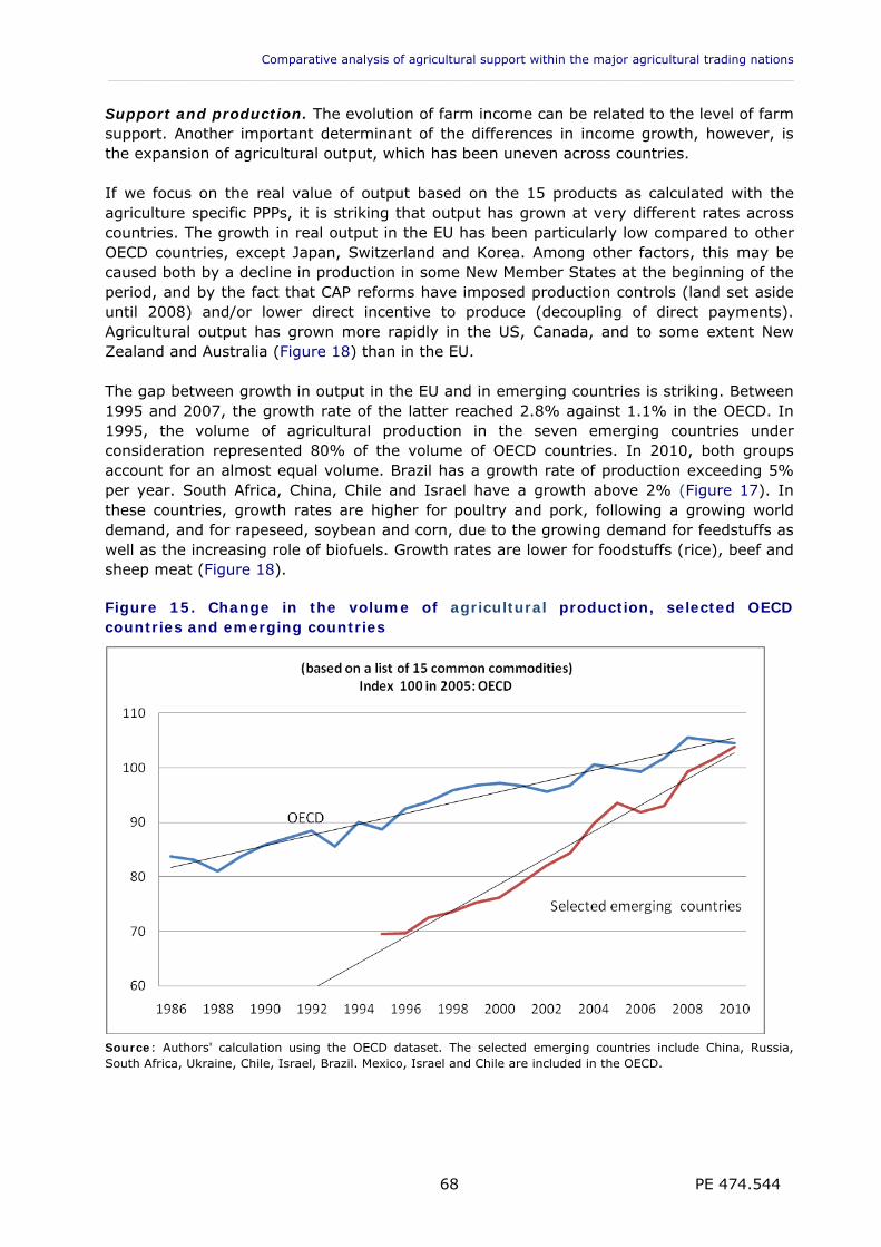
Comparative analysis of agricultural support within the major agricultural trading nations ___________________________________________________________________________________________
PE 474.544 68
Support and production. The evolution of farm income can be related to the level of farm support. Another important determinant of the differences in income growth, however, is the expansion of agricultural output, which has been uneven across countries. If we focus on the real value of output based on the 15 products as calculated with the agriculture specific PPPs, it is striking that output has grown at very different rates across countries. The growth in real output in the EU has been particularly low compared to other OECD countries, except Japan, Switzerland and Korea. Among other factors, this may be caused both by a decline in production in some New Member States at the beginning of the period, and by the fact that CAP reforms have imposed production controls (land set aside until 2008) and/or lower direct incentive to produce (decoupling of direct payments). Agricultural output has grown more rapidly in the US, Canada, and to some extent New Zealand and Australia (Figure 18) than in the EU. The gap between growth in output in the EU and in emerging countries is striking. Between 1995 and 2007, the growth rate of the latter reached 2.8% against 1.1% in the OECD. In 1995, the volume of agricultural production in the seven emerging countries under consideration represented 80% of the volume of OECD countries. In 2010, both groups account for an almost equal volume. Brazil has a growth rate of production exceeding 5% per year. South Africa, China, Chile and Israel have a growth above 2% (Figure 17). In these countries, growth rates are higher for poultry and pork, following a growing world demand, and for rapeseed, soybean and corn, due to the growing demand for feedstuffs as well as the increasing role of biofuels. Growth rates are lower for foodstuffs (rice), beef and sheep meat (Figure 18). Figure 15. Change in the volume of agricultural production, selected OECD countries and emerging countries
Source: Authors' calculation using the OECD dataset. The selected emerging countries include China, Russia, South Africa, Ukraine, Chile, Israel, Brazil. Mexico, Israel and Chile are included in the OECD.
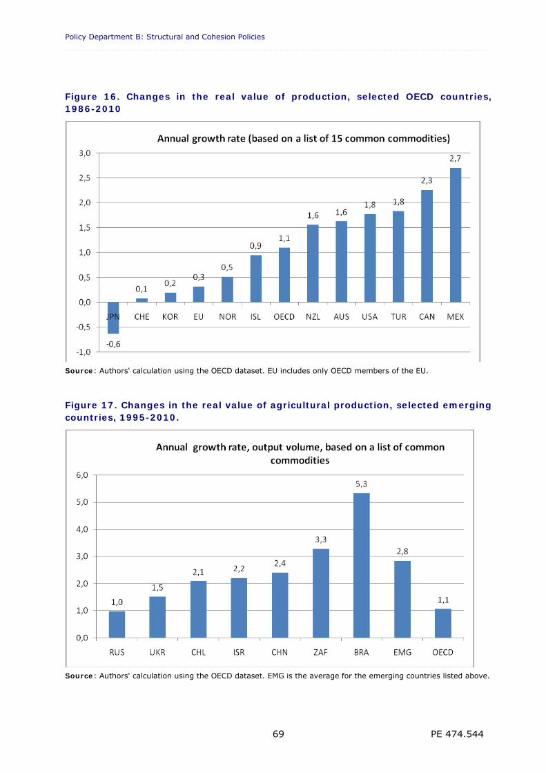
Policy Department B: Structural and Cohesion Policies _________________________________________________________________________________
PE 474.544 69
Figure 16. Changes in the real value of production, selected OECD countries, 1986-2010
Source: Authors' calculation using the OECD dataset. EU includes only OECD members of the EU.
Figure 17. Changes in the real value of agricultural production, selected emerging countries, 1995-2010.
Source: Authors' calculation using the OECD dataset. EMG is the average for the emerging countries listed above.
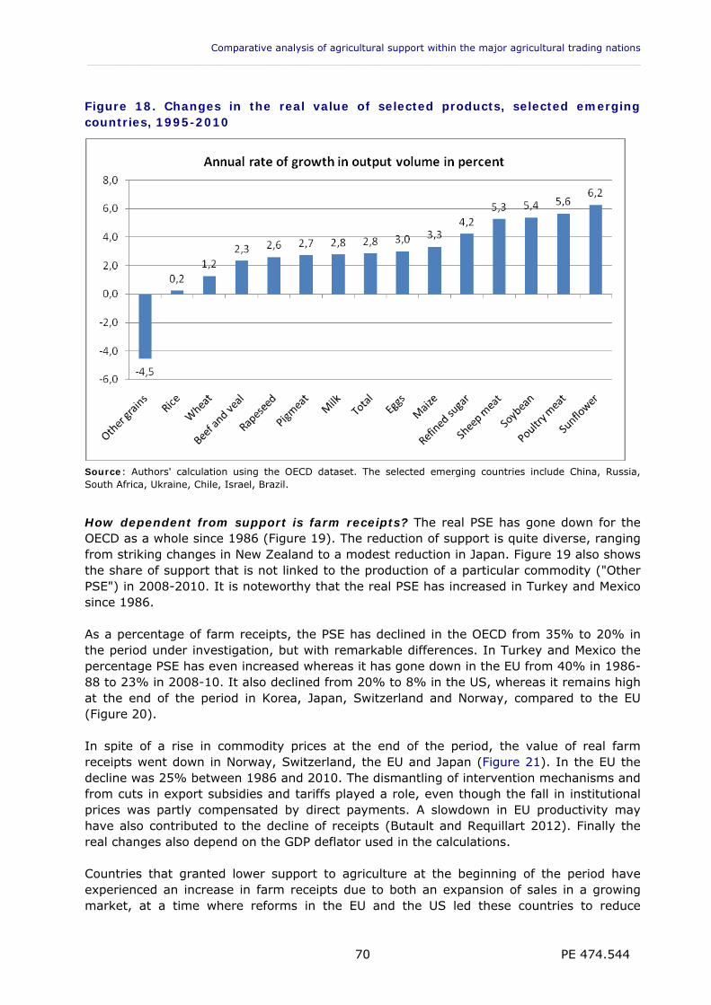
Comparative analysis of agricultural support within the major agricultural trading nations ___________________________________________________________________________________________
PE 474.544 70
Figure 18. Changes in the real value of selected products, selected emerging countries, 1995-2010
Source: Authors' calculation using the OECD dataset. The selected emerging countries include China, Russia, South Africa, Ukraine, Chile, Israel, Brazil.
How dependent from support is farm receipts? The real PSE has gone down for the OECD as a whole since 1986 (Figure 19). The reduction of support is quite diverse, ranging from striking changes in New Zealand to a modest reduction in Japan. Figure 19 also shows the share of support that is not linked to the production of a particular commodity ("Other PSE") in 2008-2010. It is noteworthy that the real PSE has increased in Turkey and Mexico since 1986. As a percentage of farm receipts, the PSE has declined in the OECD from 35% to 20% in the period under investigation, but with remarkable differences. In Turkey and Mexico the percentage PSE has even increased whereas it has gone down in the EU from 40% in 1986-88 to 23% in 2008-10. It also declined from 20% to 8% in the US, whereas it remains high at the end of the period in Korea, Japan, Switzerland and Norway, compared to the EU (Figure 20). In spite of a rise in commodity prices at the end of the period, the value of real farm receipts went down in Norway, Switzerland, the EU and Japan (Figure 21). In the EU the decline was 25% between 1986 and 2010. The dismantling of intervention mechanisms and from cuts in export subsidies and tariffs played a role, even though the fall in institutional prices was partly compensated by direct payments. A slowdown in EU productivity may have also contributed to the decline of receipts (Butault and Requillart 2012). Finally the real changes also depend on the GDP deflator used in the calculations. Countries that granted lower support to agriculture at the beginning of the period have experienced an increase in farm receipts due to both an expansion of sales in a growing market, at a time where reforms in the EU and the US led these countries to reduce

Policy Department B: Structural and Cohesion Policies _________________________________________________________________________________
PE 474.544 71
exports, and the positive trend in world market prices at the end of the period. Over the period, real farm receipts grew by 34% in New Zealand, for example, in sharp contrast with the EU (which also benefited less from the boom on dairy markets than New Zealand). The EU has managed most of the adjustment to market conditions. There is little scope for further decrease in coupled support in the future. In case of high world prices, producers will be able to take advantage of them, while this might not be the case in Korea and Norway, where domestic prices are still higher than world prices and where reforms have not gone as far as in the EU. Figure 19. Changes over time and composition of real support (in 2008-2010), selected countries
Source: Authors' calculation using the OECD dataset.
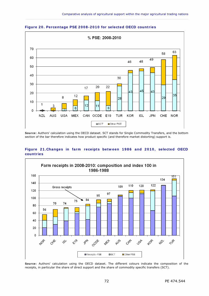
Comparative analysis of agricultural support within the major agricultural trading nations ___________________________________________________________________________________________
PE 474.544 72
Figure 20. Percentage PSE 2008-2010 for selected OECD countries
Source: Authors' calculation using the OECD dataset. SCT stands for Single Commodity Transfers, and the bottom section of the bar therefore indicates how product specific (and therefore market distorting) support is.
Figure 21.Changes in farm receipts between 1986 and 2010, selected OECD countries
Source: Authors' calculation using the OECD dataset. The different colours indicate the composition of the receipts, in particular the share of direct support and the share of commodity specific transfers (SCT).
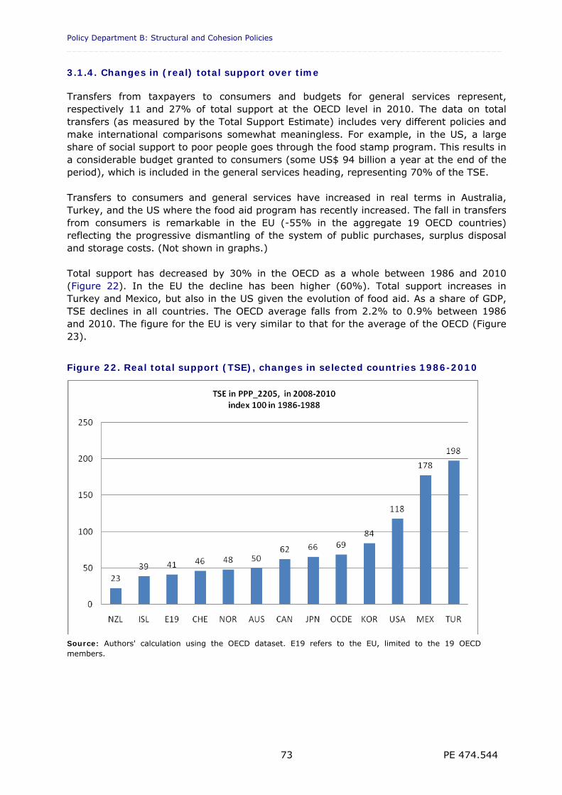
Policy Department B: Structural and Cohesion Policies _________________________________________________________________________________
PE 474.544 73
3.1.4. Changes in (real) total support over time
Transfers from taxpayers to consumers and budgets for general services represent, respectively 11 and 27% of total support at the OECD level in 2010. The data on total transfers (as measured by the Total Support Estimate) includes very different policies and make international comparisons somewhat meaningless. For example, in the US, a large share of social support to poor people goes through the food stamp program. This results in a considerable budget granted to consumers (some US$ 94 billion a year at the end of the period), which is included in the general services heading, representing 70% of the TSE. Transfers to consumers and general services have increased in real terms in Australia, Turkey, and the US where the food aid program has recently increased. The fall in transfers from consumers is remarkable in the EU (-55% in the aggregate 19 OECD countries) reflecting the progressive dismantling of the system of public purchases, surplus disposal and storage costs. (Not shown in graphs.) Total support has decreased by 30% in the OECD as a whole between 1986 and 2010 (Figure 22). In the EU the decline has been higher (60%). Total support increases in Turkey and Mexico, but also in the US given the evolution of food aid. As a share of GDP, TSE declines in all countries. The OECD average falls from 2.2% to 0.9% between 1986 and 2010. The figure for the EU is very similar to that for the average of the OECD (Figure 23).
Figure 22. Real total support (TSE), changes in selected countries 1986-2010
Source: Authors' calculation using the OECD dataset. E19 refers to the EU, limited to the 19 OECD members.
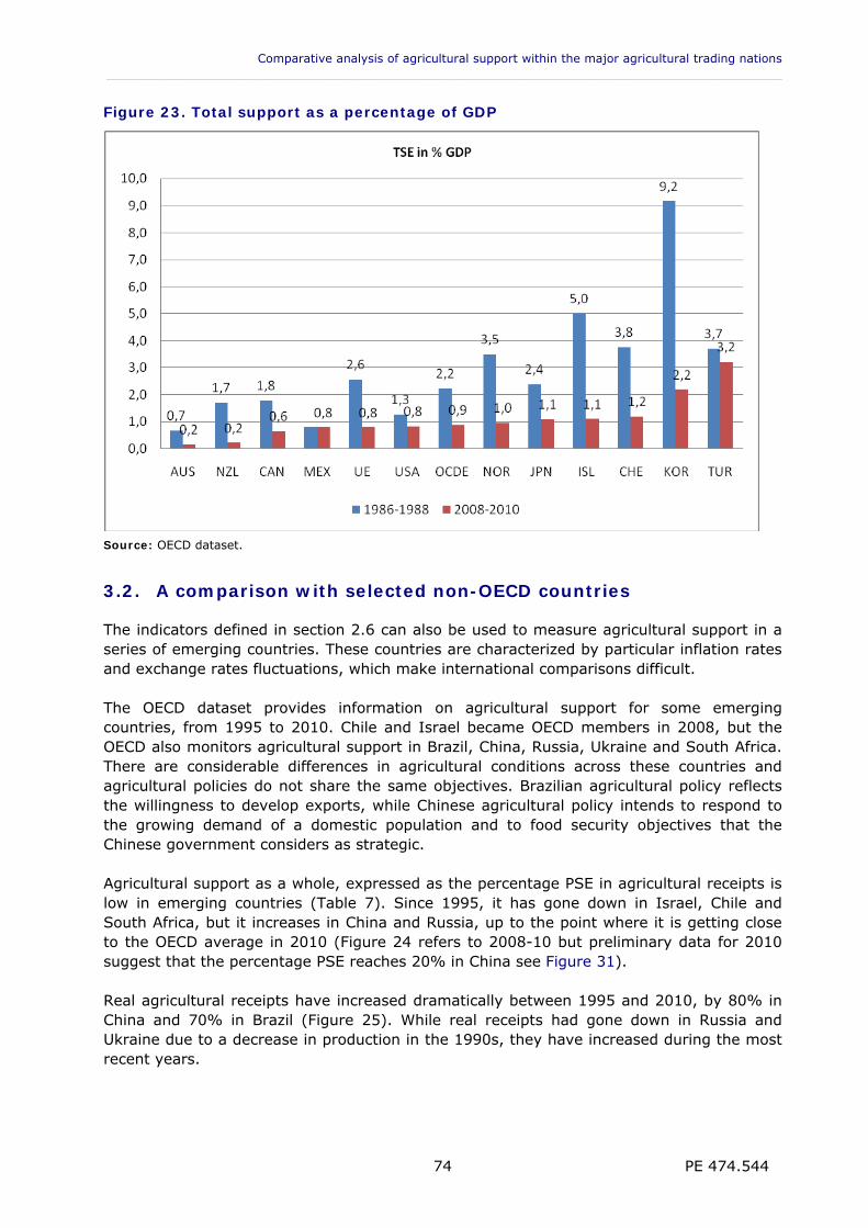
Comparative analysis of agricultural support within the major agricultural trading nations ___________________________________________________________________________________________
PE 474.544 74
Figure 23. Total support as a percentage of GDP
Source: OECD dataset.
3.2. A comparison with selected non-OECD countries
The indicators defined in section 2.6 can also be used to measure agricultural support in a series of emerging countries. These countries are characterized by particular inflation rates and exchange rates fluctuations, which make international comparisons difficult. The OECD dataset provides information on agricultural support for some emerging countries, from 1995 to 2010. Chile and Israel became OECD members in 2008, but the OECD also monitors agricultural support in Brazil, China, Russia, Ukraine and South Africa. There are considerable differences in agricultural conditions across these countries and agricultural policies do not share the same objectives. Brazilian agricultural policy reflects the willingness to develop exports, while Chinese agricultural policy intends to respond to the growing demand of a domestic population and to food security objectives that the Chinese government considers as strategic. Agricultural support as a whole, expressed as the percentage PSE in agricultural receipts is low in emerging countries (Table 7). Since 1995, it has gone down in Israel, Chile and South Africa, but it increases in China and Russia, up to the point where it is getting close to the OECD average in 2010 (Figure 24 refers to 2008-10 but preliminary data for 2010 suggest that the percentage PSE reaches 20% in China see Figure 31). Real agricultural receipts have increased dramatically between 1995 and 2010, by 80% in China and 70% in Brazil (Figure 25). While real receipts had gone down in Russia and Ukraine due to a decrease in production in the 1990s, they have increased during the most recent years.
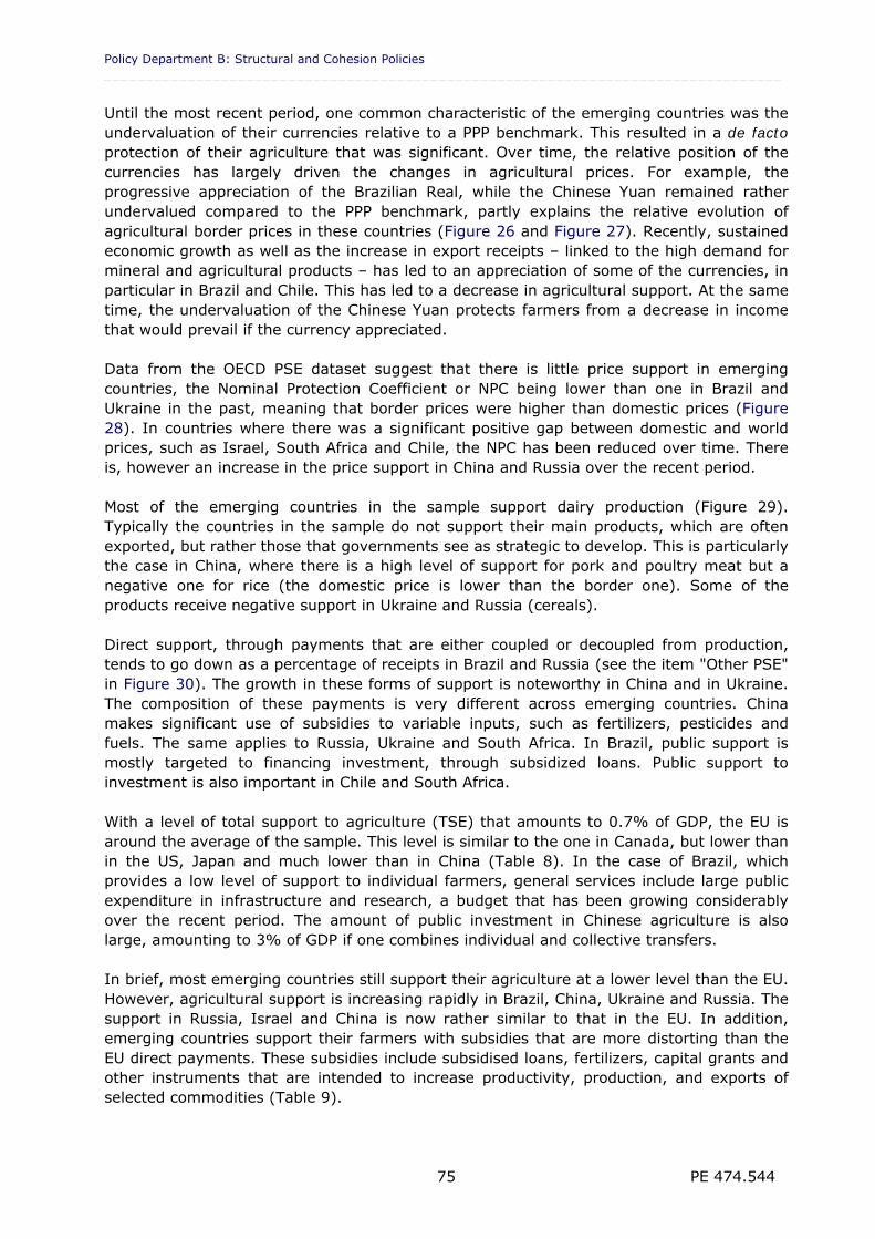
Policy Department B: Structural and Cohesion Policies _________________________________________________________________________________
PE 474.544 75
Until the most recent period, one common characteristic of the emerging countries was the undervaluation of their currencies relative to a PPP benchmark. This resulted in a de facto protection of their agriculture that was significant. Over time, the relative position of the currencies has largely driven the changes in agricultural prices. For example, the progressive appreciation of the Brazilian Real, while the Chinese Yuan remained rather undervalued compared to the PPP benchmark, partly explains the relative evolution of agricultural border prices in these countries (Figure 26 and Figure 27). Recently, sustained economic growth as well as the increase in export receipts – linked to the high demand for mineral and agricultural products – has led to an appreciation of some of the currencies, in particular in Brazil and Chile. This has led to a decrease in agricultural support. At the same time, the undervaluation of the Chinese Yuan protects farmers from a decrease in income that would prevail if the currency appreciated. Data from the OECD PSE dataset suggest that there is little price support in emerging countries, the Nominal Protection Coefficient or NPC being lower than one in Brazil and Ukraine in the past, meaning that border prices were higher than domestic prices (Figure 28). In countries where there was a significant positive gap between domestic and world prices, such as Israel, South Africa and Chile, the NPC has been reduced over time. There is, however an increase in the price support in China and Russia over the recent period. Most of the emerging countries in the sample support dairy production (Figure 29). Typically the countries in the sample do not support their main products, which are often exported, but rather those that governments see as strategic to develop. This is particularly the case in China, where there is a high level of support for pork and poultry meat but a negative one for rice (the domestic price is lower than the border one). Some of the products receive negative support in Ukraine and Russia (cereals). Direct support, through payments that are either coupled or decoupled from production, tends to go down as a percentage of receipts in Brazil and Russia (see the item "Other PSE" in Figure 30). The growth in these forms of support is noteworthy in China and in Ukraine. The composition of these payments is very different across emerging countries. China makes significant use of subsidies to variable inputs, such as fertilizers, pesticides and fuels. The same applies to Russia, Ukraine and South Africa. In Brazil, public support is mostly targeted to financing investment, through subsidized loans. Public support to investment is also important in Chile and South Africa. With a level of total support to agriculture (TSE) that amounts to 0.7% of GDP, the EU is around the average of the sample. This level is similar to the one in Canada, but lower than in the US, Japan and much lower than in China (Table 8). In the case of Brazil, which provides a low level of support to individual farmers, general services include large public expenditure in infrastructure and research, a budget that has been growing considerably over the recent period. The amount of public investment in Chinese agriculture is also large, amounting to 3% of GDP if one combines individual and collective transfers. In brief, most emerging countries still support their agriculture at a lower level than the EU. However, agricultural support is increasing rapidly in Brazil, China, Ukraine and Russia. The support in Russia, Israel and China is now rather similar to that in the EU. In addition, emerging countries support their farmers with subsidies that are more distorting than the EU direct payments. These subsidies include subsidised loans, fertilizers, capital grants and other instruments that are intended to increase productivity, production, and exports of selected commodities (Table 9).
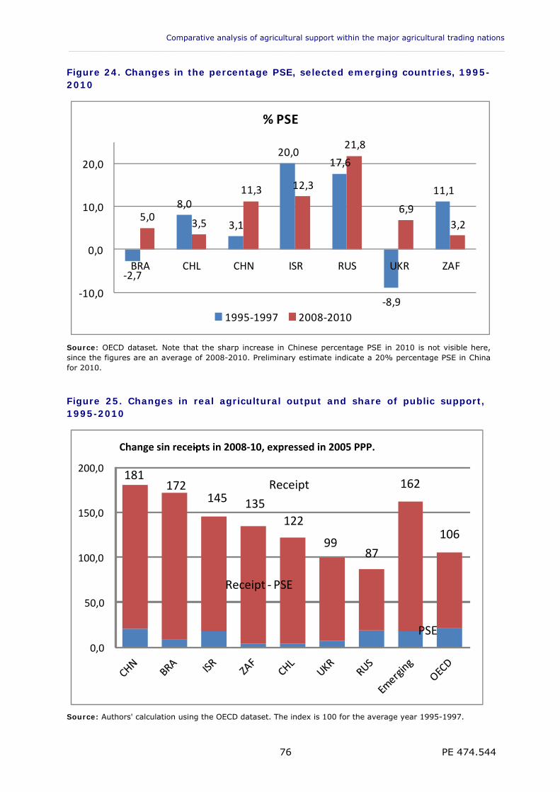
Comparative analysis of agricultural support within the major agricultural trading nations ___________________________________________________________________________________________
PE 474.544 76
Figure 24. Changes in the percentage PSE, selected emerging countries, 1995-2010
‐2,7
8,0
3,1
20,017,6
‐8,9
11,1
5,03,5
11,3 12,3
21,8
6,9
3,2
‐10,0
0,0
10,0
20,0
BRA CHL CHN ISR RUS UKR ZAF
% PSE
1995‐1997 2008‐2010
Source: OECD dataset. Note that the sharp increase in Chinese percentage PSE in 2010 is not visible here, since the figures are an average of 2008-2010. Preliminary estimate indicate a 20% percentage PSE in China for 2010.
Figure 25. Changes in real agricultural output and share of public support, 1995-2010
Source: Authors' calculation using the OECD dataset. The index is 100 for the average year 1995-1997.
0,0
50,0
100,0
150,0
200,0
Change sin receipts in 2008‐10, expressed in 2005 PPP. ‐
PSE
Receipt ‐ PSE
Receipt 181
172 145 135
122 106
99 87
162
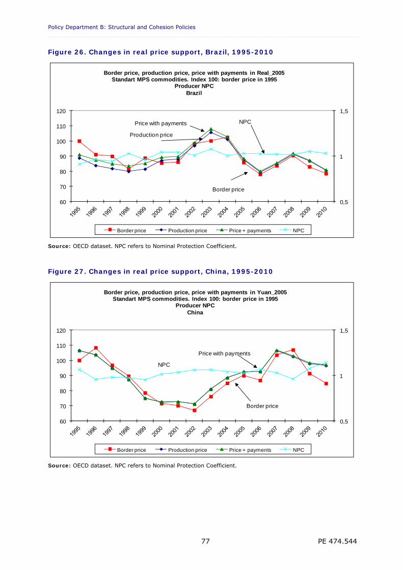
Policy Department B: Structural and Cohesion Policies _________________________________________________________________________________
PE 474.544 77
Figure 26. Changes in real price support, Brazil, 1995-2010
0,5
1
1,5
60
70
80
90
100
110
120
Border price, production price, price with payments in Real_2005Standart MPS commodities. Index 100: border price in 1995
Producer NPCBrazil
Border price Production price Price + payments NPC
Border price
Production price
Price with payments NPC
Source: OECD dataset. NPC refers to Nominal Protection Coefficient.
Figure 27. Changes in real price support, China, 1995-2010
0,5
1
1,5
60
70
80
90
100
110
120
Border price, production price, price with payments in Yuan_2005Standart MPS commodities. Index 100: border price in 1995
Producer NPCChina
Border price Production price Price + payments NPC
Border price
Price with payments
NPC
Source: OECD dataset. NPC refers to Nominal Protection Coefficient.
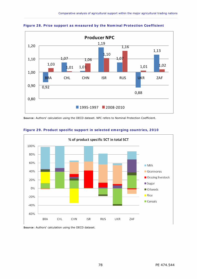
Comparative analysis of agricultural support within the major agricultural trading nations ___________________________________________________________________________________________
PE 474.544 78
Figure 28. Price support as measured by the Nominal Protection Coefficient
0,92
1,07
1,01
1,19
1,07
0,88
1,13
1,031,01
1,06
1,10
1,16
1,01 1,02
0,80
0,90
1,00
1,10
1,20
BRA CHL CHN ISR RUS UKR ZAF
Producer NPC
1995‐1997 2008‐2010
Source: Authors' calculation using the OECD dataset. NPC refers to Nominal Protection Coefficient.
Figure 29. Product specific support in selected emerging countries, 2010
Source: Authors' calculation using the OECD dataset.
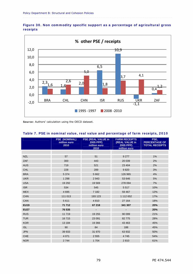
Policy Department B: Structural and Cohesion Policies _________________________________________________________________________________
PE 474.544 79
Figure 30. Non commodity specific support as a percentage of agricultural gross receipts
Source: Authors' calculation using the OECD dataset.
Table 7. PSE in nominal value, real value and percentage of farm receipts, 2010
PSE (NOMINAL) million euro
2010
PSE (REAL VALUE in 2005 PPP)
million euro 2010
FARM RECEIPTS (REAL VALUE in
2005 PPP) million euro
PSE, PERCENTAGE OF TOTAL RECEIPTS
NZL 57 51 9 277 1%
ZAF 300 443 20 039 2%
AUS 719 521 23 404 2%
CHL 228 289 9 820 3%
BRA 5 374 5 662 126 965 4%
UKR 1 298 2 943 53 646 5%
USA 19 292 19 569 278 094 7%
ISR 534 545 5 517 10%
MEX 4 695 7 182 59 467 12%
CHN 111 013 193 123 1 112 652 17%
CAN 5 611 4 810 27 164 18%
EU19 71 712 67 218 341 307 20%
EU27 76 535 - - 20%
RUS 11 719 19 255 90 099 21%
TUR 16 715 23 091 82 775 28%
KOR 13 184 19 366 43 463 45%
ISL 90 84 188 45%
JPN 39 933 31 970 63 932 50%
CHE 4 071 2 555 4 745 54%
NOR 2 744 1 704 2 810 61%
2,31,4
2,0
6,5
10,9
‐ 1,1
0,4 1,6
2,6
5,0
1,8
3,7 4,1
1,2
‐ 2,0
0,0
2,0
4,0
6,0
8,0
10,0
12,0
BRA CHL CHN ISR RUS UKR ZAF
% other PSE / receipts
1995 ‐ 1997 2008 ‐ 2010
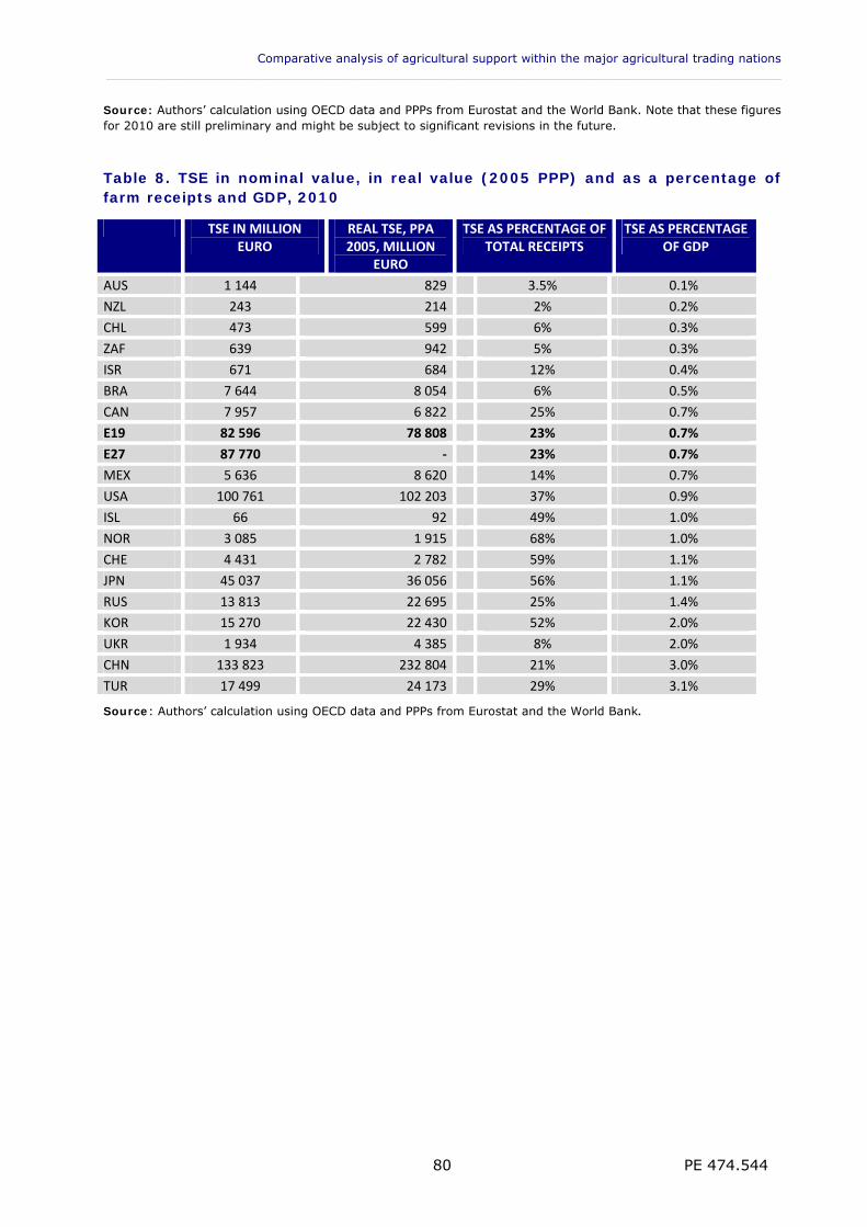
Comparative analysis of agricultural support within the major agricultural trading nations ___________________________________________________________________________________________
PE 474.544 80
Source: Authors’ calculation using OECD data and PPPs from Eurostat and the World Bank. Note that these figures for 2010 are still preliminary and might be subject to significant revisions in the future.
Table 8. TSE in nominal value, in real value (2005 PPP) and as a percentage of farm receipts and GDP, 2010
TSE IN MILLION EURO
REAL TSE, PPA 2005, MILLION
EURO
TSE AS PERCENTAGE OF TOTAL RECEIPTS
TSE AS PERCENTAGE OF GDP
AUS 1 144 829 3.5% 0.1%
NZL 243 214 2% 0.2%
CHL 473 599 6% 0.3%
ZAF 639 942 5% 0.3%
ISR 671 684 12% 0.4%
BRA 7 644 8 054 6% 0.5%
CAN 7 957 6 822 25% 0.7%
E19 82 596 78 808 23% 0.7%
E27 87 770 ‐ 23% 0.7%
MEX 5 636 8 620 14% 0.7%
USA 100 761 102 203 37% 0.9%
ISL 66 92 49% 1.0%
NOR 3 085 1 915 68% 1.0%
CHE 4 431 2 782 59% 1.1%
JPN 45 037 36 056 56% 1.1%
RUS 13 813 22 695 25% 1.4%
KOR 15 270 22 430 52% 2.0%
UKR 1 934 4 385 8% 2.0%
CHN 133 823 232 804 21% 3.0%
TUR 17 499 24 173 29% 3.1%
Source: Authors’ calculation using OECD data and PPPs from Eurostat and the World Bank.
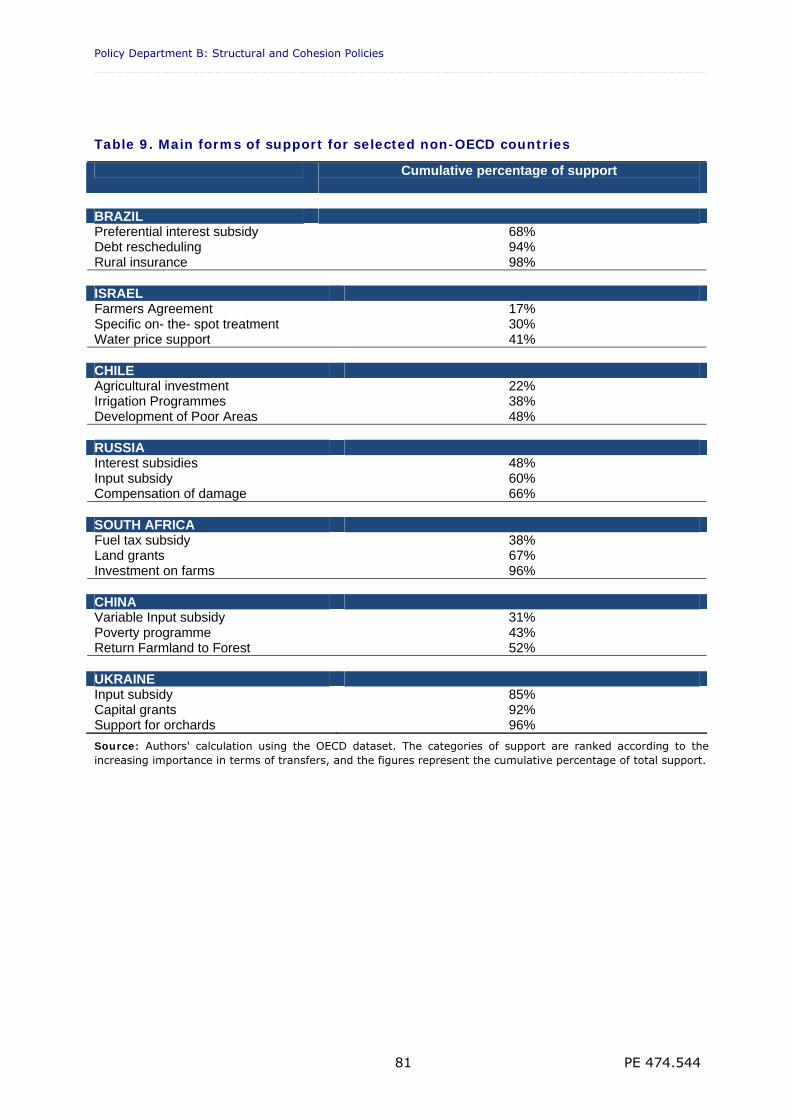
Policy Department B: Structural and Cohesion Policies _________________________________________________________________________________
PE 474.544 81
Table 9. Main forms of support for selected non-OECD countries
Cumulative percentage of support
BRAZIL Preferential interest subsidy 68% Debt rescheduling 94% Rural insurance 98% ISRAEL Farmers Agreement 17% Specific on- the- spot treatment 30% Water price support 41% CHILE Agricultural investment 22% Irrigation Programmes 38% Development of Poor Areas 48% RUSSIA Interest subsidies 48% Input subsidy 60% Compensation of damage 66% SOUTH AFRICA Fuel tax subsidy 38% Land grants 67% Investment on farms 96% CHINA Variable Input subsidy 31% Poverty programme 43% Return Farmland to Forest 52% UKRAINE Input subsidy 85% Capital grants 92% Support for orchards 96%
Source: Authors' calculation using the OECD dataset. The categories of support are ranked according to the increasing importance in terms of transfers, and the figures represent the cumulative percentage of total support.
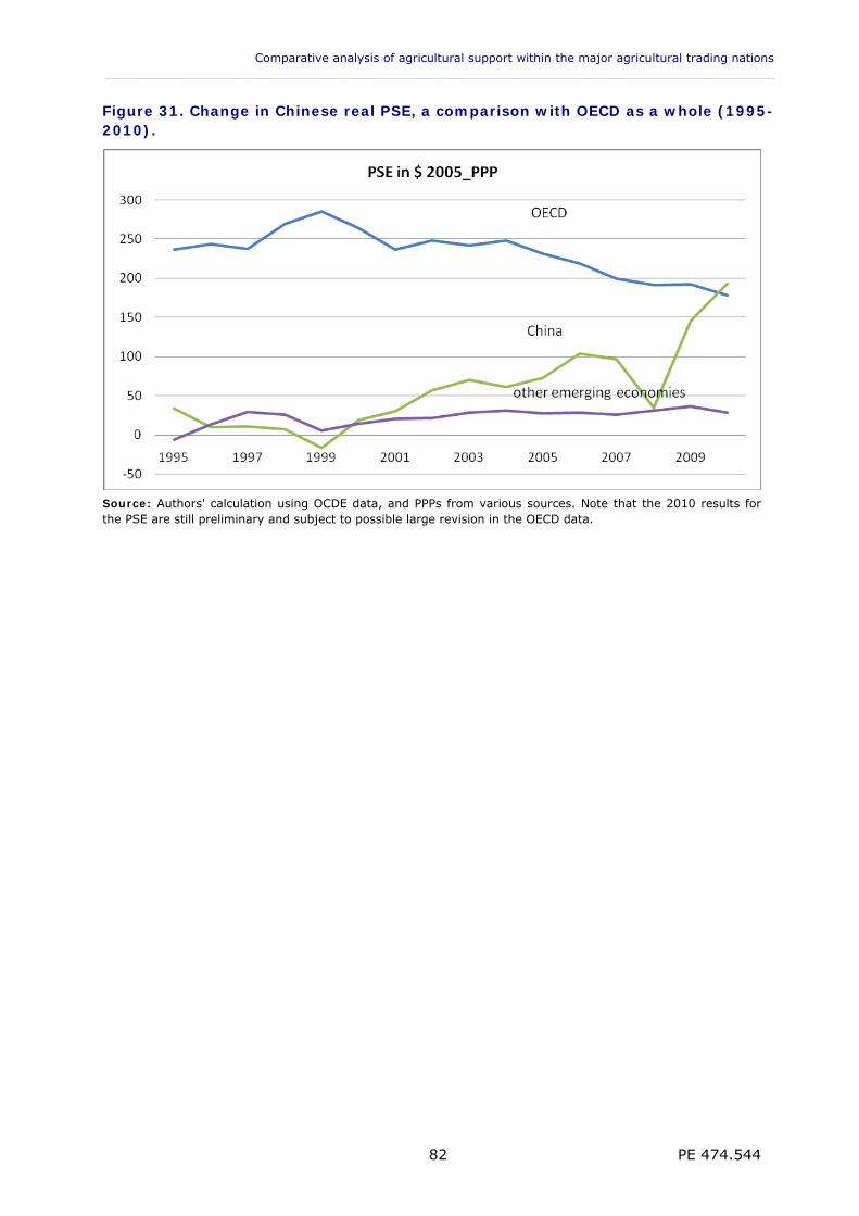
Comparative analysis of agricultural support within the major agricultural trading nations ___________________________________________________________________________________________
PE 474.544 82
Figure 31. Change in Chinese real PSE, a comparison with OECD as a whole (1995-2010).
Source: Authors' calculation using OCDE data, and PPPs from various sources. Note that the 2010 results for the PSE are still preliminary and subject to possible large revision in the OECD data.
Policy Department B: Structural and Cohesion Policies _________________________________________________________________________________
PE 474.544 83
4. AGRICULTURAL SUPPORT IN THE EU
KEY FINDINGS Support to EU agriculture is assessed using a variety of sources, i.e., economic
accounts, farm level survey data, and OECD as well as WTO notifications.
Neither macro nor microeconomic data accounts for the support that is provided through prices, but rather they provide useful information regarding subsidies actually received by farmers (both national and EU funded). In the EU, subsidies per family worker went up from €7500 to €12000 (constant 2005 euro) between 1995 and 2008. Subsidies went from 47% of the family income in 1995 to 60% in 2008.
EU support has moved towards more decoupled direct payments, is less and less product specific and therefore more and more production neutral. It now has a limited impact on world markets.
While direct payments are now the largest part of EU support, there are still some very large transfers to farmers through fuel subsidies (tax rebates). The latter are as large as agri-environmental payments.
International (WTO) commitments on domestic support constrain the AMS, an indicator that has little economic relevance. However, the EU AMS is now less than 20% of the authorized ceiling.
Neither the OECD nor the WTO takes biofuel policies into account in the measures that support farmers, even though they now play an important role in the EU and the US.
4.1. Changes in the structure of agricultural support in the EU
The CAP of the 1960s to 1980s relied heavily on measures that supported prices. At the end of the 1980s, the domestic price of cereals was more than 2.5 times higher the world price, suggesting that considerable transfers took place from consumers (in particular from the animal feed sector, hence livestock farmers) to grain producers. The high level of protection and the supply control granted to sugar and dairy production also led to considerable transfers from consumers to producers. At the same time, taxpayers were asked to contribute significantly to a growing CAP budget, given the need to get rid of surplus production, resulting in storage costs and export refunds. 24 Since 1992, successive reforms of the CAP have followed a consistent path. Institutional prices were reduced progressively and the system of intervention (i.e., government purchases when prices go below a certain threshold) was made explicitly or de facto inactive for several major commodities including beef, sugar and coarse grains. In the cereal, oilseed, protein seed and beef sectors, the corresponding losses in income were compensated by direct payments. Until 2008, they were subject to production limiting conditions (obligation of setting land aside; a cap per number of heads per hectare; a cap on national payments) and were based on fixed yields. The shift towards single farm payments between 2003 and 2008 completed the move towards a form of support that is largely production neutral. These reforms have made it possible to solve major disequilibria, including the costly market imbalance for cereals.
24 See EP (2007; 2010); Bureau (2008); Ritson and Harvey (1997) for an introduction to these issues.
Comparative analysis of agricultural support within the major agricultural trading nations ___________________________________________________________________________________________
PE 474.544 84
In parallel, it was increasingly recognised that certain types of agriculture delivered environmental benefits and that farmers providing these benefits needed to be remunerated via public support. The Agenda 2000 reforms served to deepen the reform process, with greater support for rural development. It resulted in the emergence of a "second pillar" of the CAP. An administrative and financial framework - with common objectives and a single set of programming, financing, monitoring and auditing rules - was progressively implemented for EU rural development policy. Today’s CAP Pillar 1 includes market measures as well as more decoupled direct payments supporting income (including the Single Farm Payment scheme or SFP and the Single Area Payment Scheme or SAPS, available to new Member States) and a few coupled payments that have persisted. Pillar 1 is funded under the European Agricultural Guarantee Fund (EAGF), the main expenditures being direct payments to farmers and measures to regulate agricultural markets such as intervention purchasing, and the remaining export refunds. The CAP Pillar 2 - "Rural Development" - is a common policy with strategic objectives set at the EU level. It is directed at enhancing the environment and countryside, improving competitiveness of EU agriculture and forestry and improving the quality of life in rural areas and is funded under the European Agricultural Fund for Rural Development (EAFRD) for the programming period 2007 – 2013. While the budget devoted to agricultural policy has remained large, reforms have reduced some expenditure such as storage costs and export subsidies. Payments now benefit farmers more directly, and their more decoupled nature has reduced the negative effects of the CAP on world prices and third country producers. Reforms have also increased the legitimacy of the policy, with a change in objectives making the policy more in line with societal demands. The various indicators proposed to measure the level of farm support in the EU, and to assess the changes in the composition of support acknowledge that some considerable progress has been made over the last two decades. In particular both the OECD product specific PSEs and the WTO AMS have gone down considerably while measures of total support remained more stable. This reflects not only a reduction in the market price support but also a shift of support towards rural development (Figure 32 and Figure 33). The OECD monitoring of agricultural policies also shows clearly that, in the EU, a shift has taken place towards policies that were less distorting and more efficient at transferring income to farmers (OECD 2011).
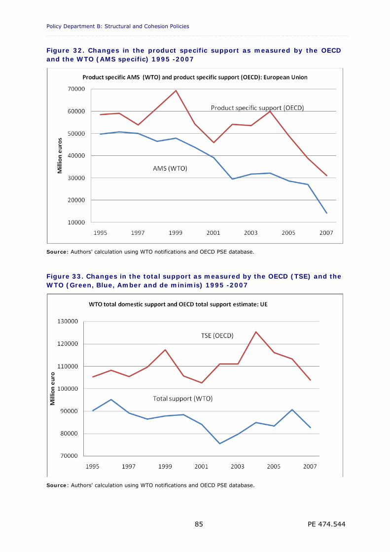
Policy Department B: Structural and Cohesion Policies _________________________________________________________________________________
PE 474.544 85
Figure 32. Changes in the product specific support as measured by the OECD and the WTO (AMS specific) 1995 -2007
Source: Authors' calculation using WTO notifications and OECD PSE database.
Figure 33. Changes in the total support as measured by the OECD (TSE) and the WTO (Green, Blue, Amber and de minimis) 1995 -2007
Source: Authors' calculation using WTO notifications and OECD PSE database.
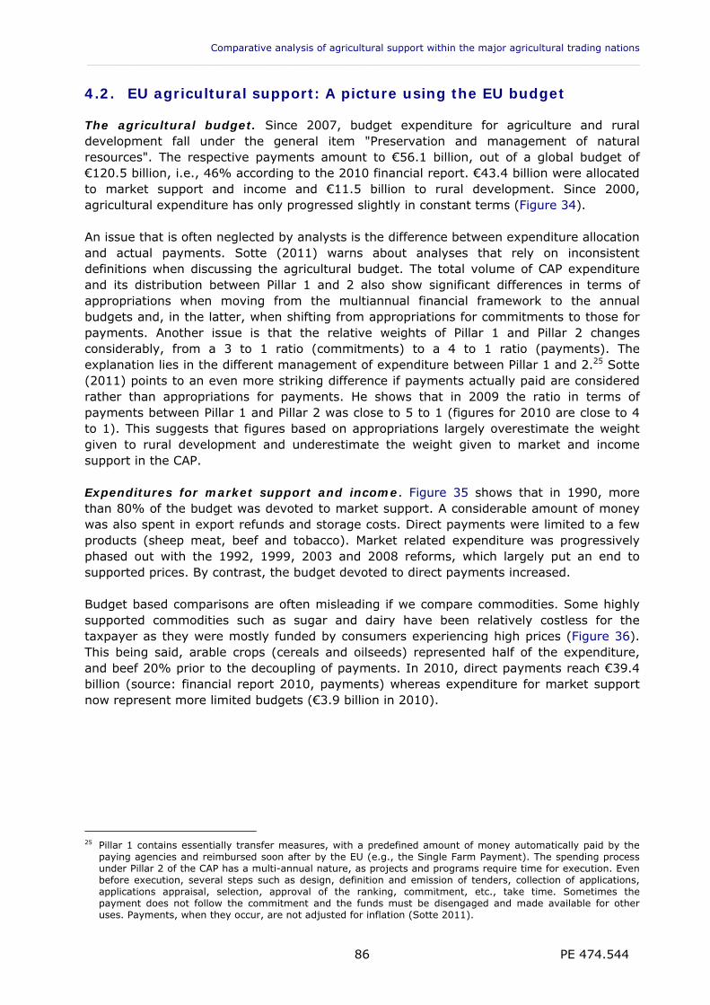
Comparative analysis of agricultural support within the major agricultural trading nations ___________________________________________________________________________________________
PE 474.544 86
4.2. EU agricultural support: A picture using the EU budget
The agricultural budget. Since 2007, budget expenditure for agriculture and rural development fall under the general item "Preservation and management of natural resources". The respective payments amount to €56.1 billion, out of a global budget of €120.5 billion, i.e., 46% according to the 2010 financial report. €43.4 billion were allocated to market support and income and €11.5 billion to rural development. Since 2000, agricultural expenditure has only progressed slightly in constant terms (Figure 34). An issue that is often neglected by analysts is the difference between expenditure allocation and actual payments. Sotte (2011) warns about analyses that rely on inconsistent definitions when discussing the agricultural budget. The total volume of CAP expenditure and its distribution between Pillar 1 and 2 also show significant differences in terms of appropriations when moving from the multiannual financial framework to the annual budgets and, in the latter, when shifting from appropriations for commitments to those for payments. Another issue is that the relative weights of Pillar 1 and Pillar 2 changes considerably, from a 3 to 1 ratio (commitments) to a 4 to 1 ratio (payments). The explanation lies in the different management of expenditure between Pillar 1 and 2.25 Sotte (2011) points to an even more striking difference if payments actually paid are considered rather than appropriations for payments. He shows that in 2009 the ratio in terms of payments between Pillar 1 and Pillar 2 was close to 5 to 1 (figures for 2010 are close to 4 to 1). This suggests that figures based on appropriations largely overestimate the weight given to rural development and underestimate the weight given to market and income support in the CAP. Expenditures for market support and income. Figure 35 shows that in 1990, more than 80% of the budget was devoted to market support. A considerable amount of money was also spent in export refunds and storage costs. Direct payments were limited to a few products (sheep meat, beef and tobacco). Market related expenditure was progressively phased out with the 1992, 1999, 2003 and 2008 reforms, which largely put an end to supported prices. By contrast, the budget devoted to direct payments increased. Budget based comparisons are often misleading if we compare commodities. Some highly supported commodities such as sugar and dairy have been relatively costless for the taxpayer as they were mostly funded by consumers experiencing high prices (Figure 36). This being said, arable crops (cereals and oilseeds) represented half of the expenditure, and beef 20% prior to the decoupling of payments. In 2010, direct payments reach €39.4 billion (source: financial report 2010, payments) whereas expenditure for market support now represent more limited budgets (€3.9 billion in 2010).
25 Pillar 1 contains essentially transfer measures, with a predefined amount of money automatically paid by the
paying agencies and reimbursed soon after by the EU (e.g., the Single Farm Payment). The spending process under Pillar 2 of the CAP has a multi-annual nature, as projects and programs require time for execution. Even before execution, several steps such as design, definition and emission of tenders, collection of applications, applications appraisal, selection, approval of the ranking, commitment, etc., take time. Sometimes the payment does not follow the commitment and the funds must be disengaged and made available for other uses. Payments, when they occur, are not adjusted for inflation (Sotte 2011).
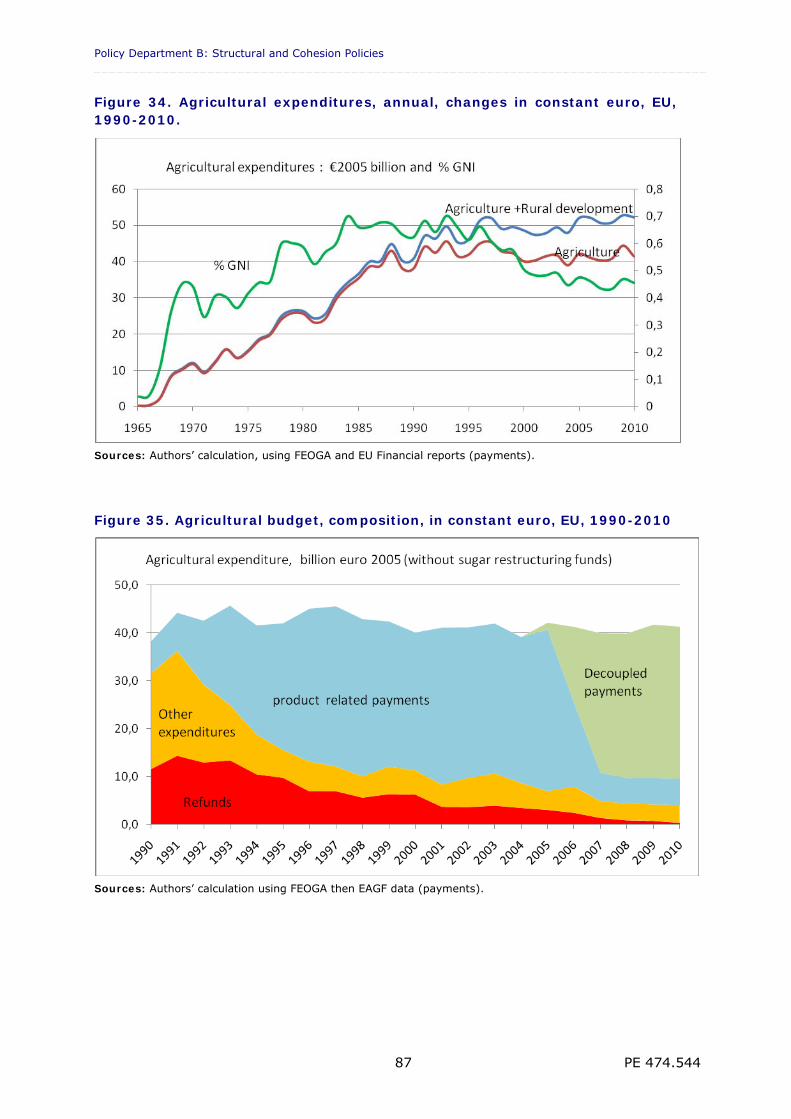
Policy Department B: Structural and Cohesion Policies _________________________________________________________________________________
PE 474.544 87
Figure 34. Agricultural expenditures, annual, changes in constant euro, EU, 1990-2010.
Sources: Authors’ calculation, using FEOGA and EU Financial reports (payments).
Figure 35. Agricultural budget, composition, in constant euro, EU, 1990-2010
Sources: Authors’ calculation using FEOGA then EAGF data (payments).
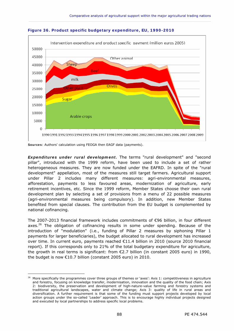
Comparative analysis of agricultural support within the major agricultural trading nations ___________________________________________________________________________________________
PE 474.544 88
Figure 36. Product specific budgetary expenditure, EU, 1990-2010
Sources: Authors' calculation using FEOGA then EAGF data (payments).
Expenditures under rural development. The terms "rural development" and "second pillar", introduced with the 1999 reform, have been used to include a set of rather heterogeneous measures. They are now funded under the EAFRD. In spite of the "rural development" appellation, most of the measures still target farmers. Agricultural support under Pillar 2 includes many different measures: agri-environmental measures, afforestation, payments to less favoured areas, modernization of agriculture, early retirement incentives, etc. Since the 1999 reform, Member States choose their own rural development plan by selecting a set of provisions from a menu of 22 possible measures (agri-environmental measures being compulsory). In addition, new Member States benefited from special clauses. The contribution from the EU budget is complemented by national cofinancing. The 2007-2013 financial framework includes commitments of €96 billion, in four different axes.26 The obligation of cofinancing results in some under spending. Because of the introduction of "modulation" (i.e., funding of Pillar 2 measures by siphoning Pillar 1 payments for larger beneficiaries), the budget allocated to rural development has increased over time. In current euro, payments reached €11.4 billion in 2010 (source 2010 financial report). If this corresponds only to 21% of the total budgetary expenditure for agriculture, the growth in real terms is significant: from €2.7 billion (in constant 2005 euro) in 1990, the budget is now €10.7 billion (constant 2005 euro) in 2010.
26 More specifically the programmes cover three groups of themes or ‘axes’: Axis 1: competitiveness in agriculture
and forestry, focusing on knowledge transfer, modernisation, innovation and the quality of the food chain; Axis 2: biodiversity, the preservation and development of high-nature-value farming and forestry systems and traditional agricultural landscapes, water and climate change; Axis 3: quality of life in rural areas and diversification. A further requirement is that some of the funding must support projects developed by local action groups under the so-called ‘Leader’ approach. This is to encourage highly individual projects designed and executed by local partnerships to address specific local problems.
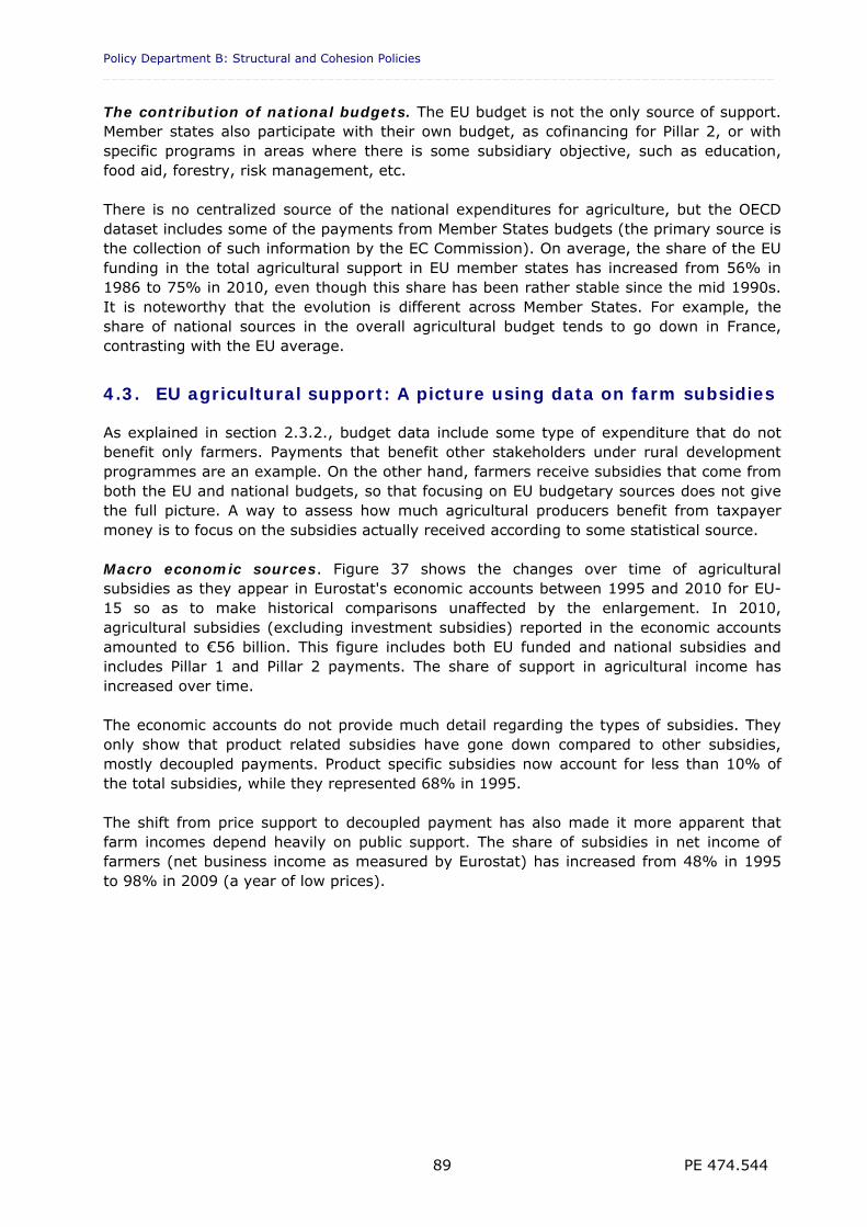
Policy Department B: Structural and Cohesion Policies _________________________________________________________________________________
PE 474.544 89
The contribution of national budgets. The EU budget is not the only source of support. Member states also participate with their own budget, as cofinancing for Pillar 2, or with specific programs in areas where there is some subsidiary objective, such as education, food aid, forestry, risk management, etc. There is no centralized source of the national expenditures for agriculture, but the OECD dataset includes some of the payments from Member States budgets (the primary source is the collection of such information by the EC Commission). On average, the share of the EU funding in the total agricultural support in EU member states has increased from 56% in 1986 to 75% in 2010, even though this share has been rather stable since the mid 1990s. It is noteworthy that the evolution is different across Member States. For example, the share of national sources in the overall agricultural budget tends to go down in France, contrasting with the EU average.
4.3. EU agricultural support: A picture using data on farm subsidies
As explained in section 2.3.2., budget data include some type of expenditure that do not benefit only farmers. Payments that benefit other stakeholders under rural development programmes are an example. On the other hand, farmers receive subsidies that come from both the EU and national budgets, so that focusing on EU budgetary sources does not give the full picture. A way to assess how much agricultural producers benefit from taxpayer money is to focus on the subsidies actually received according to some statistical source. Macro economic sources. Figure 37 shows the changes over time of agricultural subsidies as they appear in Eurostat's economic accounts between 1995 and 2010 for EU-15 so as to make historical comparisons unaffected by the enlargement. In 2010, agricultural subsidies (excluding investment subsidies) reported in the economic accounts amounted to €56 billion. This figure includes both EU funded and national subsidies and includes Pillar 1 and Pillar 2 payments. The share of support in agricultural income has increased over time. The economic accounts do not provide much detail regarding the types of subsidies. They only show that product related subsidies have gone down compared to other subsidies, mostly decoupled payments. Product specific subsidies now account for less than 10% of the total subsidies, while they represented 68% in 1995. The shift from price support to decoupled payment has also made it more apparent that farm incomes depend heavily on public support. The share of subsidies in net income of farmers (net business income as measured by Eurostat) has increased from 48% in 1995 to 98% in 2009 (a year of low prices).
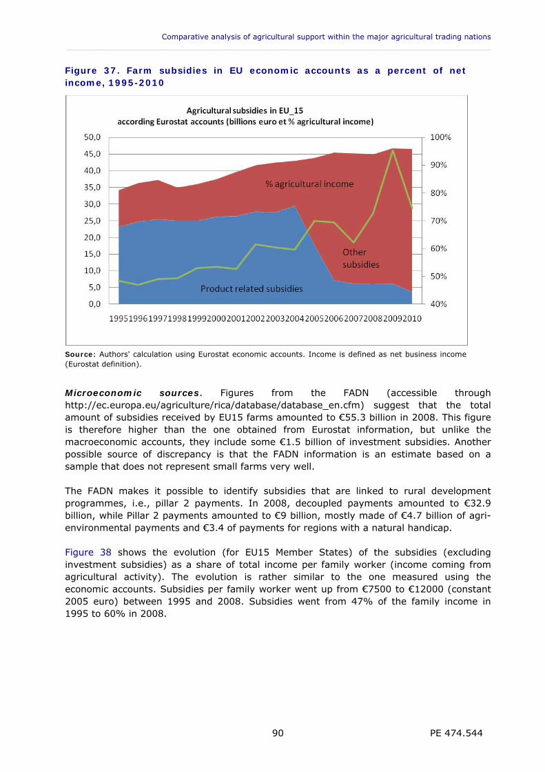
Comparative analysis of agricultural support within the major agricultural trading nations ___________________________________________________________________________________________
PE 474.544 90
Figure 37. Farm subsidies in EU economic accounts as a percent of net income, 1995-2010
Source: Authors' calculation using Eurostat economic accounts. Income is defined as net business income (Eurostat definition).
Microeconomic sources. Figures from the FADN (accessible through http://ec.europa.eu/agriculture/rica/database/database_en.cfm) suggest that the total amount of subsidies received by EU15 farms amounted to €55.3 billion in 2008. This figure is therefore higher than the one obtained from Eurostat information, but unlike the macroeconomic accounts, they include some €1.5 billion of investment subsidies. Another possible source of discrepancy is that the FADN information is an estimate based on a sample that does not represent small farms very well. The FADN makes it possible to identify subsidies that are linked to rural development programmes, i.e., pillar 2 payments. In 2008, decoupled payments amounted to €32.9 billion, while Pillar 2 payments amounted to €9 billion, mostly made of €4.7 billion of agri-environmental payments and €3.4 of payments for regions with a natural handicap. Figure 38 shows the evolution (for EU15 Member States) of the subsidies (excluding investment subsidies) as a share of total income per family worker (income coming from agricultural activity). The evolution is rather similar to the one measured using the economic accounts. Subsidies per family worker went up from €7500 to €12000 (constant 2005 euro) between 1995 and 2008. Subsidies went from 47% of the family income in 1995 to 60% in 2008.
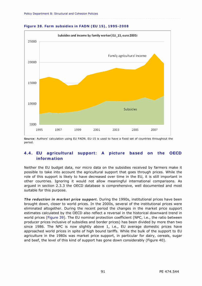
Policy Department B: Structural and Cohesion Policies _________________________________________________________________________________
PE 474.544 91
Figure 38. Farm subsidies in FADN (EU 15), 1995-2008
Source: Authors' calculation using EU FADN. EU-15 is used to have a fixed set of countries throughout the period.
4.4. EU agricultural support: A picture based on the OECD information
Neither the EU budget data, nor micro data on the subsidies received by farmers make it possible to take into account the agricultural support that goes through prices. While the role of this support is likely to have decreased over time in the EU, it is still important in other countries. Ignoring it would not allow meaningful international comparisons. As argued in section 2.3.3 the OECD database is comprehensive, well documented and most suitable for this purpose. The reduction in market price support. During the 1990s, institutional prices have been brought down, closer to world prices. In the 2000s, several of the institutional prices were eliminated altogether. During the recent period the changes in the market price support estimates calculated by the OECD also reflect a reversal in the historical downward trend in world prices (Figure 39). The EU nominal protection coefficient (NPC, i.e., the ratio between producer prices inclusive of subsidies and border prices) has been divided by more than two since 1986. The NPC is now slightly above 1, i.e., EU average domestic prices have approached world prices in spite of high bound tariffs. While the bulk of the support to EU agriculture in the 1980s was market price support, in particular for dairy, cereals, sugar and beef, the level of this kind of support has gone down considerably (Figure 40).
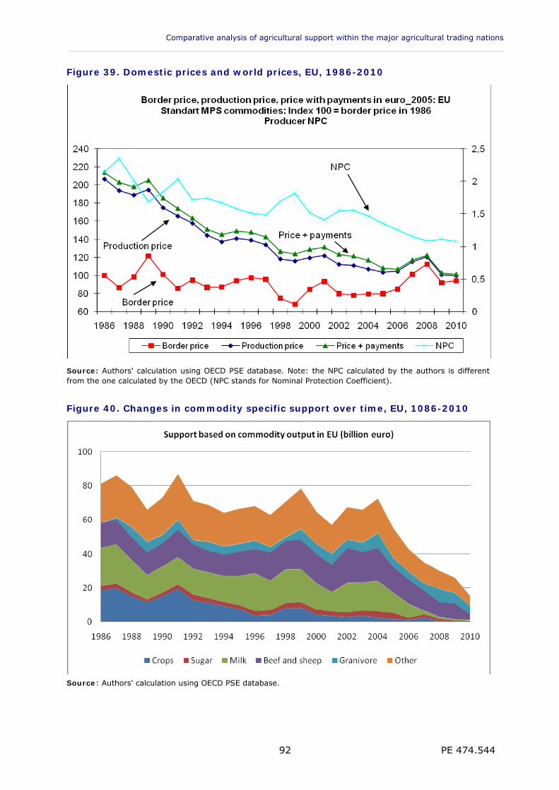
Comparative analysis of agricultural support within the major agricultural trading nations ___________________________________________________________________________________________
PE 474.544 92
Figure 39. Domestic prices and world prices, EU, 1986-2010
Source: Authors' calculation using OECD PSE database. Note: the NPC calculated by the authors is different from the one calculated by the OECD (NPC stands for Nominal Protection Coefficient).
Figure 40. Changes in commodity specific support over time, EU, 1086-2010
Source: Authors' calculation using OECD PSE database.
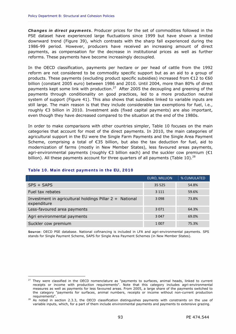
Policy Department B: Structural and Cohesion Policies _________________________________________________________________________________
PE 474.544 93
Changes in direct payments. Producer prices for the set of commodities followed in the PSE dataset have experienced large fluctuations since 1999 but have shown a limited downward trend (Figure 39), which contrasts with the sharp fall experienced during the 1986-99 period. However, producers have received an increasing amount of direct payments, as compensation for the decrease in institutional prices as well as further reforms. These payments have become increasingly decoupled. In the OECD classification, payments per hectare or per head of cattle from the 1992 reform are not considered to be commodity specific support but as an aid to a group of products. These payments (excluding product specific subsidies) increased from €12 to €60 billion (constant 2005 euro) between 1986 and 2010. Until 2004, more than 80% of direct payments kept some link with production.27 After 2005 the decoupling and greening of the payments through conditionality on good practices, led to a more production neutral system of support (Figure 41). This also shows that subsidies linked to variable inputs are still large. The main reason is that they include considerable tax exemptions for fuel, i.e., roughly €3 billion in 2010. Investment aids (fixed capital payments) are also important, even though they have decreased compared to the situation at the end of the 1980s. In order to make comparisons with other countries simpler, Table 10 focuses on the main categories that account for most of the direct payments. In 2010, the main categories of agricultural support in the EU were the Single Farm Payments and the Single Area Payment Scheme, comprising a total of €35 billion, but also the tax deduction for fuel, aid to modernization of farms (mostly in New Member States), less favoured areas payments, agri-environmental payments (roughly €3 billion each) and the suckler cow premium (€1 billion). All these payments account for three quarters of all payments (Table 10).28
Table 10. Main direct payments in the EU, 2010
EURO, MILLION % CUMULATED
SPS + SAPS 35 525 54.8%
Fuel tax rebates 3 111 59.6%
Investment in agricultural holdings Pillar 2 + National expenditure
3 098 73.8%
Less-favoured area payments 3 071 64.3%
Agri environmental payments 3 047 69.0%
Suckler cow premium 1 007 75.3%
Source: OECD PSE database. National cofinancing is included in LFA and agri-environmental payments. SPS stands for Single Payment Scheme, SAPS for Single Area Payment Schemes (in New Member States).
27 They were classified in the OECD nomenclature as "payments to surfaces, animal heads, linked to current
receipts or income with production requirements". Note that this category includes agri-environmental measures as well as payments for less favoured areas. From 2005, a large share of the payments switched to the category "payments for surfaces, animal numbers, receipts or income without non-current production requirements".
28 As noted in section 2.3.3, the OECD classification distinguishes payments with constraints on the use of variable inputs, which, for a part of them include environmental payments and payments to extensive grazing.
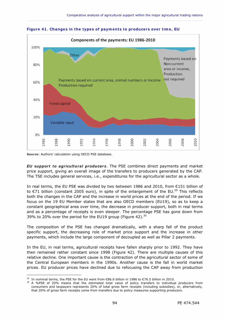
Comparative analysis of agricultural support within the major agricultural trading nations ___________________________________________________________________________________________
PE 474.544 94
Figure 41. Changes in the types of payments to producers over time, EU
Source: Authors' calculation using OECD PSE database.
EU support to agricultural producers. The PSE combines direct payments and market price support, giving an overall image of the transfers to producers generated by the CAP. The TSE includes general services, i.e., expenditures for the agricultural sector as a whole. In real terms, the EU PSE was divided by two between 1986 and 2010, from €151 billion of to €71 billion (constant 2005 euro), in spite of the enlargement of the EU.29 This reflects both the changes in the CAP and the increase in world prices at the end of the period. If we focus on the 19 EU Member states that are also OECD members (EU19), so as to keep a constant geographical area over time, the decrease in producer support, both in real terms and as a percentage of receipts is even steeper. The percentage PSE has gone down from 39% to 20% over the period for the EU19 group (Figure 42).30 The composition of the PSE has changed dramatically, with a sharp fall of the product specific support, the decreasing role of market price support and the increase in other payments, which include the large component of decoupled as well as Pillar 2 payments. In the EU, in real terms, agricultural receipts have fallen sharply prior to 1992. They have then remained rather constant since 1998 (Figure 42). There are multiple causes of this relative decline. One important cause is the contraction of the agricultural sector of some of the Central European members in the 1990s. Another cause is the fall in world market prices. EU producer prices have declined due to refocusing the CAP away from production
29 In nominal terms, the PSE for the EU went from €86.6 billion in 1986 to €76.5 billion in 2010. 30 A %PSE of 20% means that the estimated total value of policy transfers to individual producers from
consumers and taxpayers represents 20% of total gross farm receipts (including subsidies), or, alternatively, that 20% of gross farm receipts come from transfers due to policy measures supporting producers.
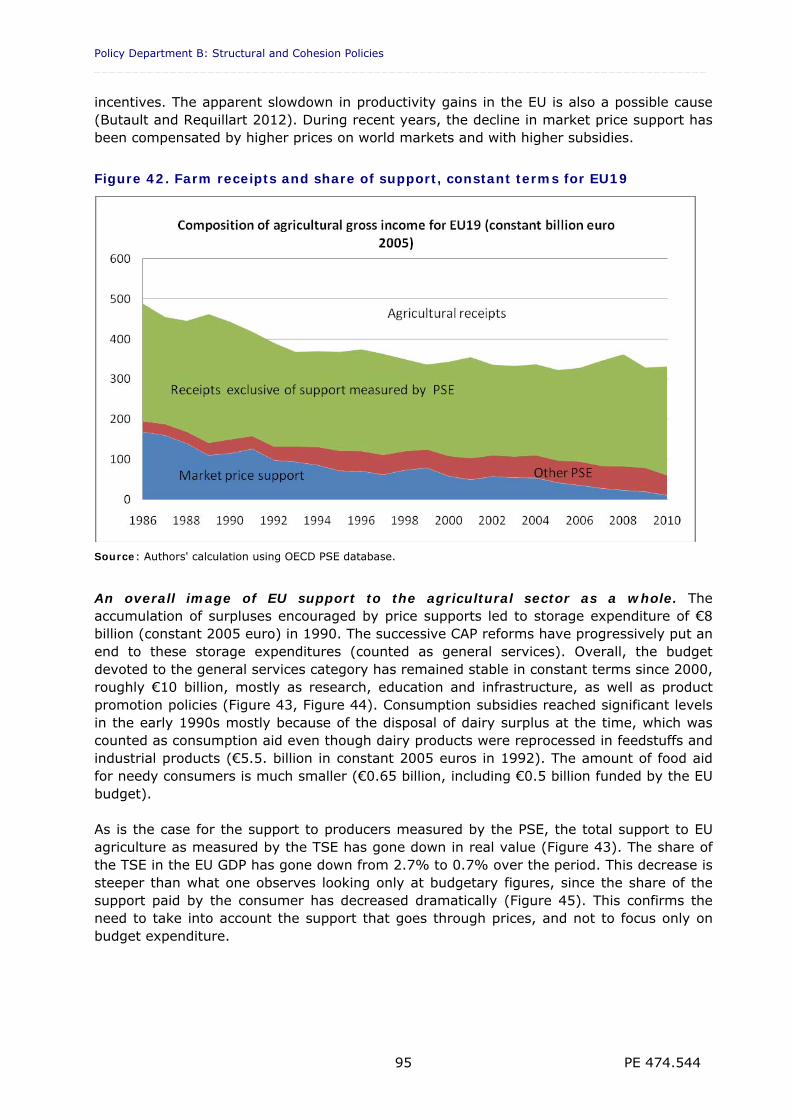
Policy Department B: Structural and Cohesion Policies _________________________________________________________________________________
PE 474.544 95
incentives. The apparent slowdown in productivity gains in the EU is also a possible cause (Butault and Requillart 2012). During recent years, the decline in market price support has been compensated by higher prices on world markets and with higher subsidies.
Figure 42. Farm receipts and share of support, constant terms for EU19
Source: Authors' calculation using OECD PSE database.
An overall image of EU support to the agricultural sector as a whole. The accumulation of surpluses encouraged by price supports led to storage expenditure of €8 billion (constant 2005 euro) in 1990. The successive CAP reforms have progressively put an end to these storage expenditures (counted as general services). Overall, the budget devoted to the general services category has remained stable in constant terms since 2000, roughly €10 billion, mostly as research, education and infrastructure, as well as product promotion policies (Figure 43, Figure 44). Consumption subsidies reached significant levels in the early 1990s mostly because of the disposal of dairy surplus at the time, which was counted as consumption aid even though dairy products were reprocessed in feedstuffs and industrial products (€5.5. billion in constant 2005 euros in 1992). The amount of food aid for needy consumers is much smaller (€0.65 billion, including €0.5 billion funded by the EU budget). As is the case for the support to producers measured by the PSE, the total support to EU agriculture as measured by the TSE has gone down in real value (Figure 43). The share of the TSE in the EU GDP has gone down from 2.7% to 0.7% over the period. This decrease is steeper than what one observes looking only at budgetary figures, since the share of the support paid by the consumer has decreased dramatically (Figure 45). This confirms the need to take into account the support that goes through prices, and not to focus only on budget expenditure.
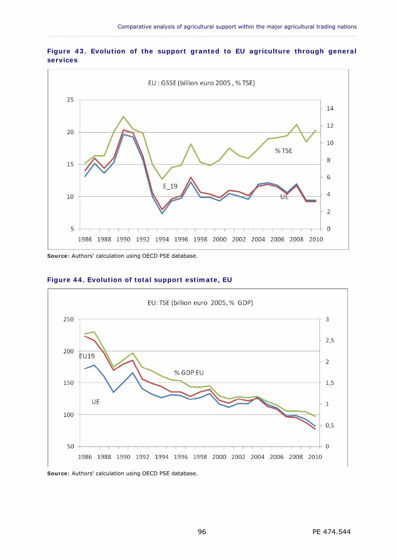
Comparative analysis of agricultural support within the major agricultural trading nations ___________________________________________________________________________________________
PE 474.544 96
Figure 43. Evolution of the support granted to EU agriculture through general services
Source: Authors' calculation using OECD PSE database.
Figure 44. Evolution of total support estimate, EU
Source: Authors' calculation using OECD PSE database.
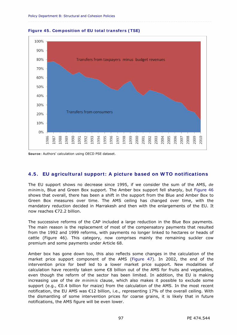
Policy Department B: Structural and Cohesion Policies _________________________________________________________________________________
PE 474.544 97
Figure 45. Composition of EU total transfers (TSE)
Source: Authors' calculation using OECD PSE dataset.
4.5. EU agricultural support: A picture based on WTO notifications
The EU support shows no decrease since 1995, if we consider the sum of the AMS, de minimis, Blue and Green Box support. The Amber box support fell sharply, but Figure 46 shows that overall, there has been a shift in the support from the Blue and Amber Box to Green Box measures over time. The AMS ceiling has changed over time, with the mandatory reduction decided in Marrakesh and then with the enlargements of the EU. It now reaches €72.2 billion. The successive reforms of the CAP included a large reduction in the Blue Box payments. The main reason is the replacement of most of the compensatory payments that resulted from the 1992 and 1999 reforms, with payments no longer linked to hectares or heads of cattle (Figure 46). This category, now comprises mainly the remaining suckler cow premium and some payments under Article 68. Amber box has gone down too, this also reflects some changes in the calculation of the market price support component of the AMS (Figure 47). In 2002, the end of the intervention price for beef led to a lower market price support. New modalities of calculation have recently taken some €8 billion out of the AMS for fruits and vegetables, even though the reform of the sector has been limited. In addition, the EU is making increasing use of the de minimis clause, which also makes it possible to exclude some support (e.g., €0.4 billion for maize) from the calculation of the AMS. In the most recent notification, the EU AMS was €12 billion, i.e., representing 17% of the overall ceiling. With the dismantling of some intervention prices for coarse grains, it is likely that in future notifications, the AMS figure will be even lower.
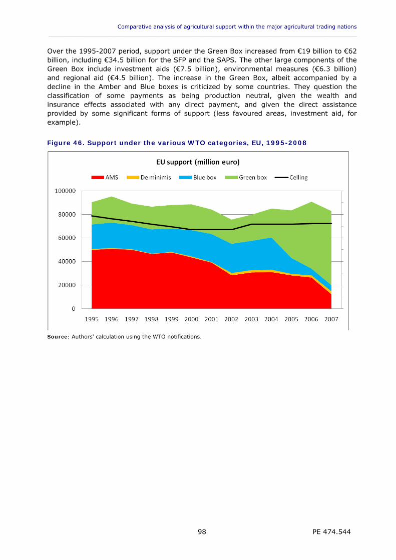
Comparative analysis of agricultural support within the major agricultural trading nations ___________________________________________________________________________________________
PE 474.544 98
Over the 1995-2007 period, support under the Green Box increased from €19 billion to €62 billion, including €34.5 billion for the SFP and the SAPS. The other large components of the Green Box include investment aids (€7.5 billion), environmental measures (€6.3 billion) and regional aid (€4.5 billion). The increase in the Green Box, albeit accompanied by a decline in the Amber and Blue boxes is criticized by some countries. They question the classification of some payments as being production neutral, given the wealth and insurance effects associated with any direct payment, and given the direct assistance provided by some significant forms of support (less favoured areas, investment aid, for example).
Figure 46. Support under the various WTO categories, EU, 1995-2008
Source: Authors' calculation using the WTO notifications.
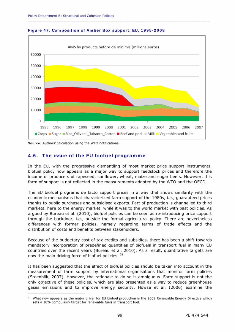
Policy Department B: Structural and Cohesion Policies _________________________________________________________________________________
PE 474.544 99
Figure 47. Composition of Amber Box support, EU, 1995-2008
Source: Authors' calculation using the WTO notifications.
4.6. The issue of the EU biofuel programme
In the EU, with the progressive dismantling of most market price support instruments, biofuel policy now appears as a major way to support feedstock prices and therefore the income of producers of rapeseed, sunflower, wheat, maize and sugar beets. However, this form of support is not reflected in the measurements adopted by the WTO and the OECD. The EU biofuel programs de facto support prices in a way that shows similarity with the economic mechanisms that characterized farm support of the 1980s, i.e., guaranteed prices thanks to public purchases and subsidised exports. Part of production is channelled to third markets, here to the energy market, while it was to the world market with past policies. As argued by Bureau et al. (2010), biofuel policies can be seen as re-introducing price support through the backdoor, i.e., outside the formal agricultural policy. There are nevertheless differences with former policies, namely regarding terms of trade effects and the distribution of costs and benefits between stakeholders. Because of the budgetary cost of tax credits and subsidies, there has been a shift towards mandatory incorporation of predefined quantities of biofuels in transport fuel in many EU countries over the recent years (Bureau et al. 2010). As a result, quantitative targets are now the main driving force of biofuel policies. 31 It has been suggested that the effect of biofuel policies should be taken into account in the measurement of farm support by international organisations that monitor farm policies (Steenblik, 2007). However, the rationale to do so is ambiguous. Farm support is not the only objective of these policies, which are also presented as a way to reduce greenhouse gases emissions and to improve energy security. Howse et al. (2006) examine the 31 What now appears as the major driver for EU biofuel production is the 2009 Renewable Energy Directive which
sets a 10% compulsory target for renewable fuels in transport fuel.
Comparative analysis of agricultural support within the major agricultural trading nations ___________________________________________________________________________________________
PE 474.544 100
compatibility of biofuel tax credits and tariffs and WTO agreements and question their qualification as distorting subsidies. Josling et al. (2010) also raise technical issues which oppose making biofuel support subject to WTO discipline. The incidence of biofuel subsidies, which are provided at different levels of the supply chain, is difficult to assess due to complex pass-through between blenders, processors and farmers. Their opinion is also that the incorporation of the subsidy effect of biofuel mandates into the PSEs is questionable. The objective of the PSE is to measure the impact on producers of the actions of their own government, and it would be difficult to endogenize the (world) reference price, for both conceptual and political reasons. Still, there is no doubt that biofuel policies support farmers. Bureau et al. (2010) attempt to assess the level of support to EU and US agriculture that is implicitly provided by the biofuel mandates. They consider the case of support to rapeseed producers through the bioenergy mandate. Considering the structure of the current EU industry and substitution effects, the biodiesel component of the EU incorporation mandate, is equivalent to a 22% increase in the EU rapeseed production price compared to the reference situation. They then compare this benchmark scenario to a counterfactual scenario in which the EU supports rapeseed producers with a system of coupled direct payments, like the one that characterized the EU oilseeds policy in the 1980s. In order to obtain a similar price for EU rapeseed producers, at an oil price of USD 60 a barrel, the corresponding payment would have to reach €1.5 billion. Supporting agricultural producers through such an outlet does not put the burden of the support on the same stakeholders. Should rapeseed producers be supported by a system of direct payments instead of the biofuel mandate, the EU price of diesel blend would be 2.7% lower for consumers (on an energy equivalent basis). The price of rapeseed paid by the food industry would also be much lower (-22.7%). That is, the cost of farm support through biofuel policies is paid by diesel consumers and users of the feedstocks in the food and feed industry, rather than taxpayers. The international consequences are also different. Indeed, if EU rapeseed producers were supported by a direct payment, rather than a biofuel mandate, the world price of rapeseed would be lower by 12%. That is, biofuel policies can hardly be counted as a distorting price support detrimental to third country producers. Indeed, the channelling of rapeseed away from the food market results in higher prices for oilseeds, which spills over into several other crops through demand and supply substitution effects. Foreign consumers, however, lose out due to the higher price of vegetable oil that is induced by the non-food use demand driven by the EU mandate. At USD 60 a barrel of oil, the overall welfare at world levels is USD 8.9 billion lower with the EU mandate, the cost being mostly borne by EU consumers (Bureau et al. 2010).
4.7. Conclusion
Several conclusions can be drawn from this examination of EU agricultural support. From the methodological point of view, the various measurements of agricultural support converge in the sense that they all show a decrease in the level of farm support over time in the EU. Indicators that account for the support to producers granted through guaranteed prices show a steeper decline than those indicators that focus only on the budgetary aspects (e.g., approaches based on the EU budget) or that focus on subsidies actually received by farmers (e.g., sectoral account or microeconomic data sources) due to the progressive shift of some of the support paid by consumers to support paid by taxpayers
Policy Department B: Structural and Cohesion Policies _________________________________________________________________________________
PE 474.544 101
The focus on the EU also validates the methodology defined in Section 2, i.e., which relies on the OECD dataset and uses a version of the PSE and the TSE in real terms. This approach provides a perspective on the level of support which, we believe, is particularly comprehensive. On the other hand, the OECD classification of the various forms of support, based on the way support is granted, is not fully satisfactory when one wants to assess the distorting nature of support. A distinction between general services, environmental payments, decoupled payments and transfers (coupled payments and price support) that maintains incentives to produce can nevertheless be done from the detailed categories of the OECD classification. On the nature of EU support. The real PSE and TSE indicators show a steep decline in the volume of support in the EU over time. If we consider the AMS, which only focuses on coupled support, the decline is steeper, but it is partly caused in changes in the mode of calculation of the support (for beef and for fruits and vegetable) over time. The analysis of the nature of EU support shows a strong reduction of the most distorting forms of support. Price support, which was once the main component of the CAP, has largely disappeared. In contrast to some other countries like the US or Canada, the reduction in market price support is not predominantly due to the recent rise in world prices. In the EU, policies have been reformed and the instruments to support prices have largely been dismantled. Coupled payments have also been reduced considerably. The fact that EU subsidies to petroleum products used by farmers exceed the budget of the agri-environmental schemes and the budget for less favoured areas is quite puzzling, given the apparent contradiction between fuel subsidies and the objectives of reducing energy consumption.

Comparative analysis of agricultural support within the major agricultural trading nations ___________________________________________________________________________________________
PE 474.544 102
Policy Department B: Structural and Cohesion Policies _________________________________________________________________________________
PE 474.544 103
5. COMPARING EU AGRICULTURAL SUPPORT WITH SELECTED OTHER COUNTRIES
KEY FINDINGS
A comparison of the EU support to those provided by the US, Canada and Switzerland provides some useful information for the current debates on the future of the CAP.
The US supports its farmers at a lower level than the EU does. However, the US support still relies on market distorting instruments, while the EU has shifted towards production neutral payments that have little impact on third countries.
The low level of US and Canadian support are partly caused by the fact that their support has remained largely countercyclical. While transfers to farmers have been low during the recent period, instruments are not dismantled and could lead to much larger level of support in more adverse market conditions
The US programmes of domestic food aid and biofuel now play an important role in supporting farmers. These programmes are not subject to the international discipline on domestic support.
Both US and Canada farm support rely more on insurance and risk reduction schemes than does that of the EU. However, the economic efficiency of these transfers is uncertain, compared to the EU direct payments.
Agricultural support remains high in Switzerland, thanks to high tariffs and generous direct payments. There has been a considerable reorientation of support towards the provision of public goods. The Swiss policy has gone further than the CAP in conditioning support to environmental practices.
In this section we use the indicators defined in section 2 and in particular the real PSE and the TSE calculated on the basis of the 2005 PPP, expressed in US dollars. Except when there is a reference to other sources (i.e., WTO notifications or domestic sources such as the USDA data), the original data used in the construction of the indicators come from the OECD database. As the classification of payments used by the OECD is not satisfactory for an assessment in terms of economic consequences, we draw from both OECD as well as WTO concepts.
5.1. Agricultural support in the United States
Agricultural support in the US has been the topic of a specific study published by the European Parliament (EP, 2008). The US agricultural policy is defined by a "farm bill" on a regular basis (in general five years). The US agricultural policy combines several instruments, with a mix of direct payments, coupled support through guaranteed prices (dairy, sugar) and a set of target prices and subsidies that adjust to market conditions for most of the crops. The US agricultural policy is far from being as coherent as the EU one. Over time, there has been some reversal in the general orientation of moving towards less distorting forms of support, while the EU has been more consistent. The US policy also maintains multiple instruments that tend to overlap. One reason is the dominant role of the US Congress,
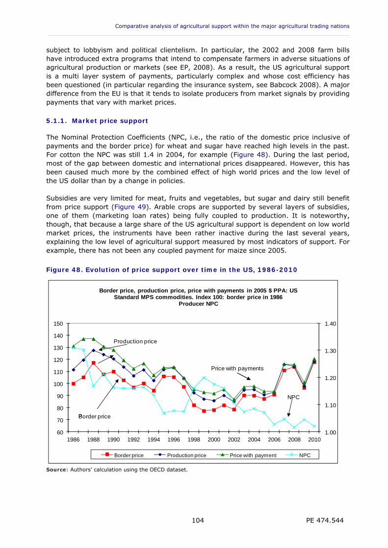
Comparative analysis of agricultural support within the major agricultural trading nations ___________________________________________________________________________________________
PE 474.544 104
subject to lobbyism and political clientelism. In particular, the 2002 and 2008 farm bills have introduced extra programs that intend to compensate farmers in adverse situations of agricultural production or markets (see EP, 2008). As a result, the US agricultural support is a multi layer system of payments, particularly complex and whose cost efficiency has been questioned (in particular regarding the insurance system, see Babcock 2008). A major difference from the EU is that it tends to isolate producers from market signals by providing payments that vary with market prices.
5.1.1. Market price support
The Nominal Protection Coefficients (NPC, i.e., the ratio of the domestic price inclusive of payments and the border price) for wheat and sugar have reached high levels in the past. For cotton the NPC was still 1.4 in 2004, for example (Figure 48). During the last period, most of the gap between domestic and international prices disappeared. However, this has been caused much more by the combined effect of high world prices and the low level of the US dollar than by a change in policies. Subsidies are very limited for meat, fruits and vegetables, but sugar and dairy still benefit from price support (Figure 49). Arable crops are supported by several layers of subsidies, one of them (marketing loan rates) being fully coupled to production. It is noteworthy, though, that because a large share of the US agricultural support is dependent on low world market prices, the instruments have been rather inactive during the last several years, explaining the low level of agricultural support measured by most indicators of support. For example, there has not been any coupled payment for maize since 2005. Figure 48. Evolution of price support over time in the US, 1986-2010
1.00
1.10
1.20
1.30
1.40
60
70
80
90
100
110
120
130
140
150
1986 1988 1990 1992 1994 1996 1998 2000 2002 2004 2006 2008 2010
Border price, production price, price with payments in 2005 $ PPA: USStandard MPS commodities. Index 100: border price in 1986
Producer NPC
Border price Production price Price with payment NPC
Border price
Price with payments
P
Production price
NPC
Source: Authors' calculation using the OECD dataset.
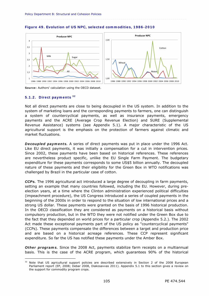
Policy Department B: Structural and Cohesion Policies _________________________________________________________________________________
PE 474.544 105
Figure 49. Evolution of US NPC, selected commodities, 1986-2010
1
1,5
2
2,5
3
3,5
4
1986 1988 1990 1992 1994 1996 1998 2000 2002 2004 2006 2008 2010
Producer NPC
SugarMilk
All
1,00
1,50
2,00
1986 1988 1990 1992 1994 1996 1998 2000 2002 2004 2006 2008 2010
Producer NPC
Cotton
Wheat
Maize
Source: Authors' calculation using the OECD dataset.
5.1.2. Direct payments 32
Not all direct payments are close to being decoupled in the US system. In addition to the system of marketing loans and the corresponding payments to farmers, one can distinguish a system of countercyclical payments, as well as insurance payments, emergency payments and the ACRE (Average Crop Revenue Election) and SURE (Supplemental Revenue Assistance) systems (see Appendix 5.1). A major characteristic of the US agricultural support is the emphasis on the protection of farmers against climatic and market fluctuations. Decoupled payments. A series of direct payments was put in place under the 1996 Act. Like EU direct payments, it was initially a compensation for a cut in intervention prices. Since 2002, these payments have been based on historical references. These references are nevertheless product specific, unlike the EU Single Farm Payment. The budgetary expenditure for these payments corresponds to some US$5 billion annually. The decoupled nature of these payments and their eligibility for the Green Box in WTO notifications was challenged by Brazil in the particular case of cotton. CCPs. The 1996 agricultural act introduced a large degree of decoupling in farm payments, setting an example that many countries followed, including the EU. However, during pre-election years, at a time where the Clinton administration experienced political difficulties (impeachment procedure), the US Congress introduced a series of coupled payments in the beginning of the 2000s in order to respond to the situation of low international prices and a strong US dollar. These payments were granted on the basis of 1996 historical production. In the OECD classification they are considered as payments on a historical basis without compulsory production, but in the WTO they were not notified under the Green Box due to the fact that they depended on world prices for a particular crop (Appendix 5.2.). The 2002 Act made these exceptional payments part of the US policy as "countercyclical payments" (CCPs). These payments compensate the differences between a target and production price and are based on a historical acreage references. These CCP represent significant expenditure. So far the US has notified these payments under the Amber Box. Other programs. Since the 2008 Act, payments stabilize farm receipts on a multiannual basis. This is the case of the ACRE program, which guarantees 90% of the historical
32 Note that US agricultural support policies are described extensively in Section 2 of the 2008 European
Parliament report (EP, 2008; Debar 2008, Diakosavvas 2011). Appendix 5.1 to this section gives a review on the support for commodity program crops.
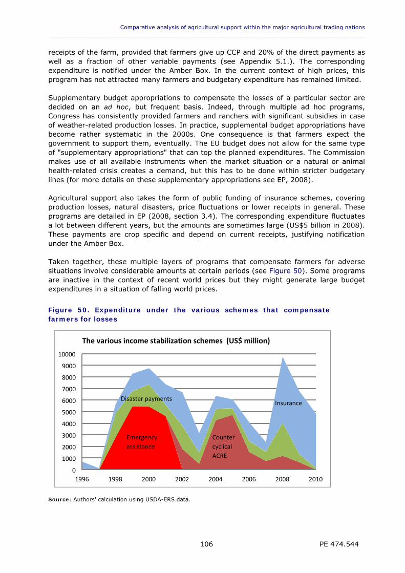
Comparative analysis of agricultural support within the major agricultural trading nations ___________________________________________________________________________________________
PE 474.544 106
receipts of the farm, provided that farmers give up CCP and 20% of the direct payments as well as a fraction of other variable payments (see Appendix 5.1.). The corresponding expenditure is notified under the Amber Box. In the current context of high prices, this program has not attracted many farmers and budgetary expenditure has remained limited. Supplementary budget appropriations to compensate the losses of a particular sector are decided on an ad hoc, but frequent basis. Indeed, through multiple ad hoc programs, Congress has consistently provided farmers and ranchers with significant subsidies in case of weather-related production losses. In practice, supplemental budget appropriations have become rather systematic in the 2000s. One consequence is that farmers expect the government to support them, eventually. The EU budget does not allow for the same type of "supplementary appropriations" that can top the planned expenditures. The Commission makes use of all available instruments when the market situation or a natural or animal health-related crisis creates a demand, but this has to be done within stricter budgetary lines (for more details on these supplementary appropriations see EP, 2008). Agricultural support also takes the form of public funding of insurance schemes, covering production losses, natural disasters, price fluctuations or lower receipts in general. These programs are detailed in EP (2008, section 3.4). The corresponding expenditure fluctuates a lot between different years, but the amounts are sometimes large (US$5 billion in 2008). These payments are crop specific and depend on current receipts, justifying notification under the Amber Box. Taken together, these multiple layers of programs that compensate farmers for adverse situations involve considerable amounts at certain periods (see Figure 50). Some programs are inactive in the context of recent world prices but they might generate large budget expenditures in a situation of falling world prices.
Figure 50. Expenditure under the various schemes that compensate farmers for losses
Source: Authors' calculation using USDA-ERS data.
0
1000
2000
3000
4000
5000
6000
7000
8000
9000
10000
1996 1998 2000 2002 2004 2006 2008 2010
The various income stabilization schemes (US$ million)
Emergency
assistance
Counter
cyclical
ACRE
InsuranceDisaster payments
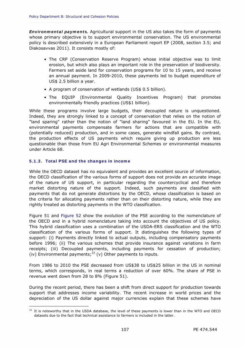
Policy Department B: Structural and Cohesion Policies _________________________________________________________________________________
PE 474.544 107
Environmental payments. Agricultural support in the US also takes the form of payments whose primary objective is to support environmental conservation. The US environmental policy is described extensively in a European Parliament report EP (2008, section 3.5; and Diakosavvas 2011). It consists mostly of:
• The CRP (Conservation Reserve Program) whose initial objective was to limit erosion, but which also plays an important role in the preservation of biodiversity. Farmers set aside land for conservation programs for 10 to 15 years, and receive an annual payment. In 2009-2010, these payments led to budget expenditure of US$ 2.5 billion a year.
• A program of conservation of wetlands (US$ 0.5 billion).
• The EQUIP (Environmental Quality Incentives Program) that promotes environmentally friendly practices (US$1 billion).
While these programs involve large budgets, their decoupled nature is unquestioned. Indeed, they are strongly linked to a concept of conservation that relies on the notion of "land sparing" rather than the notion of "land sharing" favoured in the EU. In the EU, environmental payments compensate farmers for actions that are compatible with (potentially reduced) production, and in some cases, generate windfall gains. By contrast, the production effects of US payments which require giving up production are less questionable than those from EU Agri Environmental Schemes or environmental measures under Article 68.
5.1.3. Total PSE and the changes in income
While the OECD dataset has no equivalent and provides an excellent source of information, the OECD classification of the various forms of support does not provide an accurate image of the nature of US support, in particular regarding the countercyclical and therefore market distorting nature of the support. Indeed, such payments are classified with payments that do not generate distortions by the OECD, whose classification is based on the criteria for allocating payments rather than on their distorting nature, while they are rightly treated as distorting payments in the WTO classification. Figure 51 and Figure 52 show the evolution of the PSE according to the nomenclature of the OECD and in a hybrid nomenclature taking into account the objectives of US policy. This hybrid classification uses a combination of the USDA-ERS classification and the WTO classification of the various forms of support. It distinguishes the following types of support: (i) Payments directly linked to actual outputs, including compensatory payments before 1996; (ii) The various schemes that provide insurance against variations in farm receipts; (iii) Decoupled payments, including payments for cessation of production; (iv) Environmental payments;33 (v) Other payments to inputs. From 1986 to 2010 the PSE decreased from US$38 to US$25 billion in the US in nominal terms, which corresponds, in real terms a reduction of over 60%. The share of PSE in revenue went down from 28 to 8% (Figure 51). During the recent period, there has been a shift from direct support for production towards support that addresses income variability. The recent increase in world prices and the depreciation of the US dollar against major currencies explain that these schemes have
33 It is noteworthy that in the USDA database, the level of these payments is lower than in the WTO and OECD
datasets due to the fact that technical assistance to farmers is included in the latter.
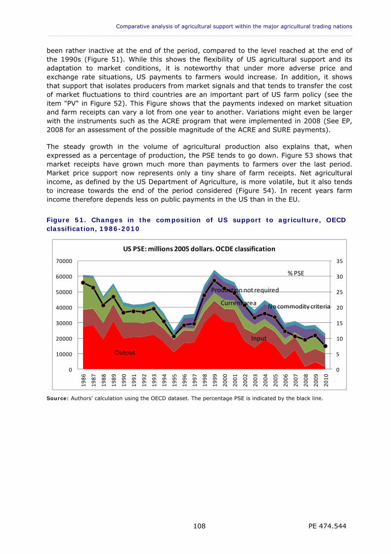
Comparative analysis of agricultural support within the major agricultural trading nations ___________________________________________________________________________________________
PE 474.544 108
been rather inactive at the end of the period, compared to the level reached at the end of the 1990s (Figure 51). While this shows the flexibility of US agricultural support and its adaptation to market conditions, it is noteworthy that under more adverse price and exchange rate situations, US payments to farmers would increase. In addition, it shows that support that isolates producers from market signals and that tends to transfer the cost of market fluctuations to third countries are an important part of US farm policy (see the item "PV" in Figure 52). This Figure shows that the payments indexed on market situation and farm receipts can vary a lot from one year to another. Variations might even be larger with the instruments such as the ACRE program that were implemented in 2008 (See EP, 2008 for an assessment of the possible magnitude of the ACRE and SURE payments). The steady growth in the volume of agricultural production also explains that, when expressed as a percentage of production, the PSE tends to go down. Figure 53 shows that market receipts have grown much more than payments to farmers over the last period. Market price support now represents only a tiny share of farm receipts. Net agricultural income, as defined by the US Department of Agriculture, is more volatile, but it also tends to increase towards the end of the period considered (Figure 54). In recent years farm income therefore depends less on public payments in the US than in the EU.
Figure 51. Changes in the composition of US support to agriculture, OECD classification, 1986-2010
0
5
10
15
20
25
30
35
0
10000
20000
30000
40000
50000
60000
70000
1986
1987
1988
1989
1990
1991
1992
1993
1994
1995
1996
1997
1998
1999
2000
2001
2002
2003
2004
2005
2006
2007
2008
2009
2010
US PSE: millions 2005 dollars. OCDE classification
Output
Input
Current area
Production not required
% PSE
No commodity criteria
Source: Authors' calculation using the OECD dataset. The percentage PSE is indicated by the black line.
Policy Department B: Structural and Cohesion Policies _________________________________________________________________________________
PE 474.544 109
Figure 52.Changes in the composition of US support to agriculture, 1986-2010
0
10000
20000
30000
40000
50000
60000
70000
1986
1987
1988
1989
1990
1991
1992
1993
1994
1995
1996
1997
1998
1999
2000
2001
2002
2003
2004
2005
2006
2007
2008
2009
2010
US PSE: millions 2005 dollars. Hybrid classification
MPS
PO + DFPPO + DFP
Other
Other
PVDP
EP
Source: Authors' calculation using the OECD dataset. PO + DFP: payment on output and deficiency payments before 1996. PV: payments indexed on market situation and farm receipts. DP: decoupled payments. EP: environment payments.
Figure 53. Farm receipts and the level of the US PSE, 1986-2010
0
100
200
300
400
1986 1988 1990 1992 1994 1996 1998 2000 2002 2004 2006 2008 2010
Farm receipt, MPS and other PSE (US: billion dollars 2005)
MPSOther PSE
Receipts ‐ ESP
Receipts
Source: Authors' calculation using the OECD dataset.
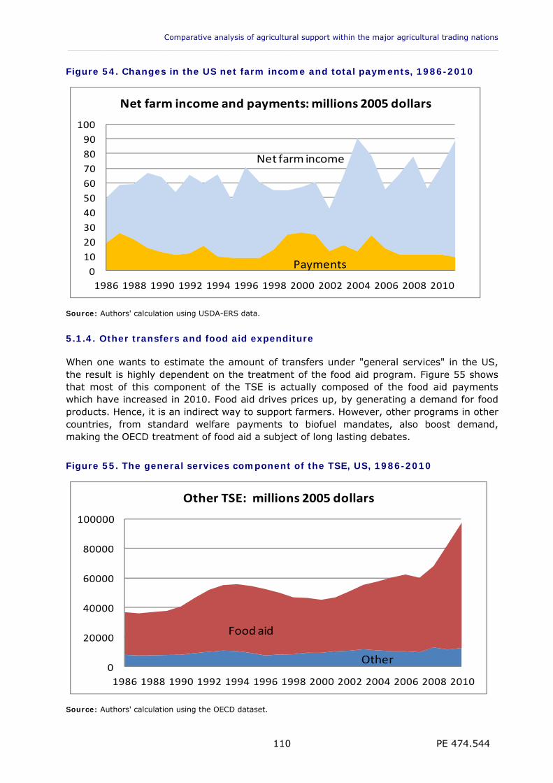
Comparative analysis of agricultural support within the major agricultural trading nations ___________________________________________________________________________________________
PE 474.544 110
Figure 54. Changes in the US net farm income and total payments, 1986-2010
0
10
20
30
40
50
60
70
80
90
100
1986 1988 1990 1992 1994 1996 1998 2000 2002 2004 2006 2008 2010
Net farm income and payments: millions 2005 dollars
Payments
Net farm income
Source: Authors' calculation using USDA-ERS data.
5.1.4. Other transfers and food aid expenditure
When one wants to estimate the amount of transfers under "general services" in the US, the result is highly dependent on the treatment of the food aid program. Figure 55 shows that most of this component of the TSE is actually composed of the food aid payments which have increased in 2010. Food aid drives prices up, by generating a demand for food products. Hence, it is an indirect way to support farmers. However, other programs in other countries, from standard welfare payments to biofuel mandates, also boost demand, making the OECD treatment of food aid a subject of long lasting debates.
Figure 55. The general services component of the TSE, US, 1986-2010
0
20000
40000
60000
80000
100000
1986 1988 1990 1992 1994 1996 1998 2000 2002 2004 2006 2008 2010
Other TSE: millions 2005 dollars
Food aid
Other
Source: Authors' calculation using the OECD dataset.
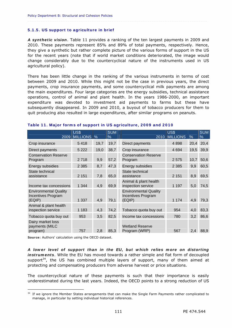
Policy Department B: Structural and Cohesion Policies _________________________________________________________________________________
PE 474.544 111
5.1.5. US support to agriculture in brief
A synthetic vision. Table 11 provides a ranking of the ten largest payments in 2009 and 2010. These payments represent 85% and 89% of total payments, respectively. Hence, they give a synthetic but rather complete picture of the various forms of support in the US for the recent years (note that if world market conditions deteriorated, the image would change considerably due to the countercyclical nature of the instruments used in US agricultural policy). There has been little change in the ranking of the various instruments in terms of cost between 2009 and 2010. While this might not be the case in previous years, the direct payments, crop insurance payments, and some countercyclical milk payments are among the main expenditures. Four large categories are the energy subsidies, technical assistance operations, control of animal and plant health. In the years 1986-2000, an important expenditure was devoted to investment aid payments to farms but these have subsequently disappeared. In 2009 and 2010, a buyout of tobacco producers for them to quit producing also resulted in large expenditures, after similar programs on peanuts.
Table 11. Major forms of support in US agriculture, 2009 and 2010
2009US$ MILLIONS %
SUM % 2010
US$ MILLIONS %
SUM %
Crop insurance 5 418 19,7 19,7 Direct payments 4 898 20,4 20,4
Direct payments 5 222 19,0 38,7 Crop insurance 4 694 19,5 39,9Conservation Reserve Program 2 718 9,9 57,2
Conservation Reserve Program 2 575 10,7 50,6
Energy subsidies 2 385 8,7 47,3 Energy subsidies 2 385 9,9 60,5State technical assistance 2 151 7,8 65,0
State technical assistance 2 151 8,9 69,5
Income tax concessions 1 344 4,9 69,9Animal & plant health inspection service 1 197 5,0 74,5
Environmental Quality Incentives Program (EQIP) 1 337 4,9 79,1
Environmental Quality Incentives Program (EQIP) 1 174 4,9 79,3
Animal & plant health inspection service 1 183 4,3 74,2 Tobacco quota buy out 954 4,0 83,3
Tobacco quota buy out 953 3,5 82,5 Income tax concessions 780 3,2 86,6Dairy market loss payments (MILC program) 757 2,8 85,3
Wetland Reserve Program (WRP) 567 2,4 88,9
Source: Authors' calculation using the OECD dataset.
A lower level of support than in the EU, but which relies more on distorting instruments. While the EU has moved towards a rather simple and flat form of decoupled support34, the US has combined multiple layers of support, many of them aimed at protecting and compensating producers from adverse harvest or price situations. The countercyclical nature of these payments is such that their importance is easily underestimated during the last years. Indeed, the OECD points to a strong reduction of US
34 If we ignore the Member States arrangements that can make the Single Farm Payments rather complicated to
manage, in particular by setting individual historical references.
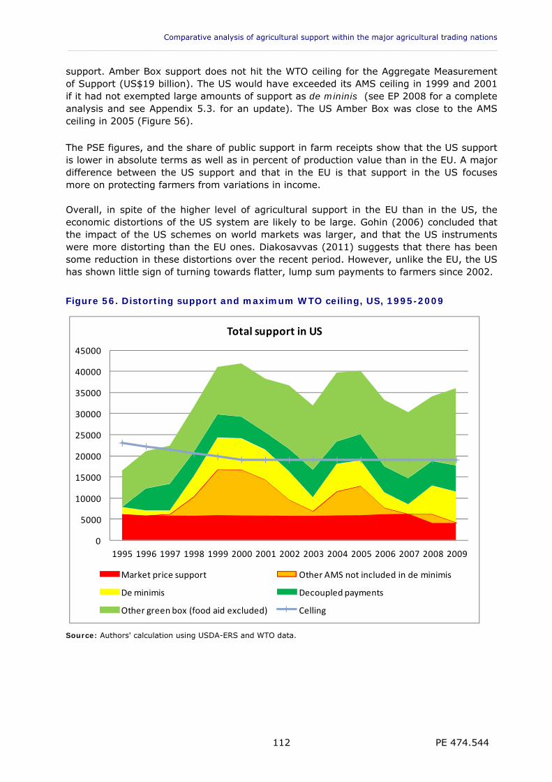
Comparative analysis of agricultural support within the major agricultural trading nations ___________________________________________________________________________________________
PE 474.544 112
support. Amber Box support does not hit the WTO ceiling for the Aggregate Measurement of Support (US$19 billion). The US would have exceeded its AMS ceiling in 1999 and 2001 if it had not exempted large amounts of support as de mininis (see EP 2008 for a complete analysis and see Appendix 5.3. for an update). The US Amber Box was close to the AMS ceiling in 2005 (Figure 56). The PSE figures, and the share of public support in farm receipts show that the US support is lower in absolute terms as well as in percent of production value than in the EU. A major difference between the US support and that in the EU is that support in the US focuses more on protecting farmers from variations in income. Overall, in spite of the higher level of agricultural support in the EU than in the US, the economic distortions of the US system are likely to be large. Gohin (2006) concluded that the impact of the US schemes on world markets was larger, and that the US instruments were more distorting than the EU ones. Diakosavvas (2011) suggests that there has been some reduction in these distortions over the recent period. However, unlike the EU, the US has shown little sign of turning towards flatter, lump sum payments to farmers since 2002.
Figure 56. Distorting support and maximum WTO ceiling, US, 1995-2009
0
5000
10000
15000
20000
25000
30000
35000
40000
45000
1995 1996 1997 1998 1999 2000 2001 2002 2003 2004 2005 2006 2007 2008 2009
Total support in US
Market price support Other AMS not included in de minimis
De minimis Decoupled payments
Other green box (food aid excluded) Celling
Source: Authors' calculation using USDA-ERS and WTO data.
Policy Department B: Structural and Cohesion Policies _________________________________________________________________________________
PE 474.544 113
5.2. Agricultural support in Canada
Canada is a major agricultural exporter. In the WTO framework, as one of the "Cairns group"' countries, Canada has argued for liberalization of agricultural markets. This does not mean that there is no agricultural support in Canada. High tariffs and some public intervention protect and support particular sectors such as dairy and, to a lesser extent, poultry. State trading entities, such as marketing boards, still contribute to market regulation, although the Canadian government is targeting 1 August 2012 for removing the mandatory requirement for western producers to market wheat and barley through the Canadian Wheat Board (some legal challenges may affect the actual date). Price support and transportation subsidies were removed in the 1990s (see Skogstad 2011 for details). The main orientations of Canadian agricultural policy are defined every five years by the federal and provincial governments. The most recent framework of strategic orientations was defined for the 2008-2013 period. The various Canadian provinces have a large degree of latitude to define specific measures. The largest share of public expenditure for agriculture goes to income stabilisation and support to investment. A difference from the US is that a significant share of countercyclical support is notified under the Green Box in the WTO as meeting the criteria of income safety net programmes. The gap between domestic and world prices has progressively been reduced since 1986. The reason is less the high level of world prices during the recent period than the reforms that have taken place in the 1990s. The NPC, i.e., the ratio between the average price received by producers at the farm gate (including payments per current output), and the border price has gone down. It was 1.45 in 1986 and only 1.17 in 1996. It reached 1.02 in 2007 (Figure 57). This gap went up, however, in 2009 when world prices went down. Because support to crops was largely dismantled already in the 1990s, the remaining price support that explains the NPC is caused by the system of guaranteed prices and quotas in the dairy sector. The transportation subsidies for Western grains and oilseed, which had their origin in regional economic development decisions dating back as far as the 1890s, represented a a large component of the PSE (Figure 58). The 1995 discontinuation of these subsidies had a significant impact on agricultural support measured by the OECD. The cut in transportation subsidies was eased by a temporary direct payment notified as decoupled support in the WTO Green Box (Figure 59). Dairy production quotas are managed by each Province. The supported price for milk relies on a high tariff protection and strict import quotas. Supply control has also persisted for poultry and eggs. Overall, support to agricultural products (i.e., coupled support) remained stable in the 2000s, except in situations of high world prices where it went down. Three quarters of the total support correspond to dairy (Figure 59). It is noteworthy, though that the system of production quotas is such that it limits the expansion of the main supported commodity, hence limiting the distortions in world markets and the externalities for third countries. The real PSE, expressed in constant 2005 Canadian dollars reaches C$6.9 billion in 2010. The percentage PSE is 17% when expressed as a ratio to the value of production. As much as 12 percentage points correspond to single commodity transfers, mostly to dairy. Part of the non commodity specific support is based on current area or number of animals, and is therefore rather distorting compared to payments of a more lump character (Figure 60).
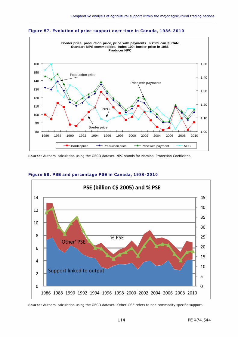
Comparative analysis of agricultural support within the major agricultural trading nations ___________________________________________________________________________________________
PE 474.544 114
Figure 57. Evolution of price support over time in Canada, 1986-2010
1,00
1,10
1,20
1,30
1,40
1,50
80
90
100
110
120
130
140
150
160
1986 1988 1990 1992 1994 1996 1998 2000 2002 2004 2006 2008 2010
Border price, production price, price with payments in 2005 can $: CANStandart MPS commodities. Index 100: border price in 1986
Producer NPC
Border price Production price Price with payment NPC
Border price
Price with payments
Production price
NPC
Source: Authors' calculation using the OECD dataset. NPC stands for Nominal Protection Coefficient.
Figure 58. PSE and percentage PSE in Canada, 1986-2010
Source: Authors' calculation using the OECD dataset. 'Other' PSE refers to non commodity specific support.
0
5
10
15
20
25
30
35
40
45
0
2
4
6
8
10
12
14
1986 1988 1990 1992 1994 1996 1998 2000 2002 2004 2006 2008 2010
PSE (billion C$ 2005) and % PSE
Support linked to output
'Other' PSE % PSE
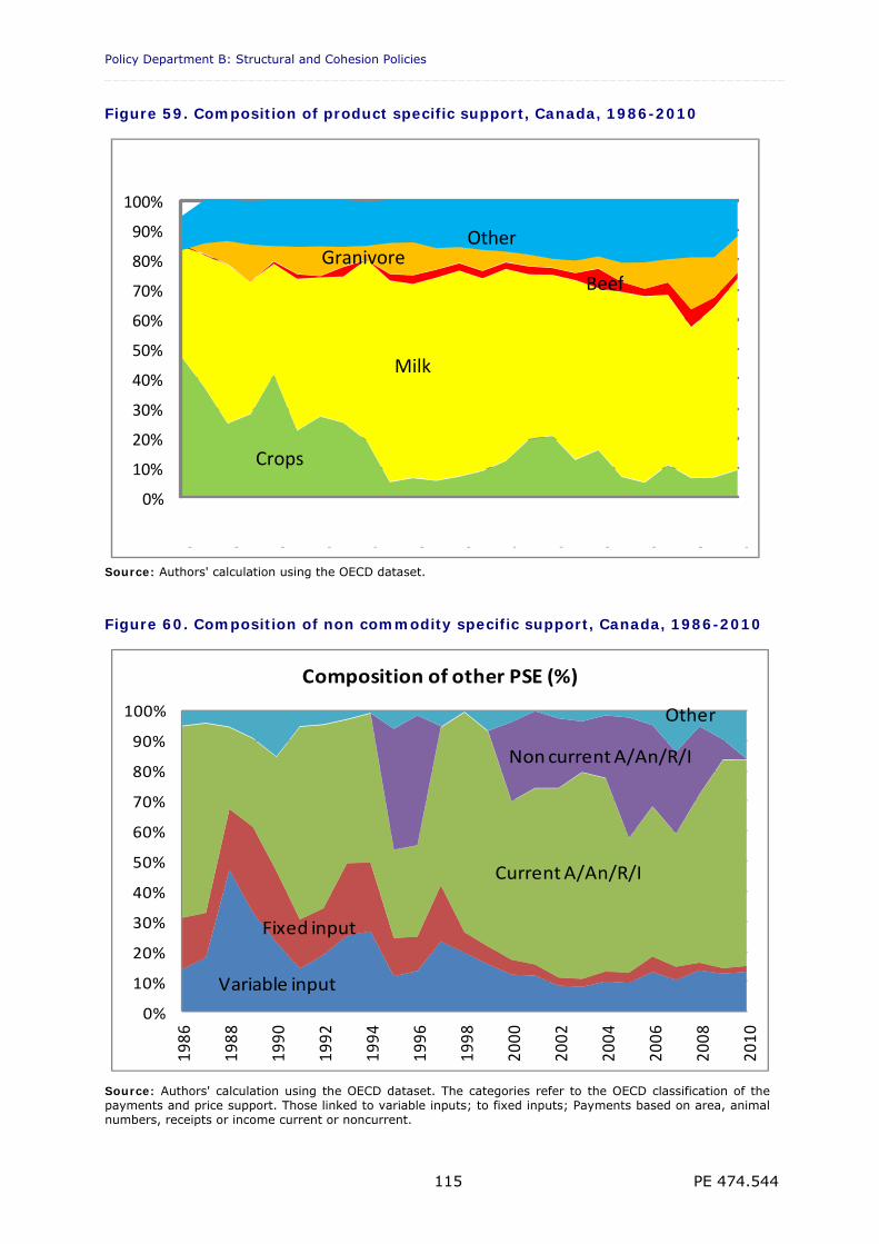
Policy Department B: Structural and Cohesion Policies _________________________________________________________________________________
PE 474.544 115
Figure 59. Composition of product specific support, Canada, 1986-2010
Source: Authors' calculation using the OECD dataset.
Figure 60. Composition of non commodity specific support, Canada, 1986-2010
0%
10%
20%
30%
40%
50%
60%
70%
80%
90%
100%
1986
1988
1990
1992
1994
1996
1998
2000
2002
2004
2006
2008
2010
Composition of other PSE (%)
Variable input
Fixed input
Current A/An/R/I
Non current A/An/R/I
Other
Source: Authors' calculation using the OECD dataset. The categories refer to the OECD classification of the payments and price support. Those linked to variable inputs; to fixed inputs; Payments based on area, animal numbers, receipts or income current or noncurrent.
0%
10%
20%
30%
40%
50%
60%
70%
80%
90%
100%
1986 1988 1990 1992 1994 1996 1998 2000 2002 2004 2006 2008 2010
Crops
Milk
Beef
Granivore Other
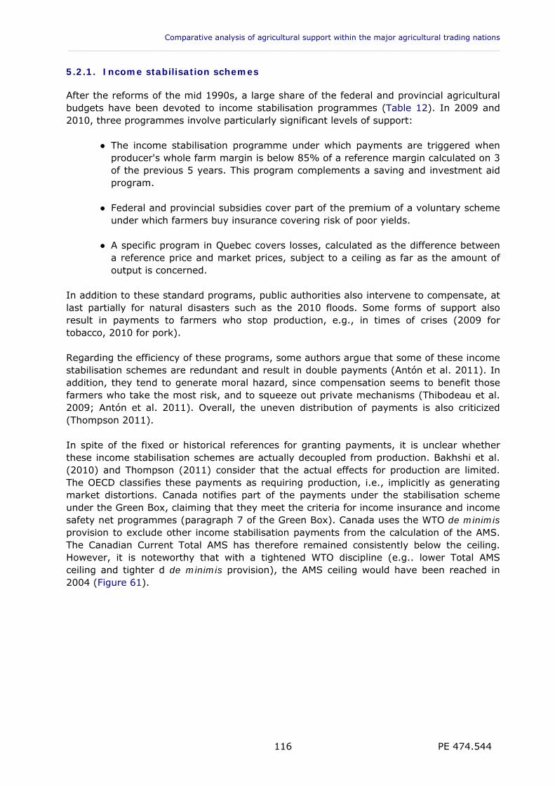
Comparative analysis of agricultural support within the major agricultural trading nations ___________________________________________________________________________________________
PE 474.544 116
5.2.1. Income stabilisation schemes
After the reforms of the mid 1990s, a large share of the federal and provincial agricultural budgets have been devoted to income stabilisation programmes (Table 12). In 2009 and 2010, three programmes involve particularly significant levels of support:
● The income stabilisation programme under which payments are triggered when producer's whole farm margin is below 85% of a reference margin calculated on 3 of the previous 5 years. This program complements a saving and investment aid program.
● Federal and provincial subsidies cover part of the premium of a voluntary scheme
under which farmers buy insurance covering risk of poor yields. ● A specific program in Quebec covers losses, calculated as the difference between
a reference price and market prices, subject to a ceiling as far as the amount of output is concerned.
In addition to these standard programs, public authorities also intervene to compensate, at last partially for natural disasters such as the 2010 floods. Some forms of support also result in payments to farmers who stop production, e.g., in times of crises (2009 for tobacco, 2010 for pork). Regarding the efficiency of these programs, some authors argue that some of these income stabilisation schemes are redundant and result in double payments (Antón et al. 2011). In addition, they tend to generate moral hazard, since compensation seems to benefit those farmers who take the most risk, and to squeeze out private mechanisms (Thibodeau et al. 2009; Antón et al. 2011). Overall, the uneven distribution of payments is also criticized (Thompson 2011). In spite of the fixed or historical references for granting payments, it is unclear whether these income stabilisation schemes are actually decoupled from production. Bakhshi et al. (2010) and Thompson (2011) consider that the actual effects for production are limited. The OECD classifies these payments as requiring production, i.e., implicitly as generating market distortions. Canada notifies part of the payments under the stabilisation scheme under the Green Box, claiming that they meet the criteria for income insurance and income safety net programmes (paragraph 7 of the Green Box). Canada uses the WTO de minimis provision to exclude other income stabilisation payments from the calculation of the AMS. The Canadian Current Total AMS has therefore remained consistently below the ceiling. However, it is noteworthy that with a tightened WTO discipline (e.g.. lower Total AMS ceiling and tighter d de minimis provision), the AMS ceiling would have been reached in 2004 (Figure 61).
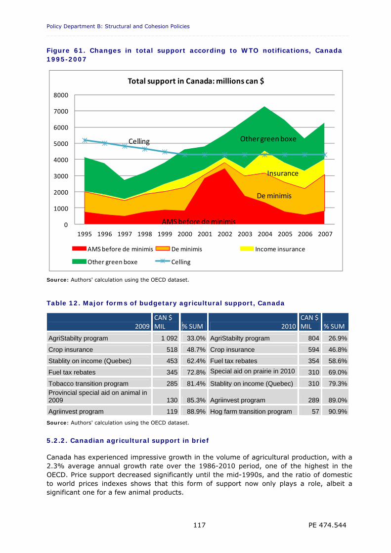
Policy Department B: Structural and Cohesion Policies _________________________________________________________________________________
PE 474.544 117
Figure 61. Changes in total support according to WTO notifications, Canada 1995-2007
0
1000
2000
3000
4000
5000
6000
7000
8000
1995 1996 1997 1998 1999 2000 2001 2002 2003 2004 2005 2006 2007
Total support in Canada: millions can $
AMS before de minimis De minimis Income insurance
Other green boxe Celling
AMS before de minimis
Insurance
De minimis
Other green boxeCelling
Source: Authors' calculation using the OECD dataset.
Table 12. Major forms of budgetary agricultural support, Canada
2009 CAN $ MIL % SUM 2010
CAN $ MIL % SUM
AgriStabilty program 1 092 33.0% AgriStabilty program 804 26.9%
Crop insurance 518 48.7% Crop insurance 594 46.8%
Stablity on income (Quebec) 453 62.4% Fuel tax rebates 354 58.6%
Fuel tax rebates 345 72.8% Special aid on prairie in 2010 310 69.0%
Tobacco transition program 285 81.4% Stablity on income (Quebec) 310 79.3%Provincial special aid on animal in 2009 130 85.3% Agriinvest program 289 89.0%
Agriinvest program 119 88.9% Hog farm transition program 57 90.9%
Source: Authors' calculation using the OECD dataset.
5.2.2. Canadian agricultural support in brief
Canada has experienced impressive growth in the volume of agricultural production, with a 2.3% average annual growth rate over the 1986-2010 period, one of the highest in the OECD. Price support decreased significantly until the mid-1990s, and the ratio of domestic to world prices indexes shows that this form of support now only plays a role, albeit a significant one for a few animal products.
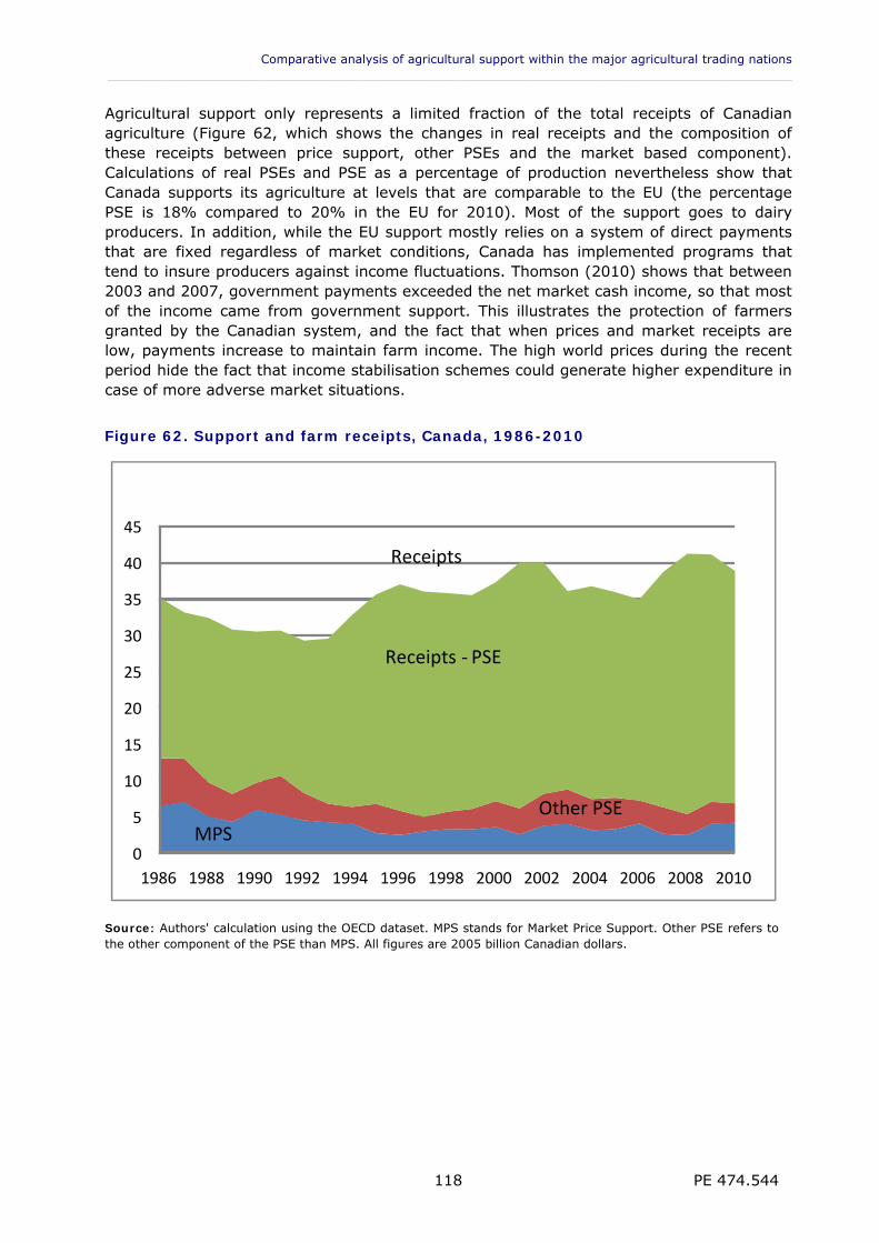
Comparative analysis of agricultural support within the major agricultural trading nations ___________________________________________________________________________________________
PE 474.544 118
Agricultural support only represents a limited fraction of the total receipts of Canadian agriculture (Figure 62, which shows the changes in real receipts and the composition of these receipts between price support, other PSEs and the market based component). Calculations of real PSEs and PSE as a percentage of production nevertheless show that Canada supports its agriculture at levels that are comparable to the EU (the percentage PSE is 18% compared to 20% in the EU for 2010). Most of the support goes to dairy producers. In addition, while the EU support mostly relies on a system of direct payments that are fixed regardless of market conditions, Canada has implemented programs that tend to insure producers against income fluctuations. Thomson (2010) shows that between 2003 and 2007, government payments exceeded the net market cash income, so that most of the income came from government support. This illustrates the protection of farmers granted by the Canadian system, and the fact that when prices and market receipts are low, payments increase to maintain farm income. The high world prices during the recent period hide the fact that income stabilisation schemes could generate higher expenditure in case of more adverse market situations.
Figure 62. Support and farm receipts, Canada, 1986-2010
Source: Authors' calculation using the OECD dataset. MPS stands for Market Price Support. Other PSE refers to the other component of the PSE than MPS. All figures are 2005 billion Canadian dollars.
0
5
10
15
20
25
30
35
40
45
1986 1988 1990 1992 1994 1996 1998 2000 2002 2004 2006 2008 2010
MPS
Other PSE
Receipts ‐ PSE
Receipts
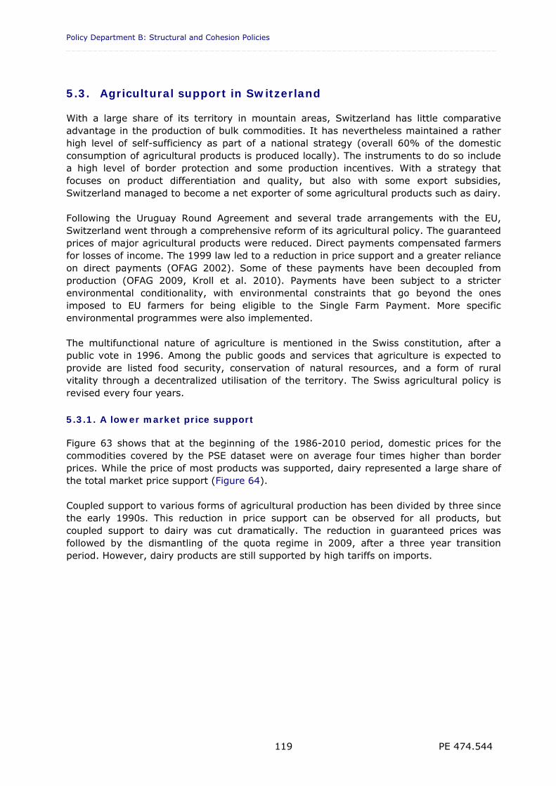
Policy Department B: Structural and Cohesion Policies _________________________________________________________________________________
PE 474.544 119
5.3. Agricultural support in Switzerland
With a large share of its territory in mountain areas, Switzerland has little comparative advantage in the production of bulk commodities. It has nevertheless maintained a rather high level of self-sufficiency as part of a national strategy (overall 60% of the domestic consumption of agricultural products is produced locally). The instruments to do so include a high level of border protection and some production incentives. With a strategy that focuses on product differentiation and quality, but also with some export subsidies, Switzerland managed to become a net exporter of some agricultural products such as dairy. Following the Uruguay Round Agreement and several trade arrangements with the EU, Switzerland went through a comprehensive reform of its agricultural policy. The guaranteed prices of major agricultural products were reduced. Direct payments compensated farmers for losses of income. The 1999 law led to a reduction in price support and a greater reliance on direct payments (OFAG 2002). Some of these payments have been decoupled from production (OFAG 2009, Kroll et al. 2010). Payments have been subject to a stricter environmental conditionality, with environmental constraints that go beyond the ones imposed to EU farmers for being eligible to the Single Farm Payment. More specific environmental programmes were also implemented. The multifunctional nature of agriculture is mentioned in the Swiss constitution, after a public vote in 1996. Among the public goods and services that agriculture is expected to provide are listed food security, conservation of natural resources, and a form of rural vitality through a decentralized utilisation of the territory. The Swiss agricultural policy is revised every four years.
5.3.1. A lower market price support
Figure 63 shows that at the beginning of the 1986-2010 period, domestic prices for the commodities covered by the PSE dataset were on average four times higher than border prices. While the price of most products was supported, dairy represented a large share of the total market price support (Figure 64). Coupled support to various forms of agricultural production has been divided by three since the early 1990s. This reduction in price support can be observed for all products, but coupled support to dairy was cut dramatically. The reduction in guaranteed prices was followed by the dismantling of the quota regime in 2009, after a three year transition period. However, dairy products are still supported by high tariffs on imports.
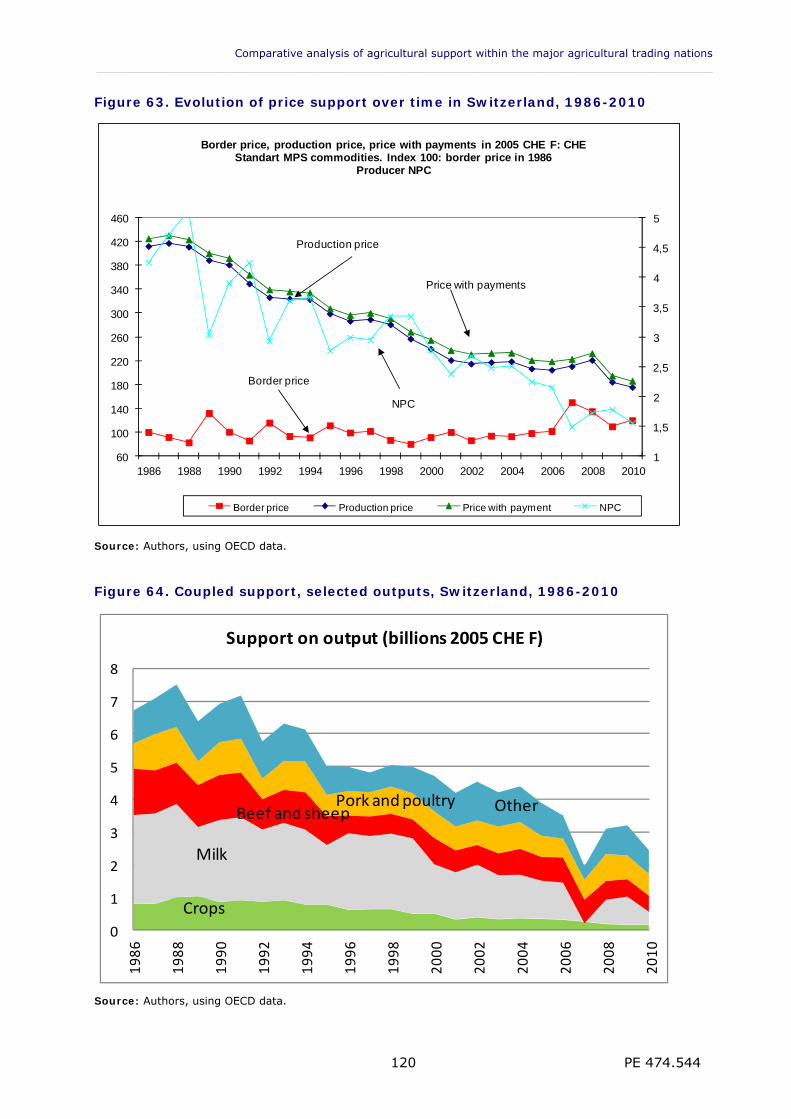
Comparative analysis of agricultural support within the major agricultural trading nations ___________________________________________________________________________________________
PE 474.544 120
Figure 63. Evolution of price support over time in Switzerland, 1986-2010
1
1,5
2
2,5
3
3,5
4
4,5
5
60
100
140
180
220
260
300
340
380
420
460
1986 1988 1990 1992 1994 1996 1998 2000 2002 2004 2006 2008 2010
Border price, production price, price with payments in 2005 CHE F: CHEStandart MPS commodities. Index 100: border price in 1986
Producer NPC
Border price Production price Price with payment NPC
Border price
Price with payments
Production price
NPC
Source: Authors, using OECD data.
Figure 64. Coupled support, selected outputs, Switzerland, 1986-2010
0
1
2
3
4
5
6
7
8
1986
1988
1990
1992
1994
1996
1998
2000
2002
2004
2006
2008
2010
Support on output (billions 2005 CHE F)
Crops
Milk
Beef and sheepPork and poultry Other
Source: Authors, using OECD data.
Policy Department B: Structural and Cohesion Policies _________________________________________________________________________________
PE 474.544 121
5.3.2. Direct payments and the need to deliver public goods
A distinction is made between general and ecological direct payments. General direct payments are compensation for the basic tasks, as set out in the constitution, of ensuring food supplies, maintaining the landscape and helping to preserve social structures in rural areas. They include an area payment and one for grazing animals. The area payment is granted independent of any requirement to produce particular crops. Payments are subject to an income and asset ceiling and are differentiated by farm size. In upland and mountain areas additional payments are provided to compensate for difficult farming conditions. Eligibility for the general direct payment is dependent on farmers proving that they comply with a set of minimum rules; the so-called “proof of ecological performance” (Prestations écologiques requises – PER). The key elements of proof of ecological performance are an appropriate proportion of ecological compensation areas, rational use of fertilisers, crop rotation, soil protection, economic and specific use of plant treatment products and animal welfare measures. In addition to the general direct payment system, farmers can also enroll in a voluntary agri-environment scheme which remunerates particular services separately through ecological direct payments. Among other things, the farmer receives additional payment for extensive meadow-land, reed-beds, natural field margins, permanent flowery meadows and rotated fallow fields, hedges, copses and wooded river banks and standard fruit trees. Farmers who wish to increase their ecological compensation areas beyond the minimum 7% required for cross-compliance receive additional payments under this scheme. Organic farming is also subsidised. In the OECD dataset, a decrease in environmental payments is observed in 1999, while payments with compulsory conditions increase. This reflects the shift from voluntary measures to cross compliance of the direct payments to environmental conditions. Nowadays, all direct payments are conditional on the "proof of ecological performance". This means that direct payments are only granted if farmers meet a number of environmental conditions. These conditions appear more stringent than the conditionality on a set of directives and good agricultural and environmental conditions in the EU. Ecological compensation, one of the requirements for general direct payments, involves that a farm can chose between 17 types of compensatory areas (e.g., low intensity meadows, extensive pasture, buffer strips, hedges, traditional orchards, wetlands, set aside land, etc.). Farmers must devote at least 7% of the agricultural area to such uses that promote natural or semi natural habitats, farmed in an extensive manner, or left to include characteristic elements of rural landscape (dry stone walls, isolated trees, etc.). The implementation of ecological compensation areas intends to preserve or create some natural or semi natural areas, maintain and develop diversity of flora and fauna on agricultural areas, maintain typical elements of the rural landscape, and protect natural resources (interdiction of fertilizer and pesticides on ecological compensation areas). The results of this policy in terms of biodiversity are quoted as one of the few successes in Europe (see section 6.2.3). Ecological direct payments represent 20% of direct payments in 2010, according to the Swiss Ministry of agriculture. These payments are paid to farmers willing to implement even more stringent agricultural practices with regard to environmental standards. In 2010, they included schemes for extensive livestock production respectful of animal welfare (40%

Comparative analysis of agricultural support within the major agricultural trading nations ___________________________________________________________________________________________
PE 474.544 122
of payments, requiring that animals be taken out regularly, and grazed in the summertime), 20% to extra ecological compensation (extensive meadows, hedges). If one accounts for other environmental programmes that complement the requirement of ecological compensation for obtaining the direct payments, surfaces devoted to such an ecological focus account for an impressive 145 000 ha i.e., 13.6% of Swiss agricultural area (Trometter et al., 2008).
5.3.3. A decrease in support as well as farm income
When expressed in real value, the Swiss PSE has decreased by half since 1986. However, because of the shift from consumer based support to taxpayer based support, prices have gone down. The share of the PSE in total receipts is nevertheless close to 50% in 2010. Direct payments have only partially compensated the decrease in producer prices. In real values, farm receipts have decreased by a third since 1986 (Figure 66). According to the macroeconomic accounts, the net income in the agricultural branch has decreased by half between 1986 and 2000 (Figure 67). Since 2000, both subsidies and incomes expressed in real values have remained stable. Currently agricultural subsidies account for roughly 100% of the net farm income.
Figure 65. Evolution of PSE, Switzerland, 1986-2010
Source: Authors, using OECD data and PPP data.
0
10
20
30
40
50
60
70
80
90
0
2
4
6
8
10
12
1986 1988 1990 1992 1994 1996 1998 2000 2002 2004 2006 2008 2010
PSE (billion 2005 CHF) and % PSE
Support on output
Other PSE
% PSE
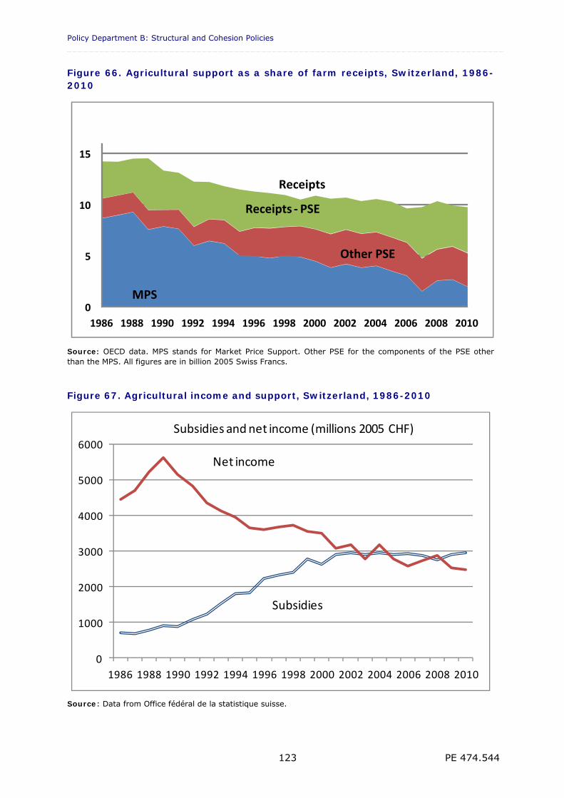
Policy Department B: Structural and Cohesion Policies _________________________________________________________________________________
PE 474.544 123
Figure 66. Agricultural support as a share of farm receipts, Switzerland, 1986-2010
Source: OECD data. MPS stands for Market Price Support. Other PSE for the components of the PSE other than the MPS. All figures are in billion 2005 Swiss Francs.
Figure 67. Agricultural income and support, Switzerland, 1986-2010
0
1000
2000
3000
4000
5000
6000
1986 1988 1990 1992 1994 1996 1998 2000 2002 2004 2006 2008 2010
Subsidies and net income (millions 2005 CHF)
Net income
Subsidies
Source: Data from Office fédéral de la statistique suisse.
0
5
10
15
1986 1988 1990 1992 1994 1996 1998 2000 2002 2004 2006 2008 2010
MPS
Other PSE
Receipts ‐ PSE
Receipts
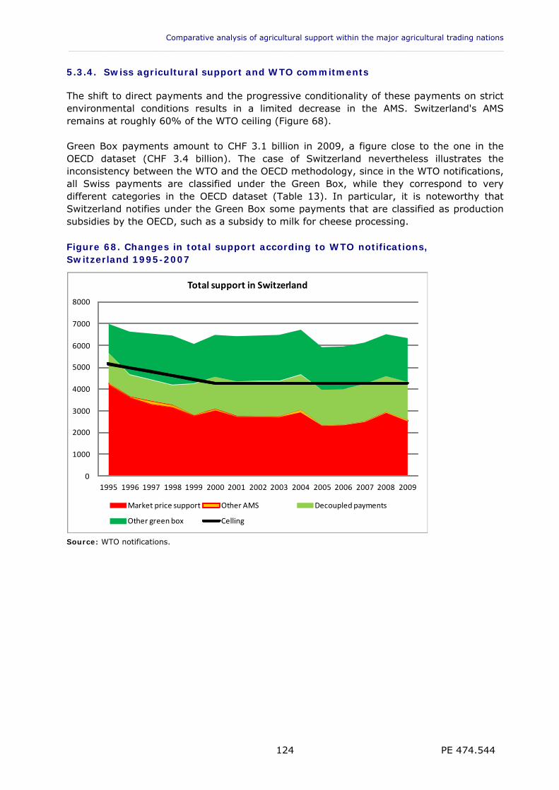
Comparative analysis of agricultural support within the major agricultural trading nations ___________________________________________________________________________________________
PE 474.544 124
5.3.4. Swiss agricultural support and WTO commitments
The shift to direct payments and the progressive conditionality of these payments on strict environmental conditions results in a limited decrease in the AMS. Switzerland's AMS remains at roughly 60% of the WTO ceiling (Figure 68). Green Box payments amount to CHF 3.1 billion in 2009, a figure close to the one in the OECD dataset (CHF 3.4 billion). The case of Switzerland nevertheless illustrates the inconsistency between the WTO and the OECD methodology, since in the WTO notifications, all Swiss payments are classified under the Green Box, while they correspond to very different categories in the OECD dataset (Table 13). In particular, it is noteworthy that Switzerland notifies under the Green Box some payments that are classified as production subsidies by the OECD, such as a subsidy to milk for cheese processing. Figure 68. Changes in total support according to WTO notifications, Switzerland 1995-2007
0
1000
2000
3000
4000
5000
6000
7000
8000
1995 1996 1997 1998 1999 2000 2001 2002 2003 2004 2005 2006 2007 2008 2009
Total support in Switzerland
Market price support Other AMS Decoupled payments
Other green box Celling
Source: WTO notifications.
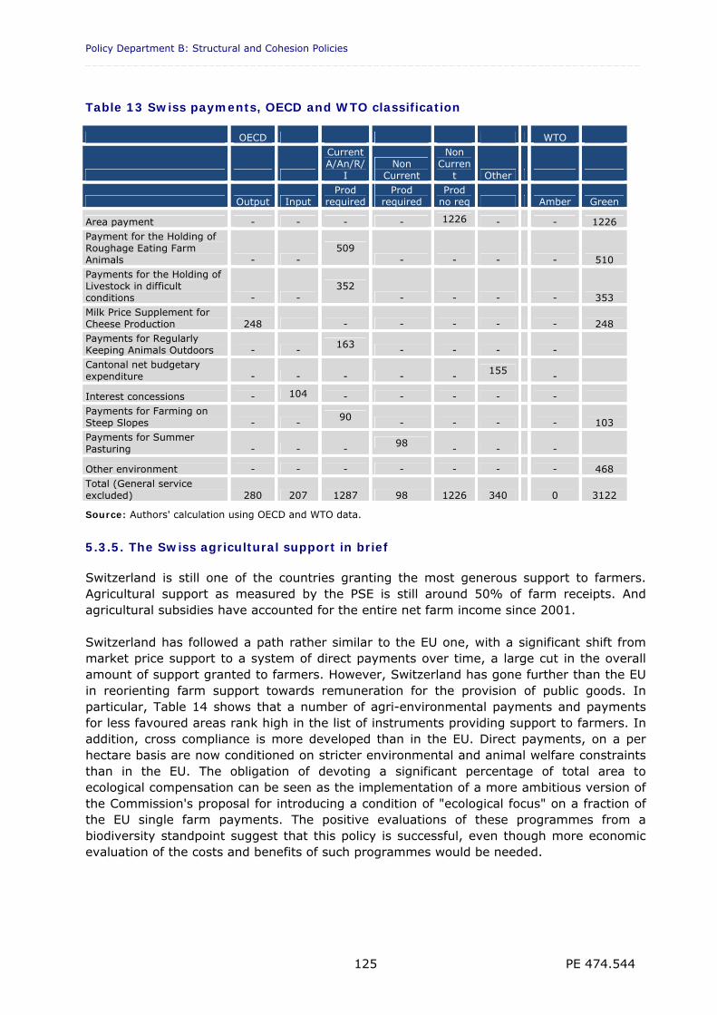
Policy Department B: Structural and Cohesion Policies _________________________________________________________________________________
PE 474.544 125
Table 13 Swiss payments, OECD and WTO classification
OECD WTO
Current A/An/R/
I Non
Current
Non Curren
t Other
Output Input Prod
required Prod
required Prod
no req Amber Green
Area payment - - - - 1226 - - 1226 Payment for the Holding of Roughage Eating Farm Animals - -
509 - - - - 510
Payments for the Holding of Livestock in difficult conditions - -
352 - - - - 353
Milk Price Supplement for Cheese Production 248 - - - - - 248 Payments for Regularly Keeping Animals Outdoors - - 163 - - - - Cantonal net budgetary expenditure - - - - - 155 -
Interest concessions - 104 - - - - - Payments for Farming on Steep Slopes - - 90 - - - - 103 Payments for Summer Pasturing - - - 98 - - -
Other environment - - - - - - - 468 Total (General service excluded) 280 207 1287 98 1226 340 0 3122
Source: Authors' calculation using OECD and WTO data.
5.3.5. The Swiss agricultural support in brief
Switzerland is still one of the countries granting the most generous support to farmers. Agricultural support as measured by the PSE is still around 50% of farm receipts. And agricultural subsidies have accounted for the entire net farm income since 2001. Switzerland has followed a path rather similar to the EU one, with a significant shift from market price support to a system of direct payments over time, a large cut in the overall amount of support granted to farmers. However, Switzerland has gone further than the EU in reorienting farm support towards remuneration for the provision of public goods. In particular, Table 14 shows that a number of agri-environmental payments and payments for less favoured areas rank high in the list of instruments providing support to farmers. In addition, cross compliance is more developed than in the EU. Direct payments, on a per hectare basis are now conditioned on stricter environmental and animal welfare constraints than in the EU. The obligation of devoting a significant percentage of total area to ecological compensation can be seen as the implementation of a more ambitious version of the Commission's proposal for introducing a condition of "ecological focus" on a fraction of the EU single farm payments. The positive evaluations of these programmes from a biodiversity standpoint suggest that this policy is successful, even though more economic evaluation of the costs and benefits of such programmes would be needed.
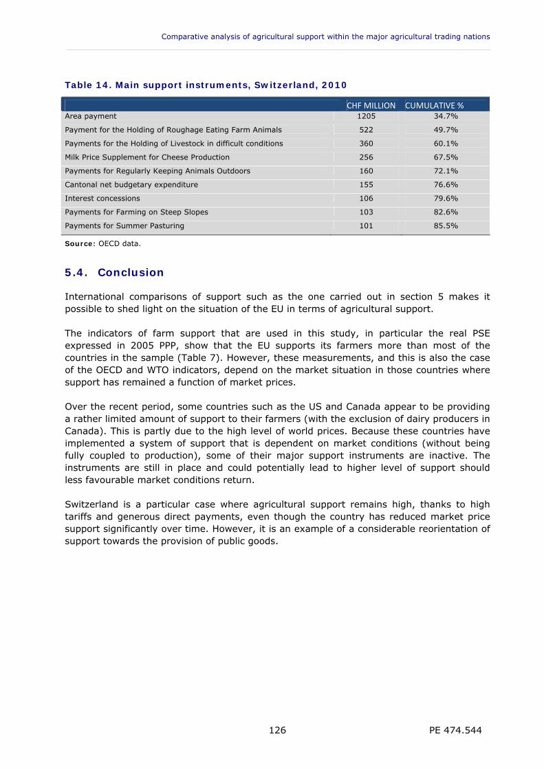
Comparative analysis of agricultural support within the major agricultural trading nations ___________________________________________________________________________________________
PE 474.544 126
Table 14. Main support instruments, Switzerland, 2010
CHF MILLION CUMULATIVE % Area payment 1205 34.7%
Payment for the Holding of Roughage Eating Farm Animals 522 49.7%
Payments for the Holding of Livestock in difficult conditions 360 60.1%
Milk Price Supplement for Cheese Production 256 67.5%
Payments for Regularly Keeping Animals Outdoors 160 72.1%
Cantonal net budgetary expenditure 155 76.6%
Interest concessions 106 79.6%
Payments for Farming on Steep Slopes 103 82.6%
Payments for Summer Pasturing 101 85.5%
Source: OECD data.
5.4. Conclusion
International comparisons of support such as the one carried out in section 5 makes it possible to shed light on the situation of the EU in terms of agricultural support. The indicators of farm support that are used in this study, in particular the real PSE expressed in 2005 PPP, show that the EU supports its farmers more than most of the countries in the sample (Table 7). However, these measurements, and this is also the case of the OECD and WTO indicators, depend on the market situation in those countries where support has remained a function of market prices. Over the recent period, some countries such as the US and Canada appear to be providing a rather limited amount of support to their farmers (with the exclusion of dairy producers in Canada). This is partly due to the high level of world prices. Because these countries have implemented a system of support that is dependent on market conditions (without being fully coupled to production), some of their major support instruments are inactive. The instruments are still in place and could potentially lead to higher level of support should less favourable market conditions return. Switzerland is a particular case where agricultural support remains high, thanks to high tariffs and generous direct payments, even though the country has reduced market price support significantly over time. However, it is an example of a considerable reorientation of support towards the provision of public goods.
Policy Department B: Structural and Cohesion Policies _________________________________________________________________________________
PE 474.544 127
6. EU SUPPORT IN THE FUTURE
KEY FINDINGS
The EU has largely shifted to production neutral instruments and provides fixed and more decoupled payments to farmers. The comparison of support with the other countries assists in exploring some of the issues discussed regarding the post 2013 CAP.
Compared to the EU, the US support focuses more on instruments that depend on market conditions and protect producers from market downturns. Canadian support focuses more on risk management. However, making EU payments more countercyclical would generate many unwanted and unproductive effects. And the poor transfer efficiency of US and Canadian insurance schemes calls for more investigation before further developing these instruments in the EU.
The success of the Swiss policy suggests that the "ecological focus" proposed by the Commission could have a positive impact on halting biodiversity erosion. However, the Swiss policy is more ambitious than the EU one in this area and the costs and benefits of such a similar policy in the EU should be assessed more thoroughly.
Agricultural support in emerging countries is growing rapidly and targets some strategic objectives. The development of support to research, innovation and infrastructure in Brazil contrasts with support in the EU that tends to mostly target farmers' income.
6.1. The future CAP
6.1.1. The Commission proposals
Since the 2008 declaration of the Presidency of the Council on the future of the Common Agricultural Policy, there has been an intensive debate about the definition of a CAP for the post 2013 period. The debates have been presented extensively in another publication of the European Parliament (see EP, 2010, section 2 in particular). After consultation with stakeholders, the Council and the Parliament, the Commission released two documents that can be used to assess what the future CAP might look like. The first one is the Commission’s proposal on the EU budget 2014-2020, released on June 29 2011. The second one is the legal proposal for the CAP, released on October 12 2011. The framework set out in the proposal for the Multiannual Financial Framework (MFF) proposal foresees that the CAP should maintain its two pillar structure with the budget for each pillar maintained in nominal terms at its 2013 level. Direct payments should promote sustainable production and 30% of their budgetary envelope should be devoted to measures that are beneficial to climate and the environment. Payment levels should progressively converge and payments to large beneficiaries should be subject to progressive capping. Rural development should be included in a Common Strategic Framework with other EU shared management funds with a reinforced outcome-orientated approach and subject to clearer, improved ex-ante conditions. The financing of the CAP should be reinforced with two instruments outside the MFF: 1) an emergency reserve to
Comparative analysis of agricultural support within the major agricultural trading nations ___________________________________________________________________________________________
PE 474.544 128
react to crisis situations and 2) the extension of the scope of the European Globalization Adjustment Fund. The Commission has proposed an adaptation of the CAP that aims to reduce some of the existing inefficiencies. The main elements of the Commission’s proposal from October 2011 regarding market measures and agricultural support are presented in Box 6.1. Relying on the European Parliament’s reports, The Commission drafted a legislative proposal attempting to reduce the inefficiencies as well as to address the questionable distribution issues of the current CAP. Should the proposal be adopted by the Council and the Parliament, the unequal distribution of the single farm payments would be reformed by shifting away from historical references, capping payments, and implementing a more even rate of payments between Member States. The Commission's proposal would narrow the definition of "active farmers". The proposed reform of the payments introduces several layers targeting particular functions like environmental effort (green payment) or rural vitality in less favoured areas (payment for areas with natural constraints). Market intervention would also be streamlined including the removal of the sugar quotas and a single common market organisation with more flexibility as well as a package of instruments to deal with economic crises in a particular sector. The strengthening of the producers' organisations is intended to give farmers a bargaining position more balanced with the largely oligopolistic downstream sector. The negative side of the past reforms, in particular the fact that farmers now face more price volatility, is addressed through risk management instruments (see Box 6.1).
6.1.2. Budget proposal and the level of support
If we consider the amounts foreseen in the MFF proposals of June 29 2011 and the CAP reform proposal of October 12 2011, direct aids and market related expenditure would increase from €45.6 billion in 2013 to €46.2 billion in 2020 in nominal terms, i.e., a decrease in real terms. Rural Development measures would basically remain unaffected at €14.6 billion in 2020. In addition, the budget for most deprived persons would reach €0.4 billion in 2020. The CAP would also benefit from payments from agricultural research and innovation, which would reach €0.8 billion (these amounts can be seen as fencing a share of the existing R&D budget) and €0.5 billion as part of the European Globalisation Fund available for agriculture in 2020. Compared to the expected 2013 expenditure, the Commission estimate is that the reform would lead to save some €1.2 billion in 2020. Altogether, the main consequences of the reform would be a minor increase in the payments for rural development purposes. Because of the capping of direct payments, some of the budget would indeed be recycled in pillar 2 (the estimated amount is €0.19 billion in the Commission's proposal). Market related expenditure would be reduced by €0.6 billion, but it is necessary to add support measures that might be required due to market disturbance or crises, which are covered by a reserve for agricultural crises.
6.1.3. How the EU AMS would be affected by the reform?
Market management and support. As far as the AMS is concerned, the proposal of the Commission would have limited impact. The Commission estimates suggest a reduction in market-related expenditure of roughly €0.4 billion a year.35 Given that a new flexible
35 Appendix of the document Brussels, 12.10.2011 COM(2011) 625 final, 2011/0280 (COD).
Policy Department B: Structural and Cohesion Policies _________________________________________________________________________________
PE 474.544 129
instrument to deal with crises would be implemented, it would imply expenditure that is likely to be distorting and part of the Amber Box. The amounts that might be spent on crises are obviously unknown at this stage, but the reserve should reach €3.5 billion. In the proposal, public intervention is to cover common wheat, barley, maize, paddy rice, beef and veal, butter and skimmed milk powder. The rules for wheat are unchanged. Barley, maize, paddy rice as well as beef and veal are subject to a tendering process only, which should not lead to the calculation of a "Market Price support" under the WTO "Product-Specific Aggregate Measurements of Support". The elimination of the quotas on domestic sugar production and exports after September 2015. Currently, in spite of the quota, sugar price support is counted in the Amber Box. In the most recent notifications, sugar accounts for €1.7 billion in AMS, due to the calculation of a market price support between the EU administered price (€323.5/tonne) and a reference price (€193.8/tonne).36 Should the guaranteed price be eliminated after 2015, this would automatically lead to a reduction in the corresponding AMS. Direct payments. One question is whether the set of payments included in the Commission proposal would affect the EU support as measured by the AMS. The redistribution of direct payments between Member States and farmers should not affect the classification of EU support under WTO as long as any effect on production level is avoided. Payments to young farmers granted by EU Member States are currently notified under the Green Box. The proposed scheme (Article 36 of the Commission's proposal)37 relies on entitlements that need to be activated, as is currently the case for the Single Farm Payment. One may consider that such payments satisfy the criteria for being exempted from AMS calculation. The scheme would involve a maximum of €0.9 billion annually if these payments are capped at 2% of the national Pillar 1 envelope. Payments in areas with natural constraints, albeit in Pillar 1, would rely on the same mechanisms as the current Single Farm Payment (i.e., activation of payment entitlements). One may also consider that these payments would be exempted from AMS calculation. Things are perhaps more complex for the basic payment (Article 18-28 of the October 12 2011 proposal) and the green component (Articles 29-33) of the proposed scheme. The Commission's impact assessment states that eligibility criteria could be designed such that these payments are eligible for the Green Box. The elements used to define an "active farmer" would need to respect WTO Green Box criteria. This means payments cannot imply an obligation to produce. However, Swinbank (2012) argues that the Commission’s greening proposals could be in danger of infringing on the Green Box requirement that no production is required to qualify for payment. Nor would the greening component appear to fit within the Green Box exemption for payments under environmental programmes. Swinbank also warns that if the green payment were reported as a decoupled income support payment, it might breach the conditions set out in the Agreement on Agriculture, due in particular to the obligation of crop rotation, which involves growing three crops.38
36 This figure corresponds to the EU notifications for the marketing year 2008/2009. G/AG/N/EEC/ 2 April 2012. 37 In this section, the Articles quoted refer to the October 2011 proposal, i.e., COM(2011)625 final,
2011/0280(COD), Brussels, 12.10.2011 document. 38 Paragraph 6 of Annex 2 of the Agreement on Agriculture addresses the conditions necessary for a payment to
qualify as decoupled income support. Of particular relevance is sub-paragraph (b): The amount of such
Comparative analysis of agricultural support within the major agricultural trading nations ___________________________________________________________________________________________
PE 474.544 130
Swinbank also questions the measures regarding permanent pasture that targets a specific type of land. He believes that there is a danger with the Commission’s proposals that the green payment would not be considered a Green Box payment. Swinbank also raises the possibility that, if the basic payment can only be claimed if the greening conditions are met, then it could put even the basic payment at risk as a Green Box measure. If greening involves one payment, not two (i.e., the basic and green components of the same payment), then the whole of the payment could be ineligible for the Green Box. One may argue that there are current provisions in Member States Good Agricultural and Environmental Conditions requirements that already condition the current Single Farm Payment on growing three crops, that the eligibility of such payments to the Green Box has not been challenged, and that permanent pasture is not necessarily used for production. More generally, it is hard to imagine that greening conditions imposed on the current direct payments make them more distorting. However, from a legalistic point of view, eligibility to the Green Box of close to 80% of the Pillar one payment would therefore be at risk. Coupled payments. The possibility for Member States to use part of their national ceiling for direct payments for coupled support in certain sectors in clearly defined cases has perhaps more impact on the EU Amber Box than what the Commission's impact assessment of the proposal suggests.39 Indeed, the proposal states that the resources may be used for any coupled support, granted in specific regions facing particular situations where specific types of farming or specific agricultural sectors are particularly important for economic, environmental and /or social reasons. This corresponds to an extension of the existing coupled aid schemes for cotton, sheep meat and beef to any "sensitive" sector. The amounts could be significant. In the proposal of October 12 2011, Member States would be allowed to use up to 5% of their national ceilings for this support (or 10% in case their level of coupled support in at least one of the years of the period 2010-2013 exceeded 5%). In duly justified cases, Member states would be allowed to use more than 10% of their national ceiling. Potentially, if all Member states used the maximum recoupling, a 5% ceiling would involve a €2.1 billion budget. In the Commission's proposal the 'voluntary coupled support' scheme would de facto replace coupled payments under Article 68 of Regulation 73/2009. That is, the overall impact on the AMS would be limited. However, the current Article 68 includes a ceiling that limits the possible budgetary outlays in a more stringent way than the scheme included in the October 12 2011 proposal.40 Indeed, the reference to 3.5% of the national ceiling in Article 69 of Regulation 73/2009 does not seem to be maintained in the proposal. However, Article 39 (4) of the proposal refers to the setting of a ceiling that is decided by the Commission on a yearly basis. In addition, because of the requirement to motivate the need for coupled support, and the approval procedure by the Commission (all of which refers to a rather complex set of criteria under Articles 39, 40, 41 of the proposal) the
payment in any given year shall not be related to, or based on, the type or volume of production (including livestock units) undertaken by the producer in any year after the base period.
39 The impact assessment remains rather vague regarding this issue. It states that "care should be exercised in rewarding specific types of production e.g., through a grassland premium, and certainly not production per se". (Document 20.10.2011 SEC(2011) 1153 final/2, page 72). However if payments intend to promote particular production, it is likely that their Green Box status might be challenged.
40 The 2003 regulation allowed Member States to earmark up to 10% of their respective national subsidy ceilings for “specific supports to farming” in their national territories. This principle was extended in articles 68 and 69 of Regulation 73/2009, which provided a wider range of objectives which can be used for granting specific support and eased the conditions attached. However, within the overall restriction of 10% of national ceilings, there are further limitations; i.e., that the coupled subsidies are limited collectively to 3.5% of the national ceiling [Article 69(4)]; and the support provided for economically vulnerable farming [under 68 (1) (b) of Regulation 73/2009] shall be limited to that required to maintain (i.e., not increase) existing production.
Policy Department B: Structural and Cohesion Policies _________________________________________________________________________________
PE 474.544 131
budgetary amounts should be more limited than the proposed 5% of the ceiling. At this stage, it is difficult to assess how much the coupled payment proposed by the Commission might lead to an increase in the EU AMS. Pillar 2 measures. The provisions regarding rural development in the Commission's proposal would not affect the eligibility of these programmes for the Green Box, as long as the eligibility criteria are not strengthened. Extra subsidies for rural development would mostly come from the capping of direct payments (also in the Green Box). New expenditure for food safety measures, agricultural research and innovation, and schemes for most deprived persons would be either matched by savings or would be transferred from existing budgets under other policies. Insurance. Another potential impact on the AMS is the introduction of a new income insurance scheme in Pillar 2 that might generate a form of support that, in the WTO, might be seen as coupled to production. Indeed, currently, most insurance subsidies are notified in the Amber Box and counted as non product specific AMS. Only a small fraction of them are counted in the Green Box. Given the opposition of some Member States to an EU-wide funded insurance scheme, the Commission has proposed that this instrument be part of Pillar 2. That is, cofinancing from Member States would be required. Overall, the combination of the measures is such that for every euro paid into the mutual fund by farmers, an additional €0.65 would be contributed from Pillar 2. The new tool would see 70% of farmers' losses reimbursed by a mutual fund if income drops by at least 30% below a three year average figure. The conditions set out in Articles 38-41 of the proposal on Rural Development41 suggest that the EU subsidies to insurances schemes might be eligible for the Green Box. 42 Conclusion. Given the current AMS ceilings, and the limited risk that any WTO member mounts a successful challenge of the green component of the Pillar 1 payments proposed by the Commission, the questionable Green Box compatibility of the proposed scheme is hardly a problem. The issue would only become relevant if a Doha Agreement was reached. However, the Commission's proposal could potentially change the applied level of the EU AMS.
BOX 6.1. THE FUTURE ORIENTATION OF THE CAP? The Commission's proposal for a Post 2013 CAP, released on October 12 2011 includes a significant reorientation of the direct payments, new instruments for managing markets, and more focus on environmental issues. The main provisions are the following. The proposal builds on the budget proposal for the multi annual financial framework. Overall, spending on Pillar 1 would total €312 billion for the 2014-2020 period, and an extra €101 billion would be allocated to Pillar 2. This funding would be complemented by extra budget coming from other programmes, in particular €5.1 billion for research and innovation; €2.5 billion for food safety; €2.8 billion for food support to deprived persons;
41 Brussels, 12.10.2011 COM(2011) 627 final 2011/0282 (COD) 42 The WTO rules allow disaster relief if: (i) there is a formal recognition by government authorities that a natural
or other event, including a disease outbreak, is a disaster; (ii) the event results in a production loss that exceeds 30% of the average of production in the preceding three-year period or a three-year average based on the preceding five-year period, excluding the highest and the lowest entry; (iii) the payments apply only in respect to losses of income, livestock, land or other production factors due to the natural disaster in question.
Comparative analysis of agricultural support within the major agricultural trading nations ___________________________________________________________________________________________
PE 474.544 132
€3.9 billion for the new reserve for crises in the agricultural sector; €2.8 billion in the European Globalization Adjustment Fund. Market management. The intervention would remain in place for wheat (limited to 3 million tonnes a year), butter (capped a 30 000 tonnes), and skimmed milk powder (capped at 109 000 tonne). A tendering process, rather than an automatic buy in would be in place for barley, maize, paddy rice, beef and veal. Private storage aid would cover sugar (after the end of the quotas, which would take place in 2015), olive oil, flax, beef, butter, skimmed milk powder, pig meat and sheep meat. The aid to dispose of a surplus of milk powder and casein would be abolished. The recognition of producers' organisations would be extended to all sectors. Public intervention, private storage and export returns would be funded from a €3.5 billion "crisis reserve" separate from the CAP and Multi Annual Financial Framework. Direct payments. A "Basic Payment" scheme would replace the current Single Farm Payment and the Simplified Area Payment Scheme. All EU member states would have to move towards a uniform payment per hectare at the regional level by 2019. National envelopes for direct payments would be adjusted so that those that receive less than 90% of the EU average payment per hectare will receive more, so that the gap will be reduced by one third by 2018. Direct payments in excess of €150 000 would be capped at progressive rates with an absolute ceiling of €300 000 (exclusive of the greening component). A simplified flat rate system would be introduced for small farms, which would be also exempted from greening requirements. A greening element would be introduced. Some 30% of direct payments would be conditional on three measures: crop diversification (arable farmers would have to cultivate at least 3 crops a year, none accounting for more than 70% of the surface and each at least for 5%); designation of 7% of land as an ecological focus area; maintenance of permanent pasture. The remaining payments (i.e., 70% of the envelope) would continue to be based on cross-compliance, but with simplified requirements. Two extra layers of payments would be allowed, one for areas with natural constraints (in addition to the Less Favoured Areas payments under Pillar 2), the other for young farmers, both of which would be subject to limitations (a maximum of 5% of national envelope and 2% of Pillar 1 national envelopes, respectively). New criteria would be introduced for receiving direct payments, specifically that the farmer must be "active", i.e., receiving at least 5% of beneficiary earnings from agriculture (exemption for small farmers). Rural development would be reformed significantly, with new priorities. At least 25% of pillar 2 envelopes would be devoted to climate change mitigation and adaptation and land management measures (including organic farming). A new insurance scheme would see 70% of farmers' losses reimbursed by a mutual insurance fund if income falls below a certain threshold. Pillar 2 would partially fund this mutual fund, in addition to farmers' contributions. The rates of financing of some Pillar 2 measures by the EU budget would also be revised upwards (LEADER projects, innovation and knowledge transfers, etc.).
6.2. Alternative directions for the post 2013 CAP
The October 12, 2011 Commission proposal has triggered several reactions from Member States as well as Members of the European Parliament. Drawing up a list of the various positions and criticisms is outside the scope of this report, but some of them relate to the differences between instruments aimed at supporting farmers used by the EU and those
Policy Department B: Structural and Cohesion Policies _________________________________________________________________________________
PE 474.544 133
used by other countries. For selected issues the comparison carried out in Section 5 could help discussion.
6.2.1. Making support more countercyclical?
The examination of both US and Canadian agricultural support shows that these countries have designed farm support instruments that protect farmers from adverse market as well as weather situations to a much larger extent than the EU. Indeed, while EU support now relies mainly on fixed and decoupled payments, these countries have implemented schemes under which payments are triggered in cases of poor harvest or low prices. The US, in particular, relies more than the EU on countercyclical measures. In the EU, several stakeholders criticized the Commission's proposal as failing to protect farmers in low price periods such as the year 2009. The idea of adjusting payments to market conditions, i.e., turning the Single Payment Scheme into a countercyclical payment scheme, has been recently backed by some farmers' organizations and cooperatives in particular (see EP, 2010 for a review of the stakeholders 'positions). They have openly quoted the US model as an example. Should the US policy be a source of inspiration for the EU? Adjusting the EU payments downwards when market conditions are good and upwards when farm incomes are low would help in smoothing farm income variations. It might also make the current system more acceptable to the public opinion (for example, grain producers enjoyed both very high prices and direct payments in 2008 or 2011). However, in spite of some attractive features, making SPS payments countercyclical would have many unwanted effects. First, it would raise some administrative problems regarding the EU budgetary procedure. A possibility would be to require that a multi annual budget be spent over some years with variations over time depending on market conditions, but the operational design of such a scheme is not a trivial task. If successful, one may wonder what added value is brought by the countercyclical management: farmers might just as well handle the adjustment themselves with the help of the banking sector if the total value of direct payments over a period of several years is known beforehand. Second, it would blur the signals of excess supply or excess demand to producers and thus potentially lead to market imbalances. At a time where market prices send producers the signal that stocks are low and demand is high, government intervention would introduce a rather inefficient dampening of such signals. Third, making the payments depend on the market situation would strongly limit the ability to condition payments on GAECs or other cross compliance provisions. Incentives from cross-compliance would be weakened in times of booming markets, when they are needed most. Conversely, cross-compliance incentives would be reinforced when low prices would also operate towards less intensive production methods. Would-be-providers of public goods need to have a predictable horizon, given the sunk costs that are often necessary to shift to different production techniques.43
43 In the case of payments that intend to favour the provision of public goods, one may even consider that
payments should be made procyclical rather than countercyclical in order to keep the provision of public goods attractive when market prices are high. Indeed, as farmers tend to decrease participation in agri-environmental schemes and voluntary set-asides when agricultural commodity prices are high, this should not be encouraged by reducing the environmental payments in these periods.
Comparative analysis of agricultural support within the major agricultural trading nations ___________________________________________________________________________________________
PE 474.544 134
Fourth, designing the income support component of the SPS as a substitute for market regulation would be difficult to manage given that the prices of all products do not vary evenly. It would basically require a return to product specific payments, which would be a radical turnaround for the CAP. Countercyclical payments would require, de facto, shifting back to product-specific payments. Finally there might be some inconsistencies with the EU multilateral commitments under the WTO framework. While such a scheme would be compatible with current multilateral commitments given the gap between current AMS and the AMS ceiling, the future limits on distorting support might be constraining in case of a Doha agreement. The Commission has not proposed turning the EU Single Farm Payment into an instrument that adjusts to market conditions as is the case with several US and Canadian schemes. Overall, the risk is that EU producers remain more exposed to variations in market conditions than US and Canadian ones. However, because of the economic inefficiency and the distortions involved in the US schemes, the US policy hardly appears as an example that should be followed. Making EU payments countercyclical would involve a de facto recoupling of the payments to particular products. For the EU to adopt schemes which required supplementary budgetary allocations of several billion Euro (as typical for the US), the EU budget would need to be much more flexible.
6.2.2. More risk management tools, including insurance schemes?
The US and Canada rely much more than the EU on insurance based support. In the US, public subsidies to insurance now represent a large share of the overall support to farmers (see Annex 5.1. and EP, 2009 for details on the US insurance schemes, ACRE and SURE). The Commission proposal is much less ambitious in terms of income insurance in particular. The risk management tools that are proposed by the Commission cover (i) crop, animal and plant insurance against economic losses caused by adverse climatic events and animal or plant diseases or pest infestation; (ii) mutual funds to pay financial compensations to farmers, for economic losses caused by the outbreak of an animal or plant disease or an environmental incident; (iii) an income stabilisation tool in the form of financial contributions to mutual funds, providing compensation to farmers who experience a severe drop in their income. The item (iii) is clearly an innovation, even though some similar schemes existed in some Member States. Should the EU move towards a US/Canadian approach? Government intervention has a role to play in insurance, at minimum by providing transparent information allowing for private companies to supply index based weather insurance, for example. In the case of catastrophes, epizooties and other particular hazards, the need for public funded insurance schemes or disaster compensation is hardly questioned. However, going further than the Commission's proposal towards an EU wide income stabilisation scheme would need to be more clearly documented. First, there is little European value added in insurance scheme management. Several Member States, not subsidizing their own insurance systems, have repeatedly expressed their reluctance over such a scheme during the Health Check debate. Second, an EU wide insurance scheme might lead to large interannual variations in expenditure, which would
Policy Department B: Structural and Cohesion Policies _________________________________________________________________________________
PE 474.544 135
require more flexibility in the EU budget.44 Third, evaluations of the US insurance scheme stress the cost for the public budget and the low efficiency in transfers when one compares the cost paid by the taxpayer and the government to the payments received by farmers (Glauber, 2007; Babcock and Hart 2006; Gardner 2008, Babcock 2009). Management costs, in addition to possible rents and leakages are associated with insurance schemes. From a transfer efficiency standpoint, it is unlikely that farmers would be better off with a given budget spent for subsidizing insurance rather than a direct payment, at a constant budget (under reasonable assumptions on the farmers' expected utility function). Rather than implementing an ambitious US type system of insurance and disaster payments, the Commission designed instruments (through the reserve for crises) that find some inspiration in the package of measures implemented by the Commission to cope with the dairy crisis in 2009. Consequently, EU producers remain more exposed to adverse conditions than do those in the US. However, the system of direct payments proposed by the Commission remains a more efficient way to transfer money to farmers than the costly US insurance scheme.
6.2.3. More ecological compensation areas?
The Swiss farm support policy targets the provision of public goods much more than does the policy of the EU especially with respect to landscape, water management, rural vitality, and biodiversity. The degree of reorientation of the CAP budget towards the funding of such public goods has been the subject of intense debate during the elaboration of the CAP reform proposal (see EP, 2010 for the positions of the different stakeholders, and TWG3, 2011 for proposals regarding public goods). In practice, the October 12, 2011 Commission proposal has not focused as much on the provision of such public goods as environmental organisations expected.45 The plan to "green" CAP support by making a fraction of the payments conditional on environmental practices is perhaps the issue that has raised the most criticisms after the Commission unveiled its CAP plans for post 2013. Agricultural organisations such as the COPA-COGECA, as well as some Member States and some Members of the European Parliament criticized the "ecological focus" as being de facto a "7% set-aside".46 They claim that it would be illogical to leave land idle at times of growing world demand. At the same time, the Commission's plan has been criticized for having "weak, vague conditions" (Greenpeace), while the WWF suggested that 100% of the subsidies rather than 30% should be subject to greening requirements. Should the EU copy the Swiss policy? Switzerland has developed an ambitious policy to protect biodiversity and water, which relies in particular on cross compliance for direct
44 The potential magnitude of the US payments under the insurance, ACRE and SURE programs is very large.
Orden et al. (2008) concluded that if the 1980s structure of prices were to reoccur, ACRE payments would reach very high levels for a few years. They find it difficult to predict whether such payments will fit in a particular year. The expected amount could be included in a range of USD 1 to 17 billion (see Zulauf 2008).
45 On October 2011, environmental NGOs expressed their disappointment at the Commission's proposal accusing the Commission of watering down the plans to promote public goods so much that they amounted to "greenwashing". See the position of BirdLife Europe, Friends of the Earth Europe, WWF (Agra Europe, October 18, 2011, p. 7).
46 Note that this claim is partly unfounded since the ecological focus area is not a compulsory set aside in the sense that all productive activity is forbidden. In addition, it is estimated that the current situation, where farmers cannot use some section of their fields (where there are hedges and borders in addition to the buffer strips) corresponds on average to 3% to 4% of the agricultural area, meaning that the additional effort is closer to 3%.
Comparative analysis of agricultural support within the major agricultural trading nations ___________________________________________________________________________________________
PE 474.544 136
payments. In this area, the Swiss experience goes beyond what the Commission proposes for the post 2013 CAP. Ecological compensation was initiated under the agri-environmental schemes in the 1990s and has become part of the conditions for eligibility for direct payments in 1998. Switzerland is the first European country where cross compliance was used directly for the promotion of biodiversity, even though in the 1990s and 2000s, the EU also conditioned direct payments on set-aside land, which had some ecological interest (at the time requirements allowed for the set-aside to be rotational, i.e., with more limited benefits for flora and fauna than the Swiss schemes). In Switzerland, in order to receive direct payments, farmers must manage at least 7% of their land as an ecological compensation surface. It is estimated that roughly 88% of farmers, accounting for 97% of total agricultural area in Switzerland meet these conditions. If one accounts for other environmental programmes that complement the requirement of ecological compensation for obtaining the direct payments, surfaces devoted to such an ecological use account for 13.6% of Swiss agricultural area according to Trometter et al. (2008). Environmental assessments of the different agri-environmental programs conclude that generally positive effects occur, but the magnitude of these effects differs. Lebeau and Righetti (2008) conclude that the positive effects on the quality of biodiversity have been rather modest. Aviron et al. (2009) monitored the effectiveness of cross compliance in promoting biodiversity on grassland and on arable land over an eight-year period in Switzerland. They observed measurable benefits for flora, butterflies, ground beetles, and spiders, in terms of species numbers and/or community composition, but little benefit for some threatened species. Some other estimates rank Switzerland highest in terms of the effectiveness of agri-environmental policies to preserve biodiversity. While in most cases the impact of the Agri-Environmental Schemes in the EU is either uncertain or disappointing, in Switzerland results appear more convincing (Herzog and Walter 2005; Albrecht et al. 2007). According to Trometter et al. (2008) Switzerland appears as the only European country where agri-environmental measures involve a significant positive impact on biodiversity erosion. Such erosion is dramatic and has accelerated over time in the EU.47 (see BirdLife 2011; Jiguet 2011). The scientific assessments are perhaps not consistent enough to conclude that the ecological compensation surface explains the better performance of the Swiss conservation policy compared to the EU schemes. Should further scientific results reach this same conclusion, then this should be a source of inspiration for the EU. Indeed, the Commission’s proposal of conditioning 30% of the direct payments on a series of constraints including an "ecological focus area" would draw the CAP closer to the Swiss policy. Introducing some ecological conservation areas would also rebalance the EU environmental policy towards a "land sparing" option, while the EU rural development has traditionally relied on "land sharing", i.e., putting the farm system at the core of the provision of
47 The Pan-European Common Bird Monitoring Scheme has compiled population figures for 145 common and
widespread bird species in 25 European countries between 1980 and 2009. Among those species covered, farmland birds are the most threatened group, with 20 out of 36 species in decline, and overall numbers at an all-time low, down by 48% since 1980. Some of the species that have declined the most over the last three decades include familiar farmland birds like Grey Partridge Perdix perdix (–82%), Skylark Alauda arvensis (–46%), Linnet Carduelis cannabina (–62%) and Corn Bunting Miliaria calandra (–66%). Figures from national inventories, in particular the STOC data in France, show very large decreases too, including for skylark with a decline of 71% over the last 20 years.
Policy Department B: Structural and Cohesion Policies _________________________________________________________________________________
PE 474.544 137
ecosystem services. Recent findings in ecology suggest that the land sparing option is an option that deserves consideration in the EU. The current proposal for an ecological focus involves economic costs. Its ability to make a significant difference in the dramatic erosion of biodiversity deserves more scientific assessments, in particular regarding the linkages of the conservation areas and the existence of threshold effects.
6.2.4. More emphasis on research and innovation?
The growth in agricultural output for selected emerging countries has been much higher than in the EU over the last decade. Brazil, in particular, had a growth rate of production exceeding 5% per year since 1995. One explanation is the priority that Brazil, as well as other leading emerging countries, has given to agricultural research and innovation as well as infrastructure. According to OECD figures, Brazil's public expenditure on agricultural research and development has tripled between 2007 and 2010, from 7% of General Services Support Estimates to 17%, i.e., USD 0.4 billion in 2010. The Agricultural Science and Technology Indicators, while giving much larger figures, confirm that public agricultural R&D spending has increased substantially in recent years due to the renewed commitment on the part of the Brazilian government.48 In spite of the uncertainty on the actual figures, both sources converge to indicate that Brazil and China have taken agricultural research and innovation as a priority in its farm support policy (Beinteima et al. 2010a, b). Research and innovation have never been formally part of the CAP. However, the Commission's proposal for the post 2013 CAP stresses the need for a major increase in research and innovation to address the urgent social challenges of providing more food in an environment of increasing land use competition and pressures on resources and the environment. Given the recent trends in EU yields whose growth has been declining for crops such as wheat, the question is whether the post 2013 CAP does enough to promote innovation (Chavas, 2011). Three instruments are envisaged in the Commission’s CAP reform proposals to support this agenda: (i) Continued support in the Rural Development Pillar 2 for investment in physical assets, business development, cooperation for the development of new products, processes and technologies in the agriculture and food sector as well as a revamping of farmer advisory services to broaden their scope and improve their effectiveness. (ii) A new European Innovation Partnership (EIP) instrument for agricultural productivity and sustainability also in the Rural Development Pillar; (iii) Increased funding for agricultural and food research under the Commission’s Horizon 2020 research programme (Matthews, 2012). The main role of the future EIP ‘Agricultural Productivity and Sustainability’ would be to look at the whole innovation cycle from R&D all the way to products or services on the market and enhance the effectiveness and the integration of innovation instruments. Actions would include cooperation, pilot-projects, knowledge transfer, advisory services, and dissemination. The objective is to put together a functioning network filling the current gap between farmers, rural enterprises, and advisors, on the one hand, and science on the other to allow the sector to take full advantage of innovation.
48 Brazilian Agricultural Research Corporation (Embrapa)’s 2009 spending, for example, was 28% higher than its
2008 spending (adjusted for inflation), its highest level, since inauguration. It is noteworthy that the progression of public agricultural R&D expenditure in China is even more impressive according to Beintema and Stads (2010a,b).
Comparative analysis of agricultural support within the major agricultural trading nations ___________________________________________________________________________________________
PE 474.544 138
In the Commission’s proposal on the multi-annual financial framework for 2014-2020, funding for the next EU research programme increases from less than €2 billion to €5.1 billion. It is instructive to realise that the sum of all national and EU outlays for research in agriculture and related biology, our upper bound estimate, is €4.2 billion per year for EU public R&D funding (2008 figures).49 This can be compared with the €43 billion provided as direct payments to EU farmers in 2008, or the €90.3 billion of transfers to farmers as measured as the OECD PSE. Even if the €5.1 billion EIP is approved, it will only be a small share of the €387 billion proposed total CAP budget. The Commission’s proposal suggests that the EU increase its budget on public agricultural R&D. However, the shift of EU expenditure away from farm income support to agricultural innovation is limited. One may question the persistent priority given to supporting farmers’ income rather than investing in the future, as do IPC (2011).
49 On an annual basis, IPC (2011) estimates that funding for Food, Agriculture and Technology under the
“Cooperation” item accounts for less than €300 million, out of the total R&D budget of roughly €8 billion per year. If one includes other programs such as capacity building, mobility of researchers, technology platforms, and total Community support, agricultural R&D efforts may reach €500 million. Member states also provide outlays on agricultural R&D, amounting to €3.7 billion in 2008.
Policy Department B: Structural and Cohesion Policies _________________________________________________________________________________
PE 474.544 139
7. CONCLUSION
Past reforms have made EU farm support more efficient in the sense that more of the transfers from taxpayers and consumers now reach the farmers' pockets. Leakages were larger with former policies such as price supports and export subsidies. The EU support now generates much less distortion in world markets. The EU also has a large degree of freedom regarding its international commitments, which focus on coupled and trade distorting forms of support. Regarding the levels of support, the PSE relative to production shows that the EU is among the average of OECD countries, at levels close to Russia, China and Canada. It is still double the level of support in the US on the basis of the percentage PSE. In many other OECD countries, the evolution of farm support has followed a rather similar path to that in the EU. Switzerland went further in shifting support towards the provision of public goods. Compared to the EU, the US and to some extent Canada, have maintained instruments that protect producers from market fluctuations. The US support is lower than the EU one, but part of the difference is explained by the current high level of world prices. Indeed, the US support relies more on countercyclical instruments than the EU. These instruments are not dismantled, they are simply inactive. This is an important difference from the EU support which relies on decoupled payments, more similar to lump sum transfers. Agricultural support in emerging countries has not evolved in the same way as in developed countries. In Russia and China, there has been strong growth in real support (in particular in China). Both countries support their agriculture in proportions that are similar to that in the EU, and higher if one accounts for the public support to general services. In addition, agricultural policies rely primarily on coupled support in these countries. While most OECD countries, and in particular the EU, have played by the rules regarding the WTO discipline, it is possible that in some emerging countries, which lag behind in their reporting, the level of distorting support measured by the AMS is now beyond their international commitments, but delays in the notifications do not allow for this conclusion, definitively. Finally, the analysis of general services shows that emerging countries such as Brazil and China invest heavily in research. The progression of the R&D expenditure in these countries dwarfs the efforts of the EU to increase public research budgets. As noted by several observers, the EU and US policies seem to keep focusing more on supporting farmers' income than investing in innovation.

Comparative analysis of agricultural support within the major agricultural trading nations ___________________________________________________________________________________________
PE 474.544 140
Policy Department B: Structural and Cohesion Policies _________________________________________________________________________________
PE 474.544 141
BIBLIOGRAPHY
Albrecht M., Duelli P., Muller C., Kleijn D., Schmid B. (2007). The Swiss agri-environment scheme enhances pollinator diversity and plant reproductive success in nearby intensively managed farmland. Journal of Applied Ecology 44(4): 813-822.
Anderson J. and Neary P. (1996). "A New Approach to Evaluating Trade Policy," Review of Economic Studies, vol. 63(1), pages 107-25, January.
Anderson J. and Neary P. (2003). "The Mercantilist Index of Trade Policy," International Economic Review, vol. 44(2), pages 627-649, 05.
Anderson J., Bannister G. and Neary P. (1995) Domestic Distortions and International Trade, International Economic Review, vol. 36(1), pages 139-57, February
Anderson J.E (1998). The Uruguay Round and welfare in some distorted agricultural economies, Journal of Development Economics, vol. 56(2), pages 393-410, August.
Antón J., Kimura S. and Martini R. (2011), “Risk Management in Agriculture in Canada, OECD Food, Agriculture and Fisheries Working Papers, No. 40, OECD, 94 p.
Atkinson A.B. (1970). On the Measurement of Economic Inequality, Journal of Economic Theory, 2, 244-263.
Aviron S., Nitsch H., Jeanneret P., Buholzer S., Luka H., Pfiffner L., Pozzi S., Schüpbach B., Walter T., Herzog F. (2009). Ecological cross compliance promotes farmland biodiversity in Switzerland. Frontiers in Ecology and the Environment 6: DOI: 10.1890/070197.
Babcock B. A. (2009). Prospects for ACRE payments in 2009. Iowa Ag Review, Winter 2009, 15, 1, 1-3.
Babcock B., A. and Hart C. (2006). Crop Insurance: A Good Deal for Taxpayers? Iowa Ag Review, Summer 2006, Vol. 12 No. 3.
Bakhshi S., Gray (2010) Is there Supply Distortion in Decoupled Payments? Evidence from the Canadian Prairies. Société canadienne d’agroéconomie, Denver 2010.
Balassa B. (1965). Tariff Protection in Industrial Countries: An Evaluation, Journal of Political Economy, Vol. 73, No 6, pp. 159-66.
Balassa B. (1971). The Structure of Protection in Developing Countries. Johns Hopkins University Press.
Baldwin R.E. and Robert-Nicoud F. (2007). Entry and Asymmetric Lobbying: Why Governments Pick Losers, Journal of the European Economic Association, MIT Press, vol. 5(5), pages 1064-1093, 09.
Balk B. M. (1995). Axiomatic Price Index Theory: A Survey. International Statistical Review 63, 69-93.
Ball V.E., Barkaoui A., Bureau J.C., Butault J.P. (1997). Aggregation Methods for Intercountry Comparisons of Prices and Real Values in Agriculture: A Review and Synthesis. European Review of Agricultural Economics, vol 24, n° 2, pp 183 206.
Barjolle D (2010); La politique agricole suisse entre économie, écologie et société. Economie Rurale N° 315, pp 6-8.
Comparative analysis of agricultural support within the major agricultural trading nations ___________________________________________________________________________________________
PE 474.544 142
Batten G. (2007) How Much Does Membership of the European Union Cost Britain? The Bruges Group. http://www.brugesgroup.com.
Beintema N. Avila F. and Fachini C. (2010a). Brazil, New Developments in the Organization and Funding of Public Agricultural Research. Agricultural Science and Technology Indicators, Country Note October 2010.
Beintema N. M. and Stads G J. (2010b). Public agricultural R&D investments and capacities in developing countries: Recent evidence for 2000 and beyond. ASTI background note prepared for the Global Conference on Agricultural Research for Development (GCARD), Montpellier, March 27–30, 2010. Washington, D.C.: International Food Policy Research Institute.
BirdLife (2011). Farmland birds in Europe fall to lowest levels. BirdLife Community. http://www.birdlife.org/community/2011/08/farmland-birds-in-europe-fall-to-lowest-levels/, accessed March 2012.
Blandford D., Josling T. and Bureau J.C. (2011). Farm Policy in the EU and the US. The Status of Reforms and the Choices Ahead. International Food and Agricultural Trade Policy Council. IPC discussion paper, Septembre 2011, 46 p.
Bourguignon F. (1979) Decomposable Inequality Measures, Econometrica, vol. 47, p. 901-920.
Bourguignon F., Morisson C. (1985), Une analyse de la décomposition de l’inégalité des revenus individuels, Revue Économique, n° 4, pp. 741-777.
Brink L. (2011). The WTO Disciplines on Domestic Support. In WTO Disciplines on Agricultural Support, Seeking a Fair Basis for Trade, Orden D, Blandford D. and Josling T eds, Cambridge University Press.
Buckwell (1997) Towards a common agricultural and rural policy for Europe, European Economy, EU Commission, DG for Economic and finacial Affairs, reports and Studies n°5.
Bureau J. C. and Kalaitzandonakes N. (1995). Measuring Effective Protection as a Superlative Index Number. American Journal of Agricultural Economics 77: 279-90.
Bureau J.C., Butault J.P. (1992). Productivity Gaps, Price Advantages and Competitiveness in E.C. Agriculture. European Review of Agricultural Economics, n°19, pp 25 48.
Bureau J-C. (2008). La Politique Agricole Commune. Collection Repères, La Découverte, Paris.
Bureau J. C., Fulponi L. and Salvatici S. (2000). Comparing EU and US Trade Liberalisation under the Uruguay Round Agreement on Agriculture. European Review of Agricultural Economics 27: 1-22
Butault J.P (2004).Les soutiens à l’agriculture : Théorie, histoire, mesure. Les éditions de l’INRA. 2004. 309 p.
Butault J.P (2011). Evolution of agricultural support in real terms in OECD countries and emerging economies. OECD, Food, Agriculture and Fisheries, Working Paper n° 37, 56 p.
Butault J.P, Bureau J.C. (2006). WTO Constraints and the CAP: Domestic Support in EU 25 Agriculture. TRADEAG report, European Commission.
Policy Department B: Structural and Cohesion Policies _________________________________________________________________________________
PE 474.544 143
Butault J.P. and Réquillart V. (2011). La stagnation de la production, l’essoufflement des gains de productivité et le déclin de la compétitivité de l’agro-alimentaire en France. INRA, Paris and Toulouse.
Butault J.P., Lerouvillois P. (1999). La réforme de la PAC et l’inégalité des revenus agricoles dans l’Union européenne. Economie et Statistique. N° 329-330, 1999-9/10.
Byerlee D., Morris M.-L. (1993). Calculating Levels of Protection: Is it always appropriate to use world reference prices based on current trading status? World Development, 21(5), p. 805-815.
Cahill C. and Legg W. (1989). Estimation of agricultural assistance using producer and consumer subsidy equivalents: Theory and Practice. OECD Economic Studies, No. 13, OECD, Paris.
Chavas J.P. (2011). Agricultural Policy in an Uncertain World. European Review of Agricultural Economiscs, 38, 3, August, 383-408.
Corden M. (1971). The Theory of Protection. Oxford, Clarendon Press.
Deaton A. and Heston A. (2009). Understanding PPPs and PPP-based national accounts, Working Papers 1186, Princeton University, Woodrow Wilson School of Public and International Affairs, Research Program in Development Studies.
Debar J-C. (2008). Un nouveau farm bill très protecteur. Agri US Analyse. Supplément n°5. Mai 2008, 3p.
Dewbre J. and Short C. (2002). Alternative Policy Instruments for Agricultural Support: Consequences for Trade, Farm Income and Competitiveness. Canadian Journal of Agricultural Economics, 50, 4, 443-464.
Dewbre J., Anton J., Thomson W. (2001). The transfer Efficiency and Trade Effects of Direct Payments. American Journal of Agricultural Economics, 83, 5, 120-1214.
Diakosavvas D. (2011). Evaluation des reformes de la politique agricole aux Etats-Unis. OCDE, 248 p.
Diakosavvas, D. (2002), “How to measure the level of agricultural support: Comparison of the methodologies applied by OECD and WTO” in Agricultural Policies in China after WTO Accession, OECD, Paris, pp. 217-245.
Diewert W. E. (1978).Superlative Index Numbers and Consistency in Aggregation. Econometrica, 46, 883-900.
Doyon M., Gouin D.-M., Paillat N. (2002). Analyse critique du concept d’ESP, estimation du soutien au producteur. Application au secteur laitier. Économie Rurale, n° 272, p. 74-87.
DTB Associates, LLP (2011), Domestic support and WTO obligations in key developing countries, septembre 2011, DTB Associates, LLP.
www.usarice.com/doclib/193/186/5652.pdf. Accessed March 2012.
Dworak T., Berglund M., Grandmougin B., Mattheiss V., Nyaggard Holen V. (2009). International review on payment schemes for wet buffer strips and other types of wet zones along privately owned land. Ecological institute, Berlin 40p.
EC (2009). Council Regulation (EC) 73/2009 of 19 January 2009 establishing common rules for direct support schemes for farmers under the common agricultural policy and establishing certain support schemes for farmers, amending Regulations (EC) No
Comparative analysis of agricultural support within the major agricultural trading nations ___________________________________________________________________________________________
PE 474.544 144
1290/2005, (EC) No 247/2006, (EC) No 378/2007 and repealing Regulation (EC) No 1782/2003, OJ L 30 , 31.1.2009, p. 16.
ECA (2011). Is agri-environment support well designed and managed? Special Report No. 7, European Court of Auditors, Luxembourg.
Effland A. (2011). Classifying and measurement agricultural support. Identifying differences between the WTO and OECD systems (2011). Economic Information Bulletin n° 74, USDA-ERS 24 p.
Eichhorn W. and J Voeller (1976). Theory of the Price Index. Lecture Notes in Economics and Mathematical Systems, Vol. 140, Berlin: Springer-Verlag.
EP (2007). Reflection on the possibilities for the future development of the CAP. Final Report, European Parliament. IP/B/AGRI/FWC/2006,- December. EuroCARE.
EP (2008).The U.S. Farm Bill 2008 and Comparison with the EU CAP After the Health Check. European Parliament. IP/B/AGRI/FWC/006-146. EuroCARE.
EP (2010). The Single Payment Scheme After 2013. New Approach-New Target. European Parliament. IP/B/AGRI/IC/2009-038. EuroCARE.
EP (2010b). The Implementation of The Health Check of the CAP in the Member States, in Particular With Regard to The New Articles 68 And 69 Of Regulation (Ec) N° 73/2009. Study IP/B/AGRI/IC/2009-074 May 2010 PE 431.604. E. Pitts, S. O’Grady, H. Wimmer.
ERS (1994). Estimates of Producer and Consumer Subsidy Equivalents: Government Intervention in Agriculture, 1982-92. U.S. Department of Agriculture, Economic Research Service. Washington, DC.
FAPRI (2001). Impacts of Additional Food Aid Allocations. FAPRI-UMC Report 15-01.
Féménia F., Gohin A. (2009). On the European responsibility in the agricultural multilateral trade negotiations: Modelling the impacts of the Common Agricultural Policy. World Economy, 32(10), pp. 1434-1460.
Gardner B. (2008). Does the Economic Situation of U.S. Agriculture Justify the Existing Commodity Programs? Available at: http://www.aei.org/research/farmbill/publications/pageID.1476,projectID.28/default.asp, accessed February 23 2009.
Glauber J.W. (2007). Double Indemnity: Crop Insurance and the Failure of U.S. Agricultural Disaster Policy. Working Paper prepared for "The 2007 Farm Bill & Beyond". American Enterprise Institute Agricultural Policy Series, Washington, DC.
Gohin A., Levert F. (2006). Comparer les politiques agricoles américaines et européennes : les indicateurs ESP sont-ils bien utiles ? Economie Rurale, n° 294-295, p. 92-106.
Guyomard H., Mahé L.-P.(1994). Measures of Distorting Support in the Context of Production Quotas. European Review of Agricultural Economics, vol. 21, p. 5-30
Haniotis T., Bascou p. (2003). The PSE: Is it reflecting or distorting, the trade impact of agricultural policies? Communication “Agricultural Policy Reform and the WTO: Where are we heading?”, Capri, 23-26 June 2003.
Harberger A. (1964). The measurement of waste. American Economic Review. May, 54:3, pp. 58-76.
Henry C. (1984). Microeconomics for Public Policy. Helping the Invisible Hand. Oxford University Press.
Policy Department B: Structural and Cohesion Policies _________________________________________________________________________________
PE 474.544 145
Hertel T. (1989b). PSEs and the Mix of Measures to Support Farm Incomes. World Economy, n° 12.1, p. 17-27.
Hines R. H. (1999). Three sides of Harberger Triangles. Journal of Economic Perspectives, Volume 13, Number 2—Spring 1999—Pages 167-188.
Howse R., Van Bork P. and Heberbrand C. (2006). WTO Disciplines and Biofuels: Opportunities and Constraints in the Creation of a Global Marketplace, International Food & Agricultural Trade Policy Council & Renewable Energy and International Law, October. 2006, 15-22.
ICTSD (2009). Agricultural Subsidies in the WTO Green Box. Ensuring Coherence with Sustainable Development Goals. Edited by: Ricardo Meléndez-Ortiz, Christophe Bellmann, Jonathan Hepburn, ICTSD, Geneva, Switzerland. Cambridge University Press.
IPC (2011). Keeping an Eye on the Ball: The Need to Prioritize US and EU Research and Development Funding for Agriculture. IPC Policy Brief, December. www.agritrade.org/Publications/FarmPolicyintheUSandEU.html.
Jiguet F. (2011). Suivi temporel des oiseaux communs : Résultats du programme STOC pour la France. http://www2.mnhn.fr/vigie-nature/spip.php?rubrique2 accessed March 2012.
Jones D. (2010). Analysing the Composition of Producer Support: New Tools and Methods. OECD, Paris.
Josling T. (1973). Agricultural Protection: Domestic Policy and International Trade. Supporting study, 9, Food and Agriculture Organisation, Rome.
Josling T. and Valdes A. (2004). Agricultural policy indicators. Fao Commodity And Trade Policy Research Working Paper, No. 4. Food and Agriculture Organisation, Rome.
Josling T., Blandford D. Earley J. (2010). Biofuel and Biomass Subsidies in the U.S., EU and Brazil:Towards a Transparent System of Notification. IPC Position Paper. September. International Food & Agricultural Trade Policy Council.
Josling T., Swinbank A. (2011). European Union. Chapter 3. In WTO Disciplines on Agricultural Support: Seeking a Fair Basis for Trade. Cambridge UK: Cambridge University Press. Orden D., Blandford D. and Josling T Eds.
Josling, T. (1973), Agricultural Protection: Domestic Policy and International Trade, c/73/LIM/9, FAO.
Josling, T. (1975), Agricultural Protection and Stabilisation Policies: a Framework of Measurement in the Context of Agricultural Adjustment, c/75/LIM/2, FAO.
Josling, T. and A. Valdés (2004), “Agricultural Policy Indicators”, FAO Commodity and Trade Policy Research Working Paper No. 4, FAO, Rome, www.fao.org/es/esa.
Josling, T. and S. Tangermann (1989), “Measuring Levels of Protection in Agriculture: A Survey of Approaches and Results”, in Alan Maunder and Alberto Valdés (eds), Agriculture and Governments in an Interdependent World: Proceedings of the Twentieth International Conference of Agricultural Economists.
Josling, Tim (2003). “Domestic Farm Policies and the WTO Negotiations on Domestic Support”, paper presented to the Conference on “Agricultural Policy Reform and the WTO: Where are we heading?” held at Capri (Italy), June 23-26.
Johnson R., Hanrahan C. and Schnepf R (2010). Comparing U.S. and EU Program Support for Farm Commodities and Conservation, CRS Report R40539.
Comparative analysis of agricultural support within the major agricultural trading nations ___________________________________________________________________________________________
PE 474.544 146
Kroll J.C., Barjolle D, Jouen M. (2010). Politiques agricoles et développement rural. Comparaisons entre la Suisse et la France. Economie Rurale N° 315, pp 9-24.
Krueger A., Schiff M. and Valdés A. (1988). Agricultural Incentives in Developing Countries: Measuring the Effect of Sectoral and Economywide Policies, World Bank Economic Review, Sept 1988, Vol. 2, No 3, September.
Legg W. (2002), The evolution of agricultural policies in OECD countries as reflected by the level and structure of support. In Agricultural Policies in China after WTO Accession, OECD, Paris, pp. 246-261.
Legg W. (2003). Agricultural Subsidies: Measurements and use in policy evaluation. Presidential address. Journal of Agricultural Economics, 54(2), p. 175-200.
Masters W.-A. (1993). Measuring Protection in Agriculture: the producer subsidy equivalent revisited. Oxford Agrarian Studies, 21(2), p. 133-142.
Matthews A. (2011). The mystery of the EU’s disappearing AMS. Capreform.eu. September 22nd. Available at: http://capreform.eu/the-mystery-of-the-eus-disappearing-ams/, accessed March 2012.
Matthews A. (2012). More on the European Innovation Partnership for Agricultural Productivity and Sustainability (EIP-A). Capreform.eu. January 19. Available at: http://capreform.eu/more-on-the-european-innovation-partnership-for-agricultural-productivity-and-sustainability-eip-a/, accessed March 2012.
McClatchy D. (1987). The Concept of Producer Subsidy Equivalent (PSE): Some Consideration with respect to International Negotiability. Agriculture Canada, Ottawa (May).
Mervoyer I., Beaumond H.-C., Kroll J.-C. (2001). Garanties et Soutiens publics aux Crédits à l’Exportation des Produits Agricoles aux États-Unis. Notes et Études Économiques, 14, p. 9-35.
Momagri (2011). Soutiens Globaux à la Production Agricole (SGPA) Présentation, résultats et enseignements pour les Etats-Unis et l’Europe, mimeo, Paris, 11 juillet.
O’ Donoghue E., Effland A., J. Cooper J., Chengxia Y (2011). Identifying overlap in the farm safety net. Economic Information Bulletin n° 87, USDA-ERS 38 p.
OCDE (2011a). Politique agricoles : Suivi et évaluation 2011. OECD, Paris.
OECD (1987). National Policies and Agricultural Trade. OECD, Paris.
OECD (2010). PSE Manual. Organisation for Economic Cooperation and Development. Unpublished. OECD, Paris.
OECD (2011b). Evaluation des réformes des politiques agricoles de l'Union Européenne. Editions OCDE, Paris.1
OECD (2011c). Disaggregated Impacts of CAP Reforms. Proceedings of an OECD Workshop. OECD, Paris.
Office Fédéral de l’Agriculture (2009). L’agriculture suisse en mouvement. La nouvelle loi sur l’agriculture. Un bilan dix ans après. Berne, 36 p.
Orden D., Blandford D., and Josling.T. (2008). Determinants of Farm Policies in the United States, 1996-2008. Presented at The 2008 Farm Bill in WTO Perspective Annual Meeting of the International Agricultural Trade Research Consortium, Scottsdale, AZ, December 7-9.
Policy Department B: Structural and Cohesion Policies _________________________________________________________________________________
PE 474.544 147
Orden D., Blandford D. and Josling T.(eds.) (2011). WTO Disciplines on Agricultural Support. Cambridge University Press.
Oskam A., Meester G. (2006). How useful is the PSE in determining agricultural support? Food policy, 31, p. 123-141.
Peters G.-H. (1989). The Interpretation and Use of Producer Subsidy Equivalents. Oxford Agrarian Studies, vol. 17, p. 186- 218.
Piketty T. (1997). L'économie des inégalités. La Découverte, Paris.
Portugal L. 2002. Methodology for the Measurement of Support and Use in Policy Evaluation. OECD, Paris.
Portugal, L. (2003). OECD work on defining and measuring subsides in agriculture, in Environmentally Harmful Subsidies: Policy Issues and Challenges, OECD, Paris.
Ritson C. and Harvey D. (1997). The Common Agricultural Policy, 2nd Edition . CAB International.
Rothertam L. (2008). Food For Thought. How the Common Agricultural Policy Costs Families £400 a Year. The Taxpayer Alliance, London.
Schnepf R and Hanrahan C. (2011). U.S. and EU Agricultural Support: Overview and Comparison. CRS Report R41713
Silberberg E. (1979). The Structure of Economics. Springer.
Skogstad G. (2011). Sommaire des buts de la politique gouvernementale canadienne de l’industrie agroalimentaire, ses objectifs et ses instruments. Contexte et perspectives sur les politiques agroalimentaires. Institut canadien des politiques alimentaires. Février 2011. 24 p.
Skogstad, G. (2008). Canadian Agricultural Programs and Paradigms: The Influence of International Trade Agreements and Domestic Factors. Canadian Journal of Agricultural Economics/Revue canadienne d'agroeconomie, 56(4), 493-507.
Sotte F. (2011). The CAP And The EU Budget. Do The Ex-Ante Data Tell The True? 122nd EAAE Seminar Evidence-Based Agricultural And Rural Policy Making: Methodological And Empirical Challenges Of Policy Evaluation Ancona, February 17-18, 2011.
Steenblik R. (2007). Biofuels – At What Cost? Government Support For Ethanol And Biodiesel In Selected Oecd Countries. Global Subsidies Initiative.
Sutton et al (2011a). The European Nitrogen Assessment. Sources, Effects and Policy Perspectives. Cambridge University Press, 664 p.
Sutton M.A., Oeenema O., Erisman J.W., Leip A., van Grinsven H., Winiwarter W. (2011b). Too much of a good thing. Nature 472, 159–161, 14 April 2011. doi:10.1038/472159a.
Swinnen J. (2010). Political Economy of Agricultural Distortions: The Literature to Date, Agricultural Distortions Working Paper 50308, World Bank.
Tangermann S. (2003). À propos du concept d’ESP: commentaires et réponse. Économie rurale, n°276, p. 69-72.
Tangermann S. (2005), “Is the Concept of the Producer Support Estimate in Need of Revision?”, OECD Food, Agriculture and Fisheries Working Papers, No.1, OECD, Paris, www.oecd.org/dataoecd/6/49/35091989.pdf.
Comparative analysis of agricultural support within the major agricultural trading nations ___________________________________________________________________________________________
PE 474.544 148
Tangermann S. (2006). Response to the article on “How useful is the PSE in determining agricultural support?” by Arie Oskam and Gerrit Meester. Food policy, 31, p. 142-147
Theil H. (1967), Economics and Information Theory, North-Holland Publishing Company, Amsterdam.
Thibodeau D., Clark J.S. (2009). Government Support, Transfer Efficiency, and Moral Hazard Within Heterogeneous Regions in Canadian Agriculture. IAAE.
Thompson (2011) S. Bénéfices et distribution des dépenses gouvernementales dans le secteur. Contexte et perspectives sur les politiques agroalimentaires. Institut canadien des politiques alimentaires. Février 2011. 12 p.
Trometter M., Deverre C., Doussan I., Fleury P., Herzog F., Lifran R. (2008). Chapitre 4. Biodiversité, agriculture et politiques publiques. Expertise collective INRA. Agriculture et biodiversité : rapport d'expertise pour les ministers de l'agriculture et de l'écologie. 634p. Accessible at http://www.inra.fr/l_institut/expertise/expertises_realisees/agriculture_et_biodiversite_rapport_d_expertisr (accessed March 2012).
TWG3 (2011). Public Goods And Public Intervention Synthesis Report (Final Version) March 2011. Thematic Working Group 3. European Network for Rural Development.
Tyers R. (1991). Implicit policy preferences and the assessment of negotiable trade policy reforms, European Economic Review, Elsevier, vol. 34(7), pages 1399-1426, November. 1990 issue.
USDA (1988). Estimates of Producer and Consumer Subsidy Equivalents: Government Intervention in Agriculture, 1982-86, ATAD, Economic Research Service, USDA, April.
Vernieres L. (1984). Equivalent Subvention à la Production. Une analyse critique. Direction de la Prévision. Ministère de l'Economie. Paris.
Westcott P., Price M. (2001). Analysis of the US commodity loan program with marketing loan provisions. USDA, Agricultural Economic Report 801, 26 p.
World Bank (2008), “Agriculture for Development”, World Bank Development Report 2008, World Bank, Washington D.C.
WTO (2000). Domestic Support: Background Paper by the Secretariat, Committee on Agriculture, G/AG/NG/S/1, 13 April.
Zulauf C. (2008). Selected Provisions Of Food, Conservation, And Energy Act Of 2008: Farm Income Support And Risk Management Programs. Ohio State University, May 2008
Policy Department B: Structural and Cohesion Policies _________________________________________________________________________________
PE 474.544 149
ANNEXES
Annex 1. The OECD indicators
Producer Support Estimate (PSE): the annual monetary value of gross transfers from consumers and taxpayers to agricultural producers, measured at the farm-gate level, arising from policy measures that support agriculture, regardless of their nature, objectives or impacts on farm production or income. Percentage PSE (%PSE): PSE as a share of gross farm receipts (including support). Producer Nominal Assistance Coefficient (producer NAC): the ratio between the value of gross farm receipts (including support) and gross farm receipts valued at border prices (measured at farm gate). Producer Nominal Protection Coefficient (producer NPC): the ratio between the average price received by producers at farm gate (including payments per tonne of current output), and the border price (measured at farm gate). Producer Single Commodity Transfers (producer SCT): the annual monetary value of gross transfers from consumers and taxpayers to agricultural producers, measured at the farm gate level, arising from policy measures directly linked to the production of a single commodity such that the producer must produce the designated commodity in order to receive the transfer. Producer Percentage Single Commodity Transfers (producer %SCT): the commodity SCT as a share of gross farm receipts for the specific commodity. Group Commodity Transfers (GCT): the annual monetary value of gross transfers from consumers and taxpayers to agricultural producers, measured at the farm gate level, arising from policy measures whose payments are made on the basis that one or more of a designated list of commodities is produced, i.e., a producer may produce from a set of allowable commodities and receive a transfer that does not vary with respect to this decision. All Commodity Transfers (ACT): the annual monetary value of gross transfers from consumers and taxpayers to agricultural producers, measured at the farm gate level, arising from policy measures that place no restrictions on the commodity produced but require the recipient to produce some commodity of their choice. Other Transfers to Producers (OTP): the annual monetary value of gross transfers from consumers and taxpayers to agricultural producers, measured at the farm gate level, arising from policy measures that do not require any commodity production at all. General Services Support Estimate (GSSE): the annual monetary value of gross transfers to general services provided to agricultural producers collectively (such as research, development, training, inspection, marketing and promotion), arising from policy measures that support agriculture regardless of their nature, objectives and impacts on farm production, income, or consumption. The GSSE does not include any transfers to individual producers. Percentage GSSE (%GSSE): GSSE as a share of Total Support Estimate (TSE). Consumer Support Estimate (CSE): the annual monetary value of gross transfers from (to) consumers of agricultural commodities, measured at the farm gate level, arising from policy measures that support agriculture, regardless of their nature, objectives or impacts on consumption of farm products. Percentage CSE (%CSE): CSE as a share of consumption expenditure (measured at farm gate) net of taxpayer transfers to consumers. Consumer Nominal Assistance Coefficient (consumer NAC): the ratio between the value of consumption expenditure on agricultural commodities (at farm gate) and that valued at border prices (measured at farm gate). Consumer Nominal Protection Coefficient (consumer NPC): the ratio between the average price paid by consumers (at farm gate) and the border price (measured at farm gate). Consumer Single Commodity Transfers (consumer SCT): the annual monetary value of gross transfers from (to) consumers of
Comparative analysis of agricultural support within the major agricultural trading nations ___________________________________________________________________________________________
PE 474.544 150
agricultural commodities, measured at the farm gate level, arising from policy measures directly linked to the production of a single commodity. Total Support Estimate (TSE): the annual monetary value of all gross transfers from taxpayers and consumers arising from policy measures that support agriculture, net of associated budgetary receipts, regardless of their objectives and impacts on farm production and income, or consumption of farm products. Percentage TSE (%TSE): TSE as a share of GDP
Policy Department B: Structural and Cohesion Policies _________________________________________________________________________________
PE 474.544 151
Annex 2. PSE categories and sub categories
A. Support based on commodity output A.1. Market price support (MPS) - transfers from consumers and taxpayers to agricultural producers arising from policy measures that create a gap between domestic market prices and border prices of a specific agricultural commodity, measured at the farm gate level. A.2. Payments based on output - transfers from taxpayers to agricultural producers from policy measures based on current output of a specific agricultural commodity. B. Payments based on input use: transfers from taxpayers to agricultural producers arising from policy measures based on on-farm use of inputs: B.1. Variable input use – transfers reducing the on-farm cost of a specific variable input or a mix of variable inputs. B.2. Fixed capital formation - transfers reducing the on-farm investment cost of farm buildings, equipment, plantations, irrigation, drainage and soil improvements. B.3. On-farm services - transfers reducing the cost of technical, accounting, commercial, sanitary and phyto-sanitary assistance, and training provided to individual farmers. C. Payments based on current A/An/R/I (1), production required: transfers from taxpayers to agricultural producers arising from policy measures based on current area, animal numbers, receipts or income, and requiring production. Category C is further Broken down to two sub-categories: C.1. Based on current receipts/income – including transfers through policy measures based on receipts or income. C.2. Based on current area/animal numbers – including transfers through policy measures based area/animal numbers. D. Payments based on non-current A/An/R/I, production required: transfers from taxpayers to agricultural producers arising from policy measures based on non-current (i.e., historical or fixed) area, animal numbers, receipts or income, with current production of any commodity required. E. Payments based on non-current A/An/R/I, production not required: transfers from taxpayers to agricultural producers arising from policy measures based on non-current (i.e., historical or fixed) area, animal numbers, receipts or income, with current production of any commodity not required but optional. Category E is further divided in two sub-categories according to the nature of payment rates used: E.1. Variable rates - transfers using payment rates which vary with respect to levels of current output or input prices, or production/yields and/or area. E.2. Fixed rates - transfers using payment rates which do not vary with respect to these parameters. F. Payments based on non-commodity criteria: transfers from taxpayers to agricultural producers arising from policy measures based on: F.1. Long-term resource retirement - transfers for the long-term retirement of factors of production from commodity production. The payments in this subcategory are distinguished from those requiring short-term resource retirement, which are based on commodity production criteria. F.2. A specific non-commodity output - transfers for the use of farm resources to produce specific non-commodity outputs of goods and services, which are not required by regulations. F.3. Other non-commodity criteria - transfers provided equally to all farmers, such as a flat-rate or lump-sum payment. G. Miscellaneous payments: transfers from taxpayers to farmers for which there is insufficient information to allocate them to the appropriate categories.
Comparative analysis of agricultural support within the major agricultural trading nations ___________________________________________________________________________________________
PE 474.544 152
(1). The abbreviations represent: A – Area; An – Animal numbers; R – Receipts; and I - Income Source: OCDE PSE Manual.
Policy Department B: Structural and Cohesion Policies _________________________________________________________________________________
PE 474.544 153
Annex 3. PSE labels
With or without current commodity production limits and/or limits to payments (with/without L): defines whether or not there is a specific limitation on current commodity production (output) associated with a policy providing transfers to agriculture and whether or not there are limits to payments in the form of limits to area or animal numbers eligible for those payments. Applied in categories A – F. With variable or fixed payment rates (with V/F rates): a payment is defined as subject to a variable rate where the formula determining the level of payment is triggered by a change in price, yield, net revenue or income or a change in production cost. Applied in categories A – E. With or without input constraints (with/without C): defines whether or not there are specific requirements concerning farming practices related to the programme in terms of the reduction, replacement, or withdrawal in the use of inputs or a restriction of farming practices allowed. Applied in categories A – F. – Payments conditional on compliance with basic requirements that are mandatory (with mandatory); – Payments requiring specific practices going beyond basic requirements and voluntary (with voluntary). Based on area, animal numbers, receipts or income (based on A/An/R/I): defines the specific attribute (i.e., area, animal numbers, receipts or income) on which the payment is based. Applied in categories C – E. Based on a single commodity, a group of commodities or all commodities (based on SC/GC/AC): defines whether the payment is granted for production of a single commodity, a group of commodities or all commodities. Applied in categories A – D. With or without commodity exceptions (with/without E): defines whether or not there are prohibitions upon the production of certain commodities as a condition of eligibility for payments based on non-current A/An/R/I of commodity(ies). Applied in Category E. Source: OCDE PSE Manual.

Comparative analysis of agricultural support within the major agricultural trading nations ___________________________________________________________________________________________
PE 474.544 154
Policy Department B: Structural and Cohesion Policies _________________________________________________________________________________
PE 474.544 155
Annex 4. The US layers of payments to farmers
Three US programs are designed to support farm incomes: direct payments, countercyclical payments and marketing loans. It relies on a complex system of several layers of payments. Marketing loan program. The "loan rates" are actually administratively set prices for each program crop, which guarantee that unit returns for farmers will be at least as high as the corresponding loan rate. Farmers then use the loans to finance their upcoming crops, with those crops used as collateral. If the market price for the crop is above the loan rate, the producer can repay the loan and keep the balance. If the market price falls below the loan rate, there are four options for farmers to obtain the loan rate rather than the lower market price as the effective producer price. First the government is obliged, at the farmer’s option, to receive the crops tendered as collateral into public stocks as full repayment for the loan (termed a "non recourse loan"). Second, the producer can choose to repay the loan at the ‘loan repayment’ rate. This loan repayment rate is usually set slightly below county level market prices such that producers will pay back the loan at the repayment rate and keep the difference between the market price and the loan repayment rate as an additional profit (termed ‘marketing loan gain’). A third option for farmers at any time after harvest, if market price is below the loan rate, is to either take out a ‘marketing loan’ from the government or simply to take a payment equal to the product of harvested production and the difference between the loan rate and the loan repayment rate. That is as if the farmer takes out a loan at the loan rate and then immediately pays back the loan at the loan repayment rate. This payment is called a loan deficiency payment (LDP). If the loan repayment rate equals the local cash price, and the farmer chooses to market the crop when the LDP is received, then the farmer effectively obtains the loan rate as a market price at harvest. The fourth option for producers to benefit from the marketing loan program is to buy marketing certificates from the USDA available at a price equal to the loan repayment rate. The quantity of certificates that the producer buys is equal to the quantity that the producer placed under loan. The producer can forfeit the loan to the government and buys back the amount placed under loan with the certificates. The marketing loan program allows USDA to guarantee that farmers receive at least the loan rate as a producer price for their crop without the need for government to actually take possession of crops. This means that market prices are free to adjust downward to clear domestic and international markets. "Direct payments". While there are other forms of direct payments (see below) this category includes transfers that are largely independent from price variations and to a large extent decoupled from production. The level of these payments is determined by multiplying a crop-specific direct payment rate by 85 percent of a farm’s direct payment base acres and payment yields (the 85 percent were changed temporarily to 83.3 percent under the FCEA, i.e., until 2011). Corn, wheat, soybeans, cotton and rice account for 95 percent of all direct payments. Countercyclical Payment Program (CCP). Payments under this program are triggered whenever the market price ("season-average" price) is less than the effective target price. Effective target prices are the difference between target prices and direct payment rates. The CCP payment rate equals the difference between the effective target price and the market price, but if market prices drop below loan rates, the latter are used to calculate payment rates. The amount of payment equals 85 percent of the product of the payment rate, a farm’s program yield, and a farm’s program acreage (the FCEA changes on the base
Comparative analysis of agricultural support within the major agricultural trading nations ___________________________________________________________________________________________
PE 474.544 156
acreage do not affect countercyclical payments). It is unclear to what extent these payments, which are linked to market prices but decoupled from current production, have impact on planting. Direct and countercyclical payments are made on the basis of each farmer’s base crop area and yield, irrespective of what is actually produced on the base area. For example, a farmer with a cotton base receives direct and countercyclical payments for cotton even if he or she is producing another crop, such as soybeans, or nothing at all. The only instances when program crop farmers are precluded from receiving any program payments are if they are producing fruit, vegetables or wild rice on their program bases. That does not mean that their impact on production is zero, given some indirect effects through risk reduction, alleviation of financial constraint, etc. However, it is quite limited. Because marketing loans guarantee farmers a minimum price for all production, they have the potential to influence acreage decisions more than any other program. Whereas direct payments and countercyclical payments may create some indirect incentives to change planting decisions, a guaranteed price creates a direct incentive. The ACRE program. A major change in the farm support with the 2008 agricultural Act is the introduction of an Average Crop Revenue Election (ACRE) program. Farmers may choose either to stay with the traditional CCP or this new revenue based ACRE option. The ACRE program is available for the same crops as traditional CCP payments, including pulses. Farmers must enter all of their eligible crops into the program, not just one or some. To receive an ACRE payment, two triggers need to be met. First, the actual state revenue for a supported crop must be less than the state level revenue guarantee amount. Second, the farm’s actual revenue for the same crop must be less than the farm’s benchmark revenue. The farm revenue trigger avoids the case where a farm would receive marketing loan and counter-cyclical payments even when it has above average revenue (due to high individual farm yields). The State revenue guarantee is computed as 90 percent of the product of an average guarantee yield and a price guarantee. The state guarantee yield is an Olympic average of the most recent five years. The price guarantee is the average over the most recent two years of the market price (or 70 percent of the marketing loan rate if higher). Changes in the State revenue guarantee are limited to plus or minus 10 percent from the previous year. As regards the farm benchmark revenue, it is also included as the product of a 5 year Olympic average crop yield and the ACRE price guarantee. Actual crop insurance premiums per acre paid by the farm are also included in this farm benchmark revenue (contrary to actual farm revenue) and thus provide an incentive to buy crop insurance. Whatever market conditions, participants in ACRE continue to receive direct payments, but with a 20 percent cut. Participants also continue to be eligible for marketing loan programs, but with a 30 percent lower loan rate. If both triggers mentioned above are met, the ACRE payment per acre will be provided, calculated as the difference between state revenue guarantee and actual state revenue or 25 percent of state revenue guarantee if lower. This per acre state payment is calculated at the farm level by applying a farm specific productivity ratio (given by a 5 year Olympic average farm crop yield per planted acre divided by the State guarantee yield). This farm level ACRE payment per acre is applied to 85 percent of farm planted acreage of the given crop. Thus ACRE payments are based on planted acres rather than base acres. However the total number of planted acres enrolled in ACRE cannot exceed the total number of base acres for all covered commodities on a
Policy Department B: Structural and Cohesion Policies _________________________________________________________________________________
PE 474.544 157
farm. If planted area exceeds base area farmers may enrol that crop mix ACRE that maximises total payments in the year of entering ACRE and beyond. The SURE program. The Supplemental Revenue Assistance program protects against crop losses resulting from adverse weather. While past disaster programs made payments based on individual crop losses and were often tied to base acres for either direct payments or countercyclical payments, SURE is a whole-farm disaster assistance program (all acres in all counties) that is tied to crop insurance coverage and farm planted. SURE covered the 2008–11 crop years. To qualify, a producer (a) must purchase insurance for insurable crops at a minimum coverage of 50 percent of yield and 55 percent of price and purchase Noninsured Crop Assistance Program (NAP) for non-insurable crops, and (b1) must farm in a county declared a disaster county or contiguous county, or (b2) has total farm production that is 50 percent or less of normal due to adverse weather. The farm-specific" program guarantee" is determined by a (complicated) formula. If SURE-computed actual revenue is below the farm specific SURE program guarantee and at least one of the two trigger events (county disaster or 50 percent farm revenue loss) has occurred, then SURE will pay out. The payments will be equal to 60 percent of the difference between the "program guarantee" and the "computed actual revenue", and capped at 90 percent of the "expected revenue".