Discontinuous Galerkin Methods on GraphicsProcessing Units for Nonlinear Hyperbolic

Conservation Laws

Martin Fuhry Lilia Krivodonova

June 5, 2013

Abstract

We present an implementation of the discontinuous Galerkin (DG) method forhyperbolic conservation laws in two dimensions on graphics processing units (GPUs)using NVIDIA’s Compute Unified Device Architecture (CUDA). Both flexible andhighly accurate, DG methods accommodate parallel architectures well, as theirdiscontinuous nature produces entirely element-local approximations. High perfor-mance scientific computing suits GPUs well, as these powerful, massively parallel,cost-effective devices have recently included support for double-precision floatingpoint numbers. Computed examples for Euler equations over unstructured trianglemeshes demonstrate the effectiveness of our implementation. Benchmarking ourmethod against a serial implementation reveals a speedup factor of over 50 timesusing double-precision with an NVIDIA GTX 580.

1 Introduction

Graphics processing units (GPUs) are becoming increasingly powerful, with some of thelatest consumer offerings boasting over a teraflop of double precision floating point com-puting power. Their theoretical computing performance compared with their price ex-ceeds that of nearly any other computer hardware. With the introduction of softwarearchitectures such as NVIDIA’s CUDA [13], GPUs are now regularly being used for gen-eral purpose computing. With support for double-precision floating point operations,they are now a serious tool for scientific computing. Even large-scale computational fluiddynamics (CFD) problems with several million element meshes can be easily handled ina reasonable amount of time, as video memory capacities continue to increase.

We describe an implementation of a modal discontinuous Galerkin (DG) method forsolutions of nonlinear, two-dimensional, hyperbolic conservation laws on unstructuredmeshes for GPUs. High-order DG methods can be particularly suitable for parallelizationon GPUs as the arithmetic intensity, that is, the ratio of computation time to memoryaccess time, for high-order methods is signifcantly higher than, e.g., finite difference andfinite volume methods due to the higher concentration of degrees-of-freedom per element.The amount of work per degree-of-freedom is also higher as it requires a computationallyintensive high-order quadrature rule evaluation over an element and its boundary.

1

Compared to structured grid methods, implementations of unstructured grid CFDsolvers have been sparse. Lower-order finite volume solvers handling nonlinear prob-lems in [1, 5] have been successfully applied. The most relevant example to this workis Kloeckner et al [10, 9], who implemented a high-order nodal DG method for linearhyperbolic equations. This approach simplifies computation by taking advantage of lin-earity, i.e., the integrals may be precomputed and the resulting structure is dominatedby a matrix-vector multiplication. Nonlinear solvers, on the other hand, must recom-pute nonlinear fluxes on each element and at every timestep. Thus, the main differencebetween linear and nonlinear DG solvers lies in the ability (or inability) to precomputethe majority of the work. In addition, Riemann solvers and, especially, limiters requirecareful incorporation into DG implementations for nonlinear problems.

In comparison to a serial implementation, we obtain a speedup of more than 50 timesusing double-precision with an NVIDIA GTX 580, which favorably compares with resultspresented in previous work [10, 9, 7, 1, 5, 8, 3]. At present, a meaningful comparisonbetween different implementations is difficult to make, as newer hardware rapidly replacesolder hardware. In addition, implementations performing in single-precision will currentlyoutperform those done in double-precision by a significant factor. At present, efficientimplementations achieve a 30-50 times speedup over comparable serial versions.

Our implementation demonstrates that a straightforward, but careful, approach canachieve a significant gain even for complicated problems. We see a comparable perfor-mance to [10] by operating on a much simpler thread-per-element and thread-per-edgebasis without needing to use shared memory between threads. As global memory trans-fers often represent the bottleneck for GPU computations, memory access patterns cancompletely determine the arithmetic intensity, and therefore, the overall performanceof the implementation. We diverge from the usual memory storage patterns by storingsolution coefficients, i.e. degrees of freedom associated with one element, appropriatelyallowing consecutive threads to access nearby data; in particular, we store these basis-function-wise as opposed to element-wise. We also extensively take advantage of constantmemory, storing all possible precomputed evaluations for fast access.

The two major components of our implementation involve evaluating an integral overan element and evaluating an integral over its boundary. While the former computation isstraightforward to implement, two different approaches may be taken towards implement-ing the latter. Element-wise integration over edges results in evaluating the same integraltwice. Edge-wise integration significantly increases thread count and avoids performingthis computation twice, but introduces race conditions for unpartitioned, unstructuredmeshes. Preventing these race conditions when parallelizing edge-wise proved particu-larly challenging, as atomic operators significantly degrade performance. Despite thesedifficulties, we found that the edge-wise approach provided roughly twice the performanceas the element-wise approach.

In the final section of our paper, we present several representative examples of theEuler equations with and without limiting. We measure runtime performance, speedupover a serial implementation, and scalability for order of approximation p ranging fromone to five. To take full advantage of the processing power available in our test GPUs,we found that a mesh size of roughly 10,000 elements suffices. With p = 1, we foundthat problems of up to four million elements can be easily handled for Euler equations.Finally, we found that while limiters certainly inhibit performance on GPUs as they do

2

on CPUs, performance in our implementation does not degrade significantly.

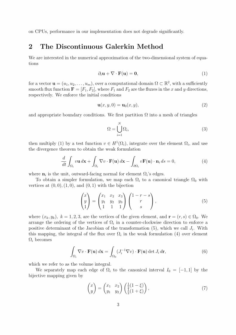
2 The Discontinuous Galerkin Method

We are interested in the numerical approximation of the two-dimensional system of equa-tions

∂tu +∇ · F(u) = 0, (1)

for a vector u = (u1, u2, . . . , um), over a computational domain Ω ⊂ R2, with a sufficientlysmooth flux function F = [F1, F2], where F1 and F2 are the fluxes in the x and y directions,respectively. We enforce the initial conditions

u(x, y, 0) = u0(x, y), (2)

and appropriate boundary conditions. We first partition Ω into a mesh of triangles

Ω =N⋃i=1

Ωi, (3)

then multiply (1) by a test function v ∈ H1(Ωi), integrate over the element Ωi, and usethe divergence theorem to obtain the weak formulation

d

dt

∫Ωi

vu dx +

∫Ωi

∇v · F(u) dx−∫∂Ωi

vF(u) · ni ds = 0, (4)

where ni is the unit, outward-facing normal for element Ωi’s edges.To obtain a simpler formulation, we map each Ωi to a canonical triangle Ω0 with

vertices at (0, 0), (1, 0), and (0, 1) with the bijectionxy1

=

x1 x2 x3

y1 y2 y3

1 1 1

1− r − srs

, (5)

where (xk, yk), k = 1, 2, 3, are the vertices of the given element, and r = (r, s) ∈ Ω0. Wearrange the ordering of the vertices of Ωi in a counter-clockwise direction to enforce apositive determinant of the Jacobian of the transformation (5), which we call Ji. Withthis mapping, the integral of the flux over Ωi in the weak formulation (4) over elementΩi becomes ∫

Ωi

∇v · F(u) dx =

∫Ω0

(J−1i ∇v) · F(u) det Ji dr, (6)

which we refer to as the volume integral.We separately map each edge of Ωi to the canonical interval I0 = [−1, 1] by the

bijective mapping given by (xy

)=

(x1 x2

y1 y2

)(12(1− ξ)

12(1 + ξ)

), (7)

3

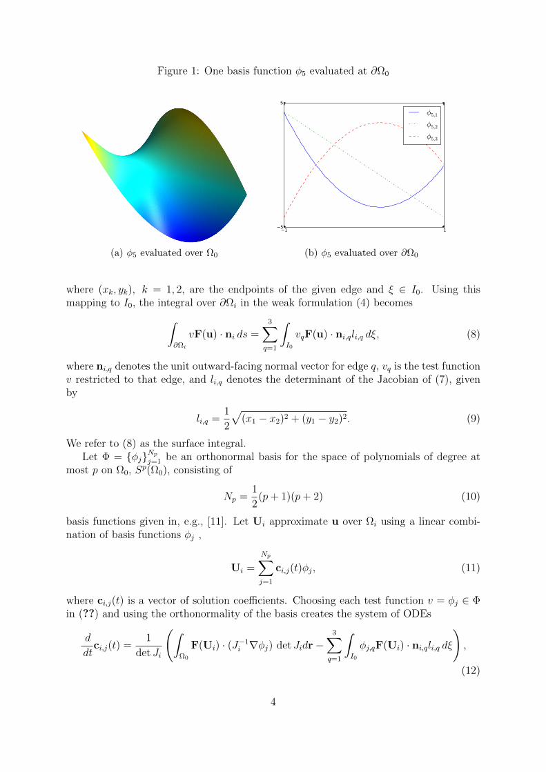
Figure 1: One basis function φ5 evaluated at ∂Ω0

(a) φ5 evaluated over Ω0

1 15

5

φ5,1

φ5,2

φ5,3

(b) φ5 evaluated over ∂Ω0

where (xk, yk), k = 1, 2, are the endpoints of the given edge and ξ ∈ I0. Using thismapping to I0, the integral over ∂Ωi in the weak formulation (4) becomes∫

∂Ωi

vF(u) · ni ds =3∑q=1

∫I0

vqF(u) · ni,qli,q dξ, (8)

where ni,q denotes the unit outward-facing normal vector for edge q, vq is the test functionv restricted to that edge, and li,q denotes the determinant of the Jacobian of (7), givenby

li,q =1

2

√(x1 − x2)2 + (y1 − y2)2. (9)

We refer to (8) as the surface integral.Let Φ = φjNp

j=1 be an orthonormal basis for the space of polynomials of degree atmost p on Ω0, Sp(Ω0), consisting of

Np =1

2(p+ 1)(p+ 2) (10)

basis functions given in, e.g., [11]. Let Ui approximate u over Ωi using a linear combi-nation of basis functions φj ,

Ui =

Np∑j=1

ci,j(t)φj, (11)

where ci,j(t) is a vector of solution coefficients. Choosing each test function v = φj ∈ Φin (??) and using the orthonormality of the basis creates the system of ODEs

d

dtci,j(t) =

1

det Ji

(∫Ω0

F(Ui) · (J−1i ∇φj) det Jidr−

3∑q=1

∫I0

φj,qF(Ui) · ni,qli,q dξ),

(12)

4

where φj,q denotes the basis function φj evaluated on the edge q, as demonstrated inFigure 1. Note that, in general, φj assumes different values on each edge q.

The numerical solution on the edges of each element is twice defined, as we do notimpose continuity between elements. To resolve these ambiguities, we replace the fluxF(Ui) on ∂Ωi with a numerical flux function Fn(Ui,Uk), using information from boththe solution Ui on Ωi and the solution Uk of the neighboring element Ωk sharing thatedge.

3 Implementation

GPU computing, while providing perhaps the most cost-effective performance to date, isnot without its challenges. The sheer floating point power dispensed by GPUs is onlyrealized when unrestricted by the GPUs limited memory bandwidth. As such, it is ofparamount importance to carefully manage memory access. The three main CUDA mem-ory containers we use in this implementation are the global, local, and constant memories.Global memory on the GPU is very large, but is very slow to access, introducing largelatencies. We therefore manage global memory by minimizing these memory accesses,coalescing the necessary global memory transactions by instructing nearby groups ofthreads to access the same blocks of memory. Local memory is physically located inglobal memory, but is cached, allowing much faster access. Constant memory is cachedand extremely fast, but very limited.

Programming GPUs using CUDA is unlike programming CPUs [13]. CUDA machinecode is separated into kernels - parallel code to be executed on the GPU. Global data indedicated video memory is manipulated by many threads running the same instructionset. Programming is done from a thread perspective, as each thread reads the sameinstruction set, using it to manipulate different data. Threads have a unique numericidentifier, a thread index, allowing, e.g., each thread to read from a different memorylocation. In order to take full advantage of the processing power available, enough warps,that is, collections of sixteen threads, must be created to fully saturate the device. Loadbalancing is done entirely by CUDA’s warp scheduler. When memory access requestsintroduce latency, e.g., global memory access requests, the warp scheduler will attemptto hide the latency by swapping out the idle warps and replacing them with ready warps.Problems with low arithmetic intensity spend most of their run time waiting duringlatencies in memory transactions. Problems with high arithmetic intensity, on the otherhand, allow CUDA’s warp scheduler to hide memory latency behind computation byscheduling ready warps ahead of those waiting on memory transactions.

Boolean expressions pose problems for GPUs, as two threads in the same warp mayevaluate a boolean condition to different values. When this happens, the warp splitsinto branches, where each branch of threads executes a different path of code split by theboolean. This branching, called warp divergence, harms performance as both instructionsmust be run for this warp.

Below, we give a brief overview of our parallelization approach for this implementation.The following subsections provide more detailed descriptions of our method. The right-

5

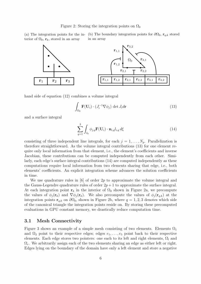
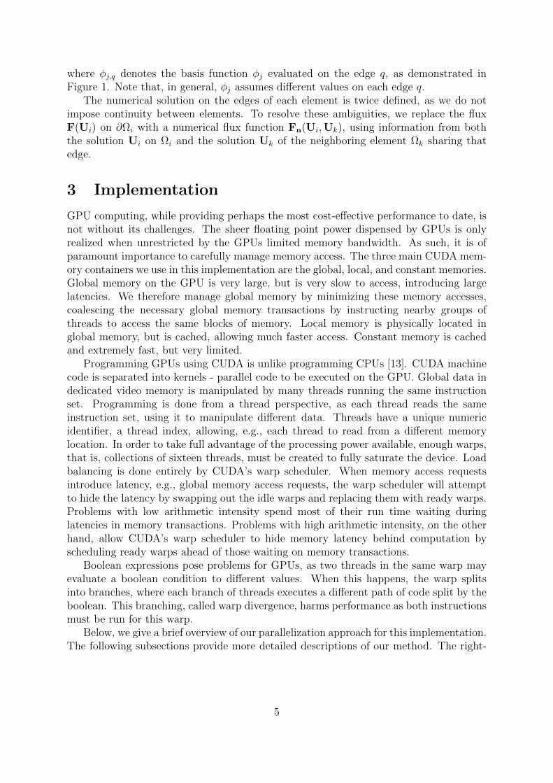
Figure 2: Storing the integration points on Ω0

(a) The integration points for the in-terior of Ω0, rk, stored in an array

b b

b

r1 r2 r3

(b) The boundary integration points for ∂Ω0, rq,k storedin an array

b b

b

bb

b

r2,1 r2,2

r3,1

r3,2r1,1

r1,2Ω0

r1,1 r1,2 r2,1 r2,2 r3,1 r3,2

hand side of equation (12) combines a volume integral∫Ω0

F(Ui) · (J−1i ∇φj) det Jidr (13)

and a surface integral

3∑q=1

∫I0

φj,qF(Ui) · ni,qli,q dξ (14)

consisting of three independent line integrals, for each j = 1, . . . , Np. Parallelization istherefore straightforward. As the volume integral contributions (13) for one element re-quire only local information from that element, i.e., the element’s coefficients and inverseJacobian, these contributions can be computed independently from each other. Simi-larly, each edge’s surface integral contributions (14) are computed independently as thesecomputations require local information from two elements sharing that edge, i.e., bothelements’ coefficients. An explicit integration scheme advances the solution coefficientsin time.

We use quadrature rules in [6] of order 2p to approximate the volume integral andthe Gauss-Legendre quadrature rules of order 2p+ 1 to approximate the surface integral.At each integration point rk in the interior of Ω0 shown in Figure 2a, we precomputethe values of φj(rk) and ∇φj(rk). We also precompute the values of φj(rq,k) at theintegration points rq,k on ∂Ω0, shown in Figure 2b, where q = 1, 2, 3 denotes which sideof the canonical triangle the integration points reside on. By storing these precomputedevaluations in GPU constant memory, we drastically reduce computation time.

3.1 Mesh Connectivity

Figure 3 shows an example of a simple mesh consisting of two elements. Elements Ω1

and Ω2 point to their respective edges; edges e1, . . . , e5 point back to their respectiveelements. Each edge stores two pointers: one each to its left and right elements, Ωl andΩr. We arbitrarily assign each of the two elements sharing an edge as either left or right.Edges lying on the boundary of the domain have only a left element and store a negative

6

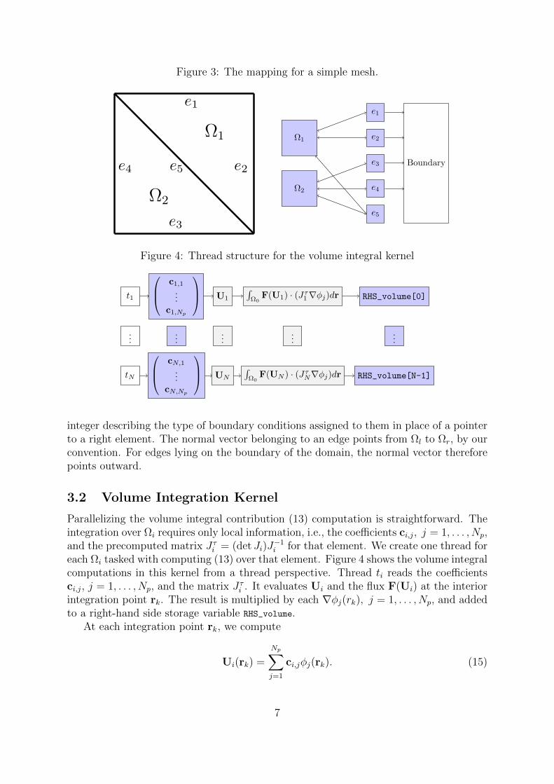
Figure 3: The mapping for a simple mesh.

Ω1

Ω2

e1

e2

e3

e4 e5

Ω1

Ω2

e1

e2

e3

e4

e5

Boundary

Figure 4: Thread structure for the volume integral kernel

t1

...

tN

c1,1

...c1,Np

... cN,1...

cN,Np

U1

...

UN

∫Ω0

F(U1) · (Jτ1∇φj)dr

...

∫Ω0

F(UN ) · (JτN∇φj)dr

RHS_volume[0]

...

RHS_volume[N-1]

integer describing the type of boundary conditions assigned to them in place of a pointerto a right element. The normal vector belonging to an edge points from Ωl to Ωr, by ourconvention. For edges lying on the boundary of the domain, the normal vector thereforepoints outward.

3.2 Volume Integration Kernel

Parallelizing the volume integral contribution (13) computation is straightforward. Theintegration over Ωi requires only local information, i.e., the coefficients ci,j, j = 1, . . . , Np,and the precomputed matrix Jτi = (det Ji)J

−1i for that element. We create one thread for

each Ωi tasked with computing (13) over that element. Figure 4 shows the volume integralcomputations in this kernel from a thread perspective. Thread ti reads the coefficientsci,j, j = 1, . . . , Np, and the matrix Jτi . It evaluates Ui and the flux F(Ui) at the interiorintegration point rk. The result is multiplied by each ∇φj(rk), j = 1, . . . , Np, and addedto a right-hand side storage variable RHS_volume.

At each integration point rk, we compute

Ui(rk) =

Np∑j=1

ci,jφj(rk). (15)

7

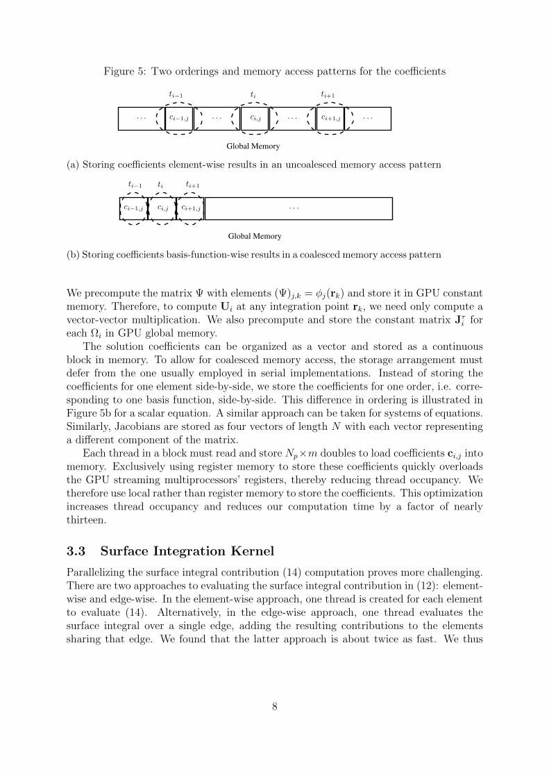
Figure 5: Two orderings and memory access patterns for the coefficients

ti−1 ti ti+1

ci−1,j ci,j ci+1,j

Global Memory

· · · · · · · · ·· · ·

(a) Storing coefficients element-wise results in an uncoalesced memory access pattern

ti−1 ti ti+1

ci−1,j ci,j ci+1,j

Global Memory

· · ·

(b) Storing coefficients basis-function-wise results in a coalesced memory access pattern

We precompute the matrix Ψ with elements (Ψ)j,k = φj(rk) and store it in GPU constantmemory. Therefore, to compute Ui at any integration point rk, we need only compute avector-vector multiplication. We also precompute and store the constant matrix Jτi foreach Ωi in GPU global memory.

The solution coefficients can be organized as a vector and stored as a continuousblock in memory. To allow for coalesced memory access, the storage arrangement mustdefer from the one usually employed in serial implementations. Instead of storing thecoefficients for one element side-by-side, we store the coefficients for one order, i.e. corre-sponding to one basis function, side-by-side. This difference in ordering is illustrated inFigure 5b for a scalar equation. A similar approach can be taken for systems of equations.Similarly, Jacobians are stored as four vectors of length N with each vector representinga different component of the matrix.

Each thread in a block must read and store Np×m doubles to load coefficients ci,j intomemory. Exclusively using register memory to store these coefficients quickly overloadsthe GPU streaming multiprocessors’ registers, thereby reducing thread occupancy. Wetherefore use local rather than register memory to store the coefficients. This optimizationincreases thread occupancy and reduces our computation time by a factor of nearlythirteen.

3.3 Surface Integration Kernel

Parallelizing the surface integral contribution (14) computation proves more challenging.There are two approaches to evaluating the surface integral contribution in (12): element-wise and edge-wise. In the element-wise approach, one thread is created for each elementto evaluate (14). Alternatively, in the edge-wise approach, one thread evaluates thesurface integral over a single edge, adding the resulting contributions to the elementssharing that edge. We found that the latter approach is about twice as fast. We thus

8

create one thread ti for each edge ei, shared by elements Ωl and Ωr to compute∫I0

φj,qFn(Ul,Ur)nili ds. (16)

The numerical flux function Fn(Ul,Ur) is identical in (16) for coefficients cl,j andcr,j. This function represents the most expensive computation in the surface integral,and we therefore structure our implementation to compute it only once for each edge.Additionally, the Jacobian (7) remains the same for both cl,j and cr,j, and the normalvector may be reused, as it points from the left to the right element.

While the numerical flux, the Jacobian, and the normal are the same, the final surfaceintegral contributions along an edge are not necessarily the same for cl,j and cr,j. As ourimplementation supports any unstructured triangular mesh, elements Ωl and Ωr may mapthe same edge to different sides of the canonical triangle. For example, Ωl may map edgeei to the side defined by (0, 0), (0,1), which we call s1, while Ωr maps that same edgeto the side defined by (1, 0), (0, 1), which we call s2. In this case, the basis functionevaluated on s1 is not equal to the same basis function evaluated on s2; refer to Figure 1.

We store two identifiers, L and R, for each edge ei to indicate which side of thecanonical triangle Ω0 that edge ei is mapped to by elements Ωl and Ωr, respectively.These identifiers, which we call side mappings, determine which side of the canonicaltriangle to evaluate the basis function on in (14). We therefore compute two separateintegrals in the same thread for edge ei, for each j = 1, . . . , Np. First, we compute∫

I0

φj,LFn(Ul,Ur)nili ds, (17)

for the surface integral contribution to cl,j, and then we compute∫I0

φj,RFn(Ul,Ur)(−ni)li ds, (18)

for the surface integral contribution to cr,j, where ni represents the normal vector pointingfrom Ωl to Ωr and li indicates the Jacobian given in (7). As discussed above, (17) is notnecessarily equal to (18), and two separate surface integrals must be computed for eachside.

Race conditions prevent us from simply adding the resulting surface integral contribu-tions together with the volume integrals for Ωl and Ωr as we compute them. For example,two threads assigned to two edges belonging to the same Ωi may compute their surfaceintegral contributions at the same time. When they both attempt to simultaneously addthat contribution to ci,j, that memory becomes corrupted. We attempted to use theatomicAdd operator, in order to bypass race conditions by serialising conflicting additionoperations in this kernel. Atomic operators are known, however, to significantly degradeperformance; in our implementation, runtime while using atomic operators increased bya factor of nine. In order to avoid using atomic operators, we chose instead to store eachterm separately in GPU global memory variables RHS_surface_left and RHS_surface_right

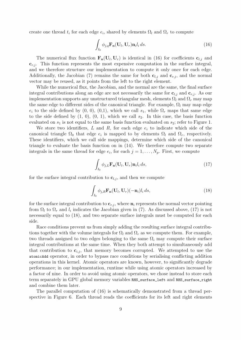
and combine them later.The parallel computation of (16) is schematically demonstrated from a thread per-

spective in Figure 6. Each thread reads the coefficients for its left and right elements

9

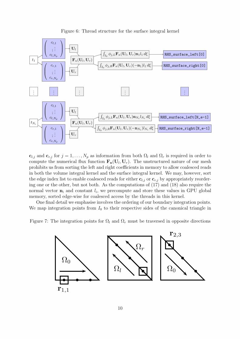
Figure 6: Thread structure for the surface integral kernel

t1

...

tNe

cl,1

;...

cl,Np

cr,1

;...

cr,Np

...

cl,1

;...

cl,Np

cr,1

;...

cr,Np

Ul

Ur

...

Ul

Ur

Fn(Ul,Ur)

Fn(Ul,Ur)

∫I0φj,LFn(Ul,Ur)n1l1 dξ

∫I0φj,RFn(Ul,Ur)(−n1)l1 dξ

...

∫I0φj,LFn(Ul,Ur)nNe

lNedξ

∫I0φj,RFn(Ul,Ur)(−nNe

)lNedξ

RHS_surface_left[0]

RHS_surface_right[0]

...

RHS_surface_left[N_e-1]

RHS_surface_right[N_e-1]

cl,j and cr,j for j = 1, . . . , Np as information from both Ωl and Ωr is required in order tocompute the numerical flux function Fn(Ul,Ur). The unstructured nature of our meshprohibits us from sorting the left and right coefficients in memory to allow coalesced readsin both the volume integral kernel and the surface integral kernel. We may, however, sortthe edge index list to enable coalesced reads for either cl,j or cr,j by appropriately reorder-ing one or the other, but not both. As the computations of (17) and (18) also require thenormal vector ni and constant li, we precompute and store these values in GPU globalmemory, sorted edge-wise for coalesced access by the threads in this kernel.

One final detail we emphasise involves the ordering of our boundary integration points.We map integration points from I0 to their respective sides of the canonical triangle in

Figure 7: The integration points for Ωl and Ωr must be traversed in opposite directions

b

b

b

b

b

b

b b b

r1,1

r2,3

Ωl

Ωr

Ω0

Ω0

10

a counter-clockwise direction, as illustrated in Figure 2b. The integration points mustbe traversed in opposite directions for Ωl and Ωr in order to reside in the same physicalspace, as shown in Figure 7. Thus, the flux evaluation at the k’th integration point is

Fn(Ul(rL,k),Ur(rR,2p+1−k)). (19)

We precompute three matrices (Ψq)j,k = φj(rq,k) for each side q = 1, 2, 3, of thecanonical triangle and store them row-by-row in a single, flattened array in GPU constantmemory. By using each edge’s two side mapping indices as an offset, we are able tolookup the correct integration points to use while avoiding boolean evaluations, whichwould create warp divergence.

If edge ei lies on a domain boundary, a ghost state Ug is created and assigned to Ur.We index our edges so that all boundary edges appear sorted and first in our edge list.This avoids warp divergence, as the boundary edges with boundaries of the same typewill be grouped in the same warp.

Each thread must read 2 × Np × m coefficients to compute Ul and Ur. Like inthe volume integral kernel, storing these coefficients in register memory would inhibitmaximum thread capacity. As such, we store both cl,j and cr,j in local memory.

3.4 Right-Hand Side Evaluator Kernel

The right-hand side evaluator kernel combines data from the three temporary storagevariables RHS_surface_left, RHS_surface_right, and RHS_volume from each Ωi to computethe right-hand side of equation (12). Each thread ti in the right-hand side evaluatorkernel combines the contributions from the surface and volume integrals for coefficientsci,j, j = 1, . . . , Np. For each edge of element Ωi, the thread must determine if that edgeconsiders element Ωi a left or right element. If the edge considers Ωi a left element,it reads from RHS_surface_left; on the other hand, if it considers Ωi a right element, itreads from RHS_surface_right. In either case, the thread reads from each j = 1, . . . , Np,appropriate memory location of the three temporary storage variables, combining themto form the right-hand side of (12).

As each thread must determine if Ωi is considered a left or a right element by eachof its edges, three boolean evaluations must be computed in this kernel. This introducesunavoidable warp divergence.

3.5 Limiting Kernel

We implement the Barth-Jespersen limiter [2] for linear p = 1 approximations. We aimto limit the maximum slope in the gradient of the scalar equation

Ui(r) = Ui + αi(∇Ui) · (r− r0), (20)

by selecting a limiting coefficient αi. In (20), Ui is the average value of Ui over Ωi and r0

is the coordinate of the centroid of Ω0. Limiting systems of equations involves finding aseparate αi for each variable in the system.

Suppose that element Ωi is surrounded by elements Ωa,Ωb, and Ωc, as shown in Figure8. We choose αi so that Ui introduces no new local extrema at the integration points on

11

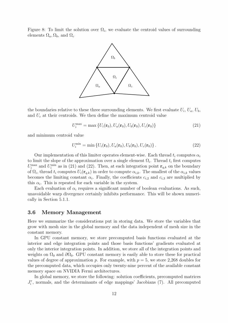
Figure 8: To limit the solution over Ωi, we evaluate the centroid values of surroundingelements Ωa,Ωb, and Ωc

b

b

b

ΩcΩa

Ωi

Ωb

the boundaries relative to these three surrounding elements. We first evaluate Ui, Ua, Ub,and Uc at their centroids. We then define the maximum centroid value

Umaxi = max Ui(r0), Ua(r0), Ub(r0), Uc(r0) (21)

and minimum centroid value

Umini = min Ui(r0), Ua(r0), Ub(r0), Uc(r0) . (22)

Our implementation of this limiter operates element-wise. Each thread ti computes αito limit the slope of the approximation over a single element Ωi. Thread ti first computesUmaxi and Umin

i as in (21) and (22). Then, at each integration point rq,k on the boundaryof Ωi, thread ti computes Ui(rq,k) in order to compute αi,k. The smallest of the αi,k valuesbecomes the limiting constant αi. Finally, the coefficients ci,2 and ci,3 are multiplied bythis αi. This is repeated for each variable in the system.

Each evaluation of αi requires a significant number of boolean evaluations. As such,unavoidable warp divergence certainly inhibits performance. This will be shown numeri-cally in Section 5.1.1.

3.6 Memory Management

Here we summarize the considerations put in storing data. We store the variables thatgrow with mesh size in the global memory and the data independent of mesh size in theconstant memory.

In GPU constant memory, we store precomputed basis functions evaluated at theinterior and edge integration points and those basis functions’ gradients evaluated atonly the interior integration points. In addition, we store all of the integration points andweights on Ω0 and ∂Ω0. GPU constant memory is easily able to store these for practicalvalues of degree of approximation p. For example, with p = 5, we store 2,268 doubles forthe precomputed data, which occupies only twenty-nine percent of the available constantmemory space on NVIDIA Fermi architectures.

In global memory, we store the following: solution coefficients, precomputed matricesJτi , normals, and the determinants of edge mappings’ Jacobians (7). All precomputed

12

data is appropriately sorted element-wise or edge-wise to allow coalesced reads as dis-cussed in Sections 3.2 and 3.3.

The total memory required for computation depends on four factors. First, the sizeof the mesh N determines the number of elements and edges, as we store the elementvertices in GPU global memory. Second, the degree of the polynomial approximation Np

determines the number of coefficients required to approximate the solution. Third, thesize of the system, m, requires a vector of solution coefficients for each variable in thatsystem. For each element, we require m×Np coefficients to represent the approximatedsolution over that element. Finally, the ODE solver typically needs extra storage variablesfor intermediate steps or stages, which must be stored in global memory.

4 Computed Examples

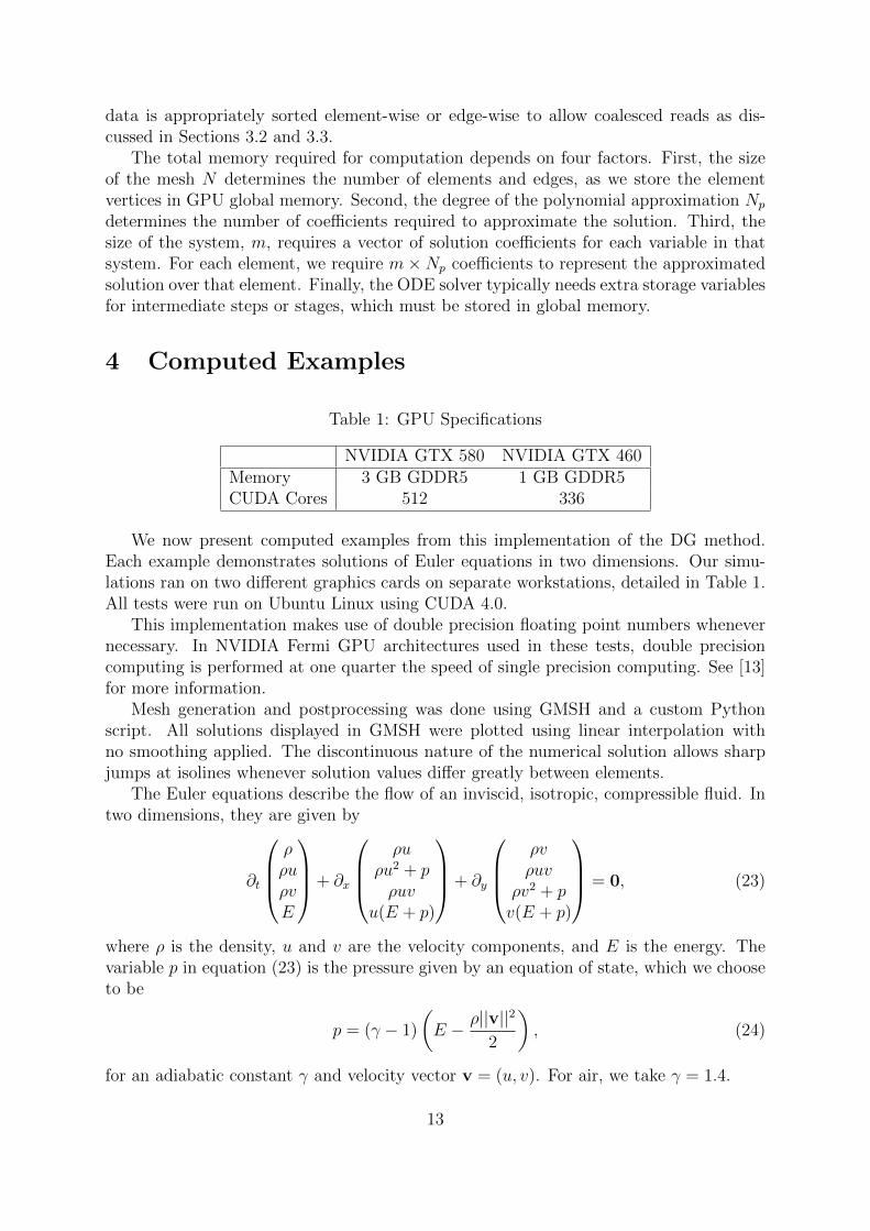
Table 1: GPU Specifications

NVIDIA GTX 580 NVIDIA GTX 460Memory 3 GB GDDR5 1 GB GDDR5CUDA Cores 512 336

We now present computed examples from this implementation of the DG method.Each example demonstrates solutions of Euler equations in two dimensions. Our simu-lations ran on two different graphics cards on separate workstations, detailed in Table 1.All tests were run on Ubuntu Linux using CUDA 4.0.

This implementation makes use of double precision floating point numbers whenevernecessary. In NVIDIA Fermi GPU architectures used in these tests, double precisioncomputing is performed at one quarter the speed of single precision computing. See [13]for more information.

Mesh generation and postprocessing was done using GMSH and a custom Pythonscript. All solutions displayed in GMSH were plotted using linear interpolation withno smoothing applied. The discontinuous nature of the numerical solution allows sharpjumps at isolines whenever solution values differ greatly between elements.

The Euler equations describe the flow of an inviscid, isotropic, compressible fluid. Intwo dimensions, they are given by

∂t

ρρuρvE

+ ∂x

ρu

ρu2 + pρuv

u(E + p)

+ ∂y

ρvρuv

ρv2 + pv(E + p)

= 0, (23)

where ρ is the density, u and v are the velocity components, and E is the energy. Thevariable p in equation (23) is the pressure given by an equation of state, which we chooseto be

p = (γ − 1)

(E − ρ||v||2

2

), (24)

for an adiabatic constant γ and velocity vector v = (u, v). For air, we take γ = 1.4.

13

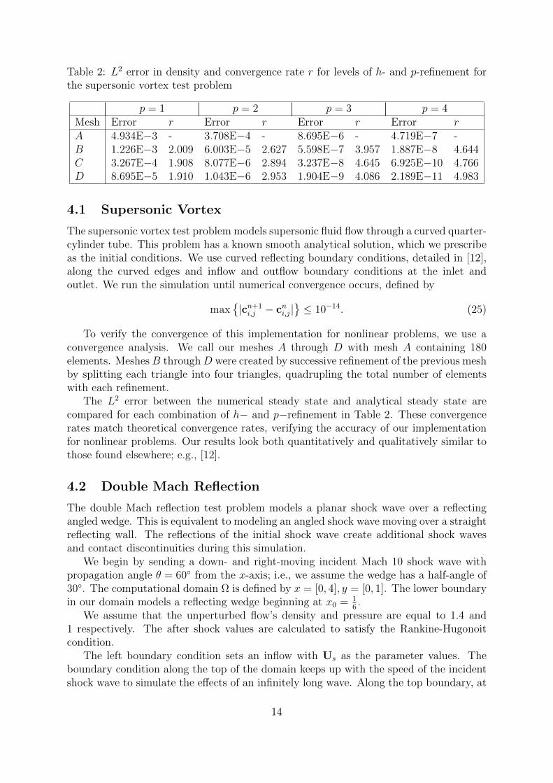
Table 2: L2 error in density and convergence rate r for levels of h- and p-refinement forthe supersonic vortex test problem

p = 1 p = 2 p = 3 p = 4Mesh Error r Error r Error r Error rA 4.934E−3 - 3.708E−4 - 8.695E−6 - 4.719E−7 -B 1.226E−3 2.009 6.003E−5 2.627 5.598E−7 3.957 1.887E−8 4.644C 3.267E−4 1.908 8.077E−6 2.894 3.237E−8 4.645 6.925E−10 4.766D 8.695E−5 1.910 1.043E−6 2.953 1.904E−9 4.086 2.189E−11 4.983

4.1 Supersonic Vortex

The supersonic vortex test problem models supersonic fluid flow through a curved quarter-cylinder tube. This problem has a known smooth analytical solution, which we prescribeas the initial conditions. We use curved reflecting boundary conditions, detailed in [12],along the curved edges and inflow and outflow boundary conditions at the inlet andoutlet. We run the simulation until numerical convergence occurs, defined by

max|cn+1i,j − cni,j|

≤ 10−14. (25)

To verify the convergence of this implementation for nonlinear problems, we use aconvergence analysis. We call our meshes A through D with mesh A containing 180elements. MeshesB throughD were created by successive refinement of the previous meshby splitting each triangle into four triangles, quadrupling the total number of elementswith each refinement.

The L2 error between the numerical steady state and analytical steady state arecompared for each combination of h− and p−refinement in Table 2. These convergencerates match theoretical convergence rates, verifying the accuracy of our implementationfor nonlinear problems. Our results look both quantitatively and qualitatively similar tothose found elsewhere; e.g., [12].

4.2 Double Mach Reflection

The double Mach reflection test problem models a planar shock wave over a reflectingangled wedge. This is equivalent to modeling an angled shock wave moving over a straightreflecting wall. The reflections of the initial shock wave create additional shock wavesand contact discontinuities during this simulation.

We begin by sending a down- and right-moving incident Mach 10 shock wave withpropagation angle θ = 60 from the x-axis; i.e., we assume the wedge has a half-angle of30. The computational domain Ω is defined by x = [0, 4], y = [0, 1]. The lower boundaryin our domain models a reflecting wedge beginning at x0 = 1

6.

We assume that the unperturbed flow’s density and pressure are equal to 1.4 and1 respectively. The after shock values are calculated to satisfy the Rankine-Hugonoitcondition.

The left boundary condition sets an inflow with Us as the parameter values. Theboundary condition along the top of the domain keeps up with the speed of the incidentshock wave to simulate the effects of an infinitely long wave. Along the top boundary, at

14

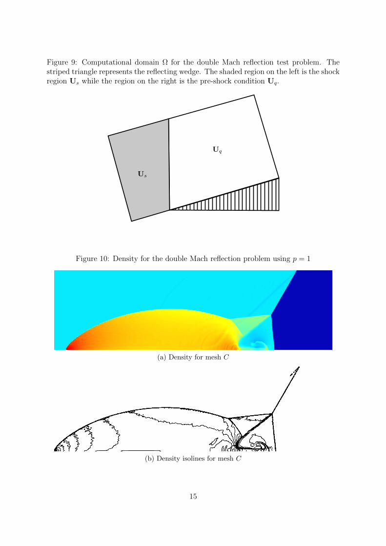
Figure 9: Computational domain Ω for the double Mach reflection test problem. Thestriped triangle represents the reflecting wedge. The shaded region on the left is the shockregion Us while the region on the right is the pre-shock condition Uq.

Us

Uq

Figure 10: Density for the double Mach reflection problem using p = 1

(a) Density for mesh C

(b) Density isolines for mesh C

15

Table 3: Performance of the double Mach reflection test problem

Mesh Elements Memory GTX 460 Runtime (min) GTX 580 Runtime (min)A 68,622 43.64 MB 1.74 0.81B 236,964 176.48 MB 21.19 9.78C 964,338 717.82 MB 165.82 76.51

integration points to the left of the shock wave, the exact values from Us are prescribed,while points to right of the shock wave use the values from Uq. The lower boundarycondition prescribes the values of the shock Us at x ≤ x0 and uses reflecting boundaryconditions beyond to simulate a perfectly reflecting wedge.

Our test set runs over three unstructured, triangular meshes of varying mesh sizes,reported in Table 3. We compute the solution until t = 0.2 when the shock has movednearly across the entire domain. Our solution is computed using p = 1 linear polynomialswith the slopes limited using the Barth-Jespersen limiter. Mesh refinement is done bysetting a smaller maximum edge length and creating a new mesh with GMSH.

The density and density isolines at t = 0.2 for the most refined mesh, C, are plotted inFigure 10. Our jet stream travels and expands as in similar simulations in [4]. The exactboundary condition at the top edge of our domain introduces small numerical artifactswhich can be seen at the front and top of the shock.

Table 3 also reports total runtime for both GPUs used and memory costs for thesesimulations using the classical second-order Runge-Kutta time integration scheme. Thesimulation time, even for the very large meshes, is not prohibitive. Meshes of C’s size aretypically too large to be run in serial implementations, usually requiring supercomputingtime. In contrast, the GTX 580 completed this simulation in just over an hour.

5 Benchmarks

We now present our benchmarks of this implementation. First, we demonstrate thespeedup when compared with a single-core, serial implementation. Then, we examinethe performance degradation introduced by our limiter. Finally, we show how our imple-mentation scales with mesh sizes. In all tests following, we use the classical fourth-orderRunge-Kutta time integration scheme.

5.1 Serial Comparison on a CPU

We compare the performance of this implementation with a CPU implementation com-puting in serial. To create the serial implementation, we rewrote the GPU implementationin C, making the following necessary adjustments. We replace every parallel computa-tion run by a thread with a for loop. We also replace all GPU memory allocation withCPU memory allocations. In addition, we change the memory access pattern in the CPUimplementation so that the coefficients are located nearby each other from an elementperspective as opposed to a thread perspective. Finally, we remove all unnecessary mem-ory copies as we no longer transfer data between the GPU and CPU. The surface integralcontributions are still computed separately from the volume integral contributions and

16

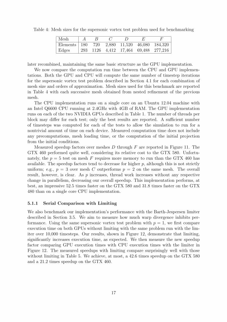
Table 4: Mesh sizes for the supersonic vortex test problem used for benchmarking

Mesh A B C D E FElements 180 720 2,880 11,520 46,080 184,320Edges 293 1126 4,412 17,464 69,488 277,216

later recombined, maintaining the same basic structure as the GPU implementation.We now compare the computation run time between the CPU and GPU implemen-

tations. Both the GPU and CPU will compute the same number of timestep iterationsfor the supersonic vortex test problem described in Section 4.1 for each combination ofmesh size and orders of approximation. Mesh sizes used for this benchmark are reportedin Table 4 with each successive mesh obtained from nested refinement of the previousmesh.

The CPU implementation runs on a single core on an Ubuntu 12.04 machine withan Intel Q6600 CPU running at 2.4GHz with 4GB of RAM. The GPU implementationruns on each of the two NVIDIA GPUs described in Table 1. The number of threads perblock may differ for each test; only the best results are reported. A sufficient numberof timesteps was computed for each of the tests to allow the simulation to run for anontrivial amount of time on each device. Measured computation time does not includeany precomputations, mesh loading time, or the computation of the initial projectionfrom the initial conditions.

Measured speedup factors over meshes D through F are reported in Figure 11. TheGTX 460 performed quite well, considering its relative cost to the GTX 580. Unfortu-nately, the p = 5 test on mesh F requires more memory to run than the GTX 460 hasavailable. The speedup factors tend to decrease for higher p, although this is not strictlyuniform; e.g., p = 3 over mesh C outperforms p = 2 on the same mesh. The overallresult, however, is clear. As p increases, thread work increases without any respectivechange in parallelism, decreasing our overall speedup. This implementation performs, atbest, an impressive 52.5 times faster on the GTX 580 and 31.8 times faster on the GTX480 than on a single core CPU implementation.

5.1.1 Serial Comparison with Limiting

We also benchmark our implementation’s performance with the Barth-Jespersen limiterdescribed in Section 3.5. We aim to measure how much warp divergence inhibits per-formance. Using the same supersonic vortex test problem with p = 1, we first compareexecution time on both GPUs without limiting with the same problem run with the lim-iter over 10,000 timesteps. Our results, shown in Figure 12, demonstrate that limiting,significantly increases execution time, as expected. We then measure the new speedupfactor comparing GPU execution times with CPU execution times with the limiter inFigure 12. The measured speedups with limiting compare surprisingly well with thosewithout limiting in Table 5. We achieve, at most, a 42.6 times speedup on the GTX 580and a 21.2 times speedup on the GTX 460.

17

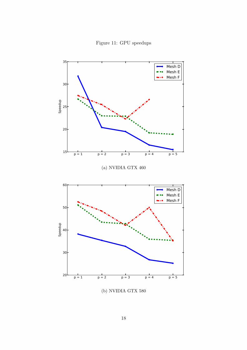
Figure 11: GPU speedups

p = 1 p = 2 p = 3 p = 4 p = 515

20

25

30

35Speedup

Mesh DMesh EMesh F

(a) NVIDIA GTX 460

p = 1 p = 2 p = 3 p = 4 p = 520

30

40

50

60

Speedup

Mesh DMesh EMesh F

(b) NVIDIA GTX 580

18

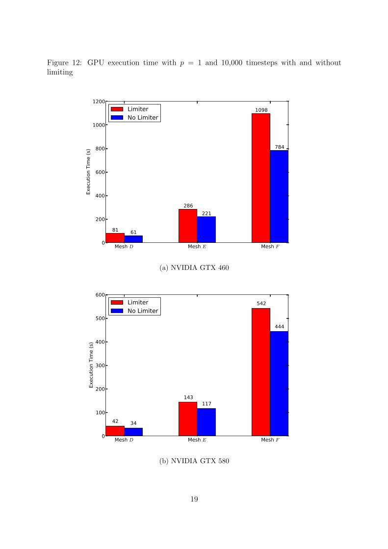
Figure 12: GPU execution time with p = 1 and 10,000 timesteps with and withoutlimiting

Mesh D Mesh E Mesh F0

200

400

600

800

1000

1200

Execu

tion T

ime (

s)

81

286

1098

61

221

784

LimiterNo Limiter

(a) NVIDIA GTX 460

Mesh D Mesh E Mesh F0

100

200

300

400

500

600

Execu

tion T

ime (

s)

42

143

542

34

117

444

LimiterNo Limiter

(b) NVIDIA GTX 580

19

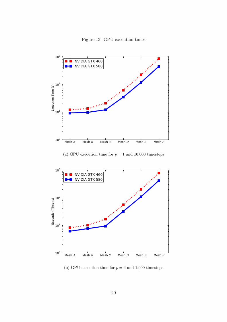
Figure 13: GPU execution times

Mesh A Mesh B Mesh C Mesh D Mesh E Mesh F100

101

102

103

Execu

tion T

ime (

s)

NVIDIA GTX 460NVIDIA GTX 580

(a) GPU execution time for p = 1 and 10,000 timesteps

Mesh A Mesh B Mesh C Mesh D Mesh E Mesh F100

101

102

103

Execu

tion T

ime (

s)

NVIDIA GTX 460NVIDIA GTX 580

(b) GPU execution time for p = 4 and 1,000 timesteps

20

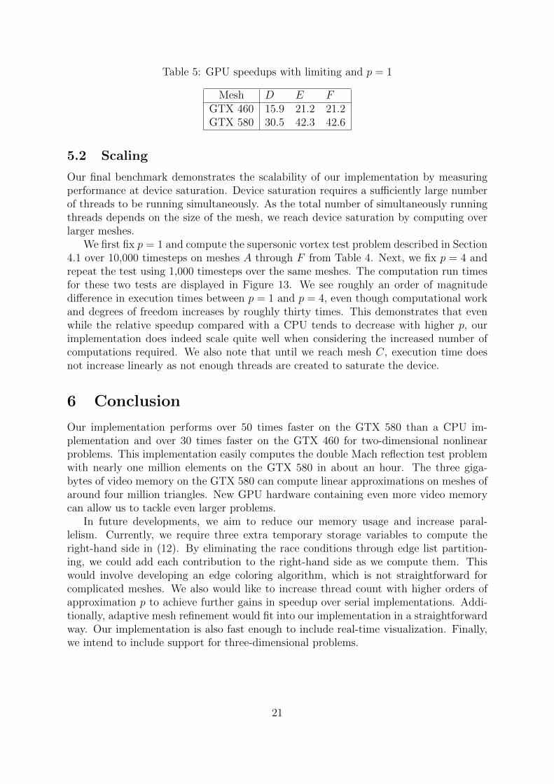
Table 5: GPU speedups with limiting and p = 1

Mesh D E FGTX 460 15.9 21.2 21.2GTX 580 30.5 42.3 42.6

5.2 Scaling

Our final benchmark demonstrates the scalability of our implementation by measuringperformance at device saturation. Device saturation requires a sufficiently large numberof threads to be running simultaneously. As the total number of simultaneously runningthreads depends on the size of the mesh, we reach device saturation by computing overlarger meshes.

We first fix p = 1 and compute the supersonic vortex test problem described in Section4.1 over 10,000 timesteps on meshes A through F from Table 4. Next, we fix p = 4 andrepeat the test using 1,000 timesteps over the same meshes. The computation run timesfor these two tests are displayed in Figure 13. We see roughly an order of magnitudedifference in execution times between p = 1 and p = 4, even though computational workand degrees of freedom increases by roughly thirty times. This demonstrates that evenwhile the relative speedup compared with a CPU tends to decrease with higher p, ourimplementation does indeed scale quite well when considering the increased number ofcomputations required. We also note that until we reach mesh C, execution time doesnot increase linearly as not enough threads are created to saturate the device.

6 Conclusion

Our implementation performs over 50 times faster on the GTX 580 than a CPU im-plementation and over 30 times faster on the GTX 460 for two-dimensional nonlinearproblems. This implementation easily computes the double Mach reflection test problemwith nearly one million elements on the GTX 580 in about an hour. The three giga-bytes of video memory on the GTX 580 can compute linear approximations on meshes ofaround four million triangles. New GPU hardware containing even more video memorycan allow us to tackle even larger problems.

In future developments, we aim to reduce our memory usage and increase paral-lelism. Currently, we require three extra temporary storage variables to compute theright-hand side in (12). By eliminating the race conditions through edge list partition-ing, we could add each contribution to the right-hand side as we compute them. Thiswould involve developing an edge coloring algorithm, which is not straightforward forcomplicated meshes. We also would like to increase thread count with higher orders ofapproximation p to achieve further gains in speedup over serial implementations. Addi-tionally, adaptive mesh refinement would fit into our implementation in a straightforwardway. Our implementation is also fast enough to include real-time visualization. Finally,we intend to include support for three-dimensional problems.

21

7 Acknowledgment

This research was supported in part by Natural Sciences and Engineering Research Coun-cil (NSERC) of Canada grant 341373-07.

Bibliography

[1] V.G. Asouti, X. S. Trompoukis, I. C. Kampolis, and K. C. Giannakoglou. UnsteadyCFD computations using vertex-centered finite volumes for unstructured grids ongraphics processing units. International Journal for Numerical Methods in Fluids,67(2):232–246, 2011.

[2] T.J. Barth and D.C. Jespersen. The design and application of upwind schemes onunstructured meshes. In 27th Aerospace Sciences Meeting, AIAA 89-0366, Reno,Nevada, 1989.

[3] T. Brandvik and G. Pullan. Acceleration of a two-dimensional Euler flow solverusing commodity graphics hardware. Proceedings of the Institution of MechanicalEngineers, Part C: Journal of Mechanical Engineering Science, 221(12):1745–1748,2007.

[4] B. Cockburn, G. Karniadakis, and C. W. Shu. The development of discontinuousGalerkin methods. 1999.

[5] A. Corrigan, F. Camelli, R. Lohner, and J. Wallin. Running unstructured grid basedCFD solvers on modern graphics hardware. AIAA paper, 4001:22–25, 2009.

[6] D. A. Dunavant. High degree efficient symmetrical Gaussian quadrature rules for thetriangle. International Journal for Numerical Methods in Engineering, 21(6):1129–1148, 1985.

[7] N. Goedel, T. Warburton, and M. Clemens. GPU accelerated discontinuous GalerkinFEM for electromagnetic radio frequency problems. Antennas and Propagation So-ciety International Symposium, pages 1–4, 2009.

[8] J. S Hesthaven, J. Bridge, N. Goedel, A. Klockner, and T. Warburton. Nodaldiscontinuous Galerkin methods on graphics processing units (GPUs).

[9] A. Klockner, T. Warburton, and J. S. Hesthaven. Nodal discontinuous Galerkinmethods on graphics processors. Journal of Computational Physics, 228(21):7863–7882, 2009.

[10] A. Klockner, T. Warburton, and J. S. Hesthaven. High-order discontinuous Galerkinmethods by GPU metaprogramming. GPU Solutions to Multi-scale Problems inScience and Engineering, 2012.

[11] T. Koornwinder. Two-variable analogues of the classical orthogonal polynomials. Intheory and applications of special functions. Academic Press, 1975.

22

[12] L. Krivodonova and M. Berger. High-order accurate implementation of solid wallboundary conditions in curved geometries. Journal of Computational Physics,211:492–512, 2006.

[13] NVIDIA. NVIDIA CUDA C Programming Guide 4.2. NVIDIA Corporation, SantaClara, USA, June, 2013.

23