Embed Size (px)
Citation preview
Vol.:(0123456789)
Discover Internet of Things (2021) 1:11 | https://doi.org/10.1007/s43926-021-00011-w
1 3
Discover Internet of Things
Research
Bayesian Topology Learning and noise removal from network data
Mahmoud Ramezani Mayiami1 · Mohammad Hajimirsadeghi2 · Karl Skretting3 · Xiaowen Dong4 · Rick S. Blum2 · H. Vincent Poor5
Received: 4 February 2021 / Accepted: 10 March 2021 © The Author(s) 2021 OPEN
AbstractLearning the topology of a graph from available data is of great interest in many emerging applications. Some examples are social networks, internet of things networks (intelligent IoT and industrial IoT), biological connection networks, sen-sor networks and traffic network patterns. In this paper, a graph topology inference approach is proposed to learn the underlying graph structure from a given set of noisy multi-variate observations, which are modeled as graph signals generated from a Gaussian Markov Random Field (GMRF) process. A factor analysis model is applied to represent the graph signals in a latent space where the basis is related to the underlying graph structure. An optimal graph filter is also developed to recover the graph signals from noisy observations. In the final step, an optimization problem is proposed to learn the underlying graph topology from the recovered signals. Moreover, a fast algorithm employing the proximal point method has been proposed to solve the problem efficiently. Experimental results employing both synthetic and real data show the effectiveness of the proposed method in recovering the signals and inferring the underlying graph.
Keywords Graph signal processing · Topology learning · Signal representation · Bayesian inference · Internet of things
1 Introduction
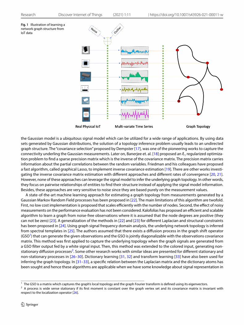
Many applications including internet of things (IoT) networks, sensor networks, social networks, gene networks, customer consumption data in utility companies, financial data, regional temperature data, and brain computer interface meas-urements result in rapidly growing data volumes. IoT networks are a rapidly emerging technology where smart sensors are connected to easily enable data collection anywhere and anytime [1]. Figure 1 illustrates how an IoT network may involve collecting large volume of multi-variate time series data which are connected in some abstract senses.
Storing and analyzing these huge data volumes is challenging due to the need for high computation and power resources. The emerging field of graph signal processing (GSP) [2, 3] simplifies the analysis of large data volumes by the use of graph theory, where each graph node represents a component of the system. Several applications can be analyzed by graphs, which can capture the underlying topology among different entities of the network. For example, a network of thermal sensors which measures temperatures in different regions, can be modeled by a graph.
In some cases, the graph topology is not known a priori. Thus, one of the desired goals of the GSP framework is esti-mating the underlying topology given a set of measured data. Some researches concentrated on directed topology estimation [4–16], where specific process models have been used which are suitable for limited applications. However,
* Mahmoud Ramezani Mayiami, [email protected]; Mohammad Hajimirsadeghi, [email protected]; Karl Skretting, [email protected]; Xiaowen Dong, [email protected]; Rick S. Blum, [email protected]; H. Vincent Poor, [email protected] | 1Department of ICT, University of Agder, Grimstad, Norway. 2Department of ECE, Lehigh University, Bethlehem, USA. 3Department of EECS, University of Stavanger, Stavanger, Norway. 4Department of Engineering Science, University of Oxford, Oxford, UK. 5Department of Electrical Engineering, Princeton University, Princeton, USA.
Vol:.(1234567890)
Research Discover Internet of Things (2021) 1:11 | https://doi.org/10.1007/s43926-021-00011-w
1 3
the Gaussian model is a ubiquitous signal model which can be utilized for a wide range of applications. By using data sets generated by Gaussian distributions, the solution of a topology inference problem usually leads to an undirected graph structure. The “covariance selection” proposed by Dempster [17], was one of the pioneering works to capture the connectivity underling the Gaussian measurements. Later on, Banerjee et. al. [18] proposed an ℓ1 regularized optimiza-tion problem to find a sparse precision matrix which is the inverse of the covariance matrix. The precision matrix carries information about the partial correlations between the random variables. Friedman and his colleagues have proposed a fast algorithm, called graphical Lasso, to implement inverse covariance estimation [19]. There are other works investi-gating the inverse covariance matrix estimation with different approaches and different rates of convergence [20, 21]. However, none of these approaches can leverage the signal model to infer the underlying graph topology. In other words, they focus on pairwise relationships of entities to find their structure instead of applying the signal model information. Besides, these approaches are very sensitive to noise since they are based purely on the measurement values.
A state-of-the-art machine learning approach for estimating a graph topology from measurements generated by a Gaussian Markov Random Field processes has been proposed in [22]. The main limitations of this algorithm are twofold. First, no low cost implementation is proposed that scales efficiently with the number of nodes. Second, the effect of noisy measurements on the performance evaluation has not been considered. Kalofolias has proposed an efficient and scalable algorithm to learn a graph from noise-free observations where it is assumed that the node degrees are positive (they can not be zero) [23]. A generalization of the methods in [22] and [23] for different Laplacian and structural constraints has been proposed in [24]. Using graph signal frequency domain analysis, the underlying network topology is inferred from spectral templates in [25]. The authors assumed that there exists a diffusion process in the graph shift operator (GSO1) that can generate the given observations and the GSO is jointly diagonalizable with the observations covariance matrix. This method was first applied to capture the underlying topology when the graph signals are generated from a GSO filter output fed by a white signal input. Then, this method was extended to the colored input, generating non-stationary diffusion processes2. Some other research works with similar ideas are presented for different stationary and non-stationary processes in [26–30]. Dictionary learning [31, 32] and transform learning [33] have also been used for inferring the graph topology. In [31–33], a specific relation between the Laplacian matrix and the dictionary atoms has been sought and hence these algorithms are applicable when we have some knowledge about signal representation in
Fig. 1 Illustration of learning a network graph structure from IoT data
1 The GSO is a matrix which captures the graph’s local topology and the graph Fourier transform is defined using its eigenvectors.2 A process is wide sense stationary if its first moment is constant over the graph vertex set and its covariance matrix is invariant with respect to the localization operator [26].
Vol.:(0123456789)
Discover Internet of Things (2021) 1:11 | https://doi.org/10.1007/s43926-021-00011-w Research
1 3
the transform domain. There are also many other papers investigating the topology identification and graph learning methods from different perspectives [8, 34–43]. However, none of the above approaches has discussed graph signal recovery and topology learning when the measurements are corrupted by noise.
The inexpensive sensors found in a wide variety of applications distort the observed data samples. The resulting measurement errors in the data analysis are conventionally modeled as noise [44] and it is generally desirable to remove this noise in many applications [45, 46], which generally produced a more accurate learned topology. In a recent research [47], Liu and her colleagues proposed a noisy data cleansing algorithm to remove unwanted distortion from Industrial IoT (IIoT) sensor data in manufacturing. They showed the efficiency of their proposed method on the multi-variate time-series data collected from a real IIoT based four stage compressor manufacturing plant. In [48], the effect of distortion on the trading data has been discussed, where the stock market’s impact on this data is characterized by a graph [49]. There are also other studies in the GSP framework considering the noise effect on the observations, e.g. [50], but they assumed that they have knowledge about the underlying graph and did not tackle graph topology inference and noise removal at the same time. While it is a naive strategy to find the graph topology first and then remove the noise from the graph signal, this approach has a low performance due to the accumulation of errors in topology learning and signal estimation.
To solve this type of problem in a topology learning framework, an optimization problem is usually formulated with at least two objective terms. The first term is always a data fidelity term controlling the energy of the signal recovery error. The second term takes care of the graph signal smoothness over the learned topology. A smooth signal has smooth variations on the underlying topology, or in other words, connected nodes in the estimated structure have similar signal values. To overcome over-fitting, the data fidelity term is regularized by a smoothing term and an exhaustive search is applied to find the regularization parameter. In many applications, the relationship between the noise variance and the regularization parameters may be held directly, e.g. image restoration [51]. Thus, estimating the noise variance not only provides a cleaner version of the signal for further analysis, but also helps to overcome the overfitting problem. All things considered, the estimation of noise variance is the main step to design the filter for smoothing the signal and denoising the given measurements.
It is usually assumed that the measurement noise has a zero mean Gaussaian distribution model which is independent of the desired signal. Thus, finding the noise variance is of interest to design a filter for signal denoising. The noise variance estimation is not only useful from a signal recovery perspective, it is also important from a graph learning point of view. Since finding the underlying structure from a noise-free data set is more accurate than from noisy graph signals, signal denoising can contribute to estimating a more accurate graph topology. In this respect, Chepuri et al. [52] proposed an approach to find the connectivity graph and remove noise from measurements. They proposed a non-convex, cardinal-ity constrained, boolean optimization problem along with a convex relaxation. They have assumed that the number of edges is known in advance and the proposed method scales with the desired number of edges. Another approach has been proposed in [53], which estimates the topology and removes the noise from the measured signals, simultaneously. They adopted a factor analysis model for the multi-variate signals and imposed a Gaussian prior on the latent variables that control the graph signals. By applying a Bayesian framework, the maximum a posteriori (MAP) probability estimate of the latent variable is investigated. Considering signal smoothness over the underlying graph, this procedure leads to an optimization problem over the graph topology and graph signals, simultaneously. A limitation of this approach is that an exhaustive search is applied to find the regularization parameter or noise variance which is not very suitable, especially for the situation in which the measurement noise varies over time.
Our contribution Given a set of noisy multi-variate signal measurements, we propose a new algorithm to perform the underlying topology learning and graph signal noise removal. This graph topology characterizes the affinity relation-ship among the multi-variate signals. We have proposed a minimum mean square error estimation (MMSE) approach for signal recovery and topology learning and unlike [53], we estimate the regularization parameters analytically rather than by using a grid search. We show that the regularization parameters are linked to the noise variance which is usually unknown, and hence, finding the noise variance helps adjusting the parameters precisely. Besides, it is the main role in designing a filter to denoise the graph measurements. In other words, to compare the current paper with other similar ones, especially [53], two specific points must be considered; (1) understanding the relation between amount of noise and the regularization parameters in the denoising procedure, and (2) a rigorous strategy to estimate the noise variance instead of assuming that it is known in advance. The MMSE procedure is utilized to estimate the optimal Laplacian matrix, whose eigenvalue matrix is the precision matrix of the Gaussian Markov Random Field process. This work is an extension of our previous paper [54], in which we studied the problem of joint graph signal recovery and topology learning using an off-the-shelf optimization toolbox to implement the algorithm. However, in this version, we propose a fast algorithm and prove its convergence analytically. Moreover, we provide simulation results on real world data sets in this paper. To
Vol:.(1234567890)
Research Discover Internet of Things (2021) 1:11 | https://doi.org/10.1007/s43926-021-00011-w
1 3
compare the results with the state of the art methods, we applied some measures which evaluate the performances from two distinct perspectives which are signal recovery error and graph topology estimation accuracy. Therefore, we can compare our proposed method against other methods that employ signal denoising strategies, like the one proposed in [24]. A simple graph filter is applied based on the estimated noise variance which can be used in many multi-variate measurements applications, including industrial internet of things IIoT applications. In the preprocessing stage in some IIoT applications, it is necessary to denoise the measurements, remove outlier data, detect anomalies, and estimate the missing values of some data. By the proposed method, the knowledge of the underlying data structure can be applied to implement all of these tasks. As an application of our idea in the area of IIoT networks, we apply our proposed method to estimated the missing values of sensor readings for a power consumption dataset.
The rest of the paper is organized as follows; in Sect. 2, some preliminaries about graph theory and signal process-ing on graphs are presented. Section 3 formulates the graph topology learning problem via a Bayesian framework and proposes a general algorithm for implementation, called Bayesian Topology Learning (BTL). In Sect. 4, a method is pro-posed to implement BTL efficiently via solving a proximal point algorithm, called BTL-PPA. The proof of convergence is also presented in Sect. 5. Section 6 presents experimental results obtained from the proposed method for temperature sensor networks and IIoT applications by using both real and synthetically simulated data. Finally, the Sect. 7 concludes the paper. Throughout the paper, lowercase regular letters, lowercase bold letters, and uppercase bold letters denote scalars, vectors, and matrices, respectively. The rest of the notation is presented in Table 1.
2 Background on graph signal processing
Let G = (V, E,�) to be a graph with the vertices vi ∈ V , the edge set E , and the undirected weight matrix � . Each edge (vi, vj), 1 ≤ i, j ≤ N has a weight of wij in the corresponding entry of � ∈ ℝ
N×N+
. Thus, wij = 0 implies no connection and wij = wji > 0 quantifies the strength of connection between the node vi and the node vj . For simplicity of presenta-tion, we assume that the diagonal entries of the weight matrix are zero, i.e. there is no self loop. The adjacency matrix
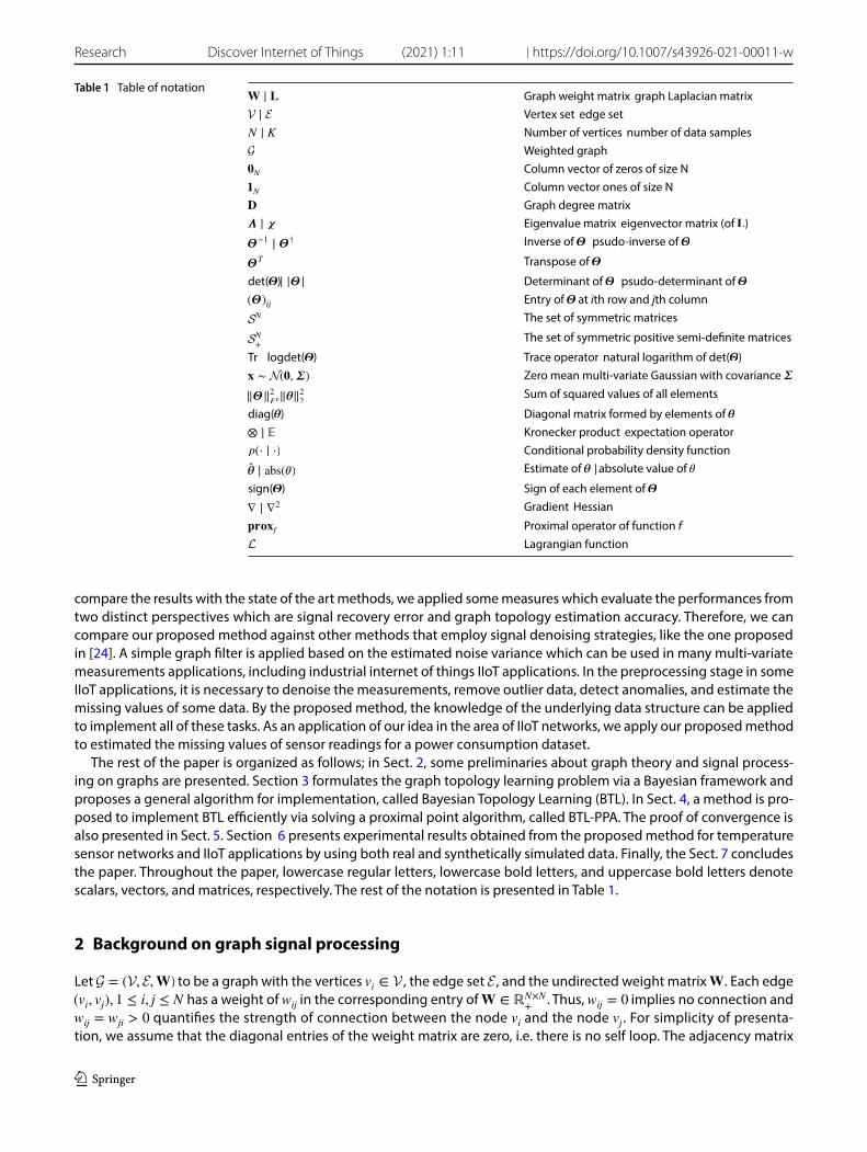
Table 1 Table of notation� ∣ � Graph weight matrix graph Laplacian matrixV ∣ E Vertex set edge setN ∣ K Number of vertices number of data samplesG Weighted graph�N Column vector of zeros of size N�N Column vector ones of size N� Graph degree matrix� ∣ � Eigenvalue matrix eigenvector matrix (of �)
�−1 ∣ �† Inverse of � psudo-inverse of �
�T Transpose of �
det(�)∣ |�| Determinant of � psudo-determinant of �(�)ij Entry of � at ith row and jth column
SN The set of symmetric matrices
SN+
The set of symmetric positive semi-definite matrices
Tr logdet(�) Trace operator natural logarithm of det(�)� ∼ N(�,�) Zero mean multi-variate Gaussian with covariance �
‖�‖2F
, ‖�‖22
Sum of squared values of all elements
diag(�) Diagonal matrix formed by elements of �⊗ ∣ � Kronecker product expectation operatorp(⋅ ∣ ⋅) Conditional probability density function
�̂ ∣ abs(𝜃) Estimate of � ∣ absolute value of �
sign(�) Sign of each element of �
∇ ∣ ∇2 Gradient Hessian
����f Proximal operator of function fL Lagrangian function
Vol.:(0123456789)
Discover Internet of Things (2021) 1:11 | https://doi.org/10.1007/s43926-021-00011-w Research
1 3
� stores only the existence of the edges, regardless of their weights. In other words, if there is a connection or edge between the vertices vi and vj , the adjacency matirx entity aij = 1 and zero otherwise. The degree matrix is defined as � = diag(di), 1 ≤ i ≤ N , where diag(di) denotes a square diagonal matrix with the degrees d1, d2,… , dN on its main diago-nal. The degree di is the sum of the edge weights connecting node i to its neighbors. Then, � = diag(� ⋅ �N) , where �N is the all ones N × 1 vector. The combinatorial and normalized graph Laplacian matrices are also defined as � = � −� and �norm = �N − �
−1
2��−
1
2 , respectively, where �N is the identity matrix of size N × N . Since the Laplacian matrix is real and symmetric, its eigendecomposition is written as follows
where � and � ∈ ℝN×N are eigenvalue and eigenvector matrices, respectively, and (⋅)T denotes the matrix transpose
operator. For the normalized Graph Laplacian, all eigenvalues are between 0 and 2. Since the Laplacian matrix can uniquely characterize the graph structure, the graph topology learning problem can be formulated as a problem of graph Laplacian matrix learning. The k’th graph signal is represented as below
An important concept in the GSP framework is signal smoothness with respect to the intrinsic structure of the graph. The local smoothness around vertex i at time k is given as [2]
where Ni is the neighborhood of node i. Then, to quantify the global smoothness (GS), we have [2]
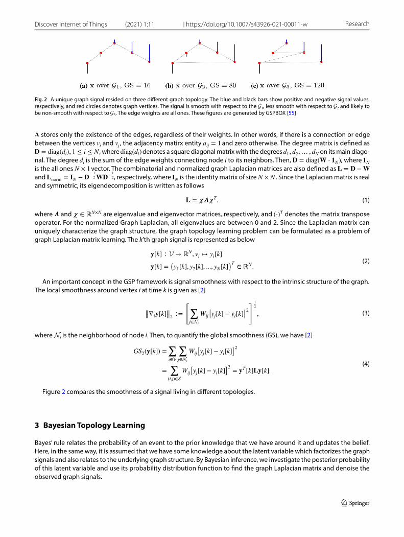
Figure 2 compares the smoothness of a signal living in different topologies.
3 Bayesian Topology Learning
Bayes’ rule relates the probability of an event to the prior knowledge that we have around it and updates the belief. Here, in the same way, it is assumed that we have some knowledge about the latent variable which factorizes the graph signals and also relates to the underlying graph structure. By Bayesian inference, we investigate the posterior probability of this latent variable and use its probability distribution function to find the graph Laplacian matrix and denoise the observed graph signals.
(1)� = ���T ,
(2)�[k] ∶ V → ℝ
N , vi ↦ yi[k]
�[k] =(y1[k], y2[k], ..., yN[k]
)T∈ ℝ
N ,
(3)‖‖∇i�[k]
‖‖2 ∶=
[∑
j∈Ni
Wij
[yj[k] − yi[k]
]2
] 1
2
,
(4)
GS2(�[k]) =∑
i∈V
∑
j∈Ni
Wij
[yj[k] − yi[k]
]2
=∑
(i,j)∈E
Wij
[yj[k] − yi[k]
]2= �T [k]��[k].
Fig. 2 A unique graph signal resided on three different graph topology. The blue and black bars show positive and negative signal values, respectively, and red circles denotes graph vertices. The signal is smooth with respect to the G
1 , less smooth with respect to G
2 and likely to
be non-smooth with respect to G3 . The edge weights are all ones. These figures are generated by GSPBOX [55]
Vol:.(1234567890)
Research Discover Internet of Things (2021) 1:11 | https://doi.org/10.1007/s43926-021-00011-w
1 3
Assume that we are given a data matrix � of size N × K , containing noisy graph signal measurements in its columns. The rows of the matrix � correspond to the vertices of the underlying graph and each column/measurement is as follows
Let us adopt a multi-variate Gaussian distribution for the measurement noise �[k] , given by the following probability density function (pdf )
where � ∈ ℝN is all zero vector.3
To find the underlying graph topology, first, we use the factor analysis model to leverage a representation matrix that can be linked to the graph Laplacian/topology directly. In this model, each graph signal is represented by �[k] = ��[k] + �[k], ∀k , where the unobserved latent variable �[k] ∈ ℝ
N controls each graph signal via the eigenvec-tor matrix � [56] and �[k] ∈ ℝ
N is the mean of graph signal �[k] . For simplicity and without loss of generality, hereafter, it is assumed that ∀k, �[k] = � . As discussed in [53], the motivation of using the factor analysis model is that each graph signal can contribute to the underlying graph structure estimation. Similar to [53], it is assumed that �[k] follows a degenerate zero mean multi-variate Gaussian distribution as follows
where (⋅)† denotes the Moore–Penrose pseudo-inverse and � is the precision matrix. Considering all graph signals, we have
where � = [�[1],… , �[K]] and � = [�[1],… , �[K]] . Equivalently, by using the Kronecker product ⊗ property, all given data can be vectorized as follows
where � = vec(�) , � = �⊗ � , � = vec(�) , � = vec(�) , and vec(⋅ ) stacks all columns of the matrix in a column vector. Thus, we have the following pdf’s
where �0 = �⊗� . By applying the eigenvector matrix identity ��T = � and Kronecker product properties, we have
and thus, the covariance matrix of � in (12) is simplified as follows
where �† = ��†�T.The posterior density of � is obtained by applying the Bayes rule as follows
(5)�[k] = �[k] + �[k], k = 1,…K.
(6)p(�[k];�) ∼ N(�, ��N)
(7)p(�[k];�†
)∼ N(�,�†),
(8)� = �� + �,
(9)� = �� + �,
(10)p(�;�†
)∼ N(�,�
†
0),
(11)p(� ∣ �;� , �) ∼ N(��, ��),
(12)p(�;�†,� , �
)∼ N
(
�,��†
0�T + ��
)
,
(13)��†
0�T = (�⊗ �)
(�⊗�†
)(�⊗ �)T = �⊗ ��†�T ,
(14)��†
0�T + 𝜎� = �⊗
(�† + 𝜎�
),
3 we used � to refer to the noise variance instead of commonly used �2 which is mostly used in the literature. Hereafter, we also remove the subscript notation of �
N , �
N and �
N and assume that the reader infers the corresponding dimensions from the context. The reason is the
notation simplification in the next sections.
Vol.:(0123456789)
Discover Internet of Things (2021) 1:11 | https://doi.org/10.1007/s43926-021-00011-w Research
1 3
and the Minimum Mean Square Error (MMSE) estimator of the latent variable is defined as below [57]
where the covariance matrix is
If � increases, the distributions in (11) and (12) have larger uncertainties and thus the estimation of (16) is less accurate and has a larger MSE. Due to the linear relationship between � and � , i.e. � = �� , the graph signals can be estimated by �̂ = ��� , which can be simplified as follows
where � and � will be estimated later. Equivalently, (18) can be represented in a matrix form as �̂ = (� + 𝜎�)−1� which is similar to the one presented in [53], where �̂ = (� + 𝛼�)−1� for a parameter � . In [53], � is the regularization parameter corresponding to the smoothness of graph signals over the topology. In other words, the graph signals � are smoothed by the graph filter (� + ��)−1 and hence � = � can be called the filter coefficient or the regularization parameter or noise variance, interchangeably. If � approaches zero, �̂ and � are going to be identical and for larger � , the effect of graph Laplacian matrix on filtering the signal is larger. In other words, we have
and thus for the true denoised version of � , i.e. �̂ = � , we have � = 𝜎��̂ . Given a fixed error � , if � is large, then �̂ is suf-ficiently smooth hence ��̂ will likely be small. This is the case where we make a big effort to denoise the observation � . If � is small, the opposite will be true. So this shows that given a noisy observation (hence the amount of noise added to the clean signal is “fixed”), different � estimation approaches (or equivalently � adjustment in [53]) will lead to different denoising effect. However, � has not been investigated analytically in [53] and it was estimated by a grid search.
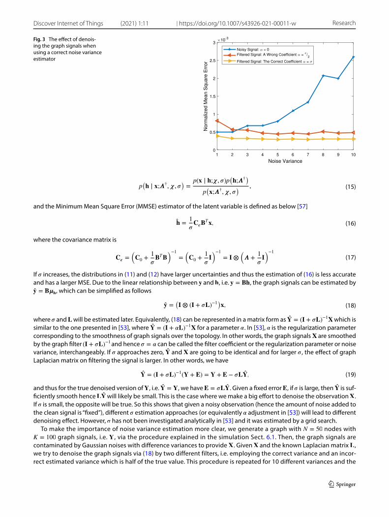
To make the importance of noise variance estimation more clear, we generate a graph with N = 50 nodes with K = 100 graph signals, i.e. � , via the procedure explained in the simulation Sect. 6.1. Then, the graph signals are contaminated by Gaussian noises with difference variances to provide � . Given � and the known Laplacian matrix � , we try to denoise the graph signals via (18) by two different filters, i.e. employing the correct variance and an incor-rect estimated variance which is half of the true value. This procedure is repeated for 10 different variances and the
(15)p(� ∣ �;�†,� , �
)=
p(� ∣ �;� , �)p(�;�†
)
p(�;�†,� , �
) ,
(16)�̂ =1
𝜎���
T�,
(17)�� =
(
�0 +1
𝜎�T�
)−1
=
(
�0 +1
𝜎�)−1
= �⊗(
� +1
𝜎�)−1
(18)�̂ =(�⊗ (� + 𝜎�)−1
)�,
(19)�̂ = (� + 𝜎�)−1(� + �) = � + � − 𝜎��̂,
Fig. 3 The effect of denois-ing the graph signals when using a correct noise variance estimator
Vol:.(1234567890)
Research Discover Internet of Things (2021) 1:11 | https://doi.org/10.1007/s43926-021-00011-w
1 3
normalized mean square error of the true signals and the estimated ones are computed. The results in Fig. 3 show how we can improve our measurements by the filter in (18), especially when we have a better estimation of the noise variance. Since the Laplacian matrix estimation is performed in the next step based on these measurements, using denoised graph signals certainly helps in a better topology estimation.
To estimate the parameters � and �† , an expectation maximization procedure is used which proceeds by optimiz-ing the following log-likelihood function
where �(⋅) denotes the expectation and �̂† , �̂ , and �̂� are the estimators of �† , � , and � . Hereafter, for brevity of notation,
� denotes all the parameters, i.e. � ∶=(�,� ,�†
)= (�,�) . By using (10)–(12) and (17) and some manipulations, (20) is
rewritten as follows (see Appendix 1 for more details)
where � =1
K�̂�̂T is the empirical covariance matrix of the graph signals and the pseudo-determinant | ⋅ | is used due to
the singularity of � and �0 . The pseudo-determinant of a matrix is the product of its non-zero eigenvalues. To find the optimal parameters, Q must be optimized with respect to each argument iteratively up to a convergence. By taking the derivative with respect to � , we have
where the optimal � is found by a numerical method, e.g. Newton–Raphson algorithm. Then, Q is maximized with respect to the Laplacian matrix as follows
where the first three constraints ensure a valid Laplacian matrix and the last one avoids trivial solution for c > 0 . The second term of the objective function promotes the signal smoothness over the estimated topology [as explained in (4)]. The optimization problem in (23) is not easy to implement due to the first and third terms. To solve the issue with the pseudo determinant term, we propose the following minimization problem
where det (⋅) stands for the determinant and � =1
N��T . The equivalence of logdet (� + �) and log|�| has been justified
in [24]. The matrix inverse term which needs high computational power can also be replaced by a less computation-ally expensive term. Theorem 1 of [58] proposed upper and lower bounds for the trace of symmetric positive definite matrices inverse as
and thus for a fixed � , minimizing �‖�‖2F
results in the minimization of Tr((�� + �)−1
) . To sum up, we propose to solve
the following minimization problem for the Laplacian matrix estimation
(20)Q(�†,� , 𝜎
)= �
�∣�;�̂�,�̂ ,�̂†
[log p
(�, � ∣ 𝜎,� ,�†
)],
(21)Q(�) =��∣�;�̂
[log p(� ∣ �)
]+ ��∣�;�̂
[log p(�)
]
∝ − N log 𝜎 − Tr((𝜎� + �)−1
)+ log |�| − Tr(��),
(22)−N
�+ Tr
((�� + �)−1 ⋅ � ⋅ (�� + �)−1
)= 0,
(23)argmax
�
log |�| − Tr(��) − Tr((�� + �)−1
)
s.t. �ij = �ji, �ij ≤ 0 if i ≠ j, � ⋅ � = �, Tr(�) = c,
(24)argmin
�
− logdet (� + �) + Tr(��) + Tr((�� + �)−1
)
s.t. �ij = �ji, �ij ≤ 0 if i ≠ j, � ⋅ � = �, Tr(�) = c,
(25)Tr�(�� + �)−1
�≤ N −
c2�
�‖�‖2F− c
,
(26)Tr�(�� + �)−1
�≥
N
2� + 1−
c2�−2cN�+2N2�
2�+1
�‖�‖2F− c − 2N − 2c�
Vol.:(0123456789)
Discover Internet of Things (2021) 1:11 | https://doi.org/10.1007/s43926-021-00011-w Research
1 3
where ‖�‖2F
can also be considered as the control term for the distribution of off-diagonal elements, i.e. the edge weights of the estimated graph. Since (27) is a convex optimization problem, any off the shelf convex solver may be used, e.g. YALMIP [59]. However, in the next section, a proximal point algorithm is proposed to solve (27) efficiently. To conclude this section, the three steps of the proposed method are presented in Algorithm 1.
4 The efficient implementation
In this section, we discuss milestones to implement the proposed method with a fast and efficient algorithm. The proposed algorithm to solve (27) follows these steps: first by Proposition 2, the last three constraints in (27) are rewrit-ten in the form of inner product of two matrices, helping to form a simpler Lagrangian function. Then, the Lagrangian is iteratively maximized with respect to the dual variable and then minimized with respect to the primal variable, i.e. the graph Laplacian matrix. To do the minimization step, we apply a proximal point algorithm. The maximization can be done by the Newton or quasi-Newton methods where the derivative and Hessian with respect to the dual variable are obtained by Lemma 2 and 1. Theorem 1 finds the stopping criterion guaranteeing the convergence of iteration between the maximization and minimization problem.
Proposition 1 Since � is a symmetric matrix, the summation over all entries of the i’th row (or i’th column) is rewritten as
where �i is an N × N matrix in which the i’th column is the all one vector and the rest is zero.
Proposition 2 Having, � ⋅ � = � , the constraint �ij ≤ 0 for i ≠ j in the problem (27) can be replaced by ‖�‖1 = 2Tr(�) , where ‖�‖1 =
∑i,j abs(Lij) and � ∈ SN
+.
Proof The weight matrix � is a matrix with zero diagonal entries as long as we have assumed that there is no self loop. If all edges are positive (and so �ij ≤ 0 for i ≠ j ), we have ‖�‖1 = ‖�‖1 and
If there is only one edge with negative weight (or correspondingly ∃i ≠ j , �ij > 0 ), ‖�‖1 ≠ ‖�‖1.Note that if all edges are negative and thus �ij ≥ 0 and �ii ≤ 0 , this property is proved in the same way. However, this
is not the case here as long as it is assumed that � ∈ SN+
, forcing the diagonal entries of � to be non-negative. ◻
By applying the Propositions 1 and 2, the minimization problem of (27) is rewritten in the following form
(27)argmin
�
− logdet (� + �) + Tr(��) + �‖�‖2F
s.t. �ij = �ji, �ij ≤ 0 if i ≠ j, � ⋅ � = �, Tr(�) = c,
(28)N∑
j=1
Lij =1
2Tr(�(�i + �T
i
))
(29)‖�‖1 = ‖� −�‖1 = ‖�‖1 + ‖�‖1 = 2‖�‖1 = 2Tr(�) = 2Tr(�).
Vol:.(1234567890)
Research Discover Internet of Things (2021) 1:11 | https://doi.org/10.1007/s43926-021-00011-w
1 3
where � = [�; c; 2c]T , and B(⋅) ∶ RN×N→ R(N+2)×1 is a matrix operator as follows
Hereafter, we interchangeably use the inner product of two matrices instead of the trace operator, i.e. Tr(�1 ⋅ �2) = ⟨�1,�2⟩ . It is assumed that the feasible set F = {� ∈ SN
+, B(�) = �} is not empty and then due to the
convexity of (30), any local optimal solution is also global optimal. The Lagrangian function over the primal variable � and the dual variable � = [�1,… , �N , �N+1, �N+2] is given as below
Since the objective function of (30) is convex and there exists a strictly feasible point (in F ), Slater’s condition holds and there is a strong duality or saddle point property [60]. Strong duality means that it is possible to find the optimal of the dual problem instead of the primal one. Thus, � can be estimated via the following optimization problem
where
However, it is difficult to implement (33) directly. Therefore, we propose to use the proximal algorithm, which is an standard tool for solving constrained and nonsmooth minimization problems [61]. The proximal operator of a closed proper convex function g ∶ Rn
→ R ∪ {+∞} is represented by ����g ∶ Rn→ Rn and its scaled version with parameter
� is given as below
One of the tools for solving the general optimization problem �̂ = argmin�
g(�) is the proximal point algorithm, also
called proximal iteration, given by
where t is the iteration index. In this algorithm, �k and g(�k) converge to the set of minimizers of g and its optimal value,
respectively [62]. The proximal operator provides a smoothed version of the function by adding the regularized term. The proximal operator can also be computed by [61]
where ∇ is the gradient operator and M�g(�) is the Moreau–Yosida regularization. The Moreau–Yosida regularization of g(�) in (33) with parameter 𝜂 > 0 is defined as [61, 63, 64]
where (a)= follows from Von Neumann–Fan minimax theorem [65, 66]. Like the proximal operator, the Moreau-Yosida regularization provides a smooth version of the function. Moreover, M�g(�) and g(�) have the same set of minimizers
(30)argmin�∈SN
+
− logdet (� + �) + Tr(��) + �‖�‖2F
s.t. B(�) = �,
(31)B(�) =�1
2Tr����1 + �T
1
��,… ,
1
2Tr����N + �T
N
��, Tr(�), ‖�‖1
�T,
(32)L(�;�) = −logdet (� + �) + Tr(��) + �‖�‖2F+ �T (� − B(�)),
(33)�̂ = argmin�∈SN
+
g(�),
(34)g(�) = max�
L(�;�).
(35)�����g(�) = argmin�
�
g(�) +1
2�‖� − �‖2
2
�
.
(36)�(t+1) ∶= �����g(�(t)
)
(37)�����g(�) = � − �∇M�g(�),
(38)
M�g(�) = min��∈SN+
{
g(��)+
1
2�‖‖� − ��‖
‖2
F
}
(a)=max
�min��∈SN+
{
L(��;�
)+
1
2�‖‖� − ��‖
‖2
F
}
Vol.:(0123456789)
Discover Internet of Things (2021) 1:11 | https://doi.org/10.1007/s43926-021-00011-w Research
1 3
and thus we solve (38) instead of (34), equivalently. In particular, we propose to find the minimum of M�g(�) by applying the proximal point algorithm in (36).
4.1 Finding ��
(�;�
)
The adjoint operator of B , called hereafter Ba , is obtained as follows
where ���
denotes the partial derivative with respect to � and (a) follows the inner product property. By using (31) and some simple manipulations, we have
To simplify (38), we introduce the change of variable �� as
and then ��(�;�) can be rewritten as follows
where
To find the minimizer of J�
(�′,�;�
) and simplify (42), the following Lemma from [67] will be used.
Lemma 1 [67]: Let � ∈ SN with eigenvalue decomposition � = ���T and 𝛾 > 0 where � = diag(�) is the eigenvalue matrix. Assume two scalar functions �+
�(x) ≜ 1
2
�√x2 + 4� + x
�
and �−�(x) ≜ 1
2
�√x2 + 4� − x
�
are defined and their matrix counter-
parts are as follows
Then,
1. � = �1 − �2 and �1�2 = ��
2. �+�
is continuously differentiable and its derivative at � for every � ∈ SN is given as
where ◦ denotes the Hadamard product and � ∈ SN is defined as follows
(39)Ba(�) =�⟨�,Ba(�)⟩
��
(a)=
�⟨B(�), �⟩
��,
(40)Ba(�) =1
2�1(�1 + �T
1
)+⋯ +
1
2�N
(�N + �T
N
)+ �N+1� + �N+2(2� − N�).
(41)��(�;�) ≜1
1 + 2��
(� − �
(� − Ba(�)
)),
(42)��(�;�) = �T� +1
2�‖�‖2
F−
1 + 2��
2�
�����(�;�)
���
2
F+min
��J�
���,�;�
�
(43)J�
(��,�;�
)= −logdet (��) +
1 + 2��
2�
‖‖‖�� − ��(�;�)
‖‖‖
2
F.
(44)�1 = �+
�(�) = �diag(�+
�(�))�T
�2 = �−�(�) = �diag(�−
�(�))�T
(45)��+
�
�x
|||||x=�
⋅ [�] = �(�◦(�T��)
)�T ,
(46)𝛺ij =𝜙+𝛾(𝜃i) + 𝜙+
𝛾(𝜃j)
√
𝜃2i+ 4𝛾 +
√𝜃2j+ 4𝛾
, 1 < i, j < N.
Vol:.(1234567890)
Research Discover Internet of Things (2021) 1:11 | https://doi.org/10.1007/s43926-021-00011-w
1 3
3.
Proof See [67]. ◻
To find the minimizer of J�
(�′,�;�
) , the derivative with respect to �′ is set to zero as follows
and by some simple manipulations, the solution is �� = �+� �
(��(�;�)
) where � � = �
1+2�� . Then (42) is simplified as follows
(see Appendix 2)
4.2 Find M�g(�) via (38)
Lemma 2 The derivative of ��(�;�) with respect to � is
where �+ ∶= �+� �
(��(�;�)
).
Proof See Appendix 3. ◻
By taking the derivative of ∇���(�;�) with respect to � and applying (45), the following corollary follows.
Corollary 1 The Hessian of ��(�;�) with respect to � is
Using the first and second order derivatives of ��(�;�) with respect to � , the unconstrained maximization problem of (38) can be solved by Newton or quasi-Newton methods, like L-BFGS. Let �opt denote argmax
�
��(�;�) and by using (38),
we have M�g(�) = ��
(�;�opt
).
Lemma 3 The derivative of M�g(�) with respect to the graph Laplacian matrix is
Proof The result follows by taking the derivative of (49) with respect to � and applying Lemma 1, part (3), similar to the proof of Lemma 2. ◻
Considering (36), (37), and (52), the graph Laplacian matrix is estimated via the following iteration rule
(47)��+
�
�x
|||||x=�
⋅ [�1 + �2] = �+�(�).
(48)−(��)−1
+1 + 2��
�
(�� − ��(�;�)
)
(49)��(�;�) = �T� +1
2�‖�‖2
F− logdet
�
�+� �
���(�;�)
��
−1
2� �����+� �
���(�;�)
����
2
F+ N.
(50)∇���(�;�) = � − B(�+
),
(51)∇2
���� = −� �[B
((�+
)�⋅ [1
2
(�1 + �T
1
)]
)
,… ,B((
�+)�⋅ [1
2
(�N + �T
N
)]
)
,
B((
�+)�⋅ [�]
)
,B((
�+)�⋅ [2� − ��T ]
)
],
(52)∇M�g(�) =1
�
(
� − �+� �
(��(�;�opt)
))
.
(53)�(t+1) = �+� �
(
��(�(t);�
(t+1)
opt )
)
.
Vol.:(0123456789)
Discover Internet of Things (2021) 1:11 | https://doi.org/10.1007/s43926-021-00011-w Research
1 3
where (t) stands for the iteration index. All steps to update the Laplacian matrix are summarized in Algorithm 2. It is also possible to use �t rather than � to show the possibility of adjustment in each iteration for a faster convergence of the objective variable � . To find �t in each iteration, the exact or backtracking line search can be applied [60, 61].
5 Convergence analysis
Assume that the eigendecomposition of ��(�;�) is represented as �� = ���T . Hence, we have
where the scalar function �+�(⋅) is a convex function and also bounded with bounded eigenvalues. From theorems B and
C in [68], it follows that �+�(�) is Lipschitz continuous. Thus,
where lc is the Lipschitz constant and �(t)�
= ��
(
�(t);�(t)
opt
)
.
Lemma 4 The scalar function �+�(x) is Lipschitz continuous with the Lipschitz constant 3
2.
Proof See Appendix 4. ◻
Lemma 5 If � is a real symmetric matrix with the eigenvalue matrix �Z , then ‖�‖2F= ���Z
��2
F.
Proof See Appendix 5. ◻
Corollary 2 The matrix valued function �+�(�) is Lipschitz continuous with the constant lc =
9
4.
Proof The proof follows readily by applying the eigenvalue decomposition (44) and using Lemma 4 and 5. ◻
Theorem 1 The proposed BTL-PPA converges when the following stopping criterion is set for dual variables update
where the optimum primal and dual variables are �(t∗) and �(t∗) , respectively.
Proof See Appendix 6. ◻
(54)�+�(��) = �diag(�+
�(�))�T .
(55)‖‖‖‖�+� �
(
�(t)�
)
− �+� �
(
�(t−1)�
)‖‖‖‖
2
F
≤ lc‖‖‖�(t)�− �(t−1)
�
‖‖‖
2
F,
(56)‖‖‖�(t) − �(t∗)‖‖
‖
2
2≤
1
�2N2
‖‖‖�(t) − �(t∗)‖‖
‖
2
F,
Vol:.(1234567890)
Research Discover Internet of Things (2021) 1:11 | https://doi.org/10.1007/s43926-021-00011-w
1 3
6 Numerical results
The proposed algorithm is tested for simulated and real data for different scenarios. For topology learning performance, the results of our algorithm are compared to those of three existing algorithms: GL-SigRep [53], CGL [24], and the learn-ing sparse graph algorithm in [22], called LSG here. In synthetic data simulation part, although the performance of the LSG algorithm is similar to the BTL-PPA, it has a higher computational complexity compared to the other three algorithms. The results for signal recovery performance are only compared to those of GL-SigRep, because the other two methods have no policy for signal representation and recovery. To implement GL-SigRep, an optimal selection of the regularization parameters via exhaustive search is applied and thus the appropriate �
� ratio is found in order to maximize the perfor-
mance for the algorithm in [53].
6.1 Synthetic data
The synthetic data is drawn from a Gaussian Markov Random Field process. First, an Erdős–Rényi graph is generated with N = 40 vertices and an edge probability of 0.2. The weight matrix and then the graph Laplacian matrix are computed and normalized by its trace. Then, each data vector is sampled from a N-variate Gaussian distribution �[k] ∼ N(�,�†) and contaminated by independent and identically distributed Gaussian noise. The measurements are �[k] = �[k] + �[k] for k = 1,… , 4000 and different value of noise variance � . The measurements are stacked in the columns of the matrix � , which is the given input to Algorithm 1. We set c = N [53] and initialize � to 1. Finally, the simulation results are averaged over 100 different trials of experiments.
The most important performance measures to compare different algorithms in this literature are as follows [53, 69–72]:
• Normalized Mean Squared Deviation of graph topology estimation: NMSD =1
N2⋅
‖�−�̂‖2
F
‖�‖2F
, where �̂ denotes the esti-
mated Laplacian matrix,
• Normalized Mean Squared Error of signal reconstruction: NMSE =1
N⋅K⋅
‖�−�̂‖2
F
‖�‖2F
,
• F-measure =2⋅Precision⋅Recall
Precision+Recall=
2TP
2TP+FN+FP , where TP, FP and FN are the numbers of true positives, false positives, and
false negatives, respectively. Also, precision is the number of correctly recovered edges to the number of reconstructed edges in the estimated graph and recall is the number of correctly recovered edges to the number of edges in the ground-truth graph. This performance measure solely takes into account the support of the recovered graph while ignoring the weights,
• Normalized Mutual Information: NMI(�, �̂) =2MI(�,�̂)
H(�)+H(�̂) , where MI is the mutual information between the set of edges
in the estimated graph and the true graph and H(�) is the entropy based on the probability distribution of edges, i.e. the probability of zeros and ones in the matrix � [72].
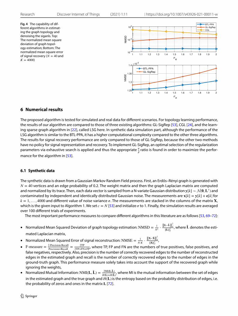
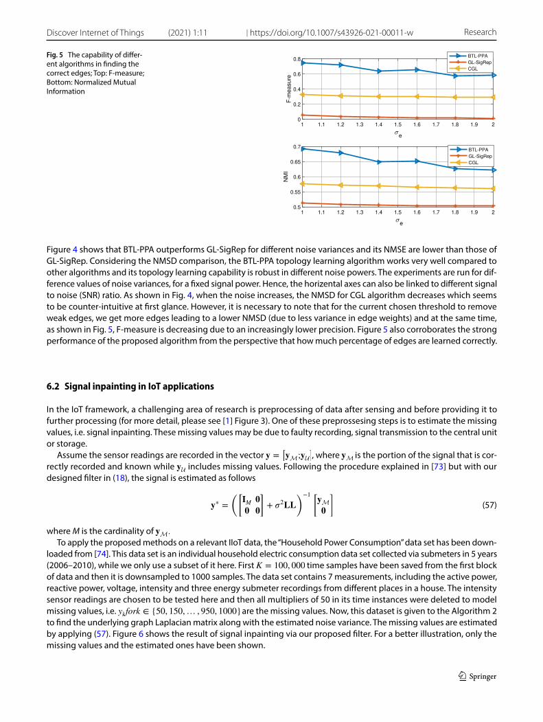
Fig. 4 The capability of dif-ferent algorithms in estimat-ing the graph topology and denoising the siganls. Top: The normalized mean square deviation of graph topol-ogy estimation; Bottom: The normalized mean square error of signal recovery ( N = 40 and K = 4000)
Vol.:(0123456789)
Discover Internet of Things (2021) 1:11 | https://doi.org/10.1007/s43926-021-00011-w Research
1 3
Figure 4 shows that BTL-PPA outperforms GL-SigRep for different noise variances and its NMSE are lower than those of GL-SigRep. Considering the NMSD comparison, the BTL-PPA topology learning algorithm works very well compared to other algorithms and its topology learning capability is robust in different noise powers. The experiments are run for dif-ference values of noise variances, for a fixed signal power. Hence, the horizental axes can also be linked to different signal to noise (SNR) ratio. As shown in Fig. 4, when the noise increases, the NMSD for CGL algorithm decreases which seems to be counter-intuitive at first glance. However, it is necessary to note that for the current chosen threshold to remove weak edges, we get more edges leading to a lower NMSD (due to less variance in edge weights) and at the same time, as shown in Fig. 5, F-measure is decreasing due to an increasingly lower precision. Figure 5 also corroborates the strong performance of the proposed algorithm from the perspective that how much percentage of edges are learned correctly.
6.2 Signal inpainting in IoT applications
In the IoT framework, a challenging area of research is preprocessing of data after sensing and before providing it to further processing (for more detail, please see [1] Figure 3). One of these preprossesing steps is to estimate the missing values, i.e. signal inpainting. These missing values may be due to faulty recording, signal transmission to the central unit or storage.
Assume the sensor readings are recorded in the vector � =[�M;�U
] , where �M is the portion of the signal that is cor-
rectly recorded and known while �U includes missing values. Following the procedure explained in [73] but with our designed filter in (18), the signal is estimated as follows
where M is the cardinality of �M.
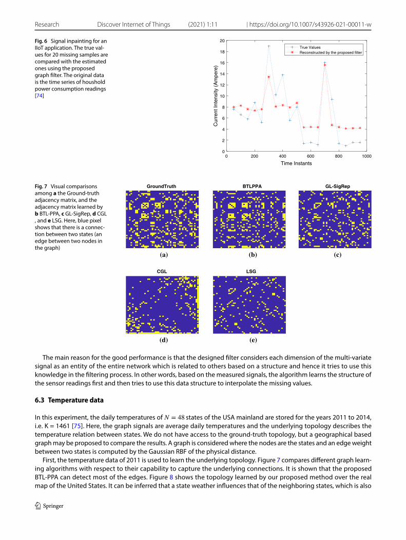
To apply the proposed methods on a relevant IIoT data, the “Household Power Consumption” data set has been down-loaded from [74]. This data set is an individual household electric consumption data set collected via submeters in 5 years (2006–2010), while we only use a subset of it here. First K = 100, 000 time samples have been saved from the first block of data and then it is downsampled to 1000 samples. The data set contains 7 measurements, including the active power, reactive power, voltage, intensity and three energy submeter recordings from different places in a house. The intensity sensor readings are chosen to be tested here and then all multipliers of 50 in its time instances were deleted to model missing values, i.e. ykfork ∈ {50, 150,… , 950, 1000} are the missing values. Now, this dataset is given to the Algorithm 2 to find the underlying graph Laplacian matrix along with the estimated noise variance. The missing values are estimated by applying (57). Figure 6 shows the result of signal inpainting via our proposed filter. For a better illustration, only the missing values and the estimated ones have been shown.
(57)�∗ =
([�M �
� �
]
+ �2��
)−1 [�M�
]
Fig. 5 The capability of differ-ent algorithms in finding the correct edges; Top: F-measure; Bottom: Normalized Mutual Information
Vol:.(1234567890)
Research Discover Internet of Things (2021) 1:11 | https://doi.org/10.1007/s43926-021-00011-w
1 3
The main reason for the good performance is that the designed filter considers each dimension of the multi-variate signal as an entity of the entire network which is related to others based on a structure and hence it tries to use this knowledge in the filtering process. In other words, based on the measured signals, the algorithm learns the structure of the sensor readings first and then tries to use this data structure to interpolate the missing values.
6.3 Temperature data
In this experiment, the daily temperatures of N = 48 states of the USA mainland are stored for the years 2011 to 2014, i.e. K = 1461 [75]. Here, the graph signals are average daily temperatures and the underlying topology describes the temperature relation between states. We do not have access to the ground-truth topology, but a geographical based graph may be proposed to compare the results. A graph is considered where the nodes are the states and an edge weight between two states is computed by the Gaussian RBF of the physical distance.
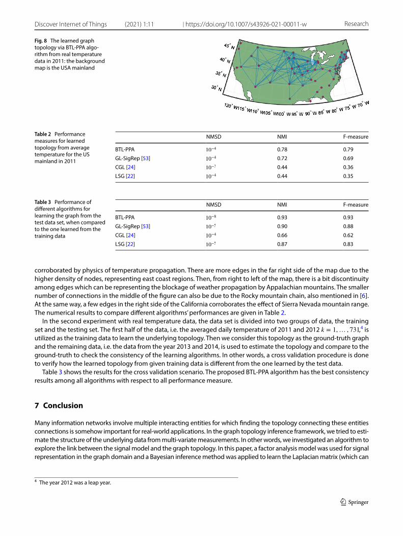
First, the temperature data of 2011 is used to learn the underlying topology. Figure 7 compares different graph learn-ing algorithms with respect to their capability to capture the underlying connections. It is shown that the proposed BTL-PPA can detect most of the edges. Figure 8 shows the topology learned by our proposed method over the real map of the United States. It can be inferred that a state weather influences that of the neighboring states, which is also
Fig. 6 Signal inpainting for an IIoT application. The true val-ues for 20 missing samples are compared with the estimated ones using the proposed graph filter. The original data is the time series of houshold power consumption readings [74]
0 200 400 600 800 1000
Time Instants
0
2
4
6
8
10
12
14
16
18
20
Cur
rent
Inte
nsity
(A
mpe
re)
True ValuesReconstructed by the proposed filter
Fig. 7 Visual comparisons among a the Ground-truth adjacency matrix, and the adjacency matrix learned by b BTL-PPA, c GL-SigRep, d CGL , and e LSG. Here, blue pixel shows that there is a connec-tion between two states (an edge between two nodes in the graph)
GroundTruth
(a)
BTLPPA
(b)
GL-SigRep
(c)
CGL
(d)
LSG
(e)
Vol.:(0123456789)
Discover Internet of Things (2021) 1:11 | https://doi.org/10.1007/s43926-021-00011-w Research
1 3
corroborated by physics of temperature propagation. There are more edges in the far right side of the map due to the higher density of nodes, representing east coast regions. Then, from right to left of the map, there is a bit discontinuity among edges which can be representing the blockage of weather propagation by Appalachian mountains. The smaller number of connections in the middle of the figure can also be due to the Rocky mountain chain, also mentioned in [6]. At the same way, a few edges in the right side of the California corroborates the effect of Sierra Nevada mountain range. The numerical results to compare different algorithms’ performances are given in Table 2.
In the second experiment with real temperature data, the data set is divided into two groups of data, the training set and the testing set. The first half of the data, i.e. the averaged daily temperature of 2011 and 2012 k = 1,… , 731,4 is utilized as the training data to learn the underlying topology. Then we consider this topology as the ground-truth graph and the remaining data, i.e. the data from the year 2013 and 2014, is used to estimate the topology and compare to the ground-truth to check the consistency of the learning algorithms. In other words, a cross validation procedure is done to verify how the learned topology from given training data is different from the one learned by the test data.
Table 3 shows the results for the cross validation scenario. The proposed BTL-PPA algorithm has the best consistency results among all algorithms with respect to all performance measure.
7 Conclusion
Many information networks involve multiple interacting entities for which finding the topology connecting these entities connections is somehow important for real-world applications. In the graph topology inference framework, we tried to esti-mate the structure of the underlying data from multi-variate measurements. In other words, we investigated an algorithm to explore the link between the signal model and the graph topology. In this paper, a factor analysis model was used for signal representation in the graph domain and a Bayesian inference method was applied to learn the Laplacian matrix (which can
Fig. 8 The learned graph topology via BTL-PPA algo-rithm from real temperature data in 2011: the background map is the USA mainland
Table 2 Performance measures for learned topology from average temperature for the US mainland in 2011
NMSD NMI F-measure
BTL-PPA 10−4 0.78 0.79
GL-SigRep [53] 10−4 0.72 0.69
CGL [24] 10−3 0.44 0.36
LSG [22] 10−4 0.44 0.35
Table 3 Performance of different algorithms for learning the graph from the test data set, when compared to the one learned from the training data
NMSD NMI F-measure
BTL-PPA 10−8 0.93 0.93
GL-SigRep [53] 10−5 0.90 0.88
CGL [24] 10−4 0.66 0.62
LSG [22] 10−5 0.87 0.83
4 The year 2012 was a leap year.
Vol:.(1234567890)
Research Discover Internet of Things (2021) 1:11 | https://doi.org/10.1007/s43926-021-00011-w
1 3
uniquely represent the graph topology) and to estimate the noise variance at the same time. To formulate the problem, we used a Bayesian framework and proposed a minimum mean square estimation approach to denoise the measurements. Finally, a convex optimization problem over the graph Laplacian matrix was proposed and solved via a proximal point method to estimate the topology from a denoised version of graph signals. The experimental results corroborate the performance of the proposed algorithm for a wide range of sensor networks and IoT applications.
Acknowledgements This material is based upon work partially supported by the U. S. Army Research Laboratory and the U. S. Army Research Office under grant number W911NF-17-1-0331 and by the National Science Foundation under grants ECCS-1744129, CNS-1702555, DMS-1736417 and ECCS-1824710.
Authors’ contributions MRM: proposed the main idea of the paper, worked on analytical perspective and computations, derived the both algorithms in the paper, collected the data and had done simulations. MH: helped in writing and edited the paper. KS: Helped partially in some maths of the paper. XD: Helped in the main idea and adding the first three figures. RSB: was the main reviewer and editor of the paper. HVP: reviewed the paper and gave general comments. All authors reviewed the manuscript. All authors read and approved the final manuscript.
Declarations
Competing interests The authors declare no competing interests.
Open Access This article is licensed under a Creative Commons Attribution 4.0 International License, which permits use, sharing, adapta-tion, distribution and reproduction in any medium or format, as long as you give appropriate credit to the original author(s) and the source, provide a link to the Creative Commons licence, and indicate if changes were made. The images or other third party material in this article are included in the article’s Creative Commons licence, unless indicated otherwise in a credit line to the material. If material is not included in the article’s Creative Commons licence and your intended use is not permitted by statutory regulation or exceeds the permitted use, you will need to obtain permission directly from the copyright holder. To view a copy of this licence, visit http:// creat iveco mmons. org/ licen ses/ by/4. 0/.
Appendices
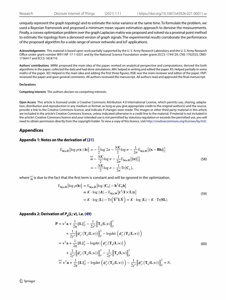
Appendix 1: Notes on the derivation of (21)
where (a)∝ is due to the fact that the first term is constant and will be ignored in the optimization.
Appendix 2: Derivation of Pη(L; ν), i.e. (49)
(58)
��∣�;�̂
�log p(� ∣ �)
�= −
1
2log 2𝜋 −
NK
2log 𝜎 −
1
2𝜎��∣�;�̂
�‖� − ��‖2
2
�
(a)∝ −
NK
2log 𝜎 −
1
2𝜎��∣�;�̂
�‖�‖2
2
�
= −NK
2log 𝜎 −
1
2𝜎Tr���
�,
(59)
��∣�;�̂
[log p(�)
]= ��∣�;�̂
[log |�0| − �T�0�
]
∝ K ⋅ log |�| − ��∣�;�̂
[�T (� × �)�
]
= K ⋅ log |�| − Tr(
�̂T��̂)
= K ⋅ log |�| − K ⋅ Tr(��).
(60)
� = �T� +1
2�‖�‖2
F−
1
2� ������(�;�)
���
2
F
+1
2� �����−� �
���(�;�)
����
2
F− logdet
�
�+� �
���(�;�)
��
= �T� +1
2�‖�‖2
F− logdet
�
�+� �
���(�;�)
��
+1
2� �����−� �
���(�;�)
����
2
F−
1
2� ������(�;�)
���
2
F
(a)= �T� +
1
2�‖�‖2
F− logdet
�
�+� �
���(�;�)
��
−1
2� �����+� �
���(�;�)
����
2
F+ N,
Vol.:(0123456789)
Discover Internet of Things (2021) 1:11 | https://doi.org/10.1007/s43926-021-00011-w Research
1 3
where (a)= follows from Lemma 1.
Appendix 3: Proof of Lemma 2
To simplify the notation, we define �+ ∶= �+� �
(��(�;�)
) , �− ∶= �−
� �
(��(�;�)
) and
(�+
)�∶=
��+
��
���
;
where the last equality follows from Lemma 1, part (3).
Appendix 4: Proof of Lemma 4
Since the domain of �+�(x) is R , the function is differentiable everywhere, and the derivative is bounded. Thus the Lip-
schitz constant is
where x ∈ ℝ and for all 𝛾 > 0.
Appendix 5: Proof of Lemma 5
We know that when �ii is an eigenvalue of the matrix � , �2ii will be an eigenvalue of �2 . Thus,
Appendix 6: Proof of Theorem 1
To find the optimum dual variable in the second step of the Algorithm 2, if we set the stopping criterion as (56), then (64) can be simplified to
where 2lc
(1+2𝜂𝜎)2< 1 is required for the convergence of � which can be guaranteed by using Corollary 2 and setting � ≥ 3
√2−2
4�
.
References
1. Li S, Da Xu L, Zhao S. The internet of things: a survey. Inf Syst Front. 2015;17(2):243.
(61)∇���(�;�) = � − B
((�+
)��+
)
− � �B((
�+)�(
�+)−1
)
= � − B((
�+)�[
�+ +�−])
= � − B(�+
),
(62)supx
���+
�(x)
�x� = sup
x
�x
√x2 + 4�
+ 0.5� = 1.5,
(63)‖�‖2F= Tr
���T
�= Tr
��2
�=�
i
��Z2
�
ii=�
i
��Z
�2ii= ���Z
��2
F,
(64)
‖‖‖�(t+1) − �(t∗)‖‖
‖
2
F=‖‖‖‖�+� �
(
�(t)�
)
− �+� �
(
�(t∗)�
)‖‖‖‖
2
F
≤ lc‖‖‖�(t)�− �(t∗)
�
‖‖‖
2
F
=lc
(1 + 2��)2‖‖‖
(�(t) − �(t∗)
)+ � ⋅ Ba
(�(t) − �(t∗)
)‖‖‖
2
F
≤lc
(1 + 2��)2
(‖‖‖�(t) − �(t∗)‖‖
‖
2
F+ �2N2‖‖
‖�(t) − �(t∗)‖‖
‖
2
2
)
,
(65)‖‖‖�(t+1) − �(t∗)‖‖
‖
2
F≤
2lc
(1 + 2��)2‖‖‖�(t) − �(t∗)‖‖
‖
2
F,
Vol:.(1234567890)
Research Discover Internet of Things (2021) 1:11 | https://doi.org/10.1007/s43926-021-00011-w
1 3
2. Shuman DI, Narang SK, Frossard P, Ortega A, Vandergheynst P. The emerging field of signal processing on graphs: extending high-dimensional data analysis to networks and other irregular domains. IEEE Signal Process Mag. 2013;30(3):83. https:// doi. org/ 10. 1109/ MSP. 2012. 22351 92.
3. Ortega A, Frossard P, Kovačević J, Moura JM, Vandergheynst P. Graph signal processing: overview, challenges, and applications. Proc IEEE. 2018;106(5):808.
4. Friston KJ. Functional and effective connectivity in neuroimaging: a synthesis. Human Brain Map. 1994;2(1–2):56. 5. Goebel R, Roebroeck A, Kim DS, Formisano E. Investigating directed cortical interactions in time-resolved fMRI data using vector autore-
gressive modeling and Granger causality mapping. Magn Resonance Imaging. 2003;21(10):1251. 6. Mei J, Moura JM. Signal processing on graphs: causal modeling of unstructured data. IEEE Trans Signal Process. 2017;65(8):2077. 7. Bolstad A, Veen BDV, Nowak R. Causal network inference via group sparse regularization. IEEE Trans Signal Process. 2011;59(6):2628.
https:// doi. org/ 10. 1109/ TSP. 2011. 21295 15. 8. Shen Y, Baingana B, Giannakis GB. Kernel-based structural equation models for topology identification of directed networks. IEEE Trans
Signal Process. 2017;65(10):2503. https:// doi. org/ 10. 1109/ TSP. 2017. 26640 39. 9. Ramezani-Mayiami M. Joint graph learning and signal recovery via kalman filter for multivariate auto-regressive processes. In: Proceed-
ings of the IEEE 26th European signal processing conference (EUSIPCO); 2018. p. 907–11. https:// doi. org/ 10. 23919/ EUSIP CO. 2018. 85533 84
10. Baccalá LA, Sameshima K. Partial directed coherence: a new concept in neural structure determination. Biol Cybern. 2001;84(6):463. 11. Songsiri J, Vandenberghe L. Topology selection in graphical models of autoregressive processes. J Mach Learn Res. 2010;11(Oct):2671. 12. Shen Y, Baingana B, Giannakis GB. Nonlinear structural vector autoregressive models for inferring effective brain network connectivity;
2016. arXiv preprint. arXiv: 1610. 06551. 13. Baingana B, Giannakis GB. Tracking switched dynamic network topologies from information cascades. IEEE Trans Signal Process.
2016;65(4):985. 14. Ramezani-Mayiami M, Beferull-Lozano B. Graph recursive least squares filter for topology inference in causal data processes In: Proceed-
ings of the IEEE 7th international workshop on computational advances in multi-sensor adaptive processing (CAMSAP); 2017. p. 1–5 15. Traganitis PA, Shen Y, Giannakis GB. Network topology inference via elastic net structural equation models In: Proceedings of the IEEE
25th European signal processing conference (EUSIPCO) (IEEE); 2017. p. 146–50. 16. Ramezani-Mayiami M. Joint Topology Learning and graph signal recovery via KALMAN filter in causal data processes. In: Proceedings of
the IEEE 28th international workshop on machine learning for signal processing (MLSP) (IEEE); 2018. p. 1–6. 17. Dempster AP. Covariance selection. Biometrics. 1972;25:157–75. 18. Banerjee O, Ghaoui LE, d’Aspremont A. Model selection through sparse maximum likelihood estimation for multivariate gaussian or
binary data. J Mach Learn Res. 2008;9(Mar):485. 19. Friedman J, Hastie T, Tibshirani R. Sparse inverse covariance estimation with the graphical LASSO. Biostatistics. 2008;9(3):432. 20. Yuan M, Lin Y. Model selection and estimation in the Gaussian graphical model. Biometrika. 2007;94(1):19. 21. Scheinberg K, Rish I. Learning sparse Gaussian Markov networks using a greedy coordinate ascent approach. In: Joint European confer-
ence on machine learning and knowledge discovery in databases. Berlin: Springer; 2010. p. 196–212. 22. Lake B, Tenenbaum J. Discovering structure by learning sparse graph. In: Proceedings of the 32nd annual meeting of the cognitive science
society; 2010. p. 6160–73. 23. Kalofolias V. How to learn a graph from smooth signals. In: Proceedings of the 19th international conference of artificial intelligence and
statistics, AISTATS, Cadiz; 2016. p. 920–9. 24. Egilmez HE, Pavez E, Ortega A. Graph learning from data under Laplacian and structural constraints. IEEE J Selected Topics Signal Process.
2017;11(6):825. 25. Segarra S, Marques AG, Mateos G, Ribeiro A. Network topology inference from spectral templates. IEEE Trans Signal Inf Process Over Netw.
2017;3(3):467. https:// doi. org/ 10. 1109/ TSIPN. 2017. 27310 51. 26. Pasdeloup B, Gripon V, Mercier G, Pastor D, Rabbat MG. Characterization and inference of graph diffusion processes from observations
of stationary signals. IEEE Trans Signal Inf Process Over Netw. 2018;4(3):481. https:// doi. org/ 10. 1109/ TSIPN. 2017. 27429 40. 27. Shafipour R, Segarra S, Marques AG, Mateos G. Network topology inference from non-stationary graph signals In: Proceedings of the IEEE
international conference on acoustics, speech and signal processing (ICASSP). New York: IEEE; 2017. p. 5870–4. 28. Thanou D, Dong X, Kressner D, Frossard P. Learning heat diffusion graphs. IEEE Trans Signal Inf Process Over Netw. 2017;3(3):484. https://
doi. org/ 10. 1109/ TSIPN. 2017. 27311 64. 29. Egilmez HE, Pavez E, Ortega A. Graph learning from filtered signals: Graph system and diffusion kernel identification. IEEE Trans Signal
Inf Process Over Netw. 2018;5(2):360–74. 30. Ma H, Yang H, Lyu MR, King I. Mining social networks using heat diffusion processes for marketing candidates selection In: Proceedings
of the 17th ACM conference on Information and knowledge management (ACM); 2008. p. 233–42. 31. Yankelevsky Y, Elad M. Dual graph regularized dictionary learning. IEEE Trans Signal Inf Process Over Netw. 2016;2(4):611. 32. Ramezani-Mayiami M, Skretting K. Topology inference and signal representation using dictionary learning In: Proceedings of the IEEE
27th European signal processing conference (EUSIPCO); 2019. 33. Sardellitti S, Barbarossa S, Di Lorenzo P. Graph topology inference based on sparsifying transform learning. IEEE Trans Signal Process.
2019;67(7):1712. 34. Giannakis GB, Shen Y, Karanikolas GV. Topology identification and learning over graphs: accounting for nonlinearities and dynamics. Proc
IEEE. 2018;106(5):787. 35. Varma R, Chen S, Kovačević J. Graph topology recovery for regular and irregular graphs. In: 2017 IEEE 7th international workshop on
computational advances in multi-sensor adaptive processing (CAMSAP). 2017. p. 1–5. https:// doi. org/ 10. 1109/ CAMSAP. 2017. 83132 02. 36. Marinakis D, Dudek G. A practical algorithm for network topology inference. In: Proceedings of the IEEE International Conference on
Robotics and Automation, 2006. ICRA 2006. New York: IEEE. 2006. p. 3108–15. 37. Pavez E, Egilmez HE, Ortega A. Learning graphs with monotone topology properties and multiple connected components. IEEE Trans
Signal Process. 2018;66(9):2399.
Vol.:(0123456789)
Discover Internet of Things (2021) 1:11 | https://doi.org/10.1007/s43926-021-00011-w Research
1 3
38. Satya JP, Bhatt N, Pasumarthy R, Rajeswaran A. Identifying topology of power distribution networks based on smart meter data; 2016. arXiv preprint. arXiv: 1609. 02678.
39. Pavez E, Ortega A. Generalized Laplacian precision matrix estimation for graph signal processing In: Proceedings of the IEEE international conference on acoustics, speech and signal processing (ICASSP). New York: IEEE. 2016. p. 6350–4.
40. Kalofolias V, Loukas A, Thanou D, Frossard P. Learning time varying graphs. In: 2017 IEEE international conference on acoustics, speech and signal processing (ICASSP). New York: IEEE. 2017. p. 2826–30.
41. Dong X, Thanou D, Rabbat M, Frossard P. Learning graphs from data: a signal representation perspective. IEEE Signal Process Mag. 2019;36(3):44. https:// doi. org/ 10. 1109/ MSP. 2018. 28872 84.
42. Mateos G, Segarra S, Marques AG, Ribeiro A. Connecting the dots: identifying network structure via graph signal processing. IEEE Signal Process Mag. 2019;36(3):16. https:// doi. org/ 10. 1109/ MSP. 2018. 28901 43.
43. Kumar S, Ying J, de Miranda Cardoso JV, Palomar D. Structured graph learning via laplacian spectral constraints. In: Advances in neural information processing systems. 2019. p. 11651–63.
44. Wentzell PD. Measurement errors in multivariate chemical data. J Braz Chem Soc. 2014;25(2):183. 45. Azadkia M. Adaptive estimation of noise variance and matrix estimation via usvt algorithm. 2018. arXiv preprint. arXiv: 1801. 10015 46. Zhang S, Ding Z, Cui S. Introducing hypergraph signal processing: theoretical foundation and practical applications. IEEE Internet Things
J. 2019;7(1):639. 47. Liu Y, Dillon T, Yu W, Rahayu W, Mostafa F. Noise removal in the presence of significant anomalies for Industrial IoT sensor data in manufactur-
ing. IEEE Internet Things J. 2020;7:7084–96. 48. Ramezani-Mayiami M, Skretting K. Robust Graph Topology Learning and Application in Stock Market Inference In: 2019 IEEE international
conference on signal and image processing applications (ICSIPA). New York: IEEE. 2019. p. 240–4. 49. Black F. Noise. J Fin. 1986;41(3):528. 50. Chen S, Sandryhaila A, Moura JM, Kovacevic J. Signal denoising on graphs via graph filtering. In: 2014 IEEE global conference on signal and
information processing (GlobalSIP). New York: IEEE. 2014. p. 872–6. 51. Galatsanos NP, Katsaggelos AK. Methods for choosing the regularization parameter and estimating the noise variance in image restoration
and their relation. IEEE Trans Image Process. 1992;1(3):322. 52. Chepuri SP, Liu S, Leus G, Hero AO. Learning sparse graphs under smoothness prior. In: Proceedings of the IEEE international conference on
acoustics, speech and signal processing (ICASSP). New York: IEEE. 2017. p. 6508–12. 53. Dong X, Thanou D, Frossard P, Vandergheynst P. Learning Laplacian matrix in smooth graph signal representations. IEEE Trans Signal Process.
2016;64(23):6160. https:// doi. org/ 10. 1109/ TSP. 2016. 26028 09. 54. Ramezani-Mayiami M, Hajimirsadeghi M, Skretting K, Blum RS, Vincent Poor H. Graph topology learning and signal recovery via Bayesian
inference. In: Proceedings of the IEEE data science workshop (DSW). 2019. p. 52–6. https:// doi. org/ 10. 1109/ DSW. 2019. 87556 01. 55. Perraudin N, Paratte J, Shuman D, Martin L, Kalofolias V, Vandergheynst P, Hammond DK. GSPBOX: a toolbox for signal processing on graphs.
ArXiv e-prints 2014. 56. Basilevsky AT. Statistical factor analysis and related methods: theory and applications, vol. 418. Hoboken: John Wiley & Sons; 2009. 57. Kay SM. Fundamentals of statistical signal processing. Prentice: Prentice Hall PTR; 1993. 58. Bai Z, Golub GH. Bounds for the trace of the inverse and the determinant of symmetric positive definite matrices. Ann Numer Math. 1996;4:29. 59. Löfberg J. YALMIP: a toolbox for modeling and optimization in MATLAB. In: Proceedings of the IEEE international conference on robotics
and automation. 2004. p. 284–9. 60. Boyd S, Vandenberghe L. Convex optimization. Cambridge: Cambridge University Press; 2004. 61. Parikh N, Boyd S, et al. Proximal algorithms. Foundations Trends ® Opt. 2014;1(3):127. 62. Bauschke H, Combettes P, Noll D. Joint minimization with alternating Bregman proximity operators. Pacific J Opt. 2006. https:// hal. archi
ves- ouver tes. fr/ hal- 01868 791/. https:// schol ar. google. com/ schol ar? hl= en& as_ sdt=0% 2C5&q= Joint+ minim izati on+ with+ alter nating+ Bregm an+ proxi mity+ opera tors& btnG=
63. Yosida K. Functional analysis. Berlin: Springer; 1964. 64. Moreau JJ. Proximité et dualité dans un espace hilbertien. Bull Soc Math France. 1965;93(2):273. 65. Neumann Jv. Zur Theorie der Gesellschaftsspiele. Mathematische Annalen. 1928;100(1):295. https:// doi. org/ 10. 1007/ BF014 48847. 66. Von Neumann J. Uber ein okonomsiches gleichungssystem und eine verallgemeinering des browerschen fixpunktsatzes. Erge Math
Kolloq. 1937;8:73–83. 67. Wang C, Sun D, Toh KC. Solving log-determinant optimization problems by a Newton-CG primal proximal point algorithm. SIAM J Opt.
2010;20(6):2994. 68. Roberts AW, Varberg DE. Another proof that convex functions are locally Lipschitz. Am Math Monthly. 1974;81(9):1014. 69. Hu C, Cheng L, Sepulcre J, Johnson KA, Fakhri GE, Lu YM, Li Q. A spectral graph regression model for learning brain connectivity of Alz-
heimer’s disease. PLoS ONE. 2015;10(5):e0128136. 70. Cover TM, Thomas JA. Elements of information theory. Hoboken: John Wiley & Sons; 2012. 71. Goutte C, Gaussier E. A probabilistic interpretation of precision, recall and F-score, with implication for evaluation. In: European confer-
ence on information retrieval. Berlin: Springer. 2005. p. 345–59. 72. Manning C, Raghavan P, Schütze H. Introduction to information retrieval. Nat Lang Eng. 2010;16(1):100. 73. Chen S, Sandryhaila A, Lederman G, Wang Z, Moura JM, Rizzo P, Bielak J, Garrett JH, Kovačevic J. Signal inpainting on graphs via total
variation minimization. In: 2014 IEEE international conference on acoustics, speech and signal processing (ICASSP). New York: IEEE. 2014. p. 8267–71.
74. Ortiz J. Household power consumption 2016; Household Power Consumption, Individual household electric power consumption dataset collected via submeters placed in 3 distinct areas of a home, https:// data. world/ datab eats/ house hold- power- consu mption.
75. National climatic data center. ftp:// ftp. ncdc. noaa. gov/ pub/ data/ gsod/
Publisher’s Note Springer Nature remains neutral with regard to jurisdictional claims in published maps and institutional affiliations.