Discrete gradient method: a derivative freemethod for nonsmooth optimization

Adil M. Bagirov1, Bulent Karasozen2, Meral Sezer3

Communicated by F. Giannessi

1Corresponding author, a.bagirov@ballarat.edu.au, Centre for Informatics and Applied Opti-

mization, School of Information Technology and Mathematical Sciences, University of Ballarat,

Victoria 3353, Australia2Department of Mathematics & Institute of Applied Mathematics, Middle East Technical Uni-

versity, Ankara, Turkey3Department of Mathematics, Middle East Technical University, Ankara, Turkey

1

Abstract

In this paper a new derivative-free method is developed for solving un-

constrained nonsmooth optimization problems. This method is based on the

notion of a discrete gradient. It is demonstrated that the discrete gradients

can be used to approximate subgradients of a broad class of nonsmooth func-

tions. It is also shown that the discrete gradients can be applied to find

descent directions of nonsmooth functions. The preliminary results of nu-

merical experiments with unconstrained nonsmooth optimization problems as

well as the comparison of the proposed method with nonsmooth optimization

solver DNLP from CONOPT-GAMS and derivative-free optimization solver

CONDOR are presented.

Keywords: nonsmooth optimization, derivative-free optimization, subdifferential,

discrete gradients.

Mathematical Subject Classification: 65K05, 90C25.

2

1 Introduction

Consider the following nonsmooth unconstrained minimization problem:

minimize f(x) subject to x ∈ IRn (1)

where the objective function f is assumed to be Lipschitz continuous.

Nonsmooth unconstrained optimization problems appear in many applications

and in particular in data mining. Over more than four decades different methods

have been developed to solve problem (1). We mention among them the bundle

method and its different variations (see, for example, [1, 2, 3, 4, 5, 6, 25, 7]), al-

gorithms based on smoothing techniques [8] and the random subgradient sampling

algorithm [9].

In most of these algorithms at each iteration the computation of at least one

subgradient or approximating gradient is required. However, there are many prac-

tical problems where the computation of even one subgradient is a difficult task.

Therefore in such situations derivative free methods seem to be better choice since

they do not use explicit computation of subgradients.

Among derivative free methods, the generalized pattern search methods are well-

suited for nonsmooth optimization [10, 11]. However their convergence are proved

under quite restrictive differentiability assumptions. It was shown in [11] that when

the objective function f is continuously differentiable in IRn then the limit inferior

of the norm of the gradient of the sequence of points generated by the generalized

pattern search algorithm goes to zero. The paper [10] provides convergence analysis

under less restrictive differentiability assumptions. It was shown that if f is strictly

differentiable near the limit of any refining subsequence, the gradient at that point

is zero. However, in many practically important problems this condition is not

satisfied, because in such problems the objective functions are not differentiable at

local minimizers.

In this paper we develop a new derivative free method based on the notion of a

discrete gradient for solving unconstrained nonsmooth optimization problems. First,

we describe an algorithm for the computation of the subgradients of a broad class

3

of non-regular functions. Then we prove that the discrete gradients can be used

to approximate subdifferentials of such functions. We also describe an algorithm

for the computation of the descent directions of nonsmooth functions using discrete

gradients. It is shown that the proposed algorithm converges for a broad class of

nonsmooth functions. Finally, we present the comparison of the proposed algorithm

with one nonsmooth optimization solver, DNLP from GAMS and one derivative-free

solver CONDOR using results of numerical experiments.

The structure of the paper is as follows. Section 2 provides some necessary def-

initions used in the following sections and Section 3 presents problems from data

clustering where the objective functions are non-regular and nonsmooth. An algo-

rithm for approximation of subgradients is described in Section 4. Discrete gradients

and their application for the approximation of subdifferentials are given in Section 5.

In Section 6 we develop an algorithm for the computation of a descent direction and

Section 7 presents the discrete gradient method. Results of numerical experiments

are given in Section 8. Section 9 concludes the paper.

2 Preliminaries

In this section we will give some definitions which are used in the subsequent sections.

2.1 The Clarke subdifferential

Let f be a function defined on IRn. The function f is called locally Lipschitz

continuous if for any bounded subset X ⊂ IRn there exists an L > 0 such that

|f(x)− f(y)| ≤ L‖x− y‖ ∀x, y ∈ X.

We recall that a locally Lipschitz function f is differentiable almost everywhere

and that we can define for it a Clarke subdifferential [12] by

∂f(x) = co{v ∈ IRn : ∃(xk ∈ D(f), xk → x, k → +∞) : v = lim

k→+∞∇f(xk)

},

here D(f) denotes the set where f is differentiable, co denotes the convex hull of

a set. It is shown in [12] that the mapping ∂f(x) is upper semicontinuous and

bounded on bounded sets.

4

The generalized directional derivative of f at x in the direction g is defined as

f 0(x, g) = lim supy→x,α→+0

α−1[f(y + αg)− f(y)].

If the function f is locally Lipschitz continuous then the generalized directional

derivative exists and

f 0(x, g) = max {〈v, g〉 : v ∈ ∂f(x)}

where 〈·, ·〉 stands for an inner product in IRn. f is called a Clarke regular function on

IRn, if it is differentiable with respect to any direction g ∈ IRn and f ′(x, g) = f 0(x, g)

for all x, g ∈ IRn where f ′(x, g) is a derivative of the function f at the point x with

respect to the direction g:

f ′(x, g) = limα→+0

α−1[f(x + αg)− f(x)].

It is clear that directional derivative f ′(x, g) of the Clarke regular function f is upper

semicontinuous with respect to x for all g ∈ IRn.

Let f be a locally Lipschitz continuous function defined on IRn. For point x to

be a minimum point of the function f on IRn, it is necessary that

0 ∈ ∂f(x).

2.2 Semismooth functions and quasidifferentiability

The function f : IRn → IR1 is called semismooth at x ∈ IRn, if it is locally Lipschitz

continuous at x and for every g ∈ IRn, the limit

limg′→g,α→+0

〈v, g〉, v ∈ ∂f(x + αg′)

exists. It should be noted that the class of semismooth functions is fairly wide and

it contains convex, concave, max- and min-type functions [13]. The semismooth

function f is directionally differentiable and

f ′(x, g) = limg′→g,α→+0

〈v, g〉, v ∈ ∂f(x + αg′).

5

Let f be a semismooth function defined on IRn. Consider the following set at a

point x ∈ IRn with respect to a given direction g ∈ Rn, ‖g‖ = 1:

R(x, g) = co{v ∈ IRn : ∃(vk ∈ ∂f(x + λkg), λk → +0, k → +∞) : v = lim

k→+∞vk

}.

It follows from the semismoothness of f that

f ′(x, g) = 〈v, g〉 ∀v ∈ R(x, g)

and for any ε > 0 there exists λ0 > 0 such that

∂f(x + λg) ⊂ R(x, g) + Sε, (2)

for all λ ∈ (0, λ0). Here

Sε = {v ∈ IRn : ‖v‖ < ε}.A function f is called quasidifferentiable at a point x if it is locally Lipschitz

continuous, directionally differentiable at this point and there exist convex, compact

sets ∂f(x) and ∂f(x) such that:

f ′(x, g) = maxu∈∂f(x)

〈u, g〉+ minv∈∂f(x)

〈v, g〉.

The set ∂f(x) is called a subdifferential, the set ∂f(x) is called a superdifferential

and the pair of sets [∂f(x), ∂f(x)] is called a quasidifferential of the function f at a

point x [14].

3 Data clustering as nonsmooth optimization prob-

lem

There are many applications when the objective and/or constraint functions are

not regular functions. We will mention here only one of them, the cluster analysis

problem, which is an important application area in data mining.

Clustering is also known as the unsupervised classification of patterns, deals

with the problems of organization of a collection of patterns into clusters based

6

on similarity. There are many application of clustering in information retrieval,

medicine etc.

In cluster analysis we assume that we have been given a finite set C of points in

the n-dimensional space IRn, that is

C = {c1, . . . , cm}, where ci ∈ IRn, i = 1, . . . , m.

There are different types of clustering such as partition, packing, covering and hi-

erarchical clustering. We consider here partition clustering, that is the distribution

of the points of the set C into a given number q of disjoint subsets Ci, i = 1, . . . , q

with respect to predefined criteria such that:

1) Ci 6= ∅, i = 1, . . . , q;

2) Ci ⋂Cj = ∅, i, j = 1, . . . , q, i 6= j;

3) C =q⋃

i=1Ci.

The sets Ci, i = 1, . . . , q are called clusters. The strict application of these rules

is called hard clustering, unlike fuzzy clustering, where the clusters are allowed to

overlap. We assume that no constraints are imposed on the clusters Ci, i = 1, . . . , q

that is we consider the hard unconstrained clustering problem.

We also assume that each cluster Ci, i = 1, . . . , q can be identified by its center

(or centroid). There are different formulations of the clustering as an optimization

problem. In [15, 16, 17, 18] the cluster analysis problem is reduced to the following

nonsmooth optimization problem

minimize f(x1, . . . , xq) subject to (x1, . . . , xq) ∈ IRn×q, (3)

where

f(x1, . . . , xq) =1

m

m∑

i=1

mins=1,...,q

‖xs − ci‖2. (4)

Here ‖ ·‖ is the Euclidean norm and xs ∈ IRn stands for s-th cluster center. If q > 1,

the objective function (4) in problem (3) is nonconvex and nonsmooth. Moreover,

the function f is non-regular function and the computation of even one subgradient

7

of this function is quite difficult task. This function can be represented as the

difference of two convex functions as follows

f(x) = f1(x)− f2(x)

where

f1(x) =1

m

m∑

i=1

q∑

s=1

‖xs − ci‖2,

f2(x) =1

m

m∑

i=1

maxs=1,...,q

q∑

k=1,k 6=s

‖xk − ci‖2.

It is clear that the function f is quasidifferentiable and its subdifferential and su-

perdifferential at any point are polytopes.

This example demonstrates the importance of development of derivative-free

methods for nonsmooth optimization.

4 Approximation of subgradients

We consider a locally Lipschitz continuous function f defined on IRn and assume

that this function is quasidifferentiable. We also assume that both sets ∂f(x) and

∂f(x) at any x ∈ IRn are represented as a convex hull of a finite number of points

that is at a point x ∈ IRn there exist sets

A = {a1, . . . , am}, ai ∈ IRn, i = 1, . . . , m,m ≥ 1

and

B = {b1, . . . , bp}, bj ∈ IRn, j = 1, . . . , p, p ≥ 1

such that

∂f(x) = co A, ∂f(x) = co B.

In other words we assume that the subdifferential and the superdifferential of the

function f are polytopes at any x ∈ IRn. This assumption is true, for example, for

functions represented as a maximum, minimum or max-min of a finite number of

smooth functions.

8

We take a direction g ∈ IRn such that:

g = (g1, . . . , gn), |gi| = 1, i = 1, . . . , n

and consider the sequence of n vectors ej = ej(α), j = 1, . . . , n with α ∈ (0, 1] :

e1 = (αg1, 0, . . . , 0),

e2 = (αg1, α2g2, 0, . . . , 0),

. . . = . . . . . . . . .

en = (αg1, α2g2, . . . , α

ngn).

We introduce the following sets:

R0(g) ≡ R0 = A, R0(g) ≡ R0 = B,

Rj(g) ={v ∈ Rj−1(g) : vjgj = max{wjgj : w ∈ Rj−1(g)}

},

Rj(g) ={v ∈ Rj−1(g) : vjgj = min{wjgj : w ∈ Rj−1(g)}

}.

It is clear that

Rj(g) 6= ∅, ∀j ∈ {0, . . . , n}, Rj(g) ⊆ Rj−1(g), ∀j ∈ {1, . . . , n}

and

Rj(g) 6= ∅, ∀j ∈ {0, . . . , n}, Rj(g) ⊆ Rj−1(g), ∀j ∈ {1, . . . , n}.Moreover

vr = wr ∀v, w ∈ Rj(g), r = 1, . . . , j (5)

and

vr = wr ∀v, w ∈ Rj(g), r = 1, . . . , j. (6)

Proposition 1 Assume that the function f is quasidifferentiable and its subdiffer-

ential and superdifferential are polytopes at a point x. Then the sets Rn(g) and

Rn(g) are singletons.

Proof: It follows from (5) that for any v, w ∈ Rn(g) and from (6) that for any

v, w ∈ Rn(g)

vr = wr, r = 1, . . . , n

9

that is v = w. 4Consider the following two sets:

R(x, ej(α)) ={v ∈ A : 〈v, ej〉 = max

u∈A〈u, ej〉

},

R(x, ej(α)) ={w ∈ B : 〈w, ej〉 = min

u∈B〈u, ej〉

}.

We take any a ∈ A. If a 6∈ Rn(g) then there exists r ∈ {1, . . . , n} such that

a ∈ Rt(g), t = 0, . . . , r − 1 and a 6∈ Rr(g). It follows from a 6∈ Rr(g) that

vrgr > argr ∀v ∈ Rr(g).

For a ∈ A, a 6∈ Rn(g) we define

d(a) = vrgr − argr > 0

and then the following number

d1 = mina∈A\Rn(g)

d(a).

Since the set A is finite and d(a) > 0 for all a ∈ A \Rn(g) it follows that d1 > 0.

Now we take any b ∈ B. If b 6∈ Rn(g) then there exists r ∈ {1, . . . , n} such that

b ∈ Rt(g), t = 0, . . . , r − 1 and b 6∈ Rr(g). It follows from b 6∈ Rr(g) that

vrgr < brgr ∀v ∈ Rr(g).

For b ∈ B, b 6∈ Rn(g) we define

d(b) = brgr − vrgr > 0

and then the following number

d2 = minb∈B\Rn(g)

d(b).

Since the set B is finite and d(b) > 0 for all b ∈ B \Rn(g) it follows that d2 > 0. Let

d = min{d1, d2}.

10

Since the subdifferential ∂f(x) and the superdifferential ∂f(x) are bounded on any

bounded subset X ⊂ IRn, there exists D > 0 such that ‖v‖ ≤ D and ‖w‖ ≤ D for

all v ∈ ∂f(y), w ∈ ∂f(y) and y ∈ X.

Take any r, j ∈ {1, . . . , n}, r < j. Then for all v, w ∈ ∂f(x), x ∈ X and

α ∈ (0, 1] we have ∣∣∣∣∣∣

j∑

t=r+1

(vt − wt)αt−rgt

∣∣∣∣∣∣< 2Dαn.

Let α0 = min{1, d/(4Dn)}. Then for any α ∈ (0, α0]∣∣∣∣∣∣

j∑

t=r+1

(vt − wt)αt−rgt

∣∣∣∣∣∣<

d

2. (7)

In a similar way we can show that for all v, w ∈ ∂f(x), x ∈ X and α ∈ (0, α0]∣∣∣∣∣∣

j∑

t=r+1

(vt − wt)αt−rgt

∣∣∣∣∣∣<

d

2. (8)

Proposition 2 Assume that the function f is quasidifferentiable and its subdiffer-

ential and superdifferential are polytopes at a point x. Then there exists α0 > 0 such

that

R(x, ej(α)) ⊂ Rj(g), R(x, ej(α)) ⊂ Rj(g), j = 1, . . . , n

for all α ∈ (0, α0).

Proof: We will prove that R(x, ej(α)) ⊂ Rj(g). The second inclusion can be proved

in a similar way. Assume the contrary. Then there exists y ∈ R(x, ej(α)) such that

y 6∈ Rj(g). Consequently there exists r ∈ {1, . . . , n}, r ≤ j such that y 6∈ Rr(g) and

y ∈ Rt(g) for any t = 0, . . . , r − 1. We take any v ∈ Rj(g). From (5) we have

vtgt = ytgt, t = 1, . . . , r − 1, vrgr ≥ yrgr + d.

It follows from (7) that for

〈v, ej〉 − 〈y, ej〉 =j∑

t=1

(vt − yt)αtgt

= αr

vrgr − yrgr +

j∑

t=r+1

(vt − yt)αt−rgt

> αrd/2 > 0.

11

Since 〈y, ej〉 = max{〈u, ej〉 : u ∈ ∂f(x)} and v ∈ ∂f(x) we get the contradiction

〈y, ej〉 ≥ 〈v, ej〉 > 〈y, ej〉+ αrd/2.

4

Corollary 1 Assume that the function f is quasidifferentiable and its subdifferential

and superdifferential are polytopes at a point x. Then there exits α0 > 0 such that

f ′(x, ej(α)) = f ′(x, ej−1(α))+vjαjgj+wjα

jgj, ∀v ∈ Rj(g), w ∈ Rj(g), j = 1, . . . , n

for all α ∈ (0, α0].

Proof: Proposition 2 implies that R(x, ej(α)) ⊂ Rj(g) and R(x, ej(α)) ⊂ Rj(g), j =

1, . . . , n. Then there exist v ∈ Rj(g), w ∈ Rj(g), v0 ∈ Rj−1(g), w0 ∈ Rj−1(g) such

that

f ′(x, ej(α))− f ′(x, ej−1(α)) = 〈v + w, ej〉 − 〈v0 + w0, ej−1〉.It follows from (5) and (6) that

f ′(x, ej(α))− f ′(x, ej−1(α)) = (vj + wj)αjgj +

j−1∑

t=1

[(vt + wt)− (v0t + w0

t )]αtgt

= vjαjgj + wjαjgj.

. 4

4.1 Computation of subgradients

Let g ∈ IRn, |gi| = 1, i = 1, . . . , n be a given vector and λ > 0, α > 0 be given

numbers. We define the following points

x0 = x, xj = x0 + λej(α), j = 1, . . . , n.

It is clear that

xj = xj−1 + (0, . . . , 0, λαjgj, 0, . . . , 0), j = 1, . . . , n.

Let v = v(α, λ) ∈ IRn be a vector with the following coordinates:

vj = (λαjgj)−1

[f(xj)− f(xj−1)

], j = 1, . . . , n. (9)

12

For any fixed g ∈ IRn, |gi| = 1, i = 1, . . . , n and α > 0 we introduce the following

set:

V (g, α) ={w ∈ IRn : ∃(λk → +0, k → +∞), w = lim

k→+∞v(α, λk)

}.

Proposition 3 Assume that f is a quasidifferentiable function and its subdifferen-

tial and superdifferential are polytopes at x. Then there exists α0 > 0 such that

V (g, α) ⊂ ∂f(x)

for any α ∈ (0, α0].

Proof: It follows from the definition of vectors v = v(g, α) that

vj = (λαjgj)−1

[f(xj)− f(xj−1)

]

= (λαjgj)−1

[f(xj)− f(x)− (f(xj−1)− f(x))

]

= (λαjgj)−1

[λf ′(x, ej)− λf ′(x, ej−1) + o(λ, ej)− o(λ, ej−1)

]

where

λ−1o(λ, ei) → 0, λ → +0, i = j − 1, j.

We take w ∈ Rn(g) and y ∈ Rn(g). By Proposition 1 w and y are unique. Since

Rn(g) = R(x, en) and Rn(g) = R(x, en) it follows from Proposition 4.2 [14] (p. 146)

that w + y ∈ ∂f(x). The inclusions w ∈ Rn(g) and y ∈ Rn(g) imply that w ∈ Rj(g)

and y ∈ Rj(g) for all j ∈ {1, . . . , n}. Then it follows from Corollary 1 that there

exists α0 > 0 such that

vj(α, λ) = (λαjgj)−1

[λαjgj(wj + yj) + o(λ, ej)− o(λ, ej−1)

]

= wj + yj + (λαjgj)−1

[o(λ, ej)− o(λ, ej−1)

]

for all α ∈ (0, α0]. Then for any fixed α ∈ (0, α0] and g ∈ IRn we have

limλ→+0

|vj(α, λ)− (wj + yj)| = 0.

Consequently

limλ→+0

v(α, λ) = w + y ∈ ∂f(x).

4

13

Remark 1 It follows from Proposition 3 that in order to approximate subgradients

of quasidifferentiable functions one can choose a vector g ∈ IRn such that |gi| =

1, i = 1, . . . , n, sufficiently small α > 0, λ > 0 and apply (9) to compute a vector

v(α, λ). This vector is an approximation to a certain subgradient.

Remark 2 A class of quasidifferentiable functions presents a broad class of nons-

mooth functions, including many interesting non-regular functions. Thus the scheme

proposed in this section allows one to approximate subgradients of a broad class of

nonsmooth functions.

5 Computation of subdifferentials and discrete gra-

dients

In previous section we have demonstrated an algorithm for the computation of sub-

gradients. In this section we consider an algorithm for the computation of subdif-

ferentials. This algorithm is based on the notion of a discrete gradient. We start

with the definition of the discrete gradient, which was introduced in [19] (for more

details, see also [20, 21]).

Let f be a locally Lipschitz continuous function defined on IRn. Let

S1 = {g ∈ IRn : ‖g‖ = 1}, G = {e ∈ IRn : e = (e1, . . . , en), |ej| = 1, j = 1, . . . , n},

P = {z(λ) : z(λ) ∈ IR1, z(λ) > 0, λ > 0, λ−1z(λ) → 0, λ → 0}.Here S1 is the unit sphere, G is the set of vertices of the unit hypercube in IRn and

P is the set of univariate positive infinitesimal functions.

We take any g ∈ S1 and define |gi| = max{|gk|, k = 1, . . . , n}. We also take

any e = (e1, . . . , en) ∈ G, a positive number α ∈ (0, 1] and define the sequence of n

vectors ej(α), j = 1, . . . , n as in Section 4. Then for given x ∈ IRn and z ∈ P we

14

define a sequence of n + 1 points as follows:

x0 =

x1 =

x2 =

. . . =

xn =

x+ λg,

x0+ z(λ)e1(α),

x0+ z(λ)e2(α),

. . . . . .

x0+ z(λ)en(α).

Definition 1 The discrete gradient of the function f at the point x ∈ IRn is the

vector Γi(x, g, e, z, λ, α) = (Γi1, . . . , Γ

in) ∈ IRn, g ∈ S1 with the following coordinates:

Γij = [z(λ)αjej)]

−1[f(xj)− f(xj−1)

], j = 1, . . . , n, j 6= i,

Γii = (λgi)

−1

f(x + λg)− f(x)− λ

n∑

j=1,j 6=i

Γijgj

.

It follows from the definition that

f(x + λg)− f(x) = λ〈Γi(x, g, e, z, λ, α), g〉 (10)

for all g ∈ S1, e ∈ G, z ∈ P, λ > 0, α > 0.

Remark 3 Definition 1 slightly differs from the definition of discrete gradients in

[19, 20, 21] and this difference is in the definition of i-th coordinate of the discrete

gradient.

Remark 4 One can see that the discrete gradient is defined with respect to a given

direction g ∈ S1 and in order to compute the discrete gradient Γi(x, g, e, z, λ, α) first

we define a sequence of points x0, . . . , xn and compute the values of the function f

at these points that is we compute n + 2 values of this function including the point

x. n−1 coordinates of the discrete gradient are defined similar to those of the vector

v(α, λ) from Section 4 and i-th coordinate is defined so that to satisfy the equality

(10) which can be considered as some version of the mean value theorem.

15

Proposition 4 Let f be a locally Lipschitz continuous function defined on IRn and

L > 0 is its Lipschitz constant. Then for any x ∈ IRn, g ∈ S1, e ∈ G, λ > 0, z ∈P, α > 0

‖Γi‖ ≤ C(n)L

where

C(n) = (n2 + 2n3/2 − 2n1/2)1/2.

Proof: It follows from the definition of the discrete gradients that

|Γij| ≤ L ∀ j = 1, . . . , n, j 6= i.

Then for j = i we get

|Γii| ≤ λL‖g‖+ Lλ

∑nj=1,j 6=i |gj|

λ|gi|

= L

‖g‖|gi| +

n∑

j=1,j 6=i

|gj||gi|

.

Since |gi| = max{|gj|, j = 1, . . . , n} we have

|gj||gi| ≤ 1, j = 1, . . . , n and

‖g‖|gi| ≤ n1/2.

Consequently

|Γii| ≤ L(n + n1/2 − 1).

Thus

‖Γi‖ ≤ C(n)L

where

C(n) = (n2 + 2n3/2 − 2n1/2)1/2.

4For a given α > 0 we define the following set:

B(x, α) = {v ∈ IRn : ∃(g ∈ S1, e ∈ G, zk ∈ P, zk → +0, λk → +0, k → +∞),

v = limk→+∞

Γi(x, g, e, zk, λk, α)}. (11)

16

Proposition 5 Assume that f is semismooth, quasidifferentiable function and its

subdifferential and superdifferential are polytopes at a point x. Then there exists

α0 > 0 such that

coB(x, α) ⊂ ∂f(x)

for all α ∈ (0, α0].

Proof: Since the function f is semismooth it follows from (2) that for any ε > 0

there exists λ0 > 0 such that

v ∈ R(x, g) + Sε (12)

for all v ∈ ∂f(x + λg) and λ ∈ (0, λ0). We take any λ ∈ (0, λ0). It follows from

Proposition 3 and the definition of the discrete gradient that there exist α0 > 0

and z0(λ) ∈ P such that for any α ∈ (0, α0], z ∈ P, z(λ) < z0(λ) can be found

v ∈ ∂f(x + λg) so that

|Γij − vj| < ε, j = 1, . . . , n, j 6= i.

(12) implies that for v can be found w ∈ R(x, g) such that

‖v − w‖ < ε.

Then

|Γij − wj| < 2ε, j = 1, . . . , n, j 6= i. (13)

Since the function f is semismooth and w ∈ R(x, g) we get that f ′(x, g) = 〈w, g〉.Consequently

f(x + λg)− f(x) = λ〈w, g〉+ o(λ, g) (14)

where λ−1o(λ, g) → 0 as λ → +0. It follows from (10) that

f(x + λg)− f(x) = λ〈Γi(x, g, e, z, λ, α), g〉.

The latter together with (14) implies

Γii − wi =

n∑

j=1,j 6=i

(wj − Γij)

gj

gi

+ (λgi)−1o(λ, g).

17

Taking into account (13) we get

|Γii − wi| ≤ 2(n− 1)ε + n1/2λ−1|o(λ, g)|. (15)

Since ε > 0 is arbitrary it follows from (13) and (15) that

limk→+∞

Γi(x, g, e, zk, λk, α) = w ∈ ∂f(x).

4

Remark 5 Proposition 5 implies that discrete gradients can be applied to approx-

imate subdifferentials of a broad class of semismooth, quasidifferentiable functions.

Remark 6 One can see that the discrete gradient contains three parameters: λ >

0, z ∈ P and α > 0. z ∈ P is used to exploit semismoothness of the function f and

it can be chosen sufficiently small. If f is semismooth quasidifferentiable function

and its subdifferential and superdifferential are polytopes at any x ∈ IRn then for

any δ > 0 there exists α0 > 0 such that α ∈ (0, α0] for all y ∈ Sδ(x). The most

important parameter is λ > 0. In the sequel we assume that z ∈ P and α > 0 are

sufficiently small.

Consider the following set at a point x ∈ IRn:

D0(x, λ) = cl co{v ∈ IRn : ∃(g ∈ S1, e ∈ G, z ∈ P ) : v = Γi(x, g, e, λ, z, α)

}.

Proposition 4 implies that the set D0(x, λ) is compact and it is also convex for any

x ∈ IRn.

Corollary 2 Let f be a quasidifferentiable semismooth function. Assume that in

the equality

f(x + λg)− f(x) = λf ′(x, g) + o(λ, g), g ∈ S1

λ−1o(λ, g) → 0 as λ → +0 uniformly with respect to g ∈ S1. Then for any ε > 0

there exists λ0 > 0 such that

D0(x, λ) ⊂ ∂f(x) + Sε

for all λ ∈ (0, λ0).

18

Proof: We take ε > 0 and set

ε = ε/Q

where

Q =(4n2 + 4n

√n− 6n− 4

√n + 3

)1/2.

It follows from the proof of Proposition 5 and upper semicontinuity of the subdif-

ferential ∂f(x) that for ε > 0 there exists λ1 > 0 such that

minv∈∂f(x)

n∑

j=1,j 6=i

(Γi

j(x, g, e, λ, z, α)− vj

)2< ε, j = 1, . . . , n, j 6= i (16)

for all λ ∈ (0, λ1). Let

A0 = Argmin v∈∂f(x)

n∑

j=1,j 6=i

(Γi

j(x, g, e, λ, z, α)− vj

)2.

It follows from (15) and the assumption of the proposition that for ε > 0 there exists

λ2 > 0 such that

minv∈A0

∣∣∣Γii(x, g, e, λ, z, α)− vi

∣∣∣ ≤(2(n− 1) + n1/2

)ε (17)

for all g ∈ S1 and λ ∈ (0, λ2). Let λ0 = min(λ1, λ2). Then (16) and (17) imply that

minv∈∂f(x)

‖Γi(x, g, e, λ, z, α)− vi‖ ≤ ε

for all g ∈ S1 and λ ∈ (0, λ0). 4Corollary 2 shows that the set D0(x, λ) is an approximation to the subdifferential

∂f(x) for sufficiently small λ > 0. However it is true at a given point. In order to

get convergence results for a minimization algorithm based on discrete gradients we

need some relationship between the set D0(x, λ) and ∂f(x) in some neighborhood

of a given point x. We will consider functions satisfying the following assumption.

Assumption 1 Let x ∈ IRn be a given point. For any ε > 0 there exist δ > 0 and

λ0 > 0 such that

D0(y, λ) ⊂ ∂f(x + Sε) + Sε (18)

for all y ∈ Sδ(x) and λ ∈ (0, λ0). Here

∂f(x + Sε) =⋃

y∈Sε(x)

∂f(y), Sε(x) = {y ∈ IRn : ‖x− y‖ ≤ ε}.

Corollary 2 shows that the class of functions satisfying Assumption 1 is fairly broad.

19

5.1 A necessary condition for a minimum

Consider problem (1) where f : IRn → IR1 is arbitrary function.

Proposition 6 Let x∗ ∈ IRn be a local minimizer of the function f . Then there

exists λ0 > 0 such that

0 ∈ D0(x, λ)

for all λ ∈ (0, λ0).

Proof: Since x∗ ∈ IRn is a local minimizer of the function f on IRn then there exists

λ0 > 0 such that

f(x∗) ≤ f(x∗ + λg), ∀ g ∈ S1, λ ∈ (0, λ0).

On the other hand

0 ≤ f(x∗ + λg)− f(x∗) = λ〈Γi(x∗, g, e, z, λ), g〉 ≤ max {〈v, g〉 : v ∈ D0(x∗, λ)} .

Since D0(x∗, λ) is compact and convex set it follows that

max{〈v, g〉 : v ∈ D0(x∗, λ)} ≥ 0

for all g ∈ S1 and therefore

max{〈v, g〉 : v ∈ D0(x, λ)} ≥ 0

for all g ∈ IRn. The latter means that 0 ∈ D0(x, λ).

4

Proposition 7 Let 0 6∈ D0(x, λ) for a given λ > 0 and v0 ∈ IRn be a solution to

the following problem:

minimize ‖v‖2 subject to v ∈ D0(x, λ).

Then the direction g0 = −‖v0‖−1v0 is a descent direction.

20

Proof: It is clear that ‖v0‖ > 0 and it follows from the necessary condition for a

minimum that

〈v0, v − v0〉 ≥ 0 ∀ v ∈ D0(x, λ).

The latter implies that

max{〈v, g0〉 : v ∈ D0(x, λ)

}= −‖v0‖.

We have from (10)

f(x + λg0)− f(x) = λ〈Γi(x, g0, e, λ, z, α), g〉≤ λ max

{〈v, g0〉 : v ∈ D0(x, λ)

}

= −λ‖v0‖.

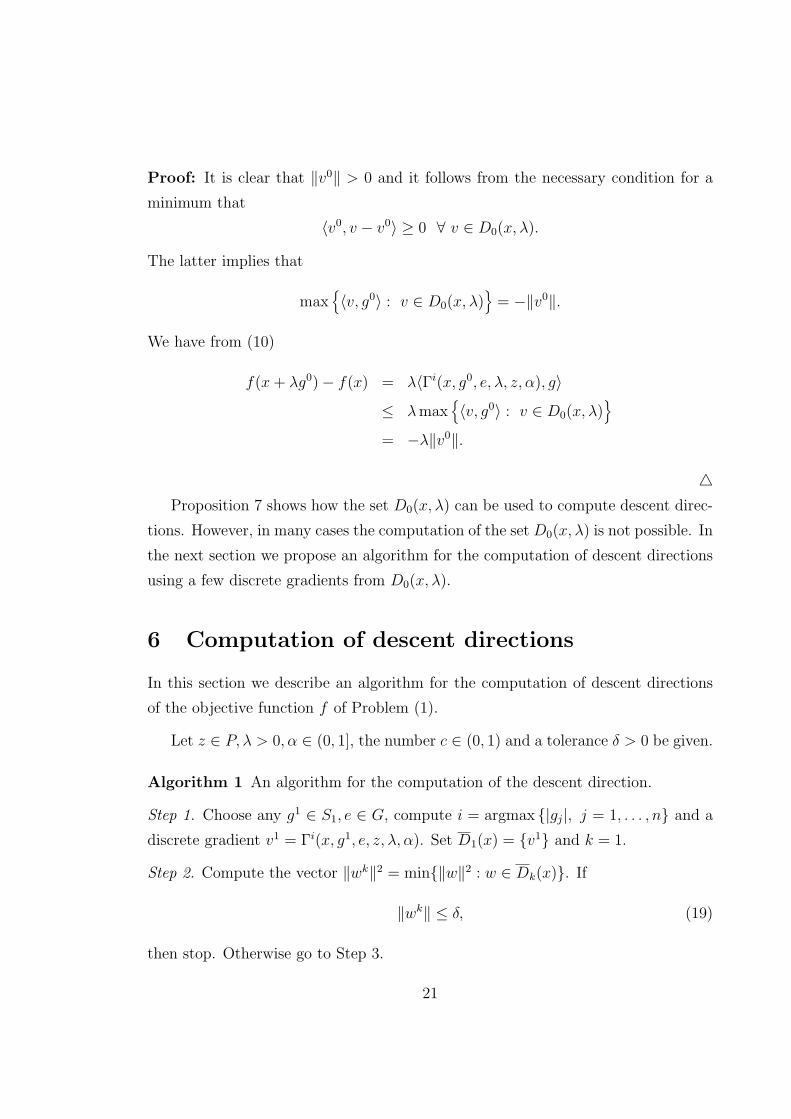
4Proposition 7 shows how the set D0(x, λ) can be used to compute descent direc-

tions. However, in many cases the computation of the set D0(x, λ) is not possible. In

the next section we propose an algorithm for the computation of descent directions

using a few discrete gradients from D0(x, λ).

6 Computation of descent directions

In this section we describe an algorithm for the computation of descent directions

of the objective function f of Problem (1).

Let z ∈ P, λ > 0, α ∈ (0, 1], the number c ∈ (0, 1) and a tolerance δ > 0 be given.

Algorithm 1 An algorithm for the computation of the descent direction.

Step 1. Choose any g1 ∈ S1, e ∈ G, compute i = argmax {|gj|, j = 1, . . . , n} and a

discrete gradient v1 = Γi(x, g1, e, z, λ, α). Set D1(x) = {v1} and k = 1.

Step 2. Compute the vector ‖wk‖2 = min{‖w‖2 : w ∈ Dk(x)}. If

‖wk‖ ≤ δ, (19)

then stop. Otherwise go to Step 3.

21

Step 3. Compute the search direction by gk+1 = −‖wk‖−1wk.

Step 4. If

f(x + λgk+1)− f(x) ≤ −cλ‖wk‖, (20)

then stop. Otherwise go to Step 5.

Step 5. Compute i = argmax {|gk+1j | : j = 1, . . . , n} and a discrete gradient

vk+1 = Γi(x, gk+1, e, z, λ, α),

construct the set Dk+1(x) = co {Dk(x)⋃{vk+1}}, set k = k + 1 and go to Step 2.

We give some explanations to Algorithm 1. In Step 1 we compute the discrete

gradient with respect to an initial direction g1 ∈ IRn. The distance between the

convex hull Dk(x) of all computed discrete gradients and the origin is computed

in Step 2. This problem can be solved using the algorithm from [22] (for more

recent approaches to this problem, see also [23, 24]). If this distance is less than

the tolerance δ > 0 then we accept the point x as an approximate stationary point

(Step 2), otherwise we compute another search direction in Step 3. In Step 4 we

check whether this direction is a descent direction. If it is we stop and the descent

direction has been computed, otherwise we compute another discrete gradient with

respect to this direction in Step 5 and update the set Dk(x). At each iteration k we

improve the approximation of the subdifferential of the function f .

In the next proposition we prove that Algorithm 1 terminates after a finite num-

ber of iterations.

Proposition 8 Let f be a locally Lipschitz function defined on IRn. Then for δ ∈(0, C) either the condition (19) or the condition (20) satisfy after m computations

of the discrete gradients where

m ≤ 2(log2(δ/C)/ log2 r + 1), r = 1− [(1− c)(2C)−1δ]2,

C = C(n)L and C(n) is a constant from Proposition 4.

22

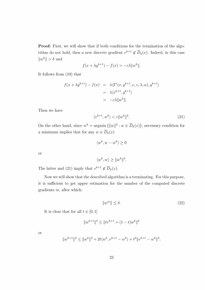
Proof: First, we will show that if both conditions for the termination of the algo-

rithm do not hold, then a new discrete gradient vk+1 6∈ Dk(x). Indeed, in this case

‖wk‖ > δ and

f(x + λgk+1)− f(x) > −cλ‖wk‖.It follows from (10) that

f(x + λgk+1)− f(x) = λ〈Γi(x, gk+1, e, z, λ, α), gk+1〉= λ〈vk+1, gk+1〉> −cλ‖wk‖.

Then we have

〈vk+1, wk〉 < c‖wk‖2. (21)

On the other hand, since wk = argmin {‖w‖2 : w ∈ Dk(x)}, necessary condition for

a minimum implies that for any w ∈ Dk(x)

〈wk, w − wk〉 ≥ 0

or

〈wk, w〉 ≥ ‖wk‖2.

The latter and (21) imply that vk+1 6∈ Dk(x).

Now we will show that the described algorithm is a terminating. For this purpose,

it is sufficient to get upper estimation for the number of the computed discrete

gradients m, after which:

‖wm‖ ≤ δ. (22)

It is clear that for all t ∈ [0, 1]

‖wk+1‖2 ≤ ‖tvk+1 + (1− t)wk‖2

or

‖wk+1‖2 ≤ ‖wk‖2 + 2t〈wk, vk+1 − wk〉+ t2‖vk+1 − wk‖2.

23

It follows from Proposition 4 that

‖vk+1 − wk‖ ≤ 2C.

Hence taking into account the inequality (21), we have

‖wk+1‖2 < ‖wk‖2 − 2t(1− c)‖wk‖2 + 4t2C2.

For t = (1− c)(2C)−2‖wk‖2 ∈ (0, 1) we get

‖wk+1‖2 <{1− [(1− c)(2C)−1‖wk‖]2

}‖wk‖2. (23)

Let δ ∈ (0, C). It follows from (23) and the condition ‖wk‖ > δ, k = 1, . . . ,m − 1

that

‖wk+1‖2 <{1− [(1− c)(2C)−1δ]2

}‖wk‖2.

We denote by r = 1− [(1− c)(2C)−1δ]2. It is clear that r ∈ (0, 1). Then we have

‖wm‖2 < r‖wm−1‖2 < . . . < rm−1‖w1‖2 < rm−1C2.

If rm−1C2 ≤ δ2, then the inequality (22) is also true and therefore,

m ≤ 2(log2(δ/C)/ log2 r + 1).

4

Remark 7 Proposition 4 and the equality (10) are true for any λ > 0 and for any

locally Lipschitz continuous functions. This means that Algorithm 1 can compute

descent directions for any λ > 0 and for any locally Lipschitz continuous functions

in a finite number of iterations. Sufficiently small values of λ give an approximation

to the subdifferential and in this case Algorithm 1 computes local descent directions.

For such directions f(x + αg) < f(x) for all α ∈ (0, λ]. Larger values of λ do not

give an approximation to the subdifferential and in this case for descent directions

computed by Algorithm 1 f(x + λg) < f(x), however for sufficiently small α > 0

one can expect that f(x + αg) ≥ f(x). Such directions exist at local minimizers

which are not global minimizers. We call them global descent directions.

24

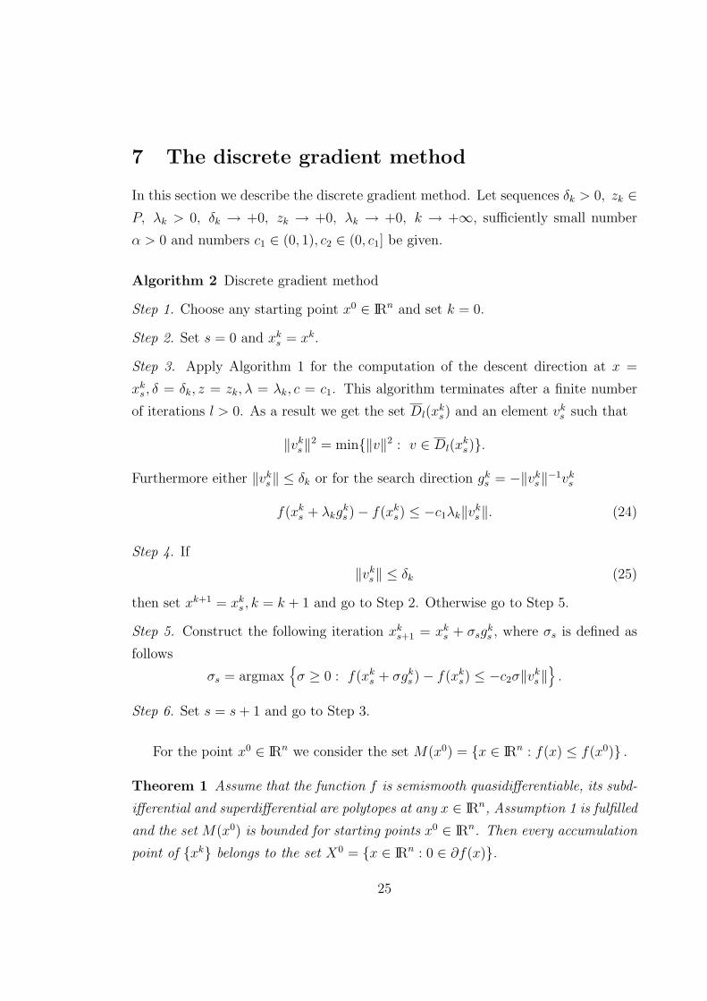
7 The discrete gradient method

In this section we describe the discrete gradient method. Let sequences δk > 0, zk ∈P, λk > 0, δk → +0, zk → +0, λk → +0, k → +∞, sufficiently small number

α > 0 and numbers c1 ∈ (0, 1), c2 ∈ (0, c1] be given.

Algorithm 2 Discrete gradient method

Step 1. Choose any starting point x0 ∈ IRn and set k = 0.

Step 2. Set s = 0 and xks = xk.

Step 3. Apply Algorithm 1 for the computation of the descent direction at x =

xks , δ = δk, z = zk, λ = λk, c = c1. This algorithm terminates after a finite number

of iterations l > 0. As a result we get the set Dl(xks) and an element vk

s such that

‖vks‖2 = min{‖v‖2 : v ∈ Dl(x

ks)}.

Furthermore either ‖vks‖ ≤ δk or for the search direction gk

s = −‖vks‖−1vk

s

f(xks + λkg

ks )− f(xk

s) ≤ −c1λk‖vks‖. (24)

Step 4. If

‖vks‖ ≤ δk (25)

then set xk+1 = xks , k = k + 1 and go to Step 2. Otherwise go to Step 5.

Step 5. Construct the following iteration xks+1 = xk

s + σsgks , where σs is defined as

follows

σs = argmax{σ ≥ 0 : f(xk

s + σgks )− f(xk

s) ≤ −c2σ‖vks‖

}.

Step 6. Set s = s + 1 and go to Step 3.

For the point x0 ∈ IRn we consider the set M(x0) = {x ∈ IRn : f(x) ≤ f(x0)} .

Theorem 1 Assume that the function f is semismooth quasidifferentiable, its subd-

ifferential and superdifferential are polytopes at any x ∈ IRn, Assumption 1 is fulfilled

and the set M(x0) is bounded for starting points x0 ∈ IRn. Then every accumulation

point of {xk} belongs to the set X0 = {x ∈ IRn : 0 ∈ ∂f(x)}.

25

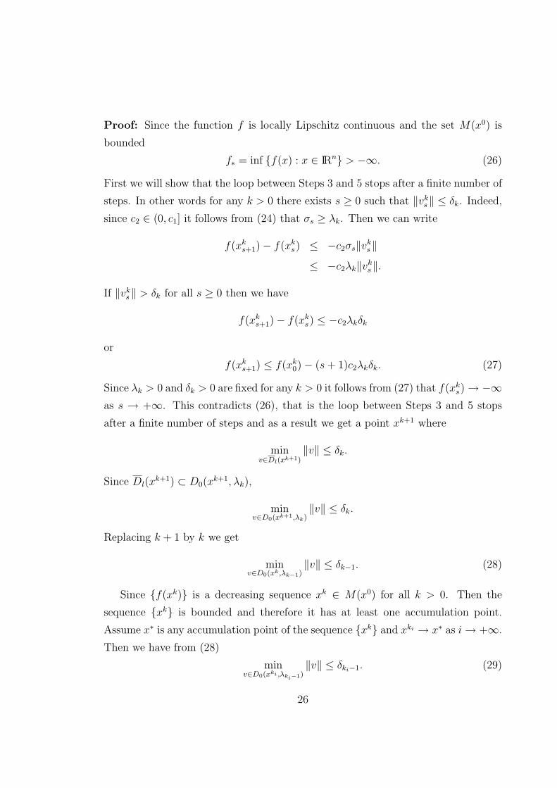
Proof: Since the function f is locally Lipschitz continuous and the set M(x0) is

bounded

f∗ = inf {f(x) : x ∈ IRn} > −∞. (26)

First we will show that the loop between Steps 3 and 5 stops after a finite number of

steps. In other words for any k > 0 there exists s ≥ 0 such that ‖vks‖ ≤ δk. Indeed,

since c2 ∈ (0, c1] it follows from (24) that σs ≥ λk. Then we can write

f(xks+1)− f(xk

s) ≤ −c2σs‖vks‖

≤ −c2λk‖vks‖.

If ‖vks‖ > δk for all s ≥ 0 then we have

f(xks+1)− f(xk

s) ≤ −c2λkδk

or

f(xks+1) ≤ f(xk

0)− (s + 1)c2λkδk. (27)

Since λk > 0 and δk > 0 are fixed for any k > 0 it follows from (27) that f(xks) → −∞

as s → +∞. This contradicts (26), that is the loop between Steps 3 and 5 stops

after a finite number of steps and as a result we get a point xk+1 where

minv∈Dl(xk+1)

‖v‖ ≤ δk.

Since Dl(xk+1) ⊂ D0(x

k+1, λk),

minv∈D0(xk+1,λk)

‖v‖ ≤ δk.

Replacing k + 1 by k we get

minv∈D0(xk,λk−1)

‖v‖ ≤ δk−1. (28)

Since {f(xk)} is a decreasing sequence xk ∈ M(x0) for all k > 0. Then the

sequence {xk} is bounded and therefore it has at least one accumulation point.

Assume x∗ is any accumulation point of the sequence {xk} and xki → x∗ as i → +∞.

Then we have from (28)

minv∈D0(xki ,λki−1)

‖v‖ ≤ δki−1. (29)

26

According to Assumption 1 at the point x∗ for any ε > 0 there exist β > 0 and

λ0 > 0 such that

D0(y, λ) ⊂ ∂f(x∗ + Sε) + Sε (30)

for all y ∈ Sβ(x∗) and λ ∈ (0, λ0). Since the sequence {xki} converges to x∗ for

β > 0 there exists i0 > 0 such that xki ∈ Sβ(x∗) for all i ≥ i0. On the other hand

since δk, λk → 0 as k → +∞ there exists k0 > 0 such that δk < ε and λk < λ0 for

all k > k0. Then there exists i1 ≥ i0 such that ki ≥ k0 + 1 for all i ≥ i1. Thus it

follows from (29) and (30) that

minv∈∂f(x∗+Sε)

‖v‖ ≤ 2ε

Since ε > 0 is arbitrary and the mapping ∂f(x) is upper semicontinuous 0 ∈ ∂f(x∗).

4Remark 8 Since Algorithm 1 can compute descent directions for any values of

λ > 0 we take λ0 ∈ (0, 1), some β ∈ (0, 1) and update λk, k ≥ 1 as follows:

λk = βkλ0, k ≥ 1.

Thus in the discrete gradient method we use approximations to subgradients only at

the final stage of the method which guarantees convergence. In most of iterations we

do not use explicit approximations of subgradients. Therefore it is a derivative-free

method.

Remark 9 One can see some similarity between the discrete gradient and bundle-

type methods. More specifically, the method presented in this paper can be con-

sidered as a derivative-free version of the bundle method introduced in [25]. The

main difference is that in the proposed method discrete gradients are used instead

of subgradients at some points from neighborhood of a current point. The discrete

gradients need not to be approximations to subgradients at all iterations.

Remark 10 It follows from (24) and c2 ≤ c1 that always σs ≥ λk and therefore

λk > 0 is a lower bound for σs. This leads to the following rule for the computation

of σs. We define a sequence:

θm = mλk, m ≥ 1

and σs is defined as the largest θm satisfying the inequality in Step 5.

27

8 Numerical experiments

The efficiency of the proposed algorithm was verified by applying it to some un-

constrained nonsmooth optimization problems. In numerical experiments we use 20

unconstrained test problems from [26]: Problems 2.1-7 (P1-P7), 2.9-12 (P9-P12),

2.14-16 (P14-P16), 2.18-21 (P18-P21), 2.23-24 (P23, P24).

Objective functions in these problems are discrete maximum functions and they

are regular. Objective functions in Problems 2.1, 2.5, 2.23 are convex and they are

nonconvex in all other problems. This means that most of problems are problems

of global optimization and the same algorithm may find different solutions starting

from different initial points and/or different algorithms may find different solutions

starting from the same initial point. The brief description of these problems is given

in Table 1 where the following notation is used:

• n - number of variables;

• nm - number of functions under maximum;

• fopt - optimum value (as reported in [26]).

For the comparison we use DNLP model of CONOPT solver from The General

Algebraic Modeling System (GAMS) and CONDOR solver. DNLP is nonsmooth

optimization solver and it is based on smoothing techniques. More details on DNLP

can be found in [27]. CONDOR is a derivative free solver based on quadratic inter-

polation and trust region approach (see, [28] for more details).

Numerical experiments were carried out on PC Pentium 4 with CPU 1.6 MHz.

We used 20 random initial points for each problem and initial points are the same

for all three algorithms.

The results of numerical experiments are presented in Table 2. We use the

following notation:

• fbest and fav - the best and average objective function values over 20 runs,

respectively;

28

Table 1: The brief description of test problems

Prob. n nm fopt Prob. n nm fopt

P1 2 3 1.95222 P12 4 21 0.00202

P2 2 3 0 P14 5 21 0.00012

P3 2 2 0 P15 5 30 0.02234

P4 3 6 3.59972 P16 6 51 0.03490

P5 4 4 -44 P18 9 41 0.00618

P6 4 4 -44 P19 7 5 680.63006

P7 3 21 0.00420 P20 10 9 24.30621

P9 4 11 0.00808 P21 20 18 133.72828

P10 4 20 115.70644 P23 11 10 261.08258

P11 4 21 0.00264 P24 20 31 0.00000

• nfc - the average number of the objective function evaluations (for the discrete

gradient method (DGM) and CONDOR);

• iter - the average number of iterations (for DNLP);

• DN stands for DNLP and CR for CONDOR;

• F means that an algorithm failed for all initial points.

One can draw the following conclusions from Table 2:

1. The discrete gradient method finds the best solutions for all problems whereas

the CONDOR solver could find the best solutions only for Problems 1.1-3 and

the DNLP solver only for Problems 1.1, 1.4.

2. Average results over 20 runs by the discrete gradient method are better than

those by the DNLP and CONDOR solvers, except Problems 2.2, 2.3, 2.6, 2.7

and 2.24 where the CONDOR solver produces better results.

3. For three convex problems 2.1, 2.5 and 2.23 the discrete gradient method

always finds the same solutions, that is the best and average results by this

29

method are the same with respect to some tolerance. However this is not the

case for the DNLP and CONDOR solvers.

4. For many test problems results by the DNLP solver are significantly worse

than those by the CONDOR solver and the discrete gradient method. In these

problems the values of objective functions or their gradients is too large and

the DNLP solver fails to solve such problems. Results for Problems 2.6 and

2.23 demonstrate it. However the CONDOR solver and the discrete gradients

method are quite efficient to solve such problems.

5. As it was mentioned above the most of the test problems are global optimiza-

tion problems. Results presented clearly demonstrate that the derivative-free

methods are better than Newton-like methods to solve global optimization

problems. Overall the discrete gradient method outperforms other two meth-

ods.

6. One can see from Table 2 that the number of function calls by the CONDOR

solver is significantly less than those by the discrete gradient method. How-

ever, there is no any significant difference in the CPU time used by different

algorithms.

Since the most of test problems are nonconvex we suggest the following scheme

to compare the performance of algorithms for each run. Let f be the best value

obtained by all algorithm starting from the same initial point. Let f 1 be the value

of the objective function at the final point obtained by an algorithm. If

f 1 − f ≤ ε(|f |+ 1)

then we say that this algorithm finds the best result with respect to the tolerance

ε > 0. Tables 3 and 4 present pairwise comparison and the comparison of three

algorithms, respectively. The numbers in these tables show how many times an

algorithm could find the best solution with respect to the tolerance ε = 10−4. Results

presented in Table 3 demonstrate that the CONDOR solver outperforms the DNLP

solver in 90 % of runs, the discrete gradient method outperforms the DNLP solver

30

in more than 95 % of runs and finally the discrete gradient method outperforms the

CONDOR solver in almost 80 % of runs.

Results presented in Table 4 show that the discrete gradient method outperforms

other two solvers in all problems except Problems 2.3 and 2.7 where the CONDOR

solver outperforms others.

Overall results presented in this paper demonstrate that the discrete gradient

method is more efficient than the DNLP and CONDOR solvers for solving nons-

mooth nonconvex optimization problems.

9 Conclusions

In this paper we have proposed a derivative free algorithm, the discrete gradient

method for solving unconstrained nonsmooth optimization problems. This algo-

rithm can be applied to a broad class of nonsmooth optimization problems including

problems with non-regular objective functions.

We have tested the new algorithm on some nonsmooth optimization problems. In

the most of these problems the objective functions are regular nonconvex functions.

For comparison we used one nonsmooth optimization algorithm: DNLP solver from

GAMS which is based on the smoothing of the objective function and one derivative

free CONDOR solver which is based on the quadratic approximation of the objective

function. Preliminary results of our numerical experiments show that the discrete

gradient method outperforms other two algorithms for the most of test problems

considered in this paper. Our results also demonstrate that derivative-free methods

are better than Newton-like methods for solving global optimization problems. We

can conclude that the discrete gradient method is a good alternative to existing

derivative-free nonsmooth optimization algorithms.

Acknowledgements

The authors are grateful to the anonymous referee for comments improving the qual-

ity of the paper. The research by the first author was supported by the Australian

Research Council.

31

References

[1] HIRIART-URRUTY, J.B. and LEMARCHAL, C., Convex Analysis and Min-

imization Algorithms, Springer Verlag, Heidelberg, Vol. 1 and 2, 1993.

[2] KIWIEL, K.C., Methods of Descent for Nondifferentiable Optimization, Lec-

ture Notes in Mathematics, Springer-Verlag, Berlin, Vol. 1133, 1985.

[3] KIWIEL, K.C., Proximal control in bundle methods for convex nondifferen-

tiable minimization, Mathematical Programming, Vol. 29, pp. 105-122, 1990.

[4] LEMARCHAL, C., An extension of Davidon methods to nondifferentiable

problems , Nondifferentiable Optimization, Balinski, M.L. and Wolfe, P. (eds.),

Mathematical Programming Study, Vol. 3, pp. 95-109, North-Holland, Ams-

terdam, 1975.

[5] LEMARCHAL, C., and ZOWE, J., A condensed introduction to bundle meth-

ods in nonsmooth optimization, In: Algorithms for Continuous Optimization,

Spedicato, E. (ed.,), pp. 357 - 482, Kluwer Academic Publishers, 1994.

[6] MIFFLIN, R., An algorithm for constrained optimization with semismooth

functions , Math. Oper. Res., Vol. 2, pp. 191-207, 1977.

[7] ZOWE, J., Nondifferentiable optimization: A motivation and a short intro-

duction into the subgradient and the bundle concept , In: NATO SAI Series,

Vol. 15, Computational Mathematical Programming, Schittkowski, K., (ed.),

pp. 323-356, Springer-Verlag, New York, 1985.

[8] POLAK, E. and ROYSET, J.O., Algorithms for finite ans semi-infinite min-

max-min problems using adaptive smoothing techniques , Journal of Optimiza-

tion Theory and Applications, Vol. 119, pp. 421-457, 2003.

[9] BURKE, J.V., LEWEIS, A.S. and OVERTON, M.L., Approximating subdiffer-

entials by random sampling of gradients , Mathematics of Operations Research,

Vol. 27, pp. 567-584, 2002.

32

[10] AUDET, C. and DENNIS, J.E., Jr., Analysis of generalized pattern searches ,

SIAM Journal on Optimization, Vol. 13, pp. 889-903, 2003.

[11] TORZCON, V., On the convergence of pattern search algorithms , SIAM Jour-

nal on Optimization, Vol. 7, pp. 1-25, 1997.

[12] CLARKE, F.H., Optimization and Nonsmooth Analysis, New York: John Wi-

ley, 1983.

[13] MIFFLIN, R., Semismooth and semiconvex functions in constrained optimiza-

tion, SIAM J. Control and Optimization, Vol. 15, pp. 959-972, 1977.

[14] DEMYANOV, V.F. and RUBINOV, A.M., Constructive Nonsmooth Analysis,

Peter Lang, Frankfurt am Main, 1995.

[15] BAGIROV, A.M., RUNINOV, A.M. and YEARWOOD, J., A global optimi-

sation approach to classification, Optimization and Engineering, Vol. 3, pp.

129-155, 2002.

[16] BAGIROV, A.M., RUBINOV, A.M., SOUKHOROUKOVA, A.V., and YEAR-

WOOD, J., Supervised and unsupervised data classification via nonsmooth and

global optimisation, TOP: Spanish Operations Research Journal, Vol. 11, pp.

1-93, 2003.

[17] BAGIROV, A.M. and UGON, J., An algorithm for minimizing clustering func-

tions , Optimization, Vol. 54, pp. 351-368, 2005.

[18] BAGIROV, A.M. and YEARWOOD, J., A new nonsmooth optimisation algo-

rithm for minimum sum-of-squares clustering problems , European Journal of

Operational Research, Vol. 170, pp. 578-596, 2006.

[19] BAGIROV, A.M. and GASANOV, A.A., A method of approximating a quasid-

ifferential , Journal of Computational Mathematics and Mathematical Physics,

Vol. 35, pp. 403-409, 1995.

[20] BAGIROV, A.M., Minimization methods for one class of nonsmooth func-

tions and calculation of semi-equilibrium prices , In: A. Eberhard et al. (eds.),

33

Progress in Optimization: Contribution from Australasia, pp. 147-175, Kluwer

Academic Publishers, 1999.

[21] BAGIROV, A.M. , Continuous subdifferential approximations and their appli-

cations , Journal of Mathematical Sciences, Vol. 115, pp. 2567-2609, 2003.

[22] WOLFE, P.H., Finding the nearest point in a polytope, Mathematical Pro-

gramming, Vol. 11, pp. 128-149, 1976.

[23] FRANGONI, A., Solving semidefinite quadratic problems within nonsmooth

optimization algorithms , Comput. Oper. Res. Vol. 23, pp. 1099-1118, 1996.

[24] KIWIEL, K.C., A dual method for certainpositive semidefinite quadratic pro-

gramming problems , SIAM J. Sci. Statist. Comput. Vol. 10, pp. 175-186, 1989.

[25] WOLFE, P.H., A method of conjugate subgradients of minimizing nondiffer-

entiable convex functions , Mathematical Programming Study, Vol. 3, pp. 145-

173, 1975.

[26] LUKSAN, L. and VLECK, J., Test Problems for Nonsmooth Unconstrained

and Linearly Constrained Optimization, Technical Report No. 78, Institute of

Computer Science, Academy of Sciences of the Czech Republic, 2000.

[27] GAMS: The Solver Manuals , GAMS Development Corporation, Washington,

D.C., 2004.

[28] BERGEN, F. V., CONDOR: a constrained, non-linear, derivative-free parallel

optimizer for continuous, high computing load, noisy objective functions , PhD

thesis, Universite Libre de Bruxelles, Belgium, 2004.

34

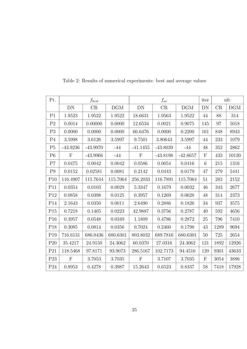
Table 2: Results of numerical experiments: best and average values

Pr. fbest fav iter nfc

DN CR DGM DN CR DGM DN CR DGM

P1 1.9523 1.9522 1.9522 18.6631 1.9563 1.9522 44 88 314

P2 0.0014 0.00000 0.0000 12.6534 0.0021 0.9075 145 97 5018

P3 0.0000 0.0000 0.0000 66.6476 0.0000 0.2200 161 848 8943

P4 3.5998 3.6126 3.5997 9.7501 3.80643 3.5997 44 233 1079

P5 -43.9236 -43.9970 -44 -41.1455 -43.8039 -44 48 352 2862

P6 F -43.9966 -44 F -43.8198 -42.8657 F 433 10120

P7 0.0475 0.0042 0.0042 0.0586 0.0054 0.0416 6 215 1316

P9 0.0152 0.02581 0.0081 0.2142 0.0443 0.0179 47 279 5441

P10 116.4907 115.7644 115.7064 256.2033 116.7891 115.7064 51 283 2152

P11 0.0354 0.0103 0.0029 5.3347 0.1679 0.0032 46 343 2677

P12 0.0858 0.0398 0.0125 0.3957 0.1269 0.0628 48 314 2373

P14 2.1643 0.0350 0.0011 2.6490 0.2886 0.1826 34 937 3575

P15 0.7218 0.1405 0.0223 42.9887 0.3756 0.2787 40 592 4656

P16 0.3957 0.0548 0.0349 1.1809 0.4786 0.2872 25 796 7410

P18 0.3085 0.0814 0.0356 0.7024 0.2460 0.1798 43 1289 9694

P19 716.6131 686.0436 680.6301 803.8032 689.7816 680.6301 50 725 2654

P20 35.4217 24.9150 24.3062 60.0370 27.0316 24.3062 121 1892 12926

P21 118.5468 97.8171 93.9073 286.5167 102.7173 94.4516 120 9301 43633

P23 F 3.7053 3.7035 F 3.7107 3.7035 F 3054 3886

P24 0.8953 0.4278 0.3987 15.2643 0.6523 0.8337 58 7418 17928

35

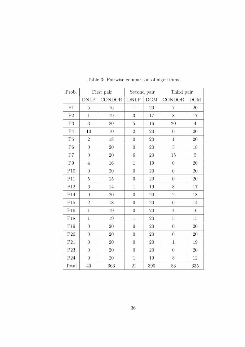
Table 3: Pairwise comparison of algorithms

Prob. First pair Second pair Third pair

DNLP CONDOR DNLP DGM CONDOR DGM

P1 5 16 1 20 7 20

P2 1 19 3 17 8 17

P3 3 20 5 16 20 4

P4 10 10 2 20 0 20

P5 2 18 0 20 1 20

P6 0 20 0 20 3 18

P7 0 20 6 20 15 5

P9 4 16 1 19 0 20

P10 0 20 0 20 0 20

P11 5 15 0 20 0 20

P12 6 14 1 19 3 17

P14 0 20 0 20 2 18

P15 2 18 0 20 6 14

P16 1 19 0 20 4 16

P18 1 19 1 20 5 15

P19 0 20 0 20 0 20

P20 0 20 0 20 0 20

P21 0 20 0 20 1 19

P23 0 20 0 20 0 20

P24 0 20 1 19 8 12

Total 40 363 21 390 83 335

36

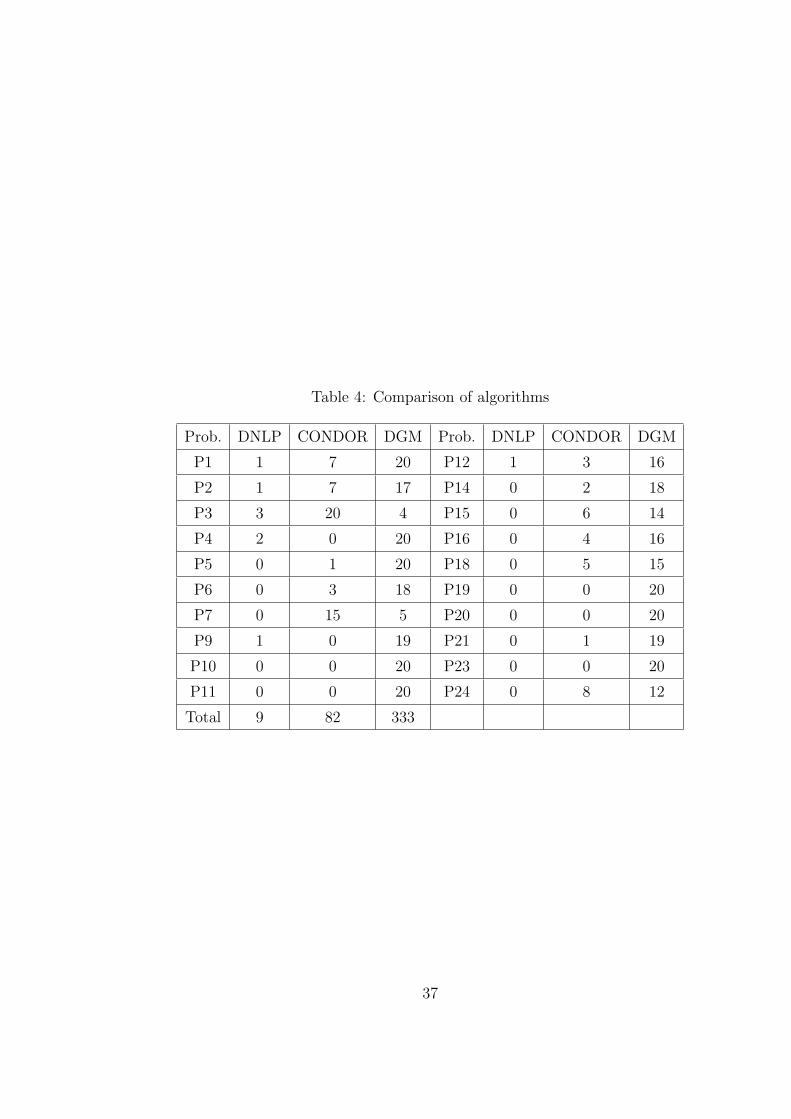
Table 4: Comparison of algorithms

Prob. DNLP CONDOR DGM Prob. DNLP CONDOR DGM

P1 1 7 20 P12 1 3 16

P2 1 7 17 P14 0 2 18

P3 3 20 4 P15 0 6 14

P4 2 0 20 P16 0 4 16

P5 0 1 20 P18 0 5 15

P6 0 3 18 P19 0 0 20

P7 0 15 5 P20 0 0 20

P9 1 0 19 P21 0 1 19

P10 0 0 20 P23 0 0 20

P11 0 0 20 P24 0 8 12

Total 9 82 333

37